Bridging Model Reference Adaptive
Control and Data Informativity

Abstract

The goal of model reference adaptive control (MRAC) is to ensure that the trajectories of an unknown dynamical system track those of a given reference model. This is done by means of a feedback controller that adaptively changes its gains using data collected online from the closed-loop system. One of the approaches to solve the MRAC problem is to impose conditions on the data that guarantee convergence of the gains to a solution of the so-called matching equations. In the literature, various extensions of the concept of persistent excitation have been proposed in an effort to weaken the conditions on the data required for this convergence. Despite these efforts, it is not well-understood what are the weakest possible data requirements ensuring convergence of MRAC. In this paper, we propose a new framework to study the MRAC problem, using the concept of data informativity. Our main contribution is to provide necessary and sufficient conditions for the convergence of the adaptive gains to a solution of the matching equations. These necessary and sufficient conditions can be readily checked online as new data are generated by the closed-loop system. Our results reveal that existing excitation conditions impose stronger requirements on the collected data than required. Notably, the necessary and sufficient conditions provided in this paper are weaker than those for unique system identification.

Multi-variable MRAC, persistence of excitation, parameter convergence, data informativity.

1 Introduction

Adaptive control has a rich history, which can be traced back to pioneering work from the 1950s [1]. Adaptive control aims at dealing with the inevitable uncertainty in control systems by means of adjustable-gain controllers, that are adapted online using the data generated by the closed-loop system. Among the various adaptive control strategies developed over the years, a common approach is model reference adaptive control (MRAC), where the control gains are adjusted so that the closed-loop system tracks a predefined reference model [2].

Meanwhile, offline data-driven control approaches also have a rich history: here, the system to be controlled is uncertain as in adaptive control, but the data are collected offline [3, 4]. In this setting, the controller is constructed in one shot using a batch of data. Among the various offline data-driven control strategies, the data informativity approach has recently emerged [5]. Data informativity provides necessary and sufficient conditions under which the data contain sufficient information for control design. In what follows, we provide an overview of representative MRAC approaches and data informativity approaches, so as to clarify the gaps in the respective fields and how these gaps are closed in this work.

1.1 State of the art on data requirements in MRAC

Despite decades of history, MRAC still remains a prominent research area, with advances continually emerging, such as switched MRAC [6, 7, 8], robust MRAC [9, 10], distributed MRAC [11, 12], partial-state feedback MRAC [13], and learning-based MRAC [14, 15], just to mention a few. The key concept common to all MRAC approaches are the matching equations: control gains must exist so that the closed-loop system matches the dynamics of the reference model. Assuming the matching equations have a solution, the question is whether the online adjustment mechanism converges to such a solution. Here and in the following, we say that an adjustment mechanism ‘solves’ the MRAC problem if it guarantees the convergence of the adaptive gains to a solution of the matching equations.

It is well known that classical MRAC approaches (direct or indirect [16, 17]) need to impose requirements on the closed-loop data to guarantee convergence to a solution of the matching equations [18]. The most traditional requirement goes under the name of persistence of excitation (PE), which requires the excitation provided by the input data to never vanish [19]. A very productive line of research has been devoted to relaxing the requirements imposed on data that allow to solve the MRAC problem. Representative methods are composite/combined MRAC [20], concurrent learning MRAC [21], and works where PE has been relaxed to rank excitation [22], finite excitation [23, 24] and initial excitation [25, 26]. While all these relaxed excitation conditions are sufficient to solve the MRAC problem, a natural question is whether they are also necessary. Our work will show that the relaxed excitation conditions in the literature are, in general, not necessary to solve the MRAC problem.

It is worth mentioning that although most of the methods above address multi-variable MRAC problems (where the number of inputs and reference signals is larger than one [27]), such a multi-variable setting requires additional assumptions on the system to arrive at a solution to the problem. It is common in multi-variable MRAC to require a known system’s input matrix [27, 20, 21, 22, 23, 24] or other structural assumptions [28, 29, 25, 30] to handle the uncertainty. Our work will remove such restrictions, requiring no prior knowledge on the input matrix and no other structural assumptions on the unknown system apart from controllability. Moreover, we are able to solve the MRAC problem even when the matching equations have a possibly infinite number of solutions, in contrast with existing multi-variable MRAC approaches where the structural assumptions are such that only one solution of the matching equations exists.

1.2 State of the art on adaptation in data informativity

In the literature on offline data-driven control, a key role is played by Willems et al.’s fundamental lemma [31]. This result provides a data-dependent representation of the system based on persistently exciting data [4, 32, 33, 34]. Similar to the quest for relaxed PE requirements in adaptive control, research efforts have been made to relax the requirement for persistently exciting data. An answer in this direction was provided by the data informativity framework [5], demonstrating that PE is not necessary in several data-driven analysis and control problems; also see [35] for more details. By adopting the data informativity perspective, [36] studied the requirements that data must have in order to solve an offline model reference control: there, it was shown that persistently exciting data are also not necessary for solving such problem.

However, offline data-driven control is intrinsically different from MRAC, because the data are not generated online by the time-varying closed-loop system obtained from interconnecting the dynamical system and the adaptive feedback law. Indeed, in existing work on the data informativity framework, controllers are constructed offline in one shot, using a batch of data. Online experiment design procedures have been studied in [37]: however, such procedures only aim at generating a batch of informative data and do not incorporate a control objective, as is customary in adaptive control. This motivates us to further investigate the relation between MRAC and data informativity. In particular, a key question is: can data informativity be turned from an offline framework to an online one, where data are generated in real-time by the closed-loop system as the controller is adjusted online? In this work, we develop a novel MRAC approach based on the concept of data informativity, thus bridging these two realms. Because data informativity has been shown to give necessary and sufficient conditions for several data-driven control problems, a crucial question is: can necessary and sufficient conditions be obtained for the convergence of MRAC? This work gives a positive answer, thus providing a non-conservative condition on data that allows to solve the MRAC problem.

1.3 Contributions

This paper studies multi-variable MRAC using the framework of data informativity. The main contributions are as follows:

• We investigate the connection between data informativity for model reference control [36] and data informativity for system identification (cf. Proposition 4.2 & Theorem 4.4). Specifically, we show that data informativity for system identification is sufficient but not necessary for data informativity for model reference control. It becomes necessary only in special cases. This sets the stage for studying MRAC through the lens of data informativity.

• We propose an MRAC approach that only exploits data informativity for model reference control, without relying on data informativity for system identification or persistence of excitation conditions. The framework relies on data informativity as in work by the authors on offline model reference control [36]. However, we develop new conditions for data informativity for model reference control that can be checked online, as data are generated at every time step by the closed-loop system. This provides an online method for collecting informative data (Lemma 5.7), which is then utilized to design a controller along with an adaptive law. The online collection of informative data marks a key difference with different types of online approaches [38, 39, 40] where the conditions on data are assumed a priori rather than imposed by suitable design of the inputs. We also prove that, with the proposed online method, the controller gains will converge to a solution of the matching equations (Theorem 5.11), and the tracking error is bounded and will converge to zero (Theorem 5.16).

• The proposed conditions for convergence to a solution of the matching equations are necessary and sufficient, and thus do not introduce any conservatism. Furthermore, our MRAC method operates on general multi-variable input-state systems without structural assumptions on the unknown system matrices. Even in scenarios where the ideal controller is not unique, our framework guarantees that the controller parameters will converge to a solution of the matching equations.

1.4 Outline

The remainder of this paper is structured as follows. In Section II, notation and preliminary results about Willems et al.’s fundamental lemma are provided. Section III presents the mathematical formulation of MRAC. In Section IV, key results on data informativity for system identification and data informativity for model reference control are recalled and compared. The proposed framework for online MRAC is presented in Section V, including necessary and sufficient conditions for the convergence to a solution of the matching equations. This section also discusses how the proposed solution relates to the requirements imposed on data in state-of-the-art MRAC methods. In Section VI, a numerical example of a highly maneuverable aircraft is provided. Concluding remarks are given in Section VII.

2 Preliminaries

2.1 Notation

We denote the set of positive integers by $\mathbb{N}$, the set of non-negative integers by $\mathbb{Z}_{+}$, and the set of non-negative real numbers by $\mathbb{R}_{+}$. The Euclidean norm of a vector $v\in\mathbb{R}^{n}$ is denoted by $|v|$. The Frobenius norm and induced $2$-norm of a matrix $A\in\mathbb{R}^{n\times m}$ are denoted by $\|A\|_{F}$ and $\|A\|_{2}$, respectively. The identity matrix of appropriate size is denoted by $I$. A square matrix is called Schur if all its eigenvalues have modulus strictly less than 1, and is Hurwitz if all its eigenvalues have negative real part. A symmetric matrix $A=A^{\top}\in\mathbb{R}^{n\times n}$ is said to be positive definite (denoted by $A>0$) if $v^{\top}Av>0$ for all nonzero $v\in\mathbb{R}^{n}$. Moreover, $A$ is called positive semidefinite if $v^{\top}Av\geq 0$ for all $v\in\mathbb{R}^{n}$. This is denoted by $A\geq 0$. For two symmetric $n\times n$ matrices $A$ and $B$, we use the notation $A\geq B$, meaning that $A-B\geq 0$. We denote by $\ell_{\infty}^{n,m}$ the space of all sequences $\{S(t)\}_{t=0}^{\infty}$ for which $S(t)\in\mathbb{R}^{n\times m}$ and

$$||S||_{\infty}:=\sup_{t\in\mathbb{Z}_{+}}||S(t)||_{2}<\infty.$$

In addition, we use the shorthand notation $\ell_{\infty}^{n}:=\ell_{\infty}^{n,1}$.

2.2 Behaviors and Willems et al.’s fundamental lemma

In this section, we recall the fundamental lemma by Willems et al. [31]. Consider a discrete-time input-state system

$$x(t+1)=A_{\rm s}x(t)+B_{\rm s}u(t),$$ (1)

where $t\in\mathbb{Z}_{+}$, $x(t)\in\mathbb{R}^{n}$ is the state, $u(t)\in\mathbb{R}^{m}$ is the control input, and $A_{\rm s}\in\mathbb{R}^{n\times n}$ and $B_{\rm s}\in\mathbb{R}^{n\times m}$ are the system matrices. We assume throughout the paper that $(A_{\rm s},B_{\rm s})$ is controllable. Define the behavior

$$\mathfrak{B}:=\{(u,x):\mathbb{Z}_{+}\to\mathbb{R}^{m}\times\mathbb{R}^{n}\mid\eqref{s}\text{ holds for all }t\in\mathbb{Z}_{+}\}.$$

We call elements of $\mathfrak{B}$ (input-state) trajectories of (1). Given a trajectory $(u,x)\in\mathfrak{B}$ and an integer $t\in\mathbb{N}$, define the matrices $U_{-}(t)$ and $X(t)$ as

$$U_{-}(t):= \begin{bmatrix}u(0)&u(1)&\cdots&u(t-1)\end{bmatrix},$$ (2)

$$X(t):= \begin{bmatrix}x(0)&x(1)&\cdots&x(t)\end{bmatrix}.$$

Moreover, we introduce the following matrices

$$X_{-}(t):= \begin{bmatrix}x(0)&x(1)&\cdots&x(t-1)\end{bmatrix},$$ (3)

$$X_{+}(t):= \begin{bmatrix}x(1)&x(2)&\cdots&x(t)\end{bmatrix}.$$

Then, for any $t\in\mathbb{N}$, the restricted behavior is defined as

$$\mathfrak{B}_{t}:=\{(U_{-}(t),X(t))\mid(u,x)\in\mathfrak{B}\}.$$

We call elements of $\mathfrak{B}_{t}$ restricted trajectories of (1). In the subsequent analysis, we also view elements of $\mathfrak{B}_{t}$ as data sets. Let $\ell$ be a positive integer such that $\ell\leq t$. Then, the Hankel matrix of $U_{-}(t)$ of depth $\ell$ is denoted by

$$\mathcal{H}_{\ell}(U_{-}(t))=\begin{bmatrix}u(0)&u(1)&\cdots&u(t-\ell)\\ u(1)&u(2)&\cdots&u(t-\ell+1)\\ \vdots&\vdots&&\vdots\\ u(\ell-1)&u(\ell)&\cdots&u(t-1)\\ \end{bmatrix}.$$

Definition 1

$U_{-}(t)$ is said to be persistently exciting of order $\ell$ if $\mathcal{H}_{\ell}(U_{-}(t))$ has full row rank.

By applying Willems et al.’s fundamental lemma to input-state systems, we obtain a rank condition on the input-state data, assuming that the input is persistently exciting of sufficiently high order.

Lemma 1

([31, Corollary 2]) Let $t\in\mathbb{N}$ and consider the data $(U_{-}(t),X(t))\in\mathfrak{B}_{t}$. If $(A_{{\rm s}},B_{{\rm s}})$ is controllable and $U_{-}(t)$ is persistently exciting of order $n+1$, then

$$\operatorname{rank}\left(\begin{bmatrix}X_{-}(t)\\ U_{-}(t)\end{bmatrix}\right)=n+m.$$ (4)

3 Problem formulation

Consider the discrete-time reference system model

$$x_{\rm m}(t+1)=A_{\rm m}x_{\rm m}(t)+B_{\rm m}r(t),$$ (5)

where $x_{\rm m}(t)\in\mathbb{R}^{n}$ is the reference state, $r(t)\in\mathbb{R}^{p}$ is the given reference input with $p\leq m$, and $A_{\rm m}\in\mathbb{R}^{n\times n},B_{\rm m}\in\mathbb{R}^{n\times p}$ are the reference system matrices. We assume throughout the paper that $(A_{\rm m},B_{\rm m})$ is controllable and $A_{\rm m}$ is Schur. The problem of model reference control is to find matrices $K\in\mathbb{R}^{m\times n}$ and $L\in\mathbb{R}^{m\times p}$ that satisfy the so-called matching equations [16]

$$A_{\rm s}+B_{\rm s}K=A_{\rm m},\ B_{\rm s}L=B_{\rm m}.$$ (6)

We say that the model reference control problem is solvable if there exist matrices $K$ and $L$ satisfying (6). By (6), the closed-loop system formed by (1) and the fixed-gain controller

$$u(t)=Kx(t)+Lr(t),$$

results in the error dynamics $e(t+1)=A_{\rm m}e(t)$, where $e(t)=x(t)-x_{\rm m}(t)$. Since $A_{\rm m}$ is Schur, we note that $e(t)$ converges to zero for any reference input and any pair of initial states of the system (1) and of the reference model (5). The model reference control problem becomes an MRAC problem when $(A_{{\rm s}},B_{{\rm s}})$ is unknown, and the above fixed-gain controller is replaced with an adaptive-gain controller

$$u(t)=\hat{K}(t)x(t)+\hat{L}(t)r(t),$$ (7)

where the gains $\hat{K}(t)\in\mathbb{R}^{m\times n}$ and $\hat{L}(t)\in\mathbb{R}^{m\times p}$ are updated online at each time step using the input-state data generated by (1) with controller (7). Formally, the MRAC problem studied in this work is as follows.

Problem: Given the reference model (5), provide necessary and sufficient conditions under which there exist, for each $t\in\mathbb{Z}_{+}$,

• integers $i_{t},j_{t}\in\mathbb{N}$, and

• functions $\alpha_{t}$ and $\beta_{t}$

such that, for any reference input $r\in\ell_{\infty}^{p}$, and any initial conditions

$$x(0)\in\mathbb{R}^{n},\hat{K}(0)\in\mathbb{R}^{m\times n},\hat{L}(0)\in\mathbb{R}^{m\times p}\text{ and }\Theta(0)\in\mathbb{R}^{i_{0}\times j_{0}},$$

the adaptive law

$$\Theta(t+1)=\alpha_{t}(U_{-}(t),X(t),\Theta(t))\in\mathbb{R}^{i_{t+1}\times j_{t+1}}$$ (8)

and the feedback gains

$$(\hat{K}(t),\hat{L}(t))=\beta_{t}(U_{-}(t),X(t),\Theta(t))\in\mathbb{R}^{m\times n}\times\mathbb{R}^{m\times p}$$ (9)

are such that

$$\lim_{t\to\infty}A_{\rm s}+B_{\rm s}\hat{K}(t)=A_{\rm m},\ \lim_{t\to\infty}B_{\rm s}\hat{L}(t)=B_{\rm m}.$$ (10)

Here, $(U_{-}(t),X(t))\in\mathfrak{B}_{t}$ is the restricted trajectory of (1) resulting from $x(0)$ and the control input in (7). Moreover, if they exist, provide a recipe to construct $i_{t},j_{t},\alpha_{t}$ and $\beta_{t}$.

4 Data Informativity for Model Reference Control

Before embarking on the solution to the MRAC problem in Section V, we first solve a preliminary problem in the current section. Namely, we recall conditions under which a solution $(K,L)$ of the matching equations (6) can be obtained from data $(U_{-}(t),X(t))$. We will also compare these conditions to the ones required for unique system identification.

4.1 Conditions on data for system identification and for model reference control

Consider the set of all systems compatible with the data $(U_{-}(t),X(t))\in\mathfrak{B}_{t}$, given by

$$\Sigma_{(U_{-}(t),X(t))}=\{(A,B)\mid X_{+}(t)=AX_{-}(t)+BU_{-}(t)\}.$$

Since the data $(U_{-}(t),X(t))$ are generated by system (1), we obviously have $(A_{\rm s},B_{\rm s})\in\Sigma_{(U_{-}(t),X(t))}$. However, the set $\Sigma_{(U_{-}(t),X(t))}$ may contain other systems compatible with the data. This leads to the following definition.

Definition 2

([5]). The data $(U_{-}(t),X(t))$ are informative for system identification if $\Sigma_{(U_{-}(t),X(t))}=\{(A_{\rm s},B_{\rm s})\}$.

The following basic lemma provides necessary and sufficient conditions for system identification.

Lemma 2

([5, Proposition 6]). The data $(U_{-}(t),X(t))$ are informative for system identification if and only if (4) holds.

Let us now concentrate on the problem of model reference control. For given gains $K\in\mathbb{R}^{m\times n}$ and $L\in\mathbb{R}^{m\times p}$, we define the set of systems that match the reference model (5) as

$$\Sigma^{K,L}=\{(A,B)\mid A+BK=A_{\rm m},BL=B_{\rm m}\}.$$

Rather than system identification, the objective here is to find a solution $(K,L)$ of the matching equations (6). However, since $(A_{\rm s},B_{\rm s})$ is unknown and the data $(U_{-}(t),X(t))$ may not allow to distinguish the actual $(A_{\rm s},B_{\rm s})$ from any other system in $\Sigma_{(U_{-}(t),X(t))}$, one needs to find control gains $(K,L)$ such that all systems compatible with the data satisfy the matching equations (6). This leads to the following definition.

Definition 3

([36]). The data $(U_{-}(t),X(t))$ are informative for model reference control if there exist control gains $(K,L)$ such that $\Sigma_{(U_{-}(t),X(t))}\subseteq\Sigma^{K,L}$.

The following lemma establishes necessary and sufficient conditions for the data $(U_{-}(t),X(t))$ to be informative for model reference control.

Lemma 3

The data $(U_{-}(t),X(t))$ are informative for model reference control if and only if

$$\operatorname{im}\begin{bmatrix}I&0\\ A_{\rm m}&B_{\rm m}\end{bmatrix}\subseteq\operatorname{im}\begin{bmatrix}X_{-}(t)\\ X_{+}(t)\end{bmatrix}.$$ (11)

Proof 4.1.

We prove that Lemma 3 is a reformulation of [36, Theorem 1]. To show this, note that (11) is equivalent to the existence of matrices $V_{1}\in\mathbb{R}^{T\times n}$ and $V_{2}\in\mathbb{R}^{T\times p}$ such that

$$\begin{bmatrix}I&0\\ A_{\rm m}&B_{\rm m}\end{bmatrix}=\begin{bmatrix}X_{-}(t)\\ X_{+}(t)\end{bmatrix}\begin{bmatrix}V_{1}&V_{2}\end{bmatrix},$$

or, equivalently,

$$X_{-}(t)V_{1}\!=\!I,\ X_{-}(t)V_{2}\!=\!0,\ X_{+}(t)V_{1}\!=\!A_{\rm m},\ X_{+}(t)V_{2}\!=\!B_{\rm m},$$ (12)

which are precisely the conditions of [36, Theorem 1].

We note that the conditions of Lemma 3 may hold even when the data do not enable the unique identification of $(A_{\rm s},B_{\rm s})$, as shown in [36, Example 1]. This implies that the full rank condition (4) is not always necessary to solve the model reference control problem. In the following, we will show that, if a solution of the matching equations exists, data informativity for system identification is sufficient for data informativity for model reference control but necessary only in some special cases.

4.2 Relations between the two data informativity conditions

We start by showing that data informativity for system identification implies data informativity for model reference control if the matching equations (6) have a solution.

Proposition 4.2.

Assume that there exist gain matrices $K\in\mathbb{R}^{m\times n}$ and $L\in\mathbb{R}^{m\times p}$ such that (6) holds. Then, the data $(U_{-}(t),X(t))$ are informative for model reference control if $(U_{-}(t),X(t))$ are informative for system identification.

Proof 4.3.

Suppose that $(U_{-}(t),X(t))$ are informative for system identification. Let $(K,L)$ be a solution of the matching equations (6). Then, by (4), there exist matrices $V_{1}\in\mathbb{R}^{T\times n}$ and $V_{2}\in\mathbb{R}^{T\times m}$ such that

$$\begin{bmatrix}X_{-}(t)\\ U_{-}(t)\end{bmatrix}V_{1}=\begin{bmatrix}I\\ K\end{bmatrix},\ \begin{bmatrix}X_{-}(t)\\ U_{-}(t)\end{bmatrix}V_{2}=\begin{bmatrix}0\\ L\end{bmatrix}.$$

Furthermore, we have

$$X_{+}(t)V_{1} =\begin{bmatrix}A_{\rm s}&B_{\rm s}\end{bmatrix}\begin{bmatrix}X_{-}(t)\\ U_{-}(t)\end{bmatrix}V_{1}=A_{\rm s}+B_{\rm s}K=A_{\rm m},$$

$$X_{+}(t)V_{2} =\begin{bmatrix}A_{\rm s}&B_{\rm s}\end{bmatrix}\begin{bmatrix}X_{-}(t)\\ U_{-}(t)\end{bmatrix}V_{2}=B_{\rm s}L=B_{\rm m},$$

implying that

$$\begin{bmatrix}I&0\\ A_{\rm m}&B_{\rm m}\end{bmatrix}=\begin{bmatrix}X_{-}(t)\\ X_{+}(t)\end{bmatrix}\begin{bmatrix}V_{1}&V_{2}\end{bmatrix}.$$

Thus, (11) holds. Then, according to Lemma 3, $(U_{-}(t),X(t))$ are informative for model reference control.

Proposition 4.2 shows that, when a solution of the matching equations exists, the full rank condition (4) is a sufficient condition for informativity for model reference control. The following theorem provides conditions under which the full rank condition (4) becomes a necessary condition for informativity for model reference control

Theorem 4.4.

Assume there exists a controller gain pair $(K,L)\in\mathbb{R}^{m\times n}\times\mathbb{R}^{m\times p}$ that satisfies the matching equations (6). The following two statements are equivalent:

• The implication

  $$\operatorname{im}\!\begin{bmatrix}I&\hskip-5.0pt0\\ A_{\rm m}&\hskip-5.0ptB_{\rm m}\end{bmatrix}\!\!\subseteq\!\operatorname{im}\!\begin{bmatrix}X_{-}(t)\\ X_{+}(t)\end{bmatrix}\!\Rightarrow\operatorname{rank}\!\left(\!\begin{bmatrix}X_{-}(t)\\ U_{-}(t)\end{bmatrix}\!\right)\!\!=\!n\!+\!m$$

  holds for any $t\in\mathbb{N}$ and any $(U_{-}(t),X(t))\in\mathfrak{B}_{t}$.

• $p=m$ and $B_{\rm m}$ has full column rank.

Proof 4.5.

(i)$\Rightarrow$(ii):
First, we claim that $\operatorname{rank}(B_{\rm m})=m$. Suppose on the contrary that $\operatorname{rank}(B_{\rm m})\neq m$. Then, since $p\leq m$, we have that $\operatorname{rank}(B_{m})<m$. Let $(K,L)$ be a solution of the matching equations (6). We may assume without loss of generality that $\operatorname{rank}(L)<m$. Indeed, by hypothesis, $\operatorname{im}B_{\rm m}\subseteq\operatorname{im}B_{\rm s}$ and thus $L:=B_{\rm s}^{\dagger}B_{\rm m}$ satisfies the equation $B_{\rm s}L=B_{\rm m}$, where $B_{\rm s}^{\dagger}$ denotes the Moore-Penrose pseudoinverse of $B_{\rm s}$. Note that the matrix $L$ satisfies $\operatorname{rank}(L)\leq\operatorname{rank}(B_{\rm m})<m$.
Consider a set of data generated by the reference model (5), which we denote by

$$R_{-}(t):= \begin{bmatrix}r(0)&r(1)&\cdots&r(t-1)\end{bmatrix},$$ (13)

$$X^{\rm m}(t):= \begin{bmatrix}x_{\rm m}(0)&x_{\rm m}(1)&\cdots&x_{\rm m}(t)\end{bmatrix},$$

$$X_{-}^{\rm m}(t):= \begin{bmatrix}x_{\rm m}(0)&x_{\rm m}(1)&\cdots&x_{\rm m}(t-1)\end{bmatrix},$$

$$X_{+}^{\rm m}(t):= \begin{bmatrix}x_{\rm m}(1)&x_{\rm m}(2)&\cdots&x_{\rm m}(t)\end{bmatrix},$$

with $t\in\mathbb{N}$ and $R_{-}(t)$ persistently exciting of order $n+1$. We have

$$X_{+}^{\rm m}(t)=A_{\rm m}X_{-}^{\rm m}(t)+B_{\rm m}R_{-}(t),$$

implying that

$$\begin{bmatrix}X_{-}^{\rm m}(t)\\ X_{+}^{\rm m}(t)\end{bmatrix}=\begin{bmatrix}I&0\\ A_{\rm m}&B_{\rm m}\end{bmatrix}\begin{bmatrix}X_{-}^{\rm m}(t)\\ R_{-}(t)\end{bmatrix}.$$ (14)

Because $(A_{\rm m},B_{\rm m})$ is controllable, it follows from Lemma 1 that

$$\operatorname{rank}\left(\begin{bmatrix}X_{-}^{\rm m}(t)\\ R_{-}(t)\end{bmatrix}\right)=n+p.$$

Therefore, (14) implies that

$$\operatorname{im}\begin{bmatrix}X_{-}^{\rm m}(t)\\ X_{+}^{\rm m}(t)\end{bmatrix}=\operatorname{im}\begin{bmatrix}I&0\\ A_{\rm m}&B_{\rm m}\end{bmatrix}.$$ (15)

Since $(K,L)$ is a solution of the matching equations (6), the equation (14) implies that

$$\begin{bmatrix}X_{-}^{\rm m}(t)\\ X_{+}^{\rm m}(t)\end{bmatrix}=\begin{bmatrix}I&0\\ A_{\rm s}&B_{\rm s}\end{bmatrix}\begin{bmatrix}I&0\\ K&L\end{bmatrix}\begin{bmatrix}X_{-}^{\rm m}(t)\\ R_{-}(t)\end{bmatrix}.$$ (16)

By defining the input data $U_{-}(t)=KX_{-}^{\rm m}(t)+LR_{-}(t)$, we obtain

$$X_{+}^{\rm m}(t)=A_{\rm s}X_{-}^{\rm m}(t)+B_{\rm s}U_{-}(t),$$ (17)

implying that $(U_{-}(t),X^{\rm m}(t))\in\mathfrak{B}_{t}$, i.e., the data $(U_{-}(t),X^{\rm m}(t))$ can be generated by the system $(A_{\rm s},B_{\rm s})$. However, since $\operatorname{rank}(L)<m$ we have

$$\operatorname{rank}\left(\begin{bmatrix}I&0\\ K&L\end{bmatrix}\right)<n+m,$$

and therefore

$$\operatorname{rank}\left(\begin{bmatrix}X_{-}^{\rm m}(t)\\ U_{-}(t)\end{bmatrix}\right)<n+m.$$ (18)

By (15), we have that (11), but not (4), holds for the data $(U_{-}(t),X^{\rm m}(t))$, resulting in a contradiction. We conclude that $\operatorname{rank}(B_{\rm m})=m$. Since $\operatorname{rank}(B_{\rm m})\leq p\leq m$, we have that $p=m$ and $B_{\rm m}$ has full column rank.

(ii)$\Rightarrow$(i):
Suppose that $p=m$ and $B_{\rm m}$ has full column rank. Consider a trajectory $(U_{-}(t),X(t))\in\mathfrak{B}_{t}$ satisfying (11). Then, there exist matrices $V_{1}\in\mathbb{R}^{T\times n}$ and $V_{2}\in\mathbb{R}^{T\times p}$ such that

$$\begin{bmatrix}I&0\\ A_{\rm m}&B_{\rm m}\end{bmatrix}= \begin{bmatrix}X_{-}(t)\\ X_{+}(t)\end{bmatrix}\begin{bmatrix}V_{1}&V_{2}\end{bmatrix}$$

$$= \begin{bmatrix}I&0\\ A_{\rm s}&B_{\rm s}\end{bmatrix}\begin{bmatrix}X_{-}(t)\\ U_{-}(t)\end{bmatrix}\begin{bmatrix}V_{1}&V_{2}\end{bmatrix}.$$

We have

$$n+p=\operatorname{rank}\left(\begin{bmatrix}I&0\\ A_{\rm m}&B_{\rm m}\end{bmatrix}\right)\leq\operatorname{rank}\left(\begin{bmatrix}X_{-}(t)\\ U_{-}(t)\end{bmatrix}\right)\leq n+m,$$

implying that (4) holds.

Theorem 4.4 establishes the special cases when unique system identification becomes necessary to solve the data-driven model reference control problem, which can be verified by simply checking the size and the rank of $B_{\rm m}$. We refer the reader to the discussion in Section 5.4 on how Theorem 4.4 offers insightful views on existing solutions to the model reference adaptive control problem.

The weaker requirements on collected data of the inclusion (11) as compared to the full rank condition (4) motivate us to develop a new MRAC approach that only exploits data informativity for model reference control, without relying on data informativity for system identification. This solution will be the subject of the next section.

5 MRAC with Online Informative Data

We aim to design an adaptive law to guarantee the convergence of $\hat{K}$ and $\hat{L}$ in (7) to some (possibly non-unique) solution of the matching equations (6). We first provide necessary and sufficient conditions for existence of a time at which the system data become informative in the sense of Lemma 3 (cf. Section V-A). We then provide necessary and sufficient conditions for convergence to a solution of the matching equations by only relying on data informativity for model reference control (cf. Section V-B). Finally, stability and convergence for the closed-loop signals are studied (cf. Section V-C) and discussions on existing MRAC solutions are given (cf. Section V-D).

5.1 Necessary and sufficient conditions for existence of informative time

To achieve online adaptive control in the data informativity framework, it is important to find the first time instant $t$ at which the data $(U_{-}(t),X(t))\in\mathfrak{B}_{t}$ are informative for model reference control. This motivates the following definition.

Definition 5.6.

Consider the input-state trajectory $(u,x)\!\in\!\mathfrak{B}$. Then,

$$T^{*}:=\min\{t\mid (U_{-}(t),X(t))\in\mathfrak{B}_{t}\text{ are informative}$$ (19)

$$\text{ for model reference control}\}.$$

By convention, $T^{*}=\infty$ if there does not exist a $t\in\mathbb{N}$ for which $(U_{-}(t),X(t))$ are informative for model reference control.

We will now show that if the trajectory $(u,x)\in\mathfrak{B}$ is generated online via an appropriate estimation and control mechanism, then the associated $T^{*}$ is finite if and only if the matching equations (6) have a solution. The estimation and control mechanism will make use of the data matrices

$$\Phi_{U_{-}}\!(t)\!=\!\left\{\begin{aligned} &U_{-}(t)&&\text{if }0<t\leq T^{*}+1\\ &\!\!\begin{bmatrix}U_{-}(T^{*})&u(t-1)\end{bmatrix}\!\!\,&&\text{if }t\!>\!T^{*}\!+\!1\,\text{and}\,|x(t)|\leq\sigma\\ &\Phi_{U_{-}}(t-1)&&\text{otherwise},\end{aligned}\right.$$ (20)

$$\Phi_{X_{-}}\!(t) \!=\!\left\{\begin{aligned} &X_{-}(t)&&\text{if }0<t\leq T^{*}+1\\ &\!\!\begin{bmatrix}X_{-}(T^{*})&x(t-1)\\ \end{bmatrix}\!\!&&\text{if }t\!>\!T^{*}\!+\!1\,\text{and}\,|x(t)|\leq\sigma\\ &\Phi_{X_{-}}(t-1)&&\text{otherwise},\end{aligned}\right.$$

$$\Phi_{X_{+}}\!(t) \!=\!\left\{\begin{aligned} &X_{+}(t)&&\text{if }0<t\leq T^{*}+1\\ &\!\!\begin{bmatrix}X_{+}(T^{*})&x(t)\\ \end{bmatrix}\!\qquad\!\!\!\!\ &&\text{if }t\!>\!T^{*}\!+\!1\,\text{and}\,|x(t)|\leq\sigma\\ &\Phi_{X_{+}}(t-1)&&\text{otherwise},\end{aligned}\right.$$

$$\Phi_{X}(t) \!=\!\begin{bmatrix}\Phi_{X_{-}}(t)\\ \Phi_{X_{+}}(t)\end{bmatrix}\!,$$ (21)

where $\sigma\in\mathbb{R}$ is a given upper bound on the norm of the collected state data. The use of data matrices with both past and current data is inspired by the concurrent learning approach [21], where past and current data are concurrently used to update the control gains. Note that to construct the data matrices in (20) and (21), we need to verify at every time $t$ whether $t\leq T^{*}+1$. We emphasize that, even though the exact value of $T^{*}$ may be unknown at time $t$, one can verify whether $t\leq T^{*}+1$ using (11).

Moreover, we consider a matrix $\Theta(t)\in\mathbb{R}^{i_{t}\times(n+p)}$, where

$$i_{t}=\left\{\begin{aligned} &1&&\text{if }t=0\\ &t&&\text{if }0<t\leq T^{*}\\ &T^{*}+1&&\text{if }t>T^{*}.\end{aligned}\right.$$ (22)

We let $\Theta(0)=\Theta(1)\in\mathbb{R}^{1\times(n+p)}$ be arbitrary and consider the following adaptive update law for $\Theta$:

$$\Theta(t+1)=\left\{\begin{aligned} &\begin{bmatrix}\Theta(t)\\ 0\end{bmatrix}-\gamma\Phi_{X}(t)^{\top}\Delta(t)&&\text{if }0<t\leq T^{*}\\ &\ \Theta(t)-\gamma\Phi_{X}(t)^{\top}\Delta(t)&&\text{if }t>T^{*},\end{aligned}\right.$$ (23)

where $0<\gamma<2$ and

$$\Delta(t)=$$ (24)

$$\left\{\begin{aligned} &\Phi_{X}(t)\Theta(t)-\begin{bmatrix}I&0\\ A_{\rm m}&B_{\rm m}\end{bmatrix}&&\text{if }0<t\leq T^{*}\\ &\frac{1}{\|\Phi_{X}(t)\|_{F}^{2}}\left(\Phi_{X}(t)\Theta(t)-\begin{bmatrix}I&0\\ A_{\rm m}&B_{\rm m}\end{bmatrix}\right)&&\text{if }t>T^{*}.\end{aligned}\right.$$

Note that $\|\Phi_{X}(t)\|_{F}^{2}\neq 0$ for all $t>T^{*}$.

With the adaptive law in (23), we propose the following adaptive controller:

$$u_{\mathrm{a}}(t)=\Phi_{U_{-}}(t)\Theta(t)\begin{bmatrix}x(t)\\ r(t)\end{bmatrix}.$$ (25)

The idea is to apply a control input that switches between the adaptive controller $u_{\mathrm{a}}(t)$ in (25) and an input $u_{\rm r}(t)$ that increases the rank of the data matrix. We introduce the control input formally in the next lemma, where we also clarify the relation between $T^{*}$ and the existence of solutions of the matching equations (6).

Lemma 5.7.

Let $u(0)\in\mathbb{R}^{m}$ be nonzero and $x(0)\in\mathbb{R}^{n}$. For $t\in\mathbb{N}$, design the input $u(t)$ as follows:

• If

  • $t<n+m$,

  • $\begin{bmatrix}x(t)\\ u_{\mathrm{a}}(t)\end{bmatrix}\in\operatorname{im}\begin{bmatrix}\Phi_{X_{-}}(t)\\ \Phi_{U_{-}}(t)\end{bmatrix}$, and

  • the data $(U_{-}(t),X(t))$ are not informative for model reference control,

  then there exists a $u_{\mathrm{r}}(t)\in\mathbb{R}^{m}$ such that

  $$\operatorname{rank}\left(\begin{bmatrix}\Phi_{X_{-}}(t)&x(t)\\ \Phi_{U_{-}}(t)&u_{\mathrm{r}}(t)\end{bmatrix}\right)=\operatorname{rank}\left(\begin{bmatrix}\Phi_{X_{-}}(t)\\ \Phi_{U_{-}}(t)\end{bmatrix}\right)+1.$$ (26)

  In this case, choose $u(t)=u_{\mathrm{r}}(t)$.

• Otherwise, choose $u(t)=u_{\mathrm{a}}(t)$ with $u_{\mathrm{a}}(t)$ as in (25).

Consider the resulting input-state trajectory $(u,x)\in\mathfrak{B}$. Then, $T^{*}$ is finite if and only if (6) holds for some $(K,L)$. In this case, $T^{*}\leq n+m$.

Proof 5.8.

We first show that if i), ii) and iii) hold, then there exists a $u_{\mathrm{r}}(t)\in\mathbb{R}^{m}$ satisfying (26). To do so, note that iii) implies that $t\leq T^{*}+1$ so $\Phi_{U_{-}}(t)=U_{-}(t)$ and $\Phi_{X_{-}}(t)=X_{-}(t)$. Moreover, ii) implies that $x(t)\in\operatorname{im}X_{-}(t)$. Therefore, it follows from [37, Theorem 1] that there exist a $\xi\in\mathbb{R}^{n}$ and a nonzero $\eta\in\mathbb{R}^{m}$ such that

$$\begin{bmatrix}\xi^{\top}&\eta^{\top}\end{bmatrix}\begin{bmatrix}\Phi_{X_{-}}(t)\\ \Phi_{U_{-}}(t)\end{bmatrix}=0.$$ (27)

Hence, we can choose $u_{\mathrm{r}}(t)$ such that

$$\xi^{\top}x(t)+\eta^{\top}u_{\mathrm{r}}(t)\neq 0,$$ (28)

so that (26) holds. Now we show that $T^{*}$ is finite if and only if (6) has a solution $(K,L)$.

Sufficiency:
Assume that there exists a solution $(K,L)$ of the matching equations (6). We claim that $T^{*}\leq n+m$. Suppose on the contrary that $T^{*}>n+m$. We will prove that

$$\operatorname{rank}\begin{bmatrix}X_{-}(n+m)\\ U_{-}(n+m)\end{bmatrix}=n+m.$$ (29)

To do so, we note that

$$\operatorname{rank}\begin{bmatrix}X_{-}(1)\\ U_{-}(1)\end{bmatrix}=1$$

because $u(0)$ is nonzero. Next, we show that

$$\text{rank}\left(\begin{bmatrix}X_{-}(t^{\prime}+1)\\ U_{-}(t^{\prime}+1)\end{bmatrix}\right)=\text{rank}\left(\begin{bmatrix}X_{-}(t^{\prime})\\ U_{-}(t^{\prime})\end{bmatrix}\right)+1$$ (30)

for all $t^{\prime}=1,2,...,n+m-1$. Let $t^{\prime}\in\{1,2,...,n+m-1\}$. Since $t^{\prime}\leq T^{*}+1$, the data $(U_{-}(t^{\prime}),X(t^{\prime}))$ are not informative for model reference control and

$$\Phi_{U_{-}(t^{\prime})}=U_{-}(t^{\prime})\text{ and }\Phi_{X_{-}(t^{\prime})}=X_{-}(t^{\prime}).$$

Now, if

$$\begin{bmatrix}x(t^{\prime})\\ u_{\mathrm{a}}(t^{\prime})\end{bmatrix}\in\text{im}\begin{bmatrix}\Phi_{X_{-}}(t^{\prime})\\ \Phi_{U_{-}}(t^{\prime})\end{bmatrix},$$ (31)

then (30) follows from (26). Otherwise, if the inclusion (31) does not hold, then (30) immediately follows from the fact that the input $u(t^{\prime})$ is chosen as $u(t^{\prime})=u_{a}(t^{\prime})$. This proves that (29) holds. However, by Lemma 2 and Proposition 4.2, we see that $(U_{-}(n+m),X_{-}(n+m))$ are informative for model reference control. This contradicts the definition of $T^{*}$. Therefore, $T^{*}\leq n+m$.

Necessity:
Suppose that $T^{*}$ is finite. Then, according to Definition 5.6 and Lemma 3, there exist gains $(K,L)$ such that $\Sigma_{(U_{-}(T^{*}),X(T^{*}))}\subseteq\Sigma^{K,L}$. Since $(A_{\rm s},B_{\rm s})\in\Sigma_{(U_{-}(T^{*}),X(T^{*}))}$, we have that (6) holds.

Lemma 5.7 demonstrates that, with the specific choice of the input, either $T^{*}\leq n+m$ or $T^{*}=\infty$. In the latter case, there are no gains $(K,L)$ such that (6) holds. Therefore, Lemma 5.7 provides an effective method to check whether the matching equations have a solution. Indeed, $T^{*}=\infty$ if (11) does not hold for $t=n+m$. In other words, $T^{*}$ can always be determined after collecting at most $n+m$ data samples.

Remark 5.9.

(Design of the input). Following [37], the input $u_{r}(t)$ in Lemma 5.7 can be designed as follows: first, find $\xi\in\mathbb{R}^{n}$, $\eta\in\mathbb{R}^{m}\setminus\{0\}$ such that (27) holds; then, design $u_{\mathrm{r}}(t)$ such that (28) holds.

Remark 5.10.

(Design of the parameters). In (20) and (21), $\sigma$ can be designed, for instance, as an upper bound of $x_{\rm m}$, which can be determined since the reference model $A_{\rm m},B_{\rm m}$ and the reference input $r\in\ell_{\infty}^{p}$ are given. In (23), the gain has been taken as a scalar $\gamma\in(0,2)$, for simplicity. However, the convergence in (10) can be generalized to a matrix gain $\Gamma=\Gamma^{\top}$ satisfying $0<\Gamma<2I$. As in gradient-based adaptation, a matrix gain allows different adaptation rates along different directions [16].

5.2 Necessary and sufficient conditions for convergence to a matching solution

We are now in a position to address the MRAC problem as formulated in Section 3.

Theorem 5.11.

Let $\Phi_{U_{-}}(t)$ and $\Phi_{X}(t)$ be as in (20) and (21), and consider the adaptive law (23) and the input $u(t)$ in Lemma 5.7. Then, the control gains

$$\begin{bmatrix}\hat{K}(t)&\hat{L}(t)\end{bmatrix}=\Phi_{U_{-}}(t)\Theta(t)$$ (32)

are such that (10) holds if and only if $T^{*}$ is finite.

Proof 5.12.

Sufficiency:
Suppose that $T^{*}$ is finite. By definition of $\Phi_{X}(t)$, there exists a matrix $\Theta^{*}\in\mathbb{R}^{(T^{*}+1)\times(n+p)}$ such that

$$\Phi_{X}(t)\Theta^{*}=\begin{bmatrix}I&0\\ A_{\rm m}&B_{\rm m}\end{bmatrix}$$

for all $t>T^{*}$. Let $t>T^{*}$ and denote $\tilde{\Theta}(t)=\Theta(t)-\Theta^{*}$. According to (23), we obtain the dynamics

$$\tilde{\Theta}(t+1)=\tilde{\Theta}(t)-\gamma\Phi_{X}(t)^{\top}\Delta(t).$$ (33)

We now proceed to define the candidate Lyapunov function $V:\mathbb{R}^{(T^{*}+1)\times(n+p)}\to\mathbb{R}_{+}$ as

$$V(\tilde{\Theta})=\frac{1}{2\gamma}\operatorname{tr}\left(\tilde{\Theta}^{\top}\tilde{\Theta}\right).$$ (34)

Note that $V(\tilde{\Theta})\geq 0$ and $V(\tilde{\Theta})=0\Leftrightarrow\tilde{\Theta}=0$. The rate of change of the Lyapunov function along the trajectories of (33) is given by:

$$V(\tilde{\Theta}(t+1))-V(\tilde{\Theta}(t))$$

$$= \frac{1}{2\gamma}\operatorname{tr}\left(\tilde{\Theta}(t+1)^{\top}\tilde{\Theta}(t+1)\right)\!-\!\frac{1}{2\gamma}\operatorname{tr}\left(\tilde{\Theta}(t)^{\top}\tilde{\Theta}(t)\right)$$

$$= \!-\!\operatorname{tr}\left(\tilde{\Theta}(t)^{\top}\Phi_{X}(t)^{\top}\Delta(t)\right)\!+\!\frac{\gamma}{2}\operatorname{tr}\left(\Delta(t)^{\top}\Phi_{X}(t)\Phi_{X}(t)^{\top}\Delta(t)\right)$$

$$= \!-\!\|\Phi_{X}(t)\|_{F}^{2}\cdot\operatorname{tr}\left(\Delta(t)^{\top}\Delta(t)\right)$$

$$\!+\!\frac{\gamma}{2}\operatorname{tr}\left(\Delta(t)^{\top}\Phi_{X}(t)\Phi_{X}(t)^{\top}\Delta(t)\right)$$

$$= \!-\!\|\Phi_{X}(t)\|_{F}^{2}\cdot\operatorname{tr}\left(\Delta(t)^{\top}\!\left(I\!-\!\frac{\gamma\Phi_{X}(t)\Phi_{X}(t)^{\top}}{2\|\Phi_{X}(t)\|_{F}^{2}}\right)\Delta(t)\right)\!.$$

Since $0<\gamma<2$, there exists $\varepsilon>0$ such that $1-\frac{\gamma}{2}\geq\epsilon$. We claim that

$$I-\frac{\gamma\Phi_{X}(t)\Phi_{X}(t)^{\top}}{2\|\Phi_{X}(t)\|_{F}^{2}}\geq\varepsilon I.$$ (35)

Since $\|\Phi_{X}(t)\|_{F}\geq\|\Phi_{X}(t)\|_{2}$, we have that for any $v\in\mathbb{R}^{2n}$,

$$v^{\top}\!\left(I\!-\!\frac{\gamma\Phi_{X}(t)\Phi_{X}(t)^{\top}}{2\|\Phi_{X}(t)\|_{F}^{2}}\right)v \geq|v|^{2}-\frac{\gamma\|\Phi_{X}(t)\|_{2}^{2}}{2\|\Phi_{X}(t)\|_{F}^{2}}|v|^{2}$$

$$\geq|v|^{2}-\frac{\gamma}{2}|v|^{2}\geq\varepsilon|v|^{2}.$$

As a result, (35) indeed holds. Therefore,

$$V(\tilde{\Theta}(t+1))-V(\tilde{\Theta}(t))\leq-\varepsilon\|\Phi_{X}(t)\|_{F}^{2}\cdot\|\Delta(t)\|_{F}^{2}\leq 0.$$ (36)

By (34), we have that $\{V(\tilde{\Theta}(t))\}^{\infty}_{t=T^{*}+1}$ is a non-increasing sequence that is bounded from below. Thus, the limit $V_{\infty}:=\lim\limits_{t\to\infty}V(\tilde{\Theta}(t))$ exists. Moreover, from (36) we have

$$\varepsilon\sum_{t=T^{*}+1}^{\infty}\|\Phi_{X}(t)\|_{F}^{2}\cdot\|\Delta(t)\|_{F}^{2}\leq V(T^{*}+1)-V_{\infty},$$ (37)

implying that

$$\lim\limits_{t\to\infty}\|\Phi_{X}(t)\|_{F}^{2}\cdot\|\Delta(t)\|_{F}^{2}=\lim\limits_{t\to\infty}\frac{\|\Phi_{X}(t)\tilde{\Theta}(t)\|_{F}^{2}}{\|\Phi_{X}(t)\|_{F}^{2}}=0.$$ (38)

From (21), there exists a $c\!>\!0$ such that $\operatorname{tr}\!\left(\Phi_{X}(t)^{\top}\Phi_{X}(t)\right)\!\leq\!c$ for all $t>T^{*}$. Therefore,

$$\frac{\|\Phi_{X}(t)\tilde{\Theta}(t)\|_{F}^{2}}{\|\Phi_{X}(t)\|_{F}^{2}}\geq\frac{1}{c}\|\Phi_{X}(t)\tilde{\Theta}(t)\|_{F}^{2}$$

for all $t>T^{*}$, which, by (38), implies that

$$\lim\limits_{t\to\infty}\|\Phi_{X}(t)\tilde{\Theta}(t)\|_{F}^{2}=0.$$

Hence,

$$\lim\limits_{t\to\infty}\Phi_{X}(t)\tilde{\Theta}(t)=0,$$

or, equivalently,

$$\lim\limits_{t\to\infty}\Phi_{X}(t)\Theta(t)=\begin{bmatrix}I&0\\ A_{\rm m}&B_{\rm m}\end{bmatrix}.$$ (39)

Using the fact that $\Phi_{X_{+}}(t)=A_{\rm s}\Phi_{X_{-}}(t)+B_{\rm s}\Phi_{U_{-}}(t)$, and using the definition of $\hat{K}(t)$ and $\hat{L}(t)$ in (32), we have

$$\lim\limits_{t\to\infty}\begin{bmatrix}A_{\rm s}+B_{\rm s}\hat{K}(t)&B_{\rm s}\hat{L}(t)\end{bmatrix}$$

$$= \begin{bmatrix}A_{\rm s}&0\end{bmatrix}+\lim\limits_{t\to\infty}B_{\rm s}\Phi_{U_{-}}(t)\Theta(t)$$

$$= \begin{bmatrix}A_{\rm s}&0\end{bmatrix}+\lim\limits_{t\to\infty}(\Phi_{X_{+}}(t)-A_{\rm s}\Phi_{X_{-}}(t))\Theta(t)$$

$$= \begin{bmatrix}A_{\rm s}&0\end{bmatrix}+\begin{bmatrix}A_{\rm m}-A_{\rm s}&B_{\rm m}\end{bmatrix}=\begin{bmatrix}A_{\rm m}&B_{\rm m}\end{bmatrix}.$$

We conclude that (10) holds.
Necessity:
Suppose that (10) holds. Then,

$$\lim_{t\to\infty}B_{\rm s}\hat{K}(t)=A_{\rm m}-A_{\rm s}\text{ and }\lim_{t\to\infty}B_{\rm s}\hat{L}(t)=B_{\rm m}.$$

Since for all $t\in\mathbb{N}$,

$$\operatorname{im}B_{\rm s}\hat{K}(t)\subseteq\operatorname{im}B_{\rm s}\text{ and }\operatorname{im}B_{\rm s}\hat{L}(t)\subseteq\operatorname{im}B_{\rm s}$$

and $\operatorname{im}B_{\rm s}$ is closed, we have that

$$\operatorname{im}(A_{\rm m}-A_{\rm s})\subseteq\operatorname{im}B_{\rm s}\text{ and }\operatorname{im}B_{\rm m}\subseteq\operatorname{im}B_{\rm s}.$$

Therefore, there exist gains $(K,L)$ such that $A_{\rm m}-A_{\rm s}=B_{\rm s}K$ and $B_{\rm m}=B_{\rm s}L$, that is, (6) holds. According to Lemma 5.7, $T^{*}$ is finite.

Remark 5.13.

(A non-conservative condition on data). According to Theorem 5.11, the convergence to a solution of the matching equations is achieved if and only if $T^{*}$ is finite. This, in turn, is equivalent to a specific condition on the collected data at the time instant $T^{*}$, namely,

$$\operatorname{im}\begin{bmatrix}I&0\\ A_{\rm m}&B_{\rm m}\end{bmatrix}\subseteq\operatorname{im}\begin{bmatrix}X_{-}(T^{*})\\ X_{+}(T^{*})\end{bmatrix}.$$ (40)

In other words, Theorem 5.11 establishes a non-conservative condition on the collected data to achieve convergence of the adaptive gains to a solution of the matching equations.

Theorem 5.11 provides a novel MRAC approach where neither unique system identification nor structural assumptions on the system apart from controllability are required. We refer the reader to Section V-D for a discussion on structural assumptions in existing MRAC solutions, such as square assumptions on $L$ ($p=m$), or $B_{{\rm s}}$ being known, or $B_{{\rm s}}$ being full column rank. Before this, we discuss the boundedness of the closed-loop signals and the convergence of the error.

5.3 Stability and boundedness of the closed-loop signals

In this subsection, we show the boundedness of all closed-loop signals and the convergence of the tracking error.

To establish a proper foundation, we begin by revisiting the following notation. A function $f:\mathbb{R}_{+}\to\mathbb{R}_{+}$ is said to be a $\mathcal{K}$ function if it is increasing and $f(0)=0$. A function $g:\mathbb{R}_{+}\times\mathbb{R}_{+}\to\mathbb{R}_{+}$ is said to be a $\mathcal{KL}$ function if for each fixed $t\geq 0$, the function $g(\cdot,t)$ is a $\mathcal{K}$ function, and for each fixed $s\geq 0$, the function $g(s,\cdot)$ is non-increasing and $g(s,t)\to 0$ as $t\to\infty$. We then consider the following definitions of stability.

Definition 5.14.

([41]). Consider a linear time-varying autonomous system

$$x(t+1)=A(t)x(t),$$ (41)

where $x(t)\in\mathbb{R}^{n}$ is the state. We say that (41) is uniformly exponentially stable if, for any $t_{0}\in\mathbb{Z}_{+}$, there exist scalars $\rho>0$ and $\lambda\in(0,1)$ such that

$$|x(t)|\leq\rho|x(t_{0})|\lambda^{t-t_{0}}\quad\forall t\geq t_{0}.$$

Definition 5.15.

([42]). Consider a nonlinear system

$$x(t+1)=h(x(t),u(t)),$$ (42)

where $x(t)\in\mathbb{R}^{n}$ is the state, $u(t)\in\mathbb{R}^{m}$ is the input, and the map $h:\mathbb{R}^{n}\times\mathbb{R}^{m}\to\mathbb{R}^{n}$ satisfies $h(0,0)=0$. We say that (42) is input-to-state stable if there exist a $\mathcal{KL}$-function $g:\mathbb{R}_{+}\times\mathbb{R}_{+}\to\mathbb{R}_{+}$ and a $\mathcal{K}$-function $f:\mathbb{R}_{+}\to\mathbb{R}_{+}$ such that, for any input $u\in\ell_{\infty}^{m}$ and initial state $x(0)\in\mathbb{R}^{n}$, it holds that

$$|x(t)|\leq g(|x(0)|,t)+f(\bar{u}),$$ (43)

where $\bar{u}\in\mathbb{R}_{+}$ is such that $|u(t)|\leq\bar{u}$, for all $t\in\mathbb{Z}_{+}$.

Definition 5.15 implies that if a system is input-to-state stable, then for any initial state $x(0)$ and $u\in\ell_{\infty}^{m}$, we have $x\in\ell_{\infty}^{n}$. We are now in a position to give the following stability and boundedness result.

Theorem 5.16.

Assume that the matching equations (6) have a solution. Let $x(0)\in\mathbb{R}^{n}$ and consider the input $u(t)\in\mathbb{R}^{m}$ for $t\in\mathbb{N}$ as in Lemma 5.7. Then, the resulting input-state trajectory $(u,x)\!\in\!\mathfrak{B}$ satisfies $x\!\in\!\ell_{\infty}^{n}$ and $u\!\in\!\ell_{\infty}^{m}$. Moreover, the tracking error $e=x-x_{\rm m}$ satisfies $e\!\in\!\ell_{\infty}^{n}$ and $\lim_{t\rightarrow\infty}e(t)=0$.

Proof 5.17.

Let us first consider the auxiliary autonomous system

$$e^{\prime}(t+1)=(A_{\rm s}+B_{\rm s}\hat{K}(t))e^{\prime}(t).$$ (44)

Since $\lim_{t\to\infty}A_{\rm s}+B_{\rm s}\hat{K}(t)=A_{\rm m}$ and $A_{\rm m}$ is Schur, [41, Corollary 3] implies that (44) is uniformly exponentially stable. From Definition 5.14, we have that for any $t_{0}\in\mathbb{Z}_{+}$ and $t>t_{0}$, there exist scalars $\rho^{\prime}>0$ and $\lambda^{\prime}\in(0,1)$ such that

$$|e^{\prime}(t)|=\big{|}(\prod_{i=t_{0}}^{t-1}(A_{\rm s}+B_{\rm s}\hat{K}(i)))e^{\prime}(t_{0})\big{|}\leq\rho^{\prime}|e^{\prime}(t_{0})|(\lambda^{\prime})^{t-t_{0}}.$$ (45)

Next, let us express the dynamics of $e$ as

$$e(t+1)=x(t+1)-x_{\rm m}(t+1)$$

$$= (A_{\rm s}+B_{\rm s}\hat{K}(t))x(t)+B_{\rm s}\hat{L}(t)r(t)-A_{\rm m}x_{\rm m}(t)-B_{\rm m}r(t)$$

$$= (A_{\rm s}+B_{\rm s}\hat{K}(t))e(t)$$

$$+ (A_{\rm s}+B_{\rm s}\hat{K}(t)-A_{\rm m})x_{\rm m}(t)+(B_{\rm s}\hat{L}(t)-B_{\rm m})r(t).$$

In other words,

$$e(t+1)=(A_{\rm s}+B_{\rm s}\hat{K}(t))e(t)+\hat{u}(t),$$ (46)

where $\hat{u}(t)$ is defined as

$$\hat{u}(t)=(A_{\rm s}+B_{\rm s}\hat{K}(t)-A_{\rm m})x_{\rm m}(t)+(B_{\rm s}\hat{L}(t)-B_{\rm m})r(t).$$ (47)

Let us now show that $\hat{u}\in\ell_{\infty}^{n}$. Note that $x_{\rm m}\in\ell_{\infty}^{n}$ since $r\in\ell_{\infty}^{p}$ and $A_{\rm m}$ is Schur. Also, according to (34) and (36), we have that there exists a constant $c>0$ such that $\|\Theta(t)\|_{2}<c$ for all $t>T^{*}$, which further implies $\hat{K}\in\ell_{\infty}^{m,n}$ and $\hat{L}\in\ell_{\infty}^{m,p}$ by (32). This implies that $\hat{u}\in\ell_{\infty}^{m}$. Let $\bar{u}\in\mathbb{R}_{+}$ be such that $|\hat{u}(t)|\leq\bar{u}$ for all $t\in\mathbb{Z}_{+}$.
We now show that (46) is input-to-state stable. Using (45), there exist $\rho_{0},\rho_{1},\dots,\rho_{t-1}>0$ and $\lambda_{0},\lambda_{1},\dots,\lambda_{t-1}\in(0,1)$ such that

$$|e(t)|= \big{|}(\prod_{i=0}^{t-1}(A_{\rm s}+B_{\rm s}\hat{K}(i)))e(0)+\hat{u}(t-1)+$$

$$\sum_{j=1}^{t-1}(\prod_{i=j}^{t-1}(A_{\rm s}+B_{\rm s}\hat{K}(i)))\hat{u}(j-1)\big{|}$$

$$\leq \big{|}(\prod_{i=0}^{t-1}(A_{\rm s}+B_{\rm s}\hat{K}(i)))e(0)\big{|}+|\hat{u}(t-1)|+$$

$$\sum_{j=1}^{t-1}\big{|}(\prod_{i=j}^{t-1}(A_{\rm s}+B_{\rm s}\hat{K}(i)))\hat{u}(j-1)\big{|}$$

$$\leq \rho_{0}|e(0)|\lambda_{0}^{t}+|\hat{u}(t-1)|+\sum_{j=1}^{t-1}\rho_{j}|\hat{u}(j-1)|\lambda_{j}^{t-j}$$

$$\leq \rho_{0}|e(0)|\lambda_{0}^{t}+\bar{\rho}\bar{u}\sum_{j=0}^{t-1}\bar{\lambda}^{j}\leq\rho_{0}|e(0)|\lambda_{0}^{t}+\frac{\bar{\rho}\bar{u}}{1-\bar{\lambda}},$$

where $\bar{\rho}\!=\!\max\{1,\rho_{1},\dots,\rho_{t-1}\}$ and $\bar{\lambda}\!=\!\max\{\lambda_{1},\dots,\lambda_{t-1}\}$. Given the $\mathcal{KL}$-function

$$g(|e(0)|,t)=\rho_{0}|e(0)|\lambda_{0}^{t}$$

and the $\mathcal{K}$-function

$$f(\bar{u})=\frac{\bar{\rho}\bar{u}}{1-\bar{\lambda}},$$

we have

$$e(t)\leq g(|e(0)|,t)+f(\bar{u}).$$

Hence, (46) is input-to-state stable with respect to the input $\hat{u}$, implying, from Definition 5.15, that $e\in\ell_{\infty}^{n}$. From the fact that $x_{\rm m}\in\ell_{\infty}^{n}$, we further have $x=e+x_{\rm m}\in\ell_{\infty}^{n}$. Then, by (25), we have $u\in\ell_{\infty}^{m}$.
Finally, we demonstrate the convergence of the error. According to [42, Sect. 3.2], for the input-to-state stable system (46), there exists a $\mathcal{K}$-function $f^{\prime}$ such that for any $e(0)\in\mathbb{R}^{n}$,

$$\limsup_{t\to\infty}|e(t)|\leq f^{\prime}(\limsup_{t\to\infty}|\hat{u}(t)|).$$

From (47) and the fact that $x_{\rm m}\in\ell_{\infty}^{n}$, $r\in\ell_{\infty}^{p}$ and (10) holds, we have $\lim_{t\rightarrow\infty}\hat{u}(t)=0$, implying $\lim_{t\rightarrow\infty}e(t)=0$.

5.4 Discussion on excitation and structural assumptions in state-of-the-art MRAC

We now discuss the requirements on collected data imposed by the proposed MRAC method as compared to existing state-of-the-art MRAC methods. Without going into full details, we mention that state-of-the-art approaches like concurrent learning or composite MRAC [20, 21, 22, 23, 24, 25] are based on a Lyapunov design in continuous time, based on the error dynamics

$$\dot{e}=A_{\rm m}e+B_{\rm s}\tilde{\Lambda}\psi,$$ (48)

with $A_{\rm m}$ the Hurwitz state matrix of the reference model, $B_{\rm s}$ the control matrix of the system, $\psi$ measured signals, and $\tilde{\Lambda}$ a parameter estimation error. In this paper, we have proposed a discrete-time MRAC method. Although a direct comparison to the state-of-the-art is thus not possible, some considerations can still be made based on the analogy between the error dynamics in (46) and (48). To this end, note that all state-of-the-art solutions with the exception of [25] require the input matrix $B_{\rm s}$ to be known, which is not required in the MRAC method in the current paper. The estimation of $B_{\rm s}$ in [25] leveraged the concept of initial excitation to relax the classical persistence of excitation conditions. When written in discrete time, initial excitation requires the existence of $T\in\mathbb{N}$ and $\delta>0$ such that

$$\sum_{t=0}^{T-1}\begin{bmatrix}x(t)\\ u(t)\end{bmatrix}\begin{bmatrix}x(t)\\ u(t)\end{bmatrix}^{\top}-\delta I>0.$$ (49)

Clearly, (49) implies that the data

$$\begin{bmatrix}X_{-}(T)\\ U_{-}(T)\end{bmatrix}=\begin{bmatrix}x(0)&x(1)&\cdots&x(T-1)\\ u(0)&u(1)&\cdots&u(T-1)\end{bmatrix}$$

satisfy the full rank condition (4). Thus, from Lemma 2, we conclude that the requirements imposed on collected data by initial excitation are such that $(A_{\rm s},B_{\rm s})$ can be uniquely identified. Such an observation further illustrates the significance of Proposition 4.2 and Theorem 4.4. Similar to [25], let us assume that the matching equations (6) have a solution and $p=m$. From Proposition 4.2, we know that (49) implies data informativity for model reference control. However, when $B_{\rm m}$ does not have full column rank, Theorem 4.4 implies that the initial excitation (49) is sufficient but not necessary to solve the model reference control problem. This means that initial excitation imposes stronger conditions on collected data, not required in the proposed MRAC approach.

Let us finally note that most approaches [27, 20, 21, 22, 23, 25, 24, 26] in the multi-variable MRAC literature require $B_{\rm s}$ to have full column rank, which in turns guarantees a unique solution $(K,L)$ of the matching equations (6). This is not required in the proposed MRAC method, which remains valid even when an infinite number of solutions of the matching equations (6) exist. This will be illustrated in the numerical example in the next section.

6 Simulation Results

In this section, the proposed MRAC method is applied to an example of a highly maneuverable aircraft. We consider its unstable longitudinal dynamics [43, 44] with three states (angle of attack, pitch rate, and pitch angle) and four inputs (elevator, elevon, canard, and symmetric aileron). For better numerical conditioning, we scale the angle of attack by 100. Then, with sampling time of 0.01s, we get a system model in the form (1), with

$$A_{\rm s} =\begin{bmatrix}0.9810&0.9831&-0.0007\\ 0.0012&0.9737&0\\ 0&0.01&1\\ \end{bmatrix}\!,$$ (50)

$$B_{\rm s} =\begin{bmatrix}-0.2436&-0.1708&-0.0050&-0.1997\\ -0.4621&-0.3160&0.2240&-0.3118\\ 0&0&0&0\\ \end{bmatrix}\!,$$

and a reference model in the form (5), with

$$A_{\rm m}=\begin{bmatrix}0.9800&0.6484&-0.7487\\ -0.0008&0.2964&-1.5178\\ 0&0.01&1\\ \end{bmatrix}\!,\ B_{\rm m}=B_{\rm s}.$$ (51)

Note that the matching equations (6) are satisfied, but there are an infinite number of solutions $(K,L)$, since $B_{\rm s}$ does not have full column rank.

During the implementation, the informative time $T^{*}$ is first initialized to $T^{*}=\infty$. At every time step $t$, we check whether the data $(U_{-}(t),X(t))$ satisfy (11), and update $T^{*}$ accordingly. Either $T^{*}\leq n+m$ or, if $T^{*}=\infty$ after $t=n+m$ time steps, we know from Lemma 5.7 that there are no gains $(K,L)$ satisfying (6). The online implementation of the input in Lemma 5.7 involves two distinct cases for generating the input-state data, where an informative set of data will be generated if there exist controller gains $(K,L)$ satisfying (6). After a set of informative data are collected, $T^{*}$ is recorded. According to Theorem 5.11, the control gains $(\hat{K},\hat{L})$ in (32) will converge to a solution of the matching equations (6).

In the following simulations, we set $\gamma=1.99$ and $\sigma=10^{2}$. We consider four simulations: (i) two simulations, denoted by $\mathcal{S}_{1}$ and $\mathcal{S}_{2}$, with reference input signals drawn from the normal distribution; (ii) two simulations, denoted by $\mathcal{S}_{3}$ and $\mathcal{S}_{4}$ with constant reference input signals. With four random initial conditions, convergence to four different controllers is observed. This is expected from the fact that the matching equations have an infinite number of solutions.

To terminate the simulation when sufficient convergence is achieved, we set, motivated by (39), the stopping criterion

$$\left\|\Phi_{X}(t)\Theta(t)-\begin{bmatrix}I&0\\ A_{\rm m}&B_{\rm m}\end{bmatrix}\right\|_{F}^{2}\leq\varepsilon,$$ (52)

with $\varepsilon=10^{-10}$. With such criterion, the simulation $\mathcal{S}_{1}$ stops at $68.39$s, providing the final control gains

$$\hat{K} =\begin{bmatrix}-0.0006&-0.0784&-0.1616\\ 0.0041&1.4191&3.1798\\ -0.0009&-0.3930&-0.8904\\ 0.0023&0.5680&1.2454\end{bmatrix}\!,$$

$$\hat{L} =\begin{bmatrix}-0.1516&-0.1309&-0.7200&-0.3301\\ 0.9708&0.6646&-0.4491&0.6612\\ -0.1996&-0.1175&0.6504&0.0243\\ 0.5795&0.4495&1.2712&0.8365\end{bmatrix}\!.$$

If we use the (unavailable) knowledge of $(A_{\rm s},B_{\rm s})$ one can verify that such gains correspond to a matching error

$$||A_{\rm s}+B_{\rm s}\hat{K}-A_{\rm m},B_{\rm s}\hat{L}-B_{\rm m}||=1.4443\times 10^{-5}.$$

Such matching error was below $10^{-3}$ at $40.05$s and below $10^{-4}$ at $55.24$s. The simulation $\mathcal{S}_{2}$ stops at $68.64$s, providing the final control gains

$$\hat{K} =\begin{bmatrix}0.0010&0.3706&0.8318\\ 0.0019&0.7646&1.7275\\ -0.0008&-0.3740&-0.8491\\ 0.0022&0.5795&1.2746\end{bmatrix}\!,$$

$$\hat{L} =\begin{bmatrix}0.2440&0.1644&-0.1896&0.1442\\ 0.4223&0.2613&-1.0074&0.0546\\ -0.1768&-0.0992&0.7188&0.0624\\ 0.5654&0.4337&1.0998&0.7757\end{bmatrix}$$

with matching error $1.6612\times 10^{-5}$. Such error was below $10^{-3}$ at $41.38$s and below $10^{-4}$ at $56.66$s. We also verify that the informative time is $T^{*}=5$ in both $\mathcal{S}_{1}$ and $\mathcal{S}_{2}$, which implies that $5$ data samples are sufficient to achieve informativity for model reference control. Figure 1 shows the state tracking errors and the norms of the matching error for simulations $\mathcal{S}_{1}$ and $\mathcal{S}_{2}$.

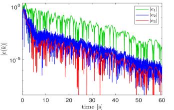
(a) State tracking errors in $\mathcal{S}_{1}$

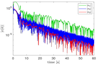
(b) State tracking errors in $\mathcal{S}_{2}$

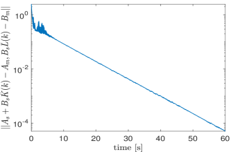
(c) Matching error in $\mathcal{S}_{1}$

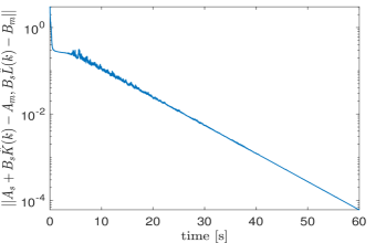
(d) Matching error in $\mathcal{S}_{2}$

Figure 1: State tracking errors and norms of the matching error in $\mathcal{S}_{1}$ and $\mathcal{S}_{2}$.

The two simulations $\mathcal{S}_{3}$ and $\mathcal{S}_{4}$ with constant reference input $r(t)=[0.1\ 0.1\ 0.1\ 0.1]^{\top}\ \forall t\in\mathbb{Z}_{+}$ give the following results. By choosing the stopping criterion (52) with $\varepsilon=10^{-10}$, the simulation $\mathcal{S}_{3}$ stops at $135.02$s, providing the final control gains

$$\hat{K} =\begin{bmatrix}0.0025&0.9383&2.1114\\ 0.0032&0.9843&2.1872\\ -0.0001&-0.1270&-0.3000\\ -0.0008&-0.3070&-0.6931\end{bmatrix}\!,$$

$$\hat{L} =\begin{bmatrix}0.5782&0.3782&-0.7808&0.2464\\ 0.8026&0.5852&0.6704&0.8457\\ 0.0220&0.0451&0.8672&0.2668\\ -0.1724&-0.1077&0.3824&-0.0306\end{bmatrix}$$

with matching error $1.6288\times 10^{-5}$. Such matching error was below $10^{-3}$ at $77.02$s and below $10^{-4}$ at $108.01$s. The simulation $\mathcal{S}_{4}$ stops at $135.03$s, providing the final control gains

$$\hat{K} =\begin{bmatrix}0.0026&0.8951&2.0031\\ 0.0006&0.2586&0.5848\\ -0.0005&-0.2967&-0.6792\\ 0.0013&0.3706&0.8189\end{bmatrix}\!,$$

$$\hat{L} =\begin{bmatrix}0.6298&0.4360&-0.1505&0.4694\\ 0.1389&0.0846&-0.3706&0.0067\\ -0.1010&-0.0410&0.8680&0.1669\\ 0.3353&0.2521&0.5038&0.4175\end{bmatrix}$$

with matching error $1.6992\times 10^{-5}$. Such error was below $10^{-3}$ at $81.81$s and below $10^{-4}$ at $111.88$s. As in $\mathcal{S}_{1}$ and $\mathcal{S}_{2}$, the informative time is $T^{*}=5$ in both $\mathcal{S}_{3}$ and $\mathcal{S}_{4}$. Figures 2(e) and 2(f) illustrate the convergence of the inputs to constant values since the input signals $\hat{K}(t)x(t)+\hat{L}(t)r(t)$ are driven by constant reference input signals.

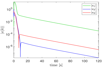
(a) State tracking errors in $\mathcal{S}_{3}$

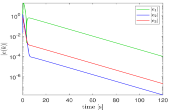
(b) State tracking errors in $\mathcal{S}_{4}$

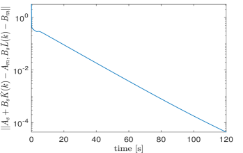
(c) Matching error in $\mathcal{S}_{3}$

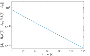
(d) Matching error in $\mathcal{S}_{4}$

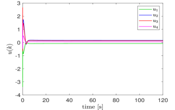
(e) Input signals in $\mathcal{S}_{3}$

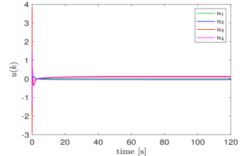
(f) Input signals in $\mathcal{S}_{4}$

Figure 2: State tracking errors, norms of the matching error and input signals in $\mathcal{S}_{3}$ and $\mathcal{S}_{4}$.

As compared to Fig. 1, the results in Fig. 2 exhibit slower convergence, which can be explained with the low excitation provided by a constant reference input. Nevertheless, it is worth mentioning that in all simulations, no matter if the reference input is drawn from a normal distribution or is constant, the sets of data never satisfy the full rank condition (4). Namely, the data collected at the informative time $T^{*}=5$ satisfy

$$\text{rank}\left(\begin{bmatrix}U_{-}(5)\\ X_{-}(5)\end{bmatrix}\right)=5<7,$$

implying that the MRAC problem is solved in scenarios where the collected data do not allow unique identification of the system. In other words, this further confirms that the method proposed in the current paper imposes the least restrictive conditions on data collection compared to existing MRAC methods.

7 Conclusions

In this paper, the MRAC problem has been investigated from a novel perspective of data informativity. Different from previous results on data informativity that used data generated offline, in this paper we have taken an online perspective by verifying data informativity at every time step. A new MRAC method has been developed that ensures convergence of the adaptive gains to a solution of the matching equations, provided such a solution exists. As a preliminary problem, we have analyzed the relationship between data informativity for (unique) system identification and data informativity for model reference control, demonstrating that the former is only sufficient, but not necessary for informativity for model reference control. It becomes necessary only in specific scenarios. Motivated by these findings, we have devised an input function that switches between an adaptive controller and a term that increases the rank of the data matrix. Under the assumption that the matching equations have a solution, this input generates informative data for model reference control after a finite number of time steps. Moreover, in this situation, the adaptive gains of the controller are shown to converge to a solution of the matching equations. As compared to state-of-the-art MRAC approaches, the proposed method does not need knowledge of the input matrix and does not require uniqueness of the solution of the matching equations. A possibility for future research is to explore partial-information scenarios where only input and output data are available.

References

- [1] J. Aseltine, A. Mancini, and C. Sarture, “A survey of adaptive control systems,” IRE Transactions on Automatic Control, vol. 6, no. 1, pp. 102–108, 1958.
- [2] N. T. Nguyen, Model-reference adaptive control. Springer, 2018.
- [3] J. C. Willems, From data to model. Springer Science & Business Media, 2012.
- [4] C. De Persis and P. Tesi, “Formulas for data-driven control: Stabilization, optimality, and robustness,” IEEE Transactions on Automatic Control, vol. 65, no. 3, pp. 909–924, 2019.
- [5] H. J. van Waarde, J. Eising, H. L. Trentelman, and M. K. Camlibel, “Data informativity: a new perspective on data-driven analysis and control,” IEEE Transactions on Automatic Control, vol. 65, no. 11, pp. 4753–4768, 2020.
- [6] M. di Bernardo, U. Montanaro, and S. Santini, “Hybrid model reference adaptive control of piecewise affine systems,” IEEE Transactions on Automatic Control, vol. 58, no. 2, pp. 304–316, 2012.
- [7] S. Kersting and M. Buss, “Direct and indirect model reference adaptive control for multivariable piecewise affine systems,” IEEE Transactions on Automatic Control, vol. 62, no. 11, pp. 5634–5649, 2017.
- [8] S. Yuan, M. Lv, S. Baldi, and L. Zhang, “Lyapunov-equation-based stability analysis for switched linear systems and its application to switched adaptive control,” IEEE Transactions on Automatic Control, vol. 66, no. 5, pp. 2250–2256, 2020.
- [9] J. Xie and J. Zhao, “H-infinity model reference adaptive control for switched systems based on the switched closed-loop reference model,” Nonlinear Analysis: Hybrid Systems, vol. 27, pp. 92–106, 2018.
- [10] R. Franco, H. Ríos, A. F. De Loza, and D. Efimov, “A robust nonlinear model reference adaptive control for disturbed linear systems: An LMI approach,” IEEE Transactions on Automatic Control, vol. 67, no. 4, pp. 1937–1943, 2021.
- [11] G. Guo, J. Kang, R. Li, and G. Yang, “Distributed model reference adaptive optimization of disturbed multiagent systems with intermittent communications,” IEEE Transactions on Cybernetics, vol. 52, no. 6, pp. 5464–5473, 2020.
- [12] D. Yue, S. Baldi, J. Cao, and B. De Schutter, “Model reference adaptive stabilizing control with application to leaderless consensus,” IEEE Transactions on Automatic Control, 2023.
- [13] G. Song and G. Tao, “A partial-state feedback model reference adaptive control scheme,” IEEE Transactions on Automatic Control, vol. 65, no. 1, pp. 44–57, 2019.
- [14] H. Wang, B. Scurlock, N. Powell, A. L’Afflitto, and A. J. Kurdila, “MRAC with adaptive uncertainty bounds via operator-valued reproducing kernels,” IEEE Control Systems Letters, 2023.
- [15] A. M. Annaswamy, A. Guha, Y. Cui, S. Tang, P. A. Fisher, and J. E. Gaudio, “Integration of adaptive control and reinforcement learning for real-time control and learning,” IEEE Transactions on Automatic Control, vol. 68, no. 12, pp. 7740–7755, 2023.
- [16] P. Ioannou and B. Fidan, Adaptive control tutorial. SIAM, 2006.
- [17] M. A. Duarte and K. S. Narendra, “Combined direct and indirect approach to adaptive control,” IEEE Transactions on Automatic Control, vol. 34, no. 10, pp. 1071–1075, 1989.
- [18] S. Boyd and S. S. Sastry, “Necessary and sufficient conditions for parameter convergence in adaptive control,” Automatica, vol. 22, no. 6, pp. 629–639, 1986.
- [19] A. M. Annaswamy and A. L. Fradkov, “A historical perspective of adaptive control and learning,” Annual Reviews in Control, vol. 52, pp. 18–41, 2021.
- [20] E. Lavretsky, “Combined/composite model reference adaptive control,” IEEE Transactions on Automatic Control, vol. 54, no. 11, pp. 2692–2697, 2009.
- [21] G. Chowdhary and E. Johnson, “Concurrent learning for convergence in adaptive control without persistency of excitation,” in 49th IEEE Conference on Decision and Control (CDC), 2010, pp. 3674–3679.
- [22] G. Chowdhary, T. Yucelen, M. Mühlegg, and E. N. Johnson, “Concurrent learning adaptive control of linear systems with exponentially convergent bounds,” International Journal of Adaptive Control and Signal Processing, vol. 27, no. 4, pp. 280–301, 2013.
- [23] N. Cho, H.-S. Shin, Y. Kim, and A. Tsourdos, “Composite model reference adaptive control with parameter convergence under finite excitation,” IEEE Transactions on Automatic Control, vol. 63, no. 3, pp. 811–818, 2017.
- [24] H.-I. Lee, H.-S. Shin, and A. Tsourdos, “Concurrent learning adaptive control with directional forgetting,” IEEE Transactions on Automatic Control, vol. 64, no. 12, pp. 5164–5170, 2019.
- [25] S. B. Roy, S. Bhasin, and I. N. Kar, “Combined MRAC for unknown MIMO LTI systems with parameter convergence,” IEEE Transactions on Automatic Control, vol. 63, no. 1, pp. 283–290, 2017.
- [26] A. Katiyar, S. B. Roy, and S. Bhasin, “Initial-excitation-based robust adaptive observer for MIMO LTI systems,” IEEE Transactions on Automatic Control, vol. 68, no. 4, pp. 2536–2543, 2022.
- [27] G. Tao, “Multivariable adaptive control: A survey,” Automatica, vol. 50, no. 11, pp. 2737–2764, 2014.
- [28] R. R. Costa, L. Hsu, A. K. Imai, and P. Kokotović, “Lyapunov-based adaptive control of MIMO systems,” Automatica, vol. 39, no. 7, pp. 1251–1257, 2003.
- [29] A. K. Imai, R. R. Costa, L. Hsu, G. Tao, and P. V. Kokotovic, “Multivariable adaptive control using high-frequency gain matrix factorization,” IEEE Transactions on Automatic Control, vol. 49, no. 7, pp. 1152–1156, 2004.
- [30] G. Song and G. Tao, “Partial-state feedback multivariable MRAC and reduced-order designs,” Automatica, vol. 129, p. 109622, 2021.
- [31] J. C. Willems, P. Rapisarda, I. Markovsky, and B. L. De Moor, “A note on persistency of excitation,” Systems & Control Letters, vol. 54, no. 4, pp. 325–329, 2005.
- [32] V. Breschi, C. De Persis, S. Formentin, and P. Tesi, “Direct data-driven model-reference control with Lyapunov stability guarantees,” in 2021 60th IEEE Conference on Decision and Control (CDC), 2021, pp. 1456–1461.
- [33] P. Schmitz, T. Faulwasser, and K. Worthmann, “Willems’ fundamental lemma for linear descriptor systems and its use for data-driven output-feedback MPC,” IEEE Control Systems Letters, vol. 6, pp. 2443–2448, 2022.
- [34] G. Pan, R. Ou, and T. Faulwasser, “On a stochastic fundamental lemma and its use for data-driven optimal control,” IEEE Transactions on Automatic Control, vol. 68, no. 10, pp. 5922–5937, 2023.
- [35] H. J. Van Waarde, J. Eising, M. K. Camlibel, and H. L. Trentelman, “The informativity approach: To data-driven analysis and control,” IEEE Control Systems Magazine, vol. 43, no. 6, pp. 32–66, 2023.
- [36] J. Wang, S. Baldi, and H. J. van Waarde, “Necessary and sufficient conditions for data-driven model reference control,” IEEE Transactions on Automatic Control, 2024.
- [37] H. J. van Waarde, “Beyond persistent excitation: Online experiment design for data-driven modeling and control,” IEEE Control Systems Letters, vol. 6, pp. 319–324, 2021.
- [38] M. Rotulo, C. De Persis, and P. Tesi, “Online learning of data-driven controllers for unknown switched linear systems,” Automatica, vol. 145, p. 110519, 2022.
- [39] S. Liu, K. Chen, and J. Eising, “Online data-driven adaptive control for unknown linear time-varying systems,” in 2023 62nd IEEE Conference on Decision and Control (CDC). IEEE, 2023, pp. 8775–8780.
- [40] J. Eising, S. Liu, S. Martínez, and J. Cortés, “Data-driven mode detection and stabilization of unknown switched linear systems,” IEEE Transactions on Automatic Control, 2024.
- [41] B. Zhou and T. Zhao, “On asymptotic stability of discrete-time linear time-varying systems,” IEEE Transactions on Automatic Control, vol. 62, no. 8, pp. 4274–4281, 2017.
- [42] Z.-P. Jiang and Y. Wang, “Input-to-state stability for discrete-time nonlinear systems,” Automatica, vol. 37, no. 6, pp. 857–869, 2001.
- [43] G. Hartmann, M. Barrett, and C. Greene, “Control design for an unstable vehicle,” NASA CR-170393, 1979.
- [44] S. Yuan, B. De Schutter, and S. Baldi, “Robust adaptive tracking control of uncertain slowly switched linear systems,” Nonlinear Analysis: Hybrid Systems, vol. 27, pp. 1–12, 2018.