Unifying Directed and Undirected
Random Graph Models
Abstract
In this paper we explore mathematical tools that can be used to relate directed and undirected random graph models to each other. We identify probability spaces on which a directed and an undirected graph model are equivalent, and investigate which graph events can subsequently be translated between equivalent models. We finally give coupling techniques that can be used to establish an approximate equivalence between directed and undirected random graph models.
As an application of these tools, we give conditions under which two broad classes of random graph models are equivalent. In one of these classes the presence of edges/arcs is determined by independent Bernoulli random variables, while in the other class a fixed number of edges/arcs is placed in between vertices according to some probability measure. We finally use these equivalences to extend a previously established relationship between the directed versions of these model classes to their undirected counterparts.
Keywords Random graphs Random digraphs Model equivalence Coupling
1 Introduction
Since the advent of the original Erdős-Rényi in [13] random graph models have proved paramount for modelling the real world and explaining aspects of network theory. For example, random graph models like the preferential attachment model helped us understand how scale free phenomena emerge in networks (see [2, 5]) while models like the configuration models helped in understanding and controlling disease spread (see [4, 8, 19]).
In many investigations within the field of random graphs, model equivalences prove to be useful tools to investigate the possibilities and limits of specific random graph model instances (see for example [12, 17]). They can be used to put slightly varying random graph models under the same umbrella, as has been done with the Chung-Lu, Norros-Reittu and generalized random graph model (see [1, 11, 21]) in [22], unifying the theory for a class of models. However, they can also be used to make theoretical investigations of models and algorithms easier, which has been done for community detection models in [15] and for biologically motivated network models in [24, 25].
Interestingly, even though model equivalences are well-established in the field, directed and undirected random graph models are often analysed separately. Moreover, the analysis of a directed model often comes after the analysis of a similar undirected model. For example, the inhomogeneous random graph model was treated in [6] far before inhomogeneous random digraphs in [9], and the configuration model was analysed in [20] before the directed configuration model was treated in [10].
Sometimes, this separation of directed and undirected model is merited. This is when the directed model needs to overcome significant complications or generalizations from its undirected counterpart. A telling example is the case of the directed configuration model which needed two intertwined degree sequences in its definition. The nature of these sequences can make its behaviour significantly different from the “normal” configuration model (see [23]). However, there are also cases where the directed model shows very similar behaviour as the undirected model, as was found for inhomogeneous random (di)graphs (compare results in [6] with [9]). This begs the question whether the theory of undirected and directed random graph models can be unified to a certain extend through model equivalences.
This paper aims to establish such unification, by investigating to what extend classes of undirected and directed random graph models can be (expected to be) equivalent. We will start by creating tools to establish equivalence in Section 2. These tools consist of a direct identification of the undirected model that corresponds to a directed model (Theorem 2.4) as well as a coupling technique to show that an undirected model is equivalent to a directed one (Theorem 2.7).
Then, we apply these techniques in Section 3 to show that a previously model equivalence between two directed random graph models can be generalized to their undirected counterparts as well (Theorem 3.5). In this process, we will see that two broad pairs of random graph model classes are equivalent in Section 4. One of these uses independent Bernoulli random variables to generate arcs/edges (like inhomogenious random (di)graphs; see Lemma 4.3), while the other fixes the number of arcs/edges and assigns them vertices based on some conditional measure (like the cell-cell interaction model in [25]; see Lemma 4.4). Finally, these model equivalences will be proven together with other lemmas in Section 5.
2 Equivalence of directed and undirected random graphs
In this section we will provide several notions of equivalence between directed and undirected random graph models. We start by giving a direct equivalence between probability spaces of directed and undirected random graph models. Thereafter, we provide an indirect equivalence that is more useful in practical cases. The proof of our main results can be found in Section 4. In the rest of this paper, we use the term graph to refer to an undirected graph, while digraph will refer to a directed graphs.
2.1 Direct equivalence
While our goal is to establish an relation between graphs and digraphs, it cannot be expected that equivalence always holds. Digraphs inherently encode more information (directionality), so we can only hope to translate between events that do not care about this additional information. For these events, direction might as well be removed; arcs become “normal” edges. Thus, the only events we might wish to translate between, are events that only care about the location of arcs. Given this observation, the natural way to map from a directed to an undirected graph, is forcing the directed graphs to forget the direction of their arcs. We will start by giving the definition of a map on digraphs that achieves this.
Definition 2.1 (Forgetful map).
Let denote the set of simple graphs with vertices, and let denote the set of of simple digraphs with vertices. We define the forgetful map that maps a digraph to a graph as follows:
-
I.
, and
-
II.
.
With Definition 2.1 we can design a random graph model equivalent with a random digraph model by forcing to output whenever outputs . Probabilistically, we can achieve this by mapping the mass of all digraphs from in to the mass of in . This would yields the following direct way to define the “equivalent” undirected model to a directed one.
Definition 2.2 (The forgetful random digraph model).
Given a random digraph model we define the forgetful random digraph model through its probability mass function, by
It turns out that the forgetful random digraph model is the unique model that has the same properties as . Thus, a random graph model can only be equivalent to a random digraph model if is “close” to . This will be formalized as an asymptotic notion. This paper considers three asymptotic notions: deterministic, stochastic, and with high probability. We define these next.
Definition 2.3 (Asymptotic notions).
For a deterministic sequence we mean that as when we write . Similarly, for a random sequence we mean that in probability when we write . Finally, we say a sequence of events occurs with high probability whenever .
To state the main theorem of this section we formalize the concept of an event as a set of simple undirected graphs. The main theorem of this section, whose proof can be found in Section 4.1, is now the following:
Theorem 2.4 (From directed to undirected graphs).
Let be some undirected random graph model, and let be some directed random graph model, both with vertices. For all events we have that
if and only if
Theorem 2.4 states that knowing something about a directed random graph model implies directly that we know something about . However, the main difficulty in applying Theorem 2.4 lies in identifying what looks like through Definition 2.2.
This task is only easy when the probability distribution of a random graph model is known explicitly. However, usually this is not the case: random graph models are often defined indirectly through a random process. In such case identifying undirected counterparts of directed models is cumbersome even for relatively simple digraph models, as the proof of the following corollary illustrates.
Corollary 2.5 (From directed to undirected Gilbert).
Let denote the directed Gilbert model111Note that this model is often referred to in the literature as the Erdős-Rényi model. The model first introduced by Gilbert in [14], while the original model considered by Erdős and Rényi in [13] was the model with a fixed number of edges. with parameters and , and the (undirected) Gilbert model with parameters and . Then it holds that
Proof.
We will apply Theorem 2.4. Hence, we will need to show that the probability mass function of equals that of . Since each arc is placed independently form the other arcs, we have that the probability mass function of for some digraph is given by
Following Definition 2.2, the probability mass function of for an undirected graph is given by
| (1) |
Now, it is important to note that if it has at least one arc in all the same locations as . The mass of each graph in will depend the number of bidirectional arcs that is has. Thus, it is helpful to split (1) up into graphs where we know the number of bidirectional arcs. This yields
If you know there are bidirectional arcs, then we know that . Moreover, each non-bidirectional arc can be placed in either direction between the vertices. So, each term in the sum contributes times to the sum. Finally, we also have to pick where the bidirectional arcs are placed, adding another facter to each term in the sum. Hence, the desired probability becomes
Using Newton’s binomial to compute the sum then yields
This expression equals the mass function of the undirected Gilbert model with parameter . ∎
The previous proof shows that we need better techniques to derive that do not require us to retrieve the probability distribution of a random graph model explicitly. A natural technique that could achieve this, is a coupling, since it allows us to execute the graph generation process from and the digraph generation process from simultaneously. This is what we explore in the next section.
2.2 Indirect and imperfect equivalence
The map is defined through the heuristic that locations of arcs in a digraph and edges in the associated undirected graph should be the same. Therefore, if we can couple the process that generates a random digraph to a process that generates a random graph such that the locations or arcs/edges remain preserved, then we expect to be equal to . We will call such a coupling a location coupling.
Definition 2.6 (Location coupling).
A coupling of a random graph model and a random digraph model is called a location coupling if
It turns out that Definition 2.6 is equivalent to Definition 2.2. This is the subject of the following theorem, which provides a method to indirectly identify . See Section 4.1 for the proof.
Theorem 2.7 (From directed to undirected graphs indirectly).
If there exists a location coupling between two models and , then for all events we have that
Remark.
Although Theorem 2.4 and 2.7 provide exact identifications of , we often do not need an equivalence for all events . Rather, for each specific application a more limited set suffices. These specific events might not care about a fixed number of edges/arcs being placed in different locations. To formalize the extend to which events do not care about wrongly coupled edges/arcs, we introduce the concept of event insensitivity.
Definition 2.8 (Event insensitivity).
Fix an event and a rate . Let be an arbitrary random graph model, and let be derived from the realisation of by adding at most edges, and by removing at most edges. We say that is insensitive for increase at rate if we always have that
Moreover, we say that is insensitive for decrease at rate if we always have that
If both are true, then is completely insensitive at rate .
Remark.
We will not write down the explicit dependence of e.g. on if it is clear from context. Also, while Definition 2.8 is quite strict, for a given random graph model it can be significantly relaxed, depending on the approximate location coupling used and the way errors emerge under the coupling.
Naturally, Definition 2.8 sets an upper-bound for the number of errors that an approximate location coupling is allowed to make. If we can bound this number for specific couplings, then we can use Definition 2.8 to generalise Theorem 2.7. To make this rigorous, we need to define what we mean with coupling errors, and how we count them.
Definition 2.9 (Location coupling errors).
Let be a random graph model and a random digraph model, defined on the same probability space. Consider the following two random variables:
-
– The number of unordered vertex-pairs for which , but .
-
– The number of unordered vertex-pairs for which or , but .
We then define the total number of coupling errors as .
It is often not required to bound the number of location coupling errors deterministically to apply Definition 2.8. Since Theorems 2.4 and 2.7 involve limits of probabilities, bounds on with high probability (cf. Definition 2.3) usually suffice. This can be seen in the following main corollary to Theorems 2.4 and 2.7.
Corollary 2.10 (Approximate location coupling).
Consider a random graph model and a random digraph model coupled on the same probability space. Suppose that happens with high probability and that is insensitive at rate . Then, we have that
Remark.
Note that the complete insensitivity condition in Corollary 2.10 can be weakened to only require insensitivity for increase or decrease if or , respectively.
In the remainder of this paper we will use Corollary 2.10 to couple different classes of random undirected and directed graphs. It will allow us to generalise a previously established equivalence between two classes of digraph models to their undirected counterparts. We will explore this in the next section.
3 Application to model equivalences
Corollary 2.10 translates event probabilities from a directed random graph model to an undirected random graph model. Apart from directly translating limiting results from a directed to an undirected model and vice versa, we can use this corollary to upgrade equivalence relations between directed random graph models to their undirected counterparts. Basically, if we know that for two digraph models and , then Corollary 2.10 would allow us to conclude that for “equivalent” undirected models and .
We will start this section by defining two broad classes of directed and undirected random graph models. The main result of this section is Theorem 3.5, which allows us to extend equivalence between the directed instances of these classes to their undirected counterparts. As an example of this general result, we consider a directed random graph model from [25], motivated by cell-cell interaction networks studied in [24]. We then extend the equivalence on directed graph given in [25] to an equivalence between undirected versions of these models.
3.1 Graphs with independent edge/arc probabilities
The first class of models that we consider, has the main property that edges and arcs are generated independently from one another, possibly after vertices have been given a type. We will assume these types are sampled from some fixed set , and that there is a function that specifies with what probabilities edges/arcs appear. When produced graphs are undirected, we call this model the independent edge graph (IEG). When directed, we will call it the independent arc graph (IAG) model.
Definition 3.1 (Independent edge/arc graphs).
Fix a set and let be a sequence of -dimensional random vectors with entries in such that . Furthermore, fix a function . In the independent arc graph, we generate a digraph by first realising followed by a sequence of independent Bernoulli random variables . We have that if and only if . We denote this model by .
Similarly, for the independent edge graph, we generate a graph by first realising followed by a sequence of independent Bernoulli random variables for each unordered pair . We have that if and only if . We denote this model by .
Remark.
Since generates edges only for each ordered pair , we require to be symmetric. In this needs not be the case.
Since can be any set we want, and since can be any collection derived from , the models IAG and IEG are quite broad. In particular, many well-known random graph models constructed as generalisations of the Gilbert model222Recall this is commonly referred to as the Erdős-Rényi model, and sometimes also called the model. in [14] (cf. Corollary 2.5) fall within the class IAG or IEG. We will give three examples.
Example 3.2 (Independent edge/arc graphs).
For each of the examples we will specify the set , the vector and the probability function .
-
(a)
We can define both the directed and undirected Gilbert model (see [14]) by taking with and setting for some constant .
-
(b)
The geometric inhomogeneous random (di)graph model (see [7]) sets where indicates the -dimensional torus. The vector consists of vertices of the form where and for fixed is sampled according to some distribution on . Finally, satisfies
where are constants and is the -norm on .
- (c)
3.2 Graphs with a fixed number of edges and arcs
The second class of models we consider has the property that the number of arcs/edges is fixed. After generating their vertices, these models repeatedly generate arcs/edges from some underlying distribution without replacement until the required number of arcs is placed. This probability distribution is assumed to be stochastic with respect to the generated vertices, since we want to capture settings where e.g. the placement probability of arcs/edges depends on the number of vertices with a given type. We will name the undirected version of this model the edge selection random graph (ESRG) model, while its directed counterpart is named the arc selection random graph (ASRG) model.
Definition 3.3 (Edge/arc selection random graphs).
Fix a set and let be a sequence of -dimensional random vectors with entries in such that . Also, given , fix a mass function and a number . In the edge selection random graph model, is defined on unordered tuples, while in the arc selection random graph model it is defined on ordered tuples. Given , we realise a (di)graph as follows:
-
1.
Sample and start with .
-
2.
Draw edges/arcs independently from until you hit an edge/arc that is not part of yet.
-
3.
Set , and go back to step 2 until .
We denote the edge selection random graph model by and the arc selection random graph model by .
Remark.
Note from Definition 3.3 that must be symmetric in ESRG, but not necessarily in ASRG.
Through the flexibility in choosing , and , a large body of models are examples of ESRG and ASRG. All these models are some generalisation of the “original” Erdős-Rényi model333Also sometimes referred to as the model. in [13]. Additionally, under certain conditions, edge exchangeable graphs (see [18]) are also examples of Definition 3.3. However, note that in edge exchangeable graphs the number of vertices is not typically fixed. We now give two examples, and later in Section 3.4 we will investigate a third in more detail.
Example 3.4 (Edge/arc selection random graphs).
For each example we specify the set , the random vector and the measure .
-
(a)
We can define both the directed and undirected “classical” Erdős-Rényi model (see [13]) by taking with and setting be the uniform distribution.
-
(b)
We can define (undirected) edge-exchangeable random graphs (see [18]) by setting with , and by fixing a global function . To sample edges we first realize , then construct form by restricting it to and normalizing it with respect to .
Remark.
As the names suggest, it turns out that ESRG and ASRG are related to one another. This relation will be explored in Lemma 4.4 of Section 4.2. Unlike the relation between IEG and IAG, it will now be impossible to derive a direct equivalence through Theorem 2.4 or 2.7. We can only construct an approximate location coupling and use Corollary 2.10 to show equivalence for certain events.
3.3 Extending equivalence from direct to undirected models
Both IAG and IEG are related through Lemma 4.3, and ASRG and ESRG are related through Lemma 4.4. If now a final relationship is established between IAG and ASRG, we can use Corollary 2.10 to upgrade this relationship to IEG and ESRG (and vice versa). This upgrade is important, since relationships between these broad classes of models already exist, and it allows us to gain additional relationships seemingly for free without having to do additional extensive model analyses. To formulate the result, we will first introduce some notation.
Notation.
Given the realization of in and we will set
It must be stressed that and are stochastic quantities, since they depend on . We are now in a position to formulate the main result of this section.
Theorem 3.5 (Directed equivalence to undirected equivalence).
Consider and . Suppose for that there exists a sequence such that
Moreover, let arbitrarily slowly, and suppose is an event insensitive for increase (cf. Definition 2.8) at rate
| (2) |
with high probability. Finally, suppose it is true that
| (3) |
Then, we also have that
| (4) |
with and .
In the final conclusion of Theorem 3.5, note in (4) that and are defined by adding the mass of the directed counterparts of the functions in both possible arc directions. This is logical, since we can only expect to find the equivalent undirected models by adding all the mass at a given location for the directed models; this was the original motivation in Section 2.
3.4 Application to a model for cell-cell interactions
We will end the section with an explicit example showcasing how Theorem 3.5 can transform an equivalence between two directed random graph models into an undirected random graph model. The focal point of the example is motivated by [25] where an equivalence has been established between inhomogeneous random digraphs (Example 3.2(c)) and a model for cell-cell interactions (see [24]). We will first define the model for cell-cell interactions as an example of Definition 3.3.
Example 3.6 (Cell-cell interaction model).
Define the cell-cell interaction model as a special instance of ASRG by setting with elements in of the form , where and is an i.i.d. random variable supported on . To define we set an independent random variable supported on a set with mass function , a function and a function . With these we set
to define
Finally, the model chooses for some fixed . We will denote this model by .
Remark.
Note that this version of the cell-cell interaction models does not follow [25] exactly. Here, self-loops and multi-arcs are not allowed while in the original formulation they are. This discrepancy is alleviated in Lemmas 4.12 and 4.13 of [25], where it is shown that the influence of self-loops and multi-arcs is minimal.
We will now apply Theorem 3.5 to the (directed) models from Example 3.2(c) and Example 3.6. For ease of notation, we will denote the undirected model in Example 3.2(c) as and the directed model in Example 3.2(c) as . Here, is the random variable that samples from and is the kernel of the model.
The main tool that allows us to apply Theorem 3.5 to CCI and IRD is Theorem 3.7 in [25]. We will place stricter assumptions on this model than in [25]. This is to avoid having to repeat the technical arguments of said paper whilst maintaining the essence of applying Theorem 3.5.
Assumption 3.7.
For we require to be supported on and on . We set and define the constants
We assume for all and that .
Because Theorem 3.7 in [25] is formulated in terms of monotone events, we recall their definition before we state the corollary to Theorem 3.5 related to the cell-cell interaction model.
Definition 3.8 (Monotone events).
Let and be two graphs such that . We say a collection of events is increasing if implies . Similarly, we say is decreasing if implies . Finally, we say is monotone if it is either increasing or decreasing.
Corollary 3.9 (CCI to IRG).
Consider such that Assumption 3.7 is satisfied, and define for given types as
Let be a monotone event insensitive at some rate , and suppose there exists a number such that
as for all sequences with satisfying the inequality
| (5) |
for large enough fixed . Then, we also have that
where and is as in Example 3.6, and for .
Remark.
One can upgrade the statement of Corollary 3.9 to and with countably infinite support. However, the statement would become more intricate and the proof more technical. Also, if we compare the exponent in (5) with Theorem 3.7 in [25] we note that it is arbitrary: anything larger than but smaller than zero would suffice.
4 Strategy and proofs of the main results
In this section we will give the heuristics and proofs of the main results. When outlining the strategy, we will provide lemmas that are beneficial for the main results. However, their proofs will be postponed until Section 5.
4.1 Proofs of Theorem 2.4, Corollary 2.5 and Theorem 2.7
To prove Theorem 2.4, two main ingredients are required.
-
1.
We need to show that is the correct model that preserves graph event probabilities. In other words, we need to show that exists.
-
2.
We need to show that graph event probabilities can only be preserved if the undirected random graph model is “close” to . In other words, we need to show that is unique.
The first of these ingredients is covered by the next lemma. Note that it does not provide uniqueness, since it does not rule out the possibility that undirected random graph models exist which asymptotically preserve event probabilities.
Lemma 4.1 ( exists).
The forgetful random graph model (cf. Definition 2.2) is the only undirected random graph model satisfying
for all events .
The second of these ingredients is provided by the following technical lemma. It states that it is not possible for a model different to to asymptotically preserve event probabilities. When no exact coupling exists, there always is an event to which both models assign a different probability.
Lemma 4.2 (No coupling implies event discrepancy).
Suppose and are two sequences of random variables supposted on the same countable set. Suppose for all couplings there exists a constant such that . Then, there exists an event such that
| (6) |
We are now in a position to prove Theorem 2.4. The main technique that combines Lemma 4.1 and 4.2 into a full proof of the theorem, is the maximal coupling theorem (Theorem 2.9 in [16]).
Proof of Theorem 2.4.
Recall that is the total variation distance for graphs. We now tackle the two sides of the equivalence separately, starting with the implication that assumes convergence of the total variation distance.
First implication.
Suppose that . Then, the maximal coupling theorem tells us there exists a coupling such that
| (7) |
Using this coupling we will first use the law of total probability to write
We then rewrite the leftover probability to show that we can remove one of the two events in the intersection with little cost. We find that the leftover intersection probability equals
| (8) |
Now, note that . Thus, we can bound
From (7) we can now conclude that
Substituting this into (8) then shows
Finally, by applying Lemma 4.1 we conclude
Second implication.
Suppose that for all events we have that
while simultaneously we have that . Then, there must exist a constant such that for large enough we have that . From the maximal coupling theorem we then know for any coupling that
Note that both and can be seen as random variables with finite support, since there are only finitely many graphs with a fixed number of vertices. Therefore, due to Lemma 4.2 there must exist an event such that for large
for some . With Lemma 4.1 we then rewrite this as
which directly contradicts the original assumption of this part of the proof. ∎
The proof of Theorem 2.4 relies heavily on the maximal coupling theorem. Thus, if we are able to identify the maximal coupling, then the proof of Theorem 2.4 shows that this is the only coupling mapping random graph models to random digraph models. At the same time, the statement of Theorem 2.7 focusses solely on the location coupling in Definition 2.6). Hence, our strategy to prove Theorem 2.7 will be changing (that is linked to through Definition 2.1) into using a location coupling.
Proof of Theorem 2.7.
Fix an arbitrary event , and under the location coupling define the event . We first note from Definition 2.6 that
| (9) |
Then, by using Definition 2.2, we can write the leftover probability as
Now, because we know that happens, it follows that , and hence we can add the requirement that without altering the probability. Doing this shows
| (10) |
Note that and hence we find, using the law of total probability, that
Substituting this back into (10) yields
through Definition 2.6. Therefore, plugging this result back into (9) shows that
Thus, by Lemma 4.1 we also have that
Since was chosen arbitrarily, we haven proven the theorem. ∎
To derive the result of Corollary 2.10, we observe that event insensitivity (cf. Definition 2.8) implies that we can alter the random digraph model by deleting a certain amount of the arcs, without influencing the probability of the probability of interest. So, if we can construct a location coupling by deleting a limited number of arcs, the result follows form Theorem 2.7.
Proof of Corollary 2.10.
Set . We can start by writing
On the coupled probability space we now know that has at most locations where it differs from . Define by swapping edges from until is matched. Now, we can use the assumed event insensitivity (Definition 2.8) to conclude that
Now, we can remove the even once more (since it occurs with high probability) to conclude that
We next note that under the coupling equals holds for all . In other words, the coupling is a location coupling (Definition 2.6). Hence, we can apply Theorem 2.7 to conclude that
which entails
∎
4.2 Proof of Theorem 3.5 and Corollary 3.9
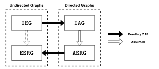
To prove Theorem 3.5 we first recall that we have assumed a relationship between IAG and ASRG. To transform this into a relationship between IEG and ESRG we need to translate events in IEG into events in IAG, and events in ESRG into events in ASRG. This is where Corollary 2.10 comes into play (see Figure 1). The main lemmas needed for the proof specify the rate of event insensitivity we need (cf. Definition 2.8) to apply Corollary 2.10. These lemmas together show how (2) appears in the statement of Theorem 3.5.
The first lemma will link to . Generalizing Corollary 2.5, we might expect that an exact coupling is possible if
However, the final product is usually of lower order than the other terms. Therefore, it is more natural to couple to where . This will yield a coupling error that needs to be counter-balanced with event insensitivity. We will now formulate the coupling lemma.
Lemma 4.3 (Approximate IAG to IEG).
Consider and consider an event that is insensitive for increase at rate with high probability where is some arbitrary function. We have that
where .
Remark.
The maximum with in the formulation of Lemma 4.3 is needed in the edge case where in probability as . Also, note that insensitivity at rate is too strict. Heuristically, this assumes that miss-couplings occur at every location of the graph with the largest possible probability, since for all we have . Although for specific instances of IAG/IEG we can make the insensitivity rate sharper, the formulation we choose yields the easiest universal condition.
The second lemma will translate ASRG to ESRG. Here, we can only resort to an indirect coupling. The idea behind the coupling is that arcs and edges are placed at the same locations; the direction of the arcs does not matter. This coupling would make errors when two arcs are placed between the same vertices (in opposite directions). Then, there is no matching location for the corresponding edge in ESRG. When we have placed arcs already, this coupling error occurs with a probability trivially bounded by . Because we are placing arcs in total, the amount of miss-couplings made is bounded by . This is how the additional event insensitivity appears in (2). We will now formulate the second lemma and subsequently prove Theorem 3.5.
Lemma 4.4 (Approximate ASRG to ESRG).
Consider and suppose there exists a sequence such that and
as . Moreover, suppose with high probability that is insensitive for increase at rate . Then, we have that
where for all .
Remark.
In case of the classical Erdős-Rényi model where edges/arcs are placed, the conditions of Lemma 4.4 would simplify to event sensitivity at any rate as expected. This is because in such setting and .
Proof of Theorem 3.5.
With Theorem 3.5 at our disposal, we now want to use Theorem 3.7 in [25] to prove Corollary 3.9. To do this, we need three additional lemmas with the following purposes:
-
1.
Theorem 3.7 in [25] can only be applied when the events are monotone. Since we will be considering events of the type in the directed setting, we need to show that these are monotone when the input event is monotone.
- 2.
- 3.
We will now formulate the three lemmas that tackle the above purposes.
Lemma 4.5 (Monotonicity preservation).
If is a monotone event, then is monotone too.
Lemma 4.6 (Kernel bound).
Lemma 4.7 (Mass bound).
Note that Lemma 4.6 ensures that for some large enough constant . Hence, the required insensitivity through Lemma 4.3 simplifies to rate for any . Similarly, Lemma 4.7 shows that for large enough . Thus, since we place arcs, the required insensitivity due to Lemma 4.4 only has constant rate. All in all, this show that the total event insensitivity needed has rate for any . This is why said assumption appears in Corollary 3.9, but not in Theorem 3.7 of [25]. Now we will prove the corollary.
Proof of Corollary 3.9.
First, because is insensitive at rate , Lemma 4.3 shows us that
for any that satisfies (5). Hence, since for all , we know that for all satisfying (5) as well. Moreover, given that is a monotone event, we know that is a monotone event too through Lemma 4.5. Thus, we can apply Theorem 3.7 in [25] to conclude that . This shows that (3) is satisfied.
Consider the event for some constant . We know from Lemma 4.6 that happens with high probability on . Similarly, if we set for some , then Lemma 4.7 tells us occurs with high probability on . Now, for every vector in we can choose for some arbitrary to see that
and that
Since happens with probability tending to one, we immediately find that in probability too, and that it is enough to have insensitive at rate to apply Theorem 3.5. Doing this yields
∎
5 Proofs of lemmas
In this section we will present the proofs of the lemmas that were needed for the main results. They will be organized in the same way as the proofs in Section 4. If additional lemmas are needed to prove the lemmas of Section 4, they will be presented here and immediately proven.
5.1 Proof of lemmas in Section 2
To prove Lemma 4.1 we first need to establish some properties of the map (cf. Definition 2.1). We need to show that for all digraph there exists a simple graph such that . Otherwise, potential probability mass from the random digraph model might be missing from . Moreover, we also need to show that for two graphs and the sets and are not overlapping. Otherwise, the mass function of might count the mass from certain digraphs more than once. In the following additional lemma we will show that has the desired properties, after which we will prove Lemma 4.1.
Lemma 5.1 (Properties of the forgetful map).
The following two properties are true:
-
I.
The operator is surjective.
-
II.
For two simple graphs and such that we have that .
Proof.
We will tackle each statement individually.
I.
Let be an undirected simple graph and recall that we identify nodes with their integer-valued label. Define now the corresponding digraph to be the digraph for which if and only if . For this digraph we have that the simple graph has vertex-set which equals by property I of Definition 2.1. We will end by showing that the edge-set equals .
Suppose that , then by construction we have that , and by property II of Definition 2.1 we may conclude that . Similarly, if , then through property II of Definition 2.1 we have that or . From the construction of we know that only and that it must have been created from . Thus, indeed , showing that , meaning is surjective.
II.
If and are two unequal simple graphs, then one of two things must be the case. Either , or (given that ) there exists a vertex-pair such that and or vice-versa. In case the vertex-sets are different property I of Definition 2.1 shows that all graphs in have the vertex-set while all graphs in have vertex-set . In particular, this shows that .
If and , then property II of Definition 2.1 shows that arc or will always be present in the graphs of , while none of these arcs will be present in the graphs of . Hence, we may conclude that . ∎
Proof of Lemma 4.1.
We will first prove that does what we expect of it (existence), and then we show that no other random graph model can do the same (uniqueness).
Existence.
Define the probability mass function of by . We shall define the model through its probability mass function. We set
| (11) |
Note that this is a proper probability mass function. This is because is a probability mass function too, meaning for all graphs , and because
Here, the second equality is due to Lemma 5.1, since property I ensures for all that there exists such that , and since property II ensures that no graph in is double-counted. In the model , we will now rewrite its event probability to find the desired result. We have that
| (12) |
From property II in Lemma 5.1 we know that all the graphs in (12) are unique. Therefore, we get
Uniqueness.
Suppose there exists a model , different from such that
| (13) |
for all events . Then, because is different from , there must be a graph such that . Now, consider the event . We directly find that
This contradicts (13), showing that must be the unique model that preserves graph event probabilities. ∎
We end this section by proving Lemma 4.2. Its proof consists of identifying two events based on the probability mass functions of and of which one must satisfy (6). This is done by showing that the total variation distance between the random variables must converge to zero if (6) is true for both constructed events. This would imply through e.g. Theorem 2.9 in [16] that an asymptotically exact coupling must exist, which the lemma assumes to be false.
Proof of Lemma 4.2.
Define the events and . We will show that (6) holds for at least one of these events. We will prove this by contradiction by assuming that both and as , and subsequently showing that there exists a coupling of and such that .
First from the assumption that does not follow (6) we have that also
| (14) |
Now, since for all we have that , we automatically also have that . Applying a similar reasoning to shows we can rewrite (14) as
We will now rewrite these probabilities as a sum and group them accordingly to find
Next, again by using the definition of , we can conclude that the grouped terms in each sum are positive, so we can write that
| (15) |
We then define the set and note that for each in the joint support of and we must have that , or . Moreover, due to the definition of we must have that
Using this in (15) allows us to conclude that
However, this final expression equals the total variation distance between and . Therefore, since it converges to zero, we may conclude that there exists a coupling of and such that . This is a consequence of e.g. Theorem 2.9 in [16]. All in all, this yields a contradiction with the assumption of the lemma. Therefore, we need to have that for or property (6) is true. ∎
5.2 Proof of lemmas in Section 3
Since all of the lemmas in Section 3 deal with the four broad classes of models, and since all these models first generate a vector before they create a graph, we need to be clear where in the graph generation process we are.
Notation.
We will denote a probability measure for a model conditioned on by . We denote the conditional expectation of a model conditioned on by . The unconditional operators remain and .
Our fist task is proving Lemma 4.3. We will do this by first giving the exact formulation of and then checking how close this is to the IEG formulation in the statement of Lemma 4.3 to identify the required event insensitivity to apply Corollary 2.10. We will first give the lemma that will give us the exact connection between IAG and IEG, after which we will prove Lemma 4.3.
Lemma 5.2 (Exact IAG to IEG).
Consider with some vector and probability function . Define a new probability function as follows:
We have that has the same distribution as .
Proof.
We first note, because is the same in both models, we can consider and to have the same vertex-sets. Now, given the vertices we can couple the graphs in IAG and IEG by coupling the locations of the edges/arcs. For this we define for to be the sequence of edge indicators in . Similarly, we denote by for the sequence of arc indicators in .
Note in both cases that the sequences and are independent, since vertices in have already been sampled. Moreover, every graph outputted by and is captured fully by the sequences and , respectively. Finally, note that will have an edge indicator sequence given by
All in all, if we show an exact coupling between the sequences and , then we have found the location coupling between and , proving the result.
To construct this coupling, we note that is still an independent sequence, because the random vector sequence for is also independent. This is due to the independence in . Moreover, we note that if and only if both and . Therefore,
In other words, we see that the indicators and are the same. Therefore, a location coupling between the two models exists. From Theorem 2.7 it then follows that has the same distribution as . ∎
Proof of Lemma 4.3.
Fix a probability function and choose an arbitrary event insensitive at rate for some diverging function with high probability. We denote the event that has the required insensitivity by . Throughout the proof we will couple the vertex generation processes in all models to be equal. The proof will consist of three main steps:
Step I.
Given , set to be the sequence of edge indicators in , and let be the corresponding sequence in . Since the realized vertices of both models is equal, we note that both sequences are independent, and that has almost the same success probability as , as can be seen in (16). Since each graph is fully determined by its edge sequence after realizing , we will couple both graphs by constructing a coupling of and for fixed , but keeping the sequence of random vectors independent.
The coupling of the the edge indicators in the two models is given by the joint probabilities below.
| (17) |
Note that the marginal probabilities of the indicators indeed coincide with the desired probabilities, and note in particular that a coupling mismatch will ensue only in cases where has edges, but has not. Therefore, (cf. Definition 2.9).
Step II.
Set to be edge set of , the edge set of and the arc set of . Because there exists an exact location coupling between and (by Lemma 5.2), we know in particular that under said coupling it holds that
| (18) |
for all . Therefore, if we chain the coupling established in Step I to the exact location coupling, we can compare to the model . Under this chained coupling, using (18), we find that
Thus, recalling that , we can bound
| (19) |
Now, by (17), takes the value if and only if and . Note for each edge this happens independently with probability conditional on . Therefore, if we set to be an independent sequence, where , we can rewrite (19) as
We will now bound with high probability to prove the lemma.
Step III.
To bound with high probability we compute its expected value and apply the Chernoff bound for binomial random variables (see Theorem 2.21 in [16]). To do this, first note conditioned on that
Using this domination, we hence have that . In particular, this allows us to bound . This bound puts us in a situation where we can apply the Chernoff bound for binomial random variables. Particularly, given the function , we can use Theorem 2.21 in [16] to conclude that
Now, we define the event . Note that , due to the multiplication with , and that
due to the fact that taking the square rook makes the expected value smaller if the maximum is not attained at one. Thus, the previously derived exponential inequalities show that
Step IV.
We will use this final discovery to prove the lemma. First, we will bound using the union bound
| (20) |
Then, note that is insensitive at rate when intersected with , and that the number of coupling-errors is bounded by when intersected with . Therefore, we can use Corollary 2.10 to conclude
| (21) |
Next, we note that , because of the assumption in Lemma 4.3, and that , du to the conclusion in Step III. Substituting this together with (21) into (20) yields
Now, the final thing we need to do to prove the lemma, is changing into . We can do this analogously to the way we have introduced these events by making the following two bounds
Recalling that and indeed shows that
∎
Now, we move on to prove Lemma 4.4. As stated in Section 4.2, we will prove this lemma by providing an explicit coupling between ASRG and ESRG and counting how many errors this coupling makes. The idea behind the coupling is to place as much edges between vertices in ESRG that have arcs in ASRG and whenever this is not possible to pick a random pair of vertices. We start by defining the coupling.
Definition 5.3 (Approximate location coupling ASRG vs. ESRG).
Sample a vector and a (directed) mass function on . Also, define the (undirected) mass function from by setting . From these objects we will generate two graphs: a directed graph and an undirected graph with arc/edges.
We build both graphs one arc/edge at a time, where follows the building algorithm of in Definition 3.3. The graph will be built simultaneously according to the following three rules:
-
I.
If arc is generated in , and the edge in already exists, then generate a new edge in according to the procedure in rule III.
-
II.
If arc is generated in , and the arc does not exist yet, then generate in .
-
III.
If in the arc is generated in , and the arc already exists, then generate an edge in by sampling edges independently from until a non-existing edge is found.
Before we can analyse the coupling, we first need to show that Definition 5.3 is a proper coupling between and . To do so, note that an edge gets sampled proportional to in rule II, since both arcs and might lead to edge . Additionally, rule I and III will trivially generate an edge proportional to . To make these observations formal, we state and prove an auxiliary lemma.
Lemma 5.4 (ESRG and ASRG coupling exists).
The procedure specified in Definition 5.3 is a coupling between and .
Proof.
Start for both models by generating the same vertex type vector . We then note that graph in Definition 5.3 will trivially follow the generation procedure of . To show follows the generation procedure of we will inductively generate an arc in and show that the corresponding edge generated in will have the same probability as an edge being sampled according to the procedure in Definition 3.3.
Base case.
As our base case we will generate the first edge/arc pair. Since no edges or arcs have been generated yet, we note that only rule II could apply. In this case, the edge in will be generated if and only if either the arc or the arc is generated in . This event will happen with probability . Therefore, when generating the first edge/arc-pair the marginal probabilities in both models are still respected.
Induction step.
Suppose that arcs/edge-pairs have already been generated, and assume marginally both graph and follow the procedure in Definition 3.3. We will consider the generation of arc . For this, denote by the set of already generated arcs in , and denote by the set of occupied edge locations, viewed from the perspective of . In other words, . We will now check whether the procedure in Definition 3.3 is still respected when either of the rules in Definition 5.3 is invoked.
Note that the only interesting rule to check is rule II, since in both rule I and III the edge generated in is independent from the arc generated in . Moreover, the generated edge in has probability proportional to the remaining mass in . Therefore, these rules will trivially satisfy Definition 3.3.
Now, if the rule II is invoked, we note that either of the arcs and will result in the generation of in . Therefore the raw mass of is, similar to the base case, given by . However, when rule II is invoked, we are conditioning on the event that the generated arc in does not come from the set . Therefore, since arcs from and are off-limits in the arc-generation process in this step, the probability of being generated in under rule II is
| (22) |
Now, the idea is to transform the mass function in the denominator into the function . To do this, we will define to be a set of unordered pairs of vertices from . Using this definition, noting that contains arc if and only if it contains , we may rewrite (22)
Note that is exactly the set of occupied edges in . Thus, the probability that gets generated under rule I is given by , normalised over the masses of the leftover edges that can be chosen, as required in . Finally, this means that the marginals of and in Definition 5.3 indeed follow the rules in Definition 3.3. ∎
Lemma 5.4 ensures that we have found a coupling that we can use in Corollary 2.10 to specify the rate of event insensitivity needed to translate between ASRG and ESRG. To calculate the rate, we need to establish a high probability bound on the number of times there is a location with an edge in but no arc in and vice versa under the coupling in Definition 5.3. To do this, we consider the coupling as a dynamic process, and note that the number of (location) miss-couplings only increases when rule III is invoked; in rule II the arc and edge are matched exactly, and in rule I a miss-match is both created and resolved.
We will first specify the process which counts miss-coupled edges/arcs under Definition 5.3 as the graphs are constructed. Thereafter, we will identify exactly when miss-couplings occur and show that this process induces a super-martingale. This will allow us to compute properties of the error counting process more easily.
Definition 5.5 (Error process).
Consider the process in Definition 5.3 and denote by and the intermediate graphs after arcs have been generated. Denote by the number of location coupling errors between these graphs. This is the number of times that an edge is present in , but both and are not present in together with the number of times or is present in , but is not present in .
Remark.
Note for fixed and that , since we have found all coupling-errors in the graph once all edges/arcs have been placed.
Lemma 5.6 (Conditional error process).
We have that is the indicator that rule III is invoked when generating arc/edge in Definition 5.3.
Proof.
We first note that whenever rule II is invoked no coupling error is created, since both arcs are placed at the same locations. Thus, under the execution of rule II we have that . Next, we see that rule III will create exactly one additional error. This is, because in the undirected model an additional edge is placed, while in the directed version of the model a bidirectional arc is created. This bidirectional arc is in the same location as a previously placed edge. Therefore, the newly generated edge in the undirected version of the model forms the coupling-error. This means that when rule III is invoked.
Finally, note when rule I is invoked both a new miss-coupling is created, while another one is resolved. Since an arc is generated in the same place as an already existing edge, that miss-coupling is resolved, reducing the number by one. However, since we are also placing an additional edge, we are creating a new miss-coupling as well. We know that this new edge cannot be generated in a location where there already is an arc in the directed version of the model, since from rules I–III we see that arcs are only generated at locations where edges already exist (or an edge is immediately placed at the same location). Thus, we see that in case of rule I we have that . All in all, we see that only the application of rule III will increase the number of miss-couplings by one. Therefore, given is the indicator that rule III is invoked. ∎
Lemma 5.7 (Error super-martingale).
Consider conditioned on . We have that the process given by
is a conditional super-martingale given . Here, the sequences and are given by
Proof.
The proof will consist of the following two steps:
-
I.
We will find an upper-bound on probability of increasing by one given .
-
II.
We use this to prove that is a super-martingale.
A general observation we will often use through the proof, is the fact that for all .
Step I.
From Lemma 5.6 it follows that at step , given the value of , an additional coupling error is made only when rule III needs to be invoked. Note that this rule is only invoked when an arc gets generated at the same location as an already generated arc, creating a bidirectional arc. If we denote by the set of already placed arcs after arc generation steps, then we define as the set of arcs that have not yet become a bidirectional arc. Under these definitions, we can write the probability of creating a bidirectional arc when generating arc number as
Now, note that since arcs have been placed. Moreover, note that . The factor two appears, since each coupling error (cf. Definition 5.5) corresponds to a bidirectional arc by Lemma 5.6. Both these arcs need be removed from to find . Using this, we find the following error upper-bound at step :
Step II.
Denote by the indicator that rule III had to be executed when generating arc/edge-pair . From the result of Step I we know that conditional on we have that . Using both these facts we will now compute for fixed , establishing the martingale property. For this we note that is in the sigma algebra generated by , since it is only off-set by deterministic constants. Therefore, we can rewrite
where we used Lemma 5.6 for the last step.
Next, using the previously established conditional stochastic domination, we upper-bound the conditional expectation as
| (23) |
Now, we note that we can rewrite the sum and product combination as follows:
Substituting it into (23) then yields
Finally, we rewrite the leftover experssion by factoring the -term and find the desired result
∎
Remark.
Note that is a “regular” martingale if and only if for some constant . This is only possible when , which corresponds to a case where we sample edges/arcs uniformly at random. The only model in which this happens, is the classical (directed) Erdős-Rényi model.
Having established the super-martingale through Lemma 5.7, we are now in a position to prove Lemma 4.4 using Corollary 2.10. The proof will mainly consist of deriving a high-probability bound on by applying the martingale maximal inequality, and then using this bound in the application of Corollary 2.10. Before presenting the proof of Lemma 4.4, we will formulate and prove one final auxiliary lemma that bounds the growth speed of the martingale by a simpler expression (which equals the required event insensitivity rate in the statement of Lemma 4.4).
Lemma 5.8 (Martingale growth speed).
Assume that for some function . We have that
Proof.
First, by noting that and that we can bound the sum as
Then, by computing the product and reversing the order of the sum, we find that the upper bound equals a partial sum of the geometric series.
Next, we will apply Bernoulli’s inequality in the numerator of the previously derived upper-bound to find an expression close to the desired result.
Finally, since we know that for large we will have that . Thus, we obtain the desired result:
∎
Proof of Lemma 4.4.
First, given a coupled directed and undirected random graph model, we recall that is the number of unordered vertex pairs and such that is present in the undirected model, but both and is not in the directed model. Similarly, are the number of instances where or is present in the directed model, but is not in the undirected model. See Definition 2.9.
Consider and for which we couple the vectors to be equal. The proof boils down to first noting that by Definition 5.3, and then bounding (cf. Definition 5.5). We analyse through the maximal inequality (see [3]; Theorem 5.3). After we do this, we use Corollary 2.10 under the coupling specified in Definition 5.3. We can do this, because Lemma 5.4 guarantees Definition 5.3 is a correct coupling between and . The proof will now have the following two steps:
-
I.
Conditioned on , we will bound .
-
II.
We use this to prove the statement of the lemma.
Step I.
Recall the definition of the sequences , and the super-martingale from Lemma 5.7. The maximal inequality on shows for any constant that
| (24) |
where . Note that is stochastically increasing in with . Therefore, we can bound and as follows:
Now, we set for some sequence . With this, we can find a bound on the growth of using (24).
Here, the final inequality is due to Lemma 5.8 when taking . Note that this upper-bound implies that .
Step II.
Fix an , and define the events , and . We start by bounding the desired probability using the union bound as
| (25) |
Similar to the proof of Lemma 4.3 we note that intersected with and the event has the desired event insensitivity to apply Corollary 2.10. Thus, applying it yields
| (26) |
At the same time, we have that , due to the assumptions in Lemma 4.4. Moreover, we can bound
Here, , due to the assumptions that in probability. Moreover, the fact that is due to Part I, which is true for any vector . Substituting this back into (25) with (26) shows for large enough that
Through an analogous approach to Part IV of the proof of Lemma 4.3 we will remove the extra intersections in this final inequality to find
Finally, because this is ture for any we indeed have that
∎
We end this section by proving Lemmas 4.5 through 4.7. These were the lemmas needed to prove Corollary 3.9 with Theorem 3.5.
Proof of Lemma 4.5.
Without loss of generality we will only show that being increasing implies is increasing too. Consider a digraph and suppose . Because is a marked sub-graph of we know that has arcs in locations were has arcs too. Therefore, we have .
Now, by definition implies that . Since is increasing, we have that implies too. However, by definition that entails too. Therefore, we indeed find that is increasing. ∎
Proof of Lemma 4.6.
Proof of Lemma 4.7.
Because of Assumption 3.7 for each there will be at least one such that . A similar thing is true for each . Now, if an arc is generated in then it will be generated proportional to . In other words, the maximum of given will be dictated by the minimum of . By nothing both and are at their core sets of vertices with specific types drawn from . If we set , then we note that each individual and is stochastically bounded from below by a random variable.
We will now consider the event where one of the values or is “too small” and show this cannot happen. Specifically, we are interested in
We will show that happens with high probability on , and subsequently that is sufficiently bounded when . First, applying a union bound on the compliment of , and applying the aforementioned stochastic domination, gives us
Then, by applying the Chebyshev inequality we find indeed that
Thus, happens with high probability. Finally, for every in we have for all and that . Therefore, for these vectors we may bound
∎
Acknowledgments.
The research of Mike van Santvoort is funded by the Institute for Complex Molecular Systems (ICMS) at Eindhoven University of Technology.
References
- [1] William Aiello, Fan Chung, and Linyuan Lu. A random graph model for power law graphs. Experimental Mathematics, 10(1):53–66, 2001.
- [2] Réka Albert, Hawoong Jeong, and Albert-László Barabási. Diameter of the World-Wide Web. Nature, 401:130–131, 1999.
- [3] Paolo Baldi. Stochastic Calculus: An Introduction Through Theory and Exercises. Springer Nature, Cham, first edition, 2017.
- [4] Frank Ball and David Sirl. Evaluation of vaccination strategies for SIR epidemics on random networks incorporating household structure. Journal of Mathematical Biology, 76(1-2):483–530, 1 2018.
- [5] Albert-László Barabási and Réka Albert. Emergence of Scaling in Random Networks. Science, 286(5439):509–512, 1999.
- [6] Béla Bollobás, Svante Janson, and Oliver Riordan. The phase transition in inhomogeneous random graphs. Random Structures and Algorithms, 31(1):3–122, 8 2007.
- [7] Karl Bringmann, Ralph Keusch, and Johannes Lengler. Geometric inhomogeneous random graphs. Theoretical Computer Science, 760:35–54, 2 2019.
- [8] Tom Britton, Svante Janson, and Anders Martin-Löf. Graphs with Specified Degree Distributions, Simple Epidemics, and Local Vaccination Strategies. Advances in Applied Probability, 39(4):922–948, 2007.
- [9] Junyu Cao and Mariana Olvera-Cravioto. On a general class of inhomogeneous random digraphs. Random Structures & Algorithms, 56(3):722–774, 5 2019.
- [10] Ningyuan Chen and Mariana Olvera-Cravioto. Directed Random Graphs with given Degree Distributions. Stochastic Systems, 3(1):147–186, 6 2013.
- [11] Fan Chung and Linyuan Lu. Connected Components in Random Graphs with Given Expected Degree Sequences. Annals of Combinatorics, 6:125–145, 2002.
- [12] F. den Hollander, M. Mandjes, A. Roccaverde, and N. J. Starreveld. Ensemble equivalence for dense graphs. Electronic Journal of Probability, 23, 2018.
- [13] P. Erdős and A. Rényi. On random graphs I. Publicationes Mathematicae Debrecen, 6:290–297, 1959.
- [14] E.N. Gilbert. Random graphs. The Annals of Mathematical Statistics 1, 30:1141–1144, 1959.
- [15] Martijn Gösgens, Remco van der Hofstad, and Nelly Litvak. The projection method: a unified formalism for community detection. Frontiers in Complex Systems, 2, 2 2024.
- [16] Remco van der Hofstad. Random Graphs and Complex Networks, volume 1. Cambridge University Press, Cambridge, 2016.
- [17] Svante Janson. Asymptotic equivalence and contiguity of some random graphs. Random Structures and Algorithms, 36(1):26–45, 1 2010.
- [18] Svante Janson. On Edge Exchangeable Random Graphs. Journal of Statistical Physics, 173(3-4):448–484, 11 2018.
- [19] Svante Janson, Malwina Luczak, and Peter Windridge. Law of large numbers for the SIR epidemic on a random graph with given degrees. Random Structures and Algorithms, 45(4):726–763, 12 2014.
- [20] Michael Molloy and Bruce Reed. The Size of the Giant Component of a Random Graph with a Given Degree Sequence. Combinatorics Probability and Computing, 7(3):295–305, 1998.
- [21] Ilkka Norros and Hannu Reittu. On a conditionally Poissonian graph process. Advances in Applied Probability, 38(1):59–75, 3 2006.
- [22] Henri Van Den Esker, Remco Van Der Hofstad, and Gerard Hooghiemstra. Universality for the distance in finite variance random graphs. Journal of Statistical Physics, 133(1):169–202, 10 2008.
- [23] Pim van der Hoorn. Degree-Degree Correlations and Directed Paths. PhD thesis, Universiteit Twente, Enschede, 2016.
- [24] Mike van Santvoort, Óscar Lapuente-Santana, Maria Zopoglou, Constantin Zackl, Francesca Finotello, Pim van der Hoorn, and Federica Eduati. Mathematically mapping the network of cells in the tumor microenvironment. Cell Reports Methods, 5, 2 2025.
- [25] Mike van Santvoort and Pim van der Hoorn. From inhomogeneous random digraphs to random graphs with fixed arc counts, 9 2023.