Recent Advances in Numerical Solutions for Hamilton-Jacobi PDEs

Abstract

Hamilton-Jacobi partial differential equations (HJ PDEs) play a central role in many applications such as economics, physics, and engineering. These equations describe the evolution of a value function which encodes valuable information about the system, such as action, cost, or level sets of a dynamic process. Their importance lies in their ability to model diverse phenomena, ranging from the propagation of fronts in computational physics to optimal decision-making in control systems. This paper provides a review of some recent advances in numerical methods to address challenges such as high-dimensionality, nonlinearity, and computational efficiency. By examining these developments, this paper sheds light on important techniques and emerging directions in the numerical solution of HJ PDEs.

1 Introduction

Hamilton-Jacobi partial differential equations (HJ PDEs) are foundational mathematical tools that arise in diverse areas such as optimal control, geometric optics, and computational physics [30, 5, 22]. These equations are commonly written in the form

$$\begin{dcases}\partial_{t}{S}(x,t)+H(\nabla_{x}{S}(x,t),x,t)=0,&x\in\Omega,t>0,\\ S(x,0)=J(x),&x\in\Omega,\end{dcases}$$ (1)

where $S(x,t)$ is the value function, $H$ is the Hamiltonian encoding the system’s dynamics, $J(x)$ represents the initial condition, and $\Omega\subseteq\mathbb{R}^{n}$ is the spatial domain. If $\Omega$ is a bounded domain, certain boundary conditions are imposed on $S$. If $\Omega$ is the whole space $\mathbb{R}^{n}$, the value $S(y,T-t)$ is the optimal value of the following optimal control problem:

$$\min\left\{\int_{t}^{T}L(u(s),x(s),s)ds+J(x(T))\colon\dot{x}(s)=f(u(s),x(s),s)\;\forall s\in[t,T],x(t)=y\right\},$$ (2)

where $u$ is the control function taking value in $\mathbb{R}^{m}$. In these two problems, the running cost $L$, the dynamical source term $f$, and the Hamiltonian $H$ are connected by

$$H(p,x,t)=\sup_{u\in\mathbb{R}^{m}}\{-\langle p,f(u,x,T-t)\rangle-L(u,x,T-t)\}.$$

HJ PDEs are notable for their ability to capture complex dynamics in high-dimensional and nonlinear systems [33, 63]. They are central to modeling phenomena such as the propagation of wavefronts [58], the computation of geodesics, and decision-making in optimal control problems [5]. Despite their theoretical significance and wide applicability, solving HJ PDEs efficiently, especially in high dimensions, remains a challenging task, particularly in high-dimensional settings, where traditional grid-based methods face the curse of dimensionality [7, 55].

Recent years have seen significant progress in the development of numerical methods for solving HJ PDEs. These advances have been driven by the need for computationally efficient, accurate, and scalable algorithms to tackle high-dimensional problems and non-smooth solutions [28]. Techniques leveraging variational principles [17], level-set methods [58], and modern machine learning [48, 54, 65] have opened new avenues for addressing these challenges.

This paper reviews some of the recent advances in numerical methods for HJ PDEs, highlighting their theoretical underpinnings, practical implementations, and limitations. We review a series of approaches including grid-based methods (Section 2), methods based on representation formulas (Section 3), Monte-Carlo-based methods using Laplace’s Method (Section 4), and Deep Learning methods (Section 5). While not comprehensive, our review of these developments aims to provide insights into the current numerical landscape and to identify promising directions for future research.

2 Grid-based Methods

Grid-based numerical methods have been the cornerstone of computational approaches for solving HJ PDEs [21, 58, 59, 50, 3, 66]. Recent advances have focused on improving accuracy, computational efficiency, and handling of discontinuities in the solution gradients. This section provides an overview of some key developments in grid-based methods over the past decade. For a more comprehensive review of grid-based numerical methods for HJ PDEs, we refer to [31].

2.1 High-Order ENO and WENO Schemes

While monotone schemes [21, 58, 59] are inherently limited to first-order accuracy, high-order Essentially Non-Oscillatory (ENO) schemes [67] and their Weighted ENO (WENO) variants [50] have been developed to achieve uniform high-order accuracy in smooth regions while robustly capturing discontinuities in derivatives. In the context of one-dimensional finite difference methods for solving HJ PDEs (1), for simplicity consider the case where $H(\nabla_{x}{S}(x,t),x,t)=H(\nabla_{x}{S}(x,t))$, the ENO or WENO method takes the form

$$\dfrac{d}{dt}S_{i}+\hat{H}(p_{i}^{-},p_{i}^{+})=0,$$

where $S_{i}$ approximates the value of $S(x_{i},t)$. Here $\hat{H}(\cdot)$ is a monotone Hamiltonian and $p_{i}^{-},p_{i}^{+}$ represents the approximation to the derivative $S_{x}(x_{i},t)$ computed with stencils biased to the left and right, respectively. For ENO scheme, the approximation of $p_{i}^{-}$ starts with a stencil containing only $\{S_{i-1},S_{i}\}$, then the ENO method adaptively extends this stencil by adding points that yield the “smoothest” local reconstruction, thereby avoiding interpolation across discontinuities, until the desired number of points has been reached. In the end, a single, optimally chosen stencil is used to approximate the term $S_{x}^{-}(x_{i},t)$. As for WENO scheme, it forms a convex combination of candidate approximations computed on several stencils. A typical approximation to the spatial derivatives can be written as:

$$S_{x}^{-}(x_{i},t)=\sum_{k=0}^{r-1}\omega_{k}\hat{S}_{x_{i}}^{k},\quad\omega_{k}=\frac{\alpha_{k}}{\sum_{l=0}^{r-1}\alpha_{l}},\quad\alpha_{k}=\frac{d_{k}}{(\epsilon+\beta_{k})^{p}},$$

where $\hat{S}_{x_{i}}^{k}$ is the $k$-th stencil approximation of $S_{x}^{-}(x_{i},t)$, $\omega_{k}$ are non-linear weights satisfying $\sum_{k=0}^{r-1}\omega_{k}=1$. The coefficients $d_{k}$ are the linear weights that form the approximation $\sum_{k=0}^{r-1}\omega_{k}\hat{S}_{x_{i}}^{k}$ as the $r$-th degree polynomial reconstruction over the full stencil. $\beta_{k}$ are smoothness indicators that measure the local variation of the solution, and $\epsilon$ is a small positive number to avoid division by zero. Based on the spatial discretizations discussed above, time discritization can be performed using either explicit total variation diminishing Runge–Kutta methods or multi-step schemes. Hermite polynomials are used to develop Hermite-type WENO schemes for solving HJ PDEs [64, 75].

These methods have undergone continuous refinements to improve their performance, robustness, and computational efficiency. Significant advances in WENO methodology include the development of exponential polynomial-based schemes by [40], achieving third-order accuracy with improved handling of discontinuities. In the same year, [2] introduced innovative RBF-ENO/WENO schemes combined with Lax-Wendroff type time discretizations, demonstrating superior performance for problems with complex solution structures. Recent efforts have emphasized adaptivity and computational efficiency. In [1], a fifth-order WENO scheme based on Legendre polynomials is constructed for simulating HJ equations in a finite difference framework. Most recently, [74] introduced a third-order, fifth-order, and seventh-order finite difference ghost multi-resolution WENO (GMR-WENO) schemes that only utilize the information defined on one four-point, one six-point, or one eight-point spatial stencil for designing high-order spatial approximations without introducing any other smaller stencils.

2.2 Discontinuous Galerkin Methods

The discontinuous Galerkin (DG) finite element method is a flexible, high-order finite element method using discontinuous piecewise polynomial spaces for both the numerical solution and test functions [20]. DG methods are developed for solving the derivatives in the HJ PDEs in [38, 46] and then recover the solution from its derivatives. In [13, 47, 14], DG methods are applied to directly approximate the solution variable. Local DG methods are studied in [72]. An adaptive sparse grid local DG method is introduced in [36] for solving HJ equations in high-dimensional setup. The alternating evolution DG method proposed in [49] is based on an alternating evolution system for the HJ equation and achieves high order accuracy. In [43], an arbitrary Lagrangian–Eulerian local DG method is developed for HJ equations, leveraging a time-dependent approximation space defined on a moving mesh.

3 Solutions Based on Representation Formulas

For certain classes of HJ PDEs, viscosity solutions can be efficiently computed using representation formulas. A key advantage of this approach is that it transforms the problem of solving a PDE into an optimization problem, which helps mitigate the curse of dimensionality. In this section, we focus on HJ PDEs defined on the entire space $\Omega=\mathbb{R}^{n}$ and explore how these representation formulas leverage intrinsic problem structures, such as constant or piecewise constant velocities or momenta, to facilitate computation.

Firstly, we consider the case when the Hamiltonian only depends on the momentum $\nabla_{x}S$. In this case, the viscosity solution has two representation formulas, namely Lax-Oleinik and Hopf formula [6]. When the Hamiltonian $H$ is convex, the solution is given by the Lax-Oleinik formula

$$S(x,t)=\inf_{u\in\mathbb{R}^{n}}\left\{J(u)+tH^{*}\left(\frac{x-u}{t}\right)\right\},$$ (3)

where in the remainder of this paper, we denote by $f^{*}$ the Fenchel–Legendre transform of a convex lower-semicontinuous function $f$, defined by $f^{*}(p)=\sup_{x\in\mathbb{R}^{n}}\{\langle x,p\rangle-f(x)\}$. On the other hand, when the initial condition $J$ is convex, the solution is given by the Hopf formula

$$S(x,t)=\sup_{p\in\mathbb{R}^{n}}\left\{\langle x,p\rangle-tH(p)-J^{*}(p)\right\}.$$ (4)

These formulas can be used to compute the viscosity solution at a given point $(x,t)$ by solving an optimization problem. In this way, the algorithm can mitigate the curse of dimensionality. Moreover, the value on each point is independent from each other, making the computation easy to parallel. When the Hamiltonian is 1-homogeneous, [28] designed fast solver by using the split Bregman iterative method to solve these two representation formulas. Later, in [45], the authors use these formulas to compute the redistancing problem, which, after using the level set method, can be solved by solving an Eikonal equation. In Fig. 1 we show a numerical result in [28] where the initial condition is $J(x)=\frac{1}{2}\|x\|_{1}^{2}$ and the Hamiltonian is $H(x)=\sqrt{\langle x,Dx\rangle}$ with certain diagonal positive definite matrix $D$.

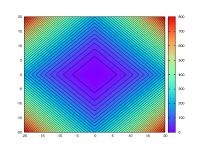
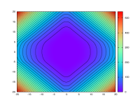
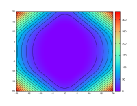
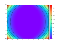
Figure 1: Evaluation of the solution $S((x_{1},x_{2},0,0,0,0,0,0)^{T},t)$ of the HJ-PDE with initial data $J=\frac{1}{2}\|\cdot\|_{1}^{2}$ and Hamiltonian $H=\|\cdot\|_{D}$, for $(x_{1},x_{2})\,\in\,[-20,20]^{2}$ for different times $t=0,5,10,15$.

The Hopf representation formulas are further generalized to linear dynamics, which is proposed as a future direction in [28] and then developed in [42]. To be specific, they consider the class of optimal control problems with linear dynamics in the following form

$$\nu(y,t)=\min\left\{\int_{t}^{T}L(u(s),s)ds+J(x(T))\colon\dot{x}(s)=Ax(s)+B(s)u(s)\>\forall s\in[t,T],x(t)=y\right\}.$$

The function $x,t\mapsto\phi(x,t)=\nu(x,T-t)$ solves the HJ PDE with initial condition $J$ and the Hamiltonian defined by

$$\begin{split}H(x,p,t)&=\sup_{u\in\mathbb{R}^{m}}\{-\langle p,Ax+B(T-t)u\rangle-L(u,T-t)\}=-\langle p,Ax\rangle+\sup_{u\in\mathbb{R}^{m}}\{\langle-B(T-t)^{T}p,u\rangle-L(u,T-t)\}\\ &=-\langle p,Ax\rangle+L^{*}(-B(T-t)^{T}p,T-t),\end{split}$$

where $L^{*}(\cdot,t)$ is the Fenchel-Legendre transform of $L(\cdot,t)$. To solve the HJ PDE and the corresponding optimal control problem, a change of variable $z(t)=e^{-tA}x(t)$ is applied to the optimal control formulation to get

$$\nu(y,t)=\min\left\{\int_{t}^{T}L(u(s),s)ds+J(e^{TA}z(T))\colon\dot{z}(s)=e^{-sA}B(s)u(s)\;\forall s\in[t,T],z(t)=e^{-tA}y\right\}.$$

After setting $\tilde{\nu}(e^{-tA}y,t)=\nu(y,t)$, the function $x,t\mapsto\tilde{\phi}(x,t)=\tilde{\nu}(x,T-t)$ solves the HJ PDE with an initial condition $z\mapsto\tilde{J}(z):=J(e^{TA}z)$ and Hamiltonian

$$\tilde{H}(p,t)=\sup_{u\in\mathbb{R}^{m}}\left\{-\langle p,e^{-(T-t)A}B(T-t)u\rangle-L(u,T-t)\right\}=L^{*}(-B(T-t)^{T}e^{-(T-t)A^{T}}p,T-t).$$

In this case, the Hamiltonian $\tilde{H}$ only depends on the momentum variable $p$ and the time variable $t$. Therefore, the viscosity solution to the HJ PDE can be represented by the generalized Hopf formula:

$$\tilde{\phi}(x,t)=-\min_{p\in\mathbb{R}^{n}}\left\{\tilde{J}^{*}(p)+\int_{0}^{t}H(p,s)ds-\langle x,p\rangle\right\},$$

which is solved by discretizing over time axis and then applying some optimization method, such as a relaxed Newton’s method in [42]. Moreover, in [42] the authors also studied differential games with linear dynamics, which corresponds to more complicated non-convex Hamiltonians. Following this line, in [15, 16, 41], different optimization methods, such as primal-dual method or coordinate descent method, have been applied to the generalized Hopf formula to solve more complicated non-convex Hamiltonians or differential game problems. More complicated problems have been solved with a more general form of Hopf formula, such as HJ PDEs with state-dependent non-convex Hamiltonian [17], and HJ equation in density spaces [18].

Besides these general formulas, some other special cases are studied. For instance, [12] proposes the representation formula for the class of HJ PDEs with Hamiltonian in the form of $H(p,x)=K(p)-\frac{1}{2}(x-v_{0})^{T}M(x-v_{0})$ for piecewise affine positively 1-homogeneous convex function $K$, symmetric positive definite matrix $M$, and a vector $v_{0}\in\mathbb{R}^{n}$, with assumptions relating $M$ to the level set of $K$. These HJ PDEs correspond to optimal control problems with a quadratic running cost on the state variable and a rectangular constraint on velocity, which makes the optimal trajectory in a piecewise linear form. Then, the viscosity solution can be represented by a minimization problem of a piecewise third order polynomial function adding with the initial condition. The dual case is presented in [11], which considers the HJ PDEs with Hamiltonian $H(p,x)=\frac{1}{2}\langle p,Mp\rangle-U(x)$, where $U$ is a positive 1-homogeneous convex function whose level set is determined by the matrix $M$. This corresponds to the optimal control problem with running cost to be a combination of kinetic energy and potential energy $U$. Under these assumptions, the optimal trajectory is a piecewise quadratic function, and the viscosity solution to the HJ PDE is a supremum of difference of a piecewise polynomial function with the Fenchel-Legendre transform of the initial condition.

In addition to the representation formulas above, there is a technique for HJ PDEs called max-plus or min-plus algebra [51]. Specifically, under certain assumptions, if the initial condition $J$ for an HJ PDE is the minimum of several functions $J_{1},\dots,J_{M}$, i.e., $J=\min_{i=1,\dots,M}J_{i}$, then the solution $S$ to the HJ PDE with initial condition $J$ is also the minimum of the corresponding solutions $S_{1},\dots,S_{M}$ to the HJ PDEs with initial conditions $J_{1},\dots,J_{M}$, i.e., we have $S=\min_{i=1,\dots,M}S_{i}$. This property has been used in [28, 12, 11, 23, 34, 32, 29] to solve HJ PDEs with more complicated initial conditions.

4 Monte-Carlo Sampling via Laplace’s Method

Laplace’s method is a classical analytical technique often used in asymptotic analysis to approximate integrals [44]. In the context of HJ PDEs, this method can be employed to derive approximate solutions in cases where the solution exhibits an exponential form, commonly seen in problems of optimal control or short-time asymptotics. Formally, Laplace’s method can be explained as follows. Let $\varphi\colon\mathbb{R}^{d}\to\mathbb{R}$ be twice continuously differentiable and $h\colon\mathbb{R}^{d}\to\mathbb{R}$ be a continuous function. Laplace’s method provides an asymptotic equivalence for an integral that becomes increasingly peaked around the global minimizer $u^{\star}$ of $\varphi$, assumed to be unique:

$$\small\int h(u)\exp(-\varphi(u)/\delta)du\sim\frac{(2\pi\delta)^{d}}{\exp(\varphi(u^{\star})/\delta)}\frac{h(u^{\star})}{\sqrt{\det(\nabla^{2}\varphi(u^{\star}))}},$$ (5)

where $a(\delta)\sim b(\delta)$ is a short hand for $a(\delta)/b(\delta)\to 1$ as $\delta\to 0$. The primary implication of (5) is that one can use Laplace’s method in two different ways: one may estimate the global minimizer of a function $\varphi$ by estimating an integral or vice-versa. The latter is a common technique found in statistical inference [39]. In most situations, either approach can be difficult, as one must either estimate a high-dimensional integral or solve a non-convex optimization problem.

Recent works studied the connection between Laplace’s method and infimal convolutions [68] with applications in zeroth-order [57] and global [37, 73] optimization. It also provides an approach (via self-normalization) to avoid computing the determinant seen in (5). In particular, one may estimate the minimizer of $\varphi$ as

$$u^{\star}\sim\dfrac{\int u\exp(-\varphi(u)/\delta)du}{\int\exp(-\varphi(u)/\delta)du}.$$ (6)

In the context of HJ PDEs, this normalized version of Laplace’s method can used to approximate the solution to the Lax-Oleinik formula given in (3) by setting $\varphi(u)=J(u)+tH^{*}\left(\frac{x-u}{t}\right)$. After approximating $u^{*}$ via Laplace’s using (6), we may plug it back into the objective function to obtain $S(x,t)$. [57] shows convergence of (6) in the setting where $J(u)$ is $t$-weakly convex with $\frac{1}{t}H^{\star}(\frac{x-u}{t})=\frac{1}{2t}\|x-u\|^{2}$. This result is generalized in [68, Theorem 2] to the case where $\varphi$ is Hölder continuous.

Thus, Laplace’s method offers a different perspective based on Monte Carlo techniques for approximating solutions to HJ PDEs, setting it apart from grid-based discretization or optimization of the Hopf and Lax-Oleinik formulas. Unlike traditional numerical methods that rely on fixed grids and often struggle with scalability in high-dimensional settings, Laplace’s method avoids the use of grids entirely by employing probabilistic sampling to approximate the integral (6). In particular, Laplace’s method can potentially be more efficient if approximation of the integral is easier to compute than traditional methods, e.g., ENO and WENO [58]. We show some results based on [68] in Fig. 2, where the effect of the choice of the smoothing parameter $\delta$ is varied for HJ equations with $H(\cdot)=\frac{1}{p}\|\cdot\|_{p}^{p}$ for $p=2,5,$ and $10$. We note these connections between infimal convolutions and HJ PDEs have also been explored in the context of posterior mean estimation and denoising [26, 24].

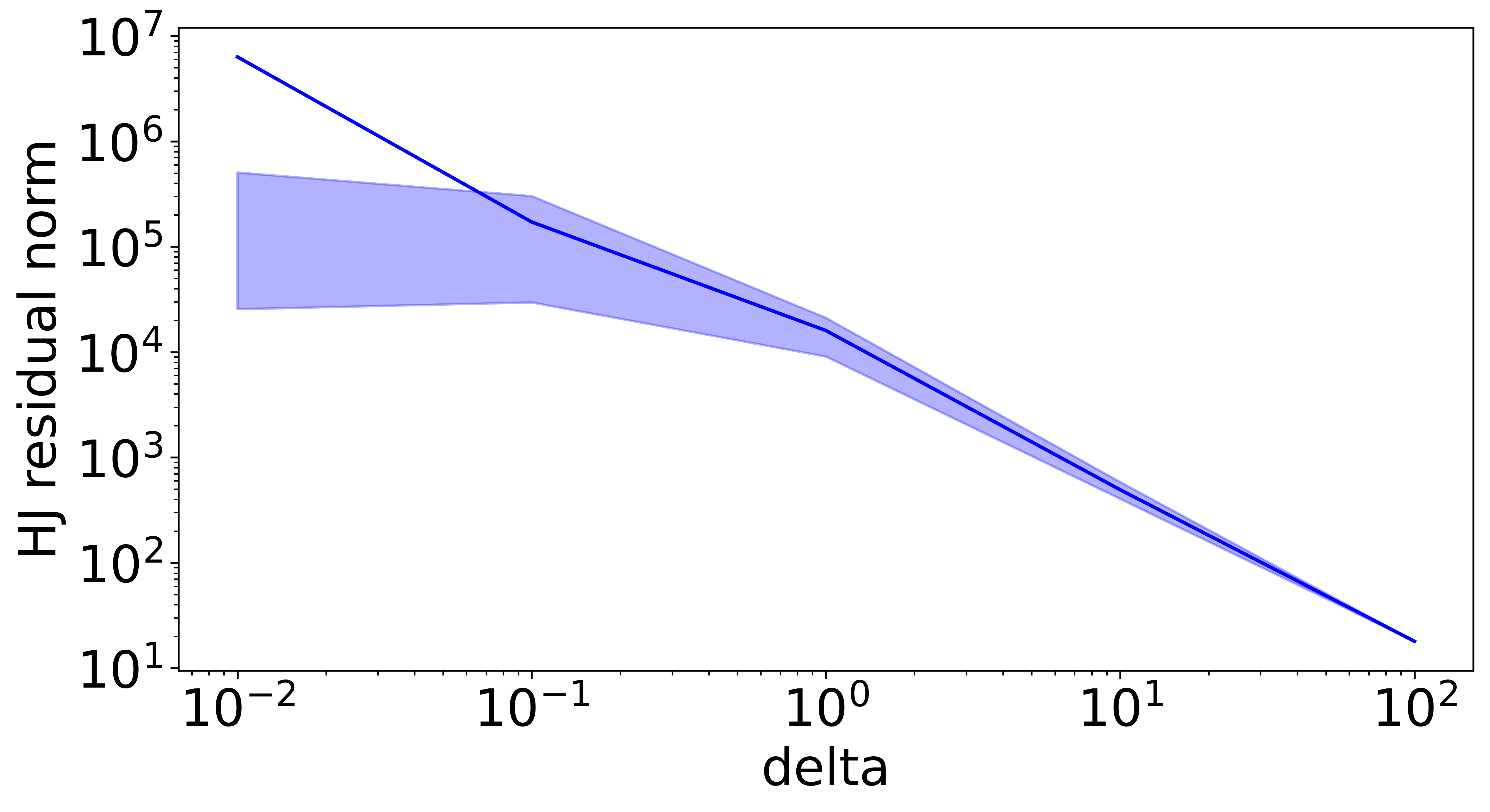
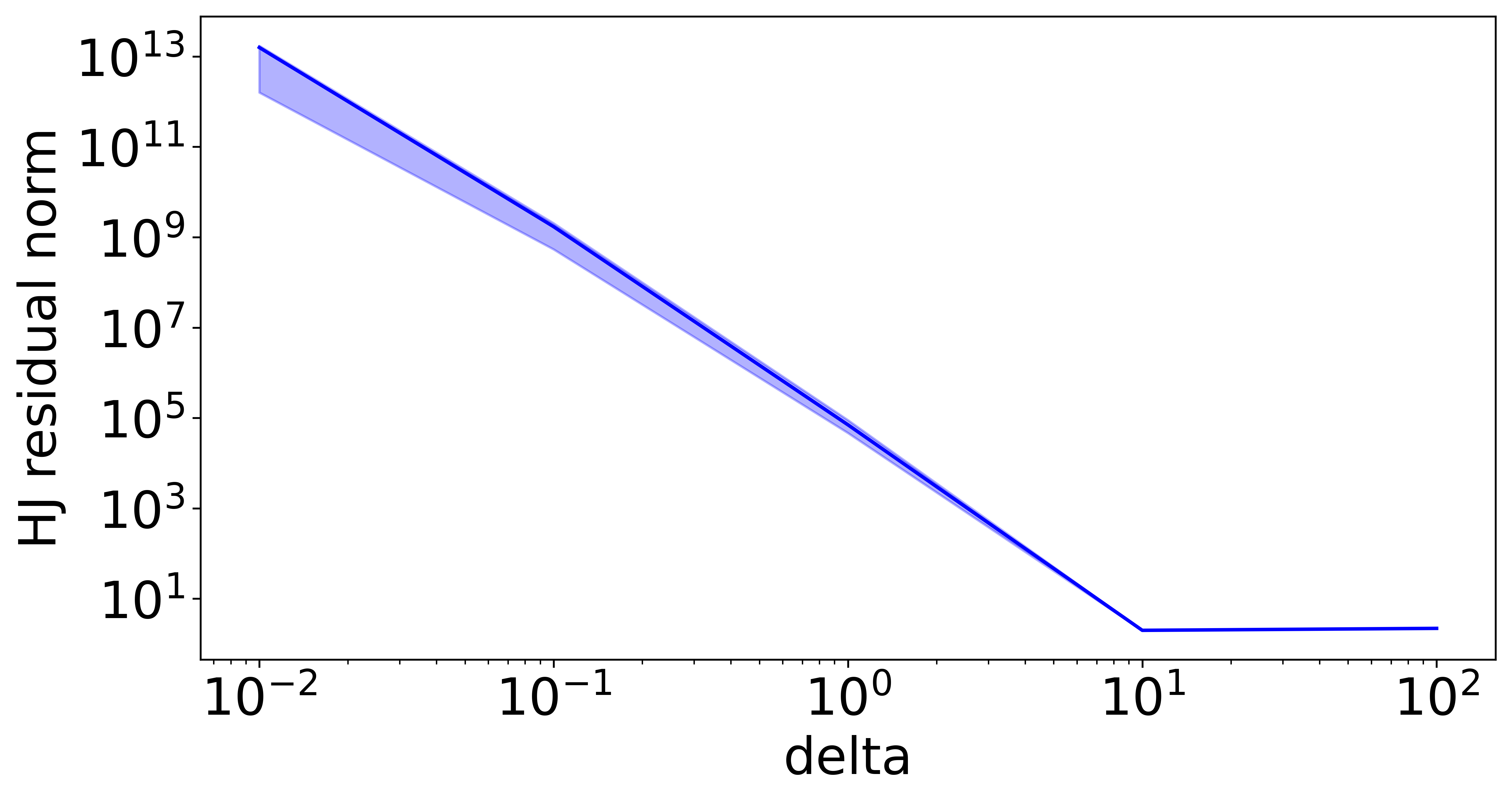
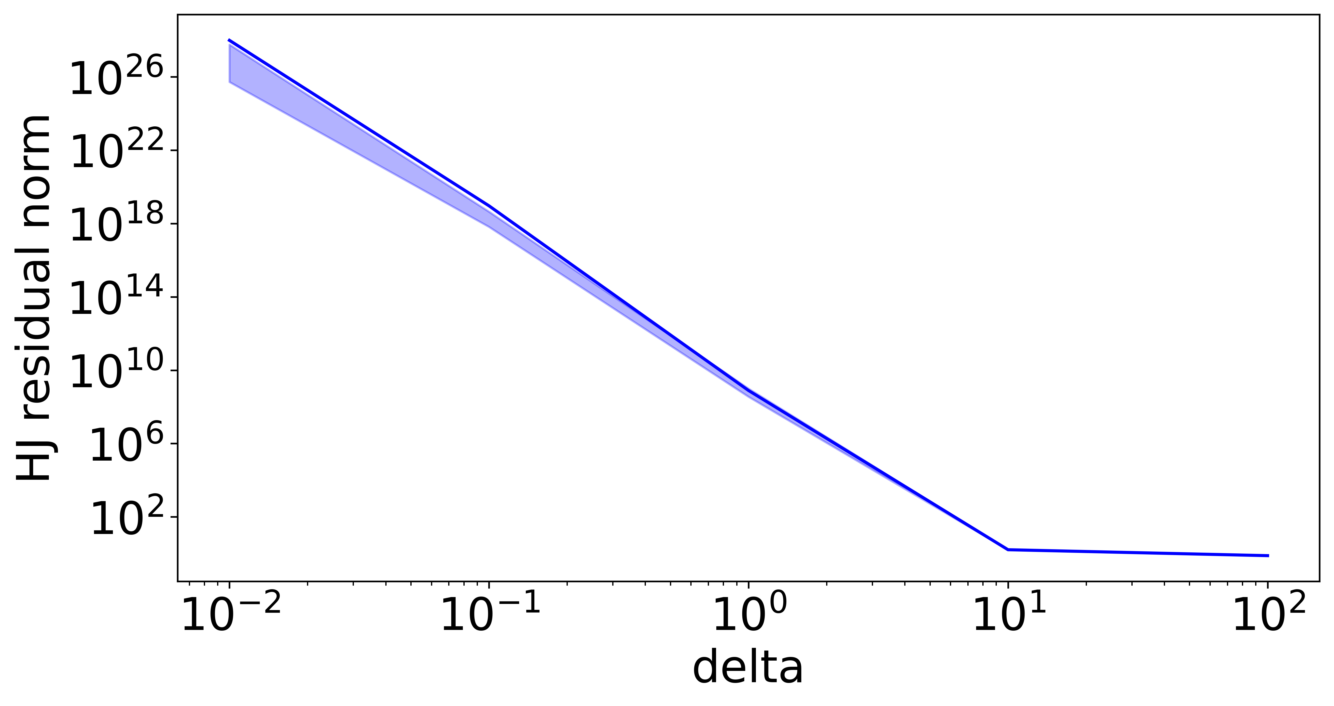
Figure 2: Median along with the 20th and 80th percentiles of HJ residuals in dimension 10 and Hamiltonians given by $H=\frac{1}{p}\|\cdot\|_{p}^{p}$, p = 1, 5, 10, from left to right. In these experiments, $10^{5}$ samples are used for the Monte Carlo approximation of the integrals in (6).

5 Deep Learning Methods

Deep learning methods have gained traction in solving high-dimensional HJ PDEs. Neural networks serve as flexible function approximators, leveraging optimization frameworks to approximate solutions. Without the need for discretization, these neural network methods are able to mitigate the curse of dimensionality. While deep learning methods for solving general PDEs [7] can be used here, we focus on works that are more specific to HJ PDEs.

5.1 Actor Critic Methods

In [76], the authors propose a numerical method for solving high-dimensional static HJ equations using an actor-critic framework combined with neural networks. The convergence of this method is analyzed in [77, 78]. The central equation they tackle takes the form:

$$\inf_{u\in U}\left[\frac{1}{2}\text{Tr}(\sigma\sigma^{\top}\text{Hess}(V))(x,u)+b(x,u)^{\top}\nabla V(x)+f(x,u)\right]-\gamma V(x)=0\quad\text{in }\Omega,$$

where $V$ is the value function, $u$ is the control, and $\gamma$ is the discount rate. Their key methodological contribution is a variance-reduced least squares temporal difference (VR-LSTD) method for policy evaluation. The critic step involves minimizing a loss functional $L_{1}(V)=\mathbb{E}[\text{TD}_{1}^{u}]^{2}$ with a quadratic loss term on boundary condition, where

$$\text{TD}_{1}^{u}=\int_{0}^{T}e^{-\gamma s}f(X_{s},u(X_{s}))ds-\int_{0}^{T}e^{-\gamma s}\nabla V(X_{s})^{\top}\sigma(X_{s},u(X_{s}))dW_{s}+e^{-\gamma T}V(X_{T})-V(X_{0}).$$

The actor step involves the following loss:

$$\mathbb{E}_{X_{0}\sim\mu,u}\left[\int_{0}^{T\wedge\tau}f(X_{s},u(X_{s}))e^{-\gamma s}\,\mathrm{d}s+V(X_{T\wedge\tau})e^{-\gamma(T\wedge\tau)}\right].$$

They show that this VR-LSTD method has better convergence properties than standard LSTD approaches.

To improve numerical accuracy near domain boundaries, they introduce an adaptive step size scheme when the sampled state is near the boundary. This scheme, combined with their neural network parameterization of both value and control functions, enables them to solve the equation up to 20 dimensions with relative errors typically around 1-5%. They demonstrate the effectiveness of their approach on several challenging problems including linear quadratic regulators, stochastic Van der Pol oscillators, and diffusive Eikonal equations, showing significant improvement over traditional numerical methods that struggle with the curse of dimensionality. For instance, they tested on the following diffusive Eikonal equation:

$$\left\{\begin{aligned} &\epsilon\Delta V(x)+\inf_{u\in B_{1}}\bigl{(}c(x)u^{\top}\nabla V(x)\bigr{)}+1=0~~~\text{in}~B_{R},\\ &V(x)=a_{3}-a_{2}~~~\text{on}~\partial B_{R},\end{aligned}\right.$$

where $c(x)$ is set to be $c(x)=\dfrac{3(d+1)a_{3}}{2da_{2}(2a_{2}-3a_{3}|x|)}>0$, and they choose $a_{2}=1.2$, $a_{3}=0.2$, and $R=1$. The numerical results are shown in Fig. 3. This methodology also applies to other formulations of control problems, such as finite-horizon settings, time-inhomogeneous systems, control without discounting, and problems without boundary conditions.

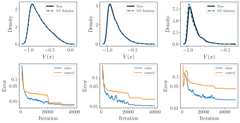
Figure 3: Top: density of the value of $V$ for the diffusive Eikonal equation with $d=5$ (left), $d=10$ (middle), and $d=20$ (right). Bottom: associated error curves in the training process with $d=5$ (left), $d=10$ (middle), and $d=20$ (right).

Another actor-critic approach [48] solves HJ PDEs with a viscosity term on the right-hand side. Here, a neural network method for solving high-dimensional stochastic mean-field games (MFGs) is proposed. Their framework tackles the coupled system of HJ PDEs and Fokker-Planck (FP) equations that characterize MFGs:

$$\begin{split}-\partial_{t}\phi-\nu\Delta\phi+H(x,\nabla\phi)=f(x,\rho),\quad\quad\partial_{t}\rho-\nu\Delta\rho-\text{div}(\rho\nabla_{p}H(x,\nabla\phi))=0,\end{split}$$ (7)

with initial condition $\rho(x,0)=\rho_{0}(x)$ and terminal condition $\phi(x,T)=g(x,\rho(\cdot,T))$. The authors reformulate this system as a convex-concave saddle-point problem, which they express as:

$$\begin{split}\inf_{\rho(x,0)=\rho_{0}(x)}\sup_{\phi}\int_{0}^{T}\int_{\Omega}(\partial_{t}\phi+\nu\Delta\phi-H(x,\nabla\phi))\rho(x,t)\,dx+F(\rho(\cdot,t))\,dt\\ +\int_{\Omega}\phi(x,0)\rho_{0}(x)\,dx-\int_{\Omega}\phi(x,T)\rho(x,T)\,dx+G(\rho(\cdot,T)),\end{split}$$

where the first variations of $F$ and $G$ are the functions $f$ and $g$ in (7). This variational structure allows them to parameterize $\rho$ and $\phi$ (the actor and the critic) with neural networks and train them in an alternating fashion, similar to generative adversarial networks (GANs) [35]. The resulting algorithm can approximate solutions to high-dimensional HJ PDEs, and in their experiments, HJ PDEs of dimensions up to 100 are solved efficiently [48, Section 5].

5.2 Neural Network Architectures Inspired by Representation Formulas

In this section, we review several works that propose neural network architectures inspired by representation formulas for HJ PDEs under different assumptions. These architectures, when assigned appropriate parameters based on their theoretical correspondence, inherit rigorous guarantees from HJ theory—eliminating the need for a traditional training process.

In [25, 27, 23], different neural network architectures are designed based on the representation formulas of solution to certain classes of HJ PDEs. In [25], inspired by the Hopf formula (4), a shallow neural network with a max activation function is proposed to solve HJ PDEs. Specifically, the formula for the neural network is

$$\phi(x,t;\{(p_{i},\theta_{i},\gamma_{i})\}_{i=1}^{m})=\max_{i=1,\dots,m}\left\{\langle p_{i},x\rangle-t\theta_{i}-\gamma_{i}\right\},$$

where $\{(p_{i},\theta_{i},\gamma_{i})\}_{i=1}^{m}$ denotes the parameters in the neural network. Moreover, it is proven that, under certain technical assumptions, if there exists a convex interpolation for $(p_{i},\gamma_{i})$ and the points $p_{1},\dots,p_{m}$ are distinct, then the function represented by the neural network is the viscosity solution to the HJ PDE with the initial condition $J$ given by

$$J(x)=\max_{i=1,\dots,m}\left\{\langle p_{i},x\rangle-\gamma_{i}\right\},$$

and the Hamiltonian $H$ defined as

$$H({p})=\begin{dcases}\inf\limits_{\alpha\in\mathcal{A}({p})}\left\{\sum_{i=1}^{m}\alpha_{i}\theta_{i}\right\},&\text{if }{p}\in\operatorname{dom}J^{*},\\ +\infty,&\text{otherwise}.\end{dcases}$$ (8)

Here, the set $\mathcal{A}({p})$ is characterized as

$$\mathcal{A}({p})=\operatorname*{arg\,min}_{\begin{subarray}{c}\alpha_{1},\dots,\alpha_{m}\geq 0\\ \sum_{i=1}^{m}\alpha_{i}=1\\ \sum_{i=1}^{m}\alpha_{i}{p}_{i}={p}\end{subarray}}\left\{\sum_{i=1}^{m}\alpha_{i}\gamma_{i}\right\}.$$

Moreover, for a fixed set of parameters $\{(p_{i},\theta_{i},\gamma_{i})\}_{i=1}^{m}$, the neural network representation is capable of solving multiple HJ PDEs. Specifically, it solves the HJ PDE with a spatially and temporally independent Hamiltonian $\tilde{H}$ if and only if the conditions $\tilde{H}(p_{i})=H(p_{i})\,\forall i=1,\dots,m$ and $\tilde{H}(p)\geq H(p)\,\forall p\in\operatorname{dom}J^{*}$ are both satisfied. Here, the function $H$ is the Hamiltonian defined in (8).

In [27], based on the Lax-Oleinik formula (3), the authors propose two neural network architectures that solve two classes of HJ PDEs, respectively. The first architecture is designed as

$$\phi({x},t;\{(u_{i},a_{i})\}_{i=1}^{m})=\min_{i=1,\dots,m}\left\{tL\left(\frac{x-u_{i}}{t}\right)+a_{i}\right\}.$$

This is a two-layer neural network employing an activation function $L$ and a minimum operator. Under certain assumptions, this architecture computes the viscosity solution of an HJ PDE whose Hamiltonian is given by the convex conjugate $L^{*}$, independent of the spatial and temporal variables $(x,t)$. The corresponding initial condition is expressed as the minimum of shifts of the asymptotic function associated with $L$. Similarly, the second architecture utilizes an activation function $J$ combined with a minimum operator. Under suitable conditions, this network solves the HJ PDE characterized by a piecewise affine Hamiltonian and a concave initial condition given by $J$.

In [23], the authors propose a ResNet-type deep neural network based on the linear-quadratic regulator framework and min-plus algebra to solve HJ PDEs. These PDEs have quadratic Hamiltonians $H(p,x,t)$ with respect to $(p,x)$, whose coefficients depend on time $t$, and initial conditions expressed as the minimum of several quadratic functions. Additionally, the authors design a neural network architecture to compute the optimal control and corresponding optimal trajectories associated with these control problems. The numerical results for HJ PDEs exhibiting Newtonian dynamics, originally presented in [23], are reproduced in Figs. 4 and 5. Specifically, the simulations consider the dimension setting $n=2m=16$, with the Lagrangian $L$ defined by

$$L(u,x,t)=\frac{1}{2}\left\|x-5\sin t\begin{pmatrix}\mathbf{1}\\ \mathbf{0}\end{pmatrix}+5\cos t\begin{pmatrix}\mathbf{0}\\ \mathbf{1}\end{pmatrix}\right\|^{2}+\frac{1}{2000}\|u\|^{2},$$ (9)

and the source term $f$ given by

$$f(u,x,t)=\begin{pmatrix}O&I\\ O&O\end{pmatrix}x+\begin{pmatrix}O\\ I\end{pmatrix}u,$$ (10)

for $u\in\mathbb{R}^{m}$, $x\in\mathbb{R}^{n}$, and $t\in[0,T]$. Here, $\mathbf{1}$ and $\mathbf{0}$ represent the one and zero constant vectors in $\mathbb{R}^{m}$, while $O$ and $I$ denote the $m\times m$ zero and identity matrices, respectively. The terminal cost function $J\colon\mathbb{R}^{n}\to\mathbb{R}$ is defined as

$$J(x)=\min\left\{\frac{1}{320}\left((x_{1}+2)^{2}+\sum_{i=2}^{n}x_{i}^{2}\right),\frac{1}{320}\left((x_{1}-2)^{2}+\sum_{i=2}^{n}x_{i}^{2}\right)\right\},$$ (11)

for $x=(x_{1},x_{2},\dots,x_{n})\in\mathbb{R}^{n}$. Fig. 4 shows two-dimensional slices of the computed HJ PDE solutions at different times. Furthermore, Fig. 5 displays the optimal trajectories corresponding to terminal times $T=1$, $T=5$, and $T=10$ from various initial positions $x_{0}=(x,\mathbf{0})\in\mathbb{R}^{16}$ (where $\mathbf{0}\in\mathbb{R}^{15}$ is the zero vector).

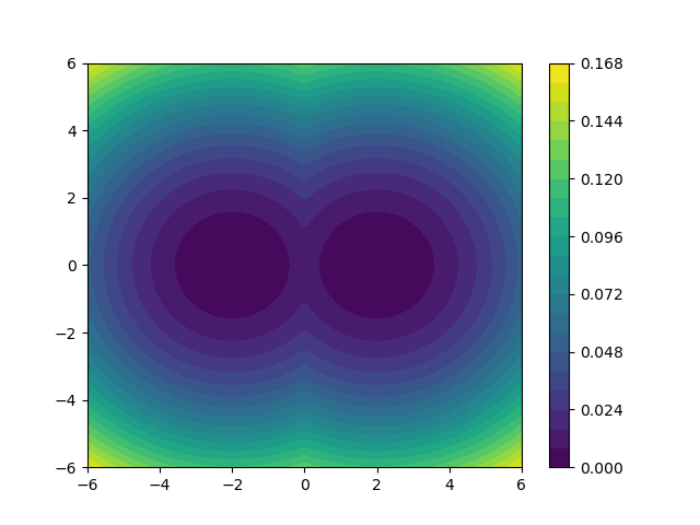
(a) $t=1$

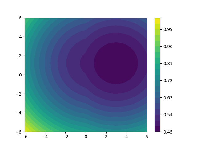
(b) $t=0.995$

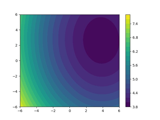
(c) $t=0.95$

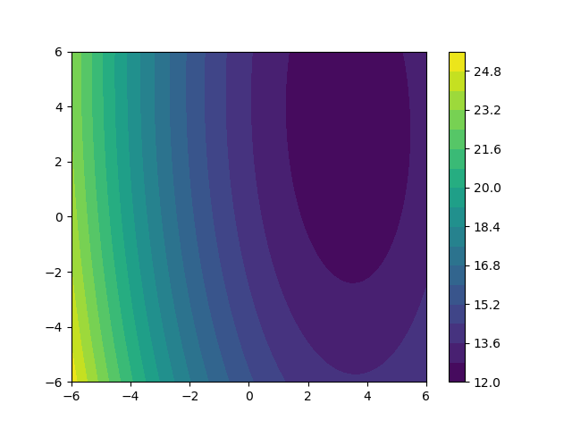
(d) $t=0.75$

Figure 4: Visualization of the viscosity solution to the 16-dimensional HJ PDE with initial condition (11), corresponding to the running cost $L$ defined by (9), dynamics $f$ defined by (10), and terminal time $T=1$. Two-dimensional slices at times $t=1$ (terminal cost), $t=0.995$, $t=0.95$, and $t=0.75$ are displayed in subfigures (a), (b), (c), and (d), respectively. Each subfigure shows solution values (indicated by color) at points of the form $(x_{1},\mathbf{0},x_{2},\mathbf{0})\in\mathbb{R}^{16}$, where $x_{1}$ and $x_{2}$ correspond to the horizontal and vertical axes, and $\mathbf{0}$ denotes a 7-dimensional zero vector.

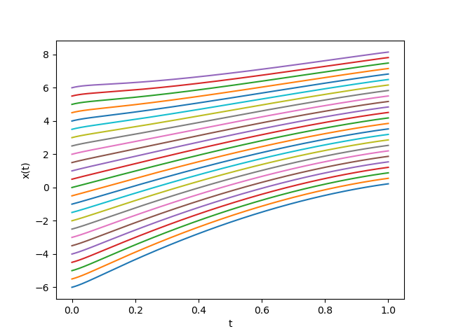
(a) $x_{1}^{*}$, $T=1$

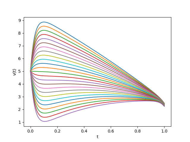
(b) $x_{9}^{*}$, $T=1$

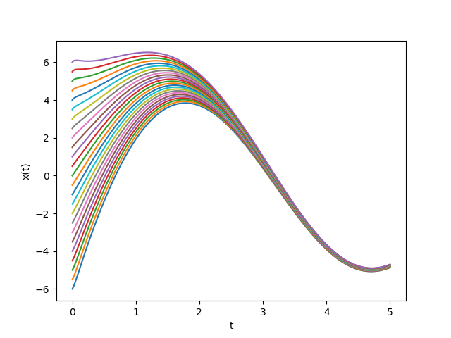
(c) $x_{1}^{*}$, $T=5$

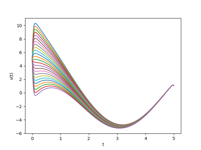
(d) $x_{9}^{*}$, $T=5$

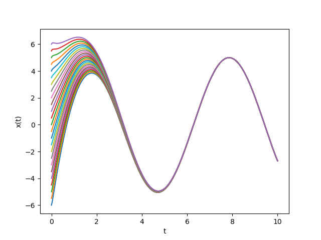
(e) $x_{1}^{*}$, $T=10$

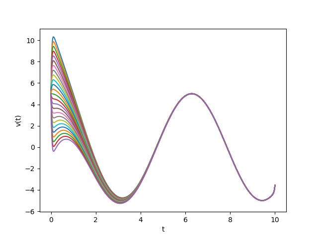
(f) $x_{9}^{*}$, $T=10$

Figure 5: Visualization of optimal trajectories $x^{*}$ for the 16-dimensional optimal control problem with running cost $L$ given by (9), dynamics given by (10), terminal cost (11), and terminal times $T=1,\,5,\,10$. Panels (a), (c), and (e) display the evolution of the first component $x_{1}^{*}$ of the optimal trajectories, while panels (b), (d), and (f) display the corresponding evolution of the ninth component $x_{9}^{*}$. In each panel, different curves represent trajectories originating from different initial conditions $x_{0}=(x,\mathbf{0})\in\mathbb{R}^{16}$, where $\mathbf{0}$ is the zero vector in $\mathbb{R}^{15}$.

6 Saddle Point Methods

In this section, we review recent numerical methods [52, 53] for solving HJ PDEs based on saddle-point formulations. These approaches exploit connections between HJ PDEs and problems in optimal transport and mean-field games by reformulating the PDEs as components of certain saddle-point problems. Upon spatial discretization, the resulting optimization problems can be efficiently solved using primal-dual algorithms, such as the Primal-Dual Hybrid Gradient (PDHG) algorithm [10]. Specifically, we consider the HJ PDE (1) defined on a rectangular spatial domain $\Omega=\prod_{i=1}^{n}[a_{i},b_{i}]$ with periodic boundary conditions.

In [52], the solution $\phi$ is represented as a part of the saddle point to the following problem

$$\min_{\begin{subarray}{c}\phi\\ \phi(x,0)=J(x)\end{subarray}}\max_{\rho}\int_{0}^{T}\int_{\Omega}\rho(x,t)\left(\frac{\partial\phi(x,t)}{\partial t}+\max_{v\in\mathbb{R}^{n}}\left\{\langle v,\nabla_{x}\phi(x,t)\rangle-H^{*}\left(v,x,t\right)\right\}\right)dxdt-c\int_{\Omega}\phi(x,T)dx,$$

where $c>0$ is a hyperparameter, and $H^{*}(\cdot,x,t)$ is the Fenchel-Legendre transform of $H(\cdot,x,t)$. If we further assume the function $\rho$ in the saddle point is non-negative, then the problem becomes

$$\begin{split}\min_{\begin{subarray}{c}\phi\\ \phi(x,0)=J(x)\end{subarray}}\max_{\begin{subarray}{c}\rho,v\\ \rho\geq 0\end{subarray}}\int_{0}^{T}\int_{\Omega}\rho(x,t)\left(\frac{\partial\phi(x,t)}{\partial t}+\langle v(x,t),\nabla_{x}\phi(x,t)\rangle-H^{*}\left(v(x,t),x,t\right)\right)dxdt-c\int_{\Omega}\phi(x,T)dx,\end{split}$$

which is in the form of simple mean-field games. After applying a first-order monotone scheme with a numerical Hamiltonian $\hat{H}\colon(\mathbb{R}^{n})^{2n}\times\mathbb{R}^{n}\times[0,T]\to\mathbb{R}$, the corresponding discretized saddle point formulation can be solved using PDHG. In [52], the 1-dimensional saddle point formula is discretized as

$$\min_{\begin{subarray}{c}\phi_{i,k}\forall i,k\\ \phi_{i,1}=J(x_{i})\end{subarray}}\max_{\begin{subarray}{c}\rho_{i,k},v^{+}_{i,k},v^{-}_{i,k}\forall i,k\\ \rho_{i,k}\geq 0\end{subarray}}\sum_{i=1}^{n_{x}}\sum_{k=1}^{n_{t}-1}\rho_{i,k}\Bigg{(}(D_{t}^{-}\phi)_{i,k+1}+v^{+}_{i,k}(D_{x}^{+}\phi)_{i,k+1}+v^{-}_{i,k}(D_{x}^{-}\phi)_{i,k+1}$$ (12)

$$-\hat{H}^{*}\left(v^{+}_{i,k},v^{-}_{i,k},x_{i},t_{k+1}\right)\Bigg{)}-\frac{c}{\Delta t}\sum_{i=1}^{n_{x}}\phi_{i,n_{t}}.$$

Here, $x_{1},\dots,x_{n_{x}}$ denote the discretization points of the spatial domain $[a,b]$, and $t_{1},\dots,t_{n_{t}}$ represent the discretization points of the temporal domain $[0,T]$. The values $\phi_{i,k},v^{+}_{i,k},v^{-}_{i,k},\rho_{i,k}$ correspond to the function values at the grid point $(x_{i},t_{k})$. For finite difference approximations, we use $D_{t}^{-}$, $D_{x}^{+}$, and $D_{x}^{-}$ to denote the backward Euler temporal difference, right spatial difference, and left spatial difference, respectively. Specifically, these are defined as $(D_{t}^{-}\phi)_{i,k}=\frac{\phi_{i,k}-\phi_{i,k-1}}{\Delta t}$, $(D_{x}^{+}\phi)_{i,k}=\frac{\phi_{i+1,k}-\phi_{i,k}}{\Delta x}$, and $(D_{x}^{-}\phi)_{i,k}=\frac{\phi_{i,k}-\phi_{i-1,k}}{\Delta x}$. According to the theory of first-order monotone schemes, the numerical Hamiltonian $\hat{H}$ must satisfy two key properties:

• Consistency: $\hat{H}(p,p,x,t)=H(p,x,t)$.

• Monotonicity: $\hat{H}$ must be non-increasing with respect to $p^{+}$ and non-decreasing with respect to $p^{-}$.

We denote the Fenchel-Legendre transform of $\hat{H}(\cdot,\cdot,x,t)$ by $\hat{H}^{*}(\cdot,\cdot,x,t)$. The PDHG method is then applied to compute the saddle point of problem (12), where the first part of the solution provides the numerical approximation to the corresponding HJ PDE. Fig. 6 presents a numerical result from [52], which solves the HJ PDE with the Hamiltonian $H(p,x)=\|p\|+3\exp(-4\|x-1\|^{2})+1$ and the initial condition $J(x)=\sum_{i=1}^{n}\sin(\pi x_{i})$.

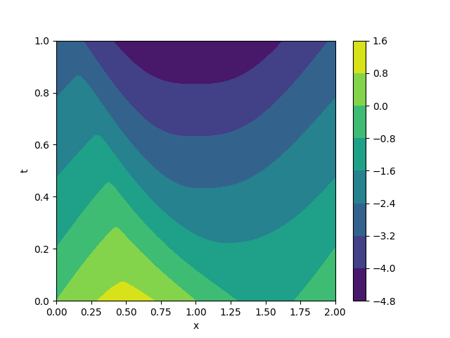
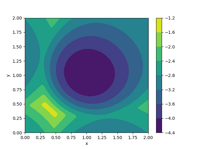
Figure 6: Contour plots illustrating the solution of the HJ PDE with Hamiltonian $H(p,x)=\|p\|+3\exp(-4\|x-1\|^{2})+1$ and initial condition $J(x)=\sum_{i=1}^{n}\sin(\pi x_{i})$. The left panel shows the solution for the one-dimensional case, while the right panel presents the level sets at $t=0.75$ for the two-dimensional case.

In [53], the authors proposed solving the HJ PDE and the corresponding optimal control problem using the following saddle point formula

where $f_{x,t}(\alpha)$ and $L_{x,t}(\alpha)$ denote $f(\alpha,x,T-t)$ and $L(\alpha,x,T-t)$, and $c$ is a positive hyperparameter. A one-dimensional discretization gives

$$\begin{split}\min_{\begin{subarray}{c}\phi\\ \phi_{i,1}=J(x_{i})\end{subarray}}\max_{\rho\geq 0,\alpha}\sum_{k=2}^{n_{t}}\sum_{i=1}^{n_{x}}\rho_{i,k}\Bigg{(}(D_{t}^{-}\phi)_{i,k}-f_{i,k}(\alpha_{1,i,k})_{+}(D_{x}^{+}\phi)_{i,k}-f_{i,k}(\alpha_{2,i,k})_{-}(D_{x}^{-}\phi)_{i,k}\\ -\hat{L}_{i,k}\left(\alpha_{1,i,k},\alpha_{2,i,k}\right)\Bigg{)}-\frac{c}{\Delta t}\sum_{i=1}^{n_{x}}\phi_{i,n_{t}}.\end{split}$$

Here, $\hat{L}_{i,k}$ represents the numerical Lagrangian at $(x_{i},t_{k})$, and other notations follow the conventions introduced earlier in [52]. The resulting saddle-point problem is then solved using the PDHG method. Notably, this work can be seen as a generalization of [52] for cases where $f(\alpha,x,t)\neq\alpha$. When considering more general dynamics, the saddle-point formulation in (13) not only yields the solution $\phi$ to the HJ PDE but also provides the optimal control function $\alpha$ in a feedback form, making it particularly well-suited for optimal control problems.

7 Conclusion

This review explores several recent approaches for numerically solving Hamilton-Jacobi partial differential equations, ranging from classical grid-based methods to emerging deep learning techniques. Each approach offers distinct advantages: grid-based methods provide robust frameworks for handling complex geometries, representation formulas capture underlying mathematical structures, Laplace approximations provide sampling based schemes, deep learning methods show promise in handling complex boundary conditions and high-dimensional settings, and saddle point methods make connections to mean-field games and have potentials to solve more complicated problems. While we highlight these recent developments, this review is by no means comprehensive. Notable approaches like optimal control algorithms [61, 54, 60, 62], optimal transport [56, 70, 71], and mean-field games/control [65, 19, 8, 9, 69, 4] offer alternative paths to solving HJ PDEs. The field of numerical methods for Hamilton-Jacobi equations continues to evolve rapidly, with substantial work existing beyond what we have covered. New hybrid approaches emerge regularly, combining strengths from different methodological frameworks. The ongoing integration of ideas from different methodological approaches, combined with advances in computational capabilities, suggests a promising future for the numerical solution of Hamilton-Jacobi PDEs.

References

- [1] R. Abedian. WENO schemes with adaptive order for Hamilton–Jacobi equations. International Journal of Modern Physics C, 34(06):2350081, 2023.
- [2] R. Abedian and M. Dehghan. RBF-ENO/WENO schemes with Lax–Wendroff type time discretizations for Hamilton–Jacobi equations. Numerical Methods for Partial Differential Equations, 37(1):594–613, 2021.
- [3] R. Abgrall. Numerical discretization of the first-order Hamilton-Jacobi equation on triangular meshes. Communications on pure and applied mathematics, 49(12):1339–1373, 1996.
- [4] S. Agrawal, W. Lee, S. Wu Fung, and L. Nurbekyan. Random features for high-dimensional nonlocal mean-field games. Journal of Computational Physics, 459:111136, 2022.
- [5] M. Bardi, I. C. Dolcetta, et al. Optimal control and viscosity solutions of Hamilton-Jacobi-Bellman equations, volume 12. Springer, 1997.
- [6] M. Bardi and S. Faggian. Hopf-type estimates and formulas for nonconvex nonconcave Hamilton–Jacobi equations. SIAM Journal on Mathematical Analysis, 29(5):1067–1086, 1998.
- [7] C. Beck, M. Hutzenthaler, A. Jentzen, and B. Kuckuck. An overview on deep learning-based approximation methods for partial differential equations. Discrete & Continuous Dynamical Systems-Series B, 28(6), 2023.
- [8] R. Carmona and M. Laurière. Convergence analysis of machine learning algorithms for the numerical solution of mean field control and games I: The ergodic case. SIAM Journal on Numerical Analysis, 59(3):1455–1485, 2021.
- [9] R. Carmona and M. Laurière. Convergence analysis of machine learning algorithms for the numerical solution of mean field control and games: II—the finite horizon case. The Annals of Applied Probability, 32(6):4065–4105, 2022.
- [10] A. Chambolle and T. Pock. A first-order primal-dual algorithm for convex problems with applications to imaging. Journal of mathematical imaging and vision, 40:120–145, 2011.
- [11] P. Chen, J. Darbon, and T. Meng. Hopf-type representation formulas and efficient algorithms for certain high-dimensional optimal control problems. Computers & Mathematics with Applications, 161:90–120, 2024.
- [12] P. Chen, J. Darbon, and T. Meng. Lax-Oleinik-type formulas and efficient algorithms for certain high-dimensional optimal control problems. Communications on Applied Mathematics and Computation, pages 1–44, 2024.
- [13] Y. Cheng and C.-W. Shu. A discontinuous Galerkin finite element method for directly solving the Hamilton–Jacobi equations. Journal of Computational Physics, 223(1):398–415, 2007.
- [14] Y. Cheng and Z. Wang. A new discontinuous Galerkin finite element method for directly solving the Hamilton–Jacobi equations. Journal of Computational Physics, 268:134–153, 2014.
- [15] Y. T. Chow, J. Darbon, S. Osher, and W. Yin. Algorithm for overcoming the curse of dimensionality for time-dependent non-convex Hamilton–Jacobi equations arising from optimal control and differential games problems. Journal of Scientific Computing, 73:617–643, 2017.
- [16] Y. T. Chow, J. Darbon, S. Osher, and W. Yin. Algorithm for overcoming the curse of dimensionality for certain non-convex Hamilton–Jacobi equations, projections and differential games. Ann. Math. Sci. Appl, 3(2):369–403, 2018.
- [17] Y. T. Chow, J. Darbon, S. Osher, and W. Yin. Algorithm for overcoming the curse of dimensionality for state-dependent Hamilton-Jacobi equations. Journal of Computational Physics, 387:376–409, 2019.
- [18] Y. T. Chow, W. Li, S. Osher, and W. Yin. Algorithm for Hamilton–Jacobi equations in density space via a generalized Hopf formula. Journal of Scientific Computing, 80:1195–1239, 2019.
- [19] Y. T. Chow, S. Wu Fung, S. Liu, L. Nurbekyan, and S. Osher. A numerical algorithm for inverse problem from partial boundary measurement arising from mean field game problem. Inverse Problems, 39(1):014001, 2022.
- [20] B. Cockburn and C.-W. Shu. The Runge-Kutta local projection-discontinuous-Galerkin finite element method for scalar conservation laws. ESAIM: Mathematical Modelling and Numerical Analysis, 25(3):337–361, 1991.
- [21] M. Crandal and P. Lions. Two approximations of solutions of Hamilton–Jacobi equations. Math. Comp, 43(167):1–19, 1984.
- [22] M. G. Crandall and P.-L. Lions. Viscosity solutions of Hamilton-Jacobi equations. Transactions of the American mathematical society, 277(1):1–42, 1983.
- [23] J. Darbon, P. M. Dower, and T. Meng. Neural network architectures using min-plus algebra for solving certain high-dimensional optimal control problems and Hamilton–Jacobi PDEs. Mathematics of Control, Signals, and Systems, 35(1):1–44, 2023.
- [24] J. Darbon and G. P. Langlois. On Bayesian posterior mean estimators in imaging sciences and Hamilton–Jacobi partial differential equations. Journal of Mathematical Imaging and Vision, 63(7):821–854, 2021.
- [25] J. Darbon, G. P. Langlois, and T. Meng. Overcoming the curse of dimensionality for some Hamilton–Jacobi partial differential equations via neural network architectures. Research in the Mathematical Sciences, 7(3):20, 2020.
- [26] J. Darbon, G. P. Langlois, and T. Meng. Connecting Hamilton-Jacobi partial differential equations with maximum a posteriori and posterior mean estimators for some non-convex priors. Handbook of Mathematical Models and Algorithms in Computer Vision and Imaging: Mathematical Imaging and Vision, pages 1–25, 2021.
- [27] J. Darbon and T. Meng. On some neural network architectures that can represent viscosity solutions of certain high dimensional Hamilton–Jacobi partial differential equations. Journal of Computational Physics, 425:109907, 2021.
- [28] J. Darbon and S. Osher. Algorithms for overcoming the curse of dimensionality for certain Hamilton–Jacobi equations arising in control theory and elsewhere. Research in the Mathematical Sciences, 3(1):19, 2016.
- [29] P. M. Dower, W. M. McEneaney, and H. Zhang. Max-plus fundamental solution semigroups for optimal control problems. In 2015 Proceedings of the Conference on Control and its Applications, pages 368–375. SIAM, 2015.
- [30] L. C. Evans. Partial differential equations, volume 19. American Mathematical Society, 2022.
- [31] M. Falcone and R. Ferretti. Numerical methods for Hamilton–Jacobi type equations. In Handbook of Numerical Analysis, volume 17, pages 603–626. Elsevier, 2016.
- [32] W. H. Fleming and W. M. McEneaney. A max-plus-based algorithm for a Hamilton–Jacobi–Bellman equation of nonlinear filtering. SIAM Journal on Control and Optimization, 38(3):683–710, 2000.
- [33] W. H. Fleming and H. M. Soner. Controlled Markov processes and viscosity solutions, volume 25. Springer Science & Business Media, 2006.
- [34] S. Gaubert, W. McEneaney, and Z. Qu. Curse of dimensionality reduction in max-plus based approximation methods: Theoretical estimates and improved pruning algorithms. In 2011 50th IEEE Conference on Decision and Control and European Control Conference, pages 1054–1061. IEEE, 2011.
- [35] I. Goodfellow, J. Pouget-Abadie, M. Mirza, B. Xu, D. Warde-Farley, S. Ozair, A. Courville, and Y. Bengio. Generative adversarial networks. Communications of the ACM, 63(11):139–144, 2020.
- [36] W. Guo, J. Huang, Z. Tao, and Y. Cheng. An adaptive sparse grid local discontinuous Galerkin method for Hamilton-Jacobi equations in high dimensions. Journal of Computational Physics, 436:110294, 2021.
- [37] H. Heaton, S. Wu Fung, and S. Osher. Global solutions to nonconvex problems by evolution of Hamilton-Jacobi PDEs. Communications on Applied Mathematics and Computation, 6(2):790–810, 2024.
- [38] C. Hu and C.-W. Shu. A discontinuous Galerkin finite element method for Hamilton–Jacobi equations. SIAM Journal on Scientific computing, 21(2):666–690, 1999.
- [39] J. Kaipio and E. Somersalo. Statistical and computational inverse problems, volume 160. Springer Science & Business Media, 2006.
- [40] C. H. Kim, Y. Ha, H. Yang, and J. Yoon. A third-order WENO scheme based on exponential polynomials for Hamilton-Jacobi equations. Applied Numerical Mathematics, 165:167–183, 2021.
- [41] M. R. Kirchner, G. Hewer, J. Darbon, and S. Osher. A primal-dual method for optimal control and trajectory generation in high-dimensional systems. In 2018 IEEE Conference on Control Technology and Applications (CCTA), pages 1583–1590. IEEE, 2018.
- [42] M. R. Kirchner, R. Mar, G. Hewer, J. Darbon, S. Osher, and Y. T. Chow. Time-optimal collaborative guidance using the generalized Hopf formula. IEEE Control Systems Letters, 2(2):201–206, 2017.
- [43] C. Klingenberg, G. Schnücke, and Y. Xia. An arbitrary Lagrangian–Eulerian local discontinuous Galerkin method for Hamilton–Jacobi equations. Journal of Scientific Computing, 73:906–942, 2017.
- [44] P. S. Laplace. Mémoire sur la probabilité de causes par les évenements. Mémoire de l’académie royale des sciences, 1774.
- [45] B. Lee, J. Darbon, S. Osher, and M. Kang. Revisiting the redistancing problem using the Hopf–Lax formula. Journal of Computational Physics, 330:268–281, 2017.
- [46] F. Li and C.-W. Shu. Reinterpretation and simplified implementation of a discontinuous Galerkin method for Hamilton–Jacobi equations. Applied Mathematics Letters, 18(11):1204–1209, 2005.
- [47] F. Li and S. Yakovlev. A central discontinuous Galerkin method for Hamilton-Jacobi equations. Journal of Scientific Computing, 45(1):404–428, 2010.
- [48] A. T. Lin, S. Wu Fung, W. Li, L. Nurbekyan, and S. J. Osher. Alternating the population and control neural networks to solve high-dimensional stochastic mean-field games. Proceedings of the National Academy of Sciences, 118(31):e2024713118, 2021.
- [49] H. Liu and M. Pollack. Alternating evolution discontinuous Galerkin methods for Hamilton–Jacobi equations. Journal of Computational Physics, 258:31–46, 2014.
- [50] X.-D. Liu, S. Osher, and T. Chan. Weighted essentially non-oscillatory schemes. Journal of computational physics, 115(1):200–212, 1994.
- [51] W. M. McEneaney. Max-plus methods for nonlinear control and estimation. Springer Science & Business Media, 2006.
- [52] T. Meng, W. Hao, S. Liu, S. J. Osher, and W. Li. Primal-dual hybrid gradient algorithms for computing time-implicit Hamilton-Jacobi equations. arXiv preprint arXiv:2310.01605, 2023.
- [53] T. Meng, S. Liu, W. Li, and S. Osher. A primal-dual hybrid gradient method for solving optimal control problems and the corresponding Hamilton-Jacobi PDEs. arXiv preprint arXiv:2403.02468, 2024.
- [54] D. Onken, L. Nurbekyan, X. Li, S. Wu Fung, S. Osher, and L. Ruthotto. A neural network approach applied to multi-agent optimal control. In 2021 European Control Conference (ECC), pages 1036–1041. IEEE, 2021.
- [55] D. Onken, L. Nurbekyan, X. Li, S. Wu Fung, S. Osher, and L. Ruthotto. A neural network approach for high-dimensional optimal control applied to multiagent path finding. IEEE Transactions on Control Systems Technology, 31(1):235–251, 2022.
- [56] D. Onken, S. Wu Fung, X. Li, and L. Ruthotto. OT-flow: Fast and accurate continuous normalizing flows via optimal transport. In Proceedings of the AAAI Conference on Artificial Intelligence, volume 35, pages 9223–9232, 2021.
- [57] S. Osher, H. Heaton, and S. Wu Fung. A Hamilton–Jacobi-based proximal operator. Proceedings of the National Academy of Sciences, 120(14):e2220469120, 2023.
- [58] S. Osher and J. A. Sethian. Fronts propagating with curvature-dependent speed: Algorithms based on Hamilton-Jacobi formulations. Journal of computational physics, 79(1):12–49, 1988.
- [59] S. Osher and C.-W. Shu. High-order essentially nonoscillatory schemes for Hamilton–Jacobi equations. SIAM Journal on numerical analysis, 28(4):907–922, 1991.
- [60] C. Parkinson, D. Arnold, A. L. Bertozzi, Y. T. Chow, and S. Osher. Optimal human navigation in steep terrain: a Hamilton-Jacobi-Bellman approach. arXiv preprint arXiv:1805.04973, 2018.
- [61] C. Parkinson, A. L. Bertozzi, and S. J. Osher. A Hamilton-Jacobi formulation for time-optimal paths of rectangular nonholonomic vehicles. In 2020 59th IEEE Conference on Decision and Control (CDC), pages 4073–4078. IEEE, 2020.
- [62] C. Parkinson and M. Ceccia. Time-optimal paths for simple cars with moving obstacles in the Hamilton-Jacobi formulation. In 2022 American Control Conference (ACC), pages 2944–2949. IEEE, 2022.
- [63] D. Peng, B. Merriman, S. Osher, H. Zhao, and M. Kang. A PDE-based fast local level set method. Journal of computational physics, 155(2):410–438, 1999.
- [64] J. Qiu and C.-W. Shu. Hermite WENO schemes for Hamilton–Jacobi equations. Journal of Computational Physics, 204(1):82–99, 2005.
- [65] L. Ruthotto, S. J. Osher, W. Li, L. Nurbekyan, and S. Wu Fung. A machine learning framework for solving high-dimensional mean field game and mean field control problems. Proceedings of the National Academy of Sciences, 117(17):9183–9193, 2020.
- [66] C.-W. Shu. High order numerical methods for time dependent Hamilton-Jacobi equations. In Mathematics and computation in imaging science and information processing, pages 47–91. World Scientific, 2007.
- [67] C.-W. Shu and S. Osher. Efficient implementation of essentially non-oscillatory shock-capturing schemes. Journal of computational physics, 77(2):439–471, 1988.
- [68] R. J. Tibshirani, S. Wu Fung, H. Heaton, and S. Osher. Laplace meets Moreau: Smooth approximation to infimal convolutions using Laplace’s method. arXiv preprint arXiv:2406.02003, 2024.
- [69] A. Vidal, S. Wu Fung, S. Osher, L. Tenorio, and L. Nurbekyan. Kernel expansions for high-dimensional mean-field control with non-local interactions. arXiv preprint arXiv:2405.10922, 2024.
- [70] A. Vidal, S. Wu Fung, L. Tenorio, S. Osher, and L. Nurbekyan. Taming hyperparameter tuning in continuous normalizing flows using the JKO scheme. Scientific reports, 13(1):4501, 2023.
- [71] C. Xu, X. Cheng, and Y. Xie. Normalizing flow neural networks by JKO scheme. Advances in Neural Information Processing Systems, 36:47379–47405, 2023.
- [72] J. Yan and S. Osher. A local discontinuous Galerkin method for directly solving Hamilton–Jacobi equations. Journal of Computational Physics, 230(1):232–244, 2011.
- [73] M. Zhang, F. Han, Y. T. Chow, S. Osher, and H. Schaeffer. Inexact proximal point algorithms for zeroth-order global optimization. arXiv preprint arXiv:2412.11485, 2024.
- [74] Y. Zhang and J. Zhu. A new type of increasingly higher order of finite difference ghost multi-resolution WENO schemes for Hamilton-Jacobi equations. Journal of Scientific Computing, 102(2):54, 2025.
- [75] F. Zheng and J. Qiu. Directly solving the Hamilton–Jacobi equations by Hermite WENO schemes. Journal of Computational Physics, 307:423–445, 2016.
- [76] M. Zhou, J. Han, and J. Lu. Actor-critic method for high dimensional static Hamilton–Jacobi–Bellman partial differential equations based on neural networks. SIAM Journal on Scientific Computing, 43(6):A4043–A4066, 2021.
- [77] M. Zhou and J. Lu. A policy gradient framework for stochastic optimal control problems with global convergence guarantee. arXiv preprint arXiv:2302.05816, 2023.
- [78] M. Zhou and J. Lu. Solving time-continuous stochastic optimal control problems: Algorithm design and convergence analysis of actor-critic flow. arXiv preprint arXiv:2402.17208, 2024.