YITP-25-31

Solitonic vortices and black holes
with vortex hair in AdS₃

Roberto Auzzi^a,b, Stefano Bolognesi^c, Giuseppe Nardelli^a,d,

Gianni Tallarita^e and Nicolò Zenoni^f

^aDipartimento di Matematica e Fisica, Università Cattolica del Sacro Cuore,
Via della Garzetta 48, 25133 Brescia, Italy

^bINFN Sezione di Perugia, Via A. Pascoli, 06123 Perugia, Italy

^cDepartment of Physics E. Fermi, University of Pisa and INFN Sezione di Pisa
Largo Pontecorvo, 3, Ed. C, 56127 Pisa, Italy

^dTIFPA - INFN, c/o Dipartimento di Fisica, Università di Trento,
38123 Povo (TN), Italy

^eDepartamento de Ciencias, Facultad de Artes Liberales, Universidad Adolfo Ibáñez,
Santiago 7941169, Chile

^fYukawa Institute for Theoretical Physics, Kyoto University, Kyoto 606-8502, Japan

E-mails: roberto.auzzi@unicatt.it, stefano.bolognesi@unipi.it, giuseppe.nardelli@unicatt.it,
gianni2k@gmail.com, nicolo@yukawa.kyoto-u.ac.jp

We study soliton and black hole solutions with scalar hair in AdS₃ in a theory with a Maxwell field and a charged scalar field with double trace boundary conditions, which can trigger the dual boundary theory to become a superconductor. We investigate the phase diagram as a function of the temperature $T$ and of the double trace coupling $\kappa$ and we find a rich pattern of phase transitions, which can be of the Hawking-Page kind or can be due to the condensation of the order parameter. We also find a transition between vortex solutions and the zero temperature limit of the black hole for a critical value of the double trace coupling $\kappa$. The Little-Park periodicity is realized for the dual of the black hole solution with hair as a shift in the winding number and in the gauge field.

1 Introduction

The AdS/CFT correspondence provides an interesting bridge between gravitational systems and superconductors [1, 2]. The Coleman-Mermin-Wagner-Hohenberg (CMWH) theorem [3, 4, 5] prevents spontaneous symmetry breaking of a continuous symmetry in $2$-dimensional spacetime, and so it prevents the existence of superconductors in low-dimensional systems. In holography, $1+1$ superconductivity is possible due to the large $N$ limit [6]. In the case of the quantum field theory dual of a classical gravitational theory, the number of degrees of freedom per site is large and the fluctuations from mean field theory are parametrically suppressed. Superconductivity in systems with one space dimension has been studied both theoretically and experimentally in condensed matter physics, see [7] for a review. One-dimensional superconductors can be realized in nature by taking wires of superconducting material with thickness greater than the coherence length, which measures the size of the Cooper pairs. The mechanism that destroys the long range order of the superconductor is the fluctuations in the phase of the order parameter. Phase slips can be induced by a suppression of the order parameter down to zero inside the wire, which can be due both to thermal or quantum fluctuations [8]. Superconducting rings do not strictly contradict CMWH theorem, because superconductivity is always destroyed for sufficiently small wire thickness.

The AdS/CFT correspondence provides a controlled theoretical laboratory to study phase transitions in a strongly coupled regime. The most famous example is the Hawking-Page transition [9] between global AdS and the spherical AdS black hole, which in the boundary field theory can be interpreted as a thermal deconfinement phase transition [10] for a Conformal Field Theory (CFT) on a sphere. Another interesting example is the phase transition between AdS soliton and AdS black brane [11, 12] for a CFT on a cylinder. In this case, at low temperature the AdS soliton has a lower free energy, due to the negative contribution to the Casimir energy which comes from the anti-periodic boundary conditions for the fermions. For the AdS₃ spacetime, the AdS soliton coincides with the global AdS background and corresponds to a CFT on a circle $S^{1}$ at finite temperature, and so the two transitions are identical.

In the framework of holographic superconductors in AdS₄, the phase diagram of the dual CFT on a cylinder has a richer phase structure [13, 14] as a function of temperature and chemical potential. Here the chemical potential is the external parameter used to induce the condensation of the scalar field. Apart from the global AdS and the AdS black hole, two other phases can be realized, corresponding to the AdS soliton, with condensate and no horizon, and black hole dressed with scalar hair, respectively. This is a simple setup in which one can realize a complex competition among several quantum ground states. We will study an analogous phase diagram in a model of AdS₃ holographic superconductors, as a function of the temperature and of a double trace coupling $\kappa$, which is the parameter that triggers the condensation of the scalar order parameter in our setup [15, 16, 17].

Another class of transitions involves solitons and black holes. In particular, in four dimensional flat spacetime the phase transition between monopole solutions and black holes was investigated in [18, 20, 19, 21, 22, 23]. In this case, a monopole soliton exists only if the vacuum expectation value of the scalar field $v$ is less than a critical value $v_{cr}$. Nearby $v_{cr}$, the monopole solution approaches a Reissner-Nordström extremal black hole. We will investigate a similar transition in AdS₃ between vortex solitons and the zero temperature limit of a family of hairy black hole solutions.

In this paper, we will investigate various phase transitions in three dimensional AdS gravity coupled to a Maxwell and to a charged scalar field. We first discuss configurations with vanishing scalar field, which are the analog of the Melvin flux tube in flat space [24]. In this case, an analytical solitonic solution which includes gravitational backreaction [25, 26, 27, 28] can be found by analytic continuation of the charged BTZ black hole [29, 30, 31]. We will discuss the phase diagram of the system, as a function of the external source for the gauge field.

We further address a class of black hole solutions with vortex hair in asymptotically AdS₃ spacetime. In the framework of holographic superconductors, the boundary dual of a black hole solution with vortex hair [32, 33] realizes the Little-Parks (LP) periodicity [34], which tells that the current flowing in a superconducting ring is periodic as a function of the magnetic flux measured in the perpendicular direction to the plane of the ring. For our black hole solution, the LP periodicity is realized as a symmetry which shifts the winding number $n$ of the vortex and the expectation value of the Wilson line. We further investigate the zero temperature limit of the hairy black hole solution, which is a configuration with zero entropy and a mild logarithmic singularity. This solution is similar to the one studied in AdS₄ in [35].

We also study soliton solutions, which are an AdS version of the Abrikosov-Nielsen-Olesen (ANO) vortices [36, 37]. The solution with vanishing winding number $n=0$ corresponds to the vacuum. In order for the topological soliton with winding $n$ to exist, we need $\kappa<\kappa_{c1}$, where $\kappa_{c1}$ is a negative threshold coupling, which is function of the winding $n$. For vortex solutions with $n\geq 1$, we find that there is another critical value $\kappa_{c2}$ of the double trace coupling below which the soliton solution no longer exists. Approaching the critical value $\kappa\to\kappa_{c2}$, there is a transition between the vortex and the zero temperature limit of the hairy black hole solutions, which is similar to the one between magnetic monopoles and extremal Reissner-Nordström black holes in flat space [18, 20, 19, 21, 22, 23]. A vortex soliton with non-vanishing winding $n$ exists in a limited window of the coupling $\kappa_{c2}<\kappa<\kappa_{c1}$, which is a function of $n$. Contrary to what happens in flat space for the ordinary ANO vortex, the magnetic flux of a vortex soliton in general is not quantized. The shift symmetry which realizes the LP periodicity in the black hole phase is explicitly broken by the boundary conditions for the gauge field at the center of the vortex soliton.

The paper is organized as follows. In Sec. 2 we introduce the model and the ansatz for the solutions and we find an expression for the energy density in the boundary theory, using holographic renormalization. In Sec. 3 we review a class of solutions [25, 26, 27, 28] with vanishing scalar field and we discuss their phase diagram. In Sec. 4 we consider black hole solutions with scalar vortex hair. In Sec. 5 we consider a class of solutions with scalar hair which are solitonic vortices in AdS₃, which do not have a horizon and are regular everywhere. We conclude in Sec. 6. In the Appendices we provide some technical material.

2 Theoretical setting

In this section we introduce the holographic model and an ansatz for a vortex-like configuration, which can be used to describe both a solitonic solution or a black hole. We discuss the boundary conditions for the scalar and the vector field and we use holographic renormalization to find the relation between the asymptotic expansion of the profile function and the energy of the state in the dual quantum field theory.

Topological solitons in AdS have been studied by many authors. Monopoles in AdS space have been discussed by several authors, see for example [38, 39, 40, 41, 42]. AdS vortex solitons were recently studied in Refs. [43, 44, 45], in a setting where the scalar breaking the $U(1)$ symmetry acquires a bulk expectation value which is not vanishing at the boundary. This is a case of explicit symmetry breaking in the dual theory, which is permitted if $U(1)$ is a global symmetry in the dual theory. A black hole solution with vortex hair was found in [46], in a setting with no gauge field.

2.1 The model

We consider Einstein gravity coupled to a complex scalar field $\phi$ and a $U(1)$ gauge field $A_{\mu}$ in $3$ dimensions with negative cosmological constant

$$S=\int\left[\frac{1}{16\pi G}\left(R-2\Lambda\right)+\mathcal{L}_{\rm{m}}\right]\sqrt{-g}\,d^{3}x+\frac{1}{8\pi G}\int_{\partial}K\sqrt{-h}\,d^{2}x\,,$$ (2.1)

$$\mathcal{L}_{\rm{m}}=-\frac{1}{4}F^{\mu\nu}F_{\mu\nu}-\left(D^{\mu}\Phi\right)^{*}D_{\mu}\Phi-m^{2}\,\Phi^{*}\Phi\,,$$

where

$$D_{\mu}\Phi=\partial_{\mu}\Phi-ieA_{\mu}\Phi\,,\qquad F_{\mu\nu}=\partial_{\mu}A_{\nu}-\partial_{\nu}A_{\mu}$$ (2.2)

and $e$ is the gauge coupling constant. The boundary part in eq. (2.1) is the Gibbons-Hawking term, where $K$ the extrinsic curvature and $h$ the determinant of the induced metric at the boundary. This theory was studied as a model for two-dimensional holographic superconductors, see for example [47, 48, 49].

The equations of motion for the matter are

$$D^{\mu}D_{\mu}\Phi-m^{2}\,\Phi=0\,,\qquad\nabla^{\mu}F_{\mu\nu}+J_{\nu}=0\,,$$ (2.3)

where $J_{\nu}$ is the bulk electric current

$$J_{\nu}=ie\Phi\left(D_{\nu}\Phi\right)^{*}-ie\Phi^{*}D_{\nu}\Phi\,.$$ (2.4)

In eq. (2.3) we denote by $\nabla_{\mu}$ the gravitational covariant derivative and by $D_{\mu}$ a combination of both gravitational and gauge covariant derivatives. The Einstein equation is

$$R_{\mu\nu}-\frac{1}{2}g_{\mu\nu}R+\Lambda g_{\mu\nu}=8\pi G\,T_{\mu\nu}\,,$$ (2.5)

where $T_{\mu\nu}$ the bulk energy-momentum tensor is

$$T_{\mu\nu}=g^{\rho\sigma}F_{\mu\rho}F_{\nu\sigma}+\left(D_{\mu}\Phi\right)^{*}D_{\nu}\Phi+D_{\mu}\Phi\left(D_{\nu}\Phi\right)^{*}+g_{\mu\nu}\,\mathcal{L}_{\rm{m}}\,.$$ (2.6)

We denote the coordinates as

$$x^{\mu}=(r,t,\varphi)\,,$$ (2.7)

where $0\leq\varphi\leq 2\pi$. The solution with lowest energy in the vacuum $T_{\mu\nu}=0$ is global AdS₃

$$ds^{2}=L^{2}\left[-\left(1+{r^{2}}\right)dt^{2}+\frac{dr^{2}}{1+{r^{2}}}+r^{2}\,d\varphi^{2}\right]\,$$ (2.8)

where the curvature radius $L$ is related to the cosmological constant as follows

$$\Lambda=-\frac{1}{L^{2}}\,.$$ (2.9)

The central charge of the dual CFT is

$$c=\frac{3L}{2G}\,.$$ (2.10)

We set the AdS radius $L=1$ from now on.

2.2 Ansatz and equations of motion

The vortex solution is given by a generalisation of the Abrikosov-Nielsen-Olesen vortex [36, 37] ansatz

$$\Phi=H(r)\,e^{in\varphi}\,,\qquad A_{\mu}dx^{\mu}\,=\frac{a(r)}{e}\,d\varphi\,,$$ (2.11)

where the integer number $n$ describes the winding of the scalar field. For $n=0$, the field configuration in eq. (2.11) describes the vacuum of the theory. The configurations with $n>0$ instead correspond to vortices. We take the following spherically symmetric ansatz for the metric:

$$ds^{2}=-(1+r^{2})h(r)g(r)dt^{2}+\frac{h(r)}{g(r)}\frac{dr^{2}}{1+r^{2}}+r^{2}\,d\varphi^{2}\,.$$ (2.12)

We require

$$\lim_{r\rightarrow+\infty}h(r)=\lim_{r\rightarrow+\infty}g(r)=1$$ (2.13)

which fixes the asymptotic normalization of the coordinate $t$. Empty global AdS₃ is recovered for $h=g=1$. It is convenient to introduce the auxiliary function

$$q(r)=(1+r^{2})\,g(r)\,.$$ (2.14)

Inserting the ansatz (2.11) and (2.12) in eqs. (2.3) and (2.5) we find the equations of motion

$$\frac{d}{dr}\left(q\,rH^{\prime}\right)=h\,H\left(\frac{(n-a)^{2}}{r}+r\,m^{2}\right),$$ (2.15)

$$\frac{d}{dr}\left(\frac{q}{r}\,a^{\prime}\right)=2e^{2}\frac{a-n}{r}\,h\,H^{2}\,,$$

$$\frac{h^{\prime}}{h}=8\pi G\,\left(2r{H^{\prime}}^{2}+\frac{{a^{\prime}}^{2}}{e^{2}\,r}\right)\,,$$

$$q^{\prime}=h\left(2r-{16\pi G}\left(\frac{(a-n)^{2}}{r}+m^{2}r\right)\,H^{2}\right)\,.$$

It is also convenient to introduce $\rho$, which is the matter energy density for the soliton solution and outside the horizon of the black hole solution

$$\rho=T_{\mu\nu}n^{\mu}n^{\nu}\,,$$ (2.16)

where $n^{\mu}$ is the unit normal to the constant $t$ hypersurfaces. Note that $\rho$ is not the matter energy density inside the horizon of the black hole solution, because there $n^{\mu}$ is not timelike. A direct evaluation gives

$$\rho=-\mathcal{L}_{\rm m}=\frac{g}{h}\,(1+r^{2})\,\left({H^{\prime}}^{2}+\frac{1}{2e^{2}}\frac{{a^{\prime}}^{2}}{r^{2}}\right)+H^{2}\left(\frac{(n-a)^{2}}{r^{2}}+m^{2}\right)\,.$$ (2.17)

The matter part of the action computed on the ansatz in eqs. (2.11) and (2.12) is

$$S_{\rm m}=\int\mathcal{L}_{\rm{m}}\,\sqrt{-g}\,d^{3}x=-2\pi\,\int\rho\,h\,r\,dr\,dt\,.$$ (2.18)

From the constraint equations (see [50] for a review) we find the following relation between the the Ricci curvature of constant-time hypersurfaces ${}^{2}R$ and the energy density $\rho$

$$\,{}^{2}R=-2+16\pi G\,\rho\,\,.$$ (2.19)

In order for eq. (2.19) to be valid, we need the property that the extrinsic curvature tensor vanishes on a constant-$t$ hypersurface, which holds because the spacetime is static. The 2-dimensional Ricci scalar is

$${}^{2}R\,r=-\frac{d}{dr}\left(\frac{q}{h}\right)\,.$$ (2.20)

Comparing eq. (2.19) and (2.20) we find the useful relation

$$\frac{d}{dr}\left(\frac{q}{h}\right)=(2-16\pi G\,\rho)\,r\,,$$ (2.21)

which indeed can be proved directly using the equations of motion eqs. (2.15).

We will consider two classes of solutions:

• Soliton solutions, which are smooth everywhere in the bulk. To avoid a singularity for the $U(1)$ gauge field at $r=0$, we require that $a(r)$ vanishes quadratically as

  $$a(r)\sim r^{2}\,.$$ (2.22)

  At $r=0$, we have also to impose

  $$h(0)=g(0)$$ (2.23)

  in order to avoid a conical singularity in the geometry. For $r\to 0$, we can approximate the equation for $H$ in eq. (2.15) as follows

  $$H^{\prime\prime}=-\frac{H^{\prime}}{r}+n^{2}\,\frac{H}{r^{2}}\,,$$ (2.24)

  which has as solution

  $$H(r)\approx H_{0}\,r^{n}\,.$$ (2.25)

• Black hole solutions instead do not need to be smooth for $r\to 0$. In this case, we denote by $r_{h}$ the radius of the event horizon, for which

  $$g(r_{h})=0\,.$$ (2.26)

In order to find numerical solutions to the equations of motion, it is useful to introduce the compact coordinate

$$\psi=\arctan r\,.$$ (2.27)

See appendix A for the equations of motion in the $\psi$ coordinate.

2.3 Boundary conditions for the scalar

For generic mass $m$, we have that the dimensions of the dual operators are

$$\Delta_{\pm}=1\pm\sqrt{1+\,m^{2}}\,$$ (2.28)

and the Breitenlohner-Freedman (BF) bound [51] gives $m^{2}\geq-1$. We will later focus on the mass window

$$-1<m^{2}<-\frac{3}{4}\,,$$ (2.29)

in order to keep as simple as possible the technical details of holographic renormalization, see section 2.5. The scalar field at the boundary can be expanded as

$$\Phi(r)=\frac{\phi^{0}}{r^{\Delta_{-}}}+\frac{\phi^{1}}{r^{\Delta_{+}}}+\dots\,,$$ (2.30)

or, in terms of $H(r)$

$$H(r)=\frac{\alpha_{H}}{r^{\Delta_{-}}}+\frac{\beta_{H}}{r^{\Delta_{+}}}+\dots\,.$$ (2.31)

Since the mass of the scalar field falls into the range $-1\leq m^{2}\leq 0$, both modes in the scalar field expansion are normalizable. In the standard (Dirichlet) quantization, $\alpha_{H}$ is the source for the dual operator $\mathcal{O}_{+}$ which has dimension $\Delta=\Delta_{+}$, and $\beta_{H}$ is proportional to the VEV of the operator. In the alternative (Neumann) quantization, where $\beta_{H}$ is the source and $\alpha_{H}$ is proportional to the VEV, we have that the dual operator $\mathcal{O}_{-}$ has dimension $\Delta=\Delta_{-}$.

In order to consider a spontaneous $U(1)$ symmetry breaking, we work with double trace deformations, as in [15, 16, 17, 52]. In this way we can realize spontaneous symmetry breaking, triggering the condensation of the expectation value of an operator of the dual theory. This correspond to working with the alternative quantization, with an extra term in the hamiltonian density

$$\Delta\mathcal{H}=\kappa\,\mathcal{O}_{-}\mathcal{O}_{-}^{\dagger}\,.$$ (2.32)

A negative $\kappa$ tends to drive the system to the condensation of the order parameter. The coupling $\kappa$ in the dual conformal field theory has dimension

$$[\kappa]=2\,\sqrt{1+m^{2}}\,.$$ (2.33)

The double trace conditions are implemented as the following boundary condition in the gravity dual

$$\phi^{1}=\kappa\,\phi^{0}\,,\qquad\beta_{H}=\kappa\,\alpha_{H}\,,$$ (2.34)

and the vacuum expectation value of the operator $\mathcal{O}_{+}$ is proportional to $\phi^{0}$. There is a critical negative value of $\kappa$ for which the solution starts developing hair.

2.4 Boundary conditions for the gauge field

Boundary conditions for vector fields play an important role in AdS/CFT correspondence [54, 53]. In AdS_d with $d\geq 4$ with Dirichlet boundary conditions, the bulk $U(1)$ gauge invariance corresponds to a global $U(1)$ symmetry in the boundary CFT. For $d=4$, Neumann boundary conditions for the Maxwell vector field are dual to a gauged $U(1)$ in the boundary field theory. In AdS₄, we can use the Maxwell theory with a charged scalar to describe both superfluids or superconductors, depending on the choice of Dirichlet or Neumann boundary conditions for the $U(1)$ gauge field [55].

In AdS₃, the bulk dual of a global $U(1)$ symmetry on the boundary field theory is provided by a vector field with a Chern-Simons term [56]. The Maxwell vector field in AdS₃ instead is a bit special. Let us work in the gauge where $A_{r}=0$. The asymptotic expansion of the $U(1)$ gauge field is

$$A_{\mu}=\tilde{a}_{\mu}\log\frac{r}{r_{a}}+a_{\mu}+O\Big{(}\frac{1}{r}\Big{)}\,,$$ (2.35)

where $r_{a}$ can be interpreted as a renormalization scale. The field $A_{\mu}$ is dual to a gauged symmetry in the boundary theory [56, 57], where $\tilde{a}_{\mu}$ plays the role of an external conserved current

$$\partial_{\mu}\tilde{a}^{\mu}=0\,,$$ (2.36)

and $a_{\nu}$ is a dynamical gauge field coupling to this current.

If $\tilde{a}^{\mu}$ is interpreted as a generic source, which does not satisfy the conservation law in eq. (2.36), there are some subtleties with holographic renormalization [58]. In particular, a counterterm which scales as $\frac{1}{\alpha_{H}}$ (which is diverging with Dirichlet boundary conditions for the scalar field) is needed, see Ref. [58]. In this paper, we will always enforce the conservation law eq. (2.36) for the external current. Also, we will consider double trace boundary conditions for the scalar, and so $\alpha_{H}$ does not vanish in backgrounds with non-vanishing scalar field.

In our vortex ansatz, we can expand the function $a(r)$ nearby the boundary as follows

$$\qquad a(r)=\tilde{a}\log\frac{r}{r_{a}}+a_{0}+\dots\,.$$ (2.37)

For $\tilde{a}\neq 0$, there is a renormalization ambiguity in $a_{0}$ due the presence of the scale $r_{a}$. This ambiguity disappears for $\tilde{a}=0$. In the following, for simplicity we will often set $r_{a}=1$.

It is useful to consider the bulk magnetic field of the vortex

$$F=\frac{a^{\prime}(r)}{e}\,dr\wedge d\varphi\,.$$ (2.38)

The flux of the magnetic field is given by

$$\mathcal{F}=\frac{1}{2}\int F_{\mu\nu}dx^{\mu}\,dx^{\nu}=\oint A_{\mu}dx^{\mu}=\frac{2\pi}{e}a(\infty)\,.$$ (2.39)

For a vortex in flat space, we have that the flux is quantized because we need $D_{\mu}\phi\to 0$ in order for the energy to be finite. The flux instead is not quantized for the AdS vortex solution that we consider in this paper. For non-zero $\tilde{a}$, we have that the flux is infinite. For $\tilde{a}=0$ the flux is proportional to $a_{0}$ and it is finite, but not necessarily quantized. In our background, we have that the term in the lagrangian density in eq. (2.17) which is proportional to $(n-a)^{2}$ is

$$H^{2}\left(\frac{n-a}{r}\right)^{2}\,\approx\,\alpha_{H}^{2}\frac{(n-a)^{2}}{r^{2(2-\sqrt{1+m^{2}})}}\,,$$ (2.40)

where $\approx$ is the leading behaviour at large $r$. This term does not give rise to a divergence when integrated in the action eq. (2.18) for $m^{2}<0$, which is always realized in the mass range studied in this paper, see eq. (2.29).

For soliton solutions, our background has always vanishing electric field. For black hole solutions, $F_{r\varphi}$ is still a magnetic field for $r>r_{h}$, but instead it becomes an electric field for $r<r_{h}$, because inside the horizon $r$ becomes a timelike coordinate. Since for our solution we have that at a given point either the electric or the magnetic field vanishes, it is convenient to use the quantity

$$B^{2}=\frac{e^{2}}{2}\,F_{\mu\nu}F^{\mu\nu}=\frac{(1+r^{2})g}{h}\,\left(\frac{a^{\prime}}{r}\right)^{2}=\frac{g}{h}\,\frac{\cos^{4}\psi}{\sin^{2}\psi}\,(a^{\prime}(\psi))^{2}$$ (2.41)

to measure the strength of the magnetic or electric field at a given point. If $B^{2}$ is positive, it is proportional to the square of the magnetic field. In a region where $B^{2}$ is negative, it is proportional to minus the square of the electric field.

2.5 Holographic renormalization

In order to compute the energy of soliton and black hole solution, we use holographic renormalization, see [59, 60, 61]. We work in the gauge where $A_{r}=0$. The expansion of the metric profile functions nearby the boundary, in the mass window in eq. (2.29), is

$$h(r)=1-\frac{g_{1}}{r^{2\Delta_{-}}}+\frac{h_{2}}{r^{2}}+\dots\,,$$

$$g(r)=1+\frac{g_{1}}{r^{2\Delta_{-}}}+\tilde{g}_{2}\,\frac{1}{r^{2}}\log\frac{r}{r_{g}}+\frac{g_{2}}{r^{2}}+\dots\,,$$ (2.42)

where $r_{g}$ is a radial scale which is similar to the scale $r_{a}$ in eq. (2.37). For $\tilde{g}_{2}\neq 0$ there is an ambiguity in $g_{2}$ due to the presence of the scale $r_{g}$. Outside the window in eq. (2.29), for $m^{2}\geq-\frac{3}{4}$, the expansion in eq. (2.42) becomes more complicated, and it will not be discussed here. Inserting the asymptotic expansions in eqs. (2.42), (2.31) and (2.37) in the equation of motion eq. (2.15), we find the following relations

$$g_{1}=8\pi G\,\Delta_{-}\,\alpha_{H}^{2}\,,\qquad\tilde{g}_{2}=-8\pi G\,\frac{\tilde{a}^{2}}{e^{2}}\,,\qquad h_{2}=16\pi G\,m^{2}\,\alpha_{H}\beta_{H}-4\pi G\,\frac{\tilde{a}^{2}}{e^{2}}\,.$$ (2.43)

Note that $g_{2}$ is not fixed by the asymptotic expansion of the equations of motion.

It is useful to introduce the inward pointing unit normal to the boundary

$$n^{\mu}=(n^{r},0,0)\,,\qquad n^{r}=-\sqrt{\frac{1}{g_{rr}}}\,.$$ (2.44)

We denote by $\gamma_{ab}$ the metric induced on constant $r$ hypersurfaces near the boundary

$$\gamma_{ab}=\left(\begin{array}[]{cc}g_{tt}&0\\ 0&r^{2}\\ \end{array}\right)\,.$$ (2.45)

The counterterms in the action are (see [59] and [56])

$$S_{ct}=\int d^{2}x\sqrt{-\gamma}\left(-\frac{1}{8\pi G}-\Delta_{-}\Phi^{*}\Phi-n_{\alpha}A_{\mu}F^{\alpha\mu}-\frac{F_{ra}F^{ra}}{2}\,\log{\frac{r}{r_{R}}}\right)\,,$$ (2.46)

where $r_{R}$ is a renormalization scale and $\gamma$ is the determinant of the induced metric at the boundary $\gamma_{ab}$. The energy-momentum tensor with Dirichlet boundary condition is

$$T^{D}_{ab}=\frac{K_{ab}}{8\pi G}-\gamma_{ab}\left(\frac{K+1}{8\pi G}+\Delta_{-}\Phi^{*}\Phi+n_{\alpha}A_{\mu}F^{\alpha\mu}+\frac{F_{rc}F^{rc}}{2}\,\log\frac{r}{r_{R}}\right)$$

$$\qquad\quad-2\,n_{\alpha}\,A_{(a}F^{\alpha}_{\,\,\,\,\,b)}-F_{ra}F^{r}_{\,\,\,b}\,\log\frac{r}{r_{R}}\,,$$ (2.47)

where $K_{ab}=n^{\mu}\partial_{\mu}\gamma_{ab}/2$ is the extrinsic curvature tensor and $K=\gamma^{ab}K_{ab}$ is its trace.

The Dirichlet energy density $\mathcal{E}^{D}$ and the pressure $p^{D}$ are

$$\mathcal{E}^{D}=T^{D}_{tt}=-\frac{1+g_{2}}{16\pi G}+(m^{2}+2\Delta_{-})\alpha_{H}\beta_{H}-\frac{\tilde{a}^{2}}{4e^{2}}-\frac{\tilde{a}\,a_{0}}{e^{2}}+\zeta\,,$$ (2.48)

$$p^{D}=T^{D}_{\varphi\varphi}=-\frac{1+g_{2}}{16\pi G}-(3m^{2}+2\Delta_{-})\alpha_{H}\beta_{H}+\frac{\tilde{a}^{2}}{4e^{2}}-\frac{\tilde{a}\,a_{0}}{e^{2}}+\zeta\,,$$

where

$$\zeta=\frac{\tilde{a}^{2}}{e^{2}}\log\frac{r_{a}}{\sqrt{r_{g}r_{R}}}\,.$$ (2.49)

The dependence of the energy momentum tensor on the renormalization scale is all in terms of $\zeta$. In particular, energy differences measured at constant source $\tilde{a}$ are independent of the scales $r_{a,g,R}$. In the following, for simplicity we will set

$$r_{a}=r_{g}=r_{R}=1$$ (2.50)

and then $\zeta=0$. For the case of empty global AdS, eq. (2.48) reproduces the Casimir energy density $-\frac{1}{16\pi G}$ for anti-periodic fermionic boundary conditions [11]. Note that the trace anomaly $T=T^{k}_{k}$ is independent from the regularization parameter $\zeta$.

In this paper we will impose double trace boundary conditions, see eq. (2.32). The double trace deformation induces the following term in the action of the boundary theory

$$\mathcal{F}=-\kappa\,\bar{\phi}^{0}\phi^{0}\,,$$ (2.51)

where $\phi^{0}$ and $\phi^{1}$ refer to the asymptotic expansion in eq. (2.30). We take as external source

$$J_{\mathcal{F}}=-\phi^{1}-\partial_{\bar{\phi}^{0}}\mathcal{F}=-\phi^{1}+\kappa\,\phi^{0}$$ (2.52)

and add the following term to the renormalized action

$$S_{\mathcal{F}}=\int d^{2}x\sqrt{-h}\left(\bar{J}_{\mathcal{F}}\phi^{0}+\mathcal{F}(\phi^{0})\right)+{\rm c.c.}\,.$$ (2.53)

In this case, $\phi^{0}$ should be interpreted as VEV. Due to the shift in the action, we have that the energy tensor for double trace boundary conditions (see [62, 63]) is

$$T_{ij} = T_{ij}^{(D)}+\eta_{ij}[\bar{J}_{\mathcal{F}}\phi^{0}+\mathcal{F}(\phi^{0})+{\rm c.c.}]$$ (2.54)

$$= T_{ij}^{(D)}-\eta_{ij}[2\alpha_{H}\beta_{H}]\,.$$

Combining eq. (2.48) with eq. (2.54), we find energy and pressure for double trace boundary conditions

$$\mathcal{E}=-\frac{1+g_{2}}{16\pi G}+(m^{2}+2\Delta_{-}+2)\alpha_{H}\beta_{H}-\frac{\tilde{a}^{2}}{4e^{2}}-\frac{\tilde{a}\,a_{0}}{e^{2}}\,,$$

$$p=-\frac{1+g_{2}}{16\pi G}-(3m^{2}+2\Delta_{-}+2)\alpha_{H}\beta_{H}+\frac{\tilde{a}^{2}}{4e^{2}}-\frac{\tilde{a}\,a_{0}}{e^{2}}\,,$$ (2.55)

where we set the renormalization parameter ${\zeta}=0$, see eq. (2.49).

3 Solitons with vanishing scalar field

In this section we review a class of solutions with vanishing scalar field and we discuss their phase diagram. The equations of motions are obtained from eq. (2.15), setting $H=0$

$$\frac{d}{dr}\left(\frac{q}{r}a^{\prime}\right)=0\,,\qquad\frac{h^{\prime}}{h}=8\pi G\,\frac{{a^{\prime}}^{2}}{e^{2}\,r}\,,\qquad q^{\prime}=2r\,h\,.$$ (3.1)

Introducing the integration constant $\tilde{a}$, we find

$$\frac{a^{\prime}}{r}=\frac{\tilde{a}}{g\,(1+r^{2})}\,.$$ (3.2)

From eq. (3.2) we can check that, if we set $\tilde{a}=0$, then the only solution for $a$ is a constant, $a(r)=a_{0}$. In this case, there are two solutions to the system eq. (3.1):

• Global AdS with $a_{0}=0$, which is required in order for the gauge field to be smooth at $r=0$.

• The BTZ black hole [29, 30]

  $$h=1\,,\qquad q=r^{2}-\mu\,,$$ (3.3)

  where $\mu=r_{h}^{2}$ is related to the horizon radius $r_{h}$. In this case an arbitrary real value of $a_{0}$ is allowed, because the singularity in the gauge field is hidden inside the horizon.

The matter energy density in eq. (2.17) is proportional to the square of the $U(1)$ field strength

$$\rho=\frac{1}{4}F_{\mu\nu}F^{\mu\nu}=\frac{1}{hg}\,\frac{\tilde{a}^{2}}{2e^{2}}\,\frac{1}{\,(1+r^{2})}\,.$$ (3.4)

For $\tilde{a}\neq 0$, the quantity $\rho$ diverges in correspondence of a horizon, for which $g(r_{h})=0$. This argument shows that our field ansatz with $H=0$ can not describe any black hole solution with non-zero magnetic field which is smooth outside the horizon. In the next section we will discuss a class of smooth soliton solution.

3.1 AdS-Melvin solution

There is a solution to the system in eq. (3.1), which is the AdS₃ analog of the Melvin flux tube in flat space [24]. This background was previously studied in [25, 26, 27, 28]. In higher dimensional AdS spacetime, similar solutions were studied in [64, 65, 66, 67, 68].

Following [27], we can find a solution to eqs. (3.1) by performing a double Wick rotation on the charged BTZ solution. We start from the charged BTZ black hole, which is described by the following metric [29, 31]

$$ds^{2}=\frac{d\tilde{r}^{2}}{f(\tilde{r})}-f(\tilde{r})d\tilde{t}^{2}+\tilde{r}^{2}d\tilde{\varphi}^{2}\,,\qquad f(\tilde{r})=\tilde{r}^{2}-r_{h}^{2}-4\pi G\,\tilde{Q}^{2}\log\frac{\tilde{r}^{2}}{r_{h}^{2}}\,,$$

$$A_{\mu}\,dx^{\mu}=\tilde{Q}\,\log\left(\frac{\tilde{r}}{r_{h}}\right)\,d\tilde{t}\,,$$ (3.5)

where $\tilde{Q}$ is the electric charge. The temperature is

$$T=\frac{f^{\prime}(r_{h})}{4\pi}=\frac{r_{h}}{2\pi}\left(1-\frac{4\pi G\tilde{Q}^{2}}{r_{h}^{2}}\right)\,.$$ (3.6)

In order for the black hole to have positive temperature, we need $r_{h}^{2}\geq 4\pi G\tilde{Q}^{2}$. In this case $r_{h}$ coincides with the external horizon. The black hole is extremal for $r_{h}^{2}=4\pi G\tilde{Q}^{2}$.

We perform the double analytic continuation

$$\tilde{t}\to i\frac{\varphi}{2\pi T}\,,\qquad\tilde{\varphi}\to i\hat{t}\,,$$ (3.7)

where $T$ is the temperature. The normalization factor for the analytic continuation of $t$ is needed because the Euclidean time $\tilde{t}_{E}$ has periodicity $\frac{1}{T}$ and not $2\pi$ as for $\varphi$, i.e. $T\,d\tilde{t}_{E}=\frac{1}{2\pi}d\varphi$. In order to get a real analytically continued solution, we should choose $\tilde{Q}$ imaginary. It is convenient to set $Q=-i\tilde{Q}$. We finally find

$$ds^{2}=\frac{d\tilde{r}^{2}}{f(\tilde{r})}-\tilde{r}^{2}d\hat{t}^{\,2}+\frac{f(\tilde{r})}{4\pi^{2}T^{2}}\,d\varphi^{2}\,,\qquad f(\tilde{r})=\tilde{r}^{2}-r_{h}^{2}+4\pi G\,Q^{2}\log\frac{\tilde{r}^{2}}{r_{h}^{2}}\,,$$

$$A_{\mu}\,dx^{\mu}=\frac{Q}{2\pi T}\,\log\left(\frac{\tilde{r}}{r_{h}}\right)\,d\varphi\,.$$ (3.8)

We will check that the metric of the analytically continued solution depends just on the combination

$$b=\frac{4\pi G\,Q^{2}}{r_{h}^{2}}\,.$$ (3.9)

We can express eq. (3.6) as follows

$$\frac{2\pi\,T}{r_{h}}=1+b\,.$$ (3.10)

The relation between the coordinate $r$ in the ansatz eq. (2.12) and $\tilde{r}$ is given by the size of the transverse $S^{1}$

$$\frac{f(\tilde{r})}{4\pi^{2}T^{2}}=r^{2}\,.$$ (3.11)

We can express $\tilde{r}^{2}$ in terms of $r^{2}$ as follows

$$\frac{\tilde{r}^{2}}{r_{h}^{2}}=b\,W_{0}\left(\frac{1}{b}\exp\left(\frac{\left(1+b\right)^{2}r^{2}+1}{b}\right)\right)$$ (3.12)

where $W_{0}(z)$ denotes the first real branch of the Lambert $W$ function. Note that $r=0$ corresponds to $\tilde{r}=r_{h}$ and that $A_{\varphi}$ vanishes for this value of $r$. At large $x$, we can approximate $W_{0}(x)\approx\log x$. As a consequence, for large $r$ we have

$$\frac{\tilde{r}^{2}}{r_{h}^{2}}\approx r^{2}(1+b)^{2}=r^{2}\,\frac{4\pi^{2}T^{2}}{r_{h}^{2}}.$$ (3.13)

Let us rewrite the metric in eq. (3.8) using the radial coordinate $r$ instead than $\tilde{r}$

$$ds^{2}=-\tilde{r}^{2}d\hat{t}^{\,2}+\frac{16\pi^{2}T^{2}}{f^{\prime}(\tilde{r})^{2}}\,dr^{2}+r^{2}d\varphi^{2}\,.$$ (3.14)

We can use the large $r$ leading behavior $r^{2}\approx\frac{\tilde{r}^{2}}{4\pi^{2}T^{2}}$ to fix the normalization of the coordinate $t$ in terms of $\hat{t}$

$$ds^{2}=-\frac{\tilde{r}^{2}}{4\pi^{2}T^{2}}dt^{2}+\frac{16\pi^{2}T^{2}}{f^{\prime}(\tilde{r})^{2}}\,dr^{2}+r^{2}d\varphi^{2}\,.$$ (3.15)

Comparing this expression with eq. (2.12), we find the relations

$$\frac{q}{h}=\frac{f^{\prime}(\tilde{r})^{2}}{16\pi^{2}T^{2}}\,,\qquad qh=\frac{\tilde{r}^{2}}{4\pi^{2}T^{2}}\,,$$ (3.16)

which give

$$h=\frac{\frac{\tilde{r}^{2}}{r_{h}^{2}}}{\frac{\tilde{r}^{2}}{r_{h}^{2}}+b}\,,\qquad q=\frac{\frac{\tilde{r}^{2}}{r_{h}^{2}}+b}{\left(1+b\right)^{2}}\,,$$ (3.17)

where $\frac{\tilde{r}^{2}}{r_{h}^{2}}$ is given by eq. (3.12) in terms of $r$ and the positive real constant $b$. From eq. (3.8), we find also

$$\frac{a}{e}=\frac{1}{\sqrt{16\pi G}}\,\frac{\sqrt{b}}{1+b}\,\log\left(\frac{\tilde{r}^{2}}{r_{h}^{2}}\right)\,.$$ (3.18)

The solution in eq. (3.17) does not have a horizon for any values of $b$, because $q$ is always positive. It also satisfies the condition in eq. (2.23), which is important to avoid conical singularities. See figure 1 for a plot.

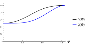
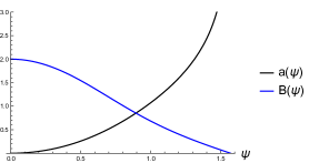
Figure 1: The profile functions in eq. (3.17) as a function of $\psi$, see eq. (2.27). Here we set $b=1$ and $\frac{e^{2}}{16\pi G}=1$. We plot also the magnetic field $B$.

3.2 Phase diagram

The relation between $b$ and the integration constant $\tilde{a}$ in eq. (3.2) is

$$4\pi G\,\frac{\tilde{a}^{2}}{e^{2}}=\frac{b}{(1+b)^{2}}\equiv s(b)\,.$$ (3.19)

Note that the function $s(b)$ has as maximum $\frac{1}{4}$ for $b=1$. Let us denote by

$$\tilde{a}_{c}=\frac{e}{\sqrt{16\pi G}}$$ (3.20)

the value of $\tilde{a}$ which corresponds to $b=1$. For $\tilde{a}<\tilde{a}_{c}$ there are two different solutions of eq. (3.19) for $b$ with a given $\tilde{a}$, while for $\tilde{a}>\tilde{a}_{c}$ there are no solutions for $b$. As a consequence, we find that $\tilde{a}_{c}$ is a maximum value for the external current $\tilde{a}$ for the solution in eq. (3.17).

The solution in eq. (3.17) has the following special limits

• The value $b=0$ correspond by definition to the AdS soliton [11], which in three dimensions is the same as global AdS₃. This can be checked as follows. For large $x$, we can approximate $W_{0}(x)\approx\log x$. In this limit, from eq. (3.12), we find

  $$\lim_{b\to 0}\,\frac{\tilde{r}^{2}}{r_{h}^{2}}=r^{2}+1\,,$$ (3.21)

  which gives, using eqs. (3.17), $h=g=1$.

• At large $b$ the solution approaches AdS₃ in the Poincaré patch. In this case, we have that $h=1$ except a small region nearby origin and

  $$g\approx\frac{(r^{2}+\frac{1}{b})b^{2}}{\left(1+b\right)^{2}}\frac{1}{1+r^{2}}\approx\frac{r^{2}+\frac{1}{b}}{r^{2}+1}\,,$$ (3.22)

  which, for $b\to\infty$, is indeed the AdS Poincaré patch.

In the left panel of figure 2 we plot $a_{0}$ as a function of the source $\tilde{a}$. In the right panel of figure 2 we plot the energy density, computed using eq. (2.5), as a function of the source $\tilde{a}$. The solution with $b>1$ always has higher energy compared to the one with $b<1$ with the same value of the current.

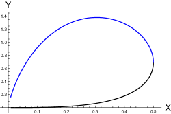
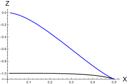
Figure 2: Left: plot of $Y=\frac{\sqrt{4\pi G}}{e}\,a_{0}$ as a function of $X=\frac{\sqrt{4\pi G}}{e}\,\tilde{a}=\frac{\sqrt{b}}{1+b}$. We set for simplicity the scale $r_{a}=1$. Right: we plot $Z=16\pi G\,\mathcal{E}$ as a function of $X$. The values for solution with $b<1$ and the one with $b>1$ are shown in black and in blue, respectively.

Global AdS corresponds to the vacuum of a CFT on a circle, with antiperiodic boundary conditions for the fermions, which give rise to the negative energy due to Casimir effect, see [11]. Poincaré patch has instead zero energy, because there the dual CFT has periodic boundary conditions for fermions, which do not break supersymmetry. So, we can argue by continuity that the $b<1$ branch corresponds to a phase with antiperiodic boundary conditions for fermions, while the $b>1$ branch to a phase with periodic ones. The critical value $\tilde{a}=\tilde{a}_{c}$ is the bifurcation point between the two phases.

There are some similarities with the AdS₄ Melvin solution, discussed in [66, 67]. Also in AdS₄ there are two different solutions for the same value of the source for the $U(1)$ gauge field below the critical value, see [67]. The two branches of the solution, for vanishing $A_{\mu}$, tend to the AdS soliton and to the Poincaré patch, respectively. Note that, in higher dimensions, the source (with Dirichlet boundary conditions) is the asymptotic value of $a(r\to\infty)=a_{0}$, while in AdS₃ we take as source the logarithmic falloff of $a$, which is given by $\tilde{a}$. In higher dimensions, the Poincaré AdS background provides a solution with arbitrary large source $a_{0}$. In AdS₃ we do not find any solution with source $\tilde{a}>\tilde{a}_{c}$, see eq. (3.20).

4 Black holes

In the previous section we have shown that the model in eq. (2.1) does not admit any black hole solutions with a non-zero magnetic field and vanishing scalar hair. In this section we will study black hole solutions with a non-zero scalar hair. We find that the Little-Parks periodicity is realized in the boundary dual of these black hole solutions.

The black hole horizon is where the $g(r_{h})=0$. The location of the horizon $r_{h}$ is a free parameter of the solution. The black hole Hawking temperature $T$ is

$$T=\frac{(1+r_{h}^{2})\,g^{\prime}(r_{h})}{4\pi}\,,$$ (4.1)

where $\psi_{h}$ denotes the horizon in the $\psi$ coordinates in eq. (2.27). Assuming that the temperature is not vanishing, from eqs. (2.15) we find that we should impose the following conditions at the horizon in order to avoid singularities

$$H^{\prime}(r_{h})=H(r_{h})\,\frac{h(r_{h})}{g^{\prime}(r_{h})}\,\left(\frac{(n-a(r_{h}))^{2}}{r_{h}^{2}(1+r_{h}^{2})}+\frac{m^{2}}{1+r_{h}^{2}}\right)\,,$$

$$a^{\prime}(r_{h})=2e^{2}\frac{h(r_{h})}{(1+r_{h}^{2})\,g^{\prime}(r_{h})}\,H^{2}(r_{h})\,(a(r_{h})-n)\,.$$ (4.2)

The zero temperature limit needs a more careful analysis, see section 4.3.

In condensed matter physics, the Little-Parks effect [34] consists in a periodic behavior of the current flowing in a superconducting ring as a function of the magnetic flux which is applied in the perpendicular direction. Let us denote by $\varphi$ the compact direction of the cylinder. In the Ginzburg-Landau theory, let us denote by $a_{\mu}$ the gauge field, by $D_{\mu}=\partial_{\mu}-ia_{\mu}$ the covariant derivative, by $v$ the vacuum expectation value of the order parameter $\phi=v\,e^{in\varphi}$. The superconducting current is proportional to

$${\rm Im}(\phi^{*}D_{\varphi}\phi)=(a_{\varphi}-n)v^{2}\,.$$

The Little-Parks effect is realized by the invariance $n\to n+p$ and $a_{\varphi}\to a_{\varphi}+p$ with integer $p$. The same invariance holds in the black hole phase, as studied in [32, 33] for the higher dimensional AdS spacetime. Both the equations of motion eq. (2.15) and the horizon boundary conditions eq. (4) are indeed invariant under the shift

$$n\to n+p\,,\qquad a(r)\to a(r)+p\,,$$ (4.3)

where $p$ is an arbitrary integer.

4.1 Solutions with vanishing external current

If we set $a=n$ as a boundary condition at the horizon, from the equations of motion eqs. (2.15) we find that $a$ remains constant. In appendix B we prove that, for vanishing external current $\tilde{a}$, the profile function $a$ is identically equal to $n$ for the black hole solution. This means that the magnetic flux in eq. (2.39) is quantized for the black hole solution with $\tilde{a}=0$. This is true even if there is no magnetic field in the solution, because the flux has fallen into the singularity, leaving a quantized Wilson line outside the horizon.

Specializing eqs. (2.15) with $a=n$, we find

$$\frac{d}{dr}\left(q\,rH^{\prime}\right)=r\,h\,H\,m^{2}\,,\qquad\frac{h^{\prime}}{h}=16\pi G\,r\,{H^{\prime}}^{2}\,,\qquad q^{\prime}=h\,r\,\left(2-m^{2}\,{16\pi G}\,H^{2}\right)\,.$$ (4.4)

Note that the system in eq. (4.4), is independent from the coupling $e$ and from the winding number $n$.

A special class of solutions of eq. (4.4) with vanishing scalar hair is provided by the BTZ black hole, see eq. (3.3). The mass, the temperature and the entropy are

$$M=2\pi\,\mathcal{E}=\frac{\mu}{8G}\,,\qquad T=\frac{\sqrt{\mu}}{2\pi}\,,\qquad S=\frac{\pi\sqrt{\mu}}{2G}\,,$$ (4.5)

where $\mu=r_{h}^{2}$. The free energy is

$$F=M-TS=-\frac{\pi^{2}}{2}\frac{1}{G}T^{2}\,.$$ (4.6)

There is a Hawking-Page transition between global AdS and the BTZ black hole [70] at the critical temperature

$$T_{0}=\frac{1}{2\pi}\,.$$ (4.7)

The BTZ background provides a good approximation nearby the critical temperature for the scalar condensation, because $H$ is small in that regime. Considering a small perturbation of the scalar field $H$ in eqs. (4.4) and neglecting the gravitational backreaction, we find a linear equation for $H(r)$

$$H^{\prime\prime}=-\frac{3r^{2}-\mu}{r(r^{2}-\mu)}H^{\prime}+\frac{m^{2}}{(r^{2}-\mu)}H\,,$$ (4.8)

which, combined with the boundary conditions in eq. (4) admits the exact solution

$$H=\frac{\Gamma(\sqrt{m^{2}+1})\left(\frac{r^{2}}{\mu}\right)^{-\frac{\Delta_{-}}{2}}\,_{2}F_{1}\left(\frac{\Delta_{-}}{2},\frac{\Delta_{-}}{2};\Delta_{-};\frac{\mu}{r^{2}}\right)}{\Gamma\left(\frac{\Delta_{+}}{2}\right)^{2}}$$

$$\quad+\frac{\Gamma(-\sqrt{m^{2}+1})\left(\frac{r^{2}}{\mu}\right)^{-\frac{\Delta_{+}}{2}}\,_{2}F_{1}\left(\frac{\Delta_{+}}{2},\frac{\Delta_{+}}{2};\Delta_{+};\frac{\mu}{r^{2}}\right)}{\Gamma\left(\frac{\Delta_{-}}{2}\right)^{2}}\,.$$ (4.9)

We show a plot of eq. (4.9) in figure 3. The solution can be extrapolated also inside the horizon. Nearby $r=0$, we have a logarithmic singularity in the behaviour of the scalar field in eq. (4.9)

$$H\approx-\frac{2}{\mu^{\frac{\Delta_{-}}{2}}}\,\frac{\Gamma(\frac{\Delta_{+}}{2})}{\Gamma(\sqrt{1+m^{2}})\,\Gamma\left(\frac{\Delta_{-}}{2}\right)}\,\log\,r\,.$$ (4.10)

There is a similar singularity in the black hole solution studied in [46].

Figure 3: Profile function $H(\psi)$ in eq. (4.9) for $m^{2}=-0.9$ and $r_{h}=1$. The solid and the dashed parts of the curve correspond to the part outside and inside the horizon, respectively.

At large $r$, from the exact solution we find the expansion

$$H\approx\frac{\Gamma\left(\sqrt{m^{2}+1}\right)}{\Gamma\left(\frac{\Delta_{+}}{2}\right)^{2}}\left(\frac{\sqrt{\mu}}{r}\right)^{\Delta_{-}}+\frac{\Gamma\left(-\sqrt{m^{2}+1}\right)}{\Gamma\left(\frac{\Delta_{-}}{2}\right)^{2}}\left(\frac{\sqrt{\mu}}{r}\right)^{\Delta_{+}}\,,$$ (4.11)

which corresponds to the double trace coupling

$$\kappa=\frac{\Gamma\left(-\sqrt{m^{2}+1}\right)\Gamma\left(\frac{\Delta_{+}}{2}\right)^{2}}{\Gamma\left(\sqrt{m^{2}+1}\right)\Gamma\left(\frac{\Delta_{-}}{2}\right)^{2}}\,\left(\frac{T}{T_{0}}\right)^{2\sqrt{m^{2}+1}}\,,$$ (4.12)

where we used $\mu=4\pi^{2}T^{2}$. The behavior in eq. (4.12) follows from dimensional analysis, using the dimension of the coupling $\kappa$ in the CFT, see eq. (2.33).

In correspondence of the temperature $T_{0}$ of the Hawking-Page transition, the value of $\kappa$ in eq. (4.12) is the same as the critical value $\kappa_{c1}$ for $n=0$, as we will show in the next section, see $\kappa_{v}$ in eq. (5.5). We can interpret eq. (4.12) as the critical coupling $\kappa$ for condensation, as a function of temperature.

If we want to include the gravitational backreaction of the scalar $H$ on the metric, we have to solve the system eq. (4.4) numerically, see appendix A for details. In figure 4 we show an example of solution with $\kappa=-1$ and $r_{h}=1$. Nearby $r\to 0$, the behavior of the solution is

$$H\approx-C_{H}\,\log r\,,\qquad h\approx h_{0}\,r^{16\pi G\,C_{H}^{2}}\,,\qquad g\approx g_{0}(1-r^{2})\,,$$ (4.13)

for some opportune constants $C_{H}$, $h_{0}$ and $g_{0}$.

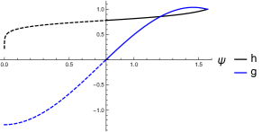
Figure 4: Example of black hole solution with $\tilde{a}=0$. Here we set $r_{h}=1$, $m^{2}=-0.9$, $G=0.1$, $\kappa=-1$. The solid and the dashed part of the curve corresponds to the part outside and inside the horizon, respectively. The profile function $a$ is identically equal to the winding number $n$ of the scalar field. The magnetic and electric fields vanish.

For fixed temperature, in the macrocanonical ensemble the thermodynamically favored solution is the one with lower free energy

$$F=U-TS=2\pi\left(\mathcal{E}-\,\frac{T\,r_{h}}{4\,G}\right)\,.$$ (4.14)

In figure 5 we show the results of numerical calculations for the free energy of the black hole solution as a function of the temperature, for fixed values of $\kappa$. Note that, at low enough temperature, the hairy black hole has a lower free energy than the BTZ solution. From these plots we can check that, at the critical temperature given by eq. (4.12), the hairy solution and the BTZ black hole have the same free energy. Above the critical temperature, the hairy black hole with a given $\kappa$ no longer exists.

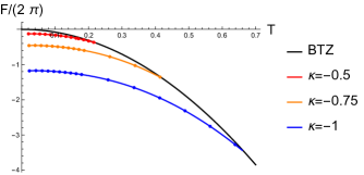
Figure 5: Free energy $\frac{F}{2\pi}$ as a function of temperature $T$ for the hairy black hole solutions with $\tilde{a}=0$, for a few values of $\kappa$. Here we set $m^{2}=-0.9$ and $G=0.1$.

4.2 Solutions with non-zero external current

In figure 6 we show an example of numerical solution for the black hole with scalar hair for non-zero external current $\tilde{a}$. In this case, the black solution has a non-zero magnetic field outside the horizon. Note that the magnetic field vanishes inside the horizon. Inside the horizon, instead there is a non-vanishing electric field because $r$ becomes a timelike coordinate, see figure 7. In the Ampère law, the term involving the curl of the magnetic field is zero inside the horizon and is replaced by the time derivative of the electric field, which comes from Maxwell’s displacement current term.

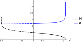
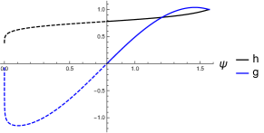
Figure 6: Example of BH solution with non-zero current $\tilde{a}$.

Figure 7: Plot of $B^{2}\propto F_{\mu\nu}F^{\mu\nu}$ for the solution in figure 6. Inside the horizon, the magnetic field vanishes and it is replaced by an electric field. The solid and the dashed part of the curve corresponds to the square of the magnetic field outside and to the square of the electric field inside the horizon, respectively.

In the left panel of figure 8 we show $\tilde{a}$ as a function of $a_{0}$, extracted from a class of solutions with constant $\kappa$ and $T$. This illustrates the Little-Parks periodicity in eq. (4.3). In the right panel of figure 8 we show a plot of the scalar condensate, which is suppressed by the presence of the external current. We find that there is a maximum value for $\tilde{a}$, as in the case of vanishing scalar field studied in section 3, see eq. (3.20).

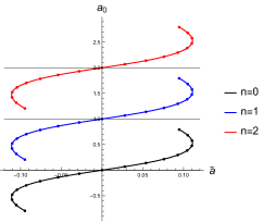
Figure 8: On the left panel, we show the expectation value $a_{0}$ as a function of the external current $\tilde{a}$. For a given winding, we checked that the solution with lower $|a_{0}-n|$ has a lower free energy. On the right panel we plot the condensate $\alpha_{H}$ as a function of $\tilde{a}$. The presence of a current tends to suppress the VEV of the scalar condensate. Here we use the numerical values $e=1$, $G=0.1$, $T=0.2$, $\kappa=-1$.

4.3 Zero temperature limit

In this section, we will consider the low temperature limit of the black hole solution with vanishing external current $\tilde{a}=0$. The zero temperature limit is interesting, because it is recovered in the transition from the soliton regime, which we will discuss in section 5.3. We will find a zero temperature limit which is similar to the one found for the AdS₄ holographic superconductor with $m^{2}<0$ in [35].

Let us first neglect the gravitational backreaction, and solve the equation for $H$ on the zero temperature limit of the BTZ solution, which is the Poincaré patch. Setting $\mu=0$ in eq. (4.8), we find the solutions

$$H=A\,r^{-\Delta_{-}}+B\,r^{-\Delta_{+}}\,,$$ (4.15)

where $A$ and $B$ are integration constants. For all the values of the integration constants, the scalar field $H$ diverges at the origin. We will check that, including the effect of the gravitational backreaction, the divergence in $H$ becomes milder.

Let us first prove that, in the zero temperature limit, the horizon radius (which is defined by the equation $g(r_{h})=0$) approaches $r_{h}\to 0$. From eq. (4.1), we find that in the zero temperature limit we have $g^{\prime}(r_{h})=0$, which is equivalent to $q^{\prime}(r_{h})=0$. Using the equations of motion eq. (4.4), we find that for $r=r_{h}$ the following quantity should vanish

$$h\,r\left(2-{16\pi G}\,m^{2}\,H^{2}\right)=0\,.$$ (4.16)

Moreover $h(r_{h})\neq 0$, otherwise there would be a singularity on the horizon. Because $m^{2}$ is negative, we have that $r_{h}$ then should vanish. In the zero temperature limit, the black hole approaches a zero entropy field configuration as in [35].

Let us investigate the behavior of the zero temperature limit of the black hole nearby $r=0$. We will check that $H$ diverges for $r\to 0$. We can approximate eq. (4.4) as follows

$$\frac{d}{dr}\left(q\,rH^{\prime}\right)=r\,h\,H\,m^{2}\,,\qquad\frac{h^{\prime}}{h}=16\pi G\,r\,{H^{\prime}}^{2}\,,\qquad q^{\prime}=-m^{2}\,{16\pi G}\,r\,H^{2}\,h\,.$$ (4.17)

Combining the first and the last equations in the system in eq. (4.17), we find

$$-m^{2}\,{16\pi G}\,r^{2}\,H^{2}\,H^{\prime}+\frac{q}{h}\,(H^{\prime}+rH^{\prime\prime})=r\,H\,m^{2}\,.$$ (4.18)

Let us assume that in eq. (4.18) the term $\frac{q}{h}(H^{\prime}+rH^{\prime\prime})$ can be neglected (the self-consistency of this assumption can be checked at the end of the calculation). With this approximation, we find

$$-{16\pi G}\,r\,H\,H^{\prime}\approx\,1\,,$$ (4.19)

which gives the approximate solution nearby $r\to 0$

$$H\approx\sqrt{\frac{-\log r}{8\pi G}}\,.$$ (4.20)

From the other equations in eq. (4.17), we find

$$h\approx\frac{C}{\sqrt{-\log r}}\,,\qquad q\approx-m^{2}\,C\,r^{2}\,\sqrt{-\log r}\,,$$ (4.21)

where $C>0$ is an integration constant. From these expression, we can check that the term $\frac{q}{h}(H^{\prime}+rH^{\prime\prime})$ can be neglected in eq. (4.18).

From eq. (4.21), the metric takes the following form nearby $r\to 0$,

$$ds^{2}\approx r^{2}(-{d\tilde{t}}^{2}+d\varphi^{2})+\frac{dr^{2}}{(-m^{2})r^{2}(-\log r)}\,,$$ (4.22)

where $\tilde{t}=\sqrt{-m^{2}}\,C\,t$. There is a mild null singularity at $r\to 0$, which can be detected by the Ricci scalar

$$R\approx-6m^{2}\,\log r\,.$$ (4.23)

We show an example of solution in figure 9.

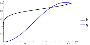
Figure 9: Zero temperature limit of the black hole solution. Here we set $m^{2}=-0.9$, $G=0.1$, $\kappa=-1$.

5 Solitons with scalar hair

In this section we study soliton solutions with scalar hair with external current $\tilde{a}=0$. In section 5.1 we discuss an analytical solution which is exact for $G=e=0$ and which provides a good approximation in the regime of small $\alpha_{H}$. It turns out that, for a backreacted vacuum solution, $\kappa$ is a monotonic function of $\alpha_{H}$. For the vacuum ($n=0$), the exact solution for $G=e=0$ provides a good approximation nearby the critical $\kappa=\kappa_{c1}$ for the scalar condensation. For a vortex with $n\geq 1$, $\kappa$ instead is not a monotonic function of $\alpha_{H}$ and so the solution in section 5.1 does not provide a good approximation at the threshold of the scalar condensation.

For $e,G\to 0$, the equation of motion for $H$ is linear and so $\kappa$ is a constant as a function of $\alpha_{H}$. In this limit, the double trace coupling $\kappa$ depends just on the winding $n$, thus different windings correspond to different values of $\kappa$. In order to compare the energy of solitons with different windings and with the same value of the coupling $\kappa$, we need to solve the equations including backreaction. In section 5.2 we discuss some numerical results.

It is interesting that for fixed $G$, $e$ and $n\geq 1$ there is a second critical value $\kappa=\kappa_{c2}$ below which no soliton solution can be found. For values just above $\kappa_{c2}$, the soliton tends to develop a horizon at $r=r_{h}$, which is detected by the vanishing of $g(r_{h})$. We discuss this regime in section 5.3.

In the limit of large $e$ and fixed $G$, $\kappa$ and $n\geq 1$, the magnetic flux is concentrated in a small region nearby $r=0$. We may wonder if there is a critical value of $e$ above which the soliton becomes a black hole. In appendix C we present evidences that this is not the case. Indeed, as we have seen in section 3, no black hole solution can be found with vanishing scalar and non-vanishing magnetic field.

5.1 An analytical solution in global AdS

In this section, we discuss a solution of the equations of motion in global AdS, which is valid in the mass range $-1\leq m^{2}\leq 0$ and exact for $G=e=0$. In this limit, it is consistent to set $a=0$. From eq. (2.15), we find a linear equation for $H(r)$

$$H^{\prime\prime}=-\frac{1+3r^{2}}{r\left(1+r^{2}\right)}H^{\prime}+\frac{n^{2}+m^{2}r^{2}}{r^{2}\left(1+r^{2}\right)}H\,,$$ (5.1)

which in general has the following exact solution

$$H(r)=\frac{{\Gamma\left(\frac{n+\Delta_{+}}{2}\right)}^{2}}{\Gamma\left(\sqrt{1+m^{2}}\right)\Gamma(n+1)}\,r^{n}\,_{2}F_{1}\left(\frac{n+\Delta_{-}}{2},\frac{n+\Delta_{+}}{2};n+1;-r^{2}\right)\,,$$ (5.2)

normalized with $\alpha_{H}=1$. Plots for different $n$ are shown in the left panel of figure 10. These solutions correspond to eigenvectors of the laplacian operator in AdS, see for example [69].

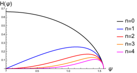
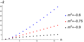
Figure 10: Left panel: solutions $H$ in eq. (5.2), plotted as a function of $\psi=\arctan r$, for a few values of $n$ and $m^{2}=-0.9$. Right panel: Plot of $-\hat{\kappa}(n)$ for a few values of $m^{2}$.

We can express the double trace coupling corresponding to these solutions as

$$\hat{\kappa}(n)=\frac{\beta_{H}}{\alpha_{H}}=\frac{\Gamma\left(-\sqrt{1+m^{2}}\right)}{\Gamma\left(\sqrt{1+m^{2}}\right)}\left[\frac{\Gamma\left(\frac{n+\Delta_{+}}{2}\right)}{\Gamma\left(\frac{n+\Delta_{-}}{2}\right)}\right]^{2}\,.$$ (5.3)

Note that the coupling $\hat{\kappa}$ is negative, as expected in order to achieve spontaneous symmetry breaking. We can use the approximate formula at large $n$

$$\hat{\kappa}(n)\approx\frac{\Gamma\left(-\sqrt{1+m^{2}}\right)}{\Gamma\left(\sqrt{1+m^{2}}\right)}\left(\frac{n}{2}\right)^{2\sqrt{1+m^{2}}}\,,$$ (5.4)

which can be derived from the Stirling approximation. For the special value $m^{2}=-\frac{3}{4}$, we have $\hat{\kappa}(n)\approx-n$. In the zero mass limit we have $\hat{\kappa}(n)\propto-n^{2}$. In the Breitenlohner-Freedman limit $m^{2}\to-1$, we have $\hat{\kappa}(n)\propto-n^{0}$. See the right panel of figure 10 for a plot of $\hat{\kappa}$ as a function of $n$.

5.2 Numerical solutions

In order to study solitonic solutions with non-zero $e$ and $G$, we have to use numerical methods, see appendix A. If we neglect the gravitational backreaction, the coupling $e$ by itself does not introduce any non-linearity for the vacuum. In this case $a$ vanishes and the solution for $H$ is given by eq. (5.2) with $n=0$ for every value of $e$. The multitrace coupling $\kappa$ is independent of $\alpha_{H}$ and is given by $\hat{\kappa}$ in eq. (5.3). For $n\geq 1$, there is instead a dependence of $\kappa$ on $\alpha_{H}$, see figure 11. Still, we find that for the vortex configuration $\kappa$ is always lower than the vacuum case. Without including gravitational backreaction, it is not possible to compare the properties of the vortex solution with a vacuum solution with the same choice of double trace coupling $\kappa$.

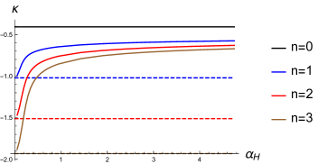
Figure 11: $\kappa$ as a function of $\alpha_{H}$ for the vacuum $n=0$ and for the $n=1,2,3$ vortices. Here we set $m^{2}=-0.9$ and $e=10$ and we neglect the gravitational backreaction, solving the equations of motion on the global AdS metric. The dotted lines correspond to $e=0$, where $\kappa$ does not depend on $\alpha$.

In figure 12 we show $\kappa$ as a function of $\alpha_{H}$ for a class of solitonic vortex solutions with backreaction, for a few values of the winding number $n$. Note that $\kappa$, which is always negative, has a maximum $\kappa_{c1}$ as a function of $\alpha_{H}$. For the vacuum $n=0$ this maximum corresponds to $\alpha_{H}\to 0$ and to

$$\kappa_{v}=\kappa_{c1}(0)=\hat{\kappa}(0)=\frac{\Gamma\left(-\sqrt{1+m^{2}}\right)}{\Gamma\left(\sqrt{1+m^{2}}\right)}\left[\frac{\Gamma\left(\frac{\Delta_{+}}{2}\right)}{\Gamma\left(\frac{\Delta_{-}}{2}\right)}\right]^{2}$$ (5.5)

given in eq. (5.3). For $\kappa$ just below $\kappa_{c1}$, we find, for $n\geq 1$, two different vortex solutions, with different values of $\alpha_{H}$. We checked that among these solutions, the one with larger $\alpha_{H}$ has always lower energy, and so it is energetically favored. In the following we will always refer to the lower energy solution. In figure 13 we show some examples of solutions.

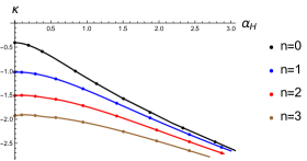
Figure 12: $\kappa$ as a function of $\alpha_{H}$ for the vacuum and $n=1,2,3$ vortices. Here we set $m^{2}=-0.9$ and $G=0.1$. In the left panel we set $e=0$, while in the right panel we consider $e=10$.

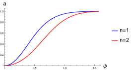
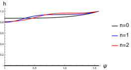
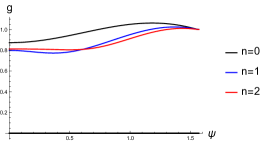
Figure 13: Soliton solutions for $n=0,1,2$. Here we set $m^{2}=-0.9$, $e=10$, $G=0.1$ and $\kappa=-1$. The three solution have $\alpha_{H}=0.840$, $\alpha_{H}=0.738$ and $\alpha_{H}=0.604$, respectively. We have $\mathcal{E}(n=1)-\mathcal{E}(n=0)=0.301$ and $\mathcal{E}(n=2)-\mathcal{E}(n=1)=0.307$.

The magnetic flux $\mathcal{F}$ of the solution with vanishing source $\tilde{a}$ is

$$\mathcal{F}=\frac{2\pi}{e}\,a(\infty)=\frac{2\pi}{e}\,a_{0}\,,$$ (5.6)

see eq. (2.39). While in flat space the flux of a vortex is quantized, otherwise its energy is infinite, this is not necessarily the case in the AdS setting studied in this paper, see the discussion nearby eq. (2.40). Note that the magnetic flux instead is quantized for the black hole solutions with $\tilde{a}=0$, as we proved in appendix B.

In figure 14 we plot the vortex flux as a function of the scalar expectation value $\alpha_{H}$. We see that $a_{0}$ tends to approach the winding number $n$ for large enough $\alpha_{H}$, which correspond to large enough $|\kappa|$. In this limit, the quantization of the flux holds in a similar way as in flat space. Another limit in which the quantization of the flux holds is the one of large $e$ with fixed $\kappa$.

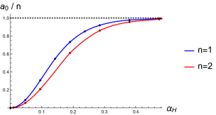
Figure 14: The normalized flux $\frac{a_{0}}{n}$ as a function of $\alpha_{H}$ for the $n=1$ and $n=2$ vortices. Here we set $e=10$, $m^{2}=-0.9$ and $G=0.1$.

5.3 Approaching the critical solution

Let us fix $e$ and $G$ and decrease the negative coupling $\kappa$. From figure 12, we see that $\alpha_{H}$ increases. As a consequence, the scalar field $H$ in the interior of the geometry also tends to increase. For $n\geq 1$, the magnetic field is localized in a increasingly narrow region nearby $r=0$. Intuitively, if some energy is concentrated inside a region whose size approaches the Schwarzschild radius, a black hole horizon will form. For this reason, we expect that it exists a critical value of the coupling $\kappa$, which we denote by $\kappa_{c2}$, above which no soliton solution with a given winding $n\geq 1$ can exist, due to black hole horizon formation. A similar transition between monopole solutions and black holes was investigated in flat space in [22, 23].

In order for the critical solution to exist, we need that, for a certain value of $r=r_{0}$, the function $q(r)$ has a positive minimum $q(r_{0})$ which tends to zero, in such a way that $q^{\prime}(r)<0$ for $r<r_{0}$. The minimum condition $q^{\prime}(r_{0})=0$, with the horizon condition $q(r_{0})=0$, tells us that the black hole should have vanishing temperature, see eq. (4.1). In section 4.3 we have found that the zero temperature condition implies that the radius $r_{h}$ of the horizon of the black hole vanishes, and so that the entropy is zero. The zero temperature limit of the black hole solution corresponds to a zero entropy configuration, where the horizon lies on top of a mild logarithmic curvature singularity at $r_{h}=0$.

Let us inspect the equation for $q$ in eq. (2.15)

$$q^{\prime}=h\left(2r-{16\pi G}\left(\frac{(a-n)^{2}}{r}+m^{2}r\right)\,H^{2}\right)\,.$$ (5.7)

From this expression, we find $q^{\prime}(r)>0$ if $m^{2}$ is negative and $n=0$, because in this case $a=0$. No critical solution can exist for $n=0$. As a consequence, for $n=0$ a soliton solution without horizon always exists for every value of $\alpha_{H}$. This is consistent with the numerical solutions. Instead, for higher windings $n\geq 1$ we can always find a region, nearby $r=0$, where

$$\frac{(a-n)^{2}}{r^{2}}>-m^{2}\,,$$

in such a way that $q^{\prime}$ might become negative. Critical solutions may then exist for $n\geq 1$.

In order to give a criterium for the formation of a horizon, let us integrate eq. (2.21) from $r=0$ to the would be horizon $r_{0}$. Assuming that $q$ has a positive minimum at $r=r_{0}$, we find

$$16\pi G\int_{0}^{r_{0}}\rho\,r\,dr\leq r_{0}^{2}+1\,.$$ (5.8)

If the integral of $\rho$ inside a ball with radius $r_{0}$ saturates the bound (5.8), a horizon forms. See figure 15 for an example of nearly critical solution for $n=1$. We checked numerically that eq. (5.8) tends to be saturated for the critical solution.

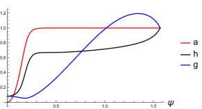
Figure 15: Example of nearly critical soliton solution with $n=1$. Here we set $e=10$, $m^{2}=-0.9$, $G=0.1$, $\kappa=-2.735$, $\alpha_{H}=3.220$.

For fixed $e$ and $G$, a vortex soliton with a given $n\geq 1$ exists just in a finite window of multitrace coupling $\kappa$. There is an upper bound given by $\kappa_{c1}$, see figure 12. There is also a lower bound given by $\kappa_{c2}$, otherwise the soliton tends to develop a horizon at $r_{h}\to 0$, as shown in figure 15. For $e=10$ and $G=0.1$, we have $\kappa_{c1}=-0.8$ and $\kappa_{c2}=-2.75$.

In appendix C we briefly consider the large $e$ limit with fixed $\kappa$. In this case, we do not find any critical $e$ for which the soliton solution tends to develop a horizon.

6 Conclusions

In this paper, we studied various soliton and black hole solutions in AdS Einstein gravity with a Maxwell and a charged scalar field. Here we summarize our results about the phase diagram with vanishing external current $\tilde{a}$ as a function of the temperature $T$, the double trace coupling $\kappa$, and the winding number $n$. At low enough temperature, the soliton solution can have lower free energy compared to the black hole. This gives rise to a first order phase transition, which is analog to the one studied by Hawking and Page [9]. Moreover, the double trace coupling $\kappa$ can trigger the condensation of the scalar order parameter, giving rise to a second order phase transition to a superconducting phase [17]. As in [13, 14], we can have a total of four possible phases, corresponding to a smooth soliton and black hole with or without the presence of scalar hair. For zero winding number $n=0$ the phase diagram is independent of the bulk $U(1)$ gauge coupling $e$, because the solutions have vanishing field strength $F_{\mu\nu}$. In this case, a soliton exists for every value of $\kappa<\kappa_{v}$, see eq. (5.5). We show the phase diagram in figure 16. For $\kappa\geq\kappa_{v}$, there is no scalar condensation and there is the Hawing-Page first order phase transition at the temperature $T_{0}=\frac{1}{2\pi}$. For $\kappa<\kappa_{v}$, the hairy soliton solution has a lower free energy at low enough temperature. At a critical temperature $T_{c1}$, which depends on the Newton constant $G$ and that can be found numerically by comparing the free energy of the black hole and of the soliton phase, there is a first order transition to the hairy black hole phase. From numerical calculations, we find that $T_{c1}$ is an increasing function of $|\kappa|$, see figure 16. At a higher temperature $T_{c2}$, which is independent of $G$ and that can be found by solving eq. (4.12) to be

$$T_{c2}=T_{0}\left[\frac{\Gamma\left(\sqrt{m^{2}+1}\right)\Gamma\left(\frac{\Delta_{-}}{2}\right)^{2}}{\Gamma\left(-\sqrt{m^{2}+1}\right)\Gamma\left(\frac{\Delta_{+}}{2}\right)^{2}}\,\kappa\right]^{\frac{1}{2\sqrt{m^{2}+1}}}\,,$$ (6.1)

there is a second order phase transition to a non-superconducting phase, which is described by the BTZ black hole solution. The fact that for $\kappa=\kappa_{v}$ the critical temperature $T_{c2}$ in eq. (6.1) is equal to $T_{0}$ provides evidence for the quadruple point in the phase diagram in figure 16. This is a different feature compared to [13, 14], where the quadruple point can be realized just for a fine-tuned choice of the couplings.

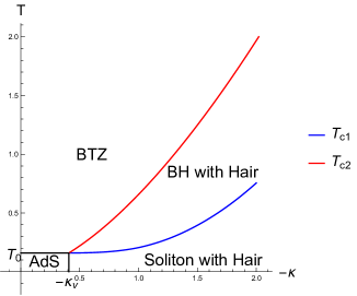
Figure 16: Phases diagram for $\tilde{a}=0$ in the $(-\kappa,T)$ plane for for the vacuum solution $n=0$, for $m^{2}=-0.9$ and $G=0.1$.

For non-zero winding $n$, a soliton solution exists just in a specific window of the double trace coupling $\kappa_{c2}\leq\kappa\leq\kappa_{c1}$ which depends both on the couplings $G$, $e$ and on the winding $n$. For example, for $n=1$ and for the value of the couplings $e=10$ and $G=0.1$ we have $\kappa_{c1}=-0.8$ and $\kappa_{c2}=-2.75$. We show the phase diagram in figure 17. For a value of $\kappa$ below $\kappa_{v}$ and outside the window $\kappa_{c2}\leq\kappa\leq\kappa_{c1}$, there are just two phases, described by the hairy black hole and by the BTZ solution. Instead, in the window $\kappa_{c2}\leq\kappa\leq\kappa_{c1}$, there is also the soliton vortex phase. In the low temperature limit, it can happen that the vortex has a lower free energy than the black hole, see the blue region in figure 17.

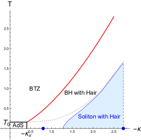
Figure 17: Phase diagram for the vortex solution with $n=1$, for $m^{2}=-0.9$, $G=0.1$, and $e=10$. The two blue points mark the values $\kappa_{c1}$ and $\kappa_{c2}$, which correspond to the maximum and minimum value of $\kappa$ for which a solitonic vortex solution exists. The solid blue line corresponds to the first order phase transition between soliton and black hole, due to the change of the minimum of the free energy (for comparison, the same transition is shown for $n=0$ in a black dotted line). The dashed blue line is the border of the region where the soliton with $n=1$ does not exist, because a black hole horizon tends to form.

In the case of vanishing scalar hair, we also studied the phase diagram with non-zero external current $\tilde{a}$, see section 3. For a given value of $\tilde{a}$ below a critical value $\tilde{a}_{c}$ given in eq. (3.20), we find that there are two solutions. For vanishing $\tilde{a}$ the two solutions correspond to global AdS and to the Poincaré patch. For the critical value $\tilde{a}_{c}$ the two branches of solutions coincide, see figure 2. We find that the branch which is continuously connected to global AdS has always a lower energy compared to the branch which is continuously connected to the Poincaré patch. An analogous phase diagram has been investigated in higher dimensions in [66, 67].

In the hairy black hole phase, we have found by numerical methods that there is also a maximum value of the current $\tilde{a}$, see figure 8. This is consistent with the presence of the Little-Parks periodicity, which is is realized by the shift symmetry in eq. (4.3), as in [32, 33]. In the soliton phase, instead, if we use regular boundary conditions at $r=0$, we find no evidence of Little-Parks periodicity. Violations of LP periodicity has been studied in the condensed matter literature, for example in small cylinders, when the size of the system is of the same order of magnitude of the coherence length of the superconductor, see [71, 72, 73].

Acknowledgments

The work of R. A., S. B., and G. N. is supported by the INFN special research project grant “GAST” (Gauge and String Theories). The work of N. Z. is supported by MEXT KAKENHI Grant-in-Aid for Transformative Research Areas A “Extreme Universe” No. 21H05184.

Appendix

Appendix A Numerical methods

In order to find numerical solutions to the equations of motion, it is useful to introduce the compact coordinate $\psi=\arctan r$. In this coordinates the metric of global AdS is

$$ds^{2}=\frac{1}{\cos^{2}\psi}\left(-\,hg\,dt^{2}+\frac{h}{g}d\psi^{2}+\sin^{2}\psi\,d\varphi^{2}\right)\,.$$ (A.1)

The equations of motion eq. (2.15) in the $\psi$ variable read

$$E_{H} =H^{\prime\prime}-\frac{1}{g}\left[\left((n-a)^{2}\csc^{2}\psi+m^{2}\sec^{2}\psi\right)h\,H-\left(g\,\csc\psi\,\sec\psi+g^{\prime}\right)H^{\prime}\right]=0\,,$$ (A.2)

$$E_{a} =a^{\prime\prime}-\frac{1}{g}\left[2e^{2}(a-n)\,h\,H^{2}\,\sec^{2}\psi+\left(g\,\csc\psi\,\sec\psi-g^{\prime}\right)a^{\prime}\right]=0\,,$$

$$E_{h} =h^{\prime}-{8\pi G}\,h\,\cos\psi\left(\cos\psi\cot\psi\,\frac{{a^{\prime}}^{2}}{e^{2}}+2\sin\psi\,{H^{\prime}}^{2}\right)=0\,,$$

$$E_{g} =g^{\prime}-\left[2\tan\psi\left(h-g\right)-{16\pi G}\,h\,\tan\psi\left((n-a)^{2}\cot^{2}\psi+m^{2}\right)H^{2}\right]=0\,,$$

where ^′ denotes the derivative with respect to $\psi$.

In the case of the black hole with scalar hair, we can find numerical solutions by solving directly eqs. (A.2) as a system of ODE, with boundary conditions at the horizon $\psi_{h}=\arctan(r_{h})$. In terms of the $\psi$ coordinate, the horizon boundary conditions in eq. (4) are

$$H^{\prime}(\psi_{h})=H(\psi_{h})\,\frac{h(\psi_{h})}{g^{\prime}(\psi_{h})}\,\left(\frac{(n-a(\psi_{h}))^{2}}{\sin^{2}\psi_{h}}+\frac{m^{2}}{\cos^{2}\psi_{h}}\right)\,,$$

$$a^{\prime}(\psi_{h})=2e^{2}\frac{h(\psi_{h})}{\cos^{2}\psi_{h}\,g^{\prime}(\psi_{h})}\,H^{2}(\psi_{h})\,(a(\psi_{h})-n)\,.$$ (A.3)

In the case of the soliton, it is a little subtle to solve the system of ordinary differential equations in eq. (2.15) numerically. The difficulties basically arise because the smooth solutions for $H$ and $a$ are fine-tuned as functions of boundary conditions. We solve the equations for $H$, $a$ with fixed $g,h$, using the relaxation method. We add an auxiliary time dependence to the profile functions $H(\psi,t)$ and $a(\psi,t)$ and we solve for the partial differential equations (PDE) system

$$\frac{\partial H}{\partial t}=E_{H}\,,\qquad\frac{\partial a}{\partial t}=E_{a}\,,$$ (A.4)

where $E_{H}$ and $E_{a}$ are in eq. (A.2). The vanishing of $E_{H}$ and $E_{a}$ is equivalent to the equations of motion for $H$ and $a$. We use the exact solution with $e=G=0$ in eq. (5.2) as an initial condition at $t=0$ for the PDE system. For the scalar $H$, we impose the boundary condition with fixed $\alpha_{H}$ at $\psi=\frac{\pi}{2}$, where $\alpha_{H}$ can be computed as follows

$$\alpha_{H}=\lim_{\psi\to\frac{\pi}{2}}\frac{(\tan\psi)^{1-2\sqrt{1+m^{2}}}}{2\sqrt{1+m^{2}}}\,[H(\psi)(\tan\psi)^{\Delta_{+}}]^{\prime}\cos^{2}\psi\,.$$ (A.5)

Then, we can extract $\beta_{H}$ by performing a fit on the tails of the solution. In order to study the vortex solution without gravitational backreaction, we set $h=g=1$, and we solve the PDE system in eq. (A.4).

In order to find solutions which include gravitational backreaction, we can first solve the ordinary differential equations (ODE) for the metric functions $h$ and $g$ in eq. (A.2) for fixed $H$ and $a$, given by the solution of eqs. (A.4) on global AdS background. We can then iterate the procedure several times, each time solving first the PDE for $H$ and $a$, and then again solving the ODE for $h$ and $g$. Each time we solve the ODE for $h,g$, we can monitor $E_{H}$ and $E_{a}$ for convergence. We continue until the procedure converges and $E_{H}$ and $E_{a}$ are small enough. When this procedure converges, we can find backreacted solutions with arbitrary accuracy.

Appendix B Proof that $a(r)=n$ for a black hole with zero external current

Here we prove that, for the black hole solution with zero external current $\tilde{a}=0$, we can set $a(r)=n$. The proof is analogous to the one of the scalar no-hair theorem [74, 23]. Let us suppose that it is not the case and then we will find a contradiction. Let us start from the second equation in the system in eq. (2.15) and multiply both sides by $a-n$

$$(a-n)\frac{d}{dr}\left(\frac{g\,(1+r^{2})}{r}a^{\prime}\right)=2e^{2}\frac{(a-n)^{2}}{r}\,h\,H^{2}\,.$$ (B.1)

We can write the above equality as

$$\frac{d}{dr}\left[(a-n)\left(\frac{g\,(1+r^{2})}{r}a^{\prime}\right)\right]={a^{\prime}}^{2}\left(\frac{g\,(1+r^{2})}{r}\right)+2e^{2}\frac{(a-n)^{2}}{r}\,h\,H^{2}\,.$$ (B.2)

By denoting the horizon radius $r_{h}$ as the most external zero of $g(r)$, we integrate

$$\int_{r_{h}}^{\infty}\frac{d}{dr}\left[(a-n)\left(\frac{g\,(1+r^{2})}{r}a^{\prime}\right)\right]dr=\int_{r_{h}}^{\infty}\left[{a^{\prime}}^{2}\left(\frac{g\,(1+r^{2})}{r}\right)+2e^{2}\frac{(a-n)^{2}}{r}\,h\,H^{2}\right]dr\,.$$ (B.3)

The left hand side in eq. (B.3) is zero, because the surface term at the horizon vanishes due to the $g$ factor and the surface term at $\infty$ vanishes if $a^{\prime}$ vanishes faster than $1/r$ (which is true if $\tilde{a}=0$). We thus find

$$\int_{r_{h}}^{\infty}\left[{a^{\prime}}^{2}\left(\frac{g\,(1+r^{2})}{r}\right)+2e^{2}\frac{(a-n)^{2}}{r}\,h\,H^{2}\right]dr=0\,.$$ (B.4)

The function $h$ does not change sign for $r>0$, otherwise from the third equation in the system in eq. (2.15) a singularity in $H^{\prime}$ or $a^{\prime}$ would be needed. As a consequence, $a=n$ outside the horizon. By analytic continuation, $a$ vanishes also inside the horizon.

Appendix C Soliton in the large $e$ limit

In the large $e$ limit with fixed $\kappa$, $G$ and $n$, the profile function $a$ tends to become equal to $n$ with the exception of a small region nearby the origin, where it vanishes. In this case, the magnetic field is concentrated in a bulk region which is much smaller compared to the AdS radius, and so we expect that the behavior is similar to a vortex in flat space, for which a black hole horizon never forms. Let us set for simplicity $n=1$. In this case we expect that $a(r)=1$, with the exception of a very small region nearby the origin $r=0$, see figure 18 for an example of solution.

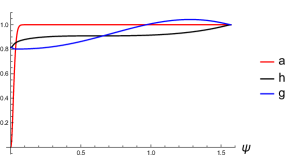
Figure 18: Example of soliton solution with $n=1$ and large $e$. Here we set $e=500$, $m^{2}=-0.9$, $G=0.1$, $\kappa=-1.000$.

From eq. (2.25), we have $H(r)\approx H_{0}\,r$ nearby $r=0$. We expect that $H_{0}$ gets large for $e\to\infty$. Nearby $r=0$, we can approximate the equation for $a$ in eq. (2.15) as follows

$$a^{\prime\prime}=\frac{a^{\prime}}{r}+2e^{2}(a-1)\,H_{0}^{2}r^{2}\,.$$ (C.1)

Imposing that $a$ vanishes at the origin and tends to $1$ outside the central region, we find the solution

$$a=1-\exp\left(-\frac{H_{0}e\,r^{2}}{\sqrt{2}}\right)\,.$$ (C.2)

The contribution to the energy density $\rho$ at the center of the vortex scales as

$$\rho\approx 2H_{0}^{2}\,\exp(-\sqrt{2}\,H_{0}e\,r^{2})\,,$$ (C.3)

which has a rectangular shape, with height $\propto H_{0}^{2}$ and size $\propto\frac{1}{\sqrt{eH_{0}}}$. If $H_{0}$ would scale as $e$ at large $e$, this would give a representation of a $\delta$ function. If instead $H_{0}$ scales slower than $e$, eq. (C.3) tends to zero. By numerical analysis for $G=0.1$ and $\kappa=-1$, we find $H_{0}\propto e^{0.7}$. This suggests that, if we fix $\kappa$ and increase $e$ we do not have a critical $e$ for which the soliton solutions becomes a black hole. This is confirmed by the numerical solution in figure 18.

References

- [1] S. A. Hartnoll, C. P. Herzog and G. T. Horowitz, “Building a Holographic Superconductor,” Phys. Rev. Lett. 101 (2008), 031601 doi:10.1103/PhysRevLett.101.031601 [arXiv:0803.3295 [hep-th]].
- [2] S. A. Hartnoll, C. P. Herzog and G. T. Horowitz, “Holographic Superconductors,” JHEP 12 (2008), 015 doi:10.1088/1126-6708/2008/12/015 [arXiv:0810.1563 [hep-th]].
- [3] S. R. Coleman, “There are no Goldstone bosons in two-dimensions,” Commun. Math. Phys. 31 (1973), 259-264 doi:10.1007/BF01646487
- [4] N. D. Mermin and H. Wagner, “Absence of ferromagnetism or antiferromagnetism in one-dimensional or two-dimensional isotropic Heisenberg models,” Phys. Rev. Lett. 17 (1966), 1133-1136 doi:10.1103/PhysRevLett.17.1133
- [5] P. C. Hohenberg, “Existence of Long-Range Order in One and Two Dimensions,” Phys. Rev. 158 (1967), 383-386 doi:10.1103/PhysRev.158.383
- [6] D. Anninos, S. A. Hartnoll and N. Iqbal, “Holography and the Coleman-Mermin-Wagner theorem,” Phys. Rev. D 82 (2010), 066008 doi:10.1103/PhysRevD.82.066008 [arXiv:1005.1973 [hep-th]].
- [7] K.Yu. Arutyunov, D.S. Golubev, A.D. Zaikin, “Superconductivity in one dimension,”, Physics Reports, Volume 464, Issues 1–2, July 2008, Pages 1-70, doi:10.1016/j.physrep.2008.04.009, arXiv:0805.2118
- [8] C. N. Lau, N. Markovic, M. Bockrath, A. Bezryadin, and M. Tinkham, “Quantum Phase Slips in Superconducting Nanowires”, Physical Review Letters, Volume 87, Number 21, 19 November 2001, doi: 10.1103/PhysRevLett.87.217003
- [9] S. W. Hawking and D. N. Page, “Thermodynamics of Black Holes in anti-De Sitter Space,” Commun. Math. Phys. 87 (1983), 577 doi:10.1007/BF01208266
- [10] E. Witten, “Anti-de Sitter space, thermal phase transition, and confinement in gauge theories,” Adv. Theor. Math. Phys. 2 (1998), 505-532 doi:10.4310/ATMP.1998.v2.n3.a3 [arXiv:hep-th/9803131 [hep-th]].
- [11] G. T. Horowitz and R. C. Myers, “The AdS / CFT correspondence and a new positive energy conjecture for general relativity,” Phys. Rev. D 59 (1998), 026005 doi:10.1103/PhysRevD.59.026005 [arXiv:hep-th/9808079 [hep-th]].
- [12] S. Surya, K. Schleich and D. M. Witt, “Phase transitions for flat AdS black holes,” Phys. Rev. Lett. 86 (2001), 5231-5234 doi:10.1103/PhysRevLett.86.5231 [arXiv:hep-th/0101134 [hep-th]].
- [13] T. Nishioka, S. Ryu and T. Takayanagi, “Holographic Superconductor/Insulator Transition at Zero Temperature,” JHEP 03 (2010), 131 doi:10.1007/JHEP03(2010)131 [arXiv:0911.0962 [hep-th]].
- [14] G. T. Horowitz and B. Way, “Complete Phase Diagrams for a Holographic Superconductor/Insulator System,” JHEP 11 (2010), 011 doi:10.1007/JHEP11(2010)011 [arXiv:1007.3714 [hep-th]].
- [15] E. Witten, “Multitrace operators, boundary conditions, and AdS / CFT correspondence,” [arXiv:hep-th/0112258 [hep-th]].
- [16] M. Berkooz, A. Sever and A. Shomer, “’Double trace’ deformations, boundary conditions and space-time singularities,” JHEP 05 (2002), 034 doi:10.1088/1126-6708/2002/05/034 [arXiv:hep-th/0112264 [hep-th]].
- [17] T. Faulkner, G. T. Horowitz and M. M. Roberts, “Holographic quantum criticality from multi-trace deformations,” JHEP 04 (2011), 051 doi:10.1007/JHEP04(2011)051 [arXiv:1008.1581 [hep-th]].
- [18] K. M. Lee, V. P. Nair and E. J. Weinberg, “Black holes in magnetic monopoles,” Phys. Rev. D 45 (1992), 2751-2761 doi:10.1103/PhysRevD.45.2751 [arXiv:hep-th/9112008 [hep-th]].
- [19] P. Breitenlohner, P. Forgacs and D. Maison, “Gravitating monopole solutions,” Nucl. Phys. B 383 (1992), 357-376 doi:10.1016/0550-3213(92)90682-2
- [20] M. E. Ortiz, “Curved space magnetic monopoles,” Phys. Rev. D 45 (1992), R2586-R2589 doi:10.1103/PhysRevD.45.R2586
- [21] P. Breitenlohner, P. Forgacs and D. Maison, “Gravitating monopole solutions. 2,” Nucl. Phys. B 442 (1995), 126-156 doi:10.1016/S0550-3213(95)00100-X [arXiv:gr-qc/9412039 [gr-qc]].
- [22] A. Lue and E. J. Weinberg, “Magnetic monopoles near the black hole threshold,” Phys. Rev. D 60 (1999), 084025 doi:10.1103/PhysRevD.60.084025 [arXiv:hep-th/9905223 [hep-th]].
- [23] E. J. Weinberg, “Black holes with hair,” NATO Sci. Ser. II 60 (2002), 523-544 doi:10.1007/978-94-010-0347-6_21 [arXiv:gr-qc/0106030 [gr-qc]].
- [24] M. A. Melvin, “Pure magnetic and electric geons,” Phys. Lett. 8 (1964), 65-70 doi:10.1016/0031-9163(64)90801-7
- [25] G. Clement, “Classical solutions in three-dimensional Einstein-Maxwell cosmological gravity,” Class. Quant. Grav. 10 (1993), L49-L54 doi:10.1088/0264-9381/10/5/002
- [26] E. W. Hirschmann and D. L. Welch, “Magnetic solutions to (2+1) gravity,” Phys. Rev. D 53 (1996), 5579-5582 doi:10.1103/PhysRevD.53.5579 [arXiv:hep-th/9510181 [hep-th]].
- [27] M. Cataldo and P. Salgado, “Static Einstein-Maxwell solutions in (2+1)-dimensions,” Phys. Rev. D 54 (1996), 2971-2974 doi:10.1103/PhysRevD.54.2971
- [28] O. J. C. Dias and J. P. S. Lemos, “Rotating magnetic solution in three-dimensional Einstein gravity,” JHEP 01 (2002), 006 doi:10.1088/1126-6708/2002/01/006 [arXiv:hep-th/0201058 [hep-th]].
- [29] M. Banados, C. Teitelboim and J. Zanelli, “The Black hole in three-dimensional space-time,” Phys. Rev. Lett. 69 (1992) 1849 doi:10.1103/PhysRevLett.69.1849 [hep-th/9204099].
- [30] M. Banados, M. Henneaux, C. Teitelboim and J. Zanelli, “Geometry of the (2+1) black hole,” Phys. Rev. D 48 (1993) 1506 Erratum: [Phys. Rev. D 88 (2013) 069902] doi:10.1103/PhysRevD.48.1506, 10.1103/PhysRevD.88.069902 [gr-qc/9302012].
- [31] C. Martinez, C. Teitelboim and J. Zanelli, “Charged rotating black hole in three space-time dimensions,” Phys. Rev. D 61 (2000), 104013 doi:10.1103/PhysRevD.61.104013 [arXiv:hep-th/9912259 [hep-th]].
- [32] M. Montull, O. Pujolas, A. Salvio and P. J. Silva, “Flux Periodicities and Quantum Hair on Holographic Superconductors,” Phys. Rev. Lett. 107 (2011), 181601 doi:10.1103/PhysRevLett.107.181601 [arXiv:1105.5392 [hep-th]].
- [33] M. Montull, O. Pujolas, A. Salvio and P. J. Silva, “Magnetic Response in the Holographic Insulator/Superconductor Transition,” JHEP 04 (2012), 135 doi:10.1007/JHEP04(2012)135 [arXiv:1202.0006 [hep-th]].
- [34] W. A. Little and R. D. Parks, “Observation of Quantum Periodicity in the Transition Temperature of a Superconducting Cylinder”, Physical Review Letters 9, 9 (1962), doi:10.1103/PhysRevLett.9.9
- [35] G. T. Horowitz and M. M. Roberts, “Zero Temperature Limit of Holographic Superconductors,” JHEP 11 (2009), 015 doi:10.1088/1126-6708/2009/11/015 [arXiv:0908.3677 [hep-th]].
- [36] A. A. Abrikosov, “On the Magnetic properties of superconductors of the second group,” Sov. Phys. JETP 5 (1957), 1174-1182
- [37] H. B. Nielsen and P. Olesen, “Vortex Line Models for Dual Strings,” Nucl. Phys. B 61 (1973), 45-61 doi:10.1016/0550-3213(73)90350-7
- [38] A. R. Lugo and F. A. Schaposnik, “Monopole and dyon solutions in AdS space,” Phys. Lett. B 467 (1999), 43-53 doi:10.1016/S0370-2693(99)01178-8 [arXiv:hep-th/9909226 [hep-th]].
- [39] A. R. Lugo, E. F. Moreno and F. A. Schaposnik, “Monopole solutions in AdS space,” Phys. Lett. B 473 (2000), 35-42 doi:10.1016/S0370-2693(99)01481-1 [arXiv:hep-th/9911209 [hep-th]].
- [40] S. Bolognesi and D. Tong, “Monopoles and Holography,” JHEP 01 (2011), 153 doi:10.1007/JHEP01(2011)153 [arXiv:1010.4178 [hep-th]].
- [41] A. Esposito, S. Garcia-Saenz, A. Nicolis and R. Penco, “Conformal solids and holography,” JHEP 12 (2017), 113 doi:10.1007/JHEP12(2017)113 [arXiv:1708.09391 [hep-th]].
- [42] N. Zenoni, R. Auzzi, S. Caggioli, M. Martinelli and G. Nardelli, “A falling magnetic monopole as a holographic local quench,” JHEP 11 (2021), 048 doi:10.1007/JHEP11(2021)048 [arXiv:2106.13757 [hep-th]].
- [43] A. Edery, “Non-singular vortices with positive mass in 2+1 dimensional Einstein gravity with AdS3 and Minkowski background,” JHEP 01 (2021), 166 doi:10.1007/JHEP01(2021)166 [arXiv:2004.09295 [hep-th]].
- [44] J. Albert, “The Abrikosov vortex in curved space,” JHEP 09 (2021), 012 doi:10.1007/JHEP09(2021)012 [arXiv:2106.12260 [hep-th]].
- [45] A. Edery, “Nonminimally coupled gravitating vortex: Phase transition at critical coupling c in AdS3,” Phys. Rev. D 106 (2022) no.6, 065017 doi:10.1103/PhysRevD.106.065017 [arXiv:2205.12175 [hep-th]].
- [46] M. Cadoni, P. Pani and M. Serra, “Scalar hairs and exact vortex solutions in 3D AdS gravity,” JHEP 01 (2010), 091 doi:10.1007/JHEP01(2010)091 [arXiv:0911.3573 [hep-th]].
- [47] L. Y. Hung and A. Sinha, “Holographic quantum liquids in 1+1 dimensions,” JHEP 01 (2010), 114 doi:10.1007/JHEP01(2010)114 [arXiv:0909.3526 [hep-th]].
- [48] J. Ren, “One-dimensional holographic superconductor from AdS3/CFT2 correspondence,” JHEP 11 (2010), 055 doi:10.1007/JHEP11(2010)055 [arXiv:1008.3904 [hep-th]].
- [49] J. Sonner, A. del Campo and W. H. Zurek, “Universal far-from-equilibrium Dynamics of a Holographic Superconductor,” Nature Commun. 6 (2015), 7406 doi:10.1038/ncomms8406 [arXiv:1406.2329 [hep-th]].
- [50] E. Poisson, “A relativist’s toolkit,” Cambridge University Press
- [51] P. Breitenlohner and D. Z. Freedman, “Stability in Gauged Extended Supergravity,” Annals Phys. 144 (1982), 249 doi:10.1016/0003-4916(82)90116-6
- [52] Ó. J. C. Dias, G. T. Horowitz, N. Iqbal and J. E. Santos, “Vortices in holographic superfluids and superconductors as conformal defects,” JHEP 04 (2014), 096 doi:10.1007/JHEP04(2014)096 [arXiv:1311.3673 [hep-th]].
- [53] D. Marolf and S. F. Ross, “Boundary Conditions and New Dualities: Vector Fields in AdS/CFT,” JHEP 11 (2006), 085 doi:10.1088/1126-6708/2006/11/085 [arXiv:hep-th/0606113 [hep-th]].
- [54] E. Witten, “SL(2,Z) action on three-dimensional conformal field theories with Abelian symmetry,” [arXiv:hep-th/0307041 [hep-th]].
- [55] O. Domenech, M. Montull, A. Pomarol, A. Salvio and P. J. Silva, “Emergent Gauge Fields in Holographic Superconductors,” JHEP 08 (2010), 033 doi:10.1007/JHEP08(2010)033 [arXiv:1005.1776 [hep-th]].
- [56] K. Jensen, “Chiral anomalies and AdS/CMT in two dimensions,” JHEP 01 (2011), 109 doi:10.1007/JHEP01(2011)109 [arXiv:1012.4831 [hep-th]].
- [57] T. Faulkner and N. Iqbal, “Friedel oscillations and horizon charge in 1D holographic liquids,” JHEP 07 (2013), 060 doi:10.1007/JHEP07(2013)060 [arXiv:1207.4208 [hep-th]].
- [58] R. Argurio, G. Giribet, A. Marzolla, D. Naegels and J. A. Sierra-Garcia, “Holographic Ward identities for symmetry breaking in two dimensions,” JHEP 04 (2017), 007 doi:10.1007/JHEP04(2017)007 [arXiv:1612.00771 [hep-th]].
- [59] V. Balasubramanian and P. Kraus, “A Stress tensor for Anti-de Sitter gravity,” Commun. Math. Phys. 208 (1999), 413-428 doi:10.1007/s002200050764 [arXiv:hep-th/9902121 [hep-th]].
- [60] K. Skenderis, “Lecture notes on holographic renormalization,” Class. Quant. Grav. 19 (2002), 5849-5876 doi:10.1088/0264-9381/19/22/306 [arXiv:hep-th/0209067 [hep-th]].
- [61] M. Henningson and K. Skenderis, “The Holographic Weyl anomaly,” JHEP 07 (1998), 023 doi:10.1088/1126-6708/1998/07/023 [arXiv:hep-th/9806087 [hep-th]].
- [62] I. Papadimitriou, “Multi-Trace Deformations in AdS/CFT: Exploring the Vacuum Structure of the Deformed CFT,” JHEP 05 (2007), 075 doi:10.1088/1126-6708/2007/05/075 [arXiv:hep-th/0703152 [hep-th]].
- [63] M. M. Caldarelli, A. Christodoulou, I. Papadimitriou and K. Skenderis, “Phases of planar AdS black holes with axionic charge,” JHEP 04 (2017), 001 doi:10.1007/JHEP04(2017)001 [arXiv:1612.07214 [hep-th]].
- [64] M. Astorino, “Charging axisymmetric space-times with cosmological constant,” JHEP 06 (2012), 086 doi:10.1007/JHEP06(2012)086 [arXiv:1205.6998 [gr-qc]].
- [65] Y. K. Lim, “Electric or magnetic universe with a cosmological constant,” Phys. Rev. D 98 (2018) no.8, 084022 doi:10.1103/PhysRevD.98.084022 [arXiv:1807.07199 [gr-qc]].
- [66] D. Kastor and J. Traschen, “Geometry of AdS-Melvin Spacetimes,” Class. Quant. Grav. 38 (2021) no.4, 045016 doi:10.1088/1361-6382/abd141 [arXiv:2009.14771 [hep-th]].
- [67] A. Anabalon and S. F. Ross, “Supersymmetric solitons and a degeneracy of solutions in AdS/CFT,” JHEP 07 (2021), 015 doi:10.1007/JHEP07(2021)015 [arXiv:2104.14572 [hep-th]].
- [68] A. Anabalón, A. Gallerati, S. Ross and M. Trigiante, “Supersymmetric solitons in gauged = 8 supergravity,” JHEP 02 (2023), 055 doi:10.1007/JHEP02(2023)055 [arXiv:2210.06319 [hep-th]].
- [69] O. Aharony, S. S. Gubser, J. M. Maldacena, H. Ooguri and Y. Oz, “Large N field theories, string theory and gravity,” Phys. Rept. 323 (2000), 183-386 doi:10.1016/S0370-1573(99)00083-6 [arXiv:hep-th/9905111 [hep-th]].
- [70] M. Eune, W. Kim and S. H. Yi, “Hawking-Page phase transition in BTZ black hole revisited,” JHEP 03 (2013), 020 doi:10.1007/JHEP03(2013)020 [arXiv:1301.0395 [gr-qc]].
- [71] V. Vakaryuk, “Universal Mechanism for Breaking the hc/2e Periodicity of Flux-Induced Oscillations in Small Superconducting Rings,” Phys.Rev.Lett. 101, 167002 (2008).
- [72] F. Loder et al., “Magnetic flux periodicity of h/e in superconducting loops,” Nat.Phys. 4, 112 (2008).
- [73] T.C. Wei, P.M. Goldbart, “Emergence of h/e-period oscillations in the critical temperature of small superconducting rings threaded by magnetic flux,” Phys.Rev.B77, 224512(2008).
- [74] J. D. Bekenstein, “Nonexistence of baryon number for static black holes,” Phys. Rev. D 5 (1972), 1239-1246 doi:10.1103/PhysRevD.5.1239