The Chinese pulsar timing array data release I

We present polarization pulse profiles for 56 millisecond pulsars (MSPs) monitored by the Chinese Pulsar Timing Array (CPTA) collaboration using the Five-hundred-meter Aperture Spherical radio Telescope (FAST). The observations centered at 1.25 GHz with a raw bandwidth of 500 MHz. Due to the high sensitivity ($\sim$16 K/Jy) of the FAST telescope and our long integration time, the high signal-to-noise ratio polarization profiles show features hardly detected before. Among 56 pulsars, the polarization profiles of PSRs J0406$+$3039, J1327$+$3423, and J2022$+$2534 were not previously reported. 80% of MSPs in the sample show weak components below 3% of peak flux, 25% of pulsars show interpulse-like structures, and most pulsars show linear polarization position angle jumps. Six pulsars seem to be emitting for full rotation phase, with another thirteen pulsars being good candidates for such a 360^∘ radiator. We find that the distribution of the polarization percentage in our sample is compatible with the normal pulsar distribution. Our detailed evaluation of the MSP polarization properties suggests that the wave propagation effects in the pulsar magnetosphere are important in shaping the MSP polarization pulse profiles.

1 Introduction

Unlike normal pulsars, millisecond pulsars (MSPs) have significantly shorter spin periods and lower values of period derivatives. Some MSPs can work as precise cosmic clocks comparable to atomic clocks in stability (Taylor 1991; Hobbs et al. 2012; Verbiest & Shaifullah 2018; Hobbs et al. 2020). With the high timing precision, some MSPs have been utilized to form the pulsar timing array (PTA; Foster & Backer 1990) in order to search for nanohertz gravitational waves (GWs; Sazhin 1978; Detweiler 1979). Recently, several PTAs have presented evidence of nanohertz GW signals (Agazie et al. 2023; EPTA Collaboration et al. 2023; Reardon et al. 2023; Xu et al. 2023). To facilitate the detection of GWs, MSPs are monitored regularly for long time spans, producing extensive datasets. The obtained polarization profiles have high signal-to-noise ratios (S/Ns). Such a high-S/N dataset is beneficial to study the emission properties of MSPs, since the delicate structures and very weak components can be detected. On the other hand, long-term observation activities can provide valuable insights into the stability of MSP profiles (Xu et al. 2021), allowing for the study of the dynamic evolution of MSP magnetospheres. In addition, a careful polarization calibration procedure is necessary to minimize the instrumental effects on pulsar timing. Through a comparison with the polarization profiles of previous studies, we can perform cross-validation on the calibration and data processing procedures.

Both MSPs and normal pulsars show similar profile complexity (Kramer et al. 1998), spectral indexes, and polarization properties (Kramer et al. 1999; Yan et al. 2011; Dai et al. 2015; Gentile et al. 2018; Spiewak et al. 2022; Wahl et al. 2022; Gitika et al. 2023; Karastergiou et al. 2024). Furthermore, MSPs exhibit similar polarization profile characteristics compared to normal pulsars, which includes linear and circular polarization components, linear polarization angle swing, interpulse, orthogonal polarization mode jumps (OPMs), and sense reversal of circular polarization (Thorsett 1991; Xilouris et al. 1998; Manchester & Han 2004). These observational facts indicate that the radiation mechanisms are same for MSPs and normal pulsars.

On the other hand, the light cylinder ($R_{\rm LC}=P_{0}c/2\pi$), where the co-rotation velocity is equal to the light speed, is of smaller radii for MSPs by a factor of 10 to 1000 compared to normal pulsars. Consequently, the size of MSP magnetosphere is much smaller. It will inevitably affect the radiation geometry and propagation of radio waves in the magnetosphere (Jones 2020). In fact, observations had shown that some polarization properties of MSPs differ significantly from those of normal pulsars. As was expected geometrically (Komesaroff 1970), MSPs have much larger duty cycles and pulse widths. Unlike for normal pulsars, the profile widths and separations between pulse components in MSPs remain nearly constant across frequencies, illustrating more compact emission regions (Kramer et al. 1999; Dai et al. 2015). In addition, a large portion of MSPs contain interpulse in their profiles, which is in contrast to the normal pulsar population (Thorsett 1991; Manchester & Han 2004; Yan et al. 2011). The PA slopes of MSPs are much shallower. Moreover, the linear polarization position angle (PA) curves of most MSPs deviate from the rotating vector model (RVM; Radhakrishnan & Cooke 1969; Komesaroff 1970; Xilouris et al. 1998; Manchester & Han 2004; Wahl et al. 2022), which is generally applicable for normal pulsars(Johnston et al. 2023). The irregular PA curves indicate a much more complex (non-dipolar) magnetic filed structure in MSPs (Chung & Melatos 2011). These differences indicate that the magnetospheres of MSPs are not simply a scaled-down version of that in normal pulsars.

To understand the radiation mechanism and magnetosphere of MSPs better, qualitative polarization measurements of MSPs are essential. Polarization properties of normal pulsars have been extensively studied (e.g., see Johnston & Kerr (2018); Wang et al. (2023)). In this paper, we focus on the polarization studies for MSPs. High-quality polarization profiles for 56 MSPs are presented here. The data is from the Chinese Pulsar Timing Array (CPTA; Lee 2016) observation carried out at FAST (Jiang et al. 2019). The large sample size and high-S/N data allow for a detailed investigation of the polarization properties of MSPs. In Sect. 2, we describe the observation activities. The detailed calibration pipeline and data processing are explained in Sect. 3. In Sects. 4 and 5, we summarize and discuss the properties of MSP polarization. The conclusions are made in Sect. 6.

2 Observations

We analyzed data for 56 pulsars from the first data release of CPTA (Xu et al. 2023). PSR J0218$+$4232 was excluded from the polarization studies of this paper, because it shows radiation at all rotation phases and the baseline of pulse profile cannot be uniquely determined. Moreover, the profile presents obvious evolution across different orbital phases. Studies of PSR J0218$+$4232 will be published elsewhere. Although PSR J1327$+$3423 is a partially recycled pulsar (Fiore et al. 2023) rather than a canonical MSP, we included it in the CPTA pulsar list due to its high timing precision and timing stability.

Our data were collected using the central beam of the 19-beam receiver (Dunning et al. 2017). The sky coverage of FAST is from $-14^{\circ}$ to 66^∘ on declination. The sensitivity and system noise temperature stay constant at $\sim$ 16 K/Jy and $\sim$ 19 K, respectively, for the central beam within a zenith angle of 26.4^∘ (Jiang et al. 2020). When the zenith angle of the target is larger than 26.4^∘, a back illumination strategy is conducted to avoid ground emission (Jin et al. 2013). In this case, the telescope gain and system noise temperature deteriorate to 11.5 K/Jy and 27 K, when the zenith angle reaches the maximum of 40^∘ (Jiang et al. 2020). We compare the difference in polarimetry for small and large zenith angles in Appendix A. It induces a difference of less than 0.2% in polarization profiles. The effect can thus be safely neglected for most of the application. Nonetheless, the polarization pulse profiles in this paper are mainly from data collected under small zenith angles (¡26.4^∘). For about one quarter of the 56 pulsars, we only observed with back illumination mode; that is, for PSR J0034$-$0534, J0613$-$0200, J1012$+$5307, J1024$-$0719, J1643$-$1224, J1744$-$1134, J1832$-$0836, J1843$-$1113, J1911$-$1114, J1918$-$0642, J2010$-$1323, J2145$-$0750, and J2150$-$0326.

The observation cadence for all pulsars is approximately once per two weeks, determined by the amount of FAST observing time allocated for the CPTA project. One exception is PSR J1713$+$0747, which was observed weekly due to its high timing precision. The digital backend at FAST saves data in the filterbank format; that is, it records the signal power as a function of frequency and time. The observation covers the frequency range of 1-1.5 GHz with a spectral resolution of 122.07 kHz and takes a time resolution of 49.152 $\mu$s. We dedispersed and folded the filterbank data using DSPSR (van Straten & Bailes 2011) to form 20-minute sub-integration pulsar data. For pulsars in compact binaries, the length of sub-integration time was reduced. The total observing time and number of observation epochs for all pulsars are listed in Table 2. More details of our data collection scheme will be explained by Xu et al. 2024 (in prep.).

For each observation, we also recorded periodic on-off noise diode signal for the polarization calibration purposes. Before March 2021, we recorded one-to-two-minute noise signals with periods of 1 or 2 second(s) before or after each observation. After that, we changed the noise injection scheme and the noise was injected to cover the entire observation time span. We note that it can help correct the drift of the electronic system on timescales shorter than 20 minutes. For most pulsars, the pulsar signal will not be affected by this scheme and we can separate the noise calibrator signal from the pulsar signal, thanks to three reasons: 1) the noise level is a factor of 20 lower than the system noise; 2) the noise period does not align with the pulsar period; 3) the noise signal has no dispersion. For certain low dispersion measure (DM) pulsars, such as PSR J1327$+$3423, the noise diode signal cannot be well separated from the pulsar signal, but it has a negligible effect due to the first reason mentioned above.

3 Data analysis

3.1 Polarization calibration

The polarization is described by the Stokes parameters,

$$\mathcal{S}=\left[\begin{array}[]{c}I\\ Q\\ U\\ V\end{array}\right]\,,$$ (1)

where $I$ is the intensity flux, $Q$ and $U$ denote the linear polarization, and $V$ is the circular polarization. Here, we take the PSR/IEEE convention where the left circular polarization is positive (van Straten et al. 2010). Based on the Stokes parameter, we can define the linear polarization position angle ($\Psi$) and the ellipticity angle ($\chi$) as

$$\tan 2\Psi=\frac{U}{Q}\,,$$ (2)

$$\sin 2\chi=\frac{V}{\sqrt{Q^{2}+U^{2}+V^{2}}}\,.$$

The imperfectness of receiver will contaminate the polarization measurements. In order to obtain the intrinsic Stokes parameters, corrections for the instrumental effects are necessary. All the linear effects affecting Stokes parameters can be empirically expressed as  (Lorimer & Kramer 2012),

$$\mathcal{S}_{\mathrm{obs}}=\mathcal{M}_{\mathrm{Amp}}\times\mathcal{M}_{\mathrm{CC}}\times\mathcal{M}_{\mathrm{PA}}\times\mathcal{S}_{\mathrm{int}}\,,$$ (3)

which means that the intrinsic polarization ($\mathcal{S}_{\mathrm{int}}$) is firstly affected by effects described by the Müller matrix, $\mathcal{M}_{\mathrm{PA}}$, then $\mathcal{M}_{\mathrm{CC}}$ and $\mathcal{M}_{\mathrm{Amp}}$.

The first effect, represented by the Müller matrix, $\mathcal{M}_{\mathrm{PA}}$, is caused by feed rotation, which induces a parallactic angle between the feed orientation and the plane of polarization. For FAST, we do not need to perform such a correction, since it is corrected by mechanically rotating the 19-beam receiver (Jiang et al. 2020) such that one feed always aligns with the northern direction.

The second effect, $\mathcal{M}_{\mathrm{CC}}$, comes from polarization leakage caused by the cross-coupling between the x and y feeds, such as the non-orthogonality of the instrument polarization basis. It has been shown that such leakage for the central beam of the 19-beam feed is only at a level of $\sim$ 0.034 $\%$ (Ching et al. 2022). Since such an effect is negligible for the current work, we leave it for future work.

The third effect, $\mathcal{M}_{\mathrm{Amp}}$, is from the differential gain and phase imbalance. In general, the electric signals of the two polarization feeds pass through two separate signal chains with different amplifiers. There will inevitably be differences in time delays and amplifier gains between the two signal chains. Such an effect is described by the following Müller matrix (Heiles et al. 2001b):

$$\mathcal{M}_{\text{Amp }}=\left[\begin{array}[]{cccc}1&\Delta G/2&0&0\\ \Delta G/2&1&0&0\\ 0&0&\cos\Delta\phi&-\sin\Delta\phi\\ 0&0&\sin\Delta\phi&\cos\Delta\phi\end{array}\right]\,,$$ (4)

where $\Delta G$ and $\Delta\phi$ are the differential gain and phase, respectively.

As the leakage term can be neglected, we adopted the single axis model for polarization calibration using the noise signal equally injected into the two feeds (Hotan et al. 2004), where the two feeds see the noise as of the same amplitude and phase. As an example, the derived Müller matrix elements at different epochs and frequencies through the package PSRCHIVE (Hotan et al. 2004) are shown in Fig. 1 . We note that the differential gain of the system fluctuates by approximately 20%, while the differential phase after July 2020 (MJD 59059) is stable up to only a few degrees. One can also see that the $\Delta G$ and $\Delta\phi$ change more rapidly as functions of frequency at the band edges; that is, for frequencies close to 1000 MHz or 1500 MHz. Here, the feed loses sensitivity and has a poor response. Therefore, we removed the 20 MHz band edge on each side of the band pass to obtain reliable polarization data for the subsequent analysis.

Since all pulsar observations are accompanied by calibration observations, we applied the calibration solution to the corresponding pulsar observations for correction of instrumental effects through PSRCHIVE (Hotan et al. 2004). The next step was to correct the Faraday rotation effects induced by the interstellar medium (ISM) and Galactic magnetic fields.

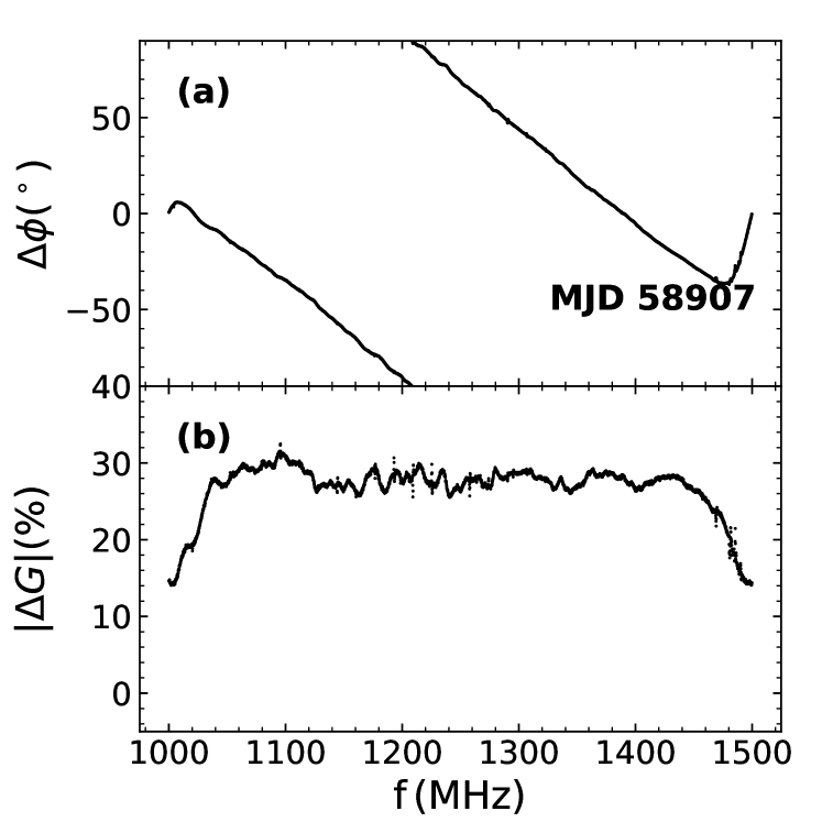
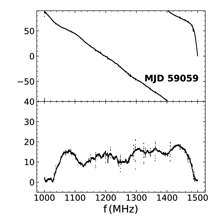
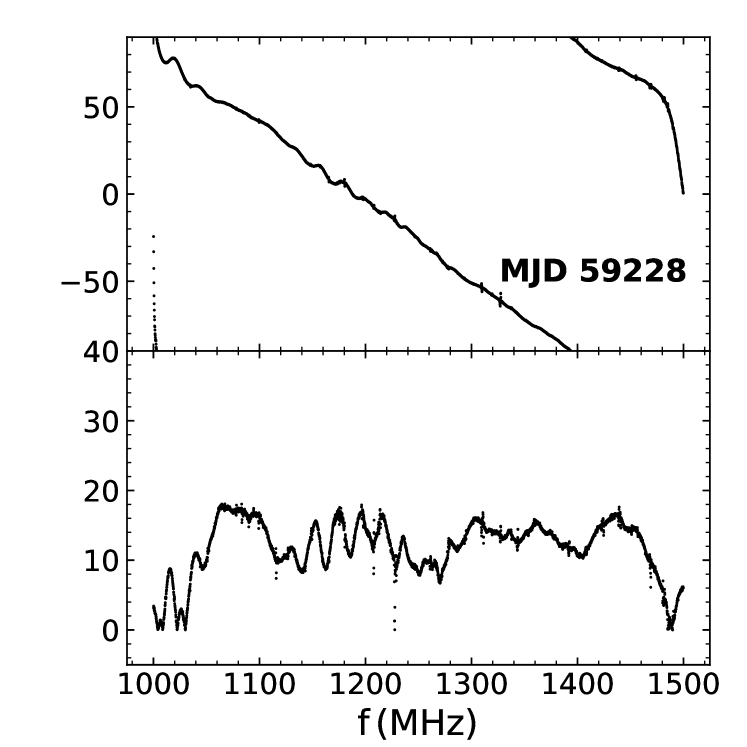
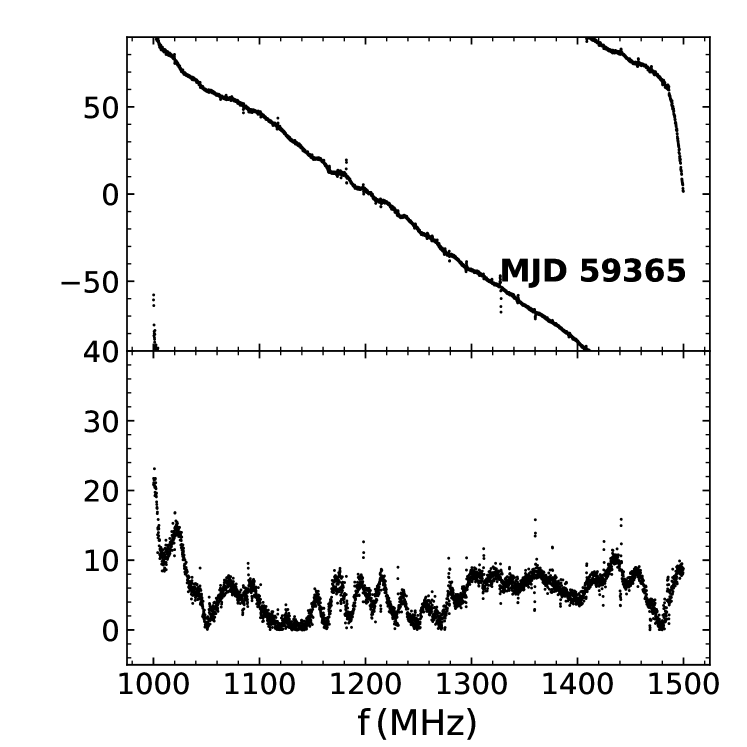
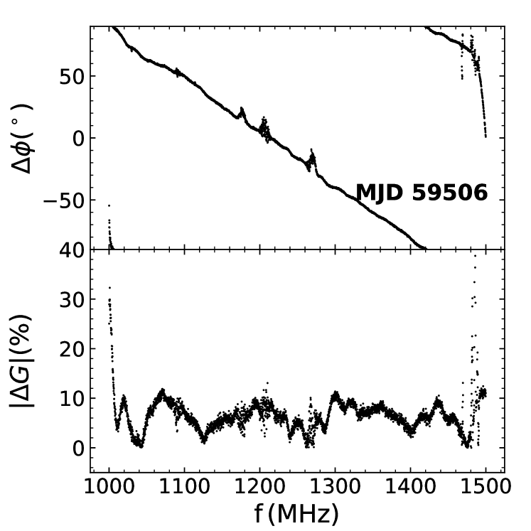
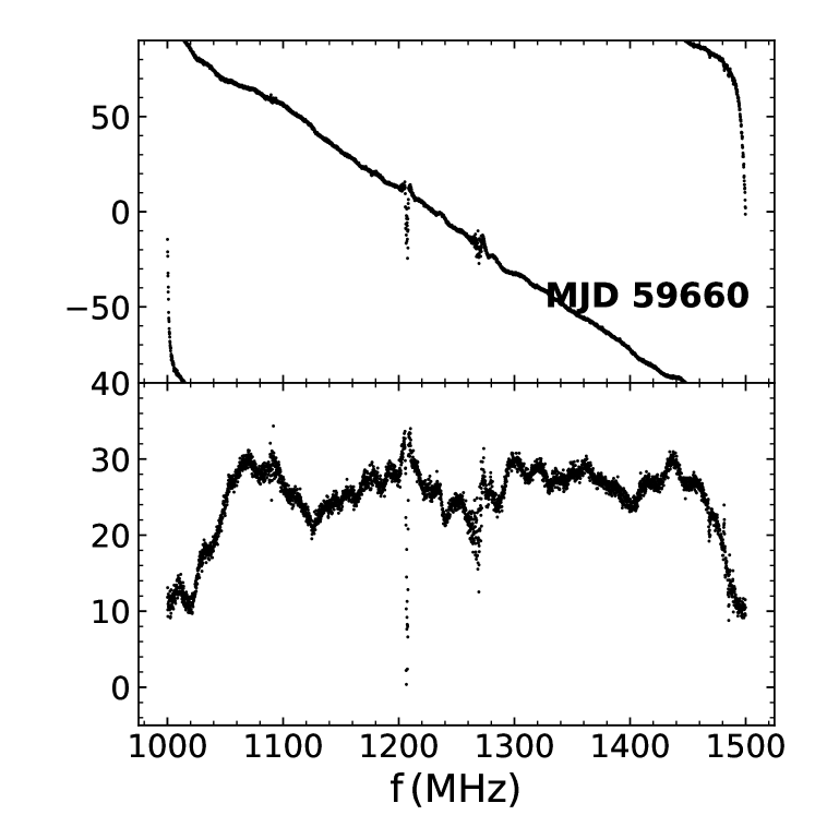
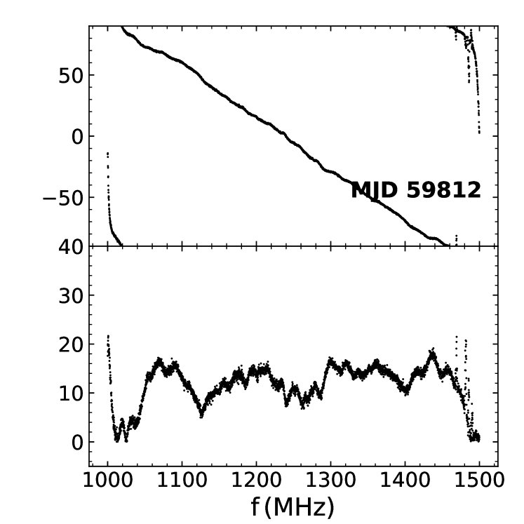
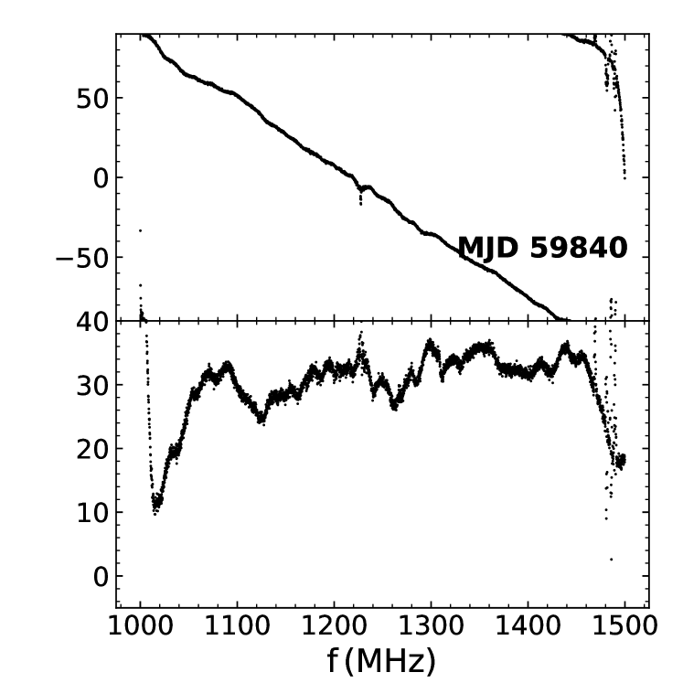
Figure 1: Differential gains and phases as functions of observing frequencies at eight epochs for PSR J0023$+$0923. The differential phase and gains between the two amplifier chains are shown in panels (a) and (b), respectively.

3.2 Faraday rotation correction

When the radio waves propagate through the magnetoionized ISM, the linear polarization PA rotates by $\Delta\Psi(\lambda)={\rm RM}\lambda^{2}$, where $\lambda$ is the wavelength of radio wave and RM is the integral of parallel magnetic field strength and electron density along the line of sight:

$${\rm RM}=\frac{e^{3}}{2\pi m_{e}^{2}c^{4}}\int_{0}^{d}n_{e}(l)B_{\|}(l)dl\,,$$ (5)

where $d$ is the distance from the pulsar to the earth, $n_{e}$ is the free electron density, and $B_{\|}$ is the magnetic field strength projected to the line of sight. Constants $e$, $m_{\rm e}$, and $c$ are electron charge, mass, and light speed, respectively.

We used two different methods to measure the RM for cross-checking. The first method derived the RM value through fitting the profiles of Stokes $Q$ and $U$ across frequencies (van Straten et al. 2012; Desvignes et al. 2019), where the nested sampling package MULTINEST (Feroz et al. 2009) was used to infer the model parameters. The second method was the generalized RM synthesis, which searches across a range of RMs to “de-rotate” the wrapped linear polarization. The best RM was found by maximizing the total linear polarization given by (Brentjens, M. A. & de Bruyn, A. G. 2005; Schnitzeler & Lee 2015),

$${\rm\bf p}(\rm RM)=\int^{\nu_{\rm high}}_{\nu_{\rm low}}{{\rm\bf L}(\nu)}{\rm\bf v}({\rm RM},\nu)d\nu\,,$$ (6)

where $\nu$ is the frequency, and ${\rm\bf L}(\nu)$ is the complex linear polarization spectrum in the frequency range of $\nu_{\rm low}$ to $\nu_{\rm high}$, defined as ${\rm\bf L}(\nu)=Q(\nu)+iU(\nu)$. The de-rotation vector, ${\rm\bf v}({\rm RM},\nu)$, is defined in Schnitzeler & Lee (2015). The differences between the RM values derived from the Bayesian $Q$-$U$ fitting and the generalized RM synthesis methods are negligible (see Appendix B). In the following parts of the paper, we quote RM values from the $Q$-$U$ fitting method.

It is necessary to clarify that, for each of the above two methods, there are two ways to perform the data analysis. One uses the phase-integrated Stokes $Q$ and $U$ at each frequency, and the other one firstly derives the RM at each phase bin and then performs averaging along the phase. The former way is less sensitive to the noise due to the phase integration, but it will be affected by the depolarization due to intrinsic PA swing in pulse profiles. The latter one avoids the depolarization effect, but it is more susceptible to noise. Since MSPs generally present violent PA swings and illusive RM evolution across the pulse phase (see Ilie et al. (2018); Dai et al. (2015) and later discussion), we used the second method to estimate the RM.

Step (1): We computed the Faraday spectra for each phase bin to avoid the depolarization effect and summed them up to give a preliminary RM value for each observation.

Step (2): We corrected the Faraday rotation effect and produced the integrated polarization profile by summing up all observations. In this process, observations with a maximal phase-resolved S/N lower than 50 were discarded. In practice, the fractions of discarded observations are much less than 10 $\%$. In order to further reduce effects from violent PA variations, the final PA curves were sliced into intervals of $10^{\circ}$, which were then used to divide pulse phases for each observation. An example of such phase division is shown in Fig. 2 .

Step (3): After the data were sliced into many phase segments, the corresponding RM value of each phase segment was derived separately through the $Q$-$U$ fitting method. We adopted the weighted average as the final RM value for each observation, where the statistical uncertainty of RM in each interval was taken as the weight. Outliers with differences larger than $30\,\mathrm{rad\cdot m^{-2}}$ were removed in the averaging process.

Step (4): After correcting the Faraday rotation for all observations, the integrated profiles and averaged RM values were obtained for each pulsar. In order to check whether residual RM exists in the final profiles, we computed the phase-resolved RM by applying the $Q$-$U$ fitting to the data. For most pulsars, we detected few residual RM variations across the pulse phase. Some pulsars, however, show significant residual RM variation across the pulse phase, as is shown in Fig. 3 . Such phase-resolved RM variation is likely to be illusive, as we shall discuss in Sect. 5.4.

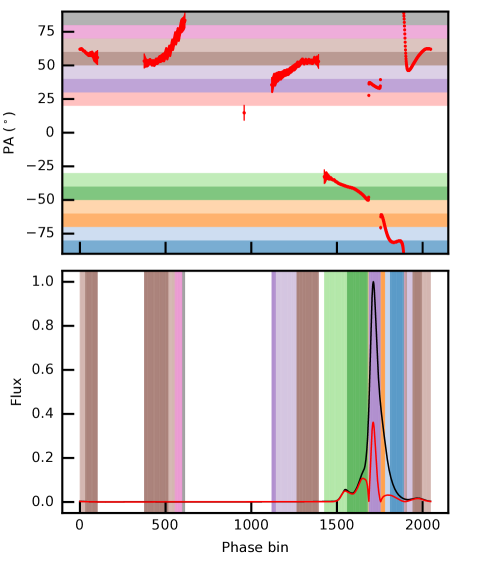
Figure 2: Illustration for the pulse phases slicing scheme for the RM measurement. Upper panel: PA curve and the uniform interval in PA. Bottom panel: Corresponding phase interval determined by the PA interval, marked with the same color as the upper panel. The solid black and red curves are the total intensity and linear polarization of pulse profile, respectively.

We also checked our RM values (after correcting the Earth magnetosphere contribution) with previously published results (Gentile et al. 2018; Wahl et al. 2022; Spiewak et al. 2022; Wang et al. 2023). Our results are compatible with the published values. Here, the software package ionFR (Sotomayor-Beltran et al. 2013) was used to compute the ionospheric corrections, where we used total electron content CODE maps provided by GPS monitoring and interpolated to the observing epoch. The Earth magnetic field model we used is the 13th generation release of the International Geomagnetic Reference Field (Alken et al. 2021).

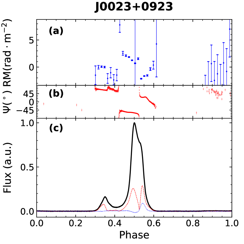
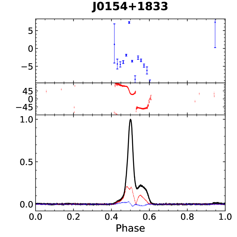
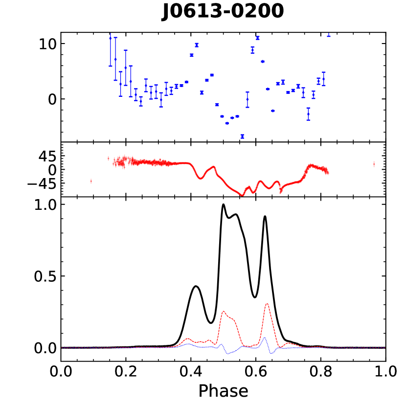
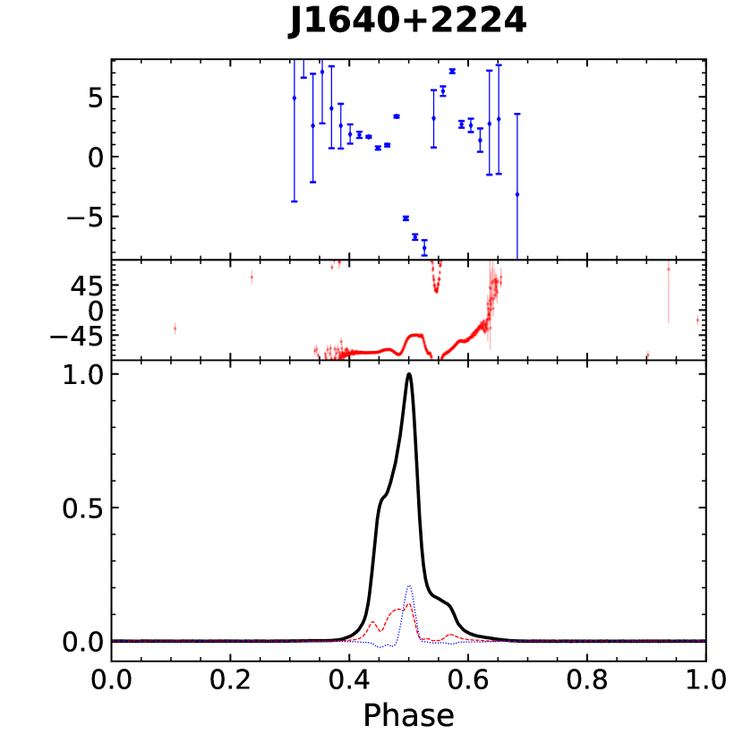
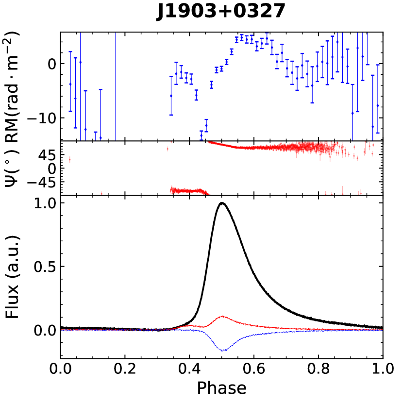
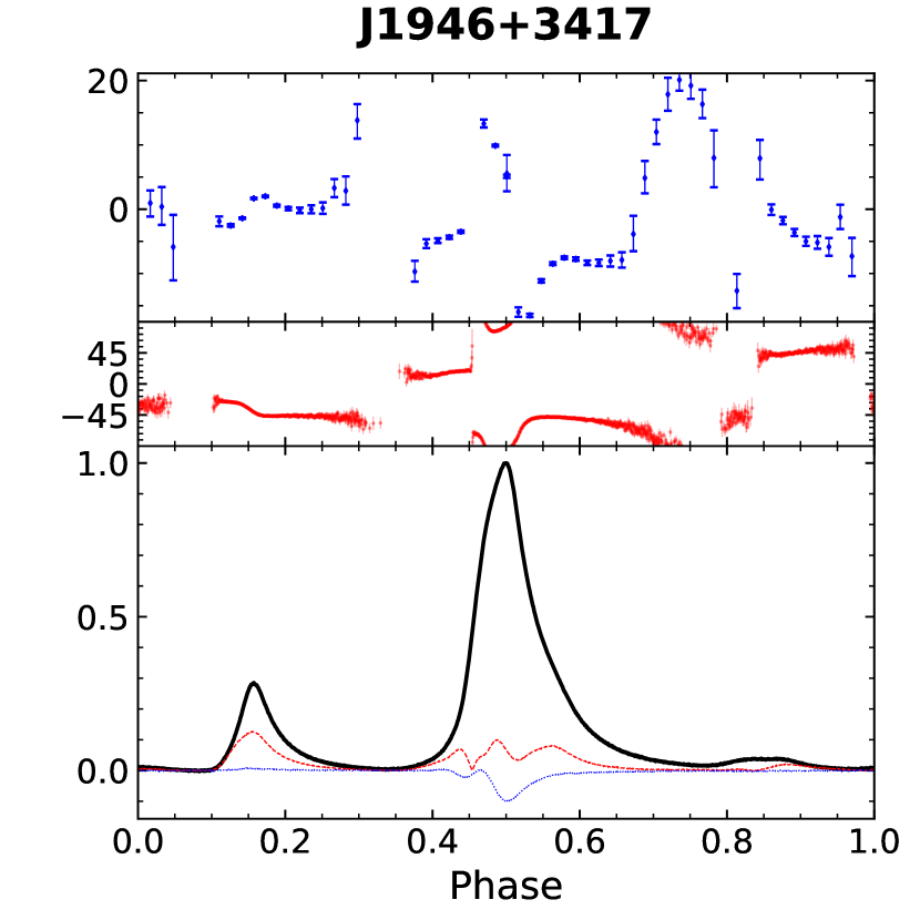
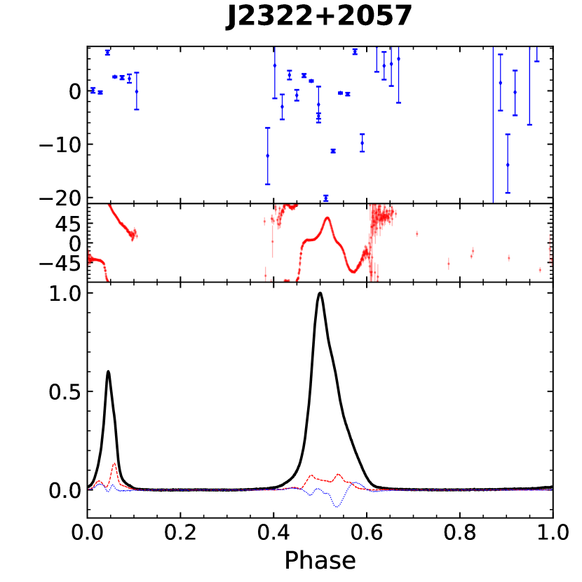
Figure 3: Apparent RM variations along pulse phase detected for eight pulsars. Panel (a) displays the RM variations after subtracting the average RM value. Panel (b) PA curves. Panel (c) polarization pulse profiles, where solid black, dashed red, and dotted blue curves denote the total intensity, linear intensity, and circular polarization intensity, respectively. The profiles were normalized by the maximal intensity and the phase of the intensity peak was set at 0.5.

3.3 Weisberg correction

The linear ($L$) and total polarization ($P$) intensities are defined with the Stokes parameters:

$$L = \sqrt{Q^{2}+U^{2}}\,,$$ (7)

$$P = \sqrt{Q^{2}+U^{2}+V^{2}}\,.$$ (8)

The $L$ and $P$ are always positive, and thus suffer from the statistical bias that their expected values are shifted due to the variance of $Q,U$, and $V$. To correct the bias, we performed the Weisberg correction (see Everett & Weisberg (2001) for the references therein and also the generalized version by Jiang et al. (2022)); that is, $L$ and $P$ were computed with

$$L=\begin{cases}&\sqrt{L^{2}-\frac{\sum_{i,j=1,i\neq j}^{2}S_{i}^{2}\sigma_{S_{j}}^{2}}{L^{2}}},\,\forall L\geq 3\,\sigma_{L}\,,\\ &L,\,\textrm{otherwise}\\ \end{cases}$$ (9)

$$P=\begin{cases}&\sqrt{P^{2}-\frac{\sum_{i,j=1,i\neq j}^{3}S_{i}^{2}\sigma_{S_{j}}^{2}}{P^{2}}},\,\forall P\geq 3\,\sigma_{P}\,,\\ &P,\,\textrm{otherwise}\\ \end{cases}$$

where $S_{i}$ are the Stokes parameters and $S_{1}=Q$, $S_{2}=U$, and $S_{3}=V$. $\sigma_{L}$ and $\sigma_{P}$ are the corresponding baseline noise. We chose the threshold of 3-$\sigma$ to be compatible with later analysis.

4 Results

The final polarization profiles of CPTA pulsars are present online. To the authors’ knowledge, the polarization profiles of three recently discovered pulsars – namely, PSRs J0406$+$3039 (McEwen et al. 2024), J1327$+$3423 (Fiore et al. 2023), and J2022$+$2534 (Swiggum et al. 2023) in the L band (1-2 GHz) – are shown for the first time. We computed the degrees of linear, circular, total polarized, and pulse width for each pulsar, which is summarized in Table 1. CPTA MSPs generally possess a moderate degree of linear polarization and a low circular polarization degree. Seven pulsars have a total fractional polarization higher than 50$\%$, where PSR J1744$-$1134 has the highest total polarization degree ($\sim 90\%$) and PSR J1327$+$3423 features the highest circular polarization of $\sim 27\%$.

No correlation is found between the degree of polarization and the pulsar period, period derivative, and pulse width. Within them, the period and $|V|/I$ show the strongest correlation of 0.45 with the p value of $4.81\times 10^{-4}$. However, with three long-period (¿10 ms) pulsars excluded (PSRs J0621$+$1002, J1327$+$3423, and J2145$-$0750), the coefficient is reduced to 0.19. It is possible that the polarization properties of MSPs are independent of pulsar rotation parameters, or we are limited by the size of our MSP samples.

Table 1: Pulse width and polarization degree of CPTA pulsars. The total, linear, circular, and absolute circular degree of polarization are $\Pi_{\rm P}\equiv\frac{\langle P\rangle}{\langle I\rangle}$, $\Pi_{\rm L}\equiv\frac{\langle L\rangle}{\langle I\rangle}$, $\Pi_{\rm V}\equiv\frac{\langle V\rangle}{\langle I\rangle}$, and $\Pi_{\rm|V|}\equiv\frac{\langle|V|\rangle}{\langle I\rangle}$, where the phase average is denoted with $\langle\rangle$. The detectable pulse width and the effective width are $W_{\rm det}$ and $W_{\rm eff}$, respectively.

Pulsar	$W_{\rm det}$	$W_{\rm eff}$	$\Pi_{\rm P}$	$\Pi_{\rm L}$	$\Pi_{\rm V}$	$\Pi_{\rm|V|}$
	%	%	%	%	%	%
J0023$+$0923	40.1	7.8	30.6	30.0	3.3	4.4
J0030$+$0451	82.1	14.3	33.4	33.1	0.8	3.1
J0034$-$0534	71.9	25.5	17.9	9.4	-12.1	12.1
J0154$+$1833	22.6	5.2	32.2	31.8	0.7	4.1
J0340$+$4130	81.2	9.3	19.4	18.9	-2.5	2.9
J0406$+$3039	57.5	10.3	33.9	32.0	-5.4	8.8
J0509$+$0856	96.7	28.2	35.3	34.0	1.6	4.5
J0605$+$3757	45.0	9.6	46.5	46.6	-0.3	0.4
J0613$-$0200	66.5	16.6	19.9	19.6	0.6	3.1
J0621$+$1002	57.4	5.1	28.1	21.3	-16.2	16.3
J0636$+$5128	28.2	5.6	40.3	38.1	-2.2	6.3
J0645$+$5158	38.7	2.4	22.0	20.0	0.9	6.7
J0732$+$2314	82.3	28.6	33.2	23.6	17.5	21.1
J0751$+$1807	82.3	11.2	30.5	27.3	-9.3	11.6
J0824$+$0028	66.8	13.5	47.6	45.1	6.5	11.3
J1012$+$5307	94.2	15.7	59.2	58.6	0.1	6.6
J1024$-$0719	86.3	13.0	62.4	61.9	1.0	3.6
J1327$+$3423	18.7	2.6	44.2	30.5	27.2	27.6
J1453$+$1902	86.2	9.1	62.9	62.7	-1.7	2.9
J1630$+$3734	79.5	11.8	41.3	39.8	0.1	4.3
J1640$+$2224	36.0	7.0	16.6	12.9	4.4	8.5
J1643$-$1224	79.2	10.2	22.5	17.1	-2.6	12.1
J1710$+$4923	94.7	16.5	19.2	15.4	-1.1	7.5
J1713$+$0747	91.8	4.3	31.7	31.1	-1.6	3.0
J1738$+$0333	41.6	6.5	25.2	24.7	-1.8	3.9
J1741$+$1351	41.4	4.1	21.7	20.9	2.5	4.3
J1744$-$1134	47.0	4.1	88.8	88.8	-1.9	1.9
J1745$+$1017	75.5	12.7	53.9	51.8	-9.7	10.1
J1832$-$0836	71.4	10.2	29.9	27.2	-2.3	7.4
J1843$-$1113	49.3	6.4	37.5	36.8	-0.7	2.2
J1853$+$1303	58.8	11.4	33.6	26.2	3.5	16.9
J1857$+$0943	75.2	12.5	15.3	14.2	-0.1	4.3
J1903$+$0327	83.0	17.5	15.2	9.7	-10.8	10.8
J1910$+$1256	32.8	4.4	22.4	16.3	-0.4	14.1
J1911$-$1114	53.6	13.1	26.7	22.1	-5.9	9.5
J1911$+$1347	67.2	4.4	46.6	36.5	21.0	24.3
J1918$-$0642	61.7	5.7	21.4	19.5	-5.0	6.1
J1923$+$2515	58.8	10.8	22.5	21.7	-2.6	3.0
J1944$+$0907	90.0	22.9	17.7	13.5	7.7	8.9
J1946$+$3417	93.6	12.9	20.9	18.9	-4.7	5.3
J1955$+$2908	81.2	14.2	35.8	26.1	-7.5	21.5
J2010$-$1323	18.8	5.0	20.0	17.9	1.2	7.0
J2017$+$0603	69.5	10.7	38.5	38.2	-1.9	3.5
J2019$+$2425	79.5	18.8	40.7	40.1	1.0	3.0
J2022$+$2534	79.5	13.1	25.5	24.1	2.5	5.3
J2033$+$1734	46.1	6.0	37.9	32.0	-1.6	13.1
J2043$+$1711	76.0	9.8	60.3	59.3	1.9	4.5
J2145$-$0750	87.7	6.9	19.8	16.9	5.9	7.8
J2150$-$0326	37.0	5.5	15.1	14.8	-0.8	1.8
J2214$+$3000	72.4	9.4	38.9	39.0	0.4	0.5
J2229$+$2643	35.5	14.1	19.4	17.0	4.0	7.5
J2234$+$0611	71.5	4.2	36.9	36.8	2.6	2.7
J2234$+$0944	89.6	11.5	23.5	21.4	5.9	6.3
J2302$+$4442	92.2	21.1	56.5	56.3	-1.4	2.7
J2317$+$1439	52.0	11.7	32.4	29.9	7.2	7.3
J2322$+$2057	53.4	9.2	13.5	11.2	-1.1	5.8

The histograms of linear and circular polarization degree are present in Fig. 4 . Compared to the normal pulsars (Wang et al. 2023), there is no difference in polarization properties with MSPs, which is the same as the conclusion of Karastergiou et al. (2024). According to the Kolmogorov-Smirnov test, the corresponding p value is much higher than the 95% confidence level, except for the distribution of the absolute circular polarization, whose value is of 0.051. Moreover, the isolated MSPs also present a similar distribution with binary MSPs. The consistencies indicate that the recycling history has no effect on polarization properties.

We detect weak components or radiation below the level of 3% peak flux for approximately 80% of all 56 MSPs, except for PSRs J0509$+$0856, J0824$+$0028, J1327$+$3423, J1640$+$2224, J1643$-$1224, J1738$+$0333, J1741$+$1351, J1903$+$0327, J1910$-$1114, J2150$-$0326, J2229$+$2643, and J2322$+$2057. Six pulsars may emit radiation over the full rotation phase: PSRs J0509$+$0856, J1012$+$5307, J1710$+$4923, J1713$+$0747, J1944$+$0907, and J2302$+$4442. For these pulsars, we detected radiation ($\geq 3\sigma$) within more than 90% of the rotation phase, as is shown in Table 1. In the table, the detectable width ($W_{\rm det}$) is defined as the phase range where the radiation is three times above the noise floor ($\geq 3\sigma$ ).

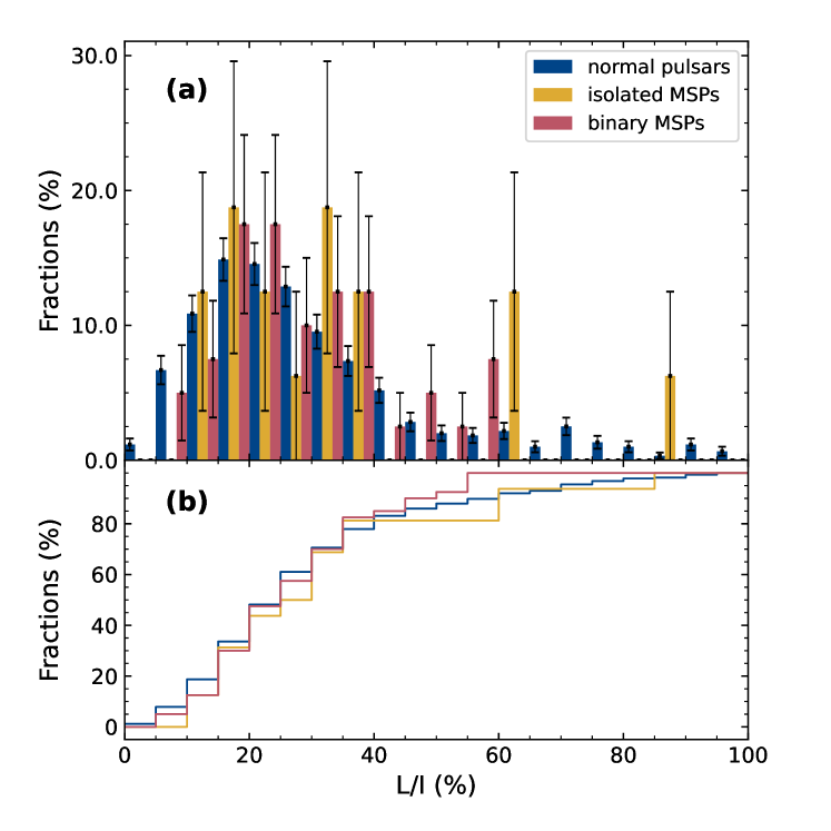
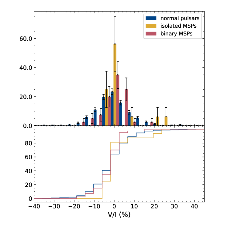
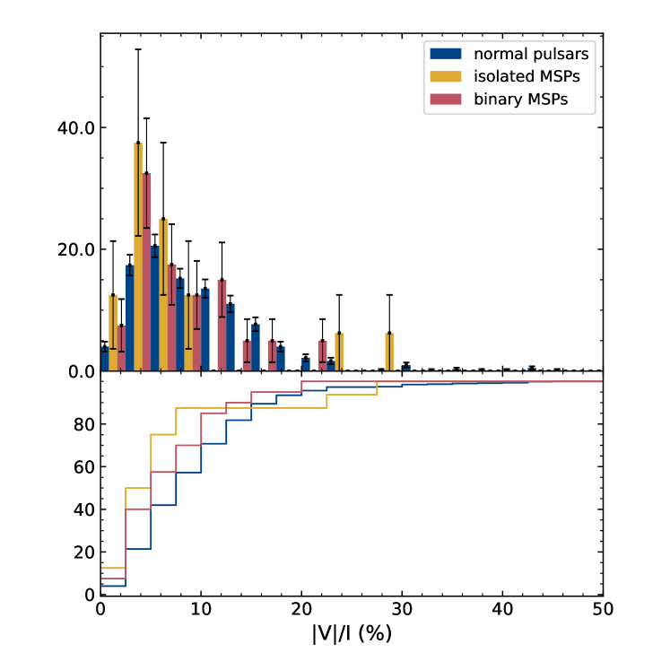
Figure 4: Distribution of polarization degree for 56 CPTA pulsars. The panels from left to right show the distribution for linear polarization, circular polarization, and the absolute value of circular polarization, respectively. The top row of panels shows the binned distribution function, while the bottom row is for the cumulative distribution function. Blue, yellow, and red colors denote the distribution for normal pulsars, isolated MSPs, and binary MSPs, respectively. Error bars are for the 68% confidence level computed from $1/\sqrt{N}$, with $N$ being the counts per each bin. The data for normal pulsars ($P_{0}>50\,{\rm ms}$) is from Wang et al. (2023).

The RM and DM of each pulsar are listed in Table 1. The averaged Galactic magnetic field strengths, in the directions of the pulsars, were estimated from $\left\langle B_{\|}\right\rangle=1.23\,\mu\mathrm{G}\left(\frac{\mathrm{RM}}{\mathrm{rad\cdot m^{-2}}}\right)\left(\frac{\mathrm{DM}}{\mathrm{pc\cdot cm^{-3}}}\right)^{-1}$. As is shown in Fig. 5 , the magnetic field distribution features reversal above and below the galactic plane, which is consistent with the previous study (Xu & Han 2014).

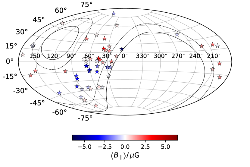
Figure 5: Averaged Galactic magnetic field parallel to the line of sight to CPTA pulsars in Galactic coordinates. Positive values indicate the Galactic magnetic field points toward the observers. The values shown here are derived from the ratios of RM and DM. The solid line denotes the sky coverage of FAST, while the dashed line presents the critical angle of $26.4^{\circ}$.

5 Discussion of the results

5.1 Weak emission of pulse profile

From the observed pulse profiles of CPTA pulsars, a significant fraction of MSPs show weak emission outside the traditional “on-pulse window,” which was defined as the pulse phases covering the pulse peak and a dominant fraction of pulse energy (Taylor & Huguenin 1971). Previously, Gentile et al. (2018) and Wahl et al. (2022) had detected 11 pulsars with “microcomponents;” that is, pulse components with peak intensities much lower than the total pulse peak intensity. Such microcomponents also appear in our data (e.g., in PSRs J1024$-$0719, J1713$+$0747, J2145$-$0750, and J2234$+$0944). We have discovered weak radiation in 44 pulsars. Furthermore, they present a very diverse phenomenology. In this way, it is hard for us to simply define the isolated components. We simply use the name “weak components” or “weak radiation” for a pulse structure with a flux lower than 3% of the peak flux.

It is well known that spectral leakage at the band edges and polyphase filter response functions introduce low-amplitude signal artifacts. In fact, any band-limited process will introduce artificial structures into the time domain. However, the weak components we found here do not belong to the instrumental artifacts mentioned above. We show the dedispersed dynamic spectra of eight pulsars in Fig. 6 . There is no apparent “reflection” at the band edges (i.e., frequencies close to 1500 MHz or 1000 MHz). Moreover, the weak components possess the same DM as the main pulse of the pulsars, since they also present as vertical strips after dedispersion.

The weak components are not narrowband features. As is shown in Fig. 6 , they span the entire bandwidth, from approximately 1000 MHz to 1500 MHz. In the time domain, these weak components are well separated from the high-flux pulse structures. For certain pulsars, such as PSR J0023$+$0923, there are distinct flux gaps between the weak components and the main pulse. The polarization properties of the weak components, as is demonstrated in Fig. 6 , differ significantly from those of main pulses in most pulsars. These three facts make it unlikely that the weak components arise from polyphase filter leakage.

However, we observe a new kind of artifact in CPTA pulsars that is different from previous studies. Examples of such artifacts are shown in Fig. 6 within the dynamic spectra of PSR J1713$+$0747. They present as weak inclined strips with different slopes. Such artifacts frequently appear in two bright pulsars, PSRs J1713$+$0747 and J2145$-$0750, but they also occur in weak pulsars such as PSR J0636$+$5128. Fortunately, these artifacts have a much lower amplitude than the weak components, and even noise level, so the integrated pulse profile is minimally affected. Further discussion on these artifacts can be found in Appendix C.

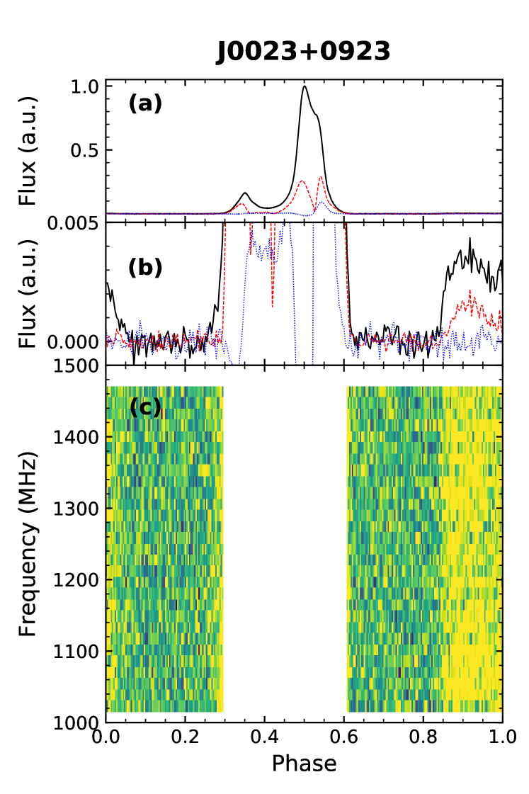
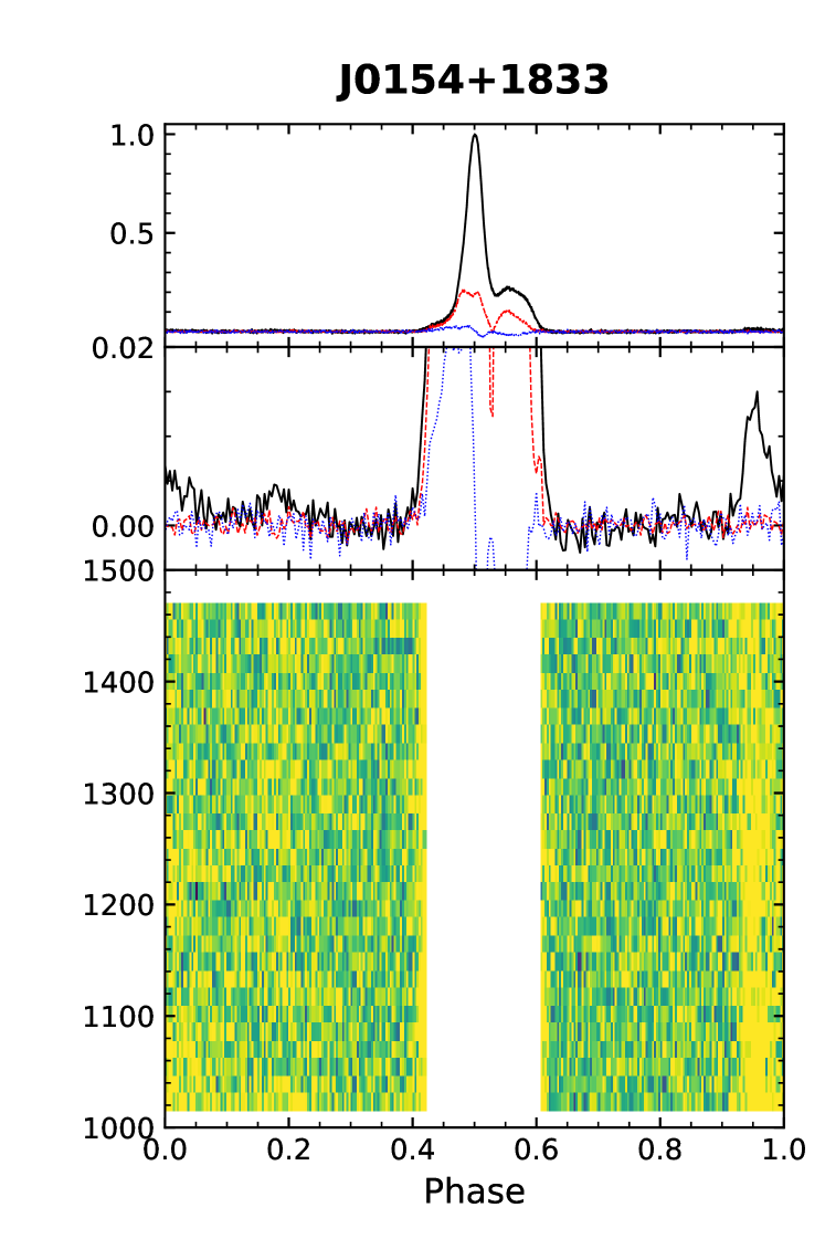
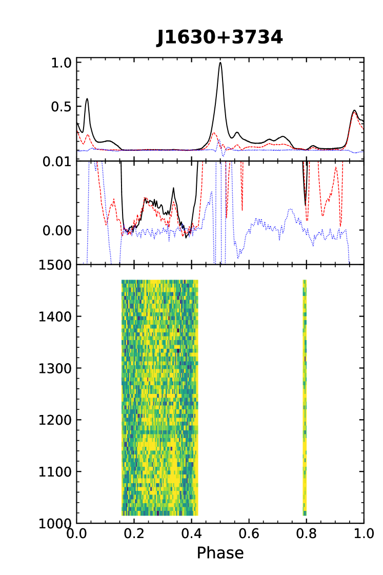
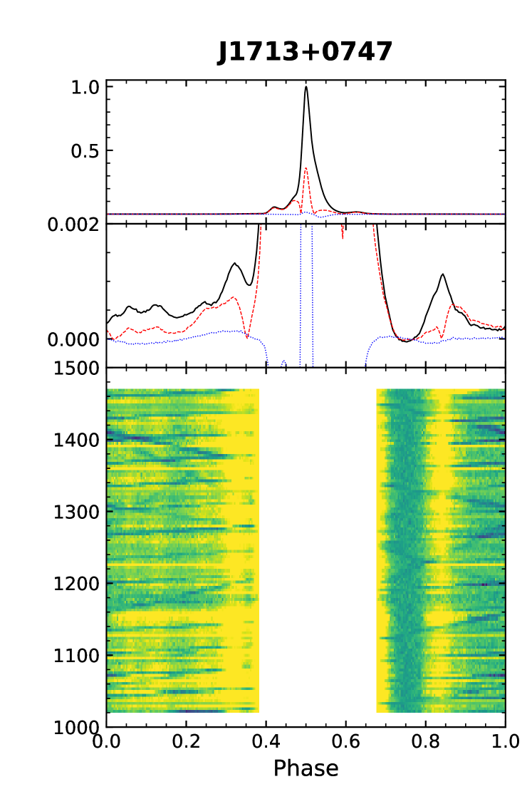
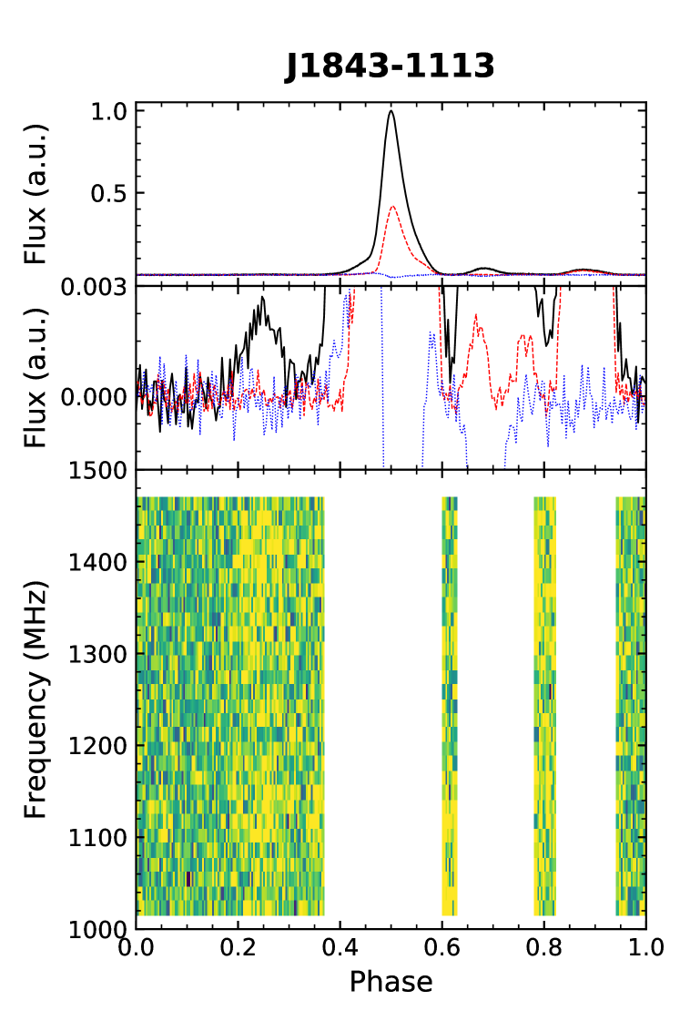
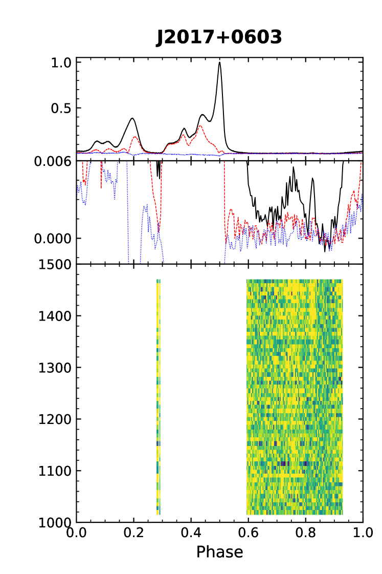
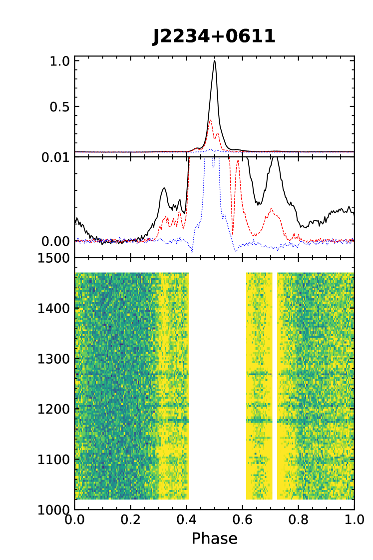
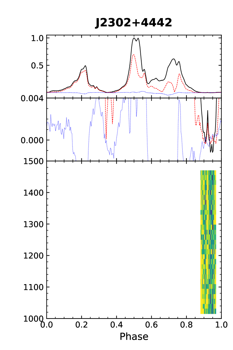
Figure 6: Dynamic spectra of weak components for eight CPTA MSPs. Panel (a) shows the full polarization profile, panel (b) zooms into the low-flux region to show the weak radiation or weak components, and panel (c) shows the dynamic spectra, where total fluxes larger than the range displayed in panel (b) are masked out (in white).

The weak radiation, besides forming extra pulse components, can also be a tail-like or prelude-like structure flanking the main pulse, such as in PSR J0340$+$4130, or bridge emission between pulse components, such as in PSR J1857$+$0943, or interpulse-like components, such as in PSR J0751$+$1807. In at least five pulsars (PSRs J0023$+$0923, J0154$+$1833, J0406$+$3039, J1946$+$3417, and J2234$+$0611), the weak emission components are spaced approximately 180^∘ from the main pulse, suggesting that those components are possibly from the other magnetic pole. These emerging components offer us new information about the radiation geometry, which will be discussed in a subsequent paper.

Most of the weak components show linear polarization, and we detect circular polarization in weak components for PSR J0406$+$3039, J0751$+$1807, J1713$+$0747, and J2145$-$0750. Some non-polarized weak components are also observed in PSR J0154$+$1833, J1843$-$1113, and J2234$+$0611. However, the current limited sample size prevents us from investigating whether the polarization properties of the weak components are significantly different from normal pulse components.

In terms of pulse width, the weak components last for about $10\%-20\%$ of full rotation. PSR J2017$+$0603, J2022$+$2534, and J2302$+$4442 show very narrow, spiky, weak components at the scale of less than 5% rotation. The timescales for the narrow weak components are around 50 $\mu s$. Such a small timescale indicates that the plasma beam powering such radiation has a rather limited angular diameter and implies an extremely nonuniform environment for the radiation regions.

5.2 Pulse width

As a common consensus, the pulse widths of MSPs are generally wider than the ones of normal pulsars. In the case of CPTA pulsars, as is listed in Table 1, the average value of the effective width is on the level of 10%, which is defined as the ratio of integrated flux divided by the peak flux (i.e., $W_{\rm eff}\equiv\int_{0}^{1}I(\phi)d\phi/I_{\rm max}$). The average and median for $W_{\rm eff}$ are 11% and 10%, respectively. The values are comparable to previous published results (Yan et al. 2011; Gentile et al. 2018). Such a pulse width exceeds that of normal pulsars, which is generally lower than $10\%$ (Gould & Lyne 1998; Johnston & Kerr 2018; Wang et al. 2023). The effective pulse width measurements indicate that the MSP radiation energy is still beamed, although it is more extended than that of a normal pulsar.

Instead of asking which phase range the most pulse energy is concentrated in, we can pose a different question: whether it is possible to detect pulsed radiation outside the pulse window. Our observations show that the detectable pulse width is much larger than the $W_{\rm eff}$. Here, the detectable pulse width ($W_{\rm det}$) is the total phase range where the flux is above three times the noise floor. We compare the effective pulse width ($W_{\rm eff}$) and the detectable pulse width ($W_{\rm det}$) in Table 1. The average and median of $W_{\rm det}$ for 56 MSPs are 65% and 70%, respectively. In this way, a small fraction of the radiation energy from an MSP spreads to a much larger solid angle, and nearly covers the full rotation phase.

The higher value of $W_{\rm det}$ is not caused by the interstellar scattering effect, with the exception of PSRs J1903$+$0327 and J1946$+$3417. Firstly, the pulse profiles show no obvious scattering tails for most pulsars in our list. Secondly, ISM models, such as the NE2001 and YMW models (Cordes & Lazio 2002; Yao et al. 2017), predict that the scattering timescale of CPTA pulsars is of only a few microseconds. This is naturally expected, as all the 56 MSPs here are observed for timing purposes. Their distance, DM, and scattering measure are all expected to be small compared to other MSPs.

If we extrapolate the radiation beam size – period relation derived for normal pulsars to MSPs (Gunn & Ostriker 1970; Lyne & Manchester 1988; Gil et al. 1993; Maciesiak et al. 2011), we would expect a correlation between $W_{\rm det}$ or $W_{\rm eff}$ and the pulsars’ spin periods and/or period derivatives. However, no significant correlations can be found, possibly because our sample size is very limited where the range of pulsar period is only approximately 1 dex. It is also possible that the different magnetosphere conditions for MSPs and normal pulsars erase such a correlation. For example, one argument is that the magnetospheres of MSPs are smaller than the ones of normal pulsars, so the multipolar magnetic field becomes important and radiation is less beamed (Krolik 1991; Kramer et al. 1998).

A large value for $W_{\rm det}$ may indicate that the MSPs radiate over the full rotation phase. As is mentioned in Sect. 4, six CPTA pulsars are promising candidates. If we lower the threshold of identifying the emission, in other words, identifying a signal above the 1-$\sigma$ noise level, another 13 pulsars are potentially 360^∘ radiators: PSRs J0030$+$0451, J0751$+$1807, J1024$-$0719, J1453$+$1902, J1630$+$3734, J1745$+$1017, J1832$-$0836, J1955$+$2908, J2017$+$0603, J2145$-$0750, J2214$+$3000, J2234$+$0944, and J2302$+$4442. For normal pulsars, a similar phenomenon had been reported before (Hankins & Cordes 1981; Rankin & Rathnasree 1997; Wang et al. 2022). Future monitoring of CPTA pulsars will further increase the integration time and S/N, which will help us to identify and confirm these 360^∘ candidates.

A large value of $W_{\rm det}$ and the weak radiation of MSPs may affect our predictions for future MSP searches using upcoming high-gain telescopes such as the Square Kilometre Array (SKA). In the near future, SKA will become operational, with pulsar searches being one of the key scientific objectives. As the telescope’s sensitivity increases, the combination of a large detectable pulse width and the weak radiation components observed in many MSPs will improve our chance of discovering more MSPs, because the weak radiation extends the size of the pulsar beam and increases the probability of detection.

5.3 Polarization properties

In this paper, we focus on investigating the frequency-integrated polarization pulse profiles of MSPs. The investigation of the frequency evolution of polarization properties will be published in the future. There are no significant differences between our polarization profiles and published results (Yan et al. 2011; Gentile et al. 2018; Spiewak et al. 2022), except for PSR J0154$+$1833. For this source, we had detected the presence of both linear and circular polarization, which was absent in the profile obtained by MeerKAT (Spiewak et al. 2022).

The polarization profiles of MSPs are more complex than ones of normal pulsars. We find that they may all belong to the “complex type” of Rankin’s classification scheme (Rankin 1983), and the detection of weak components makes the pulse profiles even more complex. The interpulse-like components show up in 25% of the 56 pulsars, including PSR J0023$+$0923, J0030$+$0451, J0154$+$1833, J0406$+$3039, J1453$+$1902, J1630$+$3734, J1857$+$0943, J1946$+$3417, J2017$+$0603, J2043$+$1711, J2150$-$0326, J2214$+$3000, J2234$+$0611, and J2322$+$2057. The more frequent appearance of interpulses in CPTA pulsars may be due to the larger radiation beam sizes, which makes it easier to catch up with the interpulse emission.

Across the pulse phase, most pulsars exhibit a higher degree of linear polarization at the edges of pulse components, consistent with the findings of Dai et al. (2015). This suggests an anticorrelation between the degree of linear polarization and flux intensity. This is consistent with the wave propagation model (see Fig. 9 of Wang et al. (2010)), which suggests that the wings of the pulse, due to their higher emission altitude, are less affected by propagation effects, and therefore exhibit a higher degree of linear polarization. On the other hand, such limb enhancement of linear polarization may indicate that all MSP pulse profiles are affected by the propagation effects.

We note that the sign of circular polarization can reverse multiple times across the pulse phase. Similarly, the sense of the PA sweep can also reverse. For instance, PSR J0613$-$0200 exhibits oscillatory patterns in both PA and $V$ within the main pulse window. Previous studies (Radhakrishnan & Rankin 1990; You & Han 2006) have suggested a correlation between the sense of circular polarization and the PA sweep in conal-double pulsars. However, for MSPs, it is difficult to define a global sense of the PA sweep and circular polarization, as multiple reversals of both occur quite frequently. The correlation may break down in MSPs. For example, both PSR J1744$-$1134 and J1745$+$1017 have negative $V$, but opposite senses for the PA sweep. We suspect that the complex magnetic field configuration introduces an extra ingredient into the propagation model. However, the local sense of circular polarization (sign of $V$) of a given pulsar may still correlate with the slope of the PA sweep. For example, in PSR J0824$+$0028, the first two peaks have $V<0$ and the third peak shows $V>0$, while the PA sweep sign is reversed for the third peak. A similar feature is also seen in PSR J1453$+$1902 and J0154$+$1833.

The PA jumps are common in CPTA pulsars, which are believed to be induced by the orthogonal polarization modes. We note that PA jump can be away from exactly 90^∘, as is shown in PSR J1630$+$3734. Also, the PA jumps seem to fall into two categories, I) the PA jumps when the polarization intensity goes to zero (e.g., in PSR J0154$+$1833), and II) the PA jumps around a local circular polarization peak (e.g., in PSR J0023$+$0923). The two types of PA jump can occur in the same pulsar. For example, the first PA jump of J0340$+$4130 is type I, while the second PA jump is type II. It is worth mentioning that the two types of jump show very different paths on the generalized Poincarè sphere: the type I PA jump happens when the polarization vector shrinks back to the origin (e.g., see (McKinnon & Stinebring 1998)), while the type II PA jump happens when the polarization vector goes through the north or south poles (Dyks 2020). The PA curves of many CPTA pulsars evidently deviate from the RVM model. Only five pulsars – PSRs J0605$+$3757, J0636$+$5158, J1903$+$0327, J2214$+$3000, and J2234$+$0611 – are found to be well described by the RVM model.

In the low-flux regime, we note that, sometimes, linear polarization has a flux that appears to be barely larger than the total intensity, as happened in PSRs J0509$+$0856, J1453$+$1902, J1630$+$3734, J1710$+$4923, J1713$+$0747, J1745$+$1017, and J1955$+$2908. This excess is not caused by our baseline selection. We note that the excesses remain, even if we reduce the baseline phase range. In the cases of PSRs J1713$+$0747 and J1955$+$2908, high-S/N data from the Arecibo telescope (Gentile et al. 2018) seem to show similar excesses at the same pulse phases; that is, phase 0.9 and phase 0.3 for PSR J1713$+$0747 and J1955$+$2908, respectively. Thus, the problem is more likely caused by small DC offsets in the polarization profiles. For example, if one adds a tiny DC offset to the total intensity pulse profiles, there will be no linear polarization excess. This indicates that those pulsars may also be 360^∘ radiator candidates. Indeed, the pulsar list here overlaps with the pulsar list showing a detectable width ($W_{\rm det}$) larger than 0.9 rotation. The interferometric observations can be used to determine the true baseline of the pulsar signal (Navarro et al. 1995; Marcote et al. 2019). We expect that future high-sensitivity arrays such as SKA will be able to provide better baseline estimation.

5.4 Apparent RM variation across the pulse phase

As is discussed in Sect. 3.2, the RMs of most pulsars are constant across the pulse phase. However, we detected residual “RM variations” across the pulse phase within some pulsars, as is shown in Fig. 3 for some examples. Such behavior should not be regarded as the intrinsic RM variation due to the Faraday rotation in the pulsar magnetosphere, as the relativistic plasma contribute only negligible RM (Wang et al. 2011). The apparent RM variation may be a consequence of pulse profile evolution in the frequency domain. We postpone this analysis to a future work focusing on the frequency evolution. As one can see, the apparent RM variation is more prominent at the phases where the PA jumps. In this case, the two orthogonal polarization modes with different spectral indexes will induce frequency-dependent variations in the PA (Ramachandran et al. 2004; Noutsos et al. 2009; Ilie et al. 2018). For PSRs J1903$+$0327 and J1946$+$3417, the RM variation may be a result of the interstellar scattering effect, which flattens the PA curves (Karastergiou 2009; Noutsos et al. 2009; Noutsos, A. et al. 2015).

5.5 Description of each pulsar

PSR J0023$+$0923: We detected a solitary weak component whose intensity is only $\sim 0.3$% of its highest peak. This component exhibits a higher degree of linear polarization than the main peak and has a flat PA. It is roughly separated from its main pulse region for 0.5 rotations. The PA jumps at phase 0.52 coincides with the reversal of circular polarization, while another jumps at phase 0.37 corresponds to the local peak.

PSR J0030$+$0451: The pulse width is approximately a full rotation phase. If we consider the weak components at the trailing edge of the interpulse (phase 0.15), the PA has a global linear trend across the full phase, although it shows complex structure around the main peak. The main pulse presents a higher polarization degree at its edges.

PSR J0034$-$0534: The pulse profile shows a dominant double-peak structure with a trailing pulse component, whose fractional linear polarization is much higher than the main pulse. There is a weak bridge emission at phase 0.7 at the level of 2% peak flux. The pulse signal covers more than 50% rotation. Similar to PSR J0030$+$0451, the PA shows a linear trend, outside the main peak.

PSR J0154$+$1833: The profile contains two weak components that form the interpulse (phase 0.2 and 0.95). They are separated from the main pulse by approximately half a rotation, which is similar to the case of PSR J0023$+$0923. No polarization is detected for them. There is a 90^∘ PA jump around the main pulse peak (phase 0.53), where both linear polarization and circular polarization decrease to zero.

PSR J0340$+$4130: We detected two weak components with peaks at the leading edge and the trailing edge (phase 0.1 and 0.8), respectively. Both of these components exhibit moderate degrees of polarization. The PA curve exhibits four 90^∘ jumps in the pulse window (phase 0.4-0.6), while the circular polarization shows no corresponding variation at these phases. The PA curve presents smooth variation outside the pulse window.

PSR J0406$+$3039: The pulse profile shows a weak component roughly 50% rotation away from the main pulse (phase 0.05). It shows a 90^∘ PA jump in the main pulse (phase 0.54) where the circular polarization reaches a local maximum. Similarly, the PA curve presents a monotonic decreasing trend across the whole pulse phase.

PSR J0509$+$0856: The pulsar shows radiation for nearly the full rotation. The PA curve is rather flat, except at the leading edge of the peak with a lower flux. The 90^∘ PA jump occurs at phase 0.04 and 0.9.

PSR J0605$+$3757: There is a weak bridge emission between the main pulse and the trailing weak pulse (phase 0.7). Unlike the main pulse, the weak trailing component presents extremely low linear polarization. The PA curve seems to follow the S-shape curve in the pulse window, although there are 90^∘ PA jumps at the center of the pulse peak (phase 0.5). The derived magnetic inclination angle, $\alpha$, is $0.9^{\circ}\pm 9.7^{\circ}$, and the sight angle, $\zeta$, between the line of sight and the spin axis is $0.7^{\circ}\pm 7.6^{\circ}$.

PSR J0613$-$0200: There are weak pulse components at the leading and trailing edges (phase 0.2 and 0.8). We are inclined to treat them as separated components, as PA variations in the weak components are smoother than the one in the main pulse. The PA jumps occur frequently across the pulse phase, and some of them coincide with the sense reversal or the local extremum of circular polarization. At phase 0.67, both linear and circular polarization decrease to zero.

PSR J0621$+$1001: The pulse profile has a double-peaked shape, and the two peaks are connected by bridge emission (phase 0.3). There is a weak component at the leading edges of the peak with a lower flux (phase 0.1). There is a roughly 90^∘ PA jump between the leading weak component and the main pulse (phase 0.1). In addition, PA jumps are frequent within the main pulse, one of which occurs at the local maximum of circular polarization around phase 0.48.

PSR J0636$+$5128: There is a weak component at the leading edges of the pulse (phase 0.3). A nearly 90^∘ PA jump occurs near the center of the pulse peak (phase 0.46). From the PA curve, we can derive the radiation geometry of $\alpha=6.5^{\circ}\pm 28.5^{\circ}$ and $\zeta=11.9^{\circ}\pm 49.0^{\circ}$. We should caution that the pulse width of this pulsar is narrow, which causes large uncertainty in the fitting result.

PSR J0645$+$5158: It has a bridge-like weak component between the main pulse and interpulse (phase 0.7). Although this weak component is connected to the interpulse, it may not be the weak leading edge of the interpulse, due to its long duration and low degree of polarization compared to that of the interpulse. A 90^∘ PA jump occurs near the center of the pulse peak (phase 0.5) where the circular polarization changes its sign. Compared with the main pulse, the interpulse shows a smoother PA curve.

PSR J0732$+$2314: This pulsar has an S-shaped PA swing in the main pulse window. However, the PA becomes very complex for the leading pulse (phase 0.1). There are bridge-like emissions (phase 0.2) between the two pulse peaks separated by approximately 180^∘. Two PA jumps occur at phase 0.1 and 0.42, which coincides with the sense reversal of $V$.

PSR J0751$+$1807: We detect a weak component preceding the leading edge of the main pulse (phase 0.1), and a wide weak component at phase 0.8 spanning for $\sim 0.3$ rotations. Both of them exhibit a low degree of polarization. PA jumps occur multiple times over the whole phase, two of which, at phase 0.12 and 0.42, are orthogonal. The circular polarization reaches the local extremum at jump phase 0.42 and changes sign at jump phase 0.52.

PSR J0824$+$0028: There seem to be no weak components for this pulsar. Unlike the main pulse, the interpulse at phase 0.1 is nearly 100% linearly polarized. The former two pulse components present a different sense of circular polarization than the main pulse.

PSR J1012+5307: There are three peaks on the pulsar’s pulse profile. The weaker peaks from phase 0.8 to 1 may be an interpulse. However, we detected bridge emission at a level of 1% of the peak flux connecting to the main pulse (phase 0.7). A PA jump occurs at the leading edge of the interpulse around phase 0.75. The PA curve of the main pulse has a good S-shape.

PSR J1024$-$0719: We find that there is weak bridge emission between the leading weak component and the main pulse (phase 0.1-0.4). There is also a trailing weak component (phase 0.9) with an intensity of $\sim 0.5\%$ of the highest peak and nearly 100% degree of linear polarization at the spin phase of $\sim 0.9$. 90^∘ PA jumps occur at the leading and trailing edges of the main pulse (phase 0.12, 0.35, and 0.64).

PSR J1327$+$3423: No weak component is detected. A 90^∘ PA jumps occurs at the leading edges of the pulse (phase 0.45) and the jump at phase 0.52 is non-orthogonal.

PSR J1453$+$1902: This is a rather weak pulsar, even for FAST. The pulse component at phase 0.2 has a much higher linear polarization degree than the main pulse. A weak component is present at the phase of $\sim 0.82$ in the profile. In addition, we identity a rather weak interpulse with an intensity of 2% of the main pulse (phase 1.0). There are possible 90^∘ PA jumps at the trailing edge of the main pulse (phase 0.67). We note that there is a non-orthogonal PA jump accompanied by a small spike in the degree of circular polarization around the main peak (phase 0.53).

PSR J1630$+$3734: A very weak component with a nearly 100% degree of linear polarization is located between the interpulse and the main pulse (phase $\sim 0.3$). The intensity of this component is only about 0.4% of that of the highest peak. The PA curve presents multiple jumps, which are nearly 90^∘ except for those around the main pulse. Some of them are accompanied by a sign change in circular polarization at phase 0.1, 0.50, 0.52, and 0.8.

PSR J1640$+$2224: Four PA jumps happen within this pulsar, one of which coincides with the sense reversal of $V$ at phase 0.53.

PSR J1643$-$1224: The pulse width seems to be rather wide, with the leading edge extending for more than half the rotation. Both orthogonal and non-orthogonal PA jumps are visible, some of which occur at the phase of the sense reversal of $V$ (phase 0.36, 0.49, and 0.53).

PSR J1710$+$4923: This pulsar radiates over the full rotation phase, and a weak component is observed around phase 0.1, which contains a low polarization degree. The PA jumps are common in this pulsar, three of which are nearly $90^{\circ}$, at phase 0.21, 0.28, and 0.34, respectively. The circular polarization profile reaches the local maximum at jump phase 0.45 and 0.64.

PSR J1713$+$0747: This is a well-known pulsar; however, our data show that the pulsar radiates over nearly the whole period. We note that this pulsar has an interpulse-like structure at phase 0.85. The leading component spans roughly 40% of the rotation phase. There are several PA jumps for this pulsar, either in the main pulse peak or in the weak components. Except for the one at phase 0.59, they are all orthogonal. Two jumps around the flux peak are accompanied by a sign change in the circular polarization profile. After correcting the PA jumps, the PA curve has an S-shape. The RVM model gives the geometry of $\alpha=48.0^{\circ}\pm 5.6^{\circ}$ and $\zeta=74.7^{\circ}\pm 6.8^{\circ}$.

PSR J1738$+$0333: No weak component is detected. The PA curve swings rapidly at the trailing edge of the main pulse.

PSR J1741$+$1351: No weak component is detected. Several PA jumps happen within the main pulse. At phase 0.52, both linear and circular polarization reduce to zero.

PSR J1744$-$1134: A weak component is observed at phase 0.15. The main pulse is nearly 100% linearly polarized, while the weak components have a lower linear polarization degree. In addition, the PA curve of the main pulse is smoother. The 90^∘ PA jumps occur around the pulse peak (phase 0.45 and 0.6).

PSR J1745$+$1017: The profile exhibits weak components at phase 0.05 and 0.9, both of which are highly linearly polarized. This pulsar is also a potential $360^{\circ}$ radiator, since the linear polarization flux is higher than the intensity flux at phase 0.35.

PSR J1832$-$0836: This pulsar has a very complex pulse profile that spans nearly the whole pulse phase. A weak component with a high degree of linear polarization is situated between the two highest peaks. Additionally, a bump-like weak component precedes the low-intensity peak (at phase 0.05 in this study). PA jumps are common in this pulsar. At jump phase 0.77, the linear polarization decreases to zero, while the circular polarization shows as a peak.

PSR J1843$-$1113: The profile shows a weak component preceding the main pulse (phase 0.25), with an intensity that is only 0.2% of the highest peak. There is no detectable polarized emission in this weak component. Additionally, we have detected weak bridge emission between the three prominent peaks. No PA jump is detected.

PSR J1853$+$1303: The profile shows a weak bridge emission (phase 0.7) connecting the main pulse and the interpulse. PA jumps occur frequently in this pulsar. There are four jumps accompanied by sign changes in $V$ at phase 0.44, 0.51, 0.56, and 0.58, respectively.

PSR J1857$+$0943: The profile shows a weak bridge emission (phase 0.3) connecting the main pulse and the interpulse. The PA curve has a complex shape, and presents a rapid sweep between phase 0.4 and 0.6.

PSR J1903$+$0327: The profile shows a scattering-like pulse tail. Neither a PA jump nor a weak component is detected. The RVM model gives the radiation geometry of $\alpha=0.4^{\circ}\pm 3.6^{\circ}$ and $\zeta=0.8^{\circ}\pm 8.2^{\circ}$. However, we should caution that such a result may be influenced by the scattering effect.

PSR J1910$+$1256: No weak component is detected. Nearly $90^{\circ}$ PA jumps occur around the peak, one of which corresponds to the sense reversal of $V$ (phase 0.5).

PSR J1911$-$1114: No weak component is detected. A $90^{\circ}$ PA jump is observed at phase 0.6. The leading component at phase 0.35 has a much higher linear polarization degree and a smoother PA curve.

PSR J1911$+$1347: There is weak radiation at the trailing edge of the main pulse (phase 0.8-0.9). Weak bridge emission is also detected around phase 0.6. The PA jump at phase 0.51 coincides with the sign change of $V$.

PSR J1918$-$0642: The pulse profile has two peaks separated for a roughly 0.5 rotation. No clear weak pulse component is detected. There is also no bridge emission between the main pulse and the interpulse down to the level of a few thousandths of the peak flux. This indicates that the interpulse comes from the other magnetic pole. The PA curve has a complex shape in which PA jumps are frequent within the main pulse. One of them occurs at phase 0.56 which is of little offset to the local peak of $V$. Two jumps at phase 0.44 and 0.48 coincide with the sense reversal of V.

PSR J1923$+$2515: A weak component at phase 0.95 is detected that is connected to the interpulse at phase 0.15. A bridge emission of 1% peak flux around phase 0.4 is also observed between the main pulse and the prevailing component. We notice that they have different fractional polarizations. Two PA jumps at phases 0.49 and 0.61 are a little offset from the local peak of $V$.

PSR J1944$+$0907: This pulsar is a candidate radiating over the full rotation. We observe a weak component at the leading edge of the main pulse (phase 0.3). The PA curve apparently deviates from the S-shape. The profile V reaches local maximum at jump phase 0.6.

PSR J1946$+$3417: There is a weak component separating from the brightest peak for half a rotation (phase 0), and it shows roughly a 70% degree of linear polarization. We observe two weak bridge emission regions (phase 0.3 and 0.7). Similar to J1903$+$0327, the interstellar scattering effect is also obvious. PA jumps happen around the main pulse peak (phase 0.5) and around the bridge emission region (phase 0.34, 0.78, and 0.83).

PSR J1955$+$2908: There is weak bridge emission (phase 0.3) between the weak interpulse and main pulse. As one can see, the linear polarization is apparently higher than the total intensity. One possible explanation is that the baselines of the polarization profiles have not been subtracted correctly, indicating that it could be a full-phase pulsar. PA jumps happen in the main pulse phase (phase 0.44 and 0.52). The PA curve presents a rapid swing after phase 0.52.

PSR J2010$-$1323: A weak component with a long leading tail is observed at phase 0.4. It exhibits a higher degree of linear polarization than the main pulse. The circular polarization changes its sign at jump phase 0.49 and reduces to zero with linear polarization at phase 0.56.

PSR J2017$+$0603: Two distinct weak components are detected, following the trailing edge of the brightest pulse (phase 0.7-0.8). Both of them show a moderate degree of linear polarization. Their fluxes are only 0.4% of the peak flux. We also notice a very weak bridge emission between the main pulse and the interpulse at phase 0.3. Four PA jumps happen at phase 0.09, 0.18, 0.3, and 0.5. At phase 0.18, the circular polarization changes its sign. It reaches the local maximum when linear polarization reduces to zero at phase 0.5. Although the PA curve is smooth, the RVM model cannot give a reasonable result, which may be due to the non-orthogonal jump at phase 0.3.

PSR J2019$+$2425: A weak bridge emission at a level of 2% of the peak intensity between the main pulse and the leading component is detected (phase 0.3). The PA curve shows a sudden dip at the phase around 0.43, which may be due to an OPM transition. We notice that the directions of the sense reversal of circular polarization are opposite for the main pulse and the trailing component. A $90^{\circ}$ PA jump is detected in the trailing components (phase 0.82), where the V changes its sign.

PSR J2022$+$2534: There may be a weak component at phase 0.9. PA jumps occur around the main pulse peak, which are both accompanied by a sense reversal in V. In addition, the leading pulse component presents much steeper PA slopes than the main pulse. Sense reversal of circular polarization happens multiple times in this pulsar.

PSR J2033$+$1734: The extended trailing component covers roughly 30% of the spin period. Unlike the main pulse, it presents violent PA variations. There may be a weak component around phase 0.85. Sense reversal of circular polarization occurs several times. Both a PA jump and sense reversal emerge at the main pulse peak (phase 0.5).

PSR J2043$+$1711: A weak component of 2% $I_{\rm max}$ at phase 0.1 and low-level bridge emission around phase 0.8 are detected. The PA jumps are observed at its trailing component (phase 0.7).

PSR J2145$-$0750: A weak component of 0.4% $I_{\rm max}$ at phase 0.9 and the bridge emission of 0.2% $I_{\rm max}$ at phase 0.4 are observed. The new detected weak component and the interpulse (at phase 0.3) contain different fractional linear polarizations from the main pulse. The main pulse and interpulse have different senses of circular polarization. The PA curve is complex and the PA jumps are common.

PSR J2150$-$0326: No weak components are detected in this pulsar. The PA jump happens within the interpulse at phase 0.1, where V changes sign. The sense reversals of circular polarization occur at phases near the main pulse peak. At phase 0.5, before the main pulse peak, we note that a circular polarization peak coincides with a local PA sweep.

PSR J2214$+$3000: Two weak components are observed, one at the leading edge of the main pulse (phase 0.3) and another one between the main pulse and the interpulse (phase 0.7-0.8). We also found two bridge emission regions, one connecting the main pulse and the second weak components (phase 0.3) and another one between the second weak component and interpulse (phase 0.7). The intensities of both weak bridge emission are at the level of 0.2% of the peak flux. All those weak components appear to be highly linearly polarized. There is a PA jump around phase 0.35, shortly before the main pulse peak. The PA curve has an S-shape, although it presents little deviation at phase 0.05. From the RVM model, we derive $\alpha=31.6^{\circ}\pm 3.7^{\circ}$ and $\zeta=30.3^{\circ}\pm 4.5^{\circ}$. This contrasts with the presence of the interpulse, which supposed to be from another magnetic pole. Similar cases are also discussed in PSR B0950$+$08 (Hankins & Cordes 1981) and PSR B1929$+$10 (Rankin & Rathnasree 1997). We leave this to future work.

PSR J2229$+$2643: No weak components are observed. The sense reversals of circular polarization occur around phases 0.4 and 0.55.

PSR J2234$+$0611: We found three weak components, two of which flank the main pulse (phase 0.3 and 0.7). The third one at phase 0 is very weak and wide (it extends to the second weak component at the trailing edge of the main pulse). The third weak component separates from the main peak for about 0.5 rotation, indicating that it is possibly the interpulse of this pulsar. A PA jump is seen at the trailing edge of the main peak (phase 0.57), accompanied by the sense reversal of V. Similar to J2214$+$3000, the fitting result on the PA curve gives $\alpha=8.1^{\circ}\pm 7.1^{\circ}$ and $\zeta=14.7^{\circ}\pm 12.7^{\circ}$, which suggests a nearly aligned rotator.

PSR J2234$+$0944: The pulsar is potentially radiating for the full rotation. We found a weak component at phase 0.2, whose intensity is only 0.2% of that of the highest peak. There is bridge emission of less than 1% between the two pulse peaks (phase 0.7). Both orthogonal and non-orthogonal PA jumps occur in this pulsar. In addition, the PA curve of the main pulse precursor seems to follow an S-shaped swing.

PSR J2302$+$4442: We identify a weak, distinct, and narrow component around phase 0.9 and weak bridge emission between the main pulse and the interpulse around phase 0.35. These components make this pulsar a potential $360^{\circ}$ radiator. A $90^{\circ}$ PA jump occurs at phase 0.34, where V changes its sign. Although the PA curve cannot be described by the RVM model, the curves of the main pulse and the interpulse have separate S-shapes.

PSR J2317$+$1439: We found a weak component with a plateau at the trailing edge of the main pulse (phase 0.9-1.0). The flux of this weak component is roughly 0.1% of that of the highest peak. The PA curve has a complex shape. The degree of circular polarization peaks around the second pulse peak and coincides with a dip in the PA curve. Both linear and circular polarization reach the local minimum at jump phase 0.53. Circular polarization arrives at local maximum at phase 0.65.

PSR J2322$+$2057: No weak component is detected. The pulse profile shows two peaks with approximately 0.4 rotation separation. At phase 0.04 and 0.6, the PA curve presents jumps coinciding with the sense reversal of V.

6 Conclusions

As a summary, the major conclusions in this paper are: 1) The polarization profiles for 56 CPTA pulsars are presented. Most of them are compatible with previous publications, but have higher S/Ns to shed light on the detail of structures. The polarization profiles of three pulsars – PSR J0406$+$3039, J1327$+$3423, and J2022$+$2534 – are published for the first time. 2) We find that there is no difference between the distribution functions of the polarization percentage between MSPs and normal pulsars. 3) Radiation below 3% of the pulsar peak flux are detected for 80% of pulsars, which implies that the microcomponents may be a common feature among MSPs. In addition, some pulsars may sustain radiation over the whole rotation period. 4) PA jumps are detected in the majority of MSPs. Two types of PA jumps can coexist in the pulse profile, in which the type I PA jump happens when the polarization flux drops to 0 and the type II PA jump is accompanied by nonzero circular polarization. 5) Polarization properties imply that the wave propagation effects in the MSP magnetosphere are important for the shape of the polarization pulse profile.

Data availability

The data of polarization pulse profiles are available at https://psr.pku.edu.cn/publications/CPTADR1/, and the corresponding figures are published at https://doi.org/10.5281/zenodo.14801349.

Appendix A Comparison of polarization profiles at small and large zenith angles

Although the backward illumination strategy facilitates FAST to observe sources with zenith angles larger than 26.4^∘, the main beam axis is not aligned with principal axis of the illumination area in this case. The misalignment causes angular separations between the left and right circular beams, known as beam squint and elliptical illumination patterns called as beam squash (Chu & Turrin 1973; Heiles et al. 2001a; Heiles 2002; Robishaw & Heiles 2021). Consequently, the polarization profiles derived at large zenith angles (¿26.4^∘) may be different from those obtained at small zenith angles ($\leqslant$26.4^∘).

Nearly half of the CPTA pulsars have both observations taken at small and large zenith angles. For each pulsar, after combining all observations at both kinds of zenith angles separately, a rough estimation on the effect of backward illumination can be made by comparing the derived integrated polarization profiles. Because of the three reasons, 1) such effect may be frequency dependent, 2) pulse profile evolves along the frequency, and 3) ISM effects, such as scintillation and scattering, are frequency dependent, we need to compare polarization profiles per frequency channel. The observation band is thus divided into several sub-bands. For each channel, we compute the difference in polarization profiles between the large and small zenith angle observation.

To obtain reliable result, we align, rescale and rebaseline the two pulse profiles and then subtract them to get the difference. The profiles alignment is performed in the Fourier domain (Taylor 1992). Then, since the two profiles have different S/N and baselines, they need to be matched before the subtraction as explained by Men et al. (2019); Jiang et al. (2022). The profile matching is obtained through minimizing $\chi^{2}$ defined as,

$$\chi^{2}_{\nu}=\left(\mathbfcal{P}_{\nu}-\alpha_{\nu}\mathbfcal{T}_{\nu}-\beta_{\nu}\right)^{2},$$ (10)

where $\mathbfcal{T}_{\nu}$ and $\mathbfcal{P}_{\nu}$ are polarization profile vectors normalised by respective noise levels at central frequency $\nu$. The integrated profiles at small zenith angle is taken as template $\mathbfcal{T}_{\nu}$. The scalar parameters $\alpha_{\nu}$ and $\beta_{\nu}$ are S/N scaled and profile baseline offset for the large zenith observations. The minimization of $\chi^{2}$ leads to

$$\alpha_{\nu}=\frac{\mathbfcal{P}_{\nu}\cdot\mathbfcal{T}_{\nu}-\frac{1}{N}\sum_{i}\mathcal{P}_{\nu,i}\sum_{i}\mathcal{T}_{\nu,i}}{\sum_{i}\mathcal{T}_{\nu,i}^{2}-\frac{1}{N}\sum_{i}\mathcal{T}_{\nu,i}\sum_{i}\mathcal{T}_{\nu,i}},$$ (11)

$$\beta_{\nu}=\frac{1}{N}\sum_{i}(\mathcal{P}_{\nu,i}-\alpha\mathcal{T}_{\nu,i}),$$

where $N$ is the number of bins of the profiles. The residual profiles are then accumulated across the frequency to obtain the final profile differences that

$$\delta\mathbfcal{P}=\int\left(\mathbfcal{P}_{\nu}-\alpha_{\nu}\mathbfcal{T}_{\nu}-\beta_{\nu}\right)d\nu\,.$$ (12)

Furthermore, to compare the difference in a reliable fashion, the integrated polarization profiles should be of high S/N for both small zenith and large zenith angles, which requires a long observation time. Only for PSRs J0636$+$5128 and J2033$+$1734, we have enough observations for both conditions. As shown in Fig. 7 , the maximal differences in polarization profiles between large and small zenith angle is at the level of 0.2%, barely above noise floor to be visible. These findings are consistent with previous studies(Jiang et al. 2020, 2022).

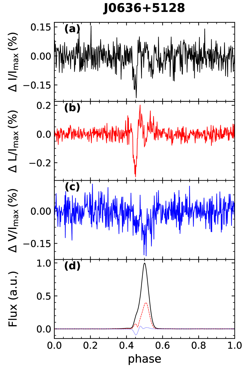
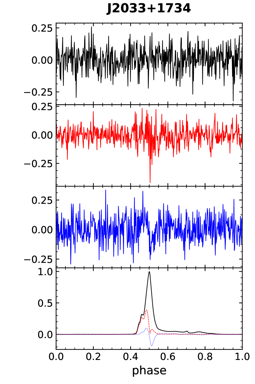
Figure 7: Polarization profile differences between small and large zenith angle observations for PSRs J0636$+$5128 and J2033$+$1734, which contain enough number of observations. Panel (a), (b), (c) are the profile residuals for total intensity, linear and circular polarization, respectively. Panel (d) is the polarization profile from small zenith angle observations. The black, red, and blue represents total intensity, linear, and circular polarization, respectively. We normalize all the curves, such that the peak total intensity is 1.

Appendix B Comparison of RM derived with the Bayesian and RM synthesis

We had computed the RM value from two methods, the Bayesian $Q$-$U$ fitting and the generalized RM synthesis. The averaged absolute differences of all observations between these two methods are given in Fig. 8 . As one can see, the difference between the two method is close to zero for most of the CPTA pulsars, and the difference is within statistical fluctuation.

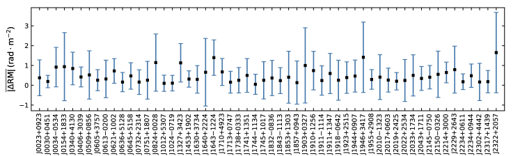
Figure 8: Averaged absolute differences between RM values derived with the Bayesian $Q$-$U$ fitting and the generalized RM synthesis. The error bars indicate the 68% confidence level (1-$\sigma$).

Appendix C Weak artifacts in dynamic spectra

We have detected weak artifacts in pulsar dynamic spectra shown in Fig. 9 . These dark inclined strip-like artifacts are detected mostly in bright pulsars, i.e. PSR J1713$+$0747, J1744$-$1134 and J2145$-$0750. For the three pulsars, the occurrence rates are $80\%$, $28\%$, and $31\%$ respectively. We note that the amplitudes of these artifacts correlate to signal strengths of pulsar signals, as they are only found in observations with high SNRs. Additionally, PSRs J1713$+$0747 and J2145$-$0750, which exhibit these artifacts most often, are the strongest pulsars in CPTA sample. In addition to the three pulsars mentioned above, we also detected such weak artifacts for a few occurrences ($<20\%$) in PSR J0030$+$0451, J0621$+$1002, J0636$+$5128, J0645$+$5158, J1327$+$3423, J1640$+$2224, J1857$+$0943 and J2229$+$2643.

Similar weak artifacts were also observed in other works (Yuan et al. 2023), where it was claimed to be weak interference. We believe that the artifacts are not the radio frequency interferences (RFIs) themselves. RFIs are concentrated in narrow bands and are much brighter than pulsar signal, while the weak artifacts exhibit a lower flux density than the noise floor and occupy the full bandwidth. They look similar to a previous case (Alam et al. 2020), where one can see artifacts as the mirror of dispersed signal about the central frequency. In contrast to the artifact reported by Alam et al. (2020), the artifacts we found are significantly weaker, which is below the noise floor. In addition, Alam et al. (2020) concludes that the artifacts were induced by mismatch between the interleaved analog-to-digital converters (ADC; Kurosawa et al. 2001). It is unlikely that ADC alone causes artifacts we detected. The FAST digital backends adopt the KatADC board, which is mounted with the ADC chip ADC08D1520 (from Texas Instruments https://casper.berkeley.edu/wiki/KatADC). The two ADC cores are not used in the interleaved mode, so we do not expect the artifact is due to the same reason as in the case of Alam et al. (2020).

The artifact is probably not caused by the leakage of polyphase filter banks alone, which, instead of creating a ‘dip’, introduces low amplitude power excess. We note that the artifacts follows a band-flipped DM signature as shown in Fig. 9. The dip appears at the lowest frequency at the time pulsar signal enters the highest frequency channel. As the dispersed pulsar signal drifts towards lower frequency, the dip turns to higher frequency. Other artifacts are tracks of dips being parallel shifted of the dispersed signal in frequency for $1/4$ and $1/2$ of the full band. As the FAST backend design used a four-tap polyphaser filter bank, it is likely that the artifact is caused by a combination of polyphaser filter leakage and digitizing of strong signal.

We could not track down the exact reason for the artifacts, which is left for future detailed studies. Instead, we evaluate the impact of the artifacts on the data quality. We combine observations with and without weak artifacts separately to form and compare integrated polarization profiles as shown in Fig. 10 . Luckily, we found that the major difference is only a slight offset of linear polarization intensity at the level of 0.1%, well below any effects we are trying to address in the current work.

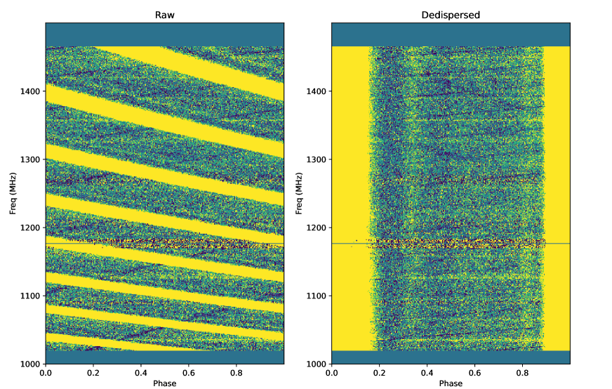
Figure 9: Dynamic spectrum of weak artifacts in observation for PSR J1713$+$0747, i.e. signal flux as function of frequency (y-axis) and pulse phase (x-axis). Left: raw dynamic spectrum without dedispersion. Right: dedispersed dynamic spectrum. The dynamic spectrum is intentionally saturated to enhance visual inspection of the weak artifacts.

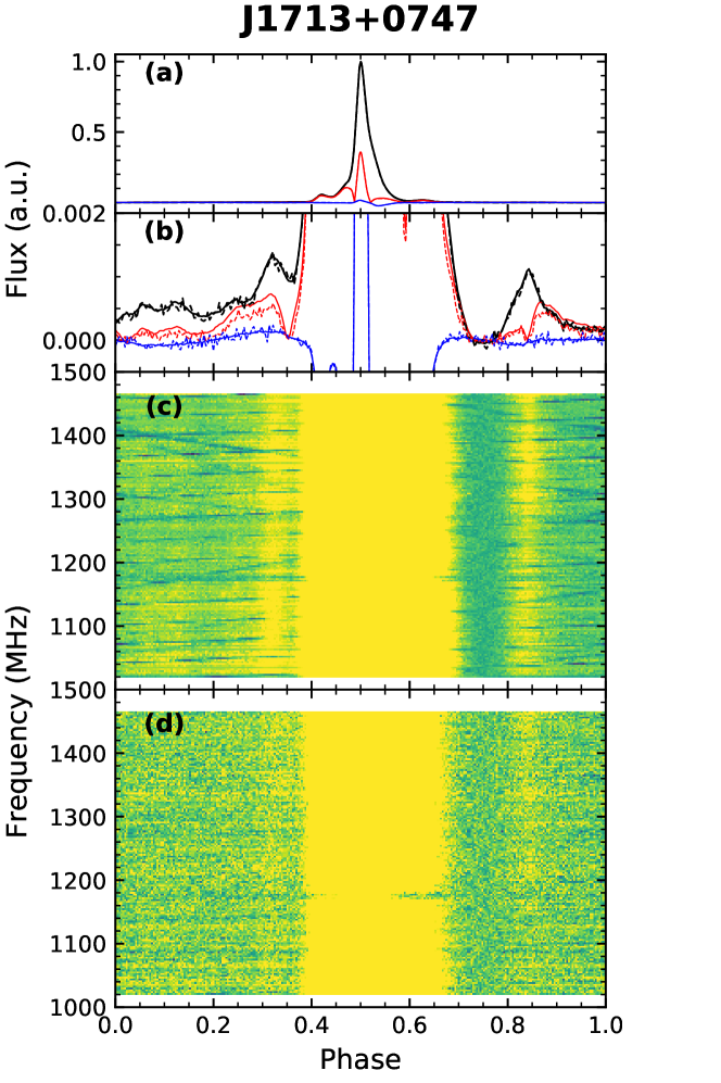
Figure 10: Comparison of profiles with and without weak artifacts. Panel a), polarization pulse profile of PSR J1713$+$0747 using the same color code as other plots in the paper. Panel b), pulse profiles from data with (solid curves) and without (dashed curves) artifact. Panel c) and d), dynamic spectra for data with and without artifact, respectively.

Appendix D Basic parameters for CPTA pulsars

Table 2: Parameters of 56 CPTA pulsars. All error bars are of 68% confidence level. Systematics $\rm\Delta DM_{\rm sys}$ and $\rm\Delta RM_{\rm sys}$ are estimated from the standard deviation for all observations, i.e. the values are for the DM/RM fluctuation or evolution over time.

Pulsar	Obs.dura.	Nobs	Length	DM	$\Delta{\rm DM_{sys}}$	RM	$\Delta{\rm RM_{sys}}$	B∥
	MJD		min	$\mathrm{pc\cdot cm^{-3}}$	$10^{-4}\mathrm{pc\cdot cm^{-3}}$	$\mathrm{rad\cdot m^{-2}}$	$\mathrm{rad\cdot m^{-2}}$	${\rm\mu G}$
J0023$+$0923	58907$-$59840	56	1281.5	14.33201 (16)	2.3	-5.6 (8)	0.6	-0.50 $\pm$ 0.07
J0030$+$0451	58883$-$59851	57	1290.0	4.33235 (4)	2.0	1.55 (23)	0.5	0.40 $\pm$ 0.13
J0034$-$0534	58956$-$59827	13	358.6	13.7764 (11)	6.0	9.2 (6)	1.4	0.78 $\pm$ 0.11
J0154$+$1833	58907$-$59697	23	450.0	19.79691 (10)	1.2	-19.6 (16)	2.1	-1.42 $\pm$ 0.07
J0340$+$4130	58684$-$59840	66	1693.0	49.58564 (24)	4.0	52.8 (5)	0.8	1.332 $\pm$ 0.016
J0406$+$3039	59403$-$59847	30	609.9	49.37599 (35)	2.5	64.00 (26)	0.4	1.588 $\pm$ 0.009
J0509$+$0856	58962$-$59848	35	681.9	38.32843 (18)	3.1	43.4 (11)	0.8	1.410 $\pm$ 0.024
J0605$+$3757	58962$-$59830	14	268.9	20.9433 (4)	5.0	4.34 (24)	0.4	0.247 $\pm$ 0.019
J0613$-$0200	58686$-$59849	67	1526.5	38.78188 (11)	2.5	19.5 (6)	0.9	0.687 $\pm$ 0.027
J0621$+$1002	58666$-$59849	66	1682.5	36.56186 (25)	27.0	52.0 (5)	0.7	1.770 $\pm$ 0.017
J0636$+$5128	58687$-$59823	34	807.0	11.10857 (6)	0.6	-4.22 (28)	1.1	-0.49 $\pm$ 0.06
J0645$+$5158	58687$-$59850	60	1572.2	18.25136 (12)	1.0	-1.92 (30)	1.2	-0.13 $\pm$ 0.05
J0732$+$2314	58961$-$59830	22	409.8	44.66919 (25)	3.2	-4.3 (4)	0.4	-0.122 $\pm$ 0.013
J0751$+$1807	58668$-$59847	69	1719.1	30.241064 (31)	2.9	42.83 (24)	0.6	1.740 $\pm$ 0.021
J0824$+$0028	58961$-$59830	16	278.7	34.5469 (4)	5.0	38.4 (11)	0.4	1.349 $\pm$ 0.032
J1012$+$5307	58684$-$59842	67	1574.5	9.02113 (5)	1.1	2.28 (22)	0.8	0.30 $\pm$ 0.04
J1024$-$0719	58947$-$59842	63	1459.1	6.48699 (6)	1.2	-2.77 (20)	0.6	-0.53 $\pm$ 0.06
J1327$+$3423	59408$-$59855	28	598.0	4.1863 (5)	5.0	-3.9 (9)	1.0	-1.06 $\pm$ 0.35
J1453$+$1902	58686$-$59841	46	1222.0	14.05479 (24)	2.4	3.23 (27)	0.7	0.300 $\pm$ 0.031
J1630$+$3734	58887$-$59843	41	795.8	14.12885 (9)	1.4	1.0 (6)	0.6	0.11 $\pm$ 0.06
J1640$+$2224	58709$-$59848	66	1709.9	18.42912 (4)	1.6	20.7 (16)	1.1	1.51 $\pm$ 0.07
J1643$-$1224	58883$-$59846	53	1241.9	62.39833 (6)	15.0	-305.6 (8)	1.0	-6.040 $\pm$ 0.018
J1710$+$4923	58967$-$59839	20	369.9	7.08647 (13)	1.6	7.5 (6)	0.9	1.34 $\pm$ 0.18
J1713$+$0747	58707$-$59318	59	3096.8	15.987098 (26)	0.4	11.36 (21)	0.4	0.876 $\pm$ 0.017
J1738$+$0333	58709$-$59847	62	1467.5	33.76716 (4)	6.0	34.12 (31)	0.6	1.227 $\pm$ 0.015
J1741$+$1351	58686$-$59845	66	1670.1	24.195740 (34)	4.0	63.1 (6)	0.7	3.20 $\pm$ 0.04
J1744$-$1134	58884$-$59844	57	1315.3	3.138334 (16)	0.9	1.78 (17)	0.7	0.72 $\pm$ 0.05
J1745$+$1017	58967$-$59839	20	368.5	23.97061 (12)	5.0	26.0 (4)	0.7	1.371 $\pm$ 0.032
J1832$-$0836	58889$-$59850	52	1206.0	28.19076 (4)	4.0	41.8 (6)	1.0	1.82 $\pm$ 0.04
J1843$-$1113	58919$-$59850	47	1059.4	59.96115 (14)	3.4	9.32 (21)	0.7	0.193 $\pm$ 0.006
J1853$+$1303	58710$-$59838	51	1201.2	30.57140 (8)	0.8	77.8 (10)	0.8	3.13 $\pm$ 0.04
J1857$+$0943	58706$-$59844	54	1245.5	13.29843 (4)	3.4	24.0 (4)	0.4	2.25 $\pm$ 0.04
J1903$+$0327	58906$-$59844	47	1049.0	297.5275 (9)	40.0	233.4 (18)	1.8	0.968 $\pm$ 0.009
J1910$+$1256	58709$-$59850	49	1115.9	38.06725 (5)	5.0	53.5 (6)	0.8	1.718 $\pm$ 0.031
J1911$-$1114	58890$-$59844	51	1176.1	30.96652 (13)	7.0	-28.8 (5)	0.7	-1.144 $\pm$ 0.020
J1911$+$1347	58709$-$59844	56	1288.9	30.978352 (21)	1.9	-7.18 (35)	0.4	-0.350 $\pm$ 0.018
J1918$-$0642	58906$-$59850	50	1117.0	26.58877 (4)	1.2	-58.2 (4)	0.9	-2.69 $\pm$ 0.04
J1923$+$2515	58709$-$59844	49	1140.4	18.86027 (12)	2.8	12.6 (5)	0.6	0.84 $\pm$ 0.04
J1944$+$0907	58984$-$59850	48	1088.0	24.35836 (34)	4.0	-36.1 (5)	0.6	-1.81 $\pm$ 0.04
J1946$+$3417	58969$-$59844	48	1088.5	110.20096 (12)	40.0	3.8 (18)	1.0	0.029 $\pm$ 0.022
J1955$+$2908	58884$-$59850	54	1266.1	104.49092 (17)	10.0	14.45 (34)	0.6	0.172 $\pm$ 0.008
J2010$-$1323	58907$-$59844	48	1056.1	22.16240 (6)	1.5	-1.56 (31)	0.6	-0.085 $\pm$ 0.026
J2017$+$0603	58906$-$59821	49	1137.6	23.92264 (9)	2.0	-58.29 (28)	0.6	-2.981 $\pm$ 0.018
J2019$+$2425	58890$-$59844	52	1229.5	17.19986 (21)	2.2	-67.60 (24)	0.4	-4.838 $\pm$ 0.025
J2022$+$2534	59409$-$59850	27	539.2	53.66169 (9)	1.5	-173.3 (5)	0.4	-3.979 $\pm$ 0.011
J2033$+$1734	58886$-$59457	33	858.0	25.06888 (34)	3.1	-71.8 (6)	0.4	-3.525 $\pm$ 0.032
J2043$+$1711	58884$-$59814	35	817.1	20.71497 (12)	2.7	-72.75 (28)	0.5	-4.336 $\pm$ 0.028
J2145$-$0750	58885$-$59852	64	1477.2	9.00785 (14)	1.9	-0.4 (4)	0.8	-0.12 $\pm$ 0.06
J2150$-$0326	59392$-$59840	31	618.5	20.67409 (6)	2.0	7.3 (7)	0.8	0.43 $\pm$ 0.04
J2214$+$3000	58883$-$59851	62	1441.6	22.55644 (8)	3.2	-45.41 (31)	0.5	-2.519 $\pm$ 0.028
J2229$+$2643	58883$-$59850	61	1438.9	22.72851 (10)	2.5	-62.3 (10)	1.2	-3.36 $\pm$ 0.07
J2234$+$0611	58885$-$59844	65	1485.2	10.76582 (5)	4.0	2.60 (17)	0.5	0.291 $\pm$ 0.021
J2234$+$0944	58922$-$59846	64	1499.0	17.83440 (6)	7.0	-10.8 (4)	0.5	-0.772 $\pm$ 0.031
J2302$+$4442	58922$-$59851	62	1465.3	13.71841 (9)	4.0	17.68 (19)	0.6	1.594 $\pm$ 0.030
J2317$+$1439	58885$-$59840	69	1606.4	21.89851 (6)	2.6	-9.69 (25)	0.4	-0.559 $\pm$ 0.023
J2322$+$2057	58885$-$59847	58	1337.5	13.38275 (9)	1.6	-32.2 (19)	1.0	-2.82 $\pm$ 0.14