Quantum-assisted variational Monte Carlo

Abstract

Solving the ground state of quantum many-body systems remains a fundamental challenge in physics and chemistry. Recent advancements in quantum hardware have opened new avenues for addressing this challenge. Inspired by the quantum-enhanced Markov chain Monte Carlo (QeMCMC) algorithm [Nature, 619, 282–287 (2023)], which was originally designed for sampling the Boltzmann distribution of classical spin models using quantum computers, we introduce a quantum-assisted variational Monte Carlo (QA-VMC) algorithm for solving the ground state of quantum many-body systems by adapting QeMCMC to sample the distribution of a (neural-network) wave function in VMC. The central question is whether such quantum-assisted proposal can potentially offer a computational advantage over classical methods. Through numerical investigations for the Fermi-Hubbard model and hydrogen chains, we demonstrate that the quantum-assisted proposal exhibits larger absolute spectral gaps and reduced autocorrelation times compared to conventional classical proposals, leading to more efficient sampling and faster convergence to the ground state in VMC as well as more accurate and precise estimation of physical observables. This advantage is especially pronounced for specific parameter ranges, where the ground-state configurations are more concentrated in some configurations separated by large Hamming distances. Our results underscore the potential of quantum-assisted algorithms to enhance classical variational methods for solving the ground state of quantum many-body systems.

1 Introduction

Accurately and efficiently solving the Schrödinger equation continues to pose a great challenge in quantum chemistry and condensed matter physics¹, primarily due to the exponential growth of the Hilbert space with increasing system size. To address this fundamental issue, a variety of classical computational methods have been developed, including density functional theory^{2, 3, 4} (DFT), coupled cluster theory^{5, 6, 7, 8} (CC), density matrix renormalization group^{9, 10} (DMRG), various quantum Monte Carlo ^{11, 12, 13, 14, 15} (QMC) algorithms. Among these, variational Monte Carlo¹⁶ (VMC) has attracted significant attention in the era of artificial intelligence^{14, 15}, particularly as neural networks (NNs) have emerged as a promising class of variational wave functions. Carleo and Troyer¹⁴ first employed the restricted Boltzmann machines (RBM), a class of powerful energy-based models widely employed in machine learning for approximating discrete probability distributions¹⁷, as variational ansatz for spin systems and achieved high accuracy comparable to that of tensor network methods. This work has inspired subsequent research employing other machine learning models, such as convolutional neural networks (CNNs)^{18, 19}, autoregressive models^{20, 21, 22}, and Transformers^{23, 24, 25}, to tackle quantum many-body problems formulated in the framework of second quantization. For related studies addressing the solution of the Schrödinger equation using NNs within the first quantization framework, we refer the reader to Ref. ²⁶ and the references cited therein. These advancements highlight the growing synergy between VMC and machine learning, offering new avenues for solving complex quantum systems in physics and chemistry.

A key step in VMC is sampling configurations from the probability distribution of trial wave functions. The Markov chain Monte Carlo (MCMC) algorithm is one of the most widely used methods for this purpose²⁷. However, it may face difficulties, such as prolonged mixing times, for challenging situations. For instance, in classical systems at critical points, the critical slowing down²⁸ can significantly increase the mixing time of the Markov chain, making sampling inefficient. Similar problems may also happen in sampling the ground-state distribution of quantum systems, such that a larger number of samples is required to achieve accurate energy estimates, thereby reducing the overall efficiency of the VMC algorithm²⁹. To address these limitations, autoregressive neural networks have emerged as a promising alternative. By parameterizing the electronic wave function using autoregressive architectures ^{20, 21, 22}, efficient and scalable sampling based on conditional distribution can be achieved without relying on MCMC. However, many previously mentioned NN wave functions without such autoregressive structure, including RBM, CNNs, and vision transformers ^{24, 25} (ViTs), still rely on MCMC for sampling. Therefore, there persists a critical need for developing innovative strategies to enhance sampling efficiency in VMC.

Thanks to the rapid development of quantum hardware^{30, 31}, quantum computation has become a promising tool for tackling challenging computational problems^{32, 33, 34, 35}. Many quantum algorithms have been proposed to accelerate sampling from the Gibbs state or the classical Boltzman distribution ^{36, 37, 38, 39, 40, 41, 42, 43, 44, 45, 46, 47, 48, 49, 50, 51, 52, 53}. In particular, the recently proposed quantum-enhanced Markov chain Monte Carlo (QeMCMC) algorithm⁵¹ stands out as a hybrid quantum-classical method for sampling from the Boltzmann distribution of classical spin systems, which has been shown to accelerate the convergence of Markov chain for spin-glass models at low temperatures both numerically and experimentally on near-term quantum devices ⁵¹. This work has spurred several further developments^{54, 55, 52, 56, 57, 58, 59}, including investigations into the limitations of the algorithm ^{54, 55}, the use of quantum alternating operator ansatz as an alternative to time evolution to reduce circuit depth⁵², and the development of quantum-inspired sampling algorithms based on QeMCMC⁵⁶, and improving sampling efficiency of VMC through surrogate models⁵⁹.

In this work, inspired by the QeMCMC algorithm ⁵¹ for sampling classical Boltzmann distributions, we propose a quantum-assisted VMC (QA-VMC) algorithm to address the sampling challenges for solving quantum many-body problems using VMC. Similar to QeMCMC, our approach leverages the unique capability of quantum computers to perform time evolution and utilizes the resulting quantum states to propose new configurations, while all other components of the algorithm are executed on classical computers to minimize the demand for quantum resources. A central question we aim to explore in this work is whether QA-VMC can offer a potential advantage in sampling the ground state distributions of quantum many-body systems. To investigate this, we benchmark the algorithm against classical sampling methods for various models, including the Fermi-Hubbard model (FHM) and hydrogen chains, with different system sizes and parameters. The remainder of this paper is structured as follows. First, we provide a concise overview of the VMC algorithm and MCMC sampling techniques. Next, we introduce the QA-VMC algorithm and the figures of merit used to evaluate the convergence of different MCMC algorithms. Subsequently, we present the results of the quantum-assisted algorithm for various systems and compare its performance against classical sampling methods. Finally, we summarize our findings and discuss future directions.

2 Theory and algorithms

2.1 Variational Monte Carlo

The VMC^{60, 61, 62} method is a computational algorithm that combines the variational principle with Monte Carlo sampling to approximate the ground state of a Hamiltonian $\hat{H}$ using a trial wave function. Specifically, for a variational wave function $\lvert\psi_{\bm{\theta}}\rangle$ characterized by a set of variational parameters $\bm{\theta}$, the energy function can be expressed as

$$E_{\bm{\theta}}=\frac{\langle\psi_{\bm{\theta}}\lvert\hat{H}\lvert\psi_{\bm{\theta}}\rangle}{\langle\psi_{\bm{\theta}}\lvert\psi_{\bm{\theta}}\rangle}=\sum_{\bm{S}}P_{\bm{\theta}}(\bm{S})E^{\mathrm{loc}}_{\bm{\theta}}(\bm{S}),$$ (1)

where the configuration $\bm{S}\equiv(s_{1},\cdots,s_{N})$ consists of spins (or qubits) $s_{j}=\pm 1$ (or $s_{j}\in\{0,1\}$ in the occupation number representation for Fermions). The probability distribution is defined as $P_{\bm{\theta}}(\bm{S})\equiv\lvert\langle\bm{S}\lvert\psi_{\bm{\theta}}\rangle\lvert^{2}/\langle\psi_{\bm{\theta}}\lvert\psi_{\bm{\theta}}\rangle$, and the local energy is given by

$$E^{\mathrm{loc}}_{\bm{\theta}}(\bm{S})\equiv\frac{\left\langle\bm{S}\right|\hat{H}\left|\psi_{\bm{\theta}}\right\rangle}{\langle\bm{S}\lvert\psi_{\bm{\theta}}\rangle}=\frac{\sum_{\bm{S}^{\prime}}\langle\bm{S}\lvert\hat{H}\lvert\bm{S}^{\prime}\rangle\langle\bm{S}^{\prime}\lvert\psi_{\bm{\theta}}\rangle}{\langle\bm{S}\lvert\psi_{\bm{\theta}}\rangle}.$$ (2)

In the VMC framework, the energy function is approximated using the Monte Carlo algorithm by sampling configurations $\{\bm{S}_{i}\}$ from $P_{\bm{\theta}}(\bm{S})$, i.e.,

$$E_{\bm{\theta}}\approx\frac{1}{N_{s}}\sum_{i=1}^{N_{s}}E^{\mathrm{loc}}_{\bm{\theta}}(\bm{S}_{i}),$$ (3)

where $N_{s}$ denotes the number of samples. Similarly, the energy gradients with respect to the parameters can be estimated as⁶⁰

$$\frac{\partial E_{\bm{\theta}}}{\partial\bm{\theta}}\approx\frac{1}{N_{s}}\sum_{i=1}^{N_{s}}2\Re{\Big{[}\left(E_{\bm{\theta}}^{\mathrm{loc}}(\bm{S}_{i})-E_{\bm{\theta}}\right)\frac{\partial\ln{\psi_{\bm{\theta}}^{*}(\bm{S}_{i})}}{\partial\bm{\theta}}\Big{]}}.$$ (4)

For sparse Hamiltonians, the local energy (2) can be computed with polynomial cost with respect to the system size $N$, provided that the value of trial wave function $\psi_{\bm{\theta}}(\bm{S}_{i})$ can be evaluated with polynomial cost. Consequently, VMC enables efficient estimation of the energy and optimization of the parameters, even for highly complex wave function ansätze for which the overlap $\langle\psi_{\bm{\theta}}|\psi_{\bm{\theta}}\rangle$ and the expectation value of the Hamiltonian $\langle\psi_{\bm{\theta}}|\hat{H}|\psi_{\bm{\theta}}\rangle$ cannot be efficiently computed exactly.

The accuracy of VMC calculations is strongly dependent on the flexibility of the wave function ansatz. The RBM ansatz¹⁴ for the wave function $\lvert\psi_{\bm{\theta}}\rangle=\sum_{\bm{S}}\psi_{\bm{\theta}}(\bm{S})\lvert\bm{S}\rangle$ can be expressed as

$$\psi_{\bm{\theta}}(\bm{S})=\sum_{\bm{h}}\exp{\big{(}E^{\mathrm{RBM}}_{\bm{\theta}}(\bm{S})\big{)}}$$ (5)

$$E^{\mathrm{RBM}}_{\bm{\theta}}(\bm{S})=\sum_{i=1}^{N}a_{i}s_{i}+\sum_{\mu=1}^{M}b_{\mu}h_{\mu}+\sum_{i=1}^{N}\sum_{\mu=1}^{M}s_{i}W_{\mu i}h_{\mu},$$ (6)

where $h_{\mu}\in\{-1,1\}$ is a set of binary hidden variables, and the set of real or complex variables $\bm{\theta}=\{W_{\mu i},a_{i},b_{\mu}\}$ are variational parameters. Here, $W_{\mu i}$ denotes the weights connecting variables $s_{i}$ and $h_{\mu}$, and $a_{i}$ and $b_{\mu}$ are the biases associated with the physical variables $s_{i}$ and hidden variables $h_{\mu}$, respectively. The representational power of RBM increases with the number of hidden variables $M$, and the density of hidden units, defined as $\alpha\equiv M/N$, serves as a measure of the model’s complexity. In this work, we utilized the RBMmodPhase ansatz⁶³ implemented in the NetKet package⁶² as trial wave functions. This ansatz employs two RBMs with real parameters, denoted by $A_{\bm{\theta}}(\bm{S})$ and $B_{\bm{\phi}}(\bm{S})$, to separately model the amplitude and phase of the wave function, i.e., $\psi_{\bm{\theta,\phi}}(\bm{S})=A_{\bm{\theta}}(\bm{S})e^{\mathbbm{i}\ln{B_{\bm{\phi}}(\bm{S})}}$. For optimization, we employed the stochastic reconfiguration method⁶⁰ in conjunction with the Adam optimizer⁶⁴.

2.2 Markov chain Monte Carlo

To sample configurations from the probability distribution $P_{\bm{\theta}}(\bm{S})$, the MCMC algorithm is commonly employed in VMC. MCMC generates samples from a target probability distribution $\pi(\bm{S})$ by constructing a Markov chain that explores a defined state space $\{\bm{S}_{i}\}$. The transition from state $\bm{S}_{i}$ to state $\bm{S}_{j}$ is governed by a transition probability $\mathcal{P}(\bm{S}_{i},\bm{S}_{j})$. If the Markov chain is irreducible and aperiodic, it is guaranteed to converge to a unique stationary distribution²⁷, which corresponds to the target distribution $\pi(\bm{S})$. A sufficient condition to ensure this convergence is the detailed balance condition expressed as

$$\pi(\bm{S}_{i})\mathcal{P}(\bm{S}_{i},\bm{S}_{j})=\pi(\bm{S}_{j})\mathcal{P}(\bm{S}_{j},\bm{S}_{i}),\quad\forall i,j.$$ (7)

One of the most widely used sampling methods that satisfies the detailed balance condition is the Metropolis-Hastings algorithm⁶⁵. This algorithm decomposes the transition process into two steps: first, a candidate move is proposed according to a proposal distribution $\mathcal{Q}(\bm{S}_{i},\bm{S}_{j})$, and second, the move is either accepted or rejected based on an acceptance probability $\mathcal{A}(\bm{S}_{i},\bm{S}_{j})$, defined as

$$\mathcal{A}(\bm{S}_{i},\bm{S}_{j})=\mathrm{min}\big{(}1,\frac{\pi(\bm{S}_{j})\mathcal{Q}(\bm{S}_{j},\bm{S}_{i})}{\pi(\bm{S}_{i})\mathcal{Q}(\bm{S}_{i},\bm{S}{j})}\big{)}.$$ (8)

Using this approach, a Markov chain can be constructed for any target probability distribution $\pi(\bm{S})$ on the state space $\{\bm{S}_{i}\}$, with a transition matrix $\mathcal{P}$ given by

$$\mathcal{P}(\bm{S}_{i},\bm{S}_{j})=\begin{cases}\mathcal{Q}(\bm{S}_{i},\bm{S}_{j})\mathcal{A}(\bm{S}_{i},\bm{S}_{j})&\text{if }\bm{S}_{j}\neq\bm{S}_{i},\\ 1-\sum_{\bm{S}^{\prime}\neq\bm{S}_{i}}\mathcal{Q}(\bm{S}_{i},\bm{S}^{\prime})\mathcal{A}(\bm{S}_{i},\bm{S}^{\prime})&\text{if }\bm{S}_{j}=\bm{S}_{i}.\end{cases}$$ (9)

The proposal distribution $\mathcal{Q}(\bm{S}_{i},\bm{S}_{j})$ can take nearly any form, provided it is efficiently computable. However, since different $\mathcal{Q}(\bm{S}_{i},\bm{S}_{j})$ will result in different $\mathcal{P}(\bm{S}_{i},\bm{S}_{j})$, its choice has a significant impact on the convergence rate of the MCMC algorithm. A well-designed proposal distribution can significantly enhance sampling efficiency, enabling faster exploration of the state space. On the other hand, a poorly chosen proposal distribution may result in slow convergence or inefficient exploration of the state space. For Fermionic systems, such as the FHMs and molecular systems, commonly employed proposals encompass the Uniform proposal (selecting a random configuration), the Exchange proposal (swapping occupations of two same-spin orbitals randomly), and the ExcitationSD proposal, which generates new configurations through restricted random excitations, similar to the Uniform proposal but limited to singles and double excitations.

Recently, Layden et al.⁵¹ introduced the QeMCMC algorithm for sampling from the Boltzmann distribution $\pi(\bm{S})=\frac{1}{Z}e^{-\frac{E(\bm{S})}{T}}$ of the ’spin glass’ Ising model, where the energy of a configuration $\bm{S}$ is given by $E(\bm{S})=-\sum_{j>k=1}^{n}J_{jk}s_{j}s_{k}-\sum_{j=1}^{n}h_{j}s_{j}$, with $T$ being the temperature and $Z$ being the partition function. In this approach, proposals are generated with the help of time evolution on quantum computers. Specifically, the time evolution operator $\hat{U}(\gamma,\tau)=\exp{(-\mathbbm{i}\hat{H}(\gamma)\tau)}$ is constructed from a specially designed Hamiltonian

$$\hat{H}(\gamma) = (1-\gamma)\alpha\hat{H}_{\mathrm{prob}}+\gamma\hat{H}_{\mathrm{mix}},$$ (10)

where $\hat{H}_{\mathrm{prob}}$ shares the same parameters with the problem and $\hat{H}_{\mathrm{mix}}$ is a mixing term

$$\hat{H}_{\mathrm{prob}} = -\sum_{j>k=1}^{n}J_{jk}\hat{Z}_{j}\hat{Z}_{k}-\sum_{j=1}^{n}h_{j}\hat{Z}_{j},$$ (11)

$$\hat{H}_{\mathrm{mix}} = \sum_{j=1}^{n}\hat{X}_{j}.$$ (12)

Here, $\alpha=\|\hat{H}_{\mathrm{mix}}\|_{\mathrm{F}}/\|\hat{H}_{\mathrm{prob}}\|_{\mathrm{F}}$ is a normalizing factor, and $\gamma\in[0,1]$ controls the relative weights of the two terms. The quantum proposal distribution is then defined as

$$\mathcal{Q}(\bm{S}_{i},\bm{S}_{j};\gamma,\tau)=\lvert\langle\bm{S}_{j}\lvert\exp{(-\mathbbm{i}\hat{H}(\gamma)\tau)}\lvert\bm{S}_{i}\rangle\lvert^{2}.$$ (13)

In the QeMCMC procedure⁵¹, $\gamma$ and $\tau$ are randomly selected within predefined ranges at each MCMC step. Notably, since $\hat{H}=\hat{H}^{T}$ in Eq. (10), it follows that $\hat{U}=\hat{U}^{T}$ and $\mathcal{Q}=\mathcal{Q}^{T}$. Consequently, the acceptance probability in Eq. (8) simplifies to

$$\mathcal{A}(\bm{S}_{i},\bm{S}_{j})=\mathrm{min}\big{(}1,\frac{\pi(\bm{S}_{j})}{\pi(\bm{S}_{i})}\big{)},$$ (14)

which avoids the explicit computation of $\mathcal{Q}$. Numerical and experimental results demonstrate that this quantum proposal leads to faster convergence at low temperatures compared to classical local and uniform moves⁵¹. This improvement is attributed to the ability of the quantum proposal to generate moves that result in small energy changes $|\Delta E|=|E(\bm{S}_{i})-E(\bm{S}_{j})|$, while achieving large Hamming distances, thus enhancing exploration efficiency for challenging distributions.

2.3 Quantum-assisted variational Monte Carlo

Inspired by the QeMCMC algorithm ⁵¹ for sampling classical Boltzmann distributions, we propose the QA-VMC algorithm, as illustrated in Figure 1, for solving quantum many-body systems. Given a problem specified by the Hamiltonian $\hat{H}(x)$, which depends on a parameter $x$ such as the on-site interaction $U$ in FHM, we propose generating new configurations using the time evolution operator $\hat{U}(x_{e},\tau)=\exp(-\mathbbm{i}\hat{H}(x_{e})\tau)$, where $x_{e}$ may differ from $x$ to optimize sampling efficiency. For real Hamiltonians considered in this work, the Hermiticity of $\hat{H}$ ensures that it is also symmetric, such that Eq. (14) still holds. We will refer to this proposal as the Quantum proposal in the following context.

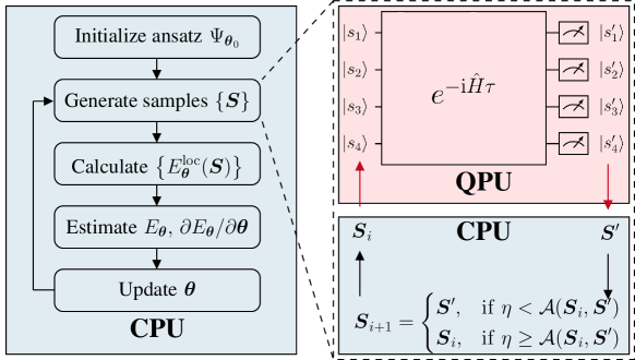
Figure 1: Flowchart of the QA-VMC algorithm. The red box highlights the quantum step excuted on quantum processor units (QPU), where a quantum time-evolution governed by a chosen Hamiltonian $\hat{H}$ satisfying $\hat{H}^{T}=\hat{H}$ and measurements are employed to propose new configurations. All other parts of the algorithm are executed on classical computers. The acceptance probability $\mathcal{A}(\bm{S}_{i},\bm{S}_{j})$ is determined by Eq. (14), and $\eta\in[0,1]$ is a uniformly distributed random number.

To gain a deeper understanding of the Quantum proposal, we decompose the corresponding proposal probability $\mathcal{Q}^{\mathrm{q}}(\bm{S}_{i},\bm{S}_{j};x_{e},\tau)$ into two parts

$$\mathcal{Q}^{\mathrm{q}}(\bm{S}_{i},\bm{S}_{j};x_{e},\tau) = \lvert\langle\bm{S}_{j}\lvert\exp(-\mathbbm{i}\hat{H}(x_{e})\tau)\lvert\bm{S}_{i}\rangle\lvert^{2}$$ (15)

$$= \sum_{n}p_{n}(\bm{S}_{i};x_{e})p_{n}(\bm{S}_{j};x_{e})+\Omega(\bm{S}_{i},\bm{S}_{j};x_{e},\tau),$$

where $p_{n}(\bm{S}_{i};x_{e})=\lvert\langle\bm{S}_{i}\lvert\Psi_{n}\rangle\lvert^{2}$ and $\{\lvert\Psi_{n}\rangle\}$ represents the eigenstates of $\hat{H}(x_{e})$, and $\Omega(\bm{S}_{i},\bm{S}_{j};x_{e},\tau)$ is given by

$$\Omega(\bm{S}_{i},\bm{S}_{j};x_{e},\tau)=2\Re{\sum_{n>m}\langle\bm{S}_{j}\lvert\Psi_{n}\rangle\langle\Psi_{n}\lvert\bm{S}_{i}\rangle\langle\bm{S}_{i}\lvert\Psi_{m}\rangle\langle\Psi_{m}\lvert\bm{S}_{j}\rangle e^{\mathbbm{i}(E_{m}-E_{n})\tau}}.$$ (16)

The first term in Eq. (15) is time-independent and will be referred to as the Effective proposal

$$\mathcal{Q}^{\mathrm{eff}}(\bm{S}_{i},\bm{S}_{j};x_{e})=\sum_{n}p_{n}(\bm{S}_{i};x_{e})p_{n}(\bm{S}_{j};x_{e}),$$ (17)

since it can be verified that $\sum_{\bm{S}_{j}}\mathcal{Q}^{\mathrm{eff}}(\bm{S}_{i},\bm{S}_{j};x_{e})=1$. While $\mathcal{Q}^{\mathrm{eff}}(\bm{S}_{i},\bm{S}_{j};x_{e})$ is inefficient to implement on classical computers and quantum computers directly, it provides valuable insights into the usefulness of the Quantum proposal based on the following observations:

First, for a Hamiltonian $\hat{H}(x_{e})$ without degeneracy, the time-averaged $\mathcal{Q}^{\mathrm{q}}$ over $\tau\in(-\infty,+\infty)$ equals $\mathcal{Q}^{\mathrm{eff}}$, i.e.,

$$\mathcal{Q}^{\mathrm{eff}}(\bm{S}_{i},\bm{S}_{j};x_{e})=\lim_{\tau\rightarrow+\infty}\frac{1}{2\tau}\int_{-\tau}^{+\tau}\mathcal{Q}^{\mathrm{q}}(\bm{S}_{i},\bm{S}_{j};x_{e},\tau^{\prime})\mathrm{d}\tau^{\prime}.$$ (18)

This implies that if we randomly select $\tau$ within some sufficiently large interval $(-T,+T)$, the averaged $\mathcal{Q}^{\mathrm{q}}$ will equal $\mathcal{Q}^{\mathrm{eff}}$. This point is further illustrated in Supporting Information for different model systems.

Second, the proposed move using $\mathcal{Q}^{\mathrm{eff}}$ has a more intuitive interpretation, because Eq. (17) can be understood as follows: given a configuration $\bm{S}_{i}$, first randomly select an eigenstate $\left|\Psi_{n}\right\rangle$ according to the conditional probability distribution $P(n|\bm{S}_{i})\equiv p_{n}(\bm{S}_{i};x_{e})$, and then randomly select a configuration $\bm{S}_{j}$ based on the conditional probability distribution $P(\bm{S}_{j}|n)\equiv p_{n}(\bm{S}_{j};x_{e})$. Thus, if $p_{0}(\bm{S}_{i})$ and $p_{0}(\bm{S}_{j})$ for the ground state are both large, $Q^{\mathrm{eff}}(\bm{S}_{i},\bm{S}_{j};x_{e})$ will also be large, regardless of the Hamming distance between $\bm{S}_{i}$ and $\bm{S}_{j}$. This suggests that for a ground state probability distribution concentrated on some configurations with large Hamming distances, the Effective proposal can offer a significant advantage over classical proposals. Based on Eq. (18), we expect the Quantum proposal to exhibit similar behavior.

A primary objective of this work is to examine whether the QA-VMC algorithm can potentially enhance the convergence of MCMC simulations, thereby providing computational efficiency gains for VMC. To investigate this, we apply this algorithm to two representative systems, i.e., FHMs and hydrogen chains, across various parameter ranges and system sizes. Through a comprehensive comparative analysis with conventional classical proposals, we evaluate the performance of QA-VMC from multiple perspectives, as detailed in the following section.

2.4 Figures of merit

2.4.1 Absolute spectral gap

The convergence rate of the Markov chain can be quantitatively characterized by its mixing time^{27, 51} $t_{\mathrm{mix}}(\varepsilon)$, which is the minimum number of steps $t$ required for the Markov chain to converge to its stationary distribution within a predefined tolerance threshold $\varepsilon$, i.e.,

$$t_{\mathrm{mix}}(\varepsilon):=\min\{t:\max_{\bm{S}_{i}}\lVert\mathcal{P}^{t}(\bm{S}_{i},\cdot)-\pi(\cdot)\lVert_{\mathrm{TV}}\leq\varepsilon\},$$ (19)

where $\lVert\cdot\lVert_{\mathrm{TV}}$ denotes the total variation distance²⁷, quantifying the discrepancy between the chain’s distribution after $t$ steps and the stationary distribution. While the exact computation of $t_{\mathrm{mix}}(\varepsilon)$ is generally intractable, it can be effectively bounded by the absolute spectral gap $\delta$ via²⁷

$$(\delta^{-1}-1)\ln{\Big{(}\frac{1}{2\varepsilon}\Big{)}}\leq t_{\mathrm{mix}}(\varepsilon)\leq\delta^{-1}\ln{\Big{(}\frac{1}{\varepsilon\min_{\bm{S}}\pi(\bm{S})}\Big{)}}.$$ (20)

Here, $\delta=1-|\lambda_{2}|\in[0,1]$ is the difference between the absolute values of the two largest eigenvalues ($\lambda_{1}=1$ and $\lambda_{2}$) of the transition matrix $\mathcal{P}$ (9), which can be computed through matrix diagonalization, making $\delta$ more readily accessible than the mixing time. As evident from Eq.(20), the spectral gap $\delta$ exhibits an inverse relationship with the bounds of the mixing time, thereby serving as a precise quantitative measure for assessing Markov chain convergence⁵¹. Specifically, a larger spectral gap $\delta$ implies smaller $t_{\mathrm{mix}}(\varepsilon)$ and hence faster convergence to the stationary distribution. However, it is crucial to acknowledge that the practical computation of $\delta$ is limited by the exponential growth of the Hilbert space. Therefore, in this work we employ an extrapolation approach adopted in the QeMCMC work⁵¹ to establish a relationship between $\delta$ and system size $N$ obtained from computationally feasible systems. This enables us to estimate the asymptotic behavior of $\delta$ for larger systems that are infeasible for diagonalization.

2.4.2 Autocorrelation time

Apart from the absolute spectral gap, autocorrelation time is another valuable metric for assessing the convergence of MCMC algorithms⁶⁶. This metric is widely used in practice because it directly captures the convergence behavior of the Markov chain, particularly in terms of how long the chain retains memory of its previous states. For a given operator $\hat{O}$, the integrated autocorrelation time $\tau_{O}$ is defined as

$$\tau_{O}=1+2\sum_{\tau=1}^{\infty}\rho_{O}(\tau),\quad\rho_{O}(\tau)=\frac{c_{O}(\tau)}{c_{O}(0)},$$ (21)

where $c_{O}(\tau)$ represents the autocovariance function at lag $\tau$

$$c_{O}(\tau)=\frac{\sum_{i=1}^{N_{s}-\tau}(O_{\mathrm{loc}}(\bm{S}_{i})-\mu_{O})(O_{\mathrm{loc}}(\bm{S}_{i+\tau})-\mu_{O})}{N_{s}-\tau}.$$ (22)

Here, $O_{\mathrm{loc}}(\bm{S}_{i})\equiv\frac{\langle\bm{S}_{i}\lvert\hat{O}\lvert\Psi\rangle}{\langle\bm{S}_{i}\lvert\Psi\rangle}$, $\mu_{O}=\frac{1}{N_{s}}\sum_{i=1}^{N_{s}}O_{\mathrm{loc}}(\bm{S}_{i})$ denotes the sample average, and $N_{s}$ represents the sample size. A smaller $\tau_{O}$ indicates faster convergence of the estimator to its mean, reflecting efficient mixing of the chain. Conversely, a larger $\tau_{O}$ suggests strong correlations among samples and slow mixing. The integrated autocorrelation time is related to the effective sample size $N_{\mathrm{eff}}$ by $N_{\mathrm{eff}}=N_{s}/\tau_{O}$. Thus, it can serve as a practical and intuitive measure of the chain’s convergence properties. We used the algorithm introduced in Ref. ⁶⁶ to estimate $\tau_{O}$.

2.4.3 Metric for potential quantum speedup

To explore the potential quantum speedup of the Quantum proposal compared to classical proposals, we analyze the asymptotic behavior of the quantity $\mathcal{T}_{\mathrm{eff}}=\delta^{-1}t_{s}$, which will be referred to as the effective runtime. Here, $\delta^{-1}$ estimates the number of steps required to reach equilibrium, and $t_{s}$ is the runtime of a single execution of a classical or quantum move. Thus, $\mathcal{T}_{\mathrm{eff}}$ roughly estimates the runtime of an ideal MCMC algorithm. The spectral gap $\delta$ can be modeled by an exponential function with respect to the system size $N$ via $\delta(N)=a2^{-kN}$⁵¹. Then, the ratio between the effective runtime of a classical proposal $\mathcal{T}_{\mathrm{eff},c}$ and that of the Quantum proposal $\mathcal{T}_{\mathrm{eff},q}$ proposals can be expressed as

$$\frac{\mathcal{T}_{\mathrm{eff},c}}{\mathcal{T}_{\mathrm{eff},q}}=\frac{\delta_{c}^{-1}t_{s,c}}{\delta_{q}^{-1}t_{s,q}}=\frac{a_{q}t_{s,c}}{a_{c}t_{s,q}}2^{(k_{c}-k_{q})N}.$$ (23)

The runtime $t_{s,c}$ for classical moves considered in this work scales at most polynomially with the system size $N$. Consequently, if the runtime $t_{s,q}$ for the quantum case also scales polynomially, then $\mathcal{T}_{\mathrm{eff},c}>\mathcal{T}_{\mathrm{eff},q}$ for sufficiently large systems, provided that $k_{c}>k_{q}$. However, if $t_{s,q}$ scales exponentially as $O(2^{bN})$, a potential speedup can only exist if $k_{c}>k_{q}+b$. Therefore, in addition to the asymptotic behavior of $\delta$ characterized by the exponent $k$, the potential quantum advantage is also critically dependent on the scaling of $t_{s,q}$ with respect to $N$. In the following sections, we will focus on the asymptotic behaviors of both $\delta$ and $t_{s,q}$.

3 Results and discussion

3.1 Fermi-Hubbard model

We begin by evaluating the performance of the QA-VMC algorithm for the FHM⁶⁷, which serves as a benchmark for both classical and quantum variational methods ^{68, 69}. The Hamiltonian of the FHM is given by:

$$\hat{H}(U)=-t\sum_{\langle i,j\rangle}\sum_{\sigma}(\hat{a}_{i\sigma}^{\dagger}\hat{a}_{j\sigma}+\mathrm{h.c.})+U\sum_{i}\hat{n}_{i\alpha}\hat{n}_{i\beta}$$ (24)

where the hopping parameter $t=1$, $U$ is the on-site interaction, $\sigma\in\{\alpha,\beta\}$, $\hat{a}_{q}^{(\dagger)}$ represent Fermionic annihilation (creation) operators, and $\langle i,j\rangle$ represents the summation over nearest-neighbor sites. Additionally, we use the Jordan-Wigner mapping⁷⁰ to transform the Fermionic Hamiltonian $\hat{H}$ into a qubit Hamiltonian expressed as a linear combination of Pauli terms, i.e. $\hat{H}=\sum_{k}h_{k}P_{k}$ with $P_{k}\in\{I,X,Y,Z\}^{\otimes N}$, and the occupation number vectors into corresponding qubit configurations. In this study, we focus on the ground state of the FHM with open boundary condition (OBC) at half-filling. In addition to the aforementioned classical proposals, we also extend the ExcitationSD proposal by incorporating a global spin flip operation, denoted by ExcitationSD+flip. In this proposal, with equal probability, either a random single/double excitation or a global spin flip is performed.

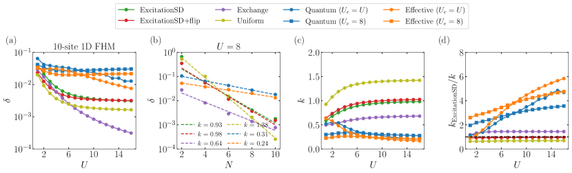
Figure 2: The absolute spectral gap $\delta$ obtained by diagonalizing the transition matrix $\mathcal{P}$ of each proposal for the ground state of the 1D FHM. For the Quantum proposal, $\delta$ is obtained as the maximal absolute spectral gap by scanning $\tau$ from $0.1$ to $20$ with a step size of $0.2$. (a) Illustration for $\delta$ of different proposals as a function of $U$ for the $10$-site 1D FHM. (b) $\delta$ of different proposals as a function of the system size $N$ for $U=8$. The function $a2^{-kN}$ is used to fit the data of each proposal, and the dashed lines are the fitted curves with the obtained $k$ shown in the inset. (c) The fitted exponent $k$ as a function of $U$. (d) $k_{\mathrm{rel}}=k_{\mathrm{ExcitationSD}}/k$ as a function of the parameter $U$. The black dashed line represents $k_{\mathrm{rel}}=1.0$.

We first analyze the asymptotic behavior for the absolute spectral gaps with the system size $N$ and the on-site interaction $U$ for the exact ground state of the one-dimensional (1D) FHM. For the Quantum proposal, $\delta$ is a function of the evolution time $\tau$. As shown in Supporting Information, as $\tau$ increases, $\delta$ first reaches that of the Effective proposal, denoted by $\delta_{\mathrm{eff}}$, and then oscillates around it. To examine the best performance that the Quantum proposal can achieve, we take the maximal absolute spectral gap by scanning $\tau$ from $0.1$ to $20$ with a step size of $0.2$ for each $U$ and $N$. The results obtained with different proposals are summarized in Figure 2, where we also plot the results obtained by the Quantum proposal with a fixed $U_{e}=8$ for all $U$. Figure 2(a) indicates that the Quantum ($U_{e}=U$) proposal and that with a fixed $U_{e}=8$ generally exhibit larger spectral gaps $\delta$ than classical proposals for $U\in[1,16]$, and behave similarly to the corresponding Effective proposals. Notably, around $U=8$, $\delta$ of the Quantum ($U_{e}=U$) proposal is approximately an order of magnitude larger than that of the ExcitationSD proposal in the 10-site 1D FHM. However, as $U$ increases to infinity, while the absolute spectral gaps of the ExcitationSD, ExcitationSD+flip, and Uniform proposals approach a fixed value, those of the Quantum ($U_{e}=U$), Effective ($U_{e}=U$), and Exchange proposals decrease. This is because in the $U=\infty$ limit, Markov chains generated by these proposals become reducible. Using a fixed $U_{e}=8$ in the Quantum proposal can avoid this problem, leading to a steady $\delta$ over a wider range of $U$.

Figure 2(b) demonstrates that $\delta$ for a fixed value of $U$ exhibits an exponential decay with increasing system size $N$ for all proposals. Following the approach outlined in Ref. ⁵¹, we fit the data using $\delta(N)=a2^{-kN}$. Note that both the prefactor $a$ and the exponent $k$ depend on $U$. The Quantum ($U_{e}=U$) and Effective ($U_{e}=U$) proposals are found to have the smallest exponents at $U=8$. Figure 2(c) presents the obtained exponents $k$ for different $U$ using the same fitting procedure, and Figure 2(d) illustrates the relative performance by plotting the ratio $k_{\mathrm{ExcitationSD}}/k$. We find that for small $U$ ($\approx 1$), the Quantum ($U_{e}=U$) proposal does not provide advantage over classical proposals. However, it does exhibit an advantage for larger $U$, indicating the potential for quantum speedup. In comparison, the Quantum approach with a fixed $U_{e}=8$ shows a more balanced performance across all $U$ values. As shown in Supporting Information, the advantage of the Quantum proposal in the exponent over classical proposals persist for 2D and random FHMs.

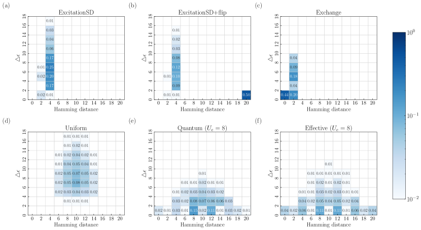
Figure 3: Comparison of different proposal probabilities $\mathcal{Q}(\bm{S_{i}},\cdot)$ from the qubit configuration $\bm{S}_{i}=(-1,1,1,-1,\cdots,-1,1,1,-1)$ with the largest ground-state probability in the $10$-site 1D FHM with $U=8$. (a)-(f) Two-dimensional histogram of $\mathcal{Q}(\bm{S_{i}},\cdot)$ with the Hamming distance (between $\bm{S}_{j}$ and $\bm{S}_{i}$) and the ’energy’ gap ($\triangle\epsilon=\mathrm{log}_{10}(P(\bm{S}_{i})/P(\bm{S}_{j}))$ as the $x$ and $y$ axes, respectively. (a) ExcitationSD. (b) ExcitationSD+flip. (c) Exchange. (d) Uniform. (e) Quantum ($U_{e}=8$). (f) Effective ($U_{e}=8$).

To understand how the Quantum proposal speeds up the convergence of the MCMC sampling at larger $U$, we introduce the configuration ’energy’ defined by

$$\epsilon(\bm{S})=-\log_{10}P(\bm{S}),\quad P(\bm{S})=|\langle\bm{S}|\Psi_{0}\rangle|^{2},$$ (25)

which is analogous to the energy function in the classical Boltzmann distribution. Specifically, a configuration with high energy $\epsilon(\bm{S})$ corresponds to a low probability $P(\bm{S})$, and a large increase in energy

$$\Delta\epsilon=\epsilon(\bm{S}_{j})-\epsilon(\bm{S}_{i})=\log_{10}(P(\bm{S}_{i})/P(\bm{S}_{j}))$$ (26)

will lead to a low acceptance rate in MCMC sampling. In Figure 3, we plot the two-dimensional histogram of different proposal probabilities $\mathcal{Q}(\bm{S_{i}},\cdot)$ for the $10$-site 1D FHM with $U=8$, with the Hamming distance and ’energy’ change $\triangle\epsilon$ as the $x$ and $y$ axes, respectively. Here, the qubit configuration $\bm{S}_{i}=(-1,1,1,-1,\cdots,-1,1,1,-1)$ is one of the two configurations with the largest ground-state probability (see Supporting Information). Its spin-flipped counterpart $(1,-1,-1,1,\dots,1,-1,-1,1)$ has an identical probability due to spin-flip symmetry ($[\hat{H},\hat{U}_{\mathrm{SF}}]=0$, where $\hat{U}_{\mathrm{SF}}=e^{\mathrm{i}\pi(\hat{S}_{x}-\hat{N}/2)}$), but the largest Hamming distance ($=20$) from $\bm{S}_{i}$. As shown in Figures 3(a)-(c), the ExcitationSD, ExcitationSD+flip, and Exchange proposals generate configurations that move only by specific Hamming distances. Moreover, the newly generated configurations often exhibit a significant increase in ’energy’, leading to a reduced acceptance rate in MCMC sampling. Figure 3(d) shows that although the Uniform proposal allows transitions over unrestricted Hamming distances, it predominantly generates high-energy configurations, thereby also decreasing the MCMC acceptance rate. In contrast, Figures 3(e) and (f) demonstrate that the Quantum and Effective proposals can generate configurations with a range of Hamming distances while maintaining relatively low ’energy’. This distinctive property significantly enhances Markov chain convergence, differentiating quantum moves from classical moves.

As discussed in the previous section, it is also crucial to examine the asymptotic behavior of the runtime $t_{s,q}$ in order to assess whether the Quantum proposal can achieve a quantum advantage in computational time. The runtime $t_{s,q}$ of a single quantum move is proportional to the evolution time $\tau$. Here, we consider the evolution time required to first reach a certain fraction of $\delta_{\mathrm{eff}}$ and analyze its dependence on the system size. This is motivated by the observation that as the evolution time increases, the spectral gap of the Quantum proposal oscillates around $\delta_{\mathrm{eff}}$ (see Supporting Information for details). Figure 4 shows the evolution time $\tau$ at which $\delta$ of the Quantum proposals ($U_{e}=U$ and $U_{e}=8$) first exceeds $c\delta_{\mathrm{eff}}$ for $c=0.6$, 0.7, and 0.8, respectively. Notably, the required evolution time does not increase rapidly with system size. In particular, it reaches a plateau for both $U=4$ and $U=8$. Similar behaviors are also observed for 2D FHMs shown in Supporting Information. Based on Eq. (23), these findings suggest that the Quantum proposal, with an appropriately chosen parameter $U_{e}$, may offer a potential quantum speedup over classical proposals for sufficiently large systems.

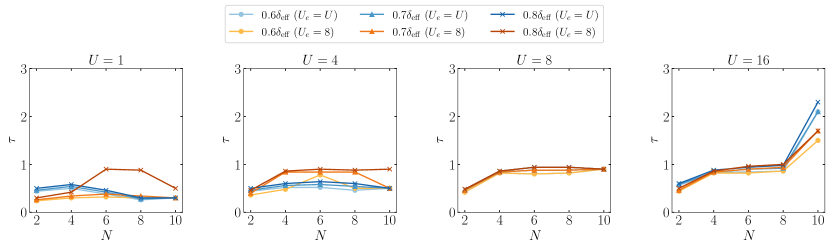
Figure 4: The evolution time $\tau$ required for $\delta$ of the Quantum proposal to first exceeds $c\delta^{\mathrm{eff}}$ ($c=0.6$, 0.7, and 0.8) as a function of the system size $N$ for the ground state of 1D FHMs with different $U$.

To further assess the quality of samples generated by different proposals, we evaluate an observable $\langle\hat{n}_{1\alpha}\hat{n}_{N\beta}\rangle$ using the MCMC algorithm for the exact ground state of the 10-site 1D FHM with $U=8$. Figure 5(a) presents the results of 100 independent Markov chains for each proposal. The Quantum proposal demonstrates superior performance, yielding more accurate results with smaller variations for a given sample size $N_{s}$. Compared to the best classical proposal (ExcitationSD+flip) for this observable, the Quantum proposal reduces the maximum error and standard deviation by approximately a factor of 3 for $N_{s}=10^{5}$, as shown in Figures 5(b) and (c). This improvement suggests that the effective sample size $N_{\mathrm{eff}}$ is roughly 9 times larger, which aligns well with the estimated integrated autocorrelation time $\tau_{n_{1\alpha}n_{N\beta}}$ for $N=10$ depicted in Figure 5(d). We extend the same analysis to other system sizes and fit the obtained $\tau_{n_{1\alpha}n_{N\beta}}$ as a function of $N$ using $a2^{kN}$ in Figure 5(d). The results reveal that the Quantum proposal exhibits the smallest $k$, and hence the slowest increase in $\tau_{n_{1\alpha}n_{N\beta}}$ as the system size $N$ increases, which is consistent with the trend observed for the absolute spectral gap. This further underscores the higher quality of samples produced by the Quantum proposal.

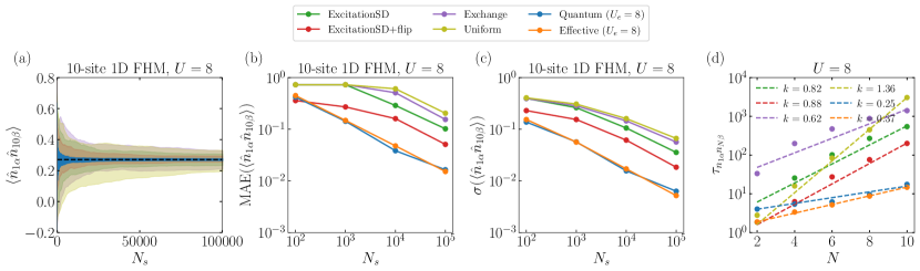
Figure 5: Estimation of an observable $\langle\hat{n}_{1\alpha}\hat{n}_{N\beta}\rangle$ by 100 independent Markov chains with different proposals for the exact ground state of 1D FHM with $U=8$. (a) The distribution of the estimated $\langle\hat{n}_{1\alpha}\hat{n}_{10\beta}\rangle$ for a given $N_{s}$ with different proposals. The black dashed line represents the exact value. (b) maximum absolute errors (MAE) for the estimated $\langle\hat{n}_{1\alpha}\hat{n}_{10\beta}\rangle$ as a function of $N_{s}$. (c) standard deviation $\sigma$ for the estimated $\langle\hat{n}_{1\alpha}\hat{n}_{10\beta}\rangle$ as a function of $N_{s}$. (d) Estimated $\tau_{n_{1\alpha}n_{10\beta}}$ as a function of $N$ for different proposals using the MCMC algorithm with $N_{s}=10^{7}$. The data were further fitted using $a2^{kN}$ (dashed lines) with the obtained exponents shown in the inset.

Finally, we illustrate the performance of the QA-VMC algorithm in practical applications by combining it with the RBM ansatz ($\alpha=3$) to target the ground-state of the 10-site 1D FHM with $U=8$. The results obtained using two different sample sizes ($N_{s}=10^{4}$ and $N_{s}=10^{5}$) are presented in Figure 6. Figure 6(a) and (b) demonstrate that the variational energy computed by QA-VMC converges more efficiently toward the exact ground-state energy, requiring fewer samples $N_{s}$ compared with classical proposals. Specifically, VMC with classical proposals fail to converge to the correct ground state using $N_{s}=10^{4}$. In contrast, the convergence trajectory of QA-VMC aligns more closely with the optimization using the exact gradients (black lines), highlighting its superior efficiency due to the higher quality of samples. Additionally, Figure 6(c) and (d) display the estimated $\langle\hat{n}_{1\alpha}\hat{n}_{10\beta}\rangle$ during the VMC optimizations. The results obtained with the Quantum proposals are found to exhibit better accuracy and smaller oscillations at the same sample size $N_{s}$ compared with classical proposals. This shows the potential of QA-VMC for significantly enhancing the performance of the VMC algorithm for large systems.

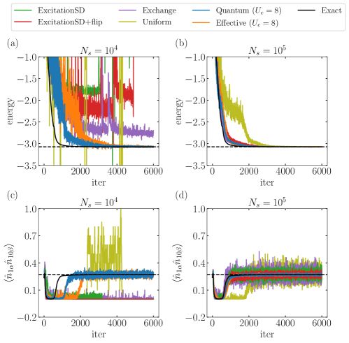
Figure 6: The VMC optimization process of different proposals using the RBM ($\alpha=3$) ansatz for 10-site 1D FHM with $U=8$. (a),(b) energy, (c),(d) $\langle\hat{n}_{1\alpha}\hat{n}_{10\beta}\rangle$. Black solid lines in (a) and (b) represent the optimization trajectory using the exact gradients without sampling. Black dashed lines represent the exact ground-state energy in (a) and (b) or $\langle\hat{n}_{1\alpha}\hat{n}_{10\beta}\rangle$ for the exact ground state in (c) and (d).

3.2 Hydrogen chains

After benchmarking QA-VMC for FHMs across various system sizes and interaction parameters, we now apply it to chemical systems with more realistic interactions. A typical example, closely related to FHMs, is the hydrogen chains at varying interatomic distances $R$, which can undergo transitions from weakly correlated systems at small $R$ to strongly correlated systems at larger $R$. The Hamiltonian for hydrogen chains employed in this work can be expressed as

$$\hat{H}(R)=\sum_{\begin{subarray}{c}pq,\sigma\end{subarray}}h_{pq}(R)\hat{a}_{p\sigma}^{\dagger}\hat{a}_{q\sigma}+\frac{1}{2}\sum_{\begin{subarray}{c}pqrs,\sigma\tau\end{subarray}}g_{pqrs}(R)\hat{a}_{p\sigma}^{\dagger}\hat{a}_{r\tau}^{\dagger}\hat{a}_{s\tau}\hat{a}_{q\sigma}+E_{\mathrm{nuc}}(R),$$ (27)

where $h_{pq}$ and $g_{pqrs}$ are molecular integrals in the orthonormalized atomic orbitals (OAO) using a STO-3G basis. The Fermionic Hamiltonian is then transformed into a qubit Hamiltonian via the Jordan-Wigner mapping⁷⁰ for subsequent studies.

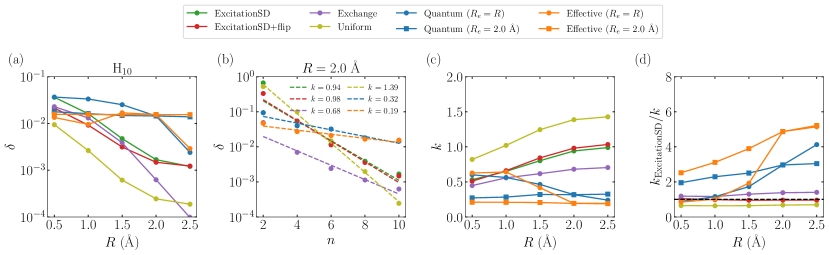
Figure 7: The absolute spectral gap $\delta$ obtained by diagonalizing the transition matrix $\mathcal{P}$ of each proposal for the ground state of the hydrogen chains H_n. For the Quantum proposal, $\delta$ is obtained as the maximal absolute spectral gap by scanning $\tau$ from $0.1$ to $60.0$ with a step size of $0.2$. (a) $\delta$ of different proposals as a function of $R$ for H10. (b) $\delta$ of different proposals as a function of the system size $n$ at $R=2.0$ Å. The function $a2^{-kN}$ is used to fit the data of each proposal, and the dashed lines are the fitted curves with the obtained $k$ shown in the inset. (c) The fitted exponent $k$ as a function of $R$. (d) $k_{\mathrm{rel}}=k_{\mathrm{ExcitationSD}}/k$ as a function of the parameter $U$. The black dashed line represents $k_{\mathrm{rel}}=1.0$.

Figure 7 presents the absolute spectral gaps $\delta$ obtained with different proposals for the ground state of hydrogen chains $\ce{H}_{n}$. As depicted in Figure 7(a), as the bond length $R$ increases from $0.5~\mathrm{\AA}$ to $2.5~\mathrm{\AA}$, the absolute spectral gap $\delta$ for the Quantum ($R_{e}=R$) proposal is generally much greater than those of classical proposals. Similar to FHMs in the large $U$ limit, $\delta$ for the Exchange, Quantum $(R_{e}=R)$, and Effective $(R_{e}=R)$ proposals decreases to zero as $R$ increases, due to the lost of irreducibility for the generated Markov chains in the $R=\infty$ limit. In contrast, other proposals maintain a nonzero $\delta$ at large $R$. In particular, by fixing $R_{e}$ to a specific value, such as 2.0 Å, the spectral gap of the Quantum proposal can sustain a large value across different $R$, see Figure 7(a). Figure 7(b) shows that $\delta$ decays exponentially with system size and is well-fitted by the function $a2^{-kN}$. At $R=2.0~\mathrm{\AA}$, the fitted exponent $k$ for the Quantum proposal is only about one-third of that of the widely used ExcitationSD proposal, indicating a significant potential speedup for large systems. Figure 7(c) and (d) display the fitted exponents $k$ for different bond lengths and the relative exponents $k_{\mathrm{rel}}=k_{\mathrm{ExcitationSD}}/k$ compared against that of ExcitationSD, respectively. It is evident that at larger $R>1.5~\mathrm{\AA}$, where the ground-state configurations become more concentrated on some configurations separated by large Hamming distances (see Supporting Information), the Quantum proposals start to outperform classical proposals.

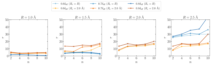
Figure 8: The evolution time $\tau$ required for $\delta$ of the Quantum proposal to first exceeds $c\delta^{\mathrm{eff}}$ ($c=0.6$, 0.7, and 0.8) as a function of the system size $n$ for the ground state of hydrogen chains H_n with different interatomic distance $R$.

In Figure 8, we further investigate the required evolution time $\tau$ for the Quantum ($R_{e}=R$ and fixed $R_{e}=2.0~\mathrm{\AA}$) proposals applied to hydrogen chains at various bond lengths. Detailed results for the absolute spectral gaps $\delta$ as a function of $\tau$ are provided in Supporting Information. As illustrated in Figure 8, the time at which $\delta$ first exceeds $c\delta_{\mathrm{eff}}$ (with $c=0.6$, 0.7, and 0.8) increases slowly with system size, particularly for the Quantum proposal with a fixed $R_{e}$. Considering both the asymptotic behaviors of the absolute spectral gap and the required evolution time, we can conclude that the Quantum $(R_{e}=2.0\,\mathrm{\AA})$ proposal has the potential to deliver an enhancement for the MCMC algorithm over classical proposals for large systems.

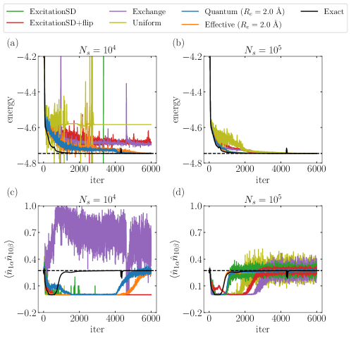
Figure 9: The VMC optimization process of different proposals using the RBM ($\alpha=3$) ansatz for the hydrogen chain H10 with $R=2.0$ Å. (a),(b) energy, (c),(d) $\langle\hat{n}_{1\alpha}\hat{n}_{10\beta}\rangle$. Black solid lines in (a) and (b) represent the optimization trajectory using the exact gradient without sampling. Black dashed lines represent the exact ground-state energy in (a) and (b) or $\langle\hat{n}_{1\alpha}\hat{n}_{10\beta}\rangle$ for the exact ground state in (c) and (d).

Finally, we illustrate the performance of QA-VMC combined with the RBM ansatz ($\alpha=3$) for computing the ground state of the hydrogen chain $\ce{H_{10}}$ and the observable $\langle\hat{n}_{1\alpha}\hat{n}_{10\beta}\rangle$ at $R=2\,\mathrm{\AA}$. The estimated energy and $\langle\hat{n}_{1\alpha}\hat{n}_{10\beta}\rangle$ during the optimization process are shown in Figure 9 for two different sample sizes, $N_{s}=10^{4}$ and $N_{s}=10^{5}$. For small $N_{s}$, Figure 9(a) and (c) reveal that the Quantum proposal significantly outperforms classical proposals. Similar to the case for FHMs, VMC with classical proposals all fail to converge to the correct ground state and $\langle\hat{n}_{1\alpha}\hat{n}_{10\beta}\rangle$ for $N_{s}=10^{4}$. Only when $N_{s}$ is increased to $10^{5}$, classical proposals begin to converge to the correct results. These results are consistent with the findings for FHMs, and underscore the potential of QA-VMC to accelerate VMC for molecular systems.

4 Conclusion

In this work, inspired by the QeMCMC algorithm⁵¹, originally designed for sampling classical Boltzmann distributions of spin models, we introduced the QA-VMC algorithm for solving the ground state of quantum many-body problems by leveraging the capabilities of quantum computers to enhance the sampling efficiency in VMC simulations. Pilot applications to FHMs and hydrogen chains reveal that the Quantum proposal exhibits larger absolute spectral gaps and reduced autocorrelation times compared to classical proposals, leading to more efficient sampling and faster convergence to the ground state in VMC. This advantage is found to be especially pronounced for specific parameter ranges, where the ground-state configurations are concentrated in some dominant configurations separated by large Hamming distances. Besides, we also identified limitations of the introduced Quantum proposal, particularly when the system parameters approach some extreme values, leading to reducible Markov chains and vanishing absolute spectral gaps. To mitigate these issues, we proposed fixing certain parameters in the Hamiltonian used for time evolution in the Quantum proposal, which can maintain a non-zero absolute spectral gap and exhibit advantages over classical proposals across a wider range of system parameters and sizes. Our results suggest that QA-VMC has the potential to enhance the performance of VMC algorithms for large systems. Future work will focus on further optimizing the Quantum proposal, including the automatic optimization of the evolution time, the use of Trotter decomposition, and investigating the algorithm’s performance on noisy quantum simulators and real quantum hardware. Additionally, exploring the application of QA-VMC to other quantum systems with more complex Hamiltonians will be crucial for assessing its broader applicability and potential for quantum advantage.

We acknowledge helpful discussions with Ming Gong. This work was supported by the Innovation Program for Quantum Science and Technology (Grant No. 2023ZD0300200) and the Fundamental Research Funds for the Central Universities.

Time-averaged Quantum proposal versus Effective proposal, the absolute spectral gap of the Quantum proposal as a function of the evolution time, exact ground state distributions of the investigated models, and additional results for 2D and random Fermi-Hubbard models.

References

- Martin et al. 2016 Martin, R. M.; Reining, L.; Ceperley, D. M. Interacting Electrons: Theory and Computational Approaches; Cambridge University Press: Cambridge, 2016
- Hohenberg and Kohn 1964 Hohenberg, P.; Kohn, W. Inhomogeneous Electron Gas. Phys. Rev. 1964, 136, B864–B871
- Kohn and Sham 1965 Kohn, W.; Sham, L. J. Self-Consistent Equations Including Exchange and Correlation Effects. Phys. Rev. 1965, 140, A1133–A1138
- Runge and Gross 1984 Runge, E.; Gross, E. K. U. Density-Functional Theory for Time-Dependent Systems. Phys. Rev. Lett. 1984, 52, 997–1000
- Čížek 1966 Čížek, J. On the Correlation Problem in Atomic and Molecular Systems. Calculation of Wavefunction Components in Ursell‐Type Expansion Using Quantum‐Field Theoretical Methods. J. Chem. Phys. 1966, 45, 4256–4266
- Purvis and Bartlett 1982 Purvis, G. D., III; Bartlett, R. J. A full coupled‐cluster singles and doubles model: The inclusion of disconnected triples. J. Chem. Phys. 1982, 76, 1910–1918
- Crawford and Schaefer III 2007 Crawford, T. D.; Schaefer III, H. F. An introduction to coupled cluster theory for computational chemists. Rev. Comput. Chem. 2007, 14, 33–136
- Shavitt and Bartlett 2009 Shavitt, I.; Bartlett, R. J. Many-Body Methods in Chemistry and Physics: MBPT and Coupled-Cluster Theory; Cambridge Molecular Science; Cambridge University Press: Cambridge, 2009
- White 1992 White, S. R. Density matrix formulation for quantum renormalization groups. Phys. Rev. Lett. 1992, 69, 2863–2866
- Chan and Sharma 2011 Chan, G. K.-L.; Sharma, S. The Density Matrix Renormalization Group in Quantum Chemistry. Annu. Rev. Phys. Chem. 2011, 62, 465–481
- Ceperley and Alder 1980 Ceperley, D. M.; Alder, B. J. Ground State of the Electron Gas by a Stochastic Method. Phys. Rev. Lett. 1980, 45, 566–569
- Zhang et al. 1997 Zhang, S.; Carlson, J.; Gubernatis, J. E. Constrained path Monte Carlo method for fermion ground states. Phys. Rev. B 1997, 55, 7464–7477
- Booth et al. 2009 Booth, G. H.; Thom, A. J. W.; Alavi, A. Fermion Monte Carlo without fixed nodes: A game of life, death, and annihilation in Slater determinant space. J. Chem. Phys. 2009, 131, 054106
- Carleo and Troyer 2017 Carleo, G.; Troyer, M. Solving the quantum many-body problem with artificial neural networks. Science 2017, 355, 602–606
- Hermann et al. 2020 Hermann, J.; Schätzle, Z.; Noé, F. Deep-neural-network solution of the electronic Schrödinger equation. Nat. Chem. 2020, 12, 891–897
- McMillan 1965 McMillan, W. L. Ground state of liquid He 4. Phys. Rev. 1965, 138, A442
- Le Roux and Bengio 2008 Le Roux, N.; Bengio, Y. Representational Power of Restricted Boltzmann Machines and Deep Belief Networks. Neural Comput. 2008, 20, 1631–1649
- Yang et al. 2020 Yang, L.; Leng, Z.; Yu, G.; Patel, A.; Hu, W.-J.; Pu, H. Deep learning-enhanced variational Monte Carlo method for quantum many-body physics. Phys. Rev. Res. 2020, 2, 012039
- Wang et al. 2024 Wang, J.-Q.; Wu, H.-Q.; He, R.-Q.; Lu, Z.-Y. Variational optimization of the amplitude of neural-network quantum many-body ground states. Phys. Rev. B 2024, 109, 245120
- Hibat-Allah et al. 2020 Hibat-Allah, M.; Ganahl, M.; Hayward, L. E.; Melko, R. G.; Carrasquilla, J. Recurrent neural network wave functions. Phys. Rev. Res. 2020, 2, 023358
- Barrett et al. 2022 Barrett, T. D.; Malyshev, A.; Lvovsky, A. I. Autoregressive neural-network wavefunctions for ab initio quantum chemistry. Nat. Mach. Intell. 2022, 4, 351–358
- Wu et al. 2023 Wu, D.; Rossi, R.; Vicentini, F.; Carleo, G. From tensor-network quantum states to tensorial recurrent neural networks. Phys. Rev. Res. 2023, 5, L032001
- Wu et al. 2023 Wu, Y.; Guo, C.; Fan, Y.; Zhou, P.; Shang, H. NNQS-transformer: an efficient and scalable neural network quantum states approach for ab initio quantum chemistry. Proceedings of the International Conference for High Performance Computing, Networking, Storage and Analysis. 2023; pp 1–13
- Viteritti et al. 2023 Viteritti, L. L.; Rende, R.; Becca, F. Transformer Variational Wave Functions for Frustrated Quantum Spin Systems. Phys. Rev. Lett. 2023, 130, 236401
- Cao et al. 2024 Cao, X.; Zhong, Z.; Lu, Y. Vision Transformer Neural Quantum States for Impurity Models. arXiv preprint arXiv:2408.13050 2024,
- Hermann et al. 2023 Hermann, J.; Spencer, J.; Choo, K.; Mezzacapo, A.; Foulkes, W. M. C.; Pfau, D.; Carleo, G.; Noé, F. Ab initio quantum chemistry with neural-network wavefunctions. Nature Reviews Chemistry 2023, 7, 692–709
- Levin and Peres 2017 Levin, D.; Peres, Y. Markov Chains and Mixing Times; American Mathematical Society: Providence, Rhode Island, 2017
- Wolff 1990 Wolff, U. Critical slowing down. Nucl. Phys. B Proc. Suppl. 1990, 17, 93–102
- Jiang et al. 2024 Jiang, T.; Zhang, J.; Baumgarten, M. K.; Chen, M.-F.; Dinh, H. Q.; Ganeshram, A.; Maskara, N.; Ni, A.; Lee, J. Walking through Hilbert space with quantum computers. arXiv preprint arXiv:2407.11672 2024,
- Arute et al. 2019 Arute, F. et al. Quantum supremacy using a programmable superconducting processor. Nature 2019, 574, 505–510
- Wu et al. 2021 Wu, Y. et al. Strong Quantum Computational Advantage Using a Superconducting Quantum Processor. Phys. Rev. Lett. 2021, 127, 180501
- Cao et al. 2019 Cao, Y.; Romero, J.; Olson, J. P.; Degroote, M.; Johnson, P. D.; Kieferová, M.; Kivlichan, I. D.; Menke, T.; Peropadre, B.; Sawaya, N. P. D.; Sim, S.; Veis, L.; Aspuru-Guzik, A. Quantum Chemistry in the Age of Quantum Computing. Chem. Rev. 2019, 119, 10856–10915
- McArdle et al. 2020 McArdle, S.; Endo, S.; Aspuru-Guzik, A.; Benjamin, S. C.; Yuan, X. Quantum computational chemistry. Rev. Mod. Phys. 2020, 92, 015003
- Bauer et al. 2020 Bauer, B.; Bravyi, S.; Motta, M.; Chan, G. K.-L. Quantum Algorithms for Quantum Chemistry and Quantum Materials Science. Chem. Rev. 2020, 120, 12685–12717
- Motta and Rice 2022 Motta, M.; Rice, J. E. Emerging quantum computing algorithms for quantum chemistry. WIREs Comput. Mol. Sci. 2022, 12, e1580
- Szegedy 2004 Szegedy, M. Quantum speed-up of Markov chain based algorithms. 45th Annual IEEE Symposium on Foundations of Computer Science. 2004; pp 32–41
- Somma et al. 2008 Somma, R. D.; Boixo, S.; Barnum, H.; Knill, E. Quantum Simulations of Classical Annealing Processes. Phys. Rev. Lett. 2008, 101, 130504
- Wocjan and Abeyesinghe 2008 Wocjan, P.; Abeyesinghe, A. Speedup via quantum sampling. Phys. Rev. A 2008, 78, 042336
- Poulin and Wocjan 2009 Poulin, D.; Wocjan, P. Sampling from the Thermal Quantum Gibbs State and Evaluating Partition Functions with a Quantum Computer. Phys. Rev. Lett. 2009, 103, 220502
- Bilgin and Boixo 2010 Bilgin, E.; Boixo, S. Preparing Thermal States of Quantum Systems by Dimension Reduction. Phys. Rev. Lett. 2010, 105, 170405
- Temme et al. 2011 Temme, K.; Osborne, T. J.; Vollbrecht, K. G.; Poulin, D.; Verstraete, F. Quantum Metropolis sampling. Nature 2011, 471, 87–90
- Yung and Aspuru-Guzik 2012 Yung, M.-H.; Aspuru-Guzik, A. A quantum–quantum Metropolis algorithm. Proc. Natl Acad. Sci. USA 2012, 109, 754–759
- Montanaro 2015 Montanaro, A. Quantum speedup of Monte Carlo methods. Proc. R. Soc. A 2015, 471, 20150301
- Chowdhury and Somma 2017 Chowdhury, A. N.; Somma, R. D. Quantum algorithms for Gibbs sampling and hitting-time estimation. Quantum Inf. Comput. 2017, 17, 41–64
- Lemieux et al. 2020 Lemieux, J.; Heim, B.; Poulin, D.; Svore, K.; Troyer, M. Efficient Quantum Walk Circuits for Metropolis-Hastings Algorithm. Quantum 2020, 4, 287
- Arunachalam et al. 2022 Arunachalam, S.; Havlicek, V.; Nannicini, G.; Temme, K.; Wocjan, P. Simpler (classical) and faster (quantum) algorithms for Gibbs partition functions. Quantum 2022, 6, 789
- Rall et al. 2023 Rall, P.; Wang, C.; Wocjan, P. Thermal State Preparation via Rounding Promises. Quantum 2023, 7, 1132
- Chen et al. 2023 Chen, C.-F.; Kastoryano, M. J.; Gilyén, A. An efficient and exact noncommutative quantum Gibbs sampler. arXiv preprint arXiv:2311.09207 2023,
- Wild et al. 2021 Wild, D. S.; Sels, D.; Pichler, H.; Zanoci, C.; Lukin, M. D. Quantum Sampling Algorithms for Near-Term Devices. Phys. Rev. Lett. 2021, 127, 100504
- Wild et al. 2021 Wild, D. S.; Sels, D.; Pichler, H.; Zanoci, C.; Lukin, M. D. Quantum sampling algorithms, phase transitions, and computational complexity. Phys. Rev. A 2021, 104, 032602
- Layden et al. 2023 Layden, D.; Mazzola, G.; Mishmash, R. V.; Motta, M.; Wocjan, P.; Kim, J.-S.; Sheldon, S. Quantum-enhanced Markov chain Monte Carlo. Nature 2023, 619, 282–287
- Nakano et al. 2024 Nakano, Y.; Hakoshima, H.; Mitarai, K.; Fujii, K. Markov-chain Monte Carlo method enhanced by a quantum alternating operator ansatz. Phys. Rev. Res. 2024, 6, 033105
- Ding et al. 2024 Ding, Z.; Chen, C.-F.; Lin, L. Single-ancilla ground state preparation via Lindbladians. Phys. Rev. Res. 2024, 6, 033147
- Orfi and Sels 2024 Orfi, A.; Sels, D. Bounding the speedup of the quantum-enhanced Markov-chain Monte Carlo algorithm. Phys. Rev. A 2024, 110, 052414
- Orfi and Sels 2024 Orfi, A.; Sels, D. Barriers to efficient mixing of quantum-enhanced Markov chains. Phys. Rev. A 2024, 110, 052434
- Christmann et al. 2024 Christmann, J.; Ivashkov, P.; Chiurco, M.; Mazzola, G. From quantum enhanced to quantum inspired Monte Carlo. arXiv preprint arXiv:2411.17821 2024,
- Lockwood et al. 2024 Lockwood, O.; Weiss, P.; Aronshtein, F.; Verdon, G. Quantum dynamical Hamiltonian Monte Carlo. Phys. Rev. Res. 2024, 6, 033142
- Ferguson and Wallden 2024 Ferguson, S.; Wallden, P. Quantum-enhanced Markov Chain Monte Carlo for systems larger than your Quantum Computer. arXiv preprint arXiv:2405.04247 2024,
- Sajjan et al. 2024 Sajjan, M.; Singh, V.; Kais, S. Polynomially efficient quantum enabled variational Monte Carlo for training neural-network quantum states for physico-chemical applications. arXiv preprint arXiv:2412.12398 2024,
- Sorella 2005 Sorella, S. Wave function optimization in the variational Monte Carlo method. Phys. Rev. B 2005, 71, 241103
- Pfau et al. 2020 Pfau, D.; Spencer, J. S.; Matthews, A. G. D. G.; Foulkes, W. M. C. Ab initio solution of the many-electron Schrödinger equation with deep neural networks. Phys. Rev. Res. 2020, 2, 033429
- Choo et al. 2020 Choo, K.; Mezzacapo, A.; Carleo, G. Fermionic neural-network states for ab-initio electronic structure. Nat. Commun. 2020, 11, 2368
- Torlai et al. 2018 Torlai, G.; Mazzola, G.; Carrasquilla, J.; Troyer, M.; Melko, R.; Carleo, G. Neural-network quantum state tomography. Nat. Phys. 2018, 14, 447–450
- Kingma 2014 Kingma, D. P. Adam: A method for stochastic optimization. arXiv preprint arXiv:1412.6980 2014,
- Metropolis et al. 1953 Metropolis, N.; Rosenbluth, A. W.; Rosenbluth, M. N.; Teller, A. H.; Teller, E. Equation of State Calculations by Fast Computing Machines. J. Chem. Phys. 1953, 21, 1087–1092
- Sokal 1997 Sokal, A. In Functional Integration: Basics and Applications; DeWitt-Morette, C., Cartier, P., Folacci, A., Eds.; Springer US: Boston, MA, 1997; pp 131–192
- Arovas et al. 2022 Arovas, D. P.; Berg, E.; Kivelson, S. A.; Raghu, S. The Hubbard Model. Annu. Rev. Condens. Matter Phys. 2022, 13, 239–274
- Yokoyama and Shiba 1987 Yokoyama, H.; Shiba, H. Variational Monte-Carlo Studies of Hubbard Model. I. J. Phys. Soc. Jpn. 1987, 56, 1490–1506
- Cade et al. 2020 Cade, C.; Mineh, L.; Montanaro, A.; Stanisic, S. Strategies for solving the Fermi-Hubbard model on near-term quantum computers. Phys. Rev. B 2020, 102, 235122
- Jordan and Wigner 1928 Jordan, P.; Wigner, E. P. About the Pauli exclusion principle. Z. Phys 1928, 47, 14–75