Towards Ultimate NMR Resolution with
Deep Learning
Abstract
In multidimensional NMR spectroscopy, practical resolution is defined as the ability to distinguish and accurately determine signal positions against a background of overlapping peaks, thermal noise, and spectral artifacts. In the pursuit of ultimate resolution, we introduce Peak Probability Presentations ()—a statistical spectral representation that assigns a probability to each spectral point, indicating the likelihood of a peak maximum occurring at that location. The mapping between the spectrum and is achieved using MR-Ai, a physics-inspired deep learning neural network architecture, designed to handle multidimensional NMR spectra. Furthermore, we demonstrate that MR-Ai enables co-processing of multiple spectra, facilitating direct information exchange between datasets. This feature significantly enhances spectral quality, particularly in cases of highly sparse sampling. Performance of MR-Ai and high value of the are demonstrated on the synthetic data and spectra of Tau, MATL1, Calmodulin, and several other proteins.
Keywords Nuclear magnetic resonance (NMR) Non-uniform sampling (NUS) Deep Learning (DL) WNN Targeted Acquisition Hyper-dimensional spectroscopy
1 Introduction
NMR spectroscopy has provided increasingly valuable insights into the behavior and properties of molecules. Over the past decades, it has established itself as an essential atomic-level tool in structural biology [1] and has played a crucial role in protein structural analysis [2]. Despite its versatility, NMR spectroscopy of biological systems is often constrained by limited spectral resolution, where signal overlap complicates chemical shift assignment and interferes with the analysis of molecular dynamics and structure [3]. Since the introduction of Fourier NMR spectroscopy in the middle of 1960s [4], numerous signal processing methods have been developed and are now routinely used to enhance resolution. These include traditional techniques such as zero-padding [5, 6], apodization with weighting functions [7], linear prediction [8], virtual decoupling by deconvolution [9, 10, 11, 12], and, more recently, spectral signal sharpening using artificial neural networks (NNs) [13]. In response to the limitations of traditional approaches, Artificial Intelligence (AI), particularly Deep Learning (DL), has demonstrated significant potential across various areas of NMR research [14, 15, 16]. AI-based tools not only surpass traditional NMR techniques in rapid and high-quality non-uniform sampling (NUS) reconstruction [17, 18, 19, 20], efficient homonuclear decoupling [21, 20], pure shift spectra generation [22, 23, 24], spectra denoising [25, 26], and automated peak picking [27, 28], but also have the potential to push beyond the boundaries of traditional Magnetic Resonance processing, for example allowing reference-free assessment of the spectra quality and obtaining phase sensitive spectra without quadrature detection [29].
In this work, we address the challenge of achieving ultimate resolution and reducing data complexity in experimental NMR spectra affected by thermal noise, spectral artifacts, and signal overlap. Instead of relying on the relatively broad and loosely defined notion of spectral resolution, we redefine the problem in a more precise statistical framework—determining the probability of finding the center of a signal at any given point in the spectrum. This reformulation shifts the focus to statistical analysis using AI [30].
The Bayesian approach has previously been used to define posterior probability distributions of spectral parameters in 1D metabolomic spectra, leveraging a templated library of expected underlying compounds [31, 32]. However, applying traditional Bayesian methods to unconstrained multidimensional protein spectra is computationally prohibitive due to the immense processing demands associated with Markov chain Monte Carlo (MCMC) algorithms [33]. AI circumvents this computational bottleneck by exploiting the efficiency of deep learning in solving classification problems [30], enabling direct probability predictions. Reformulating the resolution problem as a classification task—peak or no peak—bridges the gap between statistical analysis and practical applications in multidimensional NMR.
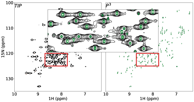
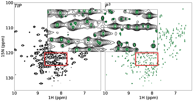
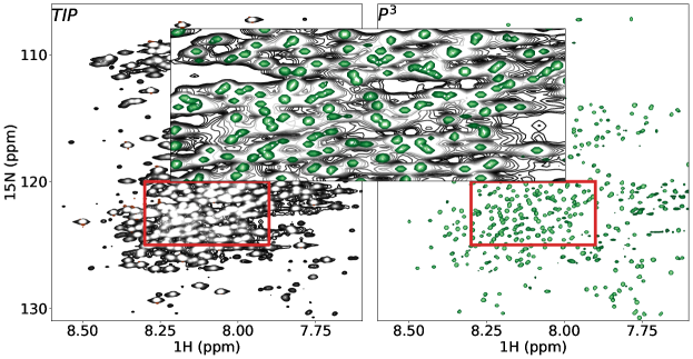
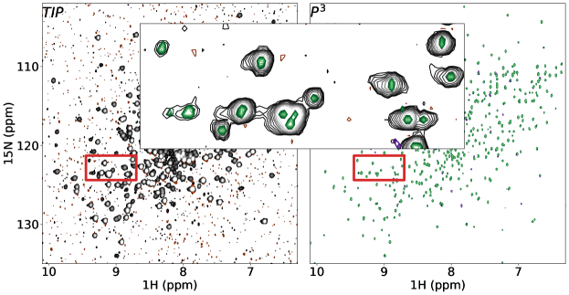
NMR spectra are commonly analyzed in the frequency domain using Traditional Intensity Presentation (TIP). While TIP is highly informative, it has notable drawbacks, including peak overlap exacerbated by the high dynamic range of signal intensities and difficulties in distinguishing genuine peaks from spectral artifacts. As a complementary alternative to TIP, we introduce Peak Probability Presentation (), a statistical representation applicable to NMR spectra of any dimensionality. assigns, to each point in the spectrum, the probability of it being a peak maximum. This approach offers several advantages, including super-resolution, high sensitivity, a significantly reduced dynamic range, and effective suppression of spectral artifacts.
Using simulated data and experimental spectra from several challenging systems including the globular MALT1 protein (45 kDa) and the intrinsically disordered Tau protein (45.8 kDa) we demonstrate that achieves near-ultimate spectral resolution based on the available information in 2D and 3D spectra. We introduce the newly developed Magnetic Resonance Processing with AI (MR-Ai) system, which is capable of handling both conventionally acquired spectra and non-uniformly sampled (NUS) data reconstructed using nonlinear compressed sensing algorithms [34, 35, 36, 37, 38, 39, 40, 41, 42, 43, 44, 45, 46]. Furthermore, using a set of triple-resonance experiments for backbone assignment collected on the Calamondin protein, we demonstrate that can serve as a spectral quality metric, similar to the number of detected peaks in Targeted Acquisition (TA) data collection schemes [47, 48].
2 Results and Discussion
2.1 Ultimate Resolution and dynamic range in :
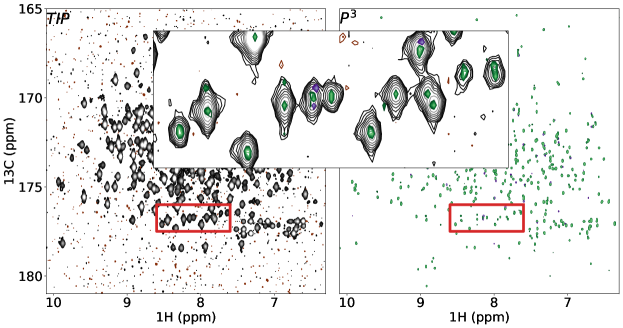
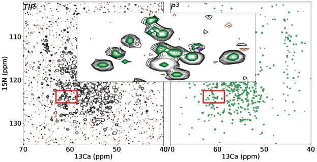
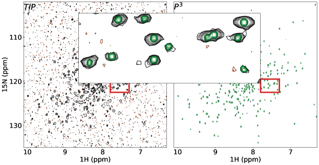
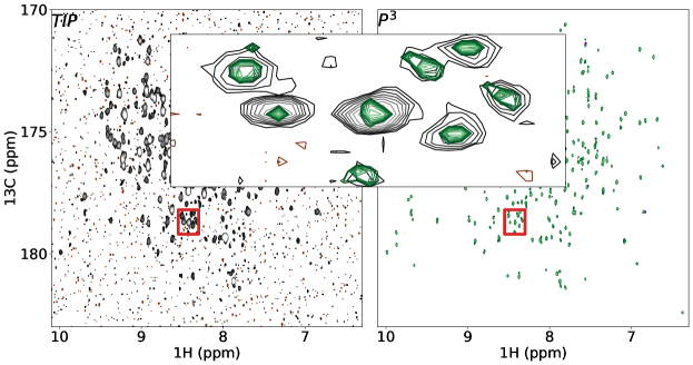
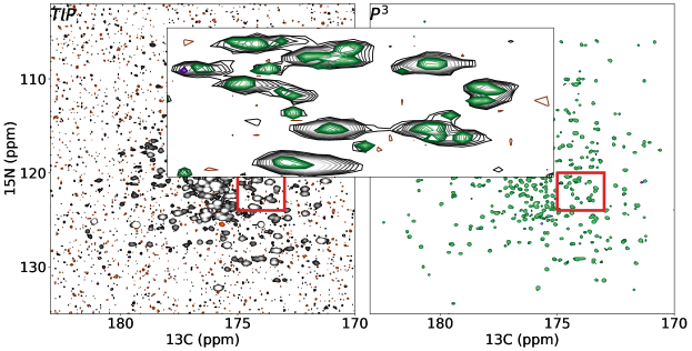
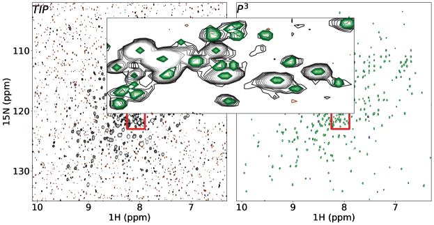
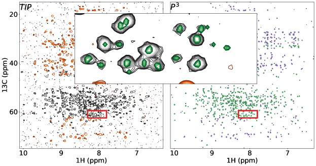
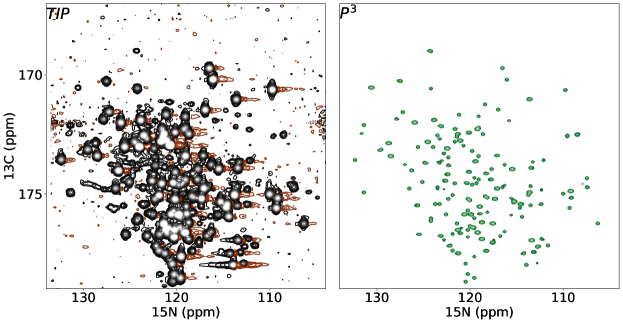
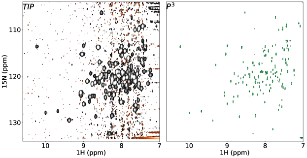
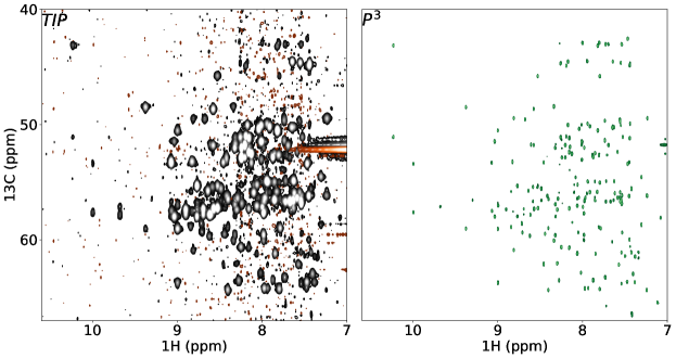
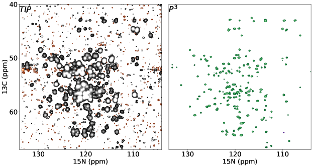
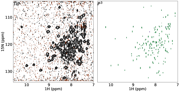
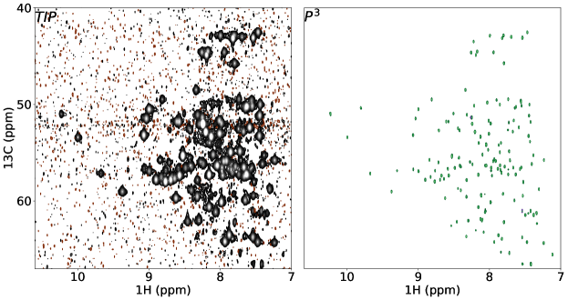
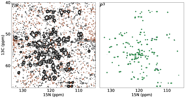
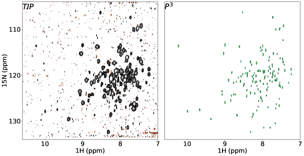
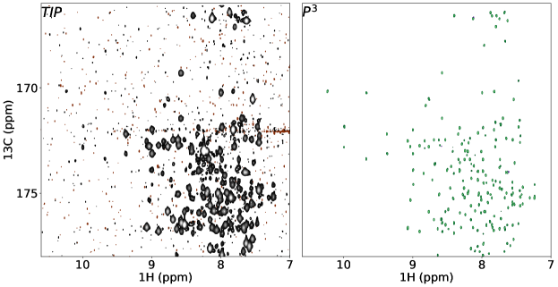
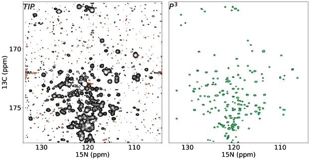
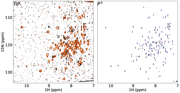
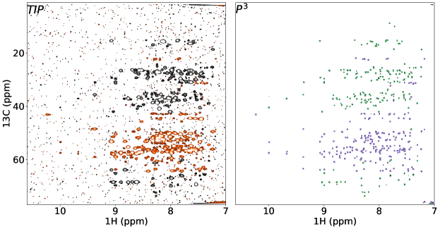
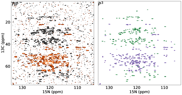
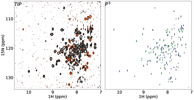
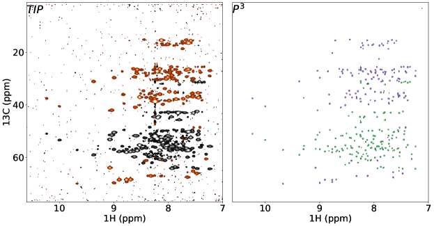
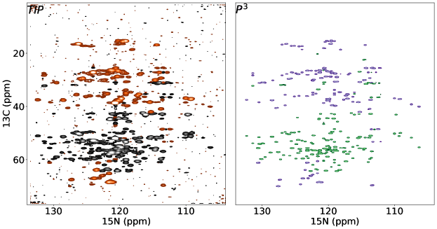
Figure 1 demonstrates the excellent performance of MR-Ai in generating for the 2D 1H-15N correlation spectrum of MALT1 protein (45 kDa) [49, 50]. Similar results for Ubiquitin (7 kDa) [51], Azurin (14 kDa) [52], and Tau (disordered, 45.8 kDa) [53] are provided in Supplementary Figures S1, S2, and S3, respectively.
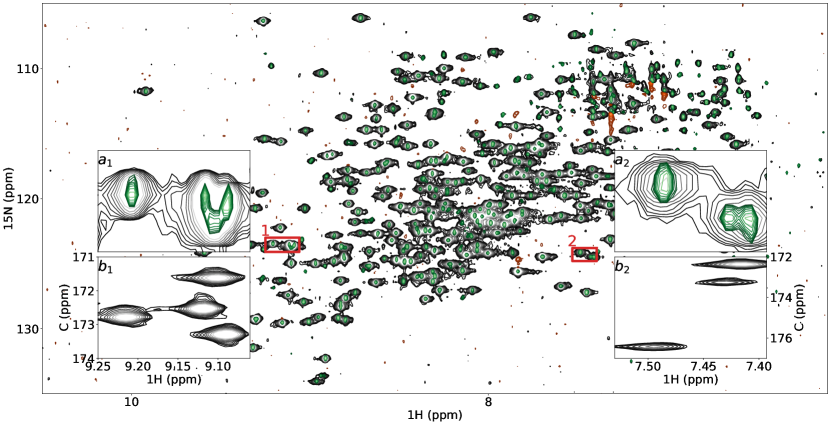
The representation exhibits significant line narrowing across the 2D spectrum while accurately reproducing both strong and weak peaks. The two insets in Figure 1 confirm the improved resolution by displaying the peaks resolved in alongside the corresponding 1H-13C slice from the 3D HNCO spectrum.
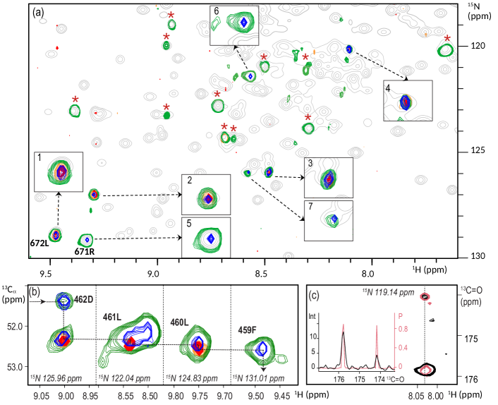
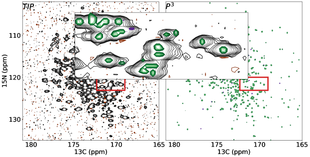
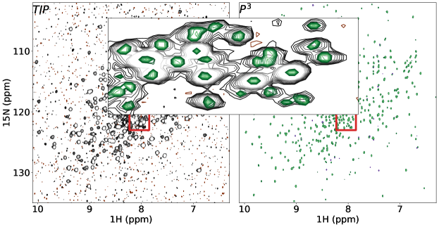
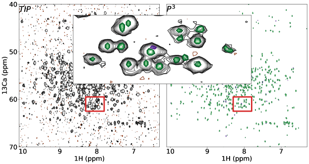
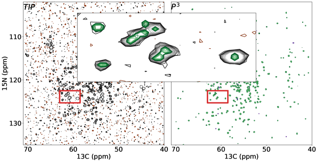
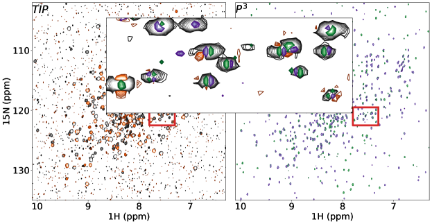
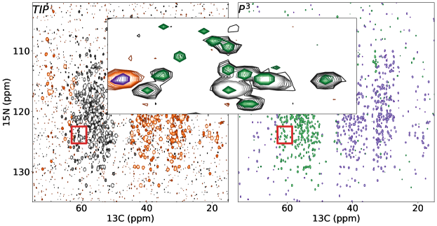
Figure 2 illustrates the application of to the backbone assignment of the 45 kDa MALT1 protein using 3D HNCA and HN(CO)CA spectra. The assignment progresses from residue to its preceding residue through visual inspection of the 1H-15N 2D planes extracted from the two 3D spectra at 13C: 55.01 ppm, corresponding to the 13C frequency of . In the crowded spectra of MALT1, this assignment is significantly complicated by the presence of multiple candidate cross-peaks for . Figure 2a shows numerous cross-peaks in HNCA (green contours) and HN(CO)CA (orange contours), all of which must be carefully evaluated to establish the correct sequential connection. The ambiguity, arising from insufficient resolution in the 13C dimension of traditional spectra, is largely alleviated in the representation (Figure 2a, blue for HNCA and red for HN(CO)CA). The enhanced resolution eliminates most of the irrelevant peaks (marked by red stars). Among the remaining seven peaks, only peak 5 (the correct peak) and peaks 6 and 7 are retained in the of the HNCA spectrum.
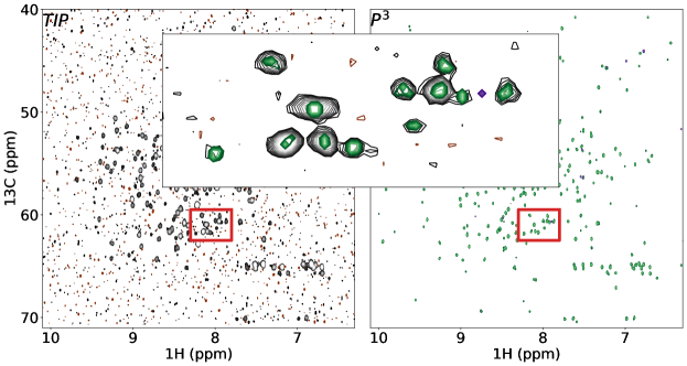
Another example of the superior resolution along the 1H and 13C dimensions in the representation of the MALT1 3D HNCA and HN(CO)CA spectra is shown in Figure 2b. This figure illustrates the assignment walk from to , tracing to cross-peaks in four 1H-13C 2D strips extracted at 15N: 125.96, 122.04, 124.83, and 131.01 ppm, respectively. The assignment walk is particularly challenging when relying solely on traditional 3D HNCA (green contours) and HN(CO)CA (orange contours) spectra, often necessitating additional experiments. In contrast, the walk based on better resolved , shown in blue (HNCA) and red (HN(CO)CA), is highly reliable, offering improved confidence in peak identification.
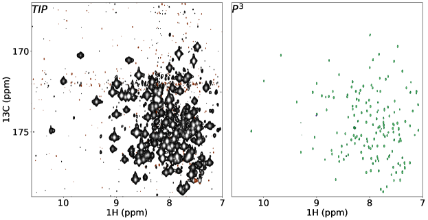
A remarkable difference in signal dynamic range between the traditional intensity presentation and is illustrated in Figure 2c, which shows a 2D strip extracted from the 3D HN(CA)CO spectrum for residue at 15N: 119.14 ppm. Two cross-peaks, observed at 174.07 ppm and 175.87 ppm, correspond to the carbonyl 13C frequencies of and , respectively. A 1D slice taken through these two cross-peaks at 1H: 8.038 ppm reveals a significant difference in the relative peak amplitudes. In the representation, both peaks exhibit high and nearly equal probability (about 0.8), whereas in the conventional spectrum, their amplitude ratio is 3:1. Notably, in 3D HN(CA)CO spectrum, optimized for detecting 1H-15N-13C(i) cross-peaks corresponding to a residue’s own carbonyl carbon, the second peak, which corresponds to the carbonyl of the preceding residue, typically has lower intensity or may even disappear. The ability to simultaneously visualize all reliably detected signals, regardless of their intensity, significantly simplifies manual spectral analysis.
2.2 Validation of the on synthetic spectra
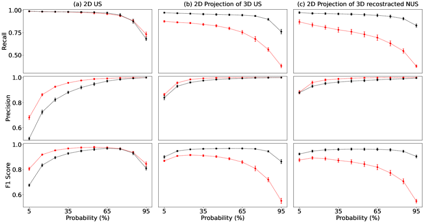
Despite the promising results obtained for the spectra of MALT1, Ubiquitin, Azurin, and Tau proteins, quantitatively assessing the performance of using experimental data remains challenging due to the absence of ground truth peak labeling. To address this limitation, we evaluated using synthetic spectra. Figure 3 presents the recall and precision metrics [54] of , calculated across ten 2D and ten 3D synthetic spectra. Each spectrum contains 256 peaks with varying degrees of overlap and amplitudes, spanning a dynamic range of 1:200, with the weakest peaks reaching one -noise. In all cases, including fully sampled 2D and 3D spectra as well as 3D NUS spectra, a favorable balance is observed between the number of spectral points correctly and incorrectly assigned to peak maxima. Thus, around a shallow optimum at approximately 50% probability, most true peaks are accurately detected, while the false detection rate remains very low.
Although 2D spectra exhibit a significantly higher degree of peak overlap compared to 3D spectra, demonstrates remarkably consistent performance in both cases. Furthermore, as shown in Figure 3b, the quality of in 3D NUS-reconstructed spectra, which feature strongly non-Gaussian baseline noise, is comparable to that of uniformly sampled (US) data.
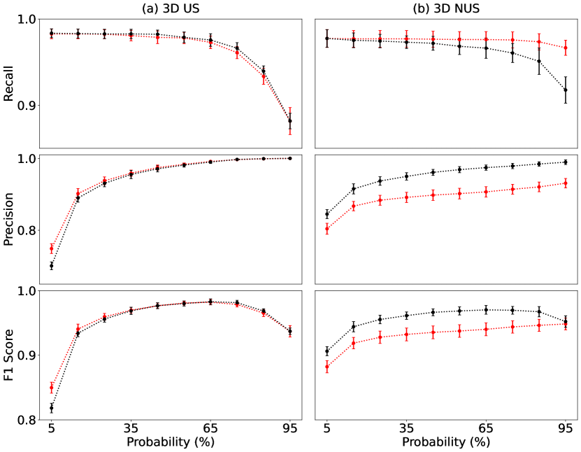
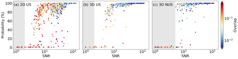
Figure 4 illustrates the range of probability values for identifying peak maxima at spectral points corresponding to ground-truth peaks in synthetic 2D and 3D spectra. The values are clearly influenced by the peak signal-to-noise ratio (SNR) and the degree of peak overlap. The latter is determined by the number of neighboring peaks, their relative distances, and their amplitudes compared to the peak in question.
In the 2D spectra (Figure 4a), peaks with have nearly zero probability values and are therefore not detected. This lower boundary for peak detection is close to the theoretical detection limit at a confidence level () and can also be attributed to the substantially higher degree of interference and overlap with other peaks, particularly for low-intensity peaks, as indicated by the color scale in Figure 4. Although most peaks with are detected with high probability, a few medium-intensity peaks exhibit reduced probability values due to significant overlap. These peaks are located at the bottom of the chart. A similar pattern, although with less pronounced overlap, is observed in both 3D uniformly sampled (US) spectra (Figure 4b) and 3D -NUS spectra (Figure 4c). A notable feature of in the -NUS 3D spectra is that the apparent peak detection threshold is very close to the theoretical limit. This highlights the near-ideal performance of both the CS-IST NUS spectrum reconstruction algorithm and the produced by MR-Ai for synthetic spectra.
The results obtained from experimental spectra of several representative proteins, supported by quantitative validation using synthetic data, establish as a powerful tool for significantly enhancing spectral resolution and simplifying analysis. Furthermore, highlights new opportunities in NMR signal processing and analysis enabled by AI-driven approaches.
2.3 Reference-Free Quantitative Spectrum Quality Score with , QSP:
In our previous work [29], we demonstrated that MR-Ai can be trained to predict intensity uncertainties in spectra reconstructed by various methods. These predicted uncertainties can serve as a reference-free score for assessing spectrum quality. In this work, we introduce the integral of as a useful proxy for the number of peaks in a spectrum. This is reminiscent of traditional 1D NMR, where the integral of the spectrum is proportional to the number of spins in the sample. We further introduce a quantitative spectrum quality score (QSP) corresponding to the number of detectable peaks, which is defined as the number of clusters of spectral points with values exceeding a defined threshold ().
2.4 Targeted Acquisition with hyper-dimensional QSP:
Targeted Acquisition (TA) is a NUS-based incremental data acquisition strategy, in which the quality of processed spectra is concurrently assessed, typically in relation to a task-specific target, such as detecting a predefined number of peaks [55]. TA provides essential feedback on experimental progress and enables timely termination of data collection, thereby significantly reducing measurement time for lengthy experiments. The key ingredient of the TA procedure is a reliable and meaningful spectrum quality score that can be calculated at different levels of data completion. In our original implementation of the TA for the protein backbone assignment, the peaks in the 3D NUS triple resonance experiments were detected at each TA step using a hyper-dimensional extension of the multi-dimensional decomposition [48, 56]. This approach was necessary to replace traditional peak-picking routines, which perform poorly on strongly under-sampled NUS spectra. However, generalizing this highly specialized and task-dependent method to other spectrum types and analysis tasks remains challenging. Leveraging ultimate resolution, high sensitivity, and accurate differentiation between genuine peaks and artifacts, and QSP provide a new, general, and reliable method for estimating the number of detectable peaks—without requiring explicit peak picking. This enables real-time assessment of spectrum quality during the TA process. As demonstrated below, also introduces a novel AI-based approach for hyper-dimensional co-processing [57, 56] of multiple spectra.
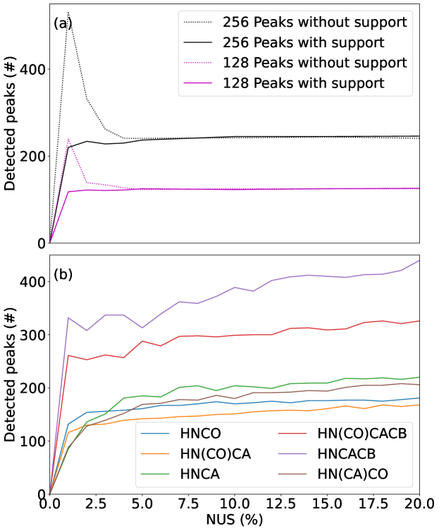
Figure 5a demonstrates that QSP can be used to quantitatively predict the number of detectable peaks in 3D spectra reconstructed with CS-IST across a wide range of NUS rates. Increasing the number of peaks in the synthetic spectra from 128 to 256 results in a corresponding doubling of the QSP score, confirming its linear response to the number of true peaks. The figure also highlights the advantage of hyper-dimensional co-processing, which is particularly beneficial at low NUS fractions. In Figure 5b, the hyper-dimensional QSP is applied to a set of experiments for backbone assignment in Calmodulin protein (16.7 kDa). The curves show a typical TA build-up of peaks, where the number of detected peaks increases as more NUS data is collected, with little further improvement beyond approximately NUS, as confirmed by visual inspection of the spectra. Notably, the plateau values of the curves correspond to the expected number of peaks for each experiment type in the protein. The TA buildup curves of peak numbers in individual 3D spectra of Calmodulin closely resemble those obtained using the original TA procedure [48] for the same spectra.
3 Conclusion
In this work, we leverage the power of AI to achieve the ultimate resolution attainable through signal processing of multidimensional NMR spectra. We introduce , a new type of statistical spectral representation designed to enhance resolution while suppressing noise and spectral artifacts. We present a novel MR-Ai architecture based on a physics-aware cross-objective framework, generalized for any dimensionality. We demonstrate the high value of for the analysis of 3D spectra from several representative globular and disordered proteins. Furthermore, we illustrate its application in hyper-dimensional spectral analysis and Targeted Acquisition.
4 Methods
4.1 MR-Ai Architecture for nD pattern:
We introduce a generalized version of our Magnetic Resonance processing with AI (MR-Ai) architecture, designed to handle NMR spectra of any dimensionality. The MR-Ai framework was originally developed [29] for capturing 2D spectral patterns, including phase-twisted peaks associated with P-type (or N-type) data in the frequency domain [29]. The original MR-Ai was, in turn, based on our earlier deep neural network architecture, WNN [20], which was designed to analyze 1D NMR frequency-domain spectra. The WNN model effectively captures defined spectral features, such as specific patterns of NUS aliasing artifacts and peak multiplicities in homonuclear decoupling experiments.
The new MR-Ai, referred to in this paper simply as MR-Ai, captures specific spectral patterns along the multidimensional cross in Cartesian coordinates, centered at a probed spectral point (Figure 6). This cross-objective representation of the nD spectrum is inspired by the physical model of the NMR signal as a tensor product of 1D shapes [34]. While notably compact, the cross-field of view retains most essential signal features, including line shape, phase distortions, -noise, -coupling multiplets, wiggles from spectral truncation, and NUS-related Point Spread Function (PSF) patterns. Using a larger field of view, for example, an nD box, would require more DNN parameters and introduce more noise than new information.
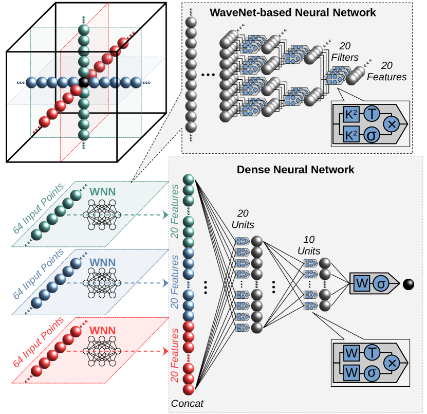
Figure 6 depicts the architecture of MR-Ai, designed for generating . Each vector within the cross-objective is first processed individually by the WNN module, which converts it into a 20-feature vector. The WNN architecture consists of 1D convolutional layers with a stride of 2, effectively skipping one data point between each convolution operation. Each layer employs a kernel size of 2 () and contains 10 filters, using a combination of hyperbolic tangent activation functions () and sigmoid activation functions (), without padding between layers. The feature vectors generated by the final WNN layers for all spectral dimensions are concatenated and passed as input into a Dense Neural Network (DNN) with two hidden layers, containing 20 and 10 units, respectively. Each hidden layer applies the same combination of hyperbolic tangent () and sigmoid () activation functions.
A crucial aspect of deep neural network design is selecting an appropriate cost function, which must align closely with the chosen output unit activation function. Both the cost function and activation function depend on the specific task. For instance, in regression problems such as NUS reconstruction, Echo reconstruction, or virtual decoupling, a Rectified Linear Unit (ReLU) activation function [58] combined with a Mean Square Error (MSE) loss function is commonly used [20]. Conversely, for uncertainty estimation, the Negative Log-Likelihood (NLL) loss function is required [29]. For , determining the probability of a peak maximum is a binary classification problem with two classes: peak maxima points labeled as 1, and all other points labeled as 0 (). In this context, the Binary Cross-Entropy (BCE) loss function, combined with a sigmoid activation function, provides an effective solution [30].
The sigmoid function converts model outputs into probabilities by mapping values to the range :
| (1) |
This property makes it ideal for binary classification tasks, where the output represents the likelihood of belonging to the peak maxima class. For a Bernoulli distribution, the probability of observing a label given a predicted probability is defined as:
| (2) |
Taking the negative of this likelihood yields the BCE loss function:
| (3) |
By minimizing BCE, the model optimizes its outputs to assign probabilities close to 1 for peak maxima and close to 0 for all other regions. This approach corresponds to maximizing the likelihood under a Bernoulli distribution. The output layer of the DNN consists of a single unit with a sigmoid activation function and uses BCE as the loss function. This layer processes the concatenated feature vectors to generate the final output, representing the adjusted probability value for the central point within the cross-objective, informed by the surrounding spectral context. The network architecture and graphs were generated using the TensorFlow Python library [59] with the Keras front-end. The model was trained within TensorFlow using the stochastic ADAM optimizer [60] with default parameters, a learning rate of 0.001, a mini-batch size of , and up to epochs. Training was terminated early if the monitored metric failed to improve on the validation dataset. MR-Ai were trained on the NMRbox server [61], equipped with 128 cores, 2 TB of memory, and 4 NVIDIA A100 Tensor Core GPUs.
4.2 Training MR-Ai model for :
The first challenge in training a deep neural network is acquiring a sufficiently large and diverse dataset. To effectively train the model, it is necessary to generate a substantial number of cross-objectives along with their corresponding labels (1 for peak maxima and 0 otherwise). This requires access to a large number of spectra with accurately annotated peak positions. Our previous studies demonstrated that synthetic data can serve as an effective proxy for realistic experimental NMR spectra [29, 20]. In this work, we train MR-Ai using synthetic spectra, generating approximately cross-objectives and their associated labels. While most previous efforts have primarily focused on signal modeling, we incorporate synthetic noise to better simulate spectra representative of real experimental conditions. We found that accurately modeling noise with an appropriate statistical distribution, as described below, is just as critical as modeling the signal itself, especially for NUS-reconstructed data, where low-intensity peaks are particularly affected.
4.2.1 Synthetic nD spectra with associated labeling
For training, nD NMR time domain a hyper-complex signal , usually called free induction decay (FID), can be presented as a superposition of a small number of exponential functions:
| (4) |
where and run over the number of exponentials and dimensions respectively where the th exponential in th dimensional has the amplitude , phase , relaxation time , frequency . The evolution time is given by the series 0, 1, …, -1, where is the number of complex points in th dimension. The desired number of different FIDs for the training and testing set is simulated by randomly varying the above parameters in the ranges summarized in Table 1 for 2D 1H-15N and 3D 1H-15N-13C correlation spectra.
| Direct | Indirect | |
|---|---|---|
| 128 | 128 | |
| [-0.5,0.5] | [-0.5,0.5] | |
| [,] | [,] | |
| [12.8,64] | [64,1280] | |
| [0.05,1] | ||
| 256 | ||
We used Python libraries, including nmrglue [62] and NMRPipe [63], for reading, writing, and processing NMR spectra, as well as mddnmr [34]. The uniformly sampled spectra were obtained with the standard nD processing steps, which included apodization, zero-filling, Fourier Transform (FT), and phase correction.
A binary label matrix, matching the dimensions of each processed synthetic spectrum, was generated based on the provided peak list. Matrix elements were assigned a value of one at indices corresponding to peak maxima and zero elsewhere. If a peak maximum fell between two data points, within a range of 0.25 to 0.75 units from each, both adjacent elements were assigned a value of one.
4.2.2 Training model for 2D US spectra:
To train the model for 2D US spectra, we generated 640 synthetic noise-free 2D US spectra (using a 4:1 ratio for training and validation datasets) based on Table 1. The noise was simulated by a random Gaussian-distributed signal in the time domain and subsequently processed to the frequency spectrum using the same procedure as for synthetic spectra. After normalization of the noise in the frequency domain, so that its standard deviation matches to the smallest possible peak amplitude, the noise was added to the synthetic spectrum, .
4.2.3 Training model for 3D spectra:
To train the model for 3D spectra, we generated 1,280 synthetic noise-free 3D US spectra based on Table 1. Groups of four spectra were added with positive and negative signs. This increased the number of peaks and overlaps as well as resulted in both positive and negative peaks. Similar to 2D US spectra, the 3D US spectra include Gaussian noise. However, in the case of 3D NUS spectra reconstructed using the CS-IST algorithm, the apparent baseline noise and artifacts do not follow a normal (Gaussian) distribution. To address this discrepancy, we empirically determined (Figure 7a) that as the number of NUS points decreases, the noise distribution shifts toward a Cauchy-like distribution.
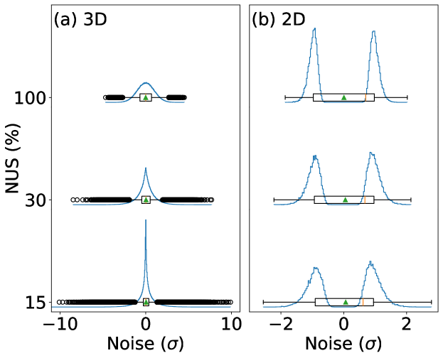
To simulate this behavior, we modeled the noise as a combination of Cauchy and Gaussian distributions, where their relative contribution varies as a function of the NUS fraction. Using Cauchy-featured noise instead of a purely Gaussian distribution during training enhanced the precision of the trained network without significantly compromising its sensitivity, as measured by the recall score (see Supplementary Figure S16). After normalizing the synthetic noise in the frequency domain, it was added to as previously described.
4.3 Resampling and the Regions of interest:
In classification tasks, an imbalance in class representation, where one class significantly outnumbers another, can lead to biased models that perform poorly on the minority class [64, 65]. In 2D spectra, where the class ratio (i.e., the number of points with and without spectral maxima) is approximately 1:100, this slight imbalance does not pose a significant issue. However, in 3D spectra, a severe imbalance arises due to the sparsity of 3D data, with class ratios exceeding . Training the deep neural network on such an imbalanced dataset results in a model that is insensitive to low-intensity peaks, creating substantial challenges during training. To mitigate this issue, resampling techniques—which adjust the training data to balance class distributions—can significantly improve model performance. These techniques include oversampling the minority class or undersampling the majority class [64, 65]. For training the model in the 3D case, we specifically under-sampled data points associated with the background. This was achieved by selecting all points corresponding to peak maxima (labels with zeros) and a subset of non-peak points (labels with zeros), ensuring a class ratio of approximately 1:100. This approach significantly improved the model’s sensitivity to small peaks but also led to an increase in false positive hits. This is unsurprising, as even in an ideal 3D spectrum of typical size filled with Gaussian noise, more than 100 peaks are expected to exhibit intensities exceeding four standard deviations of the baseline noise. The number of noise-induced peak-like features is even greater in NUS-reconstructed spectra. To mitigate this issue, we focus the analysis on regions of interest, as described below.
4.3.1 Training model for 2D Sky projections of 3D spectra:
Although the trained network for 3D spectra can successfully detect even very low SNR peaks, it is also highly sensitive to spurious peak-like noise features and spectral artifacts in NUS spectra. Distinguishing real peaks from intense noise features and artifacts is nearly impossible without additional prior knowledge.
As it was noted above, the 2D spectra do not display a significant imbalance in the representation of the classes’ peaks versus non-peak. This allows direct detection of the low-intensity peaks. Moreover, even if the baseline noise in a 3D spectrum has a strong Cauchy-like deviation from Gaussian distribution, the noise in the 2D projections has a distribution featuring favorable properties of the normal distribution due to the central limit theorem (CLT) [66]. To leverage this property, we trained models to predict values for all three 2D sky projections of the 3D spectrum. The primary difference between 2D sky projections of 3D spectra and conventional 2D uniformly sampled (US) spectra lies in their noise distributions. While noise in 2D US spectra follows a Gaussian distribution, noise in 2D sky projections from 3D spectra resembles a symmetric double Gaussian distribution. Figure 7b illustrates that across a broad range of NUS rates (–), artifacts and noise in 2D sky projections exhibit similar distributions, with slight variations in the middle gap and spread. To replicate this behavior during training, we modeled noise as a double Gaussian distribution. This approach significantly improves recall by capturing the characteristics of 2D sky projections from 3D spectra reconstructed under both US and different NUS rates (see also Supplementary Figure S15).
4.4 Production run of trained MR-Ai:
For 2D US spectra, the trained MR-Ai model, designed to handle Gaussian-distributed noise, can be applied directly to predict . In the case of 3D spectra, reconstruction is preceded by an intermediate step to identify regions of interest, as depicted in Figure 8.
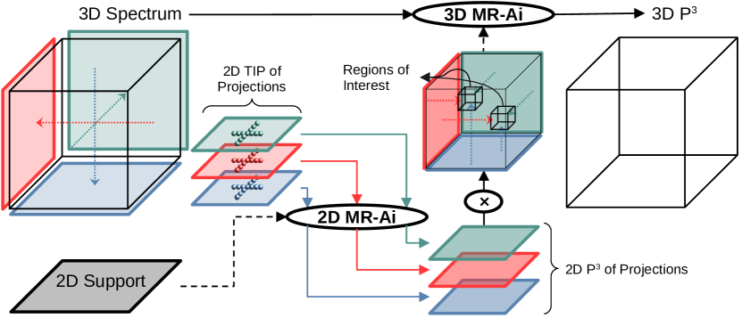
First, values are calculated for the three orthogonal 2D sky projections using an MR-Ai model trained on 2D projections with noise modeled as a double Gaussian distribution. Then, each point in the original 3D spectrum is assigned a preliminary probability score, computed as the element-wise product of the corresponding probability values from the 2D projections. Points in the 3D spectrum with a score exceeding are selected as regions of interest. This threshold corresponds to a minimum probability of approximately 2.5% in the individual 2D projections. Finally, spectral points within the regions of interest are evaluated using the sensitive 3D MR-Ai model, which was trained on noise modeled as a Cauchy-Gaussian distribution. It is worth noting that 2D projections can be directly measured in the time domain due to the Fourier Projection Theorem and have been successfully used in NMR for a long time, particularly in NUS spectrum reconstruction for multidimensional spectra [67, 68, 41].
MR-Ai enables the hyper-dimensional analysis and co-processing of multiple spectra, leveraging the power of multi-spectral integration. [57, 56, 69]. As shown in Figure 8, MR-Ai incorporates supporting spectra during the definition of regions of interest. For instance, for enhanced signal detection, an alternative high-sensitivity 2D spectrum (e.g., 2D HSQC) can be used instead of a 2D sky projection from a processed 3D spectrum. As illustrated in Figure 5a, such spectral support is particularly beneficial in the sampling-limited regime, where the number of available NUS points is too low for reliably resolving all the spectra signals.
4.5 Synthetic test data:
To test the trained MR-Ai model, we generated 2D and 3D US spectra based on Table 1 and added Gaussian-distributed noise. For the 3D NUS case, the 3D US spectrum was first down-sampled to the desired number of NUS points. Subsequently, CS-IST was used for the spectrum reconstruction.
4.6 Experimental test data:
To test trained MR-Ai performances, we used previously described 2D and 3D spectra for several proteins: Ubiquitin [51], Azurin [52], Tau (IDP) [53], MALT1 [49, 50], and Calmodulin [70]. The 2D US and 3D NUS experiments used in this study are described in Table 2. We used NMRPipe [63], Python package nmrglue [62], mddnmr [55], and TopSpin (Bruker Biospin) software for reading, writing, and traditional processing of the NMR spectra. We employed CS-IST [37], using the default mddnmr parameters and the Virtual-Echo mode [71] for 3D NUS reconstruction.
| Protein | Ubiquitin | Azurin | Tau | MALT1 | Calmodulin |
|---|---|---|---|---|---|
| Size | 8.6 kDa | 14 kDa | 45.8 kDa | 44 kDa | 17 kDa |
| Concentration | 0.6 mM | 1 mM | 0.5 mM | 0.5 mM | 1 mM |
| Spectrum | 2D US (1H, 15N) | ||||
| HSQC | HSQC | TROSY | TROSY | ||
| 3D NUS (1H, 13C,15N) | |||||
| HNCO | HNCO | ||||
| HNCA | HNCA | ||||
| HN(CA)CO | HN(CA)CO | ||||
| HN(CO)CA | HN(CO)CA | ||||
| HNCACB | HNCACB | ||||
| — | HN(CO)CACB | ||||
References
- [1] T. D. Claridge, High-resolution NMR techniques in organic chemistry, vol. 27. Elsevier, 2016.
- [2] Y. Hu, K. Cheng, L. He, X. Zhang, B. Jiang, L. Jiang, C. Li, G. Wang, Y. Yang, and M. Liu, “Nmr-based methods for protein analysis,” Analytical chemistry, vol. 93, no. 4, pp. 1866–1879, 2021.
- [3] J. Cavanagh, W. J. Fairbrother, A. G. Palmer III, and N. J. Skelton, Protein NMR spectroscopy: principles and practice. Academic press, 1996.
- [4] R. R. Ernst and W. A. Anderson, “Application of fourier transform spectroscopy to magnetic resonance,” Review of Scientific Instruments, vol. 37, no. 1, pp. 93–102, 1966.
- [5] J. C. Lindon and A. Ferrige, “Digitisation and data processing in fourier transform nmr,” Progress in Nuclear Magnetic Resonance Spectroscopy, vol. 14, no. 1, pp. 27–66, 1980.
- [6] E. Bartholdi and R. Ernst, “Fourier spectroscopy and the causality principle,” Journal of Magnetic Resonance (1969), vol. 11, no. 1, pp. 9–19, 1973.
- [7] A. Ebel, W. Dreher, and D. Leibfritz, “Effects of zero-filling and apodization on spectral integrals in discrete fourier-transform spectroscopy of noisy data,” Journal of Magnetic Resonance, vol. 182, no. 2, pp. 330–338, 2006.
- [8] H. Oschkinat, C. Griesinger, P. J. Kraulis, O. W. Sørensen, R. R. Ernst, A. M. Gronenborn, and G. M. Clore, “Three-dimensional nmr spectroscopy of a protein in solution,” Nature, vol. 332, no. 6162, pp. 374–376, 1988.
- [9] M. A. Delsuc and G. C. Levy, “The application of maximum entropy processing to the deconvolution of coupling patterns in nmr,” Journal of Magnetic Resonance (1969), vol. 76, no. 2, pp. 306–315, 1988.
- [10] N. Shimba, H. Kovacs, A. S. Stern, A. M. Nomura, I. Shimada, J. C. Hoch, C. S. Craik, and V. Dötsch, “Optimization of 13 c direct detection nmr methods,” Journal of Biomolecular NMR, vol. 30, pp. 175–179, 2004.
- [11] K. Kazimierczuk, P. Kasprzak, P. S. Georgoulia, I. Matečko-Burmann, B. M. Burmann, L. Isaksson, E. Gustavsson, S. Westenhoff, and V. Y. Orekhov, “Resolution enhancement in nmr spectra by deconvolution with compressed sensing reconstruction,” Chemical Communications, vol. 56, no. 93, pp. 14585–14588, 2020.
- [12] T. Qiu, A. Jahangiri, X. Han, D. Lesovoy, T. Agback, P. Agback, A. Achour, X. Qu, and V. Orekhov, “Resolution enhancement of nmr by decoupling with the low-rank hankel model,” Chemical Communications, vol. 59, no. 36, pp. 5475–5478, 2023.
- [13] V. K. Shukla, G. Karunanithy, P. Vallurupalli, and D. F. Hansen, “A combined nmr and deep neural network approach for enhancing the spectral resolution of aromatic side chains in proteins,” Science Advances, vol. 10, no. 51, p. eadr2155, 2024.
- [14] D. Chen, Z. Wang, D. Guo, V. Orekhov, and X. Qu, “Review and prospect: deep learning in nuclear magnetic resonance spectroscopy,” Chemistry–A European Journal, vol. 26, no. 46, pp. 10391–10401, 2020.
- [15] V. K. Shukla, G. T. Heller, and D. F. Hansen, “Biomolecular nmr spectroscopy in the era of artificial intelligence,” Structure, vol. 31, no. 11, pp. 1360–1374, 2023.
- [16] Y. Luo, X. Zheng, M. Qiu, Y. Gou, Z. Yang, X. Qu, Z. Chen, and Y. Lin, “Deep learning and its applications in nuclear magnetic resonance spectroscopy,” Progress in Nuclear Magnetic Resonance Spectroscopy, vol. 146, p. 101556, 2025.
- [17] X. Qu, Y. Huang, H. Lu, T. Qiu, D. Guo, T. Agback, V. Orekhov, and Z. Chen, “Accelerated nuclear magnetic resonance spectroscopy with deep learning,” Angewandte Chemie, vol. 132, no. 26, pp. 10383–10386, 2020.
- [18] D. F. Hansen, “Using deep neural networks to reconstruct non-uniformly sampled nmr spectra,” Journal of biomolecular NMR, vol. 73, no. 10, pp. 577–585, 2019.
- [19] G. Karunanithy and D. F. Hansen, “Fid-net: A versatile deep neural network architecture for nmr spectral reconstruction and virtual decoupling,” Journal of biomolecular NMR, vol. 75, no. 4, pp. 179–191, 2021.
- [20] A. Jahangiri, X. Han, D. Lesovoy, T. Agback, P. Agback, A. Achour, and V. Orekhov, “Nmr spectrum reconstruction as a pattern recognition problem,” Journal of Magnetic Resonance, vol. 346, p. 107342, 2023.
- [21] G. Karunanithy, H. W. Mackenzie, and D. F. Hansen, “Virtual homonuclear decoupling in direct detection nuclear magnetic resonance experiments using deep neural networks,” Journal of the American Chemical Society, vol. 143, no. 41, pp. 16935–16942, 2021.
- [22] X. Zheng, Z. Yang, C. Yang, X. Shi, Y. Luo, J. Luo, Q. Zeng, Y. Lin, and Z. Chen, “Fast acquisition of high-quality nuclear magnetic resonance pure shift spectroscopy via a deep neural network,” The Journal of Physical Chemistry Letters, vol. 13, no. 9, pp. 2101–2106, 2022.
- [23] H. Zhan, J. Liu, Q. Fang, X. Chen, Y. Ni, and L. Zhou, “Fast pure shift nmr spectroscopy using attention-assisted deep neural network,” Advanced Science, p. 2309810, 2024.
- [24] H. Zhan, J. Liu, Q. Fang, X. Chen, and L. Hu, “Accelerated pure shift nmr spectroscopy with deep learning,” Analytical Chemistry, vol. 96, no. 4, pp. 1515–1521, 2024.
- [25] H. H. Lee and H. Kim, “Intact metabolite spectrum mining by deep learning in proton magnetic resonance spectroscopy of the brain,” Magnetic resonance in medicine, vol. 82, no. 1, pp. 33–48, 2019.
- [26] D. Chen, W. Hu, H. Liu, Y. Zhou, T. Qiu, Y. Huang, Z. Wang, M. Lin, L. Lin, Z. Wu, et al., “Magnetic resonance spectroscopy deep learning denoising using few in vivo data,” IEEE Transactions on Computational Imaging, 2023.
- [27] P. Klukowski, M. Augoff, M. Zięba, M. Drwal, A. Gonczarek, and M. J. Walczak, “Nmrnet: a deep learning approach to automated peak picking of protein nmr spectra,” Bioinformatics, vol. 34, no. 15, pp. 2590–2597, 2018.
- [28] D.-W. Li, A. L. Hansen, L. Bruschweiler-Li, C. Yuan, and R. Brüschweiler, “Fundamental and practical aspects of machine learning for the peak picking of biomolecular nmr spectra,” Journal of Biomolecular NMR, pp. 1–9, 2022.
- [29] A. Jahangiri and V. Orekhov, “Beyond traditional magnetic resonance processing with artificial intelligence,” Communications Chemistry, vol. 7, no. 1, p. 244, 2024.
- [30] Y. Bengio, I. Goodfellow, and A. Courville, Deep learning, vol. 1. MIT press Cambridge, MA, USA, 2017.
- [31] W. Astle, M. De Iorio, S. Richardson, D. Stephens, and T. Ebbels, “A bayesian model of nmr spectra for the deconvolution and quantification of metabolites in complex biological mixtures,” Journal of the American Statistical Association, vol. 107, no. 500, pp. 1259–1271, 2012.
- [32] J. Hao, M. Liebeke, W. Astle, M. De Iorio, J. G. Bundy, and T. Ebbels, “Bayesian deconvolution and quantification of metabolites in complex 1d nmr spectra using batman,” Nature protocols, vol. 9, no. 6, pp. 1416–1427, 2014.
- [33] C. Andrieu, N. De Freitas, and A. Doucet, “Sequential mcmc for bayesian model selection,” in Proceedings of the IEEE Signal Processing Workshop on Higher-Order Statistics. SPW-HOS’99, pp. 130–134, IEEE, 1999.
- [34] V. Jaravine, I. Ibraghimov, and V. Yu Orekhov, “Removal of a time barrier for high-resolution multidimensional nmr spectroscopy,” Nature methods, vol. 3, no. 8, pp. 605–607, 2006.
- [35] M. Mobli and J. C. Hoch, “Nonuniform sampling and non-fourier signal processing methods in multidimensional nmr,” Progress in nuclear magnetic resonance spectroscopy, vol. 83, pp. 21–41, 2014.
- [36] X. Qu, M. Mayzel, J.-F. Cai, Z. Chen, and V. Orekhov, “Accelerated nmr spectroscopy with low-rank reconstruction,” Angewandte Chemie International Edition, vol. 54, no. 3, pp. 852–854, 2015.
- [37] K. Kazimierczuk and V. Y. Orekhov, “Accelerated nmr spectroscopy by using compressed sensing,” Angewandte Chemie, vol. 123, no. 24, pp. 5670–5673, 2011.
- [38] S. G. Hyberts, A. G. Milbradt, A. B. Wagner, H. Arthanari, and G. Wagner, “Application of iterative soft thresholding for fast reconstruction of nmr data non-uniformly sampled with multidimensional poisson gap scheduling,” Journal of biomolecular NMR, vol. 52, pp. 315–327, 2012.
- [39] H. Hassanieh, M. Mayzel, L. Shi, D. Katabi, and V. Y. Orekhov, “Fast multi-dimensional nmr acquisition and processing using the sparse fft,” Journal of Biomolecular NMR, vol. 63, pp. 9–19, 2015.
- [40] S. G. Hyberts, K. Takeuchi, and G. Wagner, “Poisson-gap sampling and forward maximum entropy reconstruction for enhancing the resolution and sensitivity of protein nmr data,” Journal of the American Chemical Society, vol. 132, no. 7, pp. 2145–2147, 2010.
- [41] Y. Pustovalova, M. Mayzel, and V. Y. Orekhov, “Xlsy: Extra-large nmr spectroscopy,” Angewandte Chemie, vol. 130, no. 43, pp. 14239–14241, 2018.
- [42] S. Sibisi, J. Skilling, R. G. Brereton, E. D. Laue, and J. Staunton, “Maximum entropy signal processing in practical nmr spectroscopy,” Nature, vol. 311, no. 5985, pp. 446–447, 1984.
- [43] I. Drori, “Fast minimization by iterative thresholding for multidimensional nmr spectroscopy,” EURASIP Journal on Advances in Signal Processing, vol. 2007, pp. 1–10, 2007.
- [44] D. J. Holland, M. J. Bostock, L. F. Gladden, and D. Nietlispach, “Fast multidimensional nmr spectroscopy using compressed sensing,” Angewandte Chemie, vol. 123, no. 29, pp. 6678–6681, 2011.
- [45] B. Jiang, X. Jiang, N. Xiao, X. Zhang, L. Jiang, X.-a. Mao, and M. Liu, “Gridding and fast fourier transformation on non-uniformly sparse sampled multidimensional nmr data,” Journal of Magnetic Resonance, vol. 204, no. 1, pp. 165–168, 2010.
- [46] J. Ying, F. Delaglio, D. A. Torchia, and A. Bax, “Sparse multidimensional iterative lineshape-enhanced (smile) reconstruction of both non-uniformly sampled and conventional nmr data,” Journal of biomolecular NMR, vol. 68, pp. 101–118, 2017.
- [47] V. A. Jaravine and V. Y. Orekhov, “Targeted acquisition for real-time nmr spectroscopy,” Journal of the American Chemical Society, vol. 128, no. 41, pp. 13421–13426, 2006.
- [48] L. Isaksson, M. Mayzel, M. Saline, A. Pedersen, J. Rosenlöw, B. Brutscher, B. G. Karlsson, and V. Y. Orekhov, “Highly efficient nmr assignment of intrinsically disordered proteins: application to b-and t cell receptor domains,” PLos one, vol. 8, no. 5, p. e62947, 2013.
- [49] S. Unnerståle, M. Nowakowski, V. Baraznenok, G. Stenberg, J. Lindberg, M. Mayzel, V. Orekhov, and T. Agback, “Backbone assignment of the malt1 paracaspase by solution nmr,” Plos one, vol. 11, no. 1, p. e0146496, 2016.
- [50] X. Han, M. Levkovets, D. Lesovoy, R. Sun, J. Wallerstein, T. Sandalova, T. Agback, A. Achour, P. Agback, and V. Y. Orekhov, “Assignment of ivl-methyl side chain of the ligand-free monomeric human malt1 paracaspase-igl3 domain in solution,” Biomolecular NMR Assignments, vol. 16, no. 2, pp. 363–371, 2022.
- [51] P. S. Brzovic, A. Lissounov, D. E. Christensen, D. W. Hoyt, and R. E. Klevit, “A ubch5/ubiquitin noncovalent complex is required for processive brca1-directed ubiquitination,” Molecular cell, vol. 21, no. 6, pp. 873–880, 2006.
- [52] D. M. Korzhnev, B. G. Karlsson, V. Y. Orekhov, and M. Billeter, “Nmr detection of multiple transitions to low-populated states in azurin,” Protein Science, vol. 12, no. 1, pp. 56–65, 2003.
- [53] D. M. Lesovoy, P. S. Georgoulia, T. Diercks, I. Matečko-Burmann, B. M. Burmann, E. V. Bocharov, W. Bermel, and V. Y. Orekhov, “Unambiguous tracking of protein phosphorylation by fast high-resolution fosy nmr,” Angewandte Chemie International Edition, vol. 60, no. 44, pp. 23540–23544, 2021.
- [54] C. Sammut and G. I. Webb, Encyclopedia of machine learning. Springer Science & Business Media, 2011.
- [55] V. Y. Orekhov and V. A. Jaravine, “Analysis of non-uniformly sampled spectra with multi-dimensional decomposition,” Progress in nuclear magnetic resonance spectroscopy, vol. 59, no. 3, pp. 271–292, 2011.
- [56] V. A. Jaravine, A. V. Zhuravleva, P. Permi, I. Ibraghimov, and V. Y. Orekhov, “Hyperdimensional nmr spectroscopy with nonlinear sampling,” Journal of the American Chemical Society, vol. 130, no. 12, pp. 3927–3936, 2008.
- [57] Ē. Kupče and R. Freeman, “Hyperdimensional nmr spectroscopy,” Journal of the American Chemical Society, vol. 128, no. 18, pp. 6020–6021, 2006.
- [58] A. Agarap, “Deep learning using rectified linear units (relu),” arXiv preprint arXiv:1803.08375, 2018.
- [59] M. Abadi, A. Agarwal, P. Barham, E. Brevdo, Z. Chen, C. Citro, G. S. Corrado, A. Davis, J. Dean, M. Devin, et al., “Tensorflow: Large-scale machine learning on heterogeneous distributed systems,” arXiv preprint arXiv:1603.04467, 2016.
- [60] D. P. Kingma, “Adam: A method for stochastic optimization,” arXiv preprint arXiv:1412.6980, 2014.
- [61] M. W. Maciejewski, A. D. Schuyler, M. R. Gryk, I. I. Moraru, P. R. Romero, E. L. Ulrich, H. R. Eghbalnia, M. Livny, F. Delaglio, and J. C. Hoch, “Nmrbox: a resource for biomolecular nmr computation,” Biophysical journal, vol. 112, no. 8, pp. 1529–1534, 2017.
- [62] J. J. Helmus and C. P. Jaroniec, “Nmrglue: an open source python package for the analysis of multidimensional nmr data,” Journal of biomolecular NMR, vol. 55, pp. 355–367, 2013.
- [63] F. Delaglio, S. Grzesiek, G. W. Vuister, G. Zhu, J. Pfeifer, and A. Bax, “Nmrpipe: a multidimensional spectral processing system based on unix pipes,” Journal of biomolecular NMR, vol. 6, pp. 277–293, 1995.
- [64] B. Krawczyk, “Learning from imbalanced data: open challenges and future directions,” Progress in artificial intelligence, vol. 5, no. 4, pp. 221–232, 2016.
- [65] Y. Sun, A. K. Wong, and M. S. Kamel, “Classification of imbalanced data: A review,” International journal of pattern recognition and artificial intelligence, vol. 23, no. 04, pp. 687–719, 2009.
- [66] S. Ross, First Course in Probability, A. Pearson Higher Ed, 2019.
- [67] B. E. Coggins, R. A. Venters, and P. Zhou, “Radial sampling for fast nmr: concepts and practices over three decades,” Progress in nuclear magnetic resonance spectroscopy, vol. 57, no. 4, pp. 381–419, 2010.
- [68] R. Freeman and E. Kupče, “Distant echoes of the accordion: Reduced dimensionality, gft-nmr, and projection-reconstruction of multidimensional spectra,” Concepts in Magnetic Resonance Part A: An Educational Journal, vol. 23, no. 2, pp. 63–75, 2004.
- [69] S. Hiller, I. Ibraghimov, G. Wagner, and V. Y. Orekhov, “Coupled decomposition of four-dimensional noesy spectra,” Journal of the American Chemical Society, vol. 131, no. 36, pp. 12970–12978, 2009.
- [70] M. Ikura, L. E. Kay, and A. Bax, “A novel approach for sequential assignment of 1h, 13c, and 15n spectra of larger proteins: Heteronuclear triple-resonance three-dimensional nmr spectroscopy. application to calmodulin,” Biochemistry, vol. 29, no. 19, pp. 4659–4667, 1990.
- [71] M. Mayzel, K. Kazimierczuk, and V. Y. Orekhov, “The causality principle in the reconstruction of sparse nmr spectra,” Chemical communications, vol. 50, no. 64, pp. 8947–8950, 2014.
Acknowledgement
The work was supported by the Swedish Research Council grants 2019-03561, 2023-03485, 2024-06251 to V.O. This study used NMRbox: National Center for Biomolecular NMR Data Processing and Analysis, a Biomedical Technology Research Resource (BTRR), which is supported by NIH grant P41GM111135 (NIGMS).
Supplementary Materials for
Towards Ultimate NMR Resolution with Deep Learning
Amir Jahangiri1,
Tatiana Agback2†,
Ulrika Brath1†,
Vladislav Orekhov1∗
∗Corresponding author. Email: vladislav.orekhov@nmr.gu.se
†These authors contributed equally to this work.
Supplementary Results