Adding smoothing splines to the SAM model improves stock assessment

Abstract

The stock assessment model SAM contains a large number of age-dependent parameters that must be manually grouped together to obtain robust inference. This can make the model selection process slow, non-extensive and highly subjective, while producing unrealistic looking parameter estimates with discrete jumps. We propose to model age-dependent SAM parameters using smoothing spline functions. This can lead to more smooth parameter estimates, while speeding up and making the model selection process more automatic and less subjective. We develop different spline models and compare them with already existing SAM models for a selection of 17 different fish stocks, using cross- and forward-validation methods. The results show that our automated spline models overall outcompete the officially developed SAM models. We also demonstrate how the developed spline models can be employed as a diagnostics tool for improving and better understanding properties of the officially developed SAM models.

¹ Norwegian Computing Center, P.O.Box 114 Blindern, Oslo, NO-0314, Norway
² Institute of Marine Research, P.O.Box 1870 Nordnes, Bergen, NO-5817, Norway

Keywords: SAM, Stock assessment, Smoothing splines, Model diagnostics

1 Introduction

In recent decades, global fisheries have contributed around 90 million tonnes of fish annually into the human food chain [6]. The FAO estimates that the overall catch of marine fish has fluctuated around this level for 25 years and that $88\%$ of fish stocks are currently fully or overexploited, reflecting the high level of exploitation involved in modern fisheries. However, the fraction of stocks fished unsustainably is estimated to be $37.7\%$ and increasing. Good management, underpinned by robust stock assessment, is associated with better stock health and productivity with fish stocks less likely to be at low stock size [8].

Where sufficient data exists, modern stock assessment are based on a paradigm of integrated analysis: models which produce a simulated fish population which is then statistically tuned to match data from a variety of different sources, accounting for the uncertainty in that data [7]. A second paradigm is that of state-space models, which model the state of the fish population using one or more first order difference equations. Such models can explicitly model both the trend of the fish stock and the uncertainty around that estimate. Assessment models which combine these approaches are now commonly used for management of large data-rich fish stocks [14]. For European stock assessments coordinated by ICES, the dominant stock assessment model is SAM [13, 3] which accounted for 46 out of the 95 stocks with data rich stock assessment models [10].

The SAM model contains a large collection of age-dependent parameters that must be estimated for each age group of interest for any given fish stock. The number of parameters that must be estimated can therefore grow large for a complex fish stock with a large number of age groups and many different age-dependent parameters to be estimated. These parameters govern the structure of the processes modelled (e.g. the fishing pressure at age) and the degree of noise in a given data set (e.g. variance at age in a survey). Having too many parameters can easily lead to poor model stability and potential difficulties during model estimation. The common approach to reduce the number of parameters is to partition the set of all age-dependent parameters into different subsets, and then to make all parameters inside each subset identical. A typical property of fisheries data is that ages which are poorly sampled have higher variance (i.e. more noisy data) than ages which are better sampled. This poor sampling could e.g. arise from small fish which are only partly within the area of sampling or of a size where they are often able to escape through holes in the fishing net. Conversely, older fish might be poorly sampled due to there being few individuals of that age surviving in the population to catch. Finally, for the very oldest fish, the sample size is likely too small for the model to be able to estimate variance at age, and combining ages to produce a pooled variance will be necessary for model fitting. Thus, an age-dependent variance parameter might, e.g., have unique values for the two smallest age groups, identical values for the four oldest age groups, and identical values for all remaining age groups. However, the ages at which these changes occur will vary according to fish life history and the behaviour of the fleet or scientific survey. Therefore, it is often neither obvious nor intuitive exactly how the different age parameters (and especially the variance parameters) relate to each other. The partitioning procedure therefore reduces the number of parameters, but it can also be rather ad hoc and the resulting model may be significantly mis-specified.

To the best of our knowledge, no automated procedures exist for selecting a suitable partition of the age-dependent parameters of the SAM model. This model selection process must therefore be performed manually. Simple combinatorics show that the number of possible partitions explodes as the number of age groups and age-dependent parameters grow. Manual model selection procedures will therefore tend to be non-extensive, by only comparing a small fraction of all possible partitions. This can in turn make the model selection process slow and highly subjective. Manual partitioning of age-dependent parameters can also provide somewhat unrealistic parameter estimates, as parameters from neighbouring age groups either must be set equal to each other or estimated separately. As aging is a continuous process, it might seem more realistic to assume that the age-dependent parameters should evolve smoothly with age, instead of evolving as a piecewise constant function with possibly large jumps between each partition.

In this paper, we propose to model age-dependent parameters of the SAM model using smoothing splines instead of the manual partitioning method. A similar approached is proposed by [2] and [1], who model age-dependent parameters in simplified SAM models using second-degree polynomials. We take this one step further, by using more generalised smooth functions, and using the full version of the official SAM model. We also develop code that makes it easy for others to adopt or extend our methods for improved stock assessment with SAM. Our spline models guarantee that all age-dependent parameters can obtain different values, which can lead to more biologically plausible parameter estimates. They can also reduce the effective number of model parameters, by constraining the parameters to change smoothly as a function of age. Modelling the age-dependent parameters with smoothing splines also allows for a faster and more automated model selection procedure, that required less manual fiddling with parameter configurations. This can in turn lead to a less subjective model selection process. The developed smoothing spline model may also be used as a diagnostics tool for improving the standard model selection procedure, for those who still want to rely on the manual partitioning method. Initial parameter estimates, for learning which age groups that should be given equal or different parameters, can be produced in a matter of seconds by fitting splines to all age-dependent parameters. The model can also be used as a diagnostic for examining the robustness of a “standard” SAM model with manually selected parameter partitions. If the spline model agrees with the overall parameter estimates of the standard model, this may hint at a robust model fit. On the other hand, if the spline model produces considerably different estimates for certain age-dependent parameters, this may hint at a lack of model robustness, and provide relevant information to a modeller about which parameters to focus on during the model selection process.

The remainder of the manuscript is organised as follows: Section 2 describes the main parts of the SAM model that are relevant for our work. Section 3 describes our proposed method for estimating age-dependent model parameters with smoothing splines. In Section 4, we develop new models based on the spline methodology, and we compare these with the official SAM models for 17 different fish stocks, using both cross-validation and forward-validation methods. Finally, in Section 5, we conclude the manuscript with a short discussion.

2 Model

For a specific fish stock, we denote the number of fish in age group $a$ at the start of year $y$ as $N_{a,y}$. We want to estimate $N_{a,y}$ for the $A$ age groups $a=1,2,\ldots,A$. The final age group, $A$, is known as the plus group. It contains all age groups that are larger than $A-1$. We use the SAM model, implemented in the R package stockassessment [13, 3], to estimate $N_{a,y}$. The SAM model describes the population dynamics of a fish stock as

$$N_{a+1,y+1} =N_{a,y}\exp\left(-\{F_{a,y}+M_{a,y}\}\right)\text{ for }1<a<A,$$ (1)

$$N_{A,y+1} =N_{A-1,y}\exp\left(-\{F_{A-1,y}+M_{A-1,y}\}\right)+N_{A,y}\exp\left(-\{F_{A,y}+M_{A,y}\}\right),$$

$$N_{1,y+1} =R_{y+1},$$

where $F_{a,y}$ is the fishing mortality rate and $M_{a,y}$ is the natural mortality rate, the latter commonly assumed to be a known value. Recruitment is controlled by the random variable $R_{y+1}$, which can take many different forms. Two popular alternatives consist of setting $R_{y+1}$ equal to a random function of $R_{y}$ or a random function of last years stock spawning biomass (SSB), respectively [13, 3, e.g.]. Multiple different recruitment options are available in the SAM model. In practice, fish stock data sets often start at age $0$ or at some other age larger than $1$. However, for notational convenience, we always assume that the smallest age in a fish stock data set is $1$ in this Section.

To estimate the unknowns in the population equations (1), one must link the population equations to some kind of observed data. The SAM model contains observation equations for many different types of stock assessment data, but we focus on the two main data sources used for stock assessment modelling, namely catch data and survey index data. The exact catch-at-age, $C_{a,y}$, in year $y$ is clearly unknown. However, an estimate for $C_{a,y}$ can be produced, e.g. with the Estimating Catch-at-Age (ECA) model [9]. We denote this estimate as $\hat{C}_{a,y}$. In the SAM model, the logarithm of the catch-at-age estimate is modelled as

$$\log\hat{C}_{a,y}=\log\left(\frac{F_{a,y}}{F_{a,y}+M_{a,y}}(1-e^{-(F_{a,y}+M_{a,y})})N_{a,y}\right)+\gamma_{a,y},$$ (2)

where $\gamma_{a,y}$ is a Gaussian random variable with zero mean and age-specific variance $\sigma^{2}_{a}$.

Multiple different types of surveys may have been conducted for a single fish stock. We sort the different survey types based on the year they first started, and denote the survey index from the $j$th survey type as $\hat{I}^{(j)}_{a,y}(d)$, where $d$ is the number of days into the year where the survey is conducted. In the SAM model, the logarithm of the survey index is assumed to be Gaussian distributed as

$$\log\hat{I}^{(j)}_{a,y}(d)=\log\left(Q_{a,j}N_{a,y}(d)\right)+\varepsilon^{(j)}_{a,y},$$ (3)

where the age- and survey-specific catchability parameter $Q_{a,j}$ provides a link between the survey index and the true fish population at day $d$ of year $y$. Additionally, $\varepsilon^{(j)}_{a,y}$ is Gaussian distributed with zero mean and variance $\omega^{2}_{a,j}$.

3 Method

The unknowns $Q_{a,j}$, $\omega_{a,j}^{2}$, $\sigma^{2}_{a}$, $F_{a,y}$ and $N_{a,y}$ need to be estimated for all age groups. Some of the parameters must also be estimated for different years or different survey types. The SAM model also includes other optional model components with even more age-dependent parameters, such as e.g. the density-dependent catchability power parameters known as Qpow in the SAM model. As described in Section 1, the number of parameters therefore grows quickly with the number of age groups, and it is common to partition the set of all age-dependent parameters into different subsets, in which all parameters are assumed to be equal. Figure 1 displays an example of such a partition, for the parameters $Q_{a,j}$, $\omega_{a,j}^{2}$ and $\sigma^{2}_{a}$, used for modelling cod in the North-East Arctic. For the catch variances, the number of unique parameters is reduced from $13$ to $5$, while for survey 5, the number of variance parameters is reduced all the way from $10$ to $1$. For a fish stock with $A$ different age groups, there are $2^{A-1}$ different partitions of the age-dependent parameters. To the best of our knowledge, no automated or standardised procedures have been developed for creating optimal parameter partitions. The partitioned parameters tend to look somewhat too discrete, with neighbouring parameters that either are identical or far away from each other. This can be seen in the variance parameters in Figure 1. The estimates in the three leftmost variance subplots imply that the observation variances should behave somewhat like skewed parabolas, which start by smoothly decreasing until some minimum, and then starts increasing after that. However, the partitioned parameters instead tend to produce a piecewise constant functions with large jumps between each subset. This behaviour is highly unrealistic. Ageing is a continuous process, and most properties related to ageing should therefore be expected to change smoothly as a function of age.

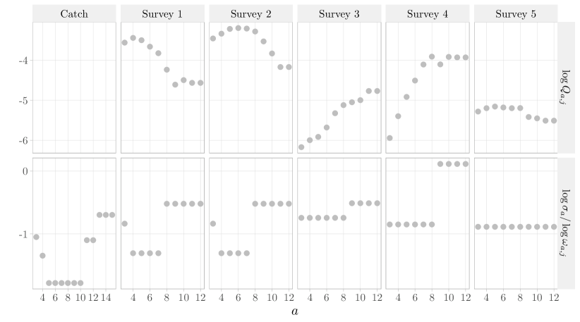
Figure 1: Age-dependent parameter estimates from the official SAM model for cod in the North-East Arctic. The upper rows for each fish stock contains estimates of $\log Q_{a,j}$ for all the different surveys. The lower rows contains estimates of $\log\sigma_{a}$ in the first column, and $\log\omega_{a,j}$ in the remaining columns.

We propose to improve the model-selection process by imposing a smooth structure on the age-dependent parameters. Thus, instead of estimating the parameters $(\theta_{1},\theta_{2},\ldots,\theta_{A})$, we estimate the parameters of a smooth parametric function $f_{\theta}(a)$ such that $\theta_{a}=f_{\theta}(a)$ for all $a=1,2,\ldots,A$. This can speed up the model selection process, since a modeller only needs to consider a few different smooth functions, instead of all $2^{A-1}$ possible partitions for each age-dependent parameter. It can also make the model selection process less subjective, while making the subjectivity of the modeller less tangible. When a modeller has chosen a partition of $\theta_{a}$, it might be difficult to understand why that specific partition was chosen. However, when a modeller chooses a smooth function $f_{\theta}$, all their assumptions are incorporated into that function. A model critic can then look at the function $f_{\theta}$, find that it e.g. allows for too abrupt changes, and modify it so it better suits their own assumptions.

We model the parameters $Q_{a,j}$, $\omega^{2}_{a,j}$ and $\sigma^{2}_{a}$ using smoothing splines. Smoothing of $F_{a,y}$ is outside the scope of this paper. This is because the fishing mortality rates are assumed to be correlated across years, which complicates any smoothing procedures. A spline function, $f(a)$, is a linear combination of polynomials,

$$f(a)=\sum_{i=1}^{n}\beta_{i}\phi_{i}(a),$$ (4)

where the $n$ parameters $\bm{\beta}=(\beta_{1},\ldots,\beta_{n})^{\top}$ describe the weights of each of the $n$ polynomials $\phi_{1},\ldots,\phi_{n}$, also known as the basis functions. Using matrix notation, the spline function can be written as $f(a)=\bm{x}^{\top}(a)\bm{\beta}$, where the vector $\bm{x}(a)$ contains all $n$ basis splines, evaluated at $a$. Furthermore, the vector $\bm{f}=(f(1),f(2),\ldots,f(A))^{\top}$ can be written as $\bm{f}=\bm{X}\bm{\beta}$, where the matrix $\bm{X}=(\bm{x}(1),\bm{x}(2),\ldots,\bm{x}(A))^{\top}$ contains all basis splines evaluated at all age groups.

Splines containing a large number of basis functions tend to be highly flexible and can easily overfit to the training data. It is therefore common to regularise the splines in some way by adding penalty terms to the likelihood function [16, e.g.]. These penalty terms can then be designed to penalise abrupt changes, too much wiggliness, too large absolute values, and many other properties of interest. We assume that the differences between age group 1 and 2 should be more considerable than the differences between e.g. age group 9 and 10. Therefore, we implement the smoothing splines as functions of $\log(a+1)$ instead of functions of $a$. In this log-space, the distance between age group 1 and 2 is as large as the distance between age group 3 and 5 and between age group 5 and 8. To constrain the spline parameters $\bm{\beta}$, our penalised log-likelihood takes the relatively common form

$$\mathcal{L}_{\bm{\lambda}}(\bm{\theta},\bm{\beta})=\ell(\bm{\theta},\bm{\beta})-\frac{1}{2}\sum_{i=1}^{M}\lambda_{i}\bm{\beta}^{\top}\bm{S}_{i}\bm{\beta},$$ (5)

where $\ell$ is the original log-likelihood without any penalty terms, $\bm{\theta}$ is a vector of all remaining model parameters and $\bm{S}_{1},\ldots,\bm{S}_{M}$ is a set of $M$ penalty matrices, describing which properties of $\bm{\beta}$ we wish to penalise. Finally, $\bm{\lambda}=(\lambda_{1},\ldots\lambda_{M})$ is a vector of $M$ penalty parameters, describing how much weight that should be given to each of the penalty matrices. $M$ is typically equal to either $1$ or $2$, as a large number of penalty parameters leads to overly complicated models.

We use the mgcv package [18] in R for designing and computing the penalty matrices and the values of the basis functions at all age groups of interest. mgcv makes it easy to design a large variety of different spline functions with different types of penalties. Note, that our developed SAM model is not constrained to using mgcv. It is method agnostic, in the sense that it only requires the matrices $\bm{X}$ and $\bm{S}_{1},\ldots,\bm{S}_{M}$ as input. To avoid subjective and time-demanding decisions about the number of basis functions during the model selection process, we set the number of basis functions equal to the number of age groups. Without any penalisation this would heavily increase the number of model parameters, and likely lead to considerable overfitting. However, given reasonable spline penalties, the parameters will be constrained in a way that reduces the wiggliness, and thus the effective number of parameters, to a suitable level for any data set in question. In Section 4, we choose two specific spline functions from mgcv for comparing our model framework against a selection of official SAM models. More details about these two spline functions are given there.

The smoothing penalty parameters $\bm{\lambda}$ should be large enough to reduce overfitting, but not so large that the splines loose all their flexibility. Optimal values for $\bm{\lambda}$ cannot be estimated by maximising the penalised log-likelihood (5), as this would result in a penalty of zero. From a Bayesian perspective, the penalised likelihood has the same mode and overall shape as a posterior distribution for $\bm{\beta}$ where the (improper) prior distribution of $\bm{\beta}$ is Gaussian with zero mean and “inverse covariance matrix” $\sum_{i=1}^{M}\lambda_{i}\bm{S}_{i}$ [11, 15, 19, e.g.]. Inspired by e.g. [17] and [19], we use this Bayesian perspective to estimate the model parameters and smoothing penalty parameters by maximising the logarithm of the “posterior” probability density function,

$$\ell(\bm{\theta},\bm{\beta})+\log\pi_{\bm{\lambda}}(\bm{\beta}),$$ (6)

where $\pi_{\bm{\lambda}}(\bm{\beta})$ is the probability density function of the Gaussian prior for $\bm{\beta}$. More details about the parameter estimation is provided in Appendix A.

4 Case study

4.1 Method

We compare the developed smoothing spline SAM with official SAMs for a large collection of stock assessment data sets. The webpage stockassessment.org contains stock assessment data for a large variety of fish stocks, together with official SAMs, where partitions for the age-dependent parameters already have been chosen. We download stock data together with their corresponding official models for 17 different stocks. These are listed in Table 1. The 17 stock data sets were chosen to represent a wide spread of different areas and fish stocks, given the constraint that we only want to model stock data sets where the corresponding SAM model is described as the final version on stockassessment.org. For each stock data set, we compare the official SAMs against competing smoothing spline SAMs, by examining parameter estimates, population estimates and log-likelihoods. Model comparison is also performed using cross-validation and forward-validation studies.

Table 1: All fish stock data used for the model evaluation. The columns Years catch/survey contain all years with available catch/survey data, Ages contains the minimum and maximum ages in the data set and Data source contains the names used to identify the data sets at stockassessment.org.

Fish stock	Area	Years catch	Years survey	Ages	Data source
Cod	Baltic Sea	1985 - 2021	1996 - 2022	0 - 7	WBcod22Fsq
Herring	Baltic Sea	1977 - 2021	1999 - 2021	0 - 8	GoR_BP_v2.2.3qF_s
Plaice	Baltic Sea	1999 - 2022	1999 - 2022	1 - 7	ple.27.21-23_WGBFAS_2023_ALT_v1
Cod	Celtic Sea	1980 - 2022	2002 - 2022	0 - 7	Cod_7ek_2023
Haddock	Celtic Sea	1993 - 2022	2003 - 2022	0 - 8	HAD7bk_2023_final
Plaice	Celtic Sea	1989 - 2021	1989 - 2021	1 - 10	Ple.7fg.2022.main
Whiting	Celtic Sea	1999 - 2022	2000 - 2022	0 - 7	whg.7b-ce-k_WGCSE22_RevRec_2023
Haddock	Faroe Plateau	1957 - 2023	1994 - 2023	1 - 10	NWWG2023_faroehaddock
Ling	Faroe Plateau	1996 - 2022	1996 - 2022	3 - 12	lin.27.5b_wgdeep2023_final
Saithe	Faroe Plateau	1961 - 2023	1994 - 2023	3 - 15	fsaithe-NWWG-2023
Cod	North-East Arctic	1946 - 2022	1981 - 2023	3 - 15	NEA_cod_2023_final_run
Saithe	North-East Arctic	1960 - 2021	1994 - 2021	3 - 12	NEAsaithe_2022_v3
Haddock	North Sea	1972 - 2022	1983 - 2023	0 - 8	NShaddock_WGNSSK2023_Run1
Plaice	North Sea	1957 - 2020	1970 - 2020	1 - 10	plaice_final_10fix
Sole	North Sea	1984 - 2021	1987 - 2021	1 - 9	Sole20_24_2022vs21
Whiting	North Sea	1978 - 2022	1983 - 2023	0 - 6	NSwhiting_2023
Blue whiting	Widely distributed	1981 - 2023	2004 - 2023	1 - 10	BW-2023

We develop two competing smoothing spline models, using two different spline functions from mgcv. The first model, denoted Spline1, uses a shrinkage version of a cubic regression spline (denoted cs in mgcv). The second model, denoted Spline2, uses a B-spline basis (denoted bs in mgcv) of order 3. Both models penalise the second derivative of the spline functions. For an improved comparison basis, we also evaluate a fourth model, denoted the Maximal model. In this model, the age-dependent parameters are not constrained in any way. This results in a highly flexible, but less robust model, with a large amount of parameters. The four competing models are listed and described in Table 2. Note that, while all four models use different configurations for the parameters $Q_{a,j}$, $\omega_{a,j}^{2}$ and $\sigma_{a}^{2}$, all other parameter configurations are kept unchanged from that of the official model. We use the default initial values in SAM for all four models. These are $\log Q_{a,j}=-5$ and $\log\omega_{a,j}=\log\sigma_{a}=-0.35$. We use an initial value of $0$ for the logarithms of the smoothing penalty parameters.

Table 2: Names and descriptions of the four competing models.

Model	Description
Official	The official model, with manually selected partitions of the age-dependent parameters, retrieved from stockassessment.org.
Spline1	$Q_{a,j}$, $\omega_{a,j}^{2}$ and $\sigma_{a}^{2}$ are modelled with shrinkage versions of a cubic regression spline (cs) that penalises large absolute values of the second derivatives. $\omega_{a,j}^{2}$ and $\sigma_{a}^{2}$ are given one common penalty parameter, that is the same for all values of $a$ and $j$. $Q_{a,j}$ is given its own penalty parameter, that is the same for all values of $a$ and $j$. This results in a total of $2$ penalty parameters for the entire model.
Spline2	$Q_{a,j}$, $\omega_{a,j}^{2}$ and $\sigma_{a}^{2}$ are modelled with splines based on B-spline bases of order 3 (bs) that penalises large absolute values of the second derivatives. $\omega_{a,j}^{2}$ and $\sigma_{a}^{2}$ are given one common penalty parameter, that is the same for all values of $a$ and $j$. $Q_{a,j}$ is given its own penalty parameter, that is the same for all values of $a$ and $j$. This results in a total of $2$ penalty parameters for the entire model.
Maximal	$Q_{a,j}$, $\omega_{a,j}^{2}$ and $\sigma_{a}^{2}$ are given independent parameters for all age groups of interest.

We evaluate the models’ performances using cross-validation and forward-validation. This is achieved by removing one or more years of data, fitting the competing models to the remaining data, and then predicting properties of the removed data. The best way of evaluating model performance would be to compare predicted populations with the true populations. This is clearly not possible, since the true populations are unknown. Instead, we evaluate the models by predicting catch-at-age data and survey indices, and comparing these to the true values. Our hope is that the model that is best at predicting catch-at-age data and survey indices also is the model that is best at estimating the true populations. Within SAM, one can easily estimate unknown catch-at-age data and survey indices for some year $y$, by setting all the observations from that year equal to NA.

Forward-validation is performed by fitting a model to all data from all years less than some year $y$ for a given fish stock data set. Then, we predict catch-at-age and survey indices for year $y$ using the fitted model. This can be unstable if one sets $y$ low enough that only a few years of data are available. We therefore restrict the forward-validation so that $y$ must be in the last third of the available years for each fish stock data set. Several data sets contain survey indices that have only been reported for a few years. Different values of $y$ might therefore lead to data sets containing only one or two years of data from a specific survey type. This can make it hard to reliably estimate the survey parameters for that survey type. We therefore also filter out data from any type of survey with less than five years of data before $y$. Cross-validation is achieved by only removing data from a single year, and predicting catches and survey indices for that year. This is more stable, since less data is removed. We therefore perform cross-validation for all available years except the first, and we never remove all the data from an entire type of survey.

The cross/forward-validation predictions are evaluated by computing the root mean squared error (RMSE) between predicted and observed catch-at-age data and survey indices. Catch-at-age RMSE values are computed by summing over the squares of the differences between $\tilde{C}_{a,y}$ and $\hat{C}_{a,y}$ for all age groups $a$ and all leave-out years $y$, where $\tilde{C}_{a,y}$ is predicted catch-at-age data obtained using the described cross-validation or forward-validation procedures. Survey index RMSE is computed similarly, where we sum over the squares of the differences between $\tilde{I}^{(j)}_{a,y}$ and $\hat{I}^{(j)}_{a,y}$ for all age groups $a$, all years of interest $y$ and all available survey types, where $\tilde{I}^{(j)}_{a,y}$ is a predicted survey index obtained using the described cross-validation or forward-validation procedures. During the forward-validation, we also perform a conditional catch-at-age prediction, where we predict catch-at-age values for year $y+1$ given that we know the total biomass of all catches for that year. One can think of this as predicting next years catch-at-age values given that the fishing quota for next year has been set, which is a highly realistic scenario. Conditional prediction is performed using the forecast() function in SAM. Having predicted conditional catch-at-age values, we then compute RMSE values just as we did for the unconditional catch-at-age values.

4.2 Results

Table 3: Convergence statistics for the cross/forward-validation.

Model	Convergence
Official	$1009/1015$	$\approx$	$99.4\%$
Spline1	$970/1015$	$\approx$	$95.6\%$
Spline2	$996/1015$	$\approx$	$98.1\%$
Maximal	$855/1015$	$\approx$	$84.2\%$
All	$810/1015$	$\approx$	$79.8\%$

In total, we fit each of the four SAM models to $1015$ different data sets during the cross/forward-validation. As some of the models are less robust than the others, and as no tweaking of initial values is performed, it is expected that not all four models will be able to converge successfully at first try for all the $1015$ different data sets. Table 3 displays the total number of successful convergences for each of the four models. As expected, the maximal model is the least robust, as it contains the largest number of parameters. Furthermore, the official model is the most robust, as it has been designed specifically for each fish stock data set by a panel of experts. Interestingly, the convergence rate of the spline2 model is only slightly lower than that of the official model. This is a promising result, as the spline models do not contain any prior knowledge about the shapes of $Q_{a,j}$, $\omega_{a,j}^{2}$ and $\sigma_{a}^{2}$, except the assumptions that these should behave somewhat smoothly as a function of $a$. No tweaking of initial values has been performed either. However, note that the remaining parameter configurations of the spline models are the same as in the official model. The bottom row shows that all four models successfully converged for $810$ of the $1015$ data sets. We only compute and compare RMSE values for these $810$ data sets, to make the model comparison as fair as possible.

For easier comparisons between the official model and its three competing models, we standardise the RMSE values by dividing all RMSE values from the competing models on their corresponding RMSE values from the official model. A standardised RMSE greater than $1$ means that the official model outperformed the competing model, while a standardised RMSE less than $1$ means the opposite. Figure 2 displays box-plots for the standardised RMSE values between the official model and the other three competing models, for all of the 17 fish stock data sets. Conditional prediction was not performed for Haddock or Saithe from the Faroe Plateau, as these stock data sets contained missing observations for at least one age group in almost every year used for forward-validation, which makes it impossible to condition on the total biomass of last years catches. Figure 2 show that all three models achieve standardised RMSE values that are both greater than $1$ and less than $1$ for all the different evaluation criteria. However, the main trend seems to be that all three of the competing models slightly outcompete the official model for most of the fish stock data sets. The spline1 model seems to perform the best overall, with respect to RMSE, as it achieves a standardised RMSE below 1 for the majority of the fish stocks in each of the five sub-plots. However, the spline2 model and the maximal model also seem to outperform the official model in most of the five subplots.

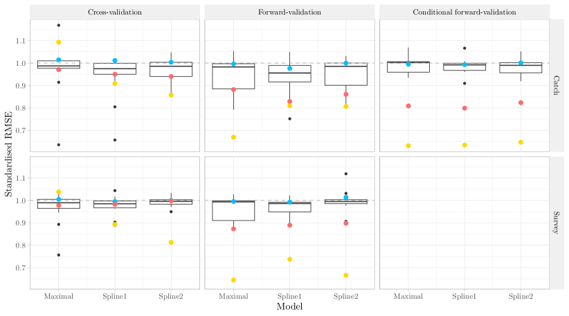
Figure 2: Box-plots displaying standardised RMSE values for the 17 different fish stock data sets in Table 1. The boxes span from the $25$ percentile to the $75$ percentile of the 17 standardised RMSE values, and the dark horisontal line within each box displays the standardised RMSE median. The leftmost column displays standardised RMSE values for catch-at-age data and survey indices from the cross-validation. The middle column displays the same for the forward-validation. The rightmost column displays standardised RMSE values for the conditional catch-at-age data from the forward-validation procedure. The blue, red and yellow dots correspond to the fish stocks in subplot A, B and C of Figure 3, respectively. The blue dot in the bottom left subplot is hidden behind the red dot.

We evaluate additional properties of the model fits by examining and comparing parameter estimates for each of the 17 fish stocks. Estimated values of $\log Q_{a,j}$, $\log\omega_{a,j}$ and $\log\sigma_{a}$ for three different fish stocks are given in Figure 3. Subplot A displays estimated parameters for cod in the North-East Arctic, in which the official model parameters are also displayed in Figure 1. All four competing models seem to agree well about the catchability ($Q_{a,j}$) estimates. The models also more-or-less agree about the variance estimates. The official model partition contains several subsets with 4-6 different parameters, while the other three models are less constrained, and therefore tend to vary more as a function of age. Still, the model differences are small, overall. The largest differences occur for $\omega_{a,2}$, where the three competing models produce smaller estimates. We are unsure why this happens. As shown by the blue dots in Figure 2, the cross/forward-validation also finds that all four models perform approximately equally well. However, the time and knowledge required to develop the official model is considerably larger than what is required for the other three models.

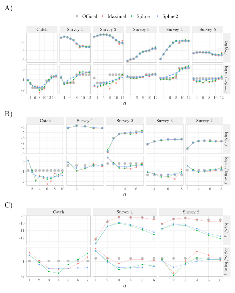
Figure 3: Age-dependent parameter estimates for three different fish stocks: A) Cod in the North-East Arctic, B) Plaice in the Celtic Sea and West of Scotland, C) Plaice in the Baltic Sea. The upper rows for each fish stock contains estimates of $\log Q_{a,j}$ for all the different surveys. The lower rows contains estimates of $\log\sigma_{a}$ in the first column, and $\log\omega_{a,j}$ in the remaining columns.

Subplot B of Figure 3 displays estimated parameters for plaice in the Celtic Sea and West of Scotland. All four models agree about the catchability estimates, while the differences are larger for the variance parameters. All the official variance parameters are age-independent, while the more flexible models claim that the variance should drop quickly for the first age groups, and then stay constant or slowly increase for the larger age groups. This added flexibility seems to lead to a considerable model improvement, because the official model is outperformed by the other three models in both the cross-validation and the forward-validation, as shown by the red dots in Figure 2.

Subplot C of Figure 3 displays estimated parameters for plaice in the Baltic Sea. This is the only one of the 17 fish stocks where we find considerable differences in the catchability estimates between different models. Since $\log\hat{I}_{a,y}^{(j)}(d)$ is a random variable with mean $\log\left(Q_{a,j}N_{a,y}(d)\right)$, a decrease in $Q_{a,j}$ must also lead to an increase in $N_{a,y}(d)$, or a large increase in $\omega_{a,j}$. As expected, $N_{a,y}(d)$ is therefore estimated to be considerably larger for the spline models than for the official and maximal models. Figure 4 displays the estimated stock spawning biomass (SSB) for each model. The spline models produce SSB values more than twice as large as for the two other models. Since the true SSB is unknown, it is impossible to say which model that is most correct. Still, it is concerning that such a small change to the parameter configuration can lead to so considerable changes in the estimated fish populations and SSB values. The changes in $Q_{a,j}$ seem to happen because the official model assumes identical catchability for the three oldest age groups, while the spline models believe that the catchability should decrease for the oldest age groups. If we modify the official model so the thee largest age groups can obtain different catchabilities, we find that it changes considerably and almost perfectly agrees with the spline2 model. It is unclear why the maximal model does not agree with the spline models. However, further examinations show that the maximal model fit is quite unstable, and small changes to its initial parameters can cause it to agree with the spline models. The yellow dots in Figure 2 show that the official model is considerably outperformed by the three competing models for most of the evaluation metrics, but that the maximal model performs worse during the cross-validation. This might be caused by the instability of the maximal model.

Figure 3 demonstrates the power of the splines models and the maximal model as diagnostic tools, not only as stand-alone SAM models. In subplot A, all models mostly agreed about the different parameter estimates, except from the estimates for $\omega_{a,2}$, which were considerably smaller for the maximal and the spline models. It is interesting to discover that different models can obtain different values for a single variance parameter, while all other variance parameters are equal. A modeller presented with this information might therefore spend more time on examining the parameter $\omega_{a,2}$ specifically, by focusing on its potential dependencies with other parameters in the SAM-model, and how different configurations or smoothness assumptions for $\omega_{a,2}$ can affect the overall model fit and performance. Similarly, in subplot B, the maximal model and the spline models all estimate that the variance parameters should be large for the youngest age groups and then decrease and flatten out as the age increases. Knowing this, a modeller might focus more on testing parameter configurations where the youngest age groups are given different variance parameters than the oldest age groups. In subplot C, we find the same variance parameter patterns as in subplot B. In addition, we find that small changes in parameter configurations can yield completely different population estimates. Clearly, this should be of interest to the modellers that created the official model. It might be that further investigations show that the official population estimates are the best ones, but one should probably investigate further why these large differences appear, and if that has any consequences for how the official model should be treated and/or further developed.

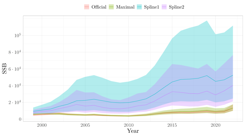
Figure 4: SSB for plaice in the Baltic Sea. The solid lines display the yearly estimated SSB values for each SAM model, while the shaded areas display estimated $95\%$ confidence intervals for the yearly SSB values.

5 Discussion

We propose modelling age-dependent parameters of the SAM model with smoothing splines as a guide to model development in stock assessment. This can lead to more realistic looking parameter estimates, as it reduces the discrete behaviour of the standard parameter partitioning method. Our method also makes it possible to automate and speed up model selection, and it allows for a less subjective model selection process. Finally, the spline method can be utilised as a diagnostics tool for suggesting initial values and starting points for partitioning the age-dependent parameters in the standard SAM model, and for examining the robustness of a model fit by comparing it to the fits of slightly different models.

We develop two different spline models, and compare them with the official SAM models for 17 different fish stock data sets. Cross-validation and forward-validation studies demonstrate that our spline models often outperform the official SAM models, while simultaneously requiring considerably less effort to be developed. Code for the two developed spline models are freely available online at https://github.com/NorskRegnesentral/SAM-spline, and can easily be used for modelling other fish stocks. Since the spline1 model demonstrated the highest performance, while the spline2 model was the most robust spline model, our recommendation for modellers interested in using these models would be to start by fitting the spline1 model to your data, and to switch to the spline2 model if they encounter convergence issues. However, our chosen spline functions are relatively standard in the literature, and not specifically tailored for stock assessment modelling. It might therefore be possible to develop more specialised spline functions that both perform better and that are more robust than our two spline models. Therefore, the available code online has been developed to make it easy to incorporate new types of smoothing splines into the SAM model, for modellers who are interested in experimenting with other model designs.

We also compare the official model with a maximal model, where all age groups are given separate parameters. The maximal model is also found to slightly outperform the official model, with regard to out-of-sample root mean squared error (RMSE) values. However, the model is less robust than its three competing models, in the sense that it more often fails to converge. It also has a tendency to more often produce considerably different parameter estimates when new years of data are added. Additionally, for 5 of the 17 fish stock data sets, the maximal model produces unrealistic parameter estimates, where the variance parameter for one specific age group suddenly becomes several orders of magnitudes smaller than the variance parameters of all other age groups and all other SAM models, while the neighbouring age groups are given variance parameters that are comparable to the other SAM models (results not shown). Still, we did not attempt to tweak the models that failed to converge, or to restart parameter estimation using different initial values. In a setting where multiple modellers focus on achieving convergence with the maximal model for one specific fish stock data set, it might be that convergence can be achieved easily with just a few minor changes to the model formulation or initial values. However, as the four models in Section 4 only are compared for data subsets where all four models converged, there are more than 200 data sets that were not used for model evaluation, where the official model converged, but the maximal did not. Since the maximal model seems to struggle for these data sets, it might be that any tweaking of initial values to improve the convergence rate would actually decrease model performance relative to the official model, as the two models would then have to be compared using data that are more unfavorable towards the maximal model. All in all, it is clear that the maximal model is less robust than the other three SAM models. However, given its promising performance for several of the fish stock data sets, the maximal model might still serve as a viable alternative for many different fish stock data sets, both as a competitive SAM model and as a diagnostics tool.

We would highlight that the model output (and hence quota advice) is sensitive to the parameter partitioning choices, i.e. which age-dependent parameters that are set equal to each other. The mis-specification identified is not a purely theoretical issue, but can undermine the model performance. The variance estimates are used within the model to allocate weight to different data sources during model fitting. Mis-specification of the partitioning structure can therefore have serious implications for the stock assessment, with the model either overly tuned to noisy data or erroneously downweighting reliable data. Producing a realistic parameter partitioning is therefore important to ensuring that there is a robust scientific underpinning to fisheries management.

Our developed smoothing spline extension of SAM is highly general, as it works for all types of parametric functions that can be written as a linear combination of parameters and basis functions, and it allows all penalisation structures that can be written as a quadratic polynomial of the parameters of interest. Thus, one can easily use our framework to model the age-dependent parameters using e.g. other types of spline models, 2. or 3. degree polynomials of age, trigonometric, logarithmic or exponential functions of age, or a combination of these. We chose to model the age-dependent parameters using cubic regression splines and B-splines of order 3, because these are relatively common spline models that are easy to implement using the mgcv package in R. However, given the considerable success of our these two relatively standard spline models, we believe that further work on designing spline functions and penalties can lead to further improvements to both model performance and model robustness.

A different approach for more flexible modelling of the variance parameters in SAM was proposed by [5]. They argue that the relationships between the variances and means of $\hat{C}_{a,y}$ and $\hat{I}^{(j)}_{a,y}$, which they denote the prediction-variance link, might be too constraining in the original SAM model, and they add some additional model parameters to make these relationships more flexible. In their examples, the modified prediction-variance links seem to remove much of the age-signals in $\sigma^{2}_{a}$ and $\omega^{2}_{a,j}$. This modified prediction-variance link might therefore reduce the need for spline modelling of $\sigma^{2}_{a}$ and $\omega^{2}_{a,j}$. We have not attempted to model the fish stocks from Section 4 using spline models and a modified prediction-variance link, but this might be an interesting topic for future research.

In this paper, we have only implemented and tested smoothing spline models for the parameters $Q_{a,j}$, $\omega_{a,j}^{2}$ and $\sigma^{2}_{a}$. However, many SAM models contain additional age-dependent parameters, and all contain the age- and year-dependent unknowns for the fishing pressure by age over time ($F_{a,y}$). These parameters have a direct impact on the model in terms of the dynamics of the modelled stock (which fish are killed each year) and through model tuning to data (which fraction of the caught fish are of a given age). Correct specification here is therefore extremely important for good model performance. Further work should therefore focus on implementing the smoothing splines for any additional parameters where this makes sense. $F_{a,y}$ might require some additional work, as it typically is assumed to vary over time, with a degree of autocorrelation. Furthermore, since spline modelling of other parameters than $Q_{a,j}$, $\omega_{a,j}^{2}$ and $\sigma^{2}_{a}$ where outside the scope of this paper, our spline models and maximal model relied on using parameter configurations from the official model for all other age-dependent parameters. Thus, it is not yet entirely correct that our developed models allow for a fully automated model selection procedure. However, the model selection procedure is fully automated for $Q_{a,j}$, $\omega_{a,j}^{2}$ and $\sigma^{2}_{a}$, and it has the potential of becoming fully automated if similar spline models can be implemented for all other age-dependent parameters.

As discussed, more work might be necessary for achieving robust and fully automated model selection for all age-dependent parameters. However, when it comes to using the spline as a diagnostics tool for the standard SAM model, no additional work is needed. Our method is easy to use, and readily available for anyone who are interested in stock assessment modelling. We believe that our method can be of great help for designing SAM models and for understanding the properties of an already developed SAM model even better. In particular the method outlined here can be used to validate the existing model structure, and serve as a guideline any revisions. We would therefore recommend that it be applied whenever a model revision is being conducted.

Code and data availability

The code used for extending the SAM model and for creating all results and figures in this paper is freely available online at https://github.com/NorskRegnesentral/SAM-spline. The data used in this paper is freely available online at stockassessment.org.

Conflict of interest

The authors declare no conflict of interest.

Funding

This work was funded by the Institute of Marine Research, Norway, through the 338 project “Rammeavtale for statistikk og beregningsmatematikk – Saksnr 20/03100”.

Appendix A Estimating the smoothing penalty parameter

[17] and [19] rely on a Bayesian perspective, described in Section 2, for estimating model parameters and smoothing penalty parameters by maximising the logarithm of the “posterior” distribution in (6), where $\pi_{\bm{\lambda}}(\bm{\beta})$ is the probability density function of the improper Gaussian prior for $\bm{\beta}$,

$$\pi_{\bm{\lambda}}(\bm{\beta})\propto\left\lvert\sum_{i=1}^{M}\lambda_{i}\bm{S}_{i}\right\rvert^{1/2}_{+}\exp\left(-\frac{1}{2}\bm{\beta}^{\top}\left(\sum_{i=1}^{M}\lambda_{i}\bm{S}_{i}\right)\bm{\beta}\right),$$ (A.1)

where $\lvert\bm{S}\rvert_{+}$ is the product of all non-zero eigenvalues of $\bm{S}$. Instead of estimating the spline parameters $\bm{\beta}$ and the penalty parameters $\bm{\lambda}$ simultaneously, they integrate the spline parameters out of the posterior distribution using a Laplace approximation to the marginal log-likelihood

$$\mathcal{V}(\bm{\theta},\bm{\lambda})=\log\int\exp(\ell(\bm{\theta},\bm{\beta}))\pi_{\bm{\lambda}}(\bm{\beta})\text{d}\bm{\beta}.$$ (A.2)

The SAM model is essentially implemented as a wrapper around the TMB package [12] in R, which contain built-in functionality for approximating marginal log-likelihood functions using the Laplace approximation. This makes it straightforward to approximate (A.2) using Laplace approximations. Note that the SAM implementation already relies on such Laplace approximations for integrating out $N_{a,y}$, $F_{a,y}$ and several other unknowns from its likelihood. See the openly available code of [4] for an example of how to estimate smoothing penalty parameters in a simplified stock assessment model, using a Laplace approximation to the marginal log-likelihood in (A.2).

Unfortunately, the Laplace approximation does not work well for random effects that are far from Gaussian distributed [12, e.g. ]. It appears that this might be the case for some of our random effects, because, when fitting our modified SAM model to fish stock data from Section 4, it often fails to converge, when using the Laplace approximation on the spline parameters in $\sigma_{a}^{2}$ and $\omega^{2}_{a,j}$. For this reason, we choose to not integrate out the variance spline parameters with the Laplace approximation. Instead, we estimate the penalty and spline parameters for the variance components simultaneously, using the default optimisation method within SAM. As mentioned in Section 2, simultaneous estimation of penalty and spline parameters is not possible when optimising over the log-likelihood function. However, the normalisation constant of the added prior distribution in (6) rewards larger penalty parameters, and thus makes it possible to estimate both $\bm{\beta}$ and $\bm{\lambda}$ simultaneously without the estimator for $\bm{\lambda}$ becoming equal to zero. Note that we still rely on the Laplace approximation for integrating out all spline parameters related to $Q_{a,j}$.

In practice, after testing our model on different stock assessment data sets, we find that further changes should be made to the SAM model to achieve more robust parameter estimation. The differences between the parameters for the smallest age groups are typically expected to be much larger than the differences for larger age groups. As described in Section 2, we therefore implement our splines as functions of $\log(a+1)$ instead of $a$. However, in our experience, this transformation is often not enough to fully account for the differences between large and small age groups. The need for varying degrees of wiggliness for small and large age groups can be problematic when estimating a single smoothing penalty parameter for all the age groups. Thus, we often find that a penalty parameter that is independent of age becomes too strict for small age groups and too lenient for large age groups. To account for this, we modify the smoothing penalty by down-weighting it for the youngest age groups. This is achieved by modifying the penalty matrices $\bm{S}_{i}$ into the matrices

$$\tilde{\bm{S}}_{i}=\bm{D}\bm{S}_{i}\bm{D}.$$ (A.3)

Here, the matrix $\bm{D}$ is a diagonal matrix with elements that are less than $1$ for the basis splines that are centred around the smallest age groups, and $1$ for all other basis splines. We set the diagonal elements for the basis splines corresponding to the three youngest age groups equal to $\exp(a-4)$, where $a\in\{1,2,3\}$.

For some stock assessment data sets, we experience weak age signals in $\sigma^{2}_{a,I}$. Sometimes, the age signals are so weak that the estimated splines prefer to be straight lines. This causes the penalty parameters to diverge towards infinity, which causes numerical problems. To obtain more numerically robust parameter estimates, we therefore extend the model in (A.2) by adding an improper prior distribution to $\bm{\rho}=\log\bm{\lambda}$ that penalises too large values of $\bm{\rho}$. Our chosen prior is essentially a uniform prior between negative infinity and some large constant $K$, with a small probability of allowing larger values than $K$, in case this becomes necessary. The probability density function of the improper prior is

$$\pi(\bm{\rho};K,\delta)=\prod_{i=1}^{M}\pi(\rho_{i};K,\delta)=\prod_{i=1}^{M}\frac{\exp(\delta(K-\rho_{i}))}{\left(1+\exp(\delta(K-\rho_{i}))\right)},$$ (A.4)

where we choose $K=7$ and $\delta=100$. The parameter $\delta$ describes how quickly the prior density should change from $1$ to $0$ as $\rho$ increases and grows larger than $K$. Figure A.1 displays the form of $\pi(\rho;K,\delta)$ for a set of different $\delta$-values, to visualise its effect on the prior. We choose this penalty prior for multiple reasons. This improper prior is approximately equal to one for all penalty parameters below $\exp(K)$, meaning that it does not affect our parameter estimation unless the penalty parameters become really large. Furthermore, the prior is smooth, continuous and gives positive probabilities to all values of $\bm{\rho}\in\mathbb{R}^{M}$, which is necessary for the automatic differentiation within TMB to work as it should.

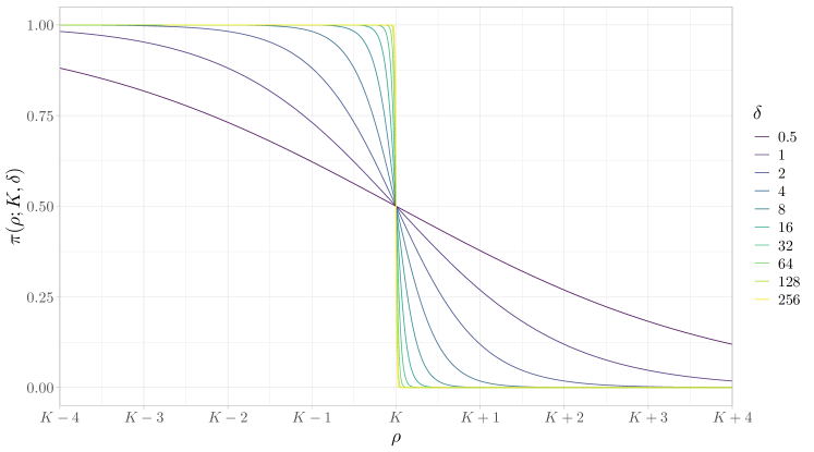
Figure A.1: Probability density function of the penalty prior, for a set of different values of $\delta$.

To summarise, after having included all of our changes, the final loss function that we use for estimating all model parameters, is

$$\ell(\bm{\theta},\bm{\beta})+\log\pi_{\bm{\lambda}}(\bm{\beta})+\log\pi(\bm{\lambda}),$$ (A.5)

where $\ell(\bm{\theta},\bm{\beta})$ is the log-likelihood of the original SAM-model, modified to let $Q_{a,j}$, $\omega_{a,j}^{2}$ and $\sigma_{a}^{2}$ be modelled using spline-functions. Furthermore, the $\bm{\beta}$-prior is an improper Gaussian prior with probability density function

$$\pi_{\bm{\lambda}}(\bm{\beta})\propto\left\lvert\sum_{i=1}^{M}\lambda_{i}\bm{D}\bm{S}_{i}\bm{D}\right\rvert^{1/2}_{+}\exp\left(-\frac{1}{2}\bm{\beta}^{\top}\left(\sum_{i=1}^{M}\lambda_{i}\bm{D}\bm{S}_{i}\bm{D}\right)\bm{\beta}\right),$$ (A.6)

and the improper $\bm{\lambda}$-prior has the probability density function given in (A.4), with $K=7$ and $\delta=100$. Then, using TMB, the spline parameters for $Q_{a,j}$ are integrated out with the Laplace approximation, along with several other model parameters that SAM integrates out by default.

References

- [1] M. Aldrin et al. “Caveats with estimating natural mortality rates in stock assessment models using age aggregated catch data and abundance indices” In Fisheries Research 243 Elsevier BV, 2021, pp. 106071 DOI: 10.1016/j.fishres.2021.106071
- [2] M. Aldrin, I.F. Tvete, S. Aanes and S. Subbey “The specification of the data model part in the SAM model matters” In Fisheries Research 229 Elsevier BV, 2020, pp. 105585 DOI: 10.1016/j.fishres.2020.105585
- [3] Casper W. Berg and Anders Nielsen “Accounting for correlated observations in an age-based state-space stock assessment model” In ICES Journal of Marine Science 73.7 Oxford University Press (OUP), 2016, pp. 1788–1797 DOI: 10.1093/icesjms/fsw046
- [4] Olav Nikolai Breivik et al. “Predicting abundance indices in areas without coverage with a latent spatio-temporal Gaussian model” In ICES Journal of Marine Science 78.6 Oxford University Press (OUP), 2021, pp. 2031–2042 DOI: 10.1093/icesjms/fsab073
- [5] Olav Nikolai Breivik, Anders Nielsen and Casper W Berg “Prediction-variance relation in a state-space fish stock assessment model” In ICES Journal of Marine Science 78.10 Oxford University Press (OUP), 2021, pp. 3650–3657 DOI: 10.1093/icesjms/fsab205
- [6] FAO “The State of World Fisheries and Aquaculture 2024” In The State of World Fisheries and Aquaculture (SOFIA), 2024 DOI: 10.4060/cd0683en
- [7] David Fournier and Chris P. Archibald “A General Theory for Analyzing Catch at Age Data” In Canadian Journal of Fisheries and Aquatic Sciences 39.8 Canadian Science Publishing, 1982, pp. 1195–1207 DOI: 10.1139/f82-157
- [8] Ray Hilborn et al. “Effective fisheries management instrumental in improving fish stock status” In Proceedings of the National Academy of Sciences 117.4 Proceedings of the National Academy of Sciences, 2020, pp. 2218–2224 DOI: 10.1073/pnas.1909726116
- [9] David Hirst et al. “A Bayesian modelling framework for the estimation of catch-at-age of commercially harvested fish species” In Canadian Journal of Fisheries and Aquatic Sciences 69.12 Canadian Science Publishing, 2012, pp. 2064–2076 DOI: 10.1139/cjfas-2012-0075
- [10] ICES “ICES Stock Information Database” https://sid.ices.dk [Accessed: 03.02.2025], 2025
- [11] George S. Kimeldorf and Grace Wahba “A Correspondence Between Bayesian Estimation on Stochastic Processes and Smoothing by Splines” In The Annals of Mathematical Statistics 41.2 Institute of Mathematical Statistics, 1970, pp. 495–502 DOI: 10.1214/aoms/1177697089
- [12] Kasper Kristensen et al. “TMB: Automatic Differentiation and Laplace Approximation” In Journal of Statistical Software 70.5 Foundation for Open Access Statistic, 2016 DOI: 10.18637/jss.v070.i05
- [13] Anders Nielsen and Casper W. Berg “Estimation of time-varying selectivity in stock assessments using state-space models” In Fisheries Research 158 Elsevier BV, 2014, pp. 96–101 DOI: 10.1016/j.fishres.2014.01.014
- [14] André E. Punt “Those who fail to learn from history are condemned to repeat it: A perspective on current stock assessment good practices and the consequences of not following them” In Fisheries Research 261 Elsevier BV, 2023, pp. 106642 DOI: 10.1016/j.fishres.2023.106642
- [15] Grace Wahba “Improper Priors, Spline Smoothing and the Problem of Guarding Against Model Errors in Regression” In Journal of the Royal Statistical Society Series B: Statistical Methodology 40.3 Oxford University Press (OUP), 1978, pp. 364–372 DOI: 10.1111/j.2517-6161.1978.tb01050.x
- [16] Simon N Wood “Stable and Efficient Multiple Smoothing Parameter Estimation for Generalized Additive Models” In Journal of the American Statistical Association 99.467 Informa UK Limited, 2004, pp. 673–686 DOI: 10.1198/016214504000000980
- [17] Simon N. Wood “Fast Stable Restricted Maximum Likelihood and Marginal Likelihood Estimation of Semiparametric Generalized Linear Models” In Journal of the Royal Statistical Society Series B: Statistical Methodology 73.1 Oxford University Press (OUP), 2010, pp. 3–36 DOI: 10.1111/j.1467-9868.2010.00749.x
- [18] Simon N. Wood “Generalized Additive Models: An Introduction with R” ChapmanHall/CRC, 2017 DOI: 10.1201/9781315370279
- [19] Simon N. Wood, Natalya Pya and Benjamin Säfken “Smoothing Parameter and Model Selection for General Smooth Models” In Journal of the American Statistical Association 111.516 Informa UK Limited, 2016, pp. 1548–1563 DOI: 10.1080/01621459.2016.1180986