Dimension-independent convergence rate of propagation of chaos and numerical analysis for McKean-Vlasov stochastic differential equations with coefficients nonlinearly dependent on measure

Abstract

In contrast to ordinary stochastic differential equations (SDEs), the numerical simulation of McKean-Vlasov stochastic differential equations (MV-SDEs) requires approximating the distribution law first. Based on the theory of propagation of chaos, particle approximation method is widely used. Then, a natural question is to investigate the convergence rate of the method (also referred to as the convergence rate of PoC). In fact, the PoC convergence rate is well understood for MV-SDEs with coefficients linearly dependent on the measure, but the rate deteriorates with dimension $d$ under the $L^{p}$-Wasserstein metric for nonlinear measure-dependent coefficients, even when Lipschitz continuity with respect to the measure is assumed. The main objective of this paper is to establish a dimension-independent convergence result of PoC for MV-SDEs whose coefficients are nonlinear with respect to the measure component but Lipschitz continuous. As a complement we further give the time discretization of the equations and thus verify the convergence rate of PoC using numerical experiments.

Keywords:  McKean-Vlasov stochastic differential equations (MV-SDEs); Propagation of chaos (PoC); Tamed Euler-Maruyama(EM) method; Convergence rate; Dimension-independent.

1 Introduction

This paper establishes the convergence rate of propagation of chaos (PoC) under the $L^{p}$-Wasserstein metric and the $L^{p}$ convergence rate of the tamed Euler-Maruyama(EM) method to the McKean-Vlasov stochastic differential equations (MV-SDEs) with super-linear growth in the spatial component in the drift and Lipschitz continuity in the measure component. MV-SDEs refer to the whole family of SDEs whose coefficients depend not only on the state components but also on their probability distributions. These equations were first proposed by H. McKean as a stochastic model naturally associated with a class of nonlinear parabolic equations ([31, 32]), and are now widely studied due to their important applications in areas such as statistical physics (see e.g. [30, 24]), mathematical biology ([3, 8]), mathematical finance([43]), among others.

MV-SDEs, being clearly more involved than the classical Itô’s SDEs, let us first introduce some studies on the well-posedness of the exact solution of such equations. Strong existence and uniqueness results under global Lipschitz conditions were established via fixed-point theorems ([38, 9, 2]). Subsequent work extended these results to cases with one-sided Lipschitz drift and globally Lipschitz diffusion coefficients ([15] and [40]). [25] proved existence and uniqueness for MV-SDEs with superlinear growth in both drift and diffusion coefficients. Further studies on well-posedness can be found in [5, 11, 34, 41, 12] and related references.

Despite theoretical guarantees on well-posedness, explicit solutions for MV-SDEs with superlinear coefficients remain elusive, necessitating numerical methods. The numerical framework McKean-Vlasov equations were initially proposed in [7] and have been investigated further in a number of more recent works. Ref. [7] suggests that the numerical discretization of MV-SDEs should involve two steps: first, approximating the true measures in the coefficients with empirical measures; second, time discretization of the resulting particle system. To be more specific, consider the MV-SDEs of the form

$${\rm d}x_{t}=f(x_{t},\mu_{t}^{x}){\rm d}t+g(x_{t},\mu_{t}^{x}){\rm d}W_{t},~t\in[0,T],$$ (1)

where $\mu_{t}^{x}$ denotes the law of the process $x$ at time $t$, i.e., $\mu_{t}^{x}=\mathbb{P}\circ x_{t}^{-1}$. To simulate this system, we expand it by introducing $N$ independent copies of $(x_{0},W)$, each generating a particle through

$${\rm d}x_{t}^{i}=f(x_{t}^{i},\mu_{t}^{x^{i}}){\rm d}t+g(x_{t}^{i},\mu_{t}^{x^{i}}){\rm d}W^{i}_{t}.$$ (2)

Let these particles interact with each other through their empirical measure, i.e., introduce $X_{t}^{i,N}$, the solution of the following interacting particle system

$${\rm d}X_{t}^{i,N}=f(X_{t}^{i,N},\mu_{t}^{X,N}){\rm d}t+g(X_{t}^{i,N},\mu_{t}^{X,N}){\rm d}W^{i}_{t},\quad X_{0}^{i,N}=x_{0}^{i},$$ (3)

where $\mu_{t}^{X,N}=\frac{1}{N}\sum_{j=1}^{N}\delta_{X_{t}^{j,N}}$ is the empirical measure. As shown in [7], the empirical distribution $\mu_{t}^{X,N}$ converges to $\mu_{t}^{x^{i}}$ (and by uniqueness $\mu_{t}^{x^{i}}=\mu_{t}^{x}$), enabling approximation of the true measure. With this particle approximation in hand, discretizing (3) in time yields a numerical solution for the MV-SDEs (1).

Along this line, analyzing the convergence of numerical solutions to (1) requires studying the PoC rate, i.e., the convergence of the interacting particle system (3) to the non-interacting limit(2). While Wasserstein convergence rates for linear functionals of measures are well understood, nonlinear functionals often exhibit dimension-dependent rates under Wasserstein metrics ([10, 16, 18, 17, 39]). However, some recent work suggest that a dimension-independent $\mathcal{O}(N^{-1/2})$ rate is achievable for specific classes of MV-SDEs ([13, 33, 39]). Moreover, the dimension-independent $\mathcal{O}(N^{-1/2})$ rate is estimated numerically in [12], and the authors highlight gaps in theoretical results, underscoring the need for further study. In this paper, we propose a specific class of MV-SDEs whose coefficients nonlinearly dependent on the measure, and prove a dimension-independent $\mathcal{O}(N^{-1/2})$ PoC rate under the $L^{p}(p\geq 2)$-Wasserstein metric. This is a different set of sufficient conditions compared to the existing results in the literature with the same rate, such as Lemma 5.1 in [13] and Theorem 4.2 in [39]. Furthermore, note that the computational cost of simulating a particle system is $\mathcal{O}(N^{2})$ at each time step, methods to reduce the cost can be found such as the projected particle method in [6] and the random batch method in [21, 22], but this issue is not considered in the present paper.

To demonstrate the eventual convergence of the numerical approximation and to give numerical tests, one needs to prove that the time-stepping scheme for the interacting particle system is convergent. Inspired by the numerical methods for SDEs([19, 23, 42, 37]), there are a few of results focus on the analysis of the time-stepping methods for MV-SDEs with various continuity coefficients. For example, for MV-SDEs with one-sided Lipschitz drift in the state variable, [14] analyzed strong convergence for the tamed EM method and the drift-implicit EM method, [35] proposed an adaptive EM scheme, [4] introduced a tamed Milstein scheme. While under a general Khasminskii-type condition, instead of imposing a one-sided and global Lipschitz condition on the drift and diffusion coefficients, respectively, [25] applied both tamed EM and Milstein schemes, [18] developed the truncated EM scheme. Here, we use the tamed EM method for time discretization and show that it converges with order $\mathcal{O}(\Delta^{1/2})$ which is consistent with the classical results.

This paper is organized as follows: Section 2 outlines notations and the preliminary analysis. Section 3 shows that the strong PoC rate could be $\mathcal{O}(N^{-1/2})$ and dimension-independent for the proposed nonlinear MV-SDEs, and establishes the $L^{p}$-convergence of the tamed EM method simutaneously. Section 4 presents numerical experiments to validate the theoretical PoC rate.

2 Preliminaries and notations

2.1 Notations

Throughout this paper, let $(\Omega,\mathcal{F},\left\{\mathcal{F}_{t}\right\}_{t\geq 0},\mathbb{P})$ be a complete probability space with a filtration $\left\{\mathcal{F}_{t}\right\}_{t\geq 0}$ satisfying the usual conditions (i.e., it is right continuous and $\mathcal{F}_{0}$ contains all $\mathbb{P}$-null sets), and let $\mathbb{E}$ denote the expectation corresponding to $\mathbb{P}$. Let $|x|$ denote the Euclidean vector norm and $\langle x,y\rangle$ denote the inner product of vectors $x,y$. If $A$ is a vector or matrix, its transpose is denoted by $A^{\rm T}$. If A is a matrix, let $|A|$ denote its trace norm, i.e., $|A|=\sqrt{{\rm trace}(A^{\rm T}A)}$. In addition, we use $\mathcal{P}(\mathbb{R}^{d})$ to denote the family of all probability measures on $(\mathbb{R}^{d},\mathcal{B}(\mathbb{R}^{d}))$, where $\mathcal{B}(\mathbb{R}^{d})$ denotes the Borel $\sigma$-field over $\mathbb{R}^{d}$, and define the subset of probability measures with finite $p$-th moment by

$$\mathcal{P}_{p}(\mathbb{R}^{d}):=\left\{\mu\in\mathcal{P}(\mathbb{R}^{d})\Big{|}\int_{\mathbb{R}^{d}}|x|^{p}\mu(dx)<\infty\right\}.$$

For $\mu,\sigma\in\mathcal{P}_{p}(\mathbb{R}^{d}),p\geq 1$, the Wasserstein distance between $\mu$ and $\sigma$ is defined as

$$\mathbb{W}_{p}(\mu,\sigma):=\inf_{\pi\in\mathcal{C}(\mu,\sigma)}\left(\int_{\mathbb{R}^{d}\times\mathbb{R}^{d}}|x-y|^{p}\pi(dx,dy)\right)^{1/p}$$

where $\mathcal{C}(\mu,\sigma)$ means all the couplings of $\mu$ and $\sigma$, i.e., $\pi\in\mathcal{C}(\mu,\sigma)$ if and only if $\pi(\cdot,\mathbb{R}^{d})=\mu(\cdot)$ and $\pi(\mathbb{R}^{d},\cdot)=\sigma(\cdot)$. For $t\in[0,T]$, $p>0$, $L_{t}^{p}(\mathbb{R}^{d})$ denotes the family of $\mathbb{R}^{d}$-valued $\mathcal{F}_{t}$-measurable random variables $\xi$ with $\mathbb{E}|\xi|^{p}<\infty$. As usual notations, “i.i.d.” means “independent and identically distributed”. In this paper we will often use the following fundamental inequality

$$\left(\sum_{i=1}^{n}|a_{i}|\right)^{r}\leq n^{r-1}\sum_{i=1}^{n}|a_{i}|^{r},r\geq 1.$$ (4)

Throughout this paper, $C$ denotes a generic positive constant that may change from line to line, and may depend on the initial data $x_{0}$ and the terminal time $T$ (and other fixed data), but is always independent of the dimension $d$ and the constants $\Delta$ and $N$ (associated with the numerical scheme and specified below).

2.2 Problem formulation

Let $x_{0}\in L_{0}^{p}(\mathbb{R}^{d})$ for some given $p\geq 2$ and independent of the $m$-dimensional Brownian motion $W$, $(x_{0}^{i},W^{i}),i=1,2,\dots,N$ are independent copies of $(x_{0},W)$. In the following, we work on the nonlinear MV-SDEs: for $i=1,2,\dots,N$,

$${\rm d}x_{t}^{i}= a(x_{t}^{i}){\rm d}t+f(x_{t}^{i},\mu_{t}^{x^{i}}){\rm d}t+g(x_{t}^{i},\mu_{t}^{x^{i}}){\rm d}W^{i}_{t},~t>0$$ (5)

with

$$f(x,\mu)=A\left(\int_{\mathbb{R}^{d}}\kappa(x,y)\mu({\rm d}y)\right),~g(x,\mu)=B\left(\int_{\mathbb{R}^{d}}\zeta(x,y)\mu({\rm d}y)\right)$$ (6)

where $\mu_{t}^{x}$ denotes the law of the process $x$ at time $t$, i.e., $\mu_{t}^{x}=\mathbb{P}\circ x_{t}^{-1}$, and the interacting particle system

$${\rm d}X_{t}^{i,N,\delta}= \tilde{a}(X_{\delta_{t}}^{i,N,\delta}){\rm d}t+f(X_{\delta_{t}}^{i,N,\delta},\mu_{\delta_{t}}^{X,N,\delta}){\rm d}t+g(X_{\delta_{t}}^{i,N,\delta},\mu_{\delta_{t}}^{X,N,\delta}){\rm d}W^{i}_{t},~t>0$$ (7)

where $\delta_{t}=[t/\delta]\delta$ for $\delta>0$, $[t/\delta]$ denotes the integer part of $t/\delta$. $\mu_{t}^{X,N,\delta}=\frac{1}{N}\sum_{j=1}^{N}\delta_{X_{t}^{j,N,\delta}}$, $a,\tilde{a}:\mathbb{R}^{d}\to\mathbb{R}^{d}$, $A:\mathbb{R}^{d}\to\mathbb{R}^{d}$, $\kappa:\mathbb{R}^{d}\times\mathbb{R}^{d}\to\mathbb{R}^{d}$, $B:\mathbb{R}^{d\times m}\to\mathbb{R}^{d\times m}$, $\zeta:\mathbb{R}^{d}\times\mathbb{R}^{d}\to\mathbb{R}^{d\times m}$.

The main aim in this section is to establish the following estimate:

$$\mathbb{E}|x_{t}^{i}-X_{t}^{i,N,\delta}|^{p}\leq C\left\{N^{-p/2}+(t-\delta_{t})^{p/2}+\mathbb{E}|a(X_{t}^{i,N,\delta})-\tilde{a}(X_{t}^{i,N,\delta})|^{p}\right\}.$$ (8)

for $t\in[0,T]$ with $T$ is the given terminal time. Next, let us explain why we focus on the systems (5) and (7), and consider the estimate (8). This is primarily based on the following facts:

• In (7), once we take $\tilde{a}=a,\delta=t$, then $\delta_{t}=t$ and (7) becomes

  $${\rm d}X_{t}^{i,N}= a(X_{t}^{i,N}){\rm d}t+f(X_{t}^{i,N},\mu_{t}^{X,N}){\rm d}t+g(X_{t}^{i,N},\mu_{t}^{X,N}){\rm d}W^{i}_{t},$$ (9)

  where we set $X_{t}^{i,N}:=X_{t}^{i,N,t},\mu_{t}^{X,N}:=\mu_{t}^{X,N,t}$ for the notational brevity. It is easy to see that (5) and (9) are the non-interacting particle system and the interacting particle system corresponding to the MV-SDEs

  $${\rm d}x_{t}= a(x_{t}){\rm d}t+f(x_{t},\mu_{t}^{x}){\rm d}t+g(x_{t},\mu_{t}^{x}){\rm d}W_{t},~t>0,$$

  respectively, and as an immediate by-product of (8), the PoC result

  $$\mathbb{W}_{p}(\mu_{t}^{x^{i}},\mu_{t}^{X^{i,N}})\leq\left(\mathbb{E}|x_{t}^{i}-X_{t}^{i,N}|^{p}\right)^{1/p}\leq CN^{-1/2}$$

  will be established.

• If the coefficients of equation (5) are all linearly growing, it is well known that the EM scheme is the simplest method to simulate the MV-SDEs: for a step size $\Delta>0$, $\underline{t}:=[t/\Delta]\Delta$,

  $${\rm d}X_{t}^{i,N,\Delta}= a(X_{\underline{t}}^{i,N,\Delta}){\rm d}t+f(X_{\underline{t}}^{i,N,\Delta},\mu_{\underline{t}}^{X,N,\Delta}){\rm d}t+g(X_{\underline{t}}^{i,N,\Delta},\mu_{\underline{t}}^{X,N,\Delta}){\rm d}W^{i}_{t}.$$

  Obviously, the scheme is included in (7) by taking $\tilde{a}=a$ and $\delta=\Delta$. However, this routine does not work for the MV-SDEs with non-globally Lipschitz continuous coefficients, and we must use the variants of the EM method. Inspired by [20, 28, 29], tamed EM and truncated EM methods have been well developed for MV-SDEs([14, 18, 25]). Suppose that $f$ and $g$ are Lipschitz continuous, and $a$ is one-sided Lipschitz continuous, if we set $\delta=\Delta$, take

  $$\tilde{a}(x)=\frac{a(x)}{1+\Delta^{\gamma}|a(x)|}$$

  for $\gamma\in(0,1/2]$, or

  $$\tilde{a}(x)=a\left(\Big{(}|x|\wedge\varphi^{-1}(h(\Delta))\Big{)}\frac{x}{|x|}\right),$$

  where the precise definitions of the functions $\varphi$ and $h$ can be found in [18], then (7) becomes the tamed EM and truncated EM schemes for system (5), respectively, and (8) gives the convergence result of the numerical scheme, as long as we further give the error estimate between $a$ and $\tilde{a}$.

Accordingly, we can simultaneously determine the convergence rate of both the propagation of chaos and the time discretization method, provided that (8) holds, rather than analyzing them separately.

2.3 Error estimate between (5) and (7)

Before starting our work, the first natural thing to do is to ensure that equations (5) and (7) have unique solutions, we do these under the following settings.

Assumption 2.1.

There is a constant $L>0$ such that

$$|a(0)|\vee|A(0)|\vee|\kappa(0,0)|\vee|B(0)|\vee|\zeta(0,0)|\leq L.$$

Assumption 2.2.

There are constants $\lambda_{1}\in\mathbb{R}$ and $L_{1},q>0$ such that

$$\langle x-y,a(x)-a(y)\rangle\leq \lambda_{1}|x-y|^{2},$$

$$|a(x)-a(y)|\leq L_{1}(1+|x|^{q}+|y|^{q})|x-y|$$

for all $x,y\in\mathbb{R}^{d}$.

Assumption 2.3.

There are constants $\lambda_{2},\lambda_{3},L_{2},L_{3}>0$ such that

$$|A(x)-A(y)|\leq \lambda_{2}|x-y|,\quad|\kappa(x,y)-\kappa(\bar{x},\bar{y})|\leq L_{2}(|x-\bar{x}|+|y-\bar{y}|),$$

$$|B(x)-B(y)|\leq \lambda_{3}|x-y|,\quad|\zeta(x,y)-\zeta(\bar{x},\bar{y})|\leq L_{3}(|x-\bar{x}|+|y-\bar{y}|)$$

for all $x,y,\bar{x},\bar{y}\in\mathbb{R}^{d}$.

Assumption 2.4.

Let $p\geq 2$, suppose that there exists a unique solution to (7) for any $i\in\{1,2,\dots,N\}$, and

$$\sup_{1\leq i\leq N}\left\{\mathbb{E}\left(\sup_{0\leq t\leq T}|X_{t}^{i,N,\delta}|^{p}\right)\vee\mathbb{E}\left(\sup_{0\leq t\leq T}|\tilde{a}(X_{t}^{i,N,\delta})|^{p}\right)\right\}\leq C.$$

Assumption 2.4 will be verified in the later when we take $\tilde{a}$ and $\delta$ as specific expressions.

Remark 2.1.

It is well known that Assumption 2.1 imply the following growth conditions of the coefficients:

$$\langle x,a(x)\rangle= \langle x-0,a(x)-a(0)\rangle+\langle x,a(0)\rangle\leq\lambda_{1}|x|^{2}+\frac{|x|^{2}}{2}+\frac{|a(0)|^{2}}{2}\leq(\lambda_{1}+\frac{1}{2})|x|^{2}+\frac{L^{2}}{2},$$

$$|a(x)|\leq |a(x)-a(0)|+|a(0)|\leq L_{1}(|x|+|x|^{q+1})+L,$$

and similarly,

$$|A(x)|\leq \lambda_{2}|x|+L,~|\kappa(x,y)|\leq L_{2}(|x|+|y|)+L,$$

$$|B(x)|\leq \lambda_{3}|x|+L,~|\zeta(x,y)|\leq L_{3}(|x|+|y|)+L$$

Remark 2.2.

According to Assumption 2.1, using the Kantorovich-Rubinstein dual representation of the Wasserstein distance $\mathbb{W}_{1}$:

$$\mathbb{W}_{1}(\mu,\sigma)=\sup\left\{\int_{\mathbb{R}^{d}}\phi(x)\mu({\rm d}x)-\int_{\mathbb{R}^{d}}\phi(x)\sigma({\rm d}x)\Bigg{|}\phi{\text{~}Lipschitz~continuous~with}~\sup_{x\neq y}\frac{|\phi(x)-\phi(y)|}{|x-y|}\leq 1\right\}$$

and the fact that $\mathbb{W}_{1}(\mu,\sigma)\leq\mathbb{W}_{2}(\mu,\sigma)$, it is easy to verify that the following inequalities subsequently hold

$$|f(x,\mu)-f(y,\sigma)|\leq C\big{(}|x-y|+\mathbb{W}_{2}(\mu,\sigma)\big{)},$$

$$|g(x,\mu)-g(y,\sigma)|\leq C\big{(}|x-y|+\mathbb{W}_{2}(\mu,\sigma)\big{)},$$

$$|f(0,\delta_{0})|+|g(0,\delta_{0})|\leq C$$

for all $x,y\in\mathbb{R}^{d}$ and all $\mu,\sigma\in\mathcal{P}_{2}(\mathbb{R}^{d})$, where $\delta_{0}$ denotes the delta distribution centered at the point 0.

Based on Remark 2.2, we can obtain the existence, uniqueness and boundedness of the solution of equation (5) following Theorem 3.3 in [15].

Lemma 2.1.

Let $p\geq 2$, for any $i=1,2,\dots,N$, under Assumption 2.1, there exists a unique solution $x_{t}^{i}$ to the equation (5), and the solution satisfies

$$\mathbb{E}\left(\sup_{0\leq t\leq T}|x_{t}^{i}|^{p}\right)\leq C.$$

Theorem 2.1.

Let $p\geq 2$, it holds under Assumptions 2.1-2.4 that

$$\mathbb{E}\left(\sup_{0\leq t\leq T}|x_{t}^{i}-X_{t}^{i,N,\delta}|^{p}\right)\leq CN^{-p/2}+C\sup_{0\leq t\leq T}(t-\delta_{t})^{p/2}+C\mathbb{E}\left(\sup_{0\leq t\leq T}|a(X_{t}^{i,N,\delta})-\tilde{a}(X_{t}^{i,N,\delta})|^{p}\right)$$

for all $i=1,2,\dots,N$.

The proof is postponed to the appendix.

3 Main results

3.1 Strong quantitative propagation of chaos

As we explained in the subsection 2.2, if we take $\tilde{a}=a$ and $\delta=t$ in (7), which implies $\delta_{t}=t$, let $X_{t}^{i,N}:=X_{t}^{i,N,t}$, then (7) becomes

$${\rm d}X_{t}^{i,N}= a(X_{t}^{i,N}){\rm d}t+A\left(\frac{1}{N}\sum_{j=1}^{N}\kappa(X_{t}^{i,N},X_{t}^{i,N})\right){\rm d}t+B\left(\frac{1}{N}\sum_{j=1}^{N}\zeta(X_{t}^{i,N},X_{t}^{i,N})\right){\rm d}W^{i}_{t},$$ (10)

which is the corresponding interacting particle system of (5)-(6), and the following quantitive convergence rate of PoC follows as an immediate by-product of Theorem 2.1

Theorem 3.1.

Let $p\geq 2$, it holds under Assumptions 2.1-2.3 that

$$\mathbb{E}\left(\sup_{0\leq t\leq T}|x_{t}^{i}-X_{t}^{i,N}|^{p}\right)\leq CN^{-p/2}.$$

According to the definition of $\mathbb{W}_{p}$-metric, we can get the following result directly.

Corollary 3.2.

For $p\geq 2$, under the conditions of Theorem 3.1,

$$\sup_{1\leq i\leq N}\mathbb{W}_{p}(\mu_{t}^{x^{i}},\mu_{t}^{X^{i,N}})\leq CN^{-1/2},$$

where $\mu_{t}^{X^{i,N}}$ denotes the marginal law of $X^{i,N}$ at the time $t$.

In fact, in the case where the coefficients of MV-SDEs are linear in measure, i.e.,

$$f(x,\mu)=\int_{\mathbb{R}^{d}}\kappa(x,y)\mu({\rm d}y),~g(x,\mu)=\int_{\mathbb{R}^{d}}\zeta(x,y)\mu({\rm d}y),$$

[38] showed that $\mathbb{W}_{2}(\mu_{t}^{x^{i}},\mu_{t}^{X^{i,N}})=\mathcal{O}(N^{-1/2})$. While in the case of Lipschitz continuous dependence in measure in the $\mathbb{W}_{2}$-metric, the rate of strong PoC deteriorates with the dimension $d$, for instance, the PoC rate under the $L^{2}$-norm presented in [14, 12, 10] is

$$\sup_{1\leq i\leq N}\mathbb{E}\left(\sup_{0\leq t\leq T}|x_{t}^{i}-X_{t}^{i,N}|^{2}\right)\leq C\begin{cases}N^{-1/2}&{\rm if}~~d<4,\\ N^{-1/2}\log(N)&{\rm if}~~d=4,\\ N^{-2/d}&{\rm if}~~d>4,\end{cases}$$

the rate under the $L^{p}$-norm for $p>0$ and $q>p$ given in [18, 27] is

$$\sup_{1\leq i\leq N}\sup_{0\leq t\leq T}\mathbb{E}|x_{t}^{i}-X_{t}^{i,N}|^{p}\leq C\begin{cases}N^{-1/2}+N^{-(q-p)/q}&{\rm if}~~p>d/2~~{\rm and}~~q\neq 2p,\\ N^{-1/2}\log(N)+N^{-(q-p)/q}&{\rm if}~~p=d/2~~{\rm and}~~q\neq 2p,\\ N^{-2/d}+N^{-(q-p)/q}&{\rm if}~~p\in[2,d/2)~~{\rm and}~~q\neq d/(d-p).\end{cases}$$ (11)

It can be observed that the PoC rate presented above depends on the dimension of the system and decays at approximately $O(N^{-1/2p})$ under the $\mathbb{W}_{p}$-distance when $p>d/2$. Note that, in this work, we treat a case of MV-SDEs with coefficients Lipschitz continuous dependence in measure, and prove a dimension-independent PoC rate of $\mathcal{O}(N^{-1/2})$ under the $\mathbb{W}_{p}$-distance. This paper significantly contributes to this area by extending previous findings.

3.2 Strong convergence rate of the tamed EM method

In the following, let $M\in\mathbb{Z}_{+}$, $\Delta=T/M$ be the step size, we take $\delta=\Delta$ and

$$\tilde{a}(x)=\frac{a(x)}{1+\sqrt{\Delta}|a(x)|},$$

in (7), and establish the convergence of the tamed EM method for the particle system (5). It is easy to known that

$$|\tilde{a}(x)|\leq\min\{|a(x)|,\Delta^{-1/2}\},$$ (12)

and $\delta_{t}=[t/\Delta]\Delta$, then (7) becomes

$${\rm d}X_{t}^{i,N,\Delta}= \frac{a(X_{\delta_{t}}^{i,N,\Delta})}{1+\sqrt{\Delta}|a(X_{\delta_{t}}^{i,N,\Delta})|}{\rm d}t+A\left(\frac{1}{N}\sum_{j=1}^{N}\kappa(X_{\delta_{t}}^{i,N,\Delta},X_{\delta_{t}}^{i,N,\Delta})\right){\rm d}t+B\left(\frac{1}{N}\sum_{j=1}^{N}\zeta(X_{\delta_{t}}^{i,N,\Delta},X_{\delta_{t}}^{i,N,\Delta})\right){\rm d}W^{i}_{t},$$ (13)

which is in accordance with the continuous version of the tamed EM method for (5).

Under the settings above, we can verify Assumption 2.4 easily.

Lemma 3.1.

Let $p\geq 2$, under Assumptions 2.1-2.3, it holds that

$$\sup_{1\leq i\leq N}\left\{\mathbb{E}\left(\sup_{0\leq t\leq T}|X_{t}^{i,N,\Delta}|^{p}\right)\vee\mathbb{E}\left(\sup_{0\leq t\leq T}|\tilde{a}(X_{t}^{i,N,\Delta})|^{p}\right)\right\}\leq C.$$

Proof.

For any $i\in\{1,\dots,N\}$, using the Itô formula to $|X_{t}^{i,N,\Delta}|^{p}$ with $X_{t}^{i,N,\Delta}$ satisfies (13), we have

$$|X_{t}^{i,N,\Delta}|^{p}\leq |x_{0}^{i}|^{p}+p\int_{0}^{t}|X_{s}^{i,N,\Delta}|^{p-2}\left\langle X_{s}^{i,N,\Delta},\tilde{a}(X_{\delta_{s}}^{i,N,\Delta})\right\rangle{\rm d}s$$

$$+p\int_{0}^{t}|X_{s}^{i,N,\Delta}|^{p-1}\left|A\left(\frac{1}{N}\sum_{j=1}^{N}\kappa(X_{\delta_{s}}^{i,N,\Delta},X_{\delta_{s}}^{j,N,\Delta})\right)\right|{\rm d}s$$

$$+p\int_{0}^{t}|X_{s}^{i,N,\Delta}|^{p-1}\left|B\left(\frac{1}{N}\sum_{j=1}^{N}\zeta(X_{\delta_{s}}^{i,N,\Delta},X_{\delta_{s}}^{j,N,\Delta})\right)\right|{\rm d}W_{s}^{i}$$

$$+\frac{p(p-1)}{2}\int_{0}^{t}|X_{s}^{i,N,\Delta}|^{p-2}\left|B\left(\frac{1}{N}\sum_{j=1}^{N}\zeta(X_{\delta_{s}}^{i,N,\Delta},X_{\delta_{s}}^{j,N,\Delta})\right)\right|^{2}{\rm d}s.$$

Applying the definition of $\tilde{a}$ and Remark 2.1, using Young’s inequality, one can deduce that

$$|X_{t}^{i,N,\Delta}|^{p}\leq |x_{0}^{i}|^{p}+p\int_{0}^{t}|X_{s}^{i,N,\Delta}|^{p-2}\left\langle X_{s}^{i,N,\Delta}-X_{\delta_{s}}^{i,N,\Delta},\tilde{a}(X_{\delta_{s}}^{i,N,\Delta})\right\rangle{\rm d}s$$

$$+p\int_{0}^{t}\frac{|X_{s}^{i,N,\Delta}|^{p-2}\left\langle X_{\delta_{s}}^{i,N,\Delta},a(X_{\delta_{s}}^{i,N,\Delta})\right\rangle}{1+\sqrt{\Delta}|a(X_{\delta_{s}}^{i,N,\Delta})|}{\rm d}s$$

$$+C\frac{1}{N}\sum_{j=1}^{N}\int_{0}^{t}\left(|X_{s}^{i,N,\Delta}|^{p}+|X_{\delta_{s}}^{i,N,\Delta}|^{p}+|X_{\delta_{s}}^{j,N,\Delta}|^{p}\right){\rm d}s$$

$$+C\frac{1}{N}\sum_{j=1}^{N}\int_{0}^{t}|X_{s}^{i,N,\Delta}|^{p-1}\left(1+|X_{\delta_{s}}^{i,N,\Delta}|+|X_{\delta_{s}}^{j,N,\Delta}|\right){\rm d}W_{s}^{i}.$$

Then for any $T_{1}\in[0,T]$, since $X^{i,N,\Delta},i=1,2,\dots,N$ are identically distributed, according to the Young and B-D-G inequalities, we have

$$\mathbb{E}\left(\sup_{0\leq t\leq T_{1}}|X_{t}^{i,N,\Delta}|^{p}\right)\leq \mathbb{E}|x_{0}^{i}|^{p}+p\mathbb{E}\sup_{0\leq t\leq T_{1}}\int_{0}^{t}|X_{s}^{i,N,\Delta}|^{p-2}\left\langle X_{s}^{i,N,\Delta}-X_{\delta_{s}}^{i,N,\Delta},\tilde{a}(X_{\delta_{s}}^{i,N,\Delta})\right\rangle{\rm d}s$$

$$+C\frac{1}{N}\sum_{j=1}^{N}\mathbb{E}\int_{0}^{T_{1}}\left(1+|X_{t}^{i,N,\Delta}|^{p}+|X_{\delta_{t}}^{i,N,\Delta}|^{p}+|X_{\delta_{t}}^{j,N,\Delta}|^{p}\right){\rm d}t$$

$$+C\frac{1}{N}\sum_{j=1}^{N}\mathbb{E}\left(\int_{0}^{T_{1}}|X_{t}^{i,N,\Delta}|^{2(p-1)}\left(1+|X_{\delta_{t}}^{i,N,\Delta}|+|X_{\delta_{t}}^{j,N,\Delta}|\right)^{2}{\rm d}t\right)^{1/2}$$

$$\leq C(1+\mathbb{E}|x_{0}^{i}|^{p})+\frac{1}{2}\mathbb{E}\left(\sup_{0\leq t\leq T_{1}}|X_{t}^{i,N,\Delta}|^{p}\right)+C\int_{0}^{T_{1}}\mathbb{E}\left(\sup_{0\leq s\leq t}|X_{s}^{i,N,\Delta}|^{p}\right){\rm d}t$$

$$+p\mathbb{E}\sup_{0\leq t\leq T_{1}}\int_{0}^{t}|X_{s}^{i,N,\Delta}|^{p-2}\left\langle X_{s}^{i,N,\Delta}-X_{\delta_{s}}^{i,N,\Delta},\tilde{a}(X_{\delta_{s}}^{i,N,\Delta})\right\rangle{\rm d}s.$$ (14)

According to (13) and Remark 2.1, recall that $|\tilde{a}|\leq\Delta^{-1/2}$ and $\delta_{s}=\delta_{t}$ for $s\in[\delta_{t},t]$, using the Young inequality once again, it holds that

$$\mathbb{E}\sup_{0\leq t\leq T_{1}}\int_{0}^{t}|X_{s}^{i,N,\Delta}|^{p-2}\left\langle X_{s}^{i,N,\Delta}-X_{\delta_{s}}^{i,N,\Delta},\tilde{a}(X_{\delta_{s}}^{i,N,\Delta})\right\rangle{\rm d}s$$

$$\leq \mathbb{E}\int_{0}^{T_{1}}|X_{t}^{i,N,\Delta}|^{p-2}|\tilde{a}(X_{\delta_{t}}^{i,N,\Delta})|^{2}\Delta{\rm d}t$$

$$+\mathbb{E}\int_{0}^{T_{1}}|X_{t}^{i,N,\Delta}|^{p-2}\left|A\left(\frac{1}{N}\sum_{j=1}^{N}\kappa(X_{\delta_{t}}^{i,N,\Delta},X_{\delta_{t}}^{j,N,\Delta})\right)(t-\delta_{t})\right||\tilde{a}(X_{\delta_{t}}^{i,N,\Delta})|{\rm d}t$$

$$+\mathbb{E}\int_{0}^{T_{1}}|X_{t}^{i,N,\Delta}|^{p-2}\left|B\left(\frac{1}{N}\sum_{j=1}^{N}\zeta(X_{\delta_{t}}^{i,N,\Delta},X_{\delta_{t}}^{j,N,\Delta})\right)(W_{t}^{i}-W_{\delta_{t}}^{i})\right||\tilde{a}(X_{\delta_{t}}^{i,N,\Delta})|{\rm d}t$$

$$\leq C\frac{1}{N}\sum_{j=1}^{N}\int_{0}^{T_{1}}\left(1+\mathbb{E}|X_{t}^{i,N,\Delta}|^{p}+\mathbb{E}|X_{\delta_{t}}^{i,N,\Delta}|^{p}+\mathbb{E}|X_{\delta_{t}}^{j,N,\Delta}|^{p}\right){\rm d}t$$

$$+\mathbb{E}\int_{0}^{T_{1}}\left|B\left(\frac{1}{N}\sum_{j=1}^{N}\zeta(X_{\delta_{t}}^{i,N,\Delta},X_{\delta_{t}}^{j,N,\Delta})\right)(W_{t}^{i}-W_{\delta_{t}}^{i})\right|^{p/2}\Delta^{-p/4}{\rm d}t$$

$$\leq C+C\int_{0}^{T_{1}}\mathbb{E}\left(\sup_{0\leq s\leq t}|X_{s}^{i,N,\Delta}|^{p}\right){\rm d}t.$$

Substituting this inequality into (3.2), it can be derived that

$$\mathbb{E}\left(\sup_{0\leq t\leq T_{1}}|X_{t}^{i,N,\Delta}|^{p}\right)\leq C+C\int_{0}^{T_{1}}\mathbb{E}\left(\sup_{0\leq s\leq t}|X_{s}^{i,N,\Delta}|^{p}\right){\rm d}t.$$

Using the Gronwall inequality, it gives

$$\mathbb{E}\left(\sup_{0\leq t\leq T_{1}}|X_{t}^{i,N,\Delta}|^{p}\right)\leq C{\rm e}^{CT_{1}},\forall T_{1}\in[0,T],$$

therefore,

$$\sup_{1\leq i\leq N}\mathbb{E}\left(\sup_{0\leq t\leq T}|X_{t}^{i,N,\Delta}|^{p}\right)\leq C.$$

Moreover, since $|\tilde{a}(x)|\leq|a(x)|$, using Remark 2.1, one has

$$\mathbb{E}\left(\sup_{0\leq t\leq T}|\tilde{a}(X_{t}^{i,N,\Delta})|^{p}\right)\leq\mathbb{E}\left(\sup_{0\leq t\leq T}|a(X_{t}^{i,N,\Delta})|^{p}\right)\leq C+C\mathbb{E}\left(\sup_{0\leq t\leq T}|X_{t}^{i,N,\Delta}|^{p(q+1)}\right).$$

Note that $\mathbb{E}\left(\sup_{t\in[0,T]}|X_{t}^{i,N,\Delta}|^{p}\right)\leq C$ holds for all $p\geq 2$, then for any given $p\geq 2$ and $q>0$, we can also prove $\mathbb{E}\left(\sup_{t\in[0,T]}|X_{t}^{i,N,\Delta}|^{p(q+1)}\right)\leq C$, which gives

$$\mathbb{E}\left(\sup_{0\leq t\leq T}|\tilde{a}(X_{t}^{i,N,\Delta})|^{p}\right)\leq C.$$

The proof is completed. ∎

Lemma 3.2.

Let $p\geq 2$, under Assumption 2.1, it holds that

$$\sup_{1\leq i\leq N}\mathbb{E}\left(\sup_{0\leq t\leq T}|a(X_{t}^{i,N,\Delta})-\tilde{a}(X_{t}^{i,N,\Delta})|^{p}\right)\leq C\Delta^{p/2}.$$

Proof.

For any $i=1,2,\dots,N$,

$$\mathbb{E}\left(\sup_{0\leq t\leq T}|a(X_{t}^{i,N,\Delta})-\tilde{a}(X_{t}^{i,N,\Delta})|^{p}\right)=\mathbb{E}\left(\sup_{0\leq t\leq T}\left|a(X_{t}^{i,N,\Delta})-\frac{a(X_{t}^{i,N,\Delta})}{1+\sqrt{\Delta}|a(X_{t}^{i,N,\Delta})|}\right|^{p}\right)$$

$$\leq \mathbb{E}\left(\sup_{0\leq t\leq T}|a(X_{t}^{i,N,\Delta})|^{p}\right)\Delta^{p/2}\leq C\Delta^{p/2}\left(1+\mathbb{E}\sup_{0\leq t\leq T}|X_{t}^{i,N,\Delta}|^{p(q+1)}\right)\leq C\Delta^{p/2}.$$

∎

Recall that we take $\delta=\Delta$ in this subsection, which gives $\delta_{t}=[t/\Delta]\Delta$, then it is easy to known that $t-\delta_{t}\leq\Delta$ for all $t\in[0,T]$. Substituting this statement and Lemma 3.2 into Theorem 2.1, one can obtain the following convergence result of the proposed numerical method for the MV-SDEs (5).

Theorem 3.3.

Let $p\geq 2$, it holds under Assumption 2.1 that

$$\sup_{1\leq i\leq N}\mathbb{E}\left(\sup_{0\leq t\leq T}|x_{t}^{i}-X_{t}^{i,N,\Delta}|^{p}\right)\leq CN^{-p/2}+C\Delta^{p/2}.$$

4 Numerical simulation

We illustrate the convergence rate of the numerical simulation on the following examples. Since the convergence result for the tamed EM discretization is quite routine, we only give numerical tests on the convergence rate of PoC. As the “true” solution of the considered system is unknown, the errors for these examples are calculated in reference to a proxy solution given by an approximation with a larger number of particles. To be more specific, the strong convergence behavior on PoC is measured by

$${\rm Propagation~of~chaos~error~(PoC-Error)}\approx\left(\frac{1}{\bar{N}}\sum_{i=1}^{\bar{N}}|X_{T}^{i,N,\Delta}-X_{T}^{i,\bar{N},\Delta}|^{p}\right)^{1/p}$$

for a fixed time step size $\Delta=2^{-10}$, other parameters will be specified in the following. By performing a linear regression on the logarithm of the error and the number of particles using the least squares method, we give the images of the order of convergence.

Example 1.

Consider the scalar nonlinear MV-SDE (5) with coefficients

$$a(x)=x-x^{3},\quad\kappa(x,y)=y,\quad\zeta(x,y)=x,\quad A(x)=\frac{1}{1+{\rm e}^{-x}},\quad B(x)=x.$$

let $x_{0}\sim N(0,1)$, it is equivalent to

$$x_{t}=x_{0}+\int_{0}^{t}(x_{s}-x_{s}^{3}){\rm d}s+\int_{0}^{t}\frac{1}{1+{\rm e}^{-\mathbb{E}(x_{s})}}{\rm d}s+\int_{0}^{t}\mathbb{E}(x_{s}){\rm d}W_{s}.$$

And it is easy to verify that $a(x),A(x),B(x),\kappa(x,y),\zeta(x,y)$ satisfy Assumptions 2.1-2.4. The corresponding interacting particle system is

$$X_{t}^{i,N}= x_{0}+\int_{0}^{t}(X_{s}^{i,N}-(X_{s}^{i,N})^{3}){\rm d}s+\int_{0}^{t}\left(1+\exp\left\{-\frac{1}{N}\sum_{j=1}^{N}X_{s}^{j,N}\right\}\right)^{-1}{\rm d}s+\frac{1}{N}\sum_{j=1}^{N}\int_{0}^{t}X_{s}^{j,N}{\rm d}W_{s}^{i},$$

and the tamed EM scheme is given by

$$X_{n+1}^{i,N}= X_{n}^{i,N}+\frac{X_{n}^{i,N}-(X_{n}^{i,N})^{3}}{1+\sqrt{\Delta}|X_{n}^{i,N}-(X_{n}^{i,N})^{3}|}\Delta+\left(1+\exp\left\{-\frac{1}{N}\sum_{j=1}^{N}X_{n}^{i,N}\right\}\right)^{-1}\Delta+\frac{1}{N}\sum_{j=1}^{N}X_{n}^{j,N}\Delta W_{n}^{i}.$$

The orders of convergence with respect to the number of particles $N$ are shown in Figure 1. The proxy solution takes $N=2^{12}$. The numerical solutions take $\bar{N}=2^{8},2^{9},2^{10},2^{11}$.

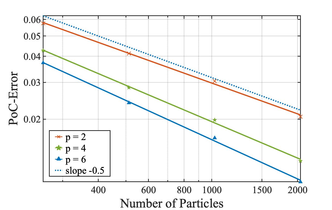
Figure 1: convergence rate of the PoC

Example 2.

In this example, we test the $L^{p}$ rate of PoC in different dimensions for $p=2,4,6$ and compare the findings to the theoretical upper bounds established by (11). For system (5)-(6), we make the following choices: Let $d\geq 2$, $x=(x_{1},...,x_{d})\in\mathbb{R}^{d}$, $(W_{t})_{0\leq t\leq T}$ is a 1-dim Brownian motion, the initial condition is a vector distributed according to $d$-independent $N(0,1)$-random variables, the coefficients are taken to be $a(x)=x-x^{3}=(x_{1}-x_{1}^{3},\dots,x_{d}-x_{d}^{3})^{\rm T}$,

$$\kappa(x,y)=y,\quad\zeta(x,y)= \left(\begin{array}[]{c}\sin(x_{1})+x_{2}+\cdots+x_{d}+y_{1}\\ x_{1}+\sin(x_{2})+\cdots+x_{d}+y_{2}\\ \cdots\\ x_{1}+x_{2}+\cdots+\sin(x_{d})+y_{d}\end{array}\right),$$

and $A(x)=\sin(x)=(\sin(x_{1}),\dots,\sin(x_{d})^{\rm T},B(x)=\cos(x)=(\cos(x_{1}),\dots,\cos(x_{d}))^{\rm T}$. We performed PoC rate tests in the sense of $L^{2}$, $L^{4}$ and $L^{6}$, respectively. When $p=2$, we simulated the equations for dimensions $d=2$ (then $p>d/2$), $d=4(p=d/2)$ and $d=6(p\in[2,d/2))$, when $p=4$, we simulated the equations for dimensions $d=4$ ($p>d/2$), $d=8(p=d/2)$ and $d=10(p\in[2,d/2))$, and when $p=6$, we simulated the equations for dimensions $d=4,12,14$. It can be found in Figures 2, 3 and 4 that the PoC rates observed numerically are all around $\mathcal{O}(N^{-1/2})$ and do not depend on the dimension of the solution.

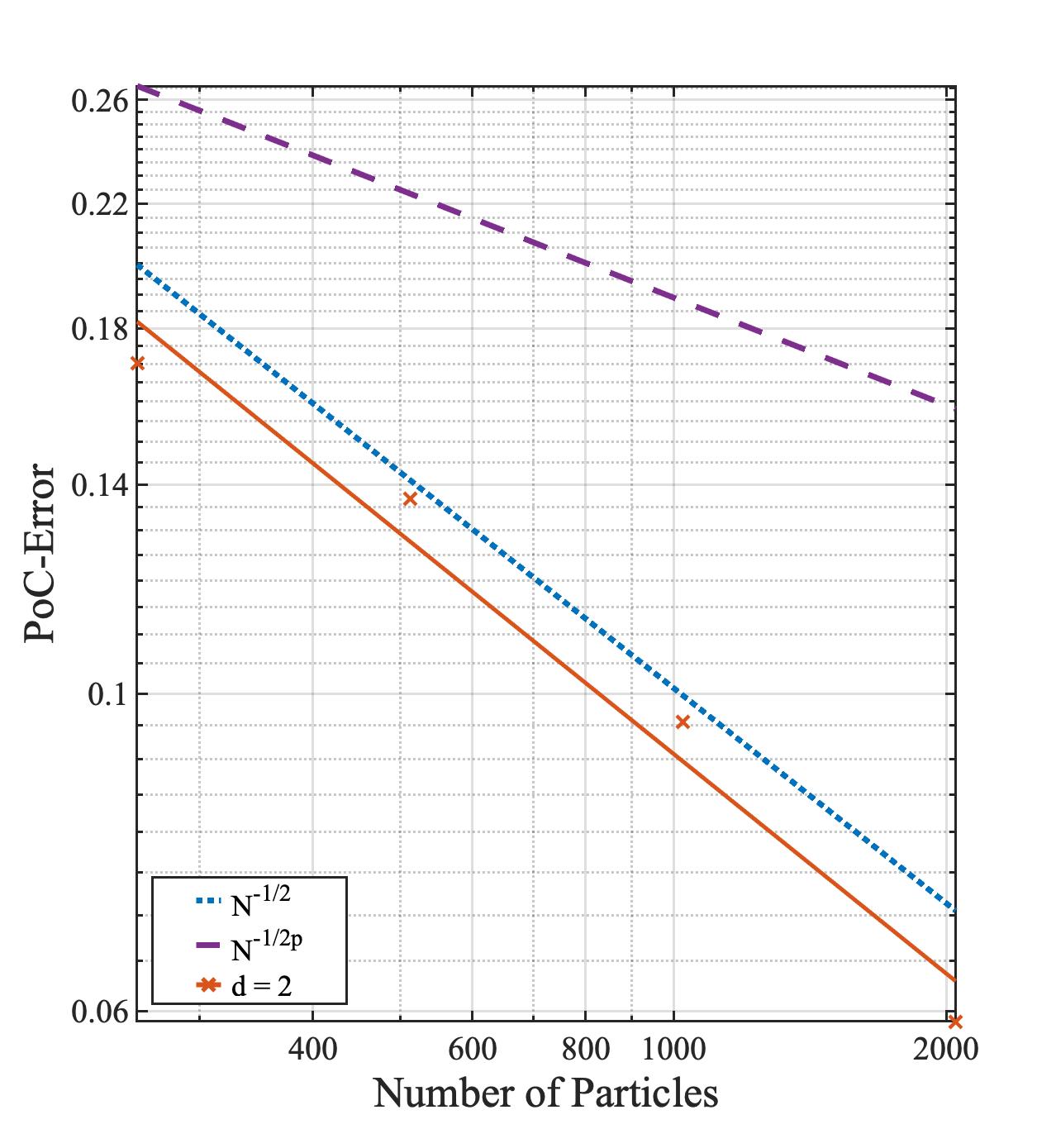
(a) d = 2

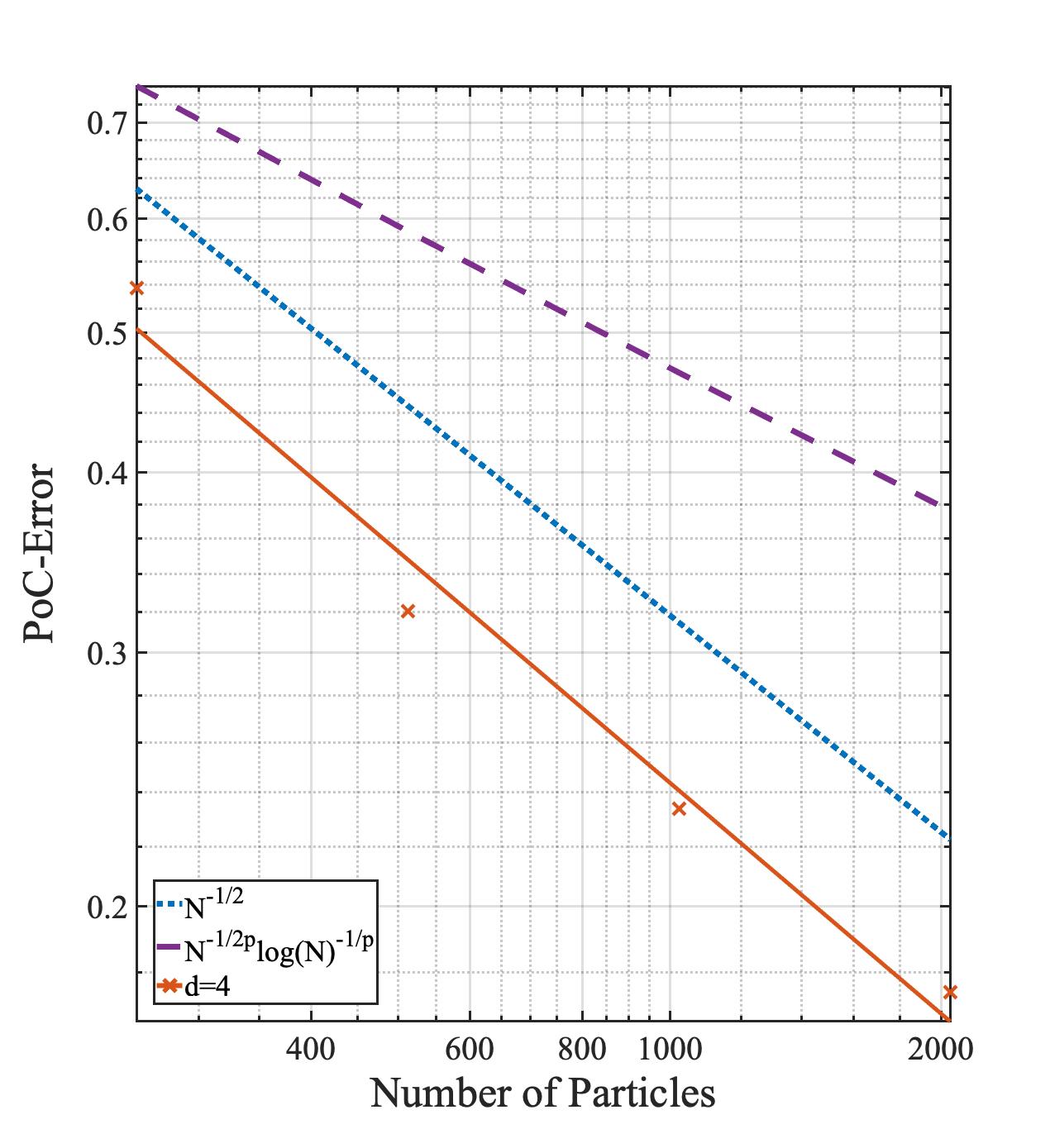
(b) d = 4

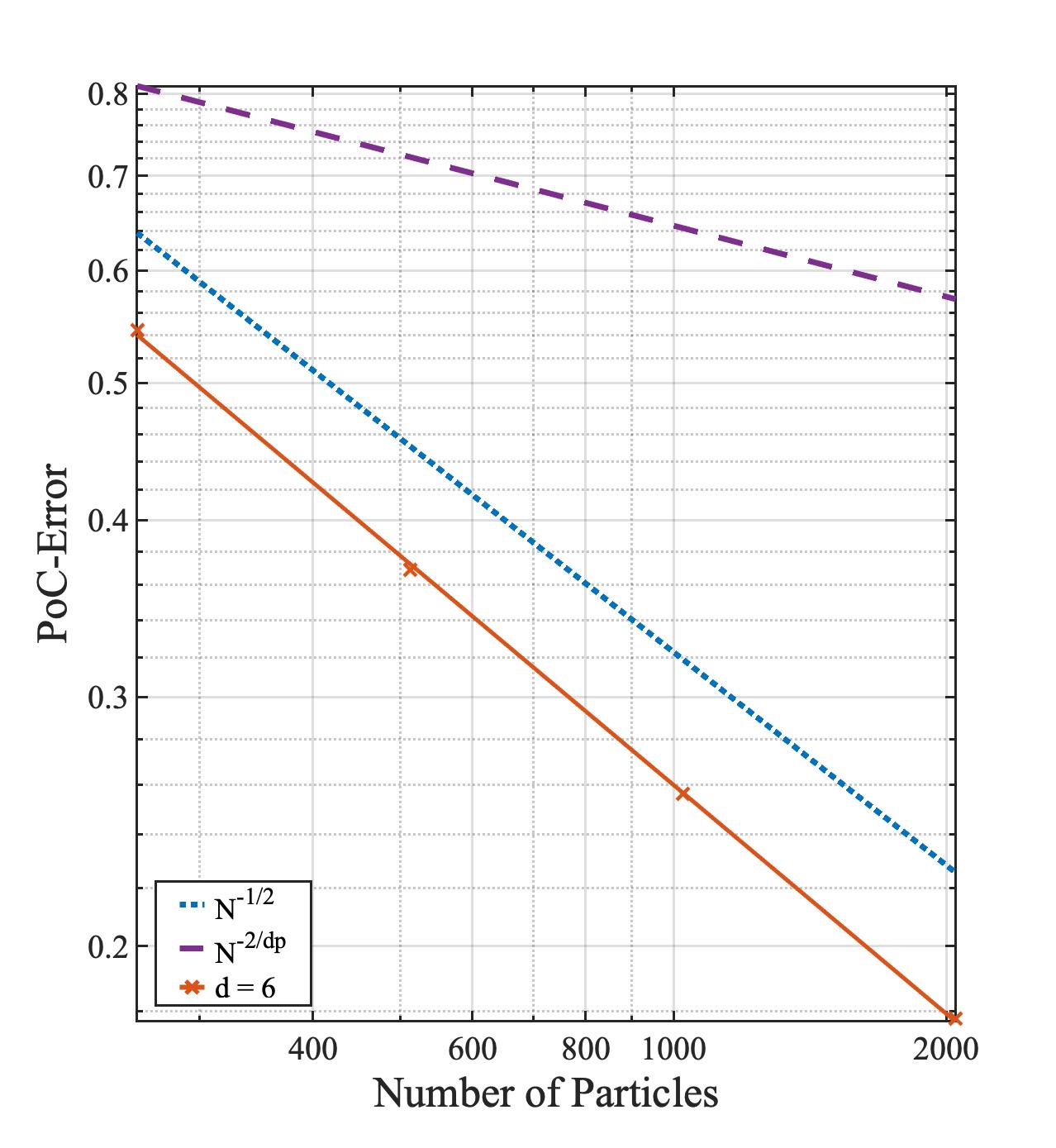
(c) d = 6

Figure 2: $L^{2}$ convergence rate of the PoC.

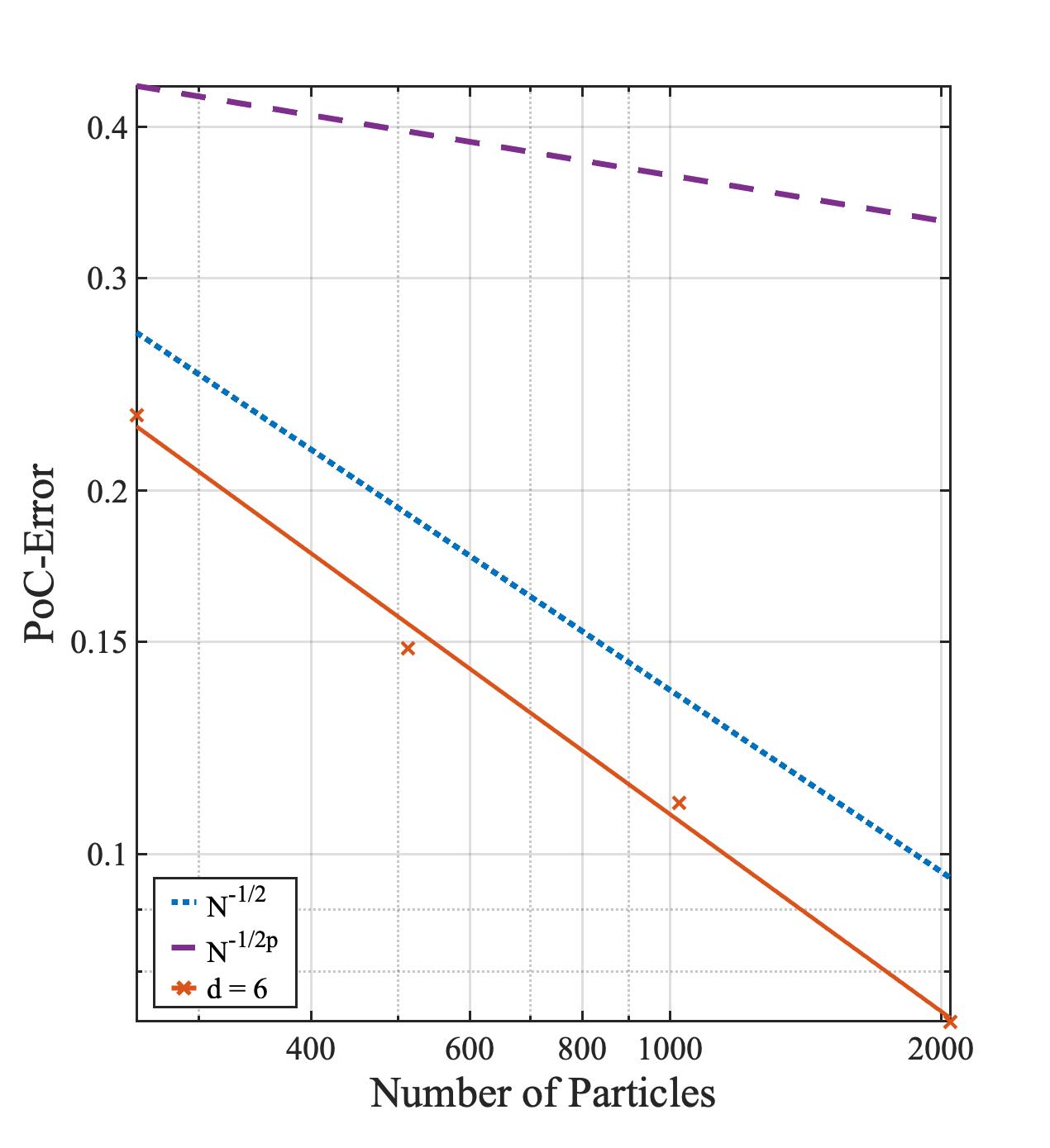
(a) d = 6

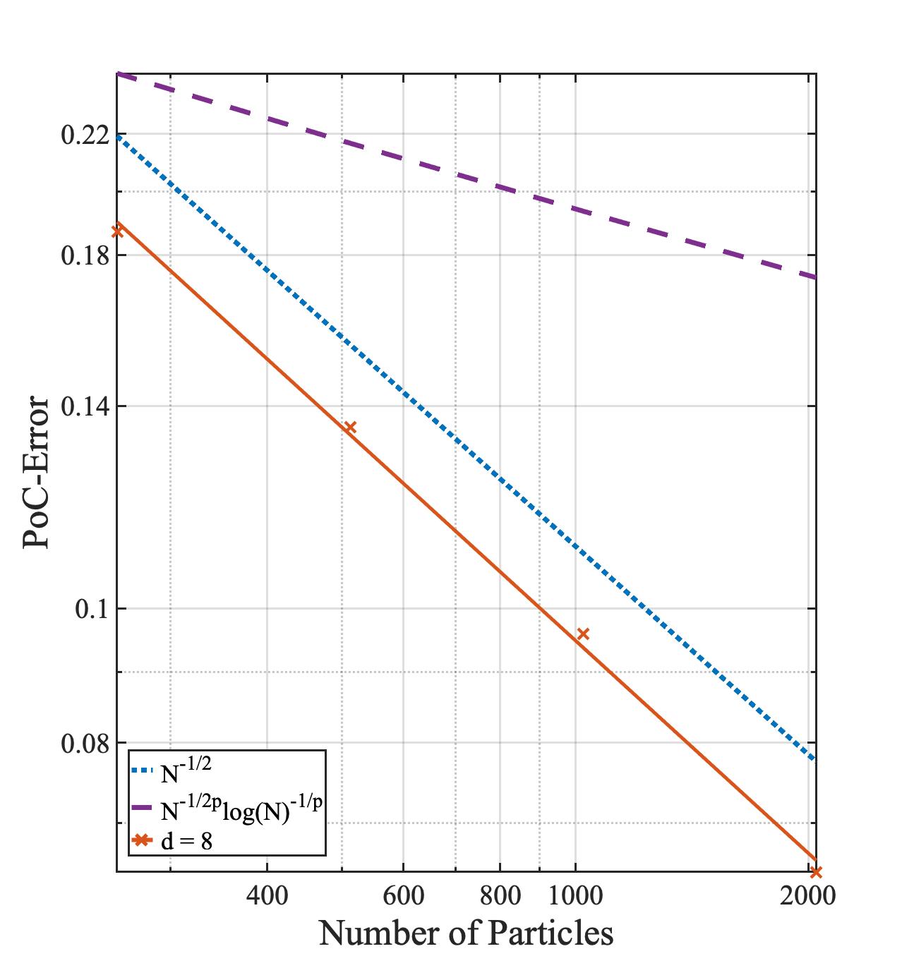
(b) d = 8

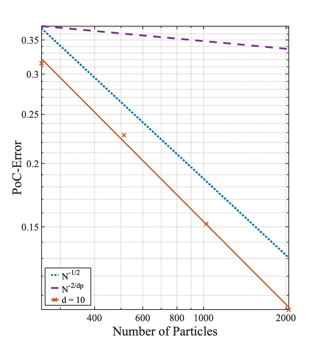
(c) d = 10

Figure 3: $L^{4}$ convergence rate of the PoC.

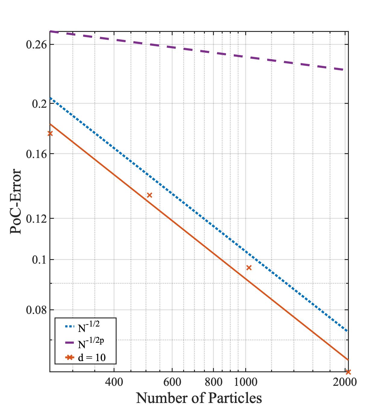
(a) d = 10

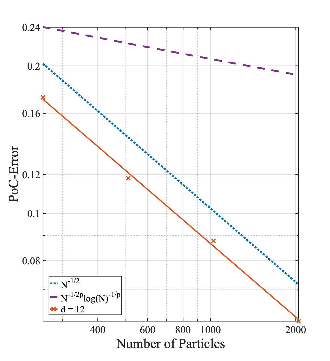
(b) d = 12

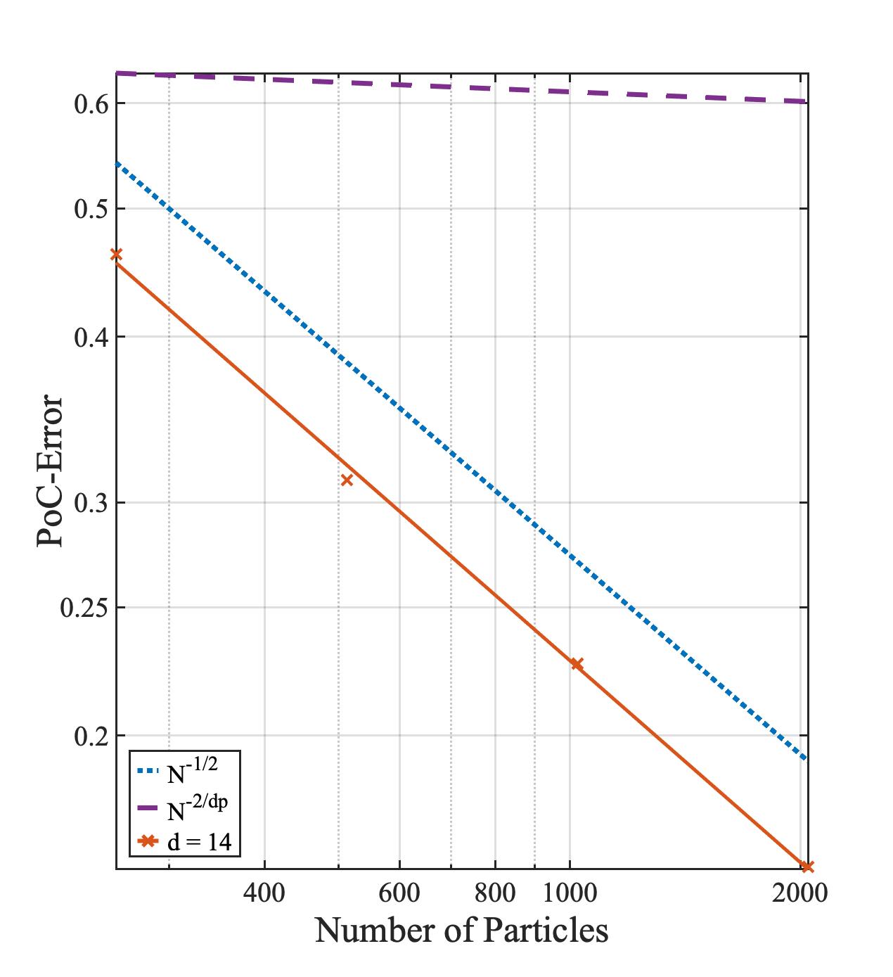
(c) d = 14

Figure 4: $L^{6}$ convergence rate of the PoC.

Appendix A Proof of Theorem 2.1

First, let us introduce some definitions for simplicity and give some lemmas.

For $x\in\mathbb{R}^{d}$, define

$$\hat{\kappa}(x):=\int_{\mathbb{R}^{d}}\kappa(x,y)\mu^{x}({\rm d}y),\quad\hat{\zeta}(x):=\int_{\mathbb{R}^{d}}\zeta(x,z)\mu^{x}({\rm d}z),$$

then (5) equals to

$$x_{t}^{i}=x_{0}^{i}+\int_{0}^{t}a(x_{s}^{i}){\rm d}s+\int_{0}^{t}A\left(\hat{\kappa}(x_{s}^{i})\right){\rm d}s+\int_{0}^{t}B\left(\hat{\zeta}(x_{s}^{i})\right){\rm d}W_{s}^{i}.$$ (15)

Correspondingly, for $i=1,2,\dots,N$ and $x^{i}\in\mathbb{R}^{d}$, define

$$\hat{\kappa}^{N}(x^{i}):=\frac{1}{N}\sum_{j=1}^{N}\kappa(x^{i},x^{j}),\quad\hat{\zeta}^{N}(x^{i}):=\frac{1}{N}\sum_{j=1}^{N}\zeta(x^{i},x^{j}),$$

then (7) equals to

$$X_{t}^{i,N,\delta}=x_{0}^{i}+\int_{0}^{t}\tilde{a}(X_{\delta_{s}}^{i,N,\delta}){\rm d}s+\int_{0}^{t}A\left(\hat{\kappa}^{N}(X_{\delta_{s}}^{i,N,\delta})\right){\rm d}s+\int_{0}^{t}B\left(\hat{\zeta}^{N}(X_{\delta_{s}}^{i,N,\delta})\right){\rm d}W_{s}^{i}.$$ (16)

Lemma A.1.

Let $p>2$, for any $t\in[0,T]$, it holds under Assumption 2.3 that

$$\mathbb{E}\left|\hat{\kappa}(x_{t}^{i})-\hat{\kappa}^{N}(x_{t}^{i})\right|^{p}\vee\mathbb{E}\left|\hat{\zeta}(x_{t}^{i})-\hat{\zeta}^{N}(x_{t}^{i})\right|^{p}\leq CN^{-p/2}.$$

Proof.

According to inequality (4), and the Rosenthal inequality (see [36]), we can deduce that

$$\mathbb{E}|\hat{\kappa}(x_{t}^{i})-\hat{\kappa}^{N}(x_{t}^{i})|^{p}=\mathbb{E}\left|\frac{1}{N}\sum_{j=1}^{N}\int_{\mathbb{R}^{d}}\left(\kappa(x_{t}^{i},y)-\kappa(x_{t}^{i},x_{t}^{j})\right)\mu_{t}^{x^{i}}({\rm d}y)\right|^{p}$$

$$\leq CN^{-p}\left(\mathbb{E}\left|\int_{\mathbb{R}^{d}}\left(\kappa(x_{t}^{i},y)-\kappa(x_{t}^{i},x_{t}^{i})\right)\mu_{t}^{x^{i}}({\rm d}y)\right|^{p}+\mathbb{E}\left|\sum_{j\neq i}\int_{\mathbb{R}^{d}}\left(\kappa(x_{t}^{i},y)-\kappa(x_{t}^{i},x_{t}^{j})\right)\mu_{t}^{x^{i}}({\rm d}y)\right|^{p}\right)$$

$$\leq CN^{-p}\mathbb{E}\left|\int_{\mathbb{R}^{d}}\left(\kappa(x_{t}^{i},y)-\kappa(x_{t}^{i},x_{t}^{i})\right)\mu_{t}^{x^{i}}({\rm d}y)\right|^{p}+CN^{-p}\sum_{j\neq i}\mathbb{E}\left|\int_{\mathbb{R}^{d}}\left(\kappa(x_{t}^{i},y)-\kappa(x_{t}^{i},x_{t}^{j})\right)\mu_{t}^{x^{i}}({\rm d}y)\right|^{p}$$

$$+CN^{-p}\left(\sum_{j\neq i}\mathbb{E}\left|\int_{\mathbb{R}^{d}}\left(\kappa(x_{t}^{i},y)-\kappa(x_{t}^{i},x_{t}^{j})\right)\mu_{t}^{x^{i}}({\rm d}y)\right|^{2}\right)^{p/2}.$$

Then, applying the Hölder inequality, Assumption 2.3 and Lemma 2.1, yields that

$$\mathbb{E}|\hat{\kappa}(x_{t}^{i})-\hat{\kappa}^{N}(x_{t}^{i})|^{p}$$

$$\leq CN^{-p}\mathbb{E}\int_{\mathbb{R}^{d}}\left|\kappa(x_{t}^{i},y)-\kappa(x_{t}^{i},x_{t}^{i})\right|^{p}\mu_{t}^{x^{i}}({\rm d}y)+CN^{-p}\sum_{j\neq i}\mathbb{E}\int_{\mathbb{R}^{d}}\left|\kappa(x_{t}^{i},y)-\kappa(x_{t}^{i},x_{t}^{j})\right|^{p}\mu_{t}^{x^{i}}({\rm d}y)$$

$$+CN^{-p}(N-1)^{p/2-1}\sum_{j\neq i}\mathbb{E}\int_{\mathbb{R}^{d}}\left|\kappa(x_{t}^{i},y)-\kappa(x_{t}^{i},x_{t}^{j})\right|^{p}\mu_{t}^{x^{i}}({\rm d}y)$$

$$\leq CN^{-p}\mathbb{E}\int_{\mathbb{R}^{d}}|y-x_{t}^{i}|^{p}\mu_{t}^{x^{i}}({\rm d}y)+C(N^{-p}+N^{-p/2-1})\sum_{j\neq i}\mathbb{E}\int_{\mathbb{R}^{d}}|y-x_{t}^{j}|^{p}\mu_{t}^{x^{i}}({\rm d}y)$$

$$\leq CN^{-p}\mathbb{E}\left(\mathbb{E}|x_{t}^{i}|^{p}+|x_{t}^{i}|^{p}\right)+C(N^{-p}+N^{-p/2-1})\sum_{j\neq i}\mathbb{E}\left(\mathbb{E}|x_{t}^{i}|^{p}+|x_{t}^{j}|^{p}\right)$$

$$\leq CN^{-p/2}(N^{-p/2}+N^{-p/2+1}+1)$$

$$\leq CN^{-p/2}.$$ (17)

Analogously we can also get

$$\mathbb{E}\left|\hat{\zeta}(x_{t}^{i})-\hat{\zeta}^{N}(x_{t}^{i})\right|^{p}\leq CN^{-p/2}$$

from Assumption 2.3. ∎

Lemma A.2.

Let $p>2$, for any $t\in[0,T]$, it holds under Assumptions 2.1, 2.3 and 2.4 that

$$\mathbb{E}|X_{t}^{i,N,\delta}-X_{\delta_{t}}^{i,N,\delta}|^{p}\leq C(t-\delta_{t})^{p/2}.$$

Proof.

Since $\delta_{t}=[t/\delta]\delta,\delta>0$, it is easy to know that $0\leq\delta_{t}\leq t$, then

$$X_{t}^{i,N,\delta}= X_{\delta_{t}}^{i,N,\delta}+\int_{\delta_{t}}^{t}\tilde{a}(X_{\delta_{s}}^{i,N,\delta}){\rm d}s+\int_{\delta_{t}}^{t}A\left(\int_{\mathbb{R}^{d}}\kappa(X_{\delta_{s}}^{i,N,\delta},y)\mu_{\delta_{s}}^{X,N,\delta}({\rm d}y)\right){\rm d}s$$

$$+\int_{\delta_{t}}^{t}B\left(\int_{\mathbb{R}^{d}}\zeta(X_{\delta_{s}}^{i,N,\delta},y)\mu_{\delta_{s}}^{X,N,\delta}({\rm d}y)\right){\rm d}W_{s}^{i}.$$

On the other hand, for $s\in[\delta_{t},t]$, since

$$[\delta_{t}/\delta]\delta\leq[s/\delta]\delta\leq[t/\delta]\delta,$$

and

$$[\delta_{t}/\delta]\delta=\left[\frac{[t/\delta]\delta}{\delta}\right]\delta=[t/\delta]\delta,$$

we can get that $\delta_{s}=\delta_{t}$. Hence, using (4), the B-D-G inequality, and Remark 2.1, we have

$$\mathbb{E}|X_{t}^{i,N,\delta}-X_{\delta_{t}}^{i,N,\delta}|^{p}$$

$$= \mathbb{E}\left|\int_{\delta_{t}}^{t}\tilde{a}(X_{\delta_{s}}^{i,N,\delta}){\rm d}s+\int_{\delta_{t}}^{t}A\left(\int_{\mathbb{R}^{d}}\kappa(X_{\delta_{s}}^{i,N,\delta},y)\mu_{\delta_{s}}^{X,N,\delta}({\rm d}y)\right){\rm d}s+\int_{\delta_{t}}^{t}B\left(\int_{\mathbb{R}^{d}}\zeta(X_{\delta_{s}}^{i,N,\delta},y)\mu_{\delta_{s}}^{X,N,\delta}({\rm d}y)\right){\rm d}W_{s}^{i}\right|^{p}$$

$$\leq C(t-\delta_{t})^{p}\mathbb{E}\left|\tilde{a}(X_{\delta_{t}}^{i,N,\delta})\right|^{p}+C(t-\delta_{t})^{p}\mathbb{E}\left|A\left(\int_{\mathbb{R}^{d}}\kappa(X_{\delta_{t}}^{i,N,\delta},y)\mu_{\delta_{t}}^{X,N,\delta}({\rm d}y)\right)\right|^{p}$$

$$+C(t-\delta_{t})^{p/2-1}\mathbb{E}\int_{\delta_{t}}^{t}\left|B\left(\int_{\mathbb{R}^{d}}\zeta(X_{\delta_{s}}^{i,N,\delta},y)\mu_{\delta_{s}}^{X,N,\delta}({\rm d}y)\right)\right|^{p}{\rm d}s$$

$$\leq C(t-\delta_{t})^{p}\mathbb{E}\left|\tilde{a}(X_{\delta_{t}}^{i,N,\delta})\right|^{p}+C(t-\delta_{t})^{p}+C(t-\delta_{t})^{p}\mathbb{E}\left|\int_{\mathbb{R}^{d}}\kappa(X_{\delta_{t}}^{i,N,\delta},y)\mu_{\delta_{t}}^{X,N,\delta}({\rm d}y)\right|^{p}$$

$$+C(t-\delta_{t})^{p/2}\mathbb{E}\left|\int_{\mathbb{R}^{d}}\zeta(X_{\delta_{s}}^{i,N,\delta},y)\mu_{\delta_{s}}^{X,N,\delta}({\rm d}y)\right|^{p}$$

$$\leq C(t-\delta_{t})^{p}\mathbb{E}\left|\tilde{a}(X_{\delta_{t}}^{i,N,\delta})\right|^{p}+C(t-\delta_{t})^{p}+C(t-\delta_{t})^{p}\mathbb{E}\int_{\mathbb{R}^{d}}\left|\kappa(X_{\delta_{t}}^{i,N,\delta},y)\right|^{p}\mu_{\delta_{t}}^{X,N,\delta}({\rm d}y)$$

$$+C(t-\delta_{t})^{p/2}\mathbb{E}\int_{\mathbb{R}^{d}}\left|\zeta(X_{\delta_{s}}^{i,N,\delta},y)\right|^{p}\mu_{\delta_{s}}^{X,N,\delta}({\rm d}y)$$

$$\leq C(t-\delta_{t})^{p}\mathbb{E}\left|\tilde{a}(X_{\delta_{t}}^{i,N,\delta})\right|^{p}+C(t-\delta_{t})^{p}+C(t-\delta_{t})^{p/2}\mathbb{E}\int_{\mathbb{R}^{d}}(|X_{\delta_{t}}^{i,N,\delta}|^{p}+|y|^{p})\mu_{\delta_{s}}^{X,N,\delta}({\rm d}y)$$

$$\leq C(t-\delta_{t})^{p/2}\left((t-\delta_{t})^{p/2}\mathbb{E}\left|\tilde{a}(X_{\delta_{t}}^{i,N,\delta})\right|^{p}+(t-\delta_{t})^{p/2}+\mathbb{E}|X_{\delta_{t}}^{i,N,\delta}|^{p}\right).$$

Since $t-\delta_{t}\leq t\leq T$, applying Assumption 2.4, it holds that

$$\mathbb{E}|X_{t}^{i,N,\delta}-X_{\delta_{t}}^{i,N,\delta}|^{p}\leq C(t-\delta_{t})^{p/2}.$$

∎

Proof of Theorem 2.1.

For any $i=1,2,\dots,N$, according to (15) and (16), we have

$$e_{t}^{i,N}:=x_{t}^{i}-X_{t}^{i,N,\delta} =\int_{0}^{t}\left(a(x_{s}^{i})-\tilde{a}(X_{\delta_{s}}^{i,N,\delta})\right){\rm d}s+\int_{0}^{t}\left(A\left(\hat{\kappa}(x_{s}^{i})\right)-A\left(\hat{\kappa}^{N}(X_{\delta_{s}}^{i,N,\delta})\right)\right){\rm d}s$$

$$\quad+\int_{0}^{t}\left(B\left(\hat{\zeta}(x_{s}^{i})\right)-B\left(\hat{\zeta}^{N}(X_{\delta_{s}}^{i,N,\delta})\right)\right){\rm d}W_{s}^{i}.$$

For any $i\in\{1,2,\dots,N\}$, applying the Itô formula, the Cauchy-Schwarz inequality, and Assumption 2.3, one has

$$|e_{t}^{i,N}|^{p}\leq p\int_{0}^{t}|e_{s}^{i,N}|^{p-2}\left\langle e_{s}^{i,N},a(x_{s}^{i})-\tilde{a}(X_{\delta_{s}}^{i,N,\delta})\right\rangle{\rm d}s+p\lambda_{2}\int_{0}^{t}|e_{s}^{i,N}|^{p-1}\left|\hat{\kappa}(x_{s}^{i})-\hat{\kappa}^{N}(X_{\delta_{s}}^{i,N,\delta})\right|{\rm d}s$$

$$+\frac{p(p-1)\lambda_{3}^{2}}{2}\int_{0}^{t}|e_{s}^{i,N}|^{p-2}\left|\hat{\zeta}(x_{s}^{i})-\hat{\zeta}^{N}(X_{\delta_{s}}^{i,N,\delta})\right|^{2}{\rm d}s$$

$$+p\lambda_{3}\int_{0}^{t}|e_{s}^{i,N}|^{p-1}\left|\hat{\zeta}(x_{s}^{i})-\hat{\zeta}^{N}(X_{\delta_{s}}^{i,N,\delta})\right|{\rm d}W_{s}^{i}$$

$$=: J_{1}+J_{2}+J_{3}+J_{4}.$$ (18)

Following Assumption 2.2 and the Young inequality, it is easy to see that

$$J_{1}\leq p\int_{0}^{t}|e_{s}^{i,N}|^{p-2}\left\langle e_{s}^{i,N},a(x_{s}^{i})-a(X_{s}^{i,N,\delta})\right\rangle{\rm d}s+p\int_{0}^{t}|e_{s}^{i,N}|^{p-1}|a(X_{s}^{i,N,\delta})-a(X_{\delta_{s}}^{i,N,\delta})|{\rm d}s$$

$$+p\int_{0}^{t}|e_{s}^{i,N}|^{p-1}|a(X_{\delta_{s}}^{i,N,\delta})-\tilde{a}(X_{\delta_{s}}^{i,N,\delta})|{\rm d}s$$

$$\leq C\int_{0}^{t}|e_{s}^{i,N}|^{p}{\rm d}s+C\int_{0}^{t}(1+|X_{s}^{i,N,\delta}|^{q}+|X_{\delta_{s}}^{i,N,\delta}|^{q})^{p}|X_{s}^{i,N,\delta}-X_{\delta_{s}}^{i,N,\delta}|^{p}{\rm d}s$$

$$+\int_{0}^{t}|a(X_{\delta_{s}}^{i,N,\delta})-\tilde{a}(X_{\delta_{s}}^{i,N,\delta})|^{p}{\rm d}s.$$ (19)

Similarly, we can also be deduced from the Young inequality and Assumption 2.1 that

$$J_{2}\leq p\lambda_{2}\int_{0}^{t}|e_{s}^{i,N}|^{p-1}\left(|\hat{\kappa}(x_{s}^{i})-\hat{\kappa}^{N}(x_{s}^{i})|+|\hat{\kappa}^{N}(x_{s}^{i})-\hat{\kappa}^{N}(X_{s}^{i,N,\delta})|+|\hat{\kappa}^{N}(X_{s}^{i,N,\delta})-\hat{\kappa}^{N}(X_{\delta_{s}}^{i,N,\delta})|\right){\rm d}s$$

$$\leq (p-1)\lambda_{2}\int_{0}^{t}|e_{s}^{i,N}|^{p}{\rm d}s+\lambda_{2}\int_{0}^{t}|\hat{\kappa}(x_{s}^{i})-\hat{\kappa}^{N}(x_{s}^{i})|^{p}{\rm d}s+\frac{\lambda_{2}}{N}\sum_{j=1}^{N}\int_{0}^{t}\left(|e_{s}^{i,N}|^{p}+|e_{s}^{j,N}|^{p}\right){\rm d}s$$

$$+\frac{\lambda_{2}}{N}\sum_{j=1}^{N}\int_{0}^{t}\left(|X_{s}^{j,N,\delta}-X_{\delta_{s}}^{i,N,\delta}|^{p}+|X_{s}^{j,N,\delta}-X_{\delta_{s}}^{j,N,\delta}|^{p}\right){\rm d}s,$$ (20)

and

$$J_{3}\leq C\int_{0}^{t}|e_{s}^{i,N}|^{p}{\rm d}s+C\int_{0}^{t}\left|\hat{\zeta}(x_{s}^{i})-\hat{\zeta}^{N}(x_{s}^{i})\right|^{p}{\rm d}s+\frac{C}{N}\sum_{j=1}^{N}\int_{0}^{t}\left(|e_{s}^{i,N}|^{p}+|e_{s}^{j,N}|^{p}\right){\rm d}s$$

$$+\frac{C}{N}\sum_{j=1}^{N}\int_{0}^{t}\left(|X_{s}^{j,N,\delta}-X_{\delta_{s}}^{i,N,\delta}|^{p}+|X_{s}^{j,N,\delta}-X_{\delta_{s}}^{j,N,\delta}|^{p}\right){\rm d}s.$$ (21)

Substituting (A)-(A) into (A), it gives that

$$|e_{t}^{i,N}|^{p}\leq C\int_{0}^{t}|e_{s}^{i,N}|^{p}{\rm d}s+C\int_{0}^{t}(1+|X_{s}^{i,N,\delta}|^{q}+|X_{\delta_{s}}^{i,N,\delta}|^{q})^{p}|X_{s}^{i,N,\delta}-X_{\delta_{s}}^{i,N,\delta}|^{p}{\rm d}s$$

$$+\int_{0}^{t}|a(X_{\delta_{s}}^{i,N,\delta})-\tilde{a}(X_{\delta_{s}}^{i,N,\delta})|^{p}{\rm d}s+C\int_{0}^{t}|\hat{\kappa}(x_{s}^{i})-\hat{\kappa}^{N}(x_{s}^{i})|^{p}{\rm d}s+\frac{C}{N}\sum_{j=1}^{N}\int_{0}^{t}|e_{s}^{j,N}|^{p}{\rm d}s$$

$$+\frac{C}{N}\sum_{j=1}^{N}\int_{0}^{t}\left(|X_{s}^{i,N,\delta}-X_{\delta_{s}}^{i,N,\delta}|^{p}+|X_{s}^{j,N,\delta}-X_{\delta_{s}}^{j,N,\delta}|^{p}\right){\rm d}s+C\int_{0}^{t}\left|\hat{\zeta}(x_{s}^{i})-\hat{\zeta}^{N}(x_{s}^{i})\right|^{p}{\rm d}s+J_{4}.$$

Then for any $T_{1}\in[0,T]$, since the $p$th moments of $x_{t}^{i}$ and $X_{t}^{i,N,\delta}$ are all bounded, we have

$$\mathbb{E}\left(\sup_{0\leq t\leq T_{1}}|e_{t}^{i,N}|^{p}\right)\leq C\int_{0}^{T_{1}}\mathbb{E}|e_{t}^{i,N}|^{p}{\rm d}t+C\int_{0}^{T_{1}}\left(\mathbb{E}(1+|X_{t}^{i,N,\delta}|^{q}+|X_{\delta_{t}}^{i,N,\delta}|^{q})^{2p}\mathbb{E}|X_{t}^{i,N,\delta}-X_{\delta_{t}}^{i,N,\delta}|^{2p}\right)^{1/2}{\rm d}t$$

$$+\int_{0}^{T_{1}}\mathbb{E}|a(X_{\delta_{t}}^{i,N,\delta})-\tilde{a}(X_{\delta_{t}}^{i,N,\delta})|^{p}{\rm d}t+C\int_{0}^{T_{1}}\mathbb{E}|\hat{\kappa}(x_{t}^{i})-\hat{\kappa}^{N}(x_{t}^{i})|^{p}{\rm d}t$$

$$+C\int_{0}^{T_{1}}\mathbb{E}|X_{t}^{i,N,\delta}-X_{\delta_{t}}^{i,N,\delta}|^{p}{\rm d}t+C\int_{0}^{T_{1}}\mathbb{E}\left|\hat{\zeta}(x_{t}^{i})-\hat{\zeta}^{N}(x_{t}^{i})\right|^{p}{\rm d}t$$

$$+C\mathbb{E}\sup_{0\leq t\leq T_{1}}\left(\int_{0}^{t}|e_{s}^{i,N}|^{p-1}\left|\hat{\zeta}(x_{s}^{i})-\hat{\zeta}^{N}(X_{s}^{i,N,\delta})\right|{\rm d}W_{s}^{i}\right).$$ (22)

Using the B-D-G inequality, similar to (A), it holds that

$$\mathbb{E}\sup_{0\leq t\leq T_{1}}\left(\int_{0}^{t}|e_{s}^{i,N}|^{p-1}\left|\hat{\zeta}(x_{s}^{i})-\hat{\zeta}^{N}(X_{\delta_{s}}^{i,N,\delta})\right|{\rm d}W_{s}^{i}\right)\leq C\mathbb{E}\left(\int_{0}^{T_{1}}|e_{t}^{i,N}|^{2p-2}|\hat{\zeta}(x_{t}^{i})-\hat{\zeta}^{N}(X_{\delta_{t}}^{i,N,\delta})|^{2}{\rm d}t\right)^{1/2}$$

$$\leq C\mathbb{E}\left(\sup_{0\leq t\leq T_{1}}|e_{t}^{i,N}|^{p}\int_{0}^{T_{1}}|e_{t}^{i,N}|^{p-2}|\hat{\zeta}(x_{t}^{i})-\hat{\zeta}^{N}(X_{\delta_{t}}^{i,N,\delta})|^{2}{\rm d}t\right)^{1/2}$$

$$\leq \frac{1}{2}\mathbb{E}\left(\sup_{0\leq t\leq T_{1}}|e_{t}^{i,N}|^{p}\right)+C\int_{0}^{T_{1}}\mathbb{E}|e_{t}^{i,N}|^{p}{\rm d}t+C\int_{0}^{T_{1}}\mathbb{E}\left|\hat{\zeta}(x_{t}^{i})-\hat{\zeta}^{N}(x_{t}^{i})\right|^{p}{\rm d}t+C\int_{0}^{T_{1}}\mathbb{E}|X_{t}^{i,N,\delta}-X_{\delta_{t}}^{i,N,\delta}|^{p}{\rm d}t.$$ (23)

Thus, combining (A) and (A), one has

$$\mathbb{E}\left(\sup_{0\leq t\leq T_{1}}|e_{t}^{i,N}|^{p}\right)\leq C\int_{0}^{T_{1}}\mathbb{E}|e_{t}^{i,N}|^{p}{\rm d}t+C\int_{0}^{T_{1}}\left(\mathbb{E}(1+|X_{t}^{i,N,\delta}|^{q}+|X_{\delta_{t}}^{i,N,\delta}|^{q})^{2p}\mathbb{E}|X_{t}^{i,N,\delta}-X_{\delta_{t}}^{i,N,\delta}|^{2p}\right)^{1/2}{\rm d}t$$

$$+\int_{0}^{T_{1}}\mathbb{E}|a(X_{\delta_{t}}^{i,N,\delta})-\tilde{a}(X_{\delta_{t}}^{i,N,\delta})|^{p}{\rm d}t+C\int_{0}^{T_{1}}\mathbb{E}|\hat{\kappa}(x_{t}^{i})-\hat{\kappa}^{N}(x_{t}^{i})|^{p}{\rm d}t$$

$$+C\int_{0}^{T_{1}}\mathbb{E}|X_{t}^{i,N,\delta}-X_{\delta_{t}}^{i,N,\delta}|^{p}{\rm d}t+C\int_{0}^{T_{1}}\mathbb{E}\left|\hat{\zeta}(x_{t}^{i})-\hat{\zeta}^{N}(x_{t}^{i})\right|^{p}{\rm d}t.$$ (24)

Substituting Lemmas A.1 and A.2 above into (A), using Assumption 2.4 again, it gives

$$\mathbb{E}\left(\sup_{0\leq t\leq T_{1}}|e_{t}^{i,N}|^{p}\right)\leq C\int_{0}^{T_{1}}\mathbb{E}|e_{t}^{i,N}|^{p}{\rm d}t+C\int_{0}^{T_{1}}(t-\delta_{t})^{p/2}\left(1+\left\{\mathbb{E}\left(\sup_{0\leq s\leq t}|X_{s}^{i,N,\delta}|^{2pq}\right)\right\}^{1/2}\right){\rm d}t$$

$$+CN^{-p/2}+\int_{0}^{T_{1}}\mathbb{E}|a(X_{\delta_{t}}^{i,N,\delta})-\tilde{a}(X_{\delta_{t}}^{i,N,\delta})|^{p}{\rm d}t$$

$$\leq C\int_{0}^{T_{1}}\mathbb{E}\left(\sup_{0\leq s\leq t}|e_{s}^{i,N}|^{p}\right){\rm d}t+CN^{-p/2}+C\int_{0}^{T_{1}}(t-\delta_{t})^{p/2}{\rm d}t$$

$$+C\int_{0}^{T_{1}}\mathbb{E}|a(X_{\delta_{t}}^{i,N,\delta})-\tilde{a}(X_{\delta_{t}}^{i,N,\delta})|^{p}{\rm d}t.$$

Therefore, it follows from the Gronwall inequality that

$$\mathbb{E}\left(\sup_{0\leq t\leq T_{1}}|e_{t}^{i,N}|^{p}\right)\leq CN^{-p/2}+C\sup_{0\leq t\leq T_{1}}(t-\delta_{t})^{p/2}+C\mathbb{E}\left(\sup_{0\leq t\leq T_{1}}|a(X_{t}^{i,N,\delta})-\tilde{a}(X_{t}^{i,N,\delta})|^{p}\right).$$

Then the assertion follows. ∎

References

- [1] J. Acebrón, L. Bonilla, C. Vicente, F. Ritort and R. Spigler, The Kuramoto model: A simple paradigm for synchronization phenomena, Rev. Modern Phys. 77 (1), 2005.
- [2] K. Bahlali, M. A. Mezerdi and B. Mezerdi, Stability of McKean-Vlasov stochastic differential equations and applications, Stoch. Dyn., 20, 2050007, 2020.
- [3] J. Baladron, D. Fasoli, O. Faugeras and J. Touboul, Mean-field description and propagation of chaos in networks of Hodgkin-Huxley and FitzHugh-Nagumo neurons, J. Math. Neurosci., 2: 1-50, 2012.
- [4] J. Bao, C. Reisinger, P. Ren and W. Stockinger, First-order convergence of Milstein schemes for McKean-Vlasov equations and interacting particle systems, Proc. A., 477 (2245): 20200258, 2021.
- [5] M. Bauer, T. Meyer-Brandis and F. Proske, Strong solutions of mean-field stochastic differential equations with irregular drift, Electron. J. Probab., 23: 1-35, 2018.
- [6] D. Belomestny and J. Schoenmakers, Projected particle methods for solving McKean-Vlasov stochastic differential equations, SIAM J. Numer. Anal., 56(6): 3169-3195, 2018.
- [7] M. Bossy and D. Talay, A stochastic particle method for the McKean-Vlasov and the Burgers equation, Math. Comp., 66(217): 157-192, 1997.
- [8] M. Bossy, O. Faugeras and D. Talay, Clarification and complement to “Mean-field description and propagation of chaos in networks of Hodgkin-Huxley and FitzHugh-Nagumo neurons”, J. Math. Neurosci., 5: 1-23, 2015.
- [9] R. Carmona, Lectures on BSDEs, Stochastic Control, and Stochastic Differential Games with Financial Applications, Volume 1 of Financial Mathematics, Society for Industrial and Applied Mathematics (SIAM), Philadelphia, PA, 2016.
- [10] R. Carmona and F. Delarue, Probabilistic Theory of Mean Field Games with Applications: I: Mean field FBSDEs, control, and games. Volume 83 of Probability Theory and Stochastic Modelling, Springer, 2018.
- [11] P. E. Chaudru de Raynal, Strong well posedness of McKean-Vlasov stochastic differential equations with Hölder drift, Stochastic Processes and their Applications, 130: 79-107, 2020.
- [12] X. Chen, G. Dos Reis and W. Stockinger, Wellposedness, exponential ergodicity and numerical approximation of fully super-linear MV-SDEs and associated particle systems, Electron. J. Probab., 30, Paper No. 1, 2025.
- [13] F. Delarue, D. Lacker and K. Ramanan, From the master equation to mean field game limit theory: A central limit theorem, Electron. J. Probab., 24(51): 1-54, 2019.
- [14] G. Dos Reis, S. Engelhardt and G. Smith, Simulation of MV-SDEs with super linear growth, IMA Journal of Numerical Analysis, 42: 874-922, 2022.
- [15] G. Dos Reis, W. Salkeld and J. Tugaut, Freidlin-Wentzell LDP in path space for McKean-Vlasov equations and the functional iterated logarithm law, Ann. Appl. Probab., 29(3): 1487-1540, 2019.
- [16] N. Fournier and A. Guillin, On the rate of convergence in Wasserstein distance of the empirical measure, Probab. Theory Related Fields ,162(3): 707-738, 2015.
- [17] S. Gao, Q. Guo, J. Hu and C. Yuan, Convergence rate in sense of tamed EM scheme for highly nonlinear neutral multiple-delay stochastic McKean-Vlasov equations, Journal of Computational and Applied Mathematics, 441, 115682, 2024.
- [18] Q. Guo, J. He and L. Li, Convergence analysis of an explicit method and its random batch approximation for the Mckean-Vlasov equations with non-globally Lipschitz conditions, ESAIM: Mathematical Modelling and Numerical Analysis, 58: 639-671, 2024.
- [19] D. J. Higham and P. E. Kloeden, An introduction to the numerical simulation of stochastic differential equations, SIAM, Philadelphia, PA, 2021.
- [20] M. Hutzenthaler, A. Jentzen and P. E. Kloeden, Strong convergence of an explicit numerical method for SDEs with nonglobally Lipschitz continuous coefficients, Ann. Appl. Probab. , 22(4): 1611-1641, 2012.
- [21] S. Jin, L. Li and J. Liu, Random batch methods (RBM) for interacting particle systems, J. Comput. Phys., 400, 108877, 2020.
- [22] S. Jin, L. Li and J. Liu, Convergence of the random batch method for interacting particles with disparate species and weights, SIAM J. Numer. Anal., 59(2): 746-768, 2021.
- [23] C. Kelly, G. J. Lord and F. Sun, Strong convergence of an adaptive time-stepping Milstein method for SDEs with monotone coefficients, BIT 63(2), Paper No. 33, 2023.
- [24] V. Kolokoltsov, Nonlinear Markov processes and kinetic equations, Cambridge Tracts in Mathematics, 182, Cambridge Univ. Press, Cambridge, 2010.
- [25] C. Kumar, Neelima, C. Reisinger and W. Stockinger, Well-posedness and tamed schemes for McKean-Vlasov equations with common noise, Ann. Appl. Probab., 32(5): 3283-3330, 2022.
- [26] Y. Li, X. Mao, Q. Song, F. Wu and G.Yin, Strong convergence of Euler-Maruyama schemes for McKean-Vlasov stochastic differential equations under local Lipschitz conditions of state variables, IMA Journal of Numerical Analysis, 43: 1001-1035, 2023.
- [27] Y. Liu, Particle method and quantization-based schemes for the simulation of the McKean-Vlasov equation, ESAIM: Mathematical Modelling and Numerical Analysis, 58, 571-612, 2024.
- [28] X. Mao, The truncated Euler-Maruyama method for stochastic differential equations, J. Comput. Appl. Math. 290: 370-384, 2015.
- [29] X. Mao, Convergence rates of the truncated Euler-Maruyama method for stochastic differential equations, J. Comput. Appl. Math. 296: 362-375, 2016.
- [30] N. Martzel and C. Aslangul, Mean-field treatment of the many-body Fokker-Planck equation, J. Phys. A: Math. General, 34: 11225, 2001.
- [31] H. McKean Jr., A class of Markov processes associated with nonlinear parabolic equations, Proc. Nat. Acad. Sci. U.S.A., 56: 1907-1911, 1966.
- [32] H. McKean Jr., Propagation of chaos for a class of non-linear parabolic equations, in Stochastic Differential Equations (Lecture Series in Differential Equations, Session 7, Catholic Univ. 1967), 41-57, 1967.
- [33] S. Méléard. Asymptotic behaviour of some interacting particle systems; McKean-Vlasov and Boltzmann models, In Probabilistic models for nonlinear partial differential equations, pages 42-95. Springer, 1996.
- [34] Y. Mishura and A. Veretennikov, Existence and uniqueness theorems for solutions of McKean-Vlasov stochastic equations, Theory Probab. Math. Stat., 103: 59-101, 2020.
- [35] C. Reisinger and W. Stockinger An adaptive Euler-Maruyama scheme for MV-SDEs with super-linear growth and application to the mean-field FitzHugh-Nagumo model, Journal of Computational and Applied Mathematics, 400: 113725, 2022.
- [36] H. Rosenthal, On the subspaces of spanned by sequences of independent random variables, Israel Journal of Mathematics, 8: 273-303, 1970.
- [37] S. Sabanis, A note on tamed Euler approximations, Electron. Commun. Probab. 18(47), 2013.
- [38] A. Sznitman, Topics in propagation of chaos. In Ecole d’Eté de Probabilités de Saint-Flour XIX–1989, Berlin: Springer, 165-251, 1991.
- [39] L. Szpruch and A. Tse, Antithetic multilevel sampling method for nonlinear functionals of measure, Ann. Appl. Probab., 31(3):1100-1139, 2021.
- [40] F. Wang, Distribution dependent SDEs for Landau type equations, Stochastic Process. Appl., 128: 595-621, 2018.
- [41] F. Wu, F. Xi and C. Zhu, On a class of McKean-Vlasov stochastic functional differential equations with applications, Journal of Differential Equations, 371: 31-49, 2023.
- [42] X. Wang and S. Gan, The tamed Milstein method for commutative stochastic differential equations with non-globally Lipschitz continuous coefficients, J. Difference Equ. Appl. 19(3): 466–490, 2013.
- [43] J. Zhang, Topics in McKean-Vlasov equations: Rank-based dynamics and Markovian projection with applications in finance and stochastic control, Ph.D. thesis, Princeton University, 2021.