Exploiting Partial Assignments
in Optimization Modulo Theories

Abstract

Optimization Modulo Theories (OMT) extends Satisfiability Modulo Theories (SMT) with the task of optimizing some objective function(s). In OMT solvers, a CDCL-based SMT solver enumerates theory-satisfiable total truth assignments, and a theory-specific procedure finds an optimum model for each of them; the current optimum is then used to tighten the search space for the next assignments, until no better solution is found.

In this paper, we analyze the role of truth-assignment enumeration in OMT. First, we spotlight that the enumeration of total truth assignments is suboptimal, since they may over-restrict the search space for the optimization procedure, whereas using partial truth assignments instead can improve the effectiveness of the optimization. Second, we propose some reduction techniques for better exploiting partial assignments in the OMT context. We implemented these techniques in the OptiMathSAT solver, and conducted an experimental evaluation on $\text{OMT}(\mathcal{LRA})$ benchmarks. The results support the efficiency and effectiveness of our approach.

1 Introduction

Satisfiability Modulo Theories (SMT) is the problem of deciding the satisfiability of a logical formula w.r.t. some background theory, such as linear and nonlinear arithmetic, bit-vectors, arrays, or uninterpreted functions [2]. Many SMT-encodable problems also require the capability of finding models that are optimal w.r.t. some objective functions. These problems are grouped under the term Optimization Modulo Theories (OMT) [22, 28, 5]. OMT has been successfully applied to a wide range of problems, such as verification of timed and hybrid systems [28, 13], numeric [15] and temporal planning [23, 24], optimal scheduling [6], constrained goal modelling [21], hybrid machine learning [34], GAS optimization for smart contracts [1], and optimum encodings for quantum annealing [3, 9], establishing OMT solvers as powerful tools for solving complex constraint optimization problems in various domains.

OMT solving.

A general OMT-solving strategy [22, 28, 29] consists in performing a sequence of incremental SMT calls, progressively tightening the range of values for the objective function. Specifically, an SMT solver is used to enumerate $\mathcal{T}$-satisfiable truth assignments that propositionally satisfy the problem formula $\varphi$. For each such truth assignment, a $\mathcal{T}$-optimizer finds a $\mathcal{T}$-model of optimum cost within it. A constraint is then added to the formula to tighten the upper bound for the cost of the optimum model, and the search continues until the formula is found unsatisfiable. Besides optimal solving, an important feature of OMT solvers is the ability to provide the user with a good-enough solution within a given time budget. This capability, known as anytime OMT solving, is especially valuable in industrial applications where finding the optimum solution may be computationally impractical, and it is rather more important to obtain high-quality solutions quickly.

OMT techniques have been developed for $\mathcal{LRA}$ [5, 29], $\mathcal{LIA}$ [5, 30], $\mathcal{NRA}$ [4], $\mathcal{NIA}$ [4], $\mathcal{BV}$ [20, 36], and $\mathcal{FP}$ [36]. Also, OMT has been extended to deal with multiple objectives including lexicographic OMT [5, 30], boxed OMT [5, 16, 30], min-max OMT [31], and Pareto OMT [5]. Recently, a Generalized OMT calculus has been proposed, extending the definition to objectives over partially ordered sets [38].

Partial assignments enumeration SMT.

The problem of truth assignment enumeration has been studied in recent years, mainly in the context of SAT and SMT enumeration (AllSAT and AllSMT). Typically, enumeration algorithms [14, 12, 11, 33] rely their efficiency on the enumeration of partial assignments to reduce both the number of enumerated assignments and the computational time by up to an exponential factor. Several techniques have been proposed to find short satisfying partial assignments starting from a total assignment, trading off efficiency for effectiveness (e.g., [19, 26, 35]). Also, the impact of CNF-ization on the effectiveness of partial assignment reduction has been recently studied in [18, 32].

Contributions.

In this paper, we study the applicability of enumeration-based techniques to OMT solving, and, in particular, the usage of partial truth assignment reduction to improve the effectiveness and efficiency of OMT solving. First, we notice that OMT solvers typically invoke the $\mathcal{T}$-optimizer on total truth assignments, and we spotlight how this can be suboptimal in many cases. Second, we propose some ways to exploit partial truth assignments in OMT solving, tailoring existing techniques to the OMT context. We show through an empirical evaluation over $\text{OMT}(\mathcal{LRA})$ benchmarks that these strategies can improve both the efficiency of OMT optimal solving and the quality of obtained solutions for anytime solving.

Organization.

The rest of the paper is organized as follows. In §2, we provide the necessary background on SMT and OMT solving. In §3, we analyze the role of total and partial truth assignments in OMT solving. In §4, we propose two strategies to exploit partial truth assignments in OMT solving. In §5, we present an experimental evaluation of the proposed strategies over $\text{OMT}(\mathcal{LRA})$ benchmarks. Finally, in §6, we conclude the paper and discuss future work.

2 Background

Notation and terminology.

We assume the standard setting with quantifier-free first-order formulas, and the standard notions of theory, satisfiability, logical consequence. We assume the reader is familiar with these notions and with the lazy CDCL-based SMT-solving approach, and refer to [2] for a comprehensive introduction to SMT.

In this paper, we denote SMT formulas by $\varphi$, theories by $\mathcal{T}$, variables by $x,y$, atoms by $\alpha$, truth assignments by $\mu,\eta$, and models by $\mathcal{M}$; all symbols possibly with subscripts or superscripts. We denote by $Atoms(\varphi)$ the set of atoms occurring in a formula $\varphi$.

2.1 Satisfiability Modulo Theories

Given a first-order theory $\mathcal{T}$, a $\mathcal{T}$-atom is any atomic formula built over the signature of $\mathcal{T}$. A $\mathcal{T}$-literal is a $\mathcal{T}$-atom or its negation. A $\mathcal{T}$-formula is either a $\mathcal{T}$-literal or a combination of formulas by means of standard Boolean operators. From now on, we assume every formula is in Conjunctive Normal Form (CNF), i.e., it is a conjunction ($\wedge$) of clauses, where each clause is a disjunction ($\vee$) of literals. (If it is not, then it can be easily converted into CNF by applying the standard transformations [25, 37]).

Satisfiability Modulo Theories (SMT) is the problem of deciding the satisfiability of a first-order formula w.r.t some first-order theory $\mathcal{T}$, or combination of first-order theories $\mathcal{T}_{1}\cup\mathcal{T}_{2}$. A formula is $\mathcal{T}$-satisfiable if it is satisfiable in a model of $\mathcal{T}$ (also written as T-model). Popular theories include linear and nonlinear arithmetic over the reals or integers ($\mathcal{LRA}$, $\mathcal{NRA}$, $\mathcal{LIA}$, and $\mathcal{NIA}$, respectively), bit-vectors ($\mathcal{BV}$), and floating-point ($\mathcal{FP}$).

Lazy SMT-solving.

Given a formula $\varphi$ with $Atoms(\varphi)\stackrel{{\scriptstyle\text{\scalebox{0.7}{def}}}}{{=}}\{\alpha_{1},\ldots,\alpha_{n}\}$, a truth assignment $\mu:Atoms(\varphi)\to\{\top,\bot\}$ is a mapping from atoms in $\varphi$ to truth values. A partial truth assignment is a partial mapping, and a total truth assignment is a total mapping. We represent a truth assignment $\mu$ also as a conjunction of literals $\bigwedge_{\mu(\alpha_{i})=\top}\alpha_{i}\wedge\bigwedge_{\mu(\alpha_{i})=\bot}\neg\alpha_{i}$. We say that $\mu$ propositionally satisfies $\varphi$ iff $\mu$ satisfies all clauses in $\varphi$.

The CDCL($\mathcal{T}$) algorithm [17] is based on the so-called lazy approach to SMT (see e.g., [27, 2]), which exploits the fact that a $\mathcal{T}$-formula $\varphi$ is $\mathcal{T}$-satisfiable iff there exists a truth assignment $\mu$ that propositionally satisfies $\varphi$ and $\mu$ is $\mathcal{T}$-satisfiable. It combines a CDCL-based SAT-solver with a $\mathcal{T}$-specialized decision procedure called $\mathcal{T}$-solver to decide the consistency of a set of $\mathcal{T}$-constraints. Whenever the SAT-solver finds a truth assignment $\mu$ propositionally satisfying $\varphi$, it invokes the $\mathcal{T}$-solver to check the $\mathcal{T}$-satisfiability of $\mu$. If $\mu$ is $\mathcal{T}$-satisfiable, then the $\mathcal{T}$-solver returns a model $\mathcal{M}$, that is also a model of $\varphi$. Otherwise, the $\mathcal{T}$-solver returns a subset of $\mu$ that causes the $\mathcal{T}$-unsatisfiability, which is learned by the SAT-solver and used in subsequent iterations to prune the search space.

To maximize efficiency, most $\mathcal{T}$-solvers can be called incrementally via a stack-based interface, keeping the status of the search between calls. E.g., [10] proposed an efficient incremental $\mathcal{LRA}$-solver, based on a variant of the Simplex algorithm designed to be integrated within a lazy SMT framework. The combination of theories can be handled efficiently by delayed theory combination [7].

Another important feature of CDCL-based SMT solvers is that they provide a stack-based incremental interface, allowing to push and pop clauses and incrementally check the satisfiability of the formula conjoined with the pushed clauses, maintaining most of the learned information between calls.

2.2 Optimization Modulo Theories

Let $\mathcal{T}$ be a theory admitting some total order relation “$\leq$” over its domain, let $\varphi$ be a $\mathcal{T}$-formula, and let $\mathsf{cost}$ be a $\mathcal{T}$-term which we call objective function. Optimization Modulo Theories (OMT) is the problem of finding a model for $\varphi$ that makes the value of $\mathsf{cost}$ minimum according to the order given by $\leq$ (maximization is dual) [4, 28]. To simplify the presentation, we focus on minimization, but the same concepts apply to maximization as well. Notice that, in general, $\varphi$ can be built on a combination of $\mathcal{T}$ with other theories [28]. To simplify the explanation and the notation, we refer to one single theory.

Example 1

Consider the $\mathcal{LRA}$-formula on the real variables $x,y$:

$$\begin{array}[]{ll}\varphi\stackrel{{\scriptstyle\text{\scalebox{0.7}{def}}}}{{=}}&((2x-3y\leq 6)\vee(x\leq 4))\wedge\\ &((y\leq 2)\vee(y\leq-3x+9)\vee(x<-2)).\end{array}$$ (1)

$\varphi$ is $\mathcal{LRA}$-satisfiable, e.g., the $\mathcal{LRA}$-model $\mathcal{M}\stackrel{{\scriptstyle\text{\scalebox{0.7}{def}}}}{{=}}\{{x\mapsto{}3,y\mapsto{}0}\}$ satisfies $\varphi$.

Consider the $\text{OMT}(\mathcal{LRA})$ problem $\langle{\varphi},{\mathsf{cost}}\rangle$ where $\varphi$ is the $\mathcal{LRA}$-formula in (1), and $\mathsf{cost}\stackrel{{\scriptstyle\text{\scalebox{0.7}{def}}}}{{=}}-2x$. Then the model $\mathcal{M}\stackrel{{\scriptstyle\text{\scalebox{0.7}{def}}}}{{=}}\{{x\mapsto{}3,y\mapsto{}0}\}$ has $\mathsf{cost}=-6$. A better model of $\varphi$ is, e.g., $\mathcal{M}^{\prime}\stackrel{{\scriptstyle\text{\scalebox{0.7}{def}}}}{{=}}\{{x\mapsto{}6,y\mapsto{}2}\}$, that has $\mathsf{cost}=-12$. This model is also the model of $\varphi$ with minimum cost.

Lazy OMT solving.

A general optimization strategy implemented by state-of-the-art OMT solvers is the so-called linear-search strategy [22, 28, 29]. It consists in solving a sequence of SMT problems where the space of feasible solutions is progressively tightened by learning unit clauses in the form $(\mathsf{cost}<{\sf ub})$, ${\sf ub}$ being the currently-known upper bound for $\mathsf{cost}$. At each iteration, the solver can either find a model $\mathcal{M}$ whose value of $\mathsf{cost}$ is smaller than ${\sf ub}$, or detect the unsatisfiability of the current formula. In the first case, the solver invokes a $\mathcal{T}$-specific procedure, called $\mathcal{T}$-minimizer, to find an optimum model $\mathcal{M}^{\prime}$ within the truth assignment induced by $\mathcal{M}$. E.g., a $\mathcal{LRA}$-minimizer [28] can be implemented as a simple extension of the Simplex-based $\mathcal{LRA}$-solver [10, 28]. Then, the new upper bound is set to the value assigned to $\mathsf{cost}$ by $\mathcal{M}^{\prime}$, and the search continues. In the second case, the formula has no models with $\mathsf{cost}$ lower than ${\sf ub}$, and the search terminates as the last model found is optimum.

Alternatively, the solver could also follow a binary-search strategy [28]. In this case, a lower and upper bound ${\sf lb}$ and ${\sf ub}$ are kept s.t. the optimum model lies in the interval $\mathopen{(}{\sf lb}{},{\sf ub}{}\mathclose{]}$. At each iteration, an intermediate value $\mathsf{pivot}{}\in\mathopen{(}{\sf lb}{},{\sf ub}{}\mathclose{]}$ is chosen, and the solver checks if there exists a model with $\mathsf{cost}$ lower than $\mathsf{pivot}$. If so, $\mathsf{pivot}$ becomes the new upper bound, otherwise, it becomes the new lower bound. The search terminates when ${\sf lb}$ and ${\sf ub}$ are equal, and the last model found is optimum. (In continuous domains, e.g., $\text{OMT}(\mathcal{LRA})$, to guarantee termination, it is necessary to interleave binary-search steps with a linear-search step [28]). In this paper, we focus on the linear-search strategy, but the analysis applies to the binary-search strategy as well.

The lazy OMT solving approach allows for an anytime behavior, i.e., we can interrupt the search at any time and return the best model found so far.

2.3 SAT and SMT Enumeration

1: $\mu\leftarrow\eta$

2: for $\ell\in\mu$ do

3:  if $\mu\setminus\{{\ell}\}$ satisfies all clauses in $\varphi$ then

4:   $\mu\leftarrow\mu\setminus\{{\ell}\}$

5: return  $\mu$

Algorithm 1 reduce-assignment($\varphi,\eta$) Input: CNF formula $\varphi$, $\mathcal{T}$-satisfiable total truth assignment $\eta$ satisfying $\varphi$ Output: Reduced (minimal) partial truth assignment $\mu\subseteq\eta$ satisfying $\varphi$

SAT enumeration (AllSAT) is the problem of finding all the truth assignments that propositionally satisfy a propositional formula. SMT enumeration (AllSMT) is the problem of finding all $\mathcal{T}$-satisfiable truth assignments that propositionally satisfy a $\mathcal{T}$-formula. Since a partial assignment can be extended to $2^{k}$ total truth assignments, $k$ being the number of unassigned atoms, finding short partial truth assignments is a key point in reducing both the number of enumerated truth assignments and the computational time by up to an exponential factor.

Many enumeration algorithms find total truth assignments, and then extract partial truth assignments from them by some reduction procedure. A basic reduction procedure is illustrated in Algorithm˜1. It consists in iteratively dropping literals one-by-one from the truth assignment, checking if it still satisfies the formula. The resulting partial assignment is minimal, i.e., it cannot be further reduced without violating the satisfaction of the formula. Notice that the order in which literals are dropped can have a significant impact on the effectiveness of the reduction procedure.

3 An Analysis of Enumeration in OMT

As described in §2.2, a basic OMT solving schema involves the interaction of a combinatorial and a theory-specific optimization components. In the combinatorial component, a SMT solver enumerates $\mathcal{T}$-satisfiable truth assignments that propositionally satisfy the problem formula $\varphi$ conjoined with increasingly tighter bounds on the cost of the optimum solution. In the theory-specific component, a $\mathcal{T}$-minimizer finds a $\mathcal{T}$-model of minimum cost within the constraints imposed by the given truth assignment. This model is then used to tighten the upper bound for the cost of the optimum model and continue the search, until the formula is found unsatisfiable.

Since the enumeration is based on the CDCL($\mathcal{T}$) schema [17], these truth assignments are typically total, i.e., they assign a truth value to each atom of the formula. However, we point out that total truth assignments can often over-constrain the search space for the optimum model, whereas relying on partial truth assignments can be much more effective. Intuitively, by removing from the current satisfying truth assignment $\mathcal{T}$-constraints that are not strictly necessary for the propositional satisfaction of the formula, we enlarge the area within which the optimum model is searched, thus increasing the chances of finding a better optimum model. This means that the solver can add a tighter upper bound to the cost of the global optimum, potentially reducing the number of search iterations needed to find it, and consequently the overall solving time. Moreover, this improvement can be crucial for anytime OMT solving, as it allows the solver to converge faster to better solutions within the given time limit.

We illustrate this idea in the following example.

(a) Total assignment $\mu$ (2)

(b) Partial assignment $\mu^{\prime}$ (3)

(c) Partial assignment $\mu^{\prime\prime}$ (4)

Figure 1: Graphical representation of Example˜2. For each step, the half-planes representing the constraints in the truth assignment are delimited by dashed lines and colored in grey. The intersection of these constraints is colored in blue, with a gradient that follows the value of $\mathsf{cost}$ (the lower the value of $\mathsf{cost}$, the more intense the color), and the red dot represents the optimum model found within this region.

Example 2

Consider the $\text{OMT}(\mathcal{LRA})$ problem $\langle{\varphi},{\mathsf{cost}}\rangle$ where $\varphi$ is the formula in (1) in Example˜1, and $\mathsf{cost}\stackrel{{\scriptstyle\text{\scalebox{0.7}{def}}}}{{=}}-2x$. Consider the following scenario, which is graphically represented in Figure˜1. Consider the $\mathcal{LRA}$-satisfiable total truth assignment that propositionally satisfies $\varphi$:

$$\mu\stackrel{{\scriptstyle\text{\scalebox{0.7}{def}}}}{{=}}\{{(2x-3y\leq 6),(y\leq 2),\neg(x<-2),(y\leq-3x+9),(x\leq 4)}\}.$$ (2)

The optimum model of $\mu$ is $\{{x\mapsto{}3,y\mapsto{}0}\}$ with $\mathsf{cost}=-6$ (Figure˜1(a)). We notice, however, that, e.g., the constraint $(y\leq-3x+9)$ is not strictly necessary for propositionally satisfying $\varphi$, as $\varphi$ is satisfied also by:

$$\mu^{\prime}\stackrel{{\scriptstyle\text{\scalebox{0.7}{def}}}}{{=}}\mu\setminus\{{(y\leq-3x+9)}\}=\{{(2x-3y\leq 6),(y\leq 2),\neg(x<-2),(x\leq 4)}\}.$$ (3)

The optimum model of $\mu^{\prime}$ is $\{{x\mapsto{}4,y\mapsto{}2/3}\}$ with $\mathsf{cost}=-8$ (Figure˜1(b)). If we further remove the unnecessary constraint $(x\leq 4)$, then we obtain

$$\mu^{\prime\prime}\stackrel{{\scriptstyle\text{\scalebox{0.7}{def}}}}{{=}}\mu^{\prime}\setminus\{{(x\leq 4)}\}=\{{(2x-3y\leq 6),(y\leq 2),\neg(x<-2)}\}$$ (4)

with optimum model $\{{x\mapsto{}6,y\mapsto{}2}\}$ and $\mathsf{cost}=-12$ (Figure˜1(c)). Finally, we could remove either $\neg(x<-2)$ or $(y\leq 2)$. In the first case, we would obtain a partial truth assignment with the same optimum model as $\mu^{\prime\prime}$, since the constraint does not “oppose” to the optimization of $\mathsf{cost}$ in $\mu^{\prime\prime}$. In the second case, instead, by removing $(y\leq 2)$ we would obtain an assignment where the value of $\mathsf{cost}$ is unbounded, and the optimum model has $\mathsf{cost}=-\infty$.

In general, partial truth assignments have an optimum model that is necessarily better or equal to that of the total truth assignments extending them. Since multiple partial truth assignments can be obtained from a total one, the choice of which constraints to drop can be crucial to improve the quality of the optimum model found.

4 Exploiting Partial Truth Assignments in OMT

1: $\mathcal{M}$$\leftarrow\emptyset$      // Best model found so far

2: ${\sf ub}$$\leftarrow\infty$      // Current upper bound

3: res$\leftarrow\textsc{sat}$      // Status of the search

4: while $\textsf{res}=\textsc{sat}$ do

5:  $\langle{\textsf{res},\eta}\rangle\leftarrow\mathsf{SMT.IncrementalSolve}(\varphi\wedge(\mathsf{cost}<{\sf ub}))$

6:  if $\textsf{res}=\textsc{sat}$ then

7:    $\color[rgb]{0.00,0.00,1.00}\mu$$\color[rgb]{0.00,0.00,1.00}\leftarrow\textsc{OMT-reduce-assignment}(\varphi,\eta,\mathsf{cost})$

8:   $\mathcal{M}$$\leftarrow\textsf{T-Solver.Minimize}(\mu,\mathsf{cost})$

9:   ${\sf ub}$$\leftarrow\mathcal{M}(\mathsf{cost})$

10: if $\mathcal{M}=\emptyset$ then

11:  return  $\langle{\textsc{unsat},\emptyset}\rangle$

12: else

13:  return  $\langle{\textsc{sat},\mathcal{M}}\rangle$

Algorithm 2 Linear-search OMT with partial assignments($\varphi,\mathsf{cost}$) Input: Formula $\varphi$, objective $\mathsf{cost}$ Output: $\textsc{sat}/\textsc{unsat}$, optimum model $\mathcal{M}$

The general schema of our approach is presented in Algorithm˜2. This algorithm is a variant of the basic OMT linear-search schema [28, 29] described in §2.2. The main difference is the call to the OMT-reduce-assignment procedure (line 7), which is responsible for reducing the truth assignment to be fed to the $\mathcal{T}$-minimizer, provided that the resulting partial truth assignment still propositionally satisfies the formula. Depending on the implementation of this procedure, the assignment-reduction strategy can be more or less effective in improving the search for the global optimum.

In §4.1 and §4.2, we describe two possible implementations of this procedure.

4.1 Basic Assignment Reduction

The first approach is to reduce the truth assignment using Algorithm˜1 in §2.3, i.e., iterating over all the literals in the current truth assignment $\eta$, and dropping them one by one, if possible. A straightforward improvement is to only try to drop $\mathcal{T}$-literals, since they are the ones that, if dropped, can potentially enlarge the area within which the optimum $\mathcal{T}$-model is searched. This procedure is simple and general, and comes with a limited overhead, as each truth assignment is scanned only once to find the literals to drop, and the $\mathcal{T}$-minimizer is called only once for each candidate assignment.

This approach, however, might not be very effective in practice, as it “blindly” removes literals from the truth assignment without taking into account the properties of the OMT search strategy. In particular, it may drop literals that are not relevant for the optimization, enlarging the search area in the wrong direction, possibly preventing from dropping other literals that are more relevant.

4.2 OMT-Guided Assignment Reduction

We propose an ad-hoc assignment-reduction technique for OMT solving, which is outlined in Algorithm˜3. Suppose that, after the $\mathcal{T}$-minimizer has found a minimum model within the current truth assignment $\mu$ (line 2), it returns also one (or more) literal(s) that limit the current minimum (line 3). These literals are part of some (possibly minimal) $\mu^{\prime}\subseteq\mu$ such that $\mu^{\prime}\cup\{{\mathsf{cost}<\mathcal{M}(\mathsf{cost})}\}$ is $\mathcal{T}$-unsatisfiable. Intuitively, the removal of any literal $\ell\in\mu^{\prime}$ is very likely to lead to a better optimum model, provided that $\mu\setminus\{{\ell}\}$ still propositionally satisfies $\varphi$ (line 5).

We can then iteratively drop these literals and re-run the $\mathcal{T}$-minimizer, until no more literals can be dropped (lines 4–8).

1: $\mu$$\leftarrow\eta$

2: $\mathcal{M}$$\leftarrow\textsf{T-Solver.Minimize}(\mu,\mathsf{cost})$

3: $\ell$$\leftarrow\textsf{T-Solver.ProposeLiteralToDrop}()$

4: while $\ell\neq\bot$ do

5:  if $\mu\setminus\{{\ell}\}$ satisfies all clauses in $\varphi$ then

6:   $\mu$$\leftarrow\mu\setminus\{{\ell}\}$

7:   $\mathcal{M}$$\leftarrow\textsf{T-Solver.Minimize}(\mu,\mathsf{cost})$

8:  $\ell\leftarrow\textsf{T-Solver.ProposeLiteralToDrop}()$

9: return  $\mu$

Algorithm 3 OMT-reduce-assignment-guided ($\varphi,\eta$, $\mathsf{cost}$) Input: Formula $\varphi$, $\mathcal{T}$-satisfiable total truth assignment $\eta$ satisfying $\varphi$, objective $\mathsf{cost}$ Output: Reduced truth assignment $\mu\subseteq\eta$ satisfying $\varphi$

We describe a possible implementation of the T-Solver.ProposeLiteralToDrop procedure in Algorithm˜3 for the case of $\text{OMT}(\mathcal{LRA})$. As we have seen in §2.2, a $\mathcal{LRA}$-minimizer can be implemented as a variant of the Simplex method [10, 28], by which an optimum model is always found on a vertex of the polytope defined by the conjunction of $\mathcal{LRA}$-constraints on which it is invoked. Thus, in this case, the candidate constraints to be dropped are those that form such vertex. This information can be easily obtained from the Simplex tableau [10].

For other theories, the implementation of the T-Solver.ProposeLiteralToDrop procedure may be more complex, requiring the extraction of a (possibly minimal) conflict set of $\mu\cup\{{\mathsf{cost}<\mathcal{M}(\mathsf{cost})}\}$. In general, also heuristic strategies can be used, as they only provide suggestions to the assignment-reduction procedure, and do not affect the correctness of the search.

Regarding the computational cost, the proposed approach can be more expensive than the basic assignment reduction, as it requires the $\mathcal{T}$-minimizer to be called multiple times. $\mathcal{T}$-minimizers, however, are typically designed to be called incrementally, maintaining the state of the previous calls, and thus the overhead of multiple calls is limited.

5 Experimental evaluation

We implemented the above algorithms in the OMT solver OptiMathSAT [31], which is built on top of the MathSAT5 SMT solver [8]. We evaluated the proposed strategies on a set of $\text{OMT}(\mathcal{LRA})$ benchmarks coming from different sources, evaluating both solving time for optimum solving, and the quality of the solutions found within the given timeout for anytime solving. All the experiments were run on an Intel Xeon Gold 6238R @ 2.20GHz 28 Core machine with 128 GB of RAM, running Ubuntu Linux 22.04. The timeout was set at 1200s. The tool, benchmarks and results are available at https://optimathsat.disi.unitn.it/resources/optimathsat-cade-30-submission.tar.gz.

5.1 Benchmarks

We evaluated the proposed strategies on two classes of $\text{OMT}(\mathcal{LRA})$ benchmarks: OMT-encoded optimal temporal planning [23, 24] and strip-packing problems [28, 29].

Optimal Temporal Planning.

In [23, 24], the authors proposed a way to encode optimal temporal planning problems into a sequence of $\text{OMT}(\mathcal{LRA})$ problems. Each problem encodes a bounded version of the problem up to a fixed horizon, with additional abstract actions representing an over-approximation of the plans beyond the bound, minimizing the makespan, i.e., the total time taken to reach the goal. If the optimal plan is found without using the abstract actions, then the plan is optimum for the original problem. Otherwise, the horizon is increased, and the process is repeated. We generated problems using the industrial problems Majsp (80 instances), MajspSimplified (80 instances), and Painter (30 instances) [24], with increasing horizon $h\in\{{5,10,15,20,25,30,35,40}\}$, for a total of 1520 instances.

Strip-packing.

The strip-packing problem (SP) requires arranging $N$ rectangles, each with a specific width $W_{i}$ and height $H_{i}$, into a strip of fixed height $H$ and unlimited length. The goal is to minimize the length $L$ of the used part of the strip, ensuring that all rectangles are placed without overlap or rotation. An $\text{OMT}(\mathcal{LRA})$ encoding for SP was proposed in [29]. Following [29], we sampled $H_{i}$ uniformly in $(0,1]$, $W_{i}$ in $(1,2]$, and set $H=\sqrt{N}/2$. We generated 25 random SP problems for each value of $N\in\{{25,50,75,100}\}$, for a total of $100$ instances.

5.2 Results

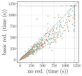
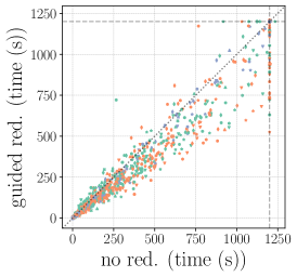
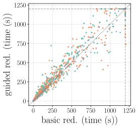
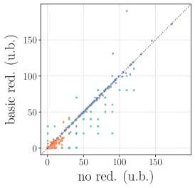
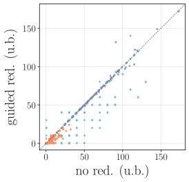
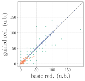
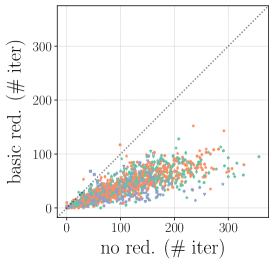
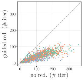
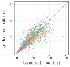
Figure 2: Results on OMT-encoded optimal temporal planning problems.

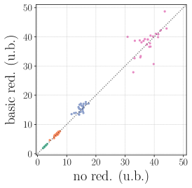
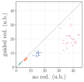
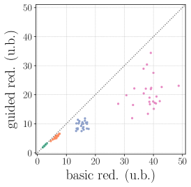
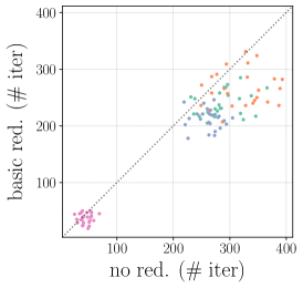
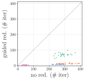
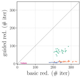
Figure 3: Results on OMT-encoded strip-packing problems.

Figures˜2 and 3 show the results on temporal planning and strip-packing benchmarks, respectively. For each benchmark set, we report a set of scatter plots.

On the rows, we have different metrics, namely the solving time in seconds (time(s)), the upper bound (u.b.) —i.e., the optimum value when the solver terminated within the time limit, or the value of the best solution found within the timeout otherwise— and the number of iterations (# iter) taken to reach the upper bound (see Algorithm˜2).

On the columns, we compare the results obtained with the different truth-assignment-reduction strategies: in the left and center columns, we respectively compare the basic and the guided reductions with the plain algorithm without reductions. In the right column, we compare the two reduction strategies.

Optimal Temporal Planning (Figure˜2).

In these benchmarks, with no truth-assignment reduction, OptiMathSAT reported 246 timeouts, 211 with the basic reduction, and 212 with the guided reduction.

From the plots (first row, left and center columns), we can see that applying either reduction almost uniformly improves the solving time with few exceptions, making optimal solving up to twice as fast as with no reduction.

Moreover, we observe that reducing truth assignments is very effective also for anytime solving (second row, left and center columns). Notice that when the solver terminated within the timeout with both strategies, then the corresponding points lie on the bisector, whereas when at least one strategy times out, the points are generally below the bisector. Indeed, this shows that, for anytime solving, both the basic and the guided reductions allow finding a much better upper bound than with no reduction.

Finally, we can see that both strategies are particularly effective in reducing the number of iterations needed to either find the optimum or to reach the best upper bound within the timeout (third row, left and center). Reducing the number of iterations is not an advantage in itself, but it is a good indicator of the effectiveness of truth-assignment reduction strategies in OMT.

Overall, in these benchmarks there is no clear winner between the two reduction strategies (right column), but it is evident that applying either form of truth-assignment reduction can be beneficial in OMT, both for optimal and anytime solving.

Strip-packing (Figure˜3).

Since no instance in this set of benchmarks terminated within the timeout, for these benchmarks we omit the time plots. We can see that here the basic reduction strategy is not really effective, since the value of the upper bound is not improved compared to the no-reduction strategy (first row, left column). Also, the number of iterations only slightly decreases (second row, left column), suggesting that here blindly removing atoms from the truth assignment does not help much in finding better solutions. On the other hand, the guided reduction strategy is much more effective, since it allows finding a much better upper bound within the timeout (first row, center and right columns), and the number of iterations is drastically reduced (second row, center and right columns).

Discussion.

The results show that applying either form of truth-assignment reduction can be beneficial in OMT, both for optimal and anytime solving. Also, accurately selecting which atoms to remove from the truth assignment can make a significant difference in finding better solutions in fewer iterations. However, we can observe that a much smaller number of iterations, i.e. of truth assignments enumerated, does not always correlate linearly with the solving time. This can be due to several reasons.

First, we notice that in these problems the number of truth assignments enumerated is typically contained, up to a few hundred. In fact, in OMT the bounds on the objective function already allow performing a very effective pruning of the search space.

Moreover, this pruning is typically done by theory reasoning, and most of it has to be done anyway, regardless of the number of truth assignments enumerated. Making it in a single iteration or in many iterations may not reflect as much on the solving time, because of the efficient incrementality of SMT solvers, which can reduce a lot the cost of consecutive iterations. Nevertheless, this suggests that exploiting partial truth assignments in OMT problems with theories where incrementality is not as effective as in $\mathcal{LRA}$, as is the case, e.g., of $\mathcal{LIA}$, can have a larger impact also on the solving time.

6 Conclusions and Future Work

In this paper, we have investigated the role of truth assignment enumeration in OMT solving, and proposed some ways for exploiting partial truth assignments for improving the efficiency and effectiveness of the search. In particular, we have proposed a truth assignment reduction strategy that takes advantage of the properties of the optimization problem to accurately choose the atoms to remove from the truth assignment.

We have implemented the proposed strategies in the OptiMathSAT solver, and evaluated them on a set of $\text{OMT}(\mathcal{LRA})$ benchmarks. Our experimental results show that the proposed strategies can significantly improve the performance of the solver, uniformly reducing the overall solving time for optimal solving, and finding much better solutions for anytime solving.

The results also show that the proposed strategies are particularly effective in reducing the number of search iterations needed to find the optimum solution. This makes it very promising for their applicability in OMT problems where the incrementality of SMT calls is poorly effective, such as in the case of $\mathcal{LIA}$.

In future work, we plan to investigate similar truth-assignment reduction techniques for other SMT theories, in particular $\mathcal{LIA}$.

References

- [1] Albert, E., Correas, J., Gordillo, P., Román-Díez, G., Rubio, A.: GASOL: Gas Analysis and Optimization for Ethereum Smart Contracts. In: TACAS 2020. pp. 118–125. Springer (2020)
- [2] Barrett, C., Sebastiani, R., Seshia, S.A., Tinelli, C.: Satisfiability Modulo Theories. In: Handbook of Satisfiability, FAIA, vol. 336, pp. 1267–1329. IOS Press, 2 edn. (2021)
- [3] Bian, Z., Chudak, F., Macready, W., Roy, A., Sebastiani, R., Varotti, S.: Solving SAT (and MaxSAT) with a quantum annealer: Foundations, encodings, and preliminary results. Inf Comput 275, 104609 (2020)
- [4] Bigarella, F., Cimatti, A., Griggio, A., Irfan, A., Jonáš, M., Roveri, M., Sebastiani, R., Trentin, P.: Optimization Modulo Non-linear Arithmetic via Incremental Linearization. In: FROCOS 2021. pp. 213–231. LNCS, Springer (2021)
- [5] Bjørner, N., Phan, A.D., Fleckenstein, L.: Z - An Optimizing SMT Solver. In: TACAS 2015. pp. 194–199. LNCS, Springer (2015)
- [6] Bofill, M., Coll, J., Suy, J., Villaret, M.: An Efficient SMT Approach to Solve MRCPSP/max Instances with Tight Constraints on Resources. In: CP 2017. pp. 71–79. LNCS, Springer (2017)
- [7] Bozzano, M., Bruttomesso, R., Cimatti, A., Junttila, T., Ranise, S., van Rossum, P., Sebastiani, R.: Efficient Theory Combination via Boolean Search. Inf Comput 204(10), 1493–1525 (2006)
- [8] Cimatti, A., Griggio, A., Schaafsma, B.J., Sebastiani, R.: The MathSAT5 SMT Solver. In: TACAS 2013. pp. 93–107. LNCS, Springer (2013)
- [9] Ding, J., Spallitta, G., Sebastiani, R.: Effective prime factorization via quantum annealing by modular locally-structured embedding. Sci Rep 14(1), 3518 (2024)
- [10] Dutertre, B., de Moura, L.: A Fast Linear-Arithmetic Solver for DPLL(T). In: CAV 2006. pp. 81–94. LNCS, Springer (2006)
- [11] Fried, D., Nadel, A., Sebastiani, R., Shalmon, Y.: Entailing Generalization Boosts Enumeration. In: SAT 2024. LIPIcs, vol. 305, pp. 13:1–13:14. LZI (2024)
- [12] Fried, D., Nadel, A., Shalmon, Y.: AllSAT for Combinational Circuits. In: SAT 2023. LIPIcs, vol. 271, pp. 9:1–9:18. LZI (2023)
- [13] Henry, J., Asavoae, M., Monniaux, D., Maïza, C.: How to compute worst-case execution time by optimization modulo theory and a clever encoding of program semantics. In: LCTES 2014. pp. 43–52. ACM (2014)
- [14] Lahiri, S.K., Nieuwenhuis, R., Oliveras, A.: SMT Techniques for Fast Predicate Abstraction. In: CAV 2006. pp. 424–437. LNCS, Springer (2006)
- [15] Leofante, F., Giunchiglia, E., Ábrahám, E., Tacchella, A.: Optimal Planning Modulo Theories. In: IJCAI 2020. pp. 4128–4134 (2021)
- [16] Li, Y., Albarghouthi, A., Kincaid, Z., Gurfinkel, A., Chechik, M.: Symbolic optimization with SMT solvers. In: POPL 2014. pp. 607–618. ACM (2014)
- [17] Marques-Silva, J., Lynce, I., Malik, S.: Conflict-Driven Clause Learning SAT Solvers. In: Handbook of Satisfiability, FAIA, vol. 336. IOS Press (2021)
- [18] Masina, G., Spallitta, G., Sebastiani, R.: On CNF Conversion for Disjoint SAT Enumeration. In: SAT 2023. LIPIcs, vol. 271, pp. 15:1–15:16. LZI (2023)
- [19] Morgado, A., Marques-Silva, J.: Good Learning and Implicit Model Enumeration. In: ICTAI 2005. pp. 131–136. IEEE Computer Society (2005)
- [20] Nadel, A., Ryvchin, V.: Bit-Vector Optimization. In: TACAS 2016. pp. 851–867. LNCS, Springer (2016)
- [21] Nguyen, C.M., Sebastiani, R., Giorgini, P., Mylopoulos, J.: Multi-objective reasoning with constrained goal models. Requir Eng 23(2), 189–225 (2018)
- [22] Nieuwenhuis, R., Oliveras, A.: On SAT Modulo Theories and Optimization Problems. In: SAT 2006. pp. 156–169. LNCS, Springer (2006)
- [23] Panjkovic, S., Micheli, A.: Expressive Optimal Temporal Planning via Optimization Modulo Theory. AAAI 2023 37(10), 12095–12102 (2023)
- [24] Panjkovic, S., Micheli, A.: Abstract Action Scheduling for Optimal Temporal Planning via OMT. AAAI 2024 38(18), 20222–20229 (2024)
- [25] Plaisted, D.A., Greenbaum, S.: A Structure-preserving Clause Form Translation. J Symb Comput 2(3), 293–304 (1986)
- [26] Ravi, K., Somenzi, F.: Minimal Assignments for Bounded Model Checking. In: TACAS 2004. LNCS, vol. 2988, pp. 31–45. Springer (2004)
- [27] Sebastiani, R.: Lazy Satisfiability Modulo Theories. JSAT 3(3-4), 141–224 (2007)
- [28] Sebastiani, R., Tomasi, S.: Optimization in SMT with LA(Q) Cost Functions. In: IJCAR 2012. LNCS, vol. 7364, pp. 484–498. Springer (2012)
- [29] Sebastiani, R., Tomasi, S.: Optimization Modulo Theories with Linear Rational Costs. ACM Trans. Comput. Logic 16(2), 12:1–12:43 (2015)
- [30] Sebastiani, R., Trentin, P.: Pushing the Envelope of Optimization Modulo Theories with Linear-Arithmetic Cost Functions. In: TACAS 2015. pp. 335–349. LNCS, Springer (2015)
- [31] Sebastiani, R., Trentin, P.: OptiMathSAT: A Tool for Optimization Modulo Theories. J Autom Reason 64(3), 423–460 (2020)
- [32] Spallitta, G., Masina, G., Morettin, P., Passerini, A., Sebastiani, R.: Enhancing SMT-based Weighted Model Integration by Structure Awareness. Artif Intell 328, 104067 (2024)
- [33] Spallitta, G., Sebastiani, R., Biere, A.: Disjoint Partial Enumeration without Blocking Clauses. In: AAAI 2024. vol. 38, pp. 8126–8135 (2024)
- [34] Teso, S., Sebastiani, R., Passerini, A.: Structured learning modulo theories. Artif Intell 244, 166–187 (2017)
- [35] Toda, T., Soh, T.: Implementing Efficient All Solutions SAT Solvers. ACM J. Exp. Algorithmics 21, 1–44 (2016)
- [36] Trentin, P., Sebastiani, R.: Optimization Modulo the Theories of Signed Bit-Vectors and Floating-Point Numbers. J Autom Reason 65(7), 1071–1096 (2021)
- [37] Tseitin, G.S.: On the Complexity of Derivation in Propositional Calculus. In: Automation of Reasoning: 2: Classical Papers on Computational Logic 1967–1970, pp. 466–483. Symbolic Computation, Springer (1983)
- [38] Tsiskaridze, N., Barrett, C., Tinelli, C.: Generalized Optimization Modulo Theories. In: Automated Reasoning. pp. 458–479. Springer (2024)