Numerical analysis of a finite volume method for a $\displaystyle 1$-d wave equation with non smooth wave speed and localized Kelvin-Voigt damping

Abstract.

In this paper, we study the numerical solution of an elastic/viscoelastic wave equation with non smooth wave speed and internal localized distributed Kelvin-Voigt damping acting faraway from the boundary. Our method is based on the Finite Volume Method (FVM) and we are interested in deriving the stability estimates and the convergence of the numerical solution to the continuous one. Numerical experiments are performed to confirm the theoretical study on the decay rate of the solution to the null one when a localized damping acts.

1. Introduction

Numerical simulation is a computation that implements a mathematical model for a physical system. It is required to study the behavior of systems representing complicated mathematical models in order to provide good approximations to the analytical solutions. Numerical modeling uses mathematical models to describe the physical conditions necessary especially for engineers. Still, some of their equations, mostly partial differential equations, are somehow impossible to solve directly. With numerical models, the approximate solutions can be obtained; for example, by Finite Difference Method (FDM), Finite Element Method (FEM) or Finite Volume Method (FVM), with each method having its own merits and limitations. Nevertheless, several results are interpreted within the framework of an engineering process concerning the numerical experiments carried out in these models. However, as mathematicians, numerical studies help us not only in confirming the theoretical results, but also in predicting the solutions of some conjectures. In fact, there are many numerical studies in the literature related to FDM, FEM and FVM. For example, Larsson et al. applied FEM on a strongly damped wave equation (see [12]). In [20], Zuazua et al. considered a problem that models the damped vibrations of a string with fixed ends. Assuming that the damping is localized on a subinterval, FDM with artificial viscosity was applied to show the exponential decay of the discrete energy and to obtain the convergence of the scheme. However, the error estimates were obtained later on by Rincon et al. after applying a spatial FEM (see [17]). Moreover, Gao et al., in [7], presented an unconditionally stable finite difference scheme to find the solution of a one-dimensional linear hyperbolic equation with global damping. Also, Wang et al. used high order FDM to solve the wave equation in the second order form in two space dimensions (see [21]). Furthermore, Xu et al., in [23], considered the Euler-Bernoulli beam equation with local Kelvin-Voigt damping acting via nonsmooth coefficient. Using FEM followed by the control parameterization method, they aim to design a control input numerically distributed locally on a subinterval such that the total energy of the beam and the control on a given time period is minimal. As to FVM, which is based on an integral formulation, it is very popular in solving linear hyperbolic equations. For instance, LeVeque, in [13], used FVM for hyperbolic equations. Also, considering that wave equations are important hyperbolic equations that arise in acoustics, numerical studies were carried on wave-based modeling of room acoustics using FDM and FVM (see [11]). In addition, in [19], explicit numerical simulation has been developed for time dependent viscoelastic flow problems using a combination between FVM and FEM. Zhang et al., in [24], illustrated a new spectral FVM for a $\displaystyle 2$-d and $\displaystyle 3$-d elastic wave equations with external sources on unstructured meshes. Zhang et al. also presented a new efficient FVM for $\displaystyle 3$-d elastic wave simulation on unstructured tetrahedral meshes (see [25]). We aslo mention Riečanová et al. [16], were the authors obtained the stability estimates and convergence of the numerical scheme of a wave equation with Dirichlet boundary condition on a rectangular domain. Their method was based on FVM in space together with the average of $\displaystyle n+1$ and $\displaystyle n-1$ time step diffusion. However, in the one-dimensional case, some authors ensured the decay of energy and gave examples that verify its asymptotic behavior by implementing numerical schemes (see [2, 1, 15, 14]). Thus, to our knowledge, it seems that there are no results in the literature on the convergence and stability estimates, concerning the transmission problem of elastic/viscoelastic systems where there is a discontinuity at the interface, based especially on FVM.

The main objective of this research work is to fill this gap. More precisely, we study the numerical solution of the transmission problem of a wave equation with localized Kelvin-Voigt damping acting faraway from the boundary via nonsmooth coefficient as described in figure 1

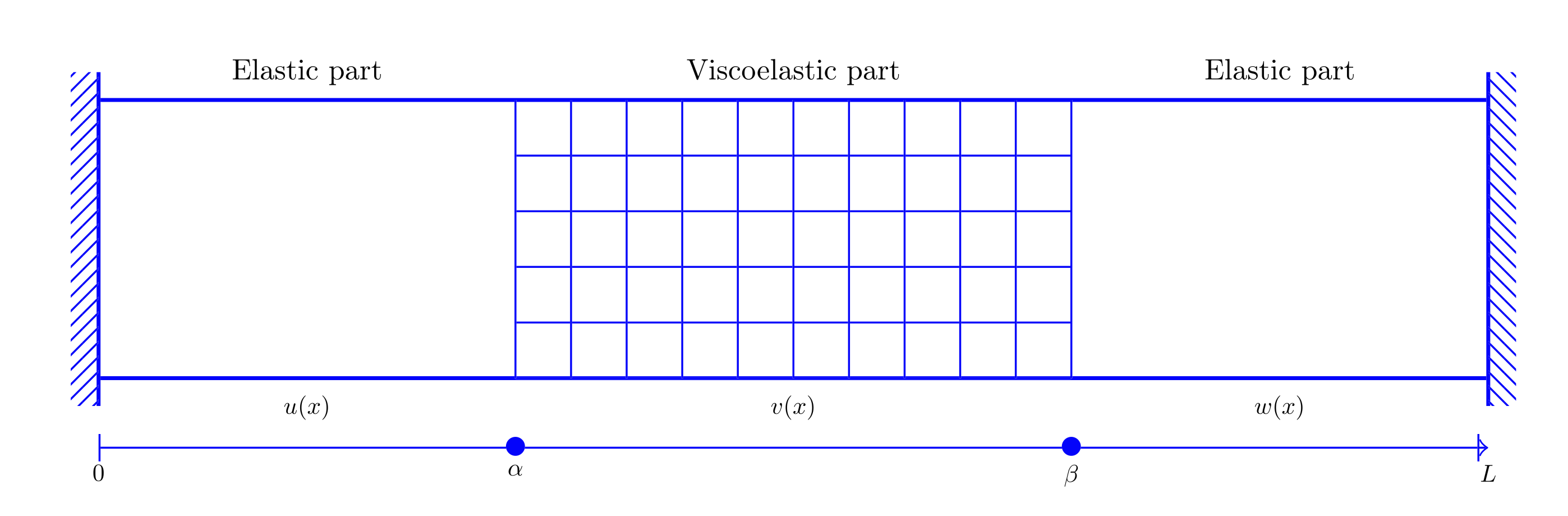
Figure 1. Partial viscoelastic material

Consider the following transmission problem of a wave equation with localized Kelvin-Voigt type damping

(1.1) $$\displaystyle\rho_{1}u_{tt}-\kappa_{1}u_{xx}=0, \displaystyle(x,t)\in(0,\alpha)\times(0,+\infty),$$

(1.2) $$\displaystyle\rho_{2}v_{tt}-\kappa_{2}v_{xx}-\varrho v_{xxt}=0, \displaystyle(x,t)\in(\alpha,\beta)\times(0,+\infty),$$

(1.3) $$\displaystyle\rho_{3}w_{tt}-\kappa_{3}w_{xx}=0, \displaystyle(x,t)\in(\beta,L)\times(0,+\infty).$$

Here $\displaystyle\rho_{1},\ \rho_{2},\ \rho_{3},\kappa_{1},\ \kappa_{2}$ and $\displaystyle\kappa_{3}$ are strictly positive constant numbers representing the density and metric coefficients of Equations (1.1), (1.2) and (1.3) respectively and the damping constant $\displaystyle\varrho$ is strictly positive. In fact, we divide Equations (1.1)-(1.3) by $\displaystyle\rho_{1},\ \rho_{2}$ and $\displaystyle\rho_{3}$ respectively to obtain

(1.4) $$\displaystyle u_{tt}-C_{1}^{2}u_{xx}=0, \displaystyle(x,t)\in(0,\alpha)\times(0,+\infty),$$

(1.5) $$\displaystyle v_{tt}-C_{2}^{2}v_{xx}-\delta v_{xxt}=0, \displaystyle(x,t)\in(\alpha,\beta)\times(0,+\infty),$$

(1.6) $$\displaystyle w_{tt}-C_{3}^{2}w_{xx}=0, \displaystyle(x,t)\in(\beta,L)\times(0,+\infty).$$

System (1.4)-(1.6) is subjected to the Dirichlet boundary conditions

(1.7) $$u(0,t)=w(L,t)=0,\quad t\in(0,+\infty)$$

and the following initial conditions

(1.8) $$\left\{\begin{array}[]{ll}u(x,0)=\varphi(x),&x\in(0,\alpha),\\ v(x,0)=\eta(x),&x\in(\alpha,\beta),\\ w(x,0)=\gamma(x),&x\in(\beta,L)\ ,\end{array}\right.$$

(1.9) $$\left\{\begin{array}[]{ll}u_{t}(x,0)=\psi(x),&x\in(0,\alpha),\\ v_{t}(x,0)=\zeta(x),&x\in(\alpha,\beta),\\ w_{t}(x,0)=\theta(x),&x\in(\beta,L)\ .\end{array}\right.$$

We set $\displaystyle\Phi=(\varphi,\eta,\gamma)$ and $\displaystyle\Psi=(\psi,\zeta,\theta)$; $\displaystyle C_{1}=\sqrt{\frac{\kappa_{1}}{\rho_{1}}}$, $\displaystyle C_{2}=\sqrt{\frac{\kappa_{2}}{\rho_{2}}}$ and $\displaystyle C_{3}=\sqrt{\frac{\kappa_{3}}{\rho_{3}}}$ represent the speed of the wave propagation of Equations (1.4)-(1.6) respectively. Also, $\displaystyle\delta=\frac{\varrho}{\rho_{2}}$.

The transmission conditions are given by

(1.10) $$\left\{\begin{array}[]{ll}\displaystyle{\par u(\alpha,t)=v(\alpha,t),\quad v(\beta,t)=w(\beta,t)},&t\in(0,+\infty),\\ \displaystyle{C_{2}^{2}v_{x}(\alpha,t)+\delta v_{xt}(\alpha,t)=C_{1}^{2}u_{x}(\alpha,t)},&t\in(0,+\infty),\\ \displaystyle{C_{2}^{2}v_{x}(\beta,t)+\delta v_{xt}(\beta,t)=C_{3}^{2}w_{x}(\beta,t),}&t\in(0,+\infty).\end{array}\right.$$

Definition 1 (Weak solution).

Let us define the functional spaces:

$$\begin{array}[]{ll}\displaystyle{\mathbb{H}^{1}=H^{1}(0,\alpha)\times H^{1}(\alpha,\beta)\times H^{1}(\beta,L),}\\ \displaystyle{\mathbb{L}^{2}=L^{2}(0,\alpha)\times L^{2}(\alpha,\beta)\times L^{2}(\beta,L)},\\ \displaystyle{\mathbb{H}^{1}_{L}=\{(u,v,w)\in\mathbb{H}^{1}\ |\ u(0)=w(L)=0,\ u(\alpha)=v(\alpha),\ v(\beta)=w(\beta)\}.}\end{array}$$

We say that $\displaystyle U=(u,v,w)$ is a weak solution of the System (1.4)-(1.10) if for all $\displaystyle T>0$, the following conditions hold:

• $\displaystyle U=(u,v,w)\in L^{2}([0,T];\mathbb{H}^{1}_{L})$ and $\displaystyle U_{t}=(u_{t},v_{t},w_{t})\in L^{2}([0,T];\mathbb{L}^{2})$,

• $\displaystyle(u(.,0),v(.,0),w(.,0))=(\varphi(.),\eta(.),\gamma(.))$,

• (1.11) $$\begin{array}[]{lll}-\int_{0}^{T}\int_{0}^{\alpha}u_{t}p_{t}dxdt+C_{1}^{2}\int_{0}^{T}\int_{0}^{\alpha}u_{x}p_{x}dxdt-\int_{0}^{\alpha}\psi(x)p(x,0)dx\\ -\int_{0}^{T}\int_{\alpha}^{\beta}v_{t}q_{t}dxdt+C_{2}^{2}\int_{0}^{T}\int_{\alpha}^{\beta}v_{x}q_{x}dxdt+\delta\int_{0}^{T}\int_{\alpha}^{\beta}v_{tx}q_{x}dxdt-\int_{\alpha}^{\beta}\zeta(x)q(x,0)dx\\ -\int_{0}^{T}\int_{\beta}^{L}w_{t}z_{t}dxdt+C_{3}^{2}\int_{0}^{T}\int_{\beta}^{L}w_{x}z_{x}dxdt-\int_{\beta}^{L}\theta(x)z(x,0)dx=0\end{array}$$

  for all $\displaystyle(p,q,z)\in L^{2}([0,T];\mathbb{H}^{1}_{L})$ and $\displaystyle(p_{t},q_{t},z_{t})\in L^{2}([0,T];\mathbb{L}^{2})$ such that

  $$p(T,x)=0\,,\,q(T,x)=0\mbox{ and }z(T,x)=0\quad.$$

We study our problem under the following hypothesis $\displaystyle\eqref{H'}$:

(H^′) $$\Phi\in\mathbb{H}^{1}_{L},\quad\Psi\in\mathbb{H}^{1}.$$

The energy of the solutions of the System (1.4)-(1.10) is defined by

(1.12) $$E(t)=\dfrac{1}{2}\int_{0}^{\alpha}|{u_{t}}|^{2}+\dfrac{C_{1}^{2}}{2}\int_{0}^{\alpha}|{u_{x}}|^{2}+\dfrac{1}{2}\int_{\alpha}^{\beta}|{v_{t}}|^{2}+\dfrac{C_{2}^{2}}{2}\int_{\alpha}^{\beta}|{v_{x}}|^{2}+\dfrac{1}{2}\int_{\beta}^{L}|{w_{t}}|^{2}+\dfrac{C_{3}^{2}}{2}\int_{\beta}^{L}|{w_{x}}|^{2}$$

Let $\displaystyle U=(u,v,w)\in L^{2}([0,T];\mathbb{H}^{1}_{L})$ and $\displaystyle U_{t}=(u_{t},v_{t},w_{t})\in L^{2}([0,T];\mathbb{L}^{2})$ be a weak solution of the system (1.4)-(1.10). Then we have the following dissipativity estimation:

(1.13) $$\forall t>0\,,\,\dfrac{dE(t)}{dt}=-\delta\int_{\alpha}^{\beta}|{v_{x}t}|^{2}$$

The theoretical study of such systems was done in previous literature (see [9, 22, 8, 3, 18, 4]). In [9], the authors studied the asymptotic behavior of the energy of the continuous case of system (1.4)-(1.10) and obtained an optimal energy decay rate of type $\displaystyle t^{-4}$. In this article, our objective is to study this system numerically. To this aim, in Section 2, we discretize our system using an admissible mesh and set the explicit numerical scheme in Subsection 2.2 and the semi-implicit numerical scheme with an average of $\displaystyle n+1$ and $\displaystyle n-1$ time step diffusion in Subsection 2.4 using FVM in space. However, in Subsections 2.3 and 2.5, we design a discrete energy that dissipates when the control is acting and is conserved during its absence. Sections 3 and 4 are devoted to stability estimates and convergence of the discrete solution to the continuous one. Finally, in Section 5, we give some numerical examples which demonstrate the theoretical results obtained in [9].
We also mention that in [9] two of the authors have proved the existence and uniqueness of a strong solution $\displaystyle U=(u,v,w)\in L^{2}([0,T];\mathbb{H}^{1}_{L})$ and $\displaystyle U_{t}=(u_{t},v_{t},w_{t})\in L^{2}([0,T];\mathbb{L}^{2})$. So the existence and uniqueness of the weak solution is thus verified.

2. Construction of the discretization of the problem

In this section, we will firstly define the admissible mesh and the discrete unknowns according to the Finite Volume Method.

Then we will construct an explicit in time Finite Volume discretization. We will build a discrete energy and will prove that this discrete energy is decreasing in time.

Finally we will construct an implicit in time Finite Volume discretization. Again, we will build a discrete energy and will prove that this discrete energy is decreasing in time.

2.1. Admissible one-dimensional mesh and defintition of the discrete unknowns

An admissible mesh $\displaystyle\mathcal{T}$ of the interval $\displaystyle(0,L)$ is given by a family $\displaystyle\{K_{i}:\ i\in\{1,\cdots,N_{\max}\};\leavevmode\nobreak\ \ N_{\max}\in\mathbb{N}^{*}\}$ of control volumes such that $\displaystyle K_{i}=(x_{i-\frac{1}{2}},x_{i+\frac{1}{2}})$ and a family $\displaystyle(x_{i})_{i=0,\cdots,N_{\max}+1}$ assumed to be the center of $\displaystyle(K_{i})_{i=1,\cdots,N_{\max}}$ such that

$$0=x_{0}=x_{\frac{1}{2}}<x_{1}<x_{\frac{3}{2}}<x_{2}<\cdots<x_{i-\frac{1}{2}}<x_{i}<x_{i+\frac{1}{2}}<\cdots<x_{N_{\rm{max}}}<x_{N_{\rm{max}}+\frac{1}{2}}=x_{N_{\rm{max}}+1}=L.$$

We discretize the intervals $\displaystyle[0,\alpha]$, $\displaystyle[\alpha,\beta]$ and $\displaystyle[\beta,L]$ into $\displaystyle N_{\alpha}$, $\displaystyle N$ and $\displaystyle N_{\beta}$ internal points respectively such that $\displaystyle N_{\alpha},N,N_{\beta}\in\mathbb{N}^{*}$ and $\displaystyle N_{\max}=N_{\alpha}+N+N_{\beta}$. To be clear, let $\displaystyle h_{\alpha}=\alpha/N_{\alpha},\ h=(\beta-\alpha)/N$ and $\displaystyle h_{\beta}=(L-\beta)/N_{\beta}$ and discretize as the following:
We discretize $\displaystyle[0,\alpha]$ such that:

• For $\displaystyle i=0,\ldots,N_{\alpha}$, $\displaystyle x_{i+\frac{1}{2}}=ih_{\alpha},$ which yields, $\displaystyle x_{\frac{1}{2}}=0$ and $\displaystyle x_{N_{\alpha}+\frac{1}{2}}=\alpha.$

• For $\displaystyle i=1,\ldots,N_{\alpha}$, $\displaystyle x_{i}=\bigg{(}i-\frac{1}{2}\bigg{)}h_{\alpha}$, which yields, $\displaystyle x_{1}=\frac{h_{\alpha}}{2}$ and $\displaystyle x_{N_{\alpha}}=\alpha-\frac{h_{\alpha}}{2}$.

We discretize $\displaystyle[\alpha,\beta]$ such that:

• For $\displaystyle i=N_{\alpha}+1,\ldots,N_{\alpha}+N$, $\displaystyle x_{i+\frac{1}{2}}=\alpha+(i-N_{\alpha})h,$ which yields, $\displaystyle x_{N_{\alpha}+\frac{3}{2}}=\alpha+h$ and $\displaystyle x_{N_{\alpha}+N+\frac{1}{2}}=\beta$.

• For $\displaystyle i=N_{\alpha}+1,\ldots,N_{\alpha}+N$, $\displaystyle x_{i}=\alpha+\bigg{(}i-N_{\alpha}-\frac{1}{2}\bigg{)}h$, which yields, $\displaystyle x_{N_{\alpha}+1}=\alpha+\frac{h}{2}$ and $\displaystyle x_{N_{\alpha}+N}=\beta-\frac{h}{2}$.

We discretize $\displaystyle[\beta,L]$ such that:

• For $\displaystyle i=N_{\alpha}+N+1,\ldots,N_{\max}$, $\displaystyle x_{i+\frac{1}{2}}=\beta+(i-N_{\alpha}-N)h_{\beta},$ which yields, $\displaystyle x_{N_{\alpha}+N+\frac{3}{2}}=\beta+h_{\beta}$ and $\displaystyle x_{N_{\max}+\frac{1}{2}}=L$.

• For $\displaystyle i=N_{\alpha}+N+1,\ldots,N_{\max}$, $\displaystyle x_{i}=\beta+\bigg{(}i-N_{\alpha}-N-\frac{1}{2}\bigg{)}h_{\beta}$, which yields, $\displaystyle x_{N_{\alpha}+N+1}=\beta+\frac{h_{\beta}}{2}$ and $\displaystyle x_{N_{\max}}=L-\frac{h_{\beta}}{2}$.

Now, we set

• $\displaystyle h_{i}=x_{i+\frac{1}{2}}-x_{i-\frac{1}{2}};\ i=1,\ldots,N_{\max},$

• $\displaystyle h_{i+\frac{1}{2}}=x_{i+1}-x_{i};\ i=0,\ldots,N_{\max}$,

• $\displaystyle h_{i-\frac{1}{2}}=x_{i}-x_{i-1};\ i=1,\ldots,N_{\max}+1$,

• $\displaystyle h_{i}^{+}=x_{i+\frac{1}{2}}-x_{i};\ i=1,\ldots,N_{\max}$,

• $\displaystyle h_{i}^{-}=x_{i}-x_{i-\frac{1}{2}};\ i=1,\ldots,N_{\max}$,

• size$\displaystyle(\mathcal{T})=\max\{h_{i},\ i=1,\ldots,N_{\max}\}$.

Figure 2. A model representing the admissible one-dimensional mesh

The interval $\displaystyle(0,L)$ is discretized using the admissible mesh provided above.

The time discretization is performed with a constant time step $\displaystyle\Delta t=\frac{T}{\mathcal{N}}$ with $\displaystyle t_{n+1}-t_{n}=\Delta t$ for all $\displaystyle n=0,1,\cdots,\mathcal{N}$ so that for a function $\displaystyle v$ defined on $\displaystyle[0,L]\times[0,T]$, $\displaystyle v^{n}$ represents the value of the function at time $\displaystyle t_{n}$

We denote the first and second discrete time derivatives following a backward difference and a second-order central difference at time $\displaystyle t_{n}$ as:

$$\partial^{1}v^{n}=\frac{v^{n}-v^{n-1}}{\Delta t}\quad\textrm{and}\quad\partial^{2}v^{n}=\frac{v^{n+1}-2v^{n}+v^{n-1}}{\Delta t^{2}}\,,\,$$

and the centered time discretization is denoted by:

(2.1) $$\partial^{1/2}v^{n}=\frac{v^{n+1}-v^{n-1}}{2\Delta t}\ .$$

Now, for the time step $\displaystyle\Delta t$, we set the following condition

(TA) $$\textrm{There exists}\ \tau_{0}\in[0,T]\ \textrm{such that}\ \Delta t\leq\tau_{0}.$$

We designate the discrete unknowns by $\displaystyle\{u_{i}^{n};\leavevmode\nobreak\ \ i=1,\cdots,N_{\alpha},\leavevmode\nobreak\ \ n\in\mathbb{N}\}$, $\displaystyle\{v_{i}^{n};\leavevmode\nobreak\ \ i=N_{\alpha}+1,\cdots,N_{\alpha}+N,\leavevmode\nobreak\ \ n\in\mathbb{N}\}$, $\displaystyle\{w_{i}^{n};\leavevmode\nobreak\ \ i=N_{\alpha}+N+1,\cdots,N_{\max},\leavevmode\nobreak\ \ n\in\mathbb{N}\}$ where they stand for approximation of the mean values of $\displaystyle u,\ v,\ w$ over the control volumes $\displaystyle K_{i}$ respectively at time $\displaystyle t_{n}$ defined by:

(2.2) $$\displaystyle u_{i}(t) \displaystyle= \displaystyle\frac{1}{h_{i}}\int_{x_{i}-\frac{1}{2}}^{x_{i}+\frac{1}{2}}u(x,t)dx,\quad i=1,\ldots,N_{\alpha}\,,\,t\in[0,T]$$

(2.3) $$\displaystyle v_{i}(t) \displaystyle= \displaystyle\frac{1}{h_{i}}\int_{x_{i}-\frac{1}{2}}^{x_{i}+\frac{1}{2}}v(x,t)dx,\quad i=N_{\alpha}+1,\ldots,N_{\alpha}+N\,,\,t\in[0,T]$$

(2.4) $$\displaystyle w_{i}(t) \displaystyle= \displaystyle\frac{1}{h_{i}}\int_{x_{i}-\frac{1}{2}}^{x_{i}+\frac{1}{2}}w(x,t)dx,\quad i=N_{\alpha}+N+1,\ldots,N_{\max}\,,\,t\in[0,T]$$

$$\displaystyle u_{i}^{n} \displaystyle= \displaystyle u_{i}(t_{n})\quad i=1,\ldots,N_{\alpha},$$

$$\displaystyle v_{i}^{n} \displaystyle= \displaystyle v_{i}(t_{n})\quad i=N_{\alpha}+1,\ldots,N_{\alpha}+N,$$

$$\displaystyle w_{i}^{n} \displaystyle= \displaystyle w_{i}(t_{n})\quad i=N_{\alpha}+N+1,\ldots,N_{\max}.$$

We next define :

$$\displaystyle U_{i}^{n}=\left\{\begin{array}[]{lllll}u_{i}^{n},&i=1,\ldots,N_{\alpha},\\ v_{i}^{n},&i=N_{\alpha}+1,\ldots,N_{\alpha}+N,\\ w_{i}^{n},&i=N_{\alpha}+N+1,\ldots,N_{\max}.\end{array}\right.\;.$$

It is completed by the Dirichlet boundary conditions : $\displaystyle u_{0}^{n}=U_{0}^{n}=0\,,\,w_{N_{\max}+1}^{n}=U_{N_{\max}+1}^{n}=0$.

The reconstructed solution is defined by $\displaystyle U_{\mathcal{T},\Delta t}$ constant over the control volumes $\displaystyle K_{i}$ at time $\displaystyle t\in[t_{n},t_{n+1})$ as:

(2.5) $$\textrm{ for }t\in[t_{n},t_{n+1})\,,\,\textrm{ for }x\in K_{i}\,,\,U_{\mathcal{T},\Delta t}(x,t)=U_{i}^{n}$$

For a function of only one space variable, we denote $\displaystyle U_{\mathcal{T}}$ the reconstructed solution constant over the control volumes $\displaystyle K_{i}$:

(2.6) $$\textrm{ for }x\in K_{i}\,,\,U_{\mathcal{T}}(x)=U_{i}$$

The initial solution $\displaystyle U_{\mathcal{T}}^{0}$ is constructed according to the initial condition (1.8):

(2.7) $$\left\{\begin{array}[]{lll}u_{i}^{0}=\varphi_{i}\quad\textrm{where}\leavevmode\nobreak\ \ \varphi_{i}=\frac{1}{h_{i}}\int_{K_{i}}\varphi(x)dx,&\textrm{for}\ i=1,\cdots,N_{\alpha},\\ v_{i}^{0}=\eta_{i}\quad\textrm{where}\leavevmode\nobreak\ \ \eta_{i}=\frac{1}{h_{i}}\int_{K_{i}}\eta(x)dx,&\textrm{for}\ i=N_{\alpha}+1,\cdots,N_{\alpha}+N,\\ w_{i}^{0}=\gamma_{i}\quad\textrm{where}\leavevmode\nobreak\ \ \varphi_{i}=\frac{1}{h_{i}}\int_{K_{i}}\gamma(x)dx,&\textrm{for}\ i=N_{\alpha}+N+1,\cdots,N_{\textrm{max}}\\ \Phi_{i}=(\varphi_{i},\eta_{i},\gamma_{i}).\end{array}\right.$$

We set $\displaystyle\Phi_{\mathcal{T}}=(\Phi_{i})_{i=1,\ldots,Nmax}$ so that the initial solution is defined by:

(2.8) $$U^{0}=\Phi_{\mathcal{T}}$$

In order to discretize the initial condition (1.9), we define a “ghost” time-boundary (i.e. $\displaystyle t_{-1}=-\Delta t$) and we use the second-order central difference formula (2.1) at time $\displaystyle t=0$. Indeed as we have :

$$\dfrac{\partial\displaystyle\int_{K_{i}}U(x,t)dx}{\partial t}=\int_{K_{i}}\dfrac{\partial U(x,t)}{\partial t}dx$$

we define:

$$\displaystyle u_{i}^{-1} \displaystyle i=1,\cdots,N_{\alpha},$$ for

$$\displaystyle v_{i}^{-1} \displaystyle i=N_{\alpha}+1,\cdots,N_{\alpha}+N,$$ for

$$\displaystyle w_{i}^{-1} \displaystyle i=N_{\alpha}+N+1\cdots,N_{\textrm{max}}.$$ for

and we set $\displaystyle\Psi_{i}=(\psi_{i},\zeta_{i},\theta_{i})$ such that :

$$\begin{array}[]{lll}\psi_{i}=\frac{1}{h_{i}}\int_{K_{i}}\psi(x)dx,&\textrm{for}\ i=1,\cdots,N_{\alpha},\\ \zeta_{i}=\frac{1}{h_{i}}\int_{K_{i}}\zeta(x)dx,&\textrm{for}\ i=N_{\alpha}+1,\cdots,N_{\alpha}+N,\\ \theta_{i}=\frac{1}{h_{i}}\int_{K_{i}}\theta(x)dx,&\textrm{for}\ i=N_{\alpha}+N+1,\cdots,N_{\max}.\end{array}$$

Therefore, using the above notations, we can approximate the initial conditions of $\displaystyle u_{t}$, $\displaystyle v_{t}$ and $\displaystyle w_{t}$ using centered time approximation:

$$\Psi(x)=\dfrac{\partial U}{\partial t}(x,0)\simeq\dfrac{U(x,\Delta t)-U(x,-\Delta t)}{2\Delta t}$$

to get

$$\begin{array}[]{lll}u_{i}^{-1}=u_{i}^{1}-2\Delta t\psi_{i},&\textrm{for}\ i=1,\cdots,N_{\alpha},\\ v_{i}^{-1}=v_{i}^{1}-2\Delta t\zeta_{i},&\textrm{for}\ i=N_{\alpha}+1,\cdots,N_{\alpha}+N,\\ w_{i}^{-1}=w_{i}^{1}-2\Delta t\theta_{i},&\textrm{for}\ i=N_{\alpha}+N+1,\cdots,N_{\max}\\ \Psi_{i}=(\psi_{i},\zeta_{i},\theta_{i}).\end{array}$$

Consequently, we set $\displaystyle\Psi_{\mathcal{T}}=(\Psi_{i})_{i=1,\ldots,Nmax}$ so that the solution at the “ghost” time-boundary is defined by:

(2.9) $$U^{-1}=U^{1}-2\Delta t\Psi_{\mathcal{T}}\ .$$

As the speed $\displaystyle C$ is defined by

$$C=\left\{\begin{array}[]{lllll}C_{1},&x\in(0,\alpha),\\ C_{2},&x\in(\alpha,\beta),\\ C_{3},&x\in(\beta,L)\end{array}\right.$$

we define the discrete speeds as:

$$\displaystyle c_{i}=C_{1}\quad \displaystyle\textrm{for}\ i=1,\cdots,N_{\alpha},$$

$$\displaystyle c_{i}=C_{2}\quad \displaystyle\textrm{for}\ i=N_{\alpha}+1,\cdots,N_{\alpha}+N,$$

$$\displaystyle c_{i}=C_{3}\quad \displaystyle\textrm{for}\ i=N_{\alpha}+N+1,\cdots,N_{\max}.$$

Now, we will construct the numerical schemes.

2.2. Construction of the explicit discretized problem.

In this part, we will construct the numerical scheme to find the solution of System (1.4)-(1.10) using the Finite Volume Method (FVM) in space and finite difference method in time. The principle of FVM is to integrate the equations (1.4)-(1.5)-(1.6) over the controle volume $\displaystyle K_{i}$. A flux at the boundaries of the control volume will come up typically $\displaystyle-c_{i}^{2}U_{x}(x_{i+\frac{1}{2}},t_{n})$. Thus a reasonable choice for the approximation of $\displaystyle-c_{i}^{2}U_{x}(x_{i+\frac{1}{2}},t_{n})$ is the differential quotient :

$$F_{i+{\frac{1}{2}}}^{n}=\left\{\begin{array}[]{lllll}-C_{1}^{2}\frac{u_{1}^{n}}{h_{\frac{1}{2}}},&i=0,\\ -c_{i}^{2}\frac{U_{i+1}^{n}-U_{i}^{n}}{h_{i+\frac{1}{2}}},&i=1,\ldots,N_{\max}-1,\\ C_{3}^{2}\frac{w_{N_{\max}}^{n}}{h_{N_{\max}+\frac{1}{2}}},&i=N_{\max}.\end{array}\right.$$

Later in this paper, we will adapt the formula for the fluxes at the inner boundary points $\displaystyle x_{i+\frac{1}{2}}=\alpha\mbox{ and }x_{i+\frac{1}{2}}=\beta$. We denote $\displaystyle\ell_{i+\frac{1}{2}}=\frac{c_{i}^{2}}{h_{i+\frac{1}{2}}}$.

Discretization of Equation (1.4).

In this part, we will detail every computations in order to avoid the redaction of the computations for the next parts.

$\displaystyle\Box$ For $\displaystyle i=1,\cdots,N_{\alpha}-1$.

$$\displaystyle\int_{K_{i}}u_{tt}(x,t_{n})dx-C_{1}^{2}\int_{K_{i}}u_{xx}(x,t_{n})dx \displaystyle=0,$$

$$\displaystyle\int_{x_{i-\frac{1}{2}}}^{x_{i+\frac{1}{2}}}u_{tt}(x,t_{n})dx-C_{1}^{2}\int_{x_{i-\frac{1}{2}}}^{x_{i+\frac{1}{2}}}u_{xx}(x,t_{n})dx \displaystyle=0.$$

Let us again remark that

$$\displaystyle\dfrac{\partial^{2}\displaystyle\int_{K_{i}}U(x,t)dx}{\partial t^{2}} \displaystyle=\int_{K_{i}}\dfrac{\partial^{2}U(x,t)}{\partial t^{2}}dx\mbox{ and }$$

$$\displaystyle\int_{x_{i-\frac{1}{2}}}^{x_{i+\frac{1}{2}}}u_{xx}(x,t_{n})dx \displaystyle=u_{x}(x_{i+\frac{1}{2}},t_{n})-u_{x}(x_{i-\frac{1}{2}},t_{n})\ .$$

So we firstly obtain:

$$\frac{1}{h_{i}}\int_{x_{i-\frac{1}{2}}}^{x_{i+\frac{1}{2}}}u_{tt}(x,t_{n})dx=\frac{1}{h_{i}}\bigg{(}\int_{x_{i-\frac{1}{2}}}^{x_{i+\frac{1}{2}}}u(x,t_{n})dx\bigg{)}_{tt}=[u_{i}(t_{n})]_{tt}.$$

A direct calculation gives

$$\begin{array}[]{lll}h_{i}[u_{i}(t_{n})]_{tt}-C_{1}^{2}[u_{x}(x_{i+\frac{1}{2}},t_{n})-u_{x}(x_{i-\frac{1}{2}},t_{n})]=0.\end{array}$$

Using second-order central time discretization at time $\displaystyle t_{n}$ and the fluxes approximation defined before, we obtain:

$$h_{\alpha}\frac{u_{i}^{n+1}-2u_{i}^{n}+u_{i}^{n-1}}{\Delta t^{2}}-\big{[}\ell_{i+\frac{1}{2}}(u^{n}_{i+1}-u^{n}_{i})-\ell_{i-\frac{1}{2}}(u^{n}_{i}-u^{n}_{i-1})\big{]}=0.$$

$\displaystyle\Box$ For $\displaystyle i=N_{\alpha}$ that is $\displaystyle x_{N_{\alpha}+\frac{1}{2}}=\alpha$.

$$\displaystyle\int_{x_{N_{\alpha}-\frac{1}{2}}}^{x_{N_{\alpha}+\frac{1}{2}}}u_{tt}dx-C_{1}^{2}\int_{x_{N_{\alpha}-\frac{1}{2}}}^{x_{N_{\alpha}+\frac{1}{2}}}u_{xx}dx \displaystyle=0,$$

$$\displaystyle h_{N_{\alpha}}[u_{N_{\alpha}}(t_{n})]_{tt}-C_{1}^{2}[u_{x}(x_{N_{\alpha}+\frac{1}{2}},t_{n})-u_{x}(x_{N_{\alpha}-\frac{1}{2}},t_{n})] \displaystyle=0.$$

Let $\displaystyle H_{i+\frac{1}{2}}$ represent the approximation of the flux $\displaystyle c_{i}^{2}u_{x}(x_{i+\frac{1}{2}},t_{n})$ for $\displaystyle i=N_{\alpha}$. Using the finite difference principle, we have

$$\begin{array}[]{lll}H_{i+\frac{1}{2}}=c_{i}^{2}\frac{u_{i+\frac{1}{2}}^{n}-u_{i}^{n}}{h_{i}^{+}}&\textrm{over}\ K_{i};\ i=N_{\alpha},\\ H_{i+\frac{1}{2}}=c_{i+1}^{2}\frac{{u^{n}_{i+1}}-u^{n}_{{i+\frac{1}{2}}}}{h_{i+1}^{-}}&\textrm{over}\ K_{i+1};\ i=N_{\alpha}.\end{array}$$

where $\displaystyle u_{i+\frac{1}{2}}^{n}$ is unknown and represents an approximation of $\displaystyle u(\alpha,t_{n})$.

Since $\displaystyle x_{i}$ is the center of $\displaystyle K_{i}$ for all $\displaystyle i$, then substituting $\displaystyle i=N_{\alpha}$ gives

$$\begin{array}[]{lll}H_{i+\frac{1}{2}}=c_{i}^{2}\frac{u_{i+\frac{1}{2}}^{n}-u_{i}^{n}}{\frac{h_{\alpha}}{2}}&\textrm{over}\ K_{i};\ i=N_{\alpha},\\ H_{i+\frac{1}{2}}=c_{i+1}^{2}\frac{{u^{n}_{i+1}}-u^{n}_{{i+\frac{1}{2}}}}{\frac{h}{2}}&\textrm{over}\ K_{i+1};\ i=N_{\alpha}\end{array}$$

The above approximations should be equal to guarantee the conservation of the flux (see [5]), and thus we get by a direct calculation

(2.10) $$H_{i+\frac{1}{2}}=\frac{c_{i}^{2}c_{i+1}^{2}}{\frac{h}{2}c^{2}_{i}+\frac{h_{\alpha}}{2}c_{i+1}^{2}}(u_{i+1}^{n}-u_{i}^{n})\quad\textrm{for}\ i=N_{\alpha}.$$

Given that for $\displaystyle i=N_{\alpha}$, $\displaystyle c_{i+1}=C_{2}$ and $\displaystyle c_{i}=C_{1}$, we change the value of $\displaystyle\ell_{N_{\alpha}+\frac{1}{2}}$ as $\displaystyle\ell_{N_{\alpha}+\frac{1}{2}}=\frac{2C_{1}^{2}C_{2}^{2}}{C_{1}^{2}h+C_{2}^{2}h_{\alpha}}$ to obtain :

$$C_{1}^{2}u_{x}(x_{N_{\alpha}+\frac{1}{2}},t_{n})\simeq\ell_{N_{\alpha}+\frac{1}{2}}(v^{n}_{N_{\alpha}+1}-u^{n}_{N_{\alpha}})\ ,$$

taking into consideration that $\displaystyle u_{N_{\alpha}+1}$ is actually $\displaystyle v_{N_{\alpha}+1}$ due to the continuity of the functions at the interface.

Remark 1.

Let us remark that we have :

(2.11) $$\min(C_{1}^{2},C_{2}^{2})\leq\ell_{N_{\alpha}+\frac{1}{2}}\times h_{N_{\alpha}+\frac{1}{2}}\leq\max(C_{1}^{2},C_{2}^{2})\ .$$

We will use these inequalities to obtain an estimation of the discrete $\displaystyle\mathbb{H}^{1}$ semi-norm (see lemma 3.4)

Now, using the second-order central difference in time and forward difference discretization in space, we obtain

$$\displaystyle h_{\alpha}\frac{u_{N_{\alpha}}^{n+1}-2u_{N_{\alpha}}^{n}+u_{N_{\alpha}}^{n-1}}{\Delta t^{2}}-\big{[}\ell_{N_{\alpha}+\frac{1}{2}}(v^{n}_{N_{\alpha}+1}-u^{n}_{N_{\alpha}})-\ell_{N_{\alpha}-\frac{1}{2}}(u^{n}_{N_{\alpha}}-u^{n}_{N_{\alpha}-1})\big{]} \displaystyle=0.$$

Discretization of Equation (1.5).
$\displaystyle\Box$ For $\displaystyle i=N_{\alpha}+1$:

$$\displaystyle\int_{x_{N_{\alpha}+\frac{1}{2}}}^{x_{N_{\alpha}+\frac{3}{2}}}v_{tt}dx-C_{2}^{2}\int_{x_{N_{\alpha}+\frac{1}{2}}}^{x_{N_{\alpha}+\frac{3}{2}}}v_{xx}dx-\delta\int_{x_{N_{\alpha}+\frac{1}{2}}}^{x_{N_{\alpha}+\frac{3}{2}}}v_{xxt}dx \displaystyle=0,$$

$$\displaystyle h_{N_{\alpha}+1}[v_{N_{\alpha}+1}(t)]_{tt}-C_{2}^{2}[v_{x}(x_{N_{\alpha}+\frac{3}{2}},t_{n})-v_{x}(x_{N_{\alpha}+\frac{1}{2}},t_{n})]-\delta[v_{xt}(x_{N_{\alpha}+\frac{3}{2}},t_{n})-v_{xt}(x_{N_{\alpha}+\frac{1}{2}},t_{n})] \displaystyle=0.$$

First of all, since the position $\displaystyle x_{N_{\alpha}+\frac{1}{2}}$ represents the point $\displaystyle\alpha$, then we use the transmission condition (1.10) at point $\displaystyle\alpha$ and thus

$$C_{2}^{2}v_{x}(x_{N_{\alpha}+\frac{1}{2}},t_{n})+\delta v_{xt}(x_{N_{\alpha}+\frac{1}{2}},t_{n})=C_{1}^{2}u_{x}(x_{N_{\alpha}+\frac{1}{2}},t_{n}).$$

Consequently, we obtain

$$h[v_{N_{\alpha}+1}(t)]_{tt}+C_{1}^{2}u_{x}(x_{N_{\alpha}+\frac{1}{2}},t_{n})-C_{2}^{2}v_{x}(x_{N_{\alpha}+\frac{3}{2}},t_{n})-\delta v_{xt}(x_{N_{\alpha}+\frac{3}{2}},t_{n})=0.$$

For the first term of the above equation we apply the second-order central difference in time at $\displaystyle t_{n}$ and for the third and fourth terms we use spatial forward difference, where the central difference in time is applied only to the fourth term. However, the second term is treated for $\displaystyle i=N_{\alpha}$ similarly as (2.10). Therefore, we obtain

(2.12) $$\displaystyle h\frac{v_{N_{\alpha}+1}^{n+1}-2v_{N_{\alpha}+1}^{n}+v_{N_{\alpha}+1}^{n-1}}{\Delta t^{2}}-\big{[}\ell_{N_{\alpha}+\frac{3}{2}}(v^{n}_{N_{\alpha}+2}-v^{n}_{N_{\alpha}+1})-\ell_{N_{\alpha}+\frac{1}{2}}(v^{n}_{N_{\alpha}+1}-u^{n}_{N_{\alpha}})\big{]}$$

$$\displaystyle=\frac{\delta}{2\Delta t}\bigg{[}\frac{{v^{n+1}_{N_{\alpha}+2}-v^{n+1}_{N_{\alpha}+1}}}{h}-\frac{{v^{n-1}_{N_{\alpha}+2}-v^{n-1}_{N_{\alpha}+1}}}{h}\bigg{]}.$$

$\displaystyle\Box$ For $\displaystyle i=N_{\alpha}+2,\cdots,N_{\alpha}+N-1$:

$$\displaystyle\int_{x_{i}-\frac{1}{2}}^{x_{i}+\frac{1}{2}}v_{tt}dx-C_{2}^{2}\int_{x_{i}-\frac{1}{2}}^{x_{i}+\frac{1}{2}}v_{xx}dx-\delta\int_{x_{i}-\frac{1}{2}}^{x_{i}+\frac{1}{2}}v_{xxt}dx \displaystyle=0,$$

$$\displaystyle h_{i}[v_{i}(t)]_{tt}-C_{2}^{2}[v_{x}(x_{i+\frac{1}{2}},t_{n})-v_{x}(x_{i-\frac{1}{2}},t_{n})]-\delta[v_{xt}(x_{i+\frac{1}{2}},t_{n})-v_{xt}(x_{i-\frac{1}{2}},t_{n})] \displaystyle=0.$$

Similarly, applying a second-order central difference to the second time derivative and a forward difference in space to the other terms combined with centered time discretization for the last two terms, we obtain

$$\begin{array}[]{lll}h\frac{v_{i}^{n+1}-2v_{i}^{n}+v_{i}^{n-1}}{\Delta t^{2}}-\big{[}\ell_{i+\frac{1}{2}}(v^{n}_{i+1}-v^{n}_{i})-\ell_{i-\frac{1}{2}}(v^{n}_{i}-v^{n}_{i-1})\big{]}\\ =\frac{\delta}{2\Delta t}\bigg{[}\frac{v^{n+1}_{i+1}-v^{n+1}_{i}}{h}-\frac{v^{n-1}_{i+1}-v^{n-1}_{i}}{h}-\frac{v^{n+1}_{i}-v^{n+1}_{i-1}}{h}+\frac{v^{n-1}_{i}-v^{n-1}_{i-1}}{h}\bigg{]}.\end{array}$$

$\displaystyle\Box$ For $\displaystyle i=N_{\alpha}+N$:

$$\begin{array}[]{lll}\int_{x_{N_{\alpha}+N-\frac{1}{2}}}^{x_{N_{\alpha}+N+\frac{1}{2}}}v_{tt}dx-C_{2}^{2}\int_{x_{N_{\alpha}+N-\frac{1}{2}}}^{x_{N_{\alpha}+N+\frac{1}{2}}}v_{xx}dx-\delta\int_{x_{N_{\alpha}+N-\frac{1}{2}}}^{x_{N_{\alpha}+N+\frac{1}{2}}}v_{xxt}dx=0,\\ h_{N_{\alpha}+N}[v_{N_{\alpha}+N}(t)]_{tt}-C_{2}^{2}[v_{x}(x_{N_{\alpha}+N+\frac{1}{2}},t_{n})-v_{x}(x_{N_{\alpha}+N-\frac{1}{2}},t_{n})]-\delta[v_{xt}(x_{N_{\alpha}+N+\frac{1}{2}},t_{n})-v_{xt}(x_{N_{\alpha}+N-\frac{1}{2}},t_{n})]=0.\end{array}$$

Noting that the position $\displaystyle x_{N_{\alpha}+N+\frac{1}{2}}$ represents the point $\displaystyle\beta$, then we use the transmission condition (1.10) at point $\displaystyle\beta$ and thus

$$-C_{2}^{2}v_{x}(x_{N_{\alpha}+N+\frac{1}{2}},t_{n})-\delta v_{xt}(x_{N_{\alpha}+N+\frac{1}{2}},t_{n})=-C_{3}^{2}w_{x}(x_{N_{\alpha}+N+\frac{1}{2}},t_{n}).$$

Consequently, we obtain

$$h[v_{N_{\alpha}+N}(t)]_{tt}-C_{3}^{2}w_{x}(x_{N_{\alpha}+N+\frac{1}{2}},t_{n})+C_{2}^{2}v_{x}(x_{N_{\alpha}+N-\frac{1}{2}},t_{n})+\delta v_{xt}(x_{N_{\alpha}+N-\frac{1}{2}},t_{n})=0.$$

Similar to the way used for $\displaystyle i=N_{\alpha}+1$ (see (2.12)), we apply the second-order central difference in time for the first term of the above equation. With respect to the third and fourth terms, we use spatial forward difference, where the central difference in time is applied only to the fourth term. Concerning the second term, we denote the approximation of $\displaystyle c_{i}^{2}w_{x}(x_{i+\frac{1}{2}},t_{n})$ by $\displaystyle J_{i+\frac{1}{2}}$ for $\displaystyle i=N_{\alpha}+N$. We argue in the same way as in [5] to obtain $\displaystyle J_{i+\frac{1}{2}}$by the same way to obtain the value of $\displaystyle H_{i+\frac{1}{2}}$ (see (2.10)). Given that for $\displaystyle i=N_{\alpha}+N$, $\displaystyle c_{i+1}=C_{3}$ and $\displaystyle c_{i}=C_{2}$, we change the value of $\displaystyle\ell_{N_{\alpha}+N+\frac{1}{2}}$ as $\displaystyle\ell_{N_{\alpha}+N+\frac{1}{2}}=\frac{2C_{2}^{2}C_{3}^{2}}{C_{3}^{2}h+C_{2}^{2}h_{\beta}}$ to obtain :

(2.13) $$C_{3}^{2}w_{x}(x_{N_{\alpha}+N+\frac{1}{2}},t_{n})=\ell_{N_{\alpha}+N+\frac{1}{2}}(w^{n}_{N_{\alpha}+N+1}-v^{n}_{N_{\alpha}+N})\ ,$$

where $\displaystyle w^{n}_{N_{\alpha}+N}$ is $\displaystyle v^{n}_{N_{\alpha}+N}$ due to the continuity of the functions at the interface.

Remark 2.

Let us remark that we have :

(2.14) $$\min(C_{2}^{2},C_{3}^{2})\leq\ell_{N_{\alpha}+N+\frac{1}{2}}\times h_{N_{\alpha}+N+\frac{1}{2}}\leq\max(C_{2}^{2},C_{3}^{2})$$

We will use these inequalities to obtain an estimation of the discrete $\displaystyle\mathbb{H}^{1}$ semi-norm (see lemma 3.4)

Therefore, we obtain

(2.15) $$\displaystyle h\frac{v_{N_{\alpha}+N}^{n+1}-2v_{N_{\alpha}+N}^{n}+v_{N_{\alpha}+N}^{n-1}}{\Delta t^{2}}-\big{[}\ell_{N_{\alpha}+N+\frac{1}{2}}(w^{n}_{N_{\alpha}+N+1}-v^{n}_{N_{\alpha}+N})-\ell_{N_{\alpha}+N-\frac{1}{2}}(v^{n}_{N_{\alpha}+N}-v^{n}_{N_{\alpha}+N-1})\big{]}$$

$$\displaystyle=-\frac{\delta}{2\Delta t}\bigg{[}\frac{{v^{n+1}_{N_{\alpha}+N}-v^{n+1}_{N_{\alpha}+N-1}}}{h}-\frac{{v^{n-1}_{N_{\alpha}+N}-v^{n-1}_{N_{\alpha}+N-1}}}{h}\bigg{]}.$$

Discretization of Equation (1.6).
$\displaystyle\Box$ For $\displaystyle i=N_{\alpha}+N+1$:

$$\displaystyle\int_{x_{N_{\alpha}+N+\frac{3}{2}}}^{x_{N_{\alpha}+N+\frac{1}{2}}}w_{tt}dx-C_{3}^{2}\int_{x_{N_{\alpha}+N+\frac{1}{2}}}^{x_{N_{\alpha}+N+\frac{3}{2}}}w_{xx}dx \displaystyle=0,$$

$$\displaystyle h_{N_{\alpha}+N+1}[w_{N_{\alpha}+N+1}(t)]_{tt}-C_{3}^{2}[w_{x}(x_{N_{\alpha}+N+\frac{3}{2}},t_{n})-w_{x}(x_{N_{\alpha}+N+\frac{1}{2}},t_{n})] \displaystyle=0.$$

Note that the last term of the above equation is treated in the previous part (for $\displaystyle i=N_{\alpha}+N$). Again, using the second-order central difference in time and forward difference discretization in space, we obtain

$$\displaystyle h_{\beta}\frac{w_{N_{\alpha}+N+1}^{n+1}-2w_{N_{\alpha}+N+1}^{n}+w_{N_{\alpha}+N+1}^{n-1}}{\Delta t^{2}}-\big{[}\ell_{N_{\alpha}+N+{\frac{3}{2}}}(w^{n}_{N_{\alpha}+N+2}-w^{n}_{N_{\alpha}+N+1})-\ell_{N_{\alpha}+N+{\frac{1}{2}}}(w^{n}_{N_{\alpha}+N+1}-v^{n}_{N_{\alpha}+N})\big{]} \displaystyle=0.$$

$\displaystyle\Box$ For $\displaystyle i=N_{\alpha}+N+2,\cdots,N_{\max}$:
Similar to the treatment of the first equation (for $\displaystyle i=1,\cdots,N_{\alpha}-1$, see (2.2)), we do the same thing to obtain

$$h_{\beta}\frac{w_{i}^{n+1}-2w_{i}^{n}+w_{i}^{n-1}}{\Delta t^{2}}-\big{[}\ell_{i+\frac{1}{2}}(w^{n}_{i+1}-w^{n}_{i})-\ell_{i-\frac{1}{2}}(w^{n}_{i}-w^{n}_{i-1})\big{]}=0.$$

Finally the explicit discrete problem can be written in the compact form, for $\displaystyle i=1,\ldots,N_{max}$

(2.16) $$h_{i}\frac{U_{i}^{n+1}-2U_{i}^{n}+U_{i}^{n-1}}{\Delta t^{2}}-[\ell_{i+{\frac{1}{2}}}(U_{i+1}^{n}-U_{i}^{n})-\ell_{i-{\frac{1}{2}}}(U_{i}^{n}-U_{i-1}^{n})]=rhs_{i}$$

where $\displaystyle rhs_{i}$ is defined by: for

$$\displaystyle i=1,\ldots,N_{\alpha}\,,\,rhs_{i}=0$$

$$\displaystyle i=N_{\alpha}+1\,,\,rhs_{i}=\frac{\delta}{2\Delta t}\bigg{[}\frac{{U^{n+1}_{N_{\alpha}+2}-U^{n+1}_{N_{\alpha}+1}}}{h}-\frac{{U^{n-1}_{N_{\alpha}+2}-U^{n-1}_{N_{\alpha}+1}}}{h}\bigg{]},$$

$$\displaystyle i=N_{\alpha}+2,\ldots,N_{\alpha}+N-1\,,\,rhs_{i}=\frac{\delta}{2\Delta t}\bigg{[}\frac{U^{n+1}_{i+1}-U^{n+1}_{i}}{h}-\frac{U^{n-1}_{i+1}-U^{n-1}_{i}}{h}-\frac{U^{n+1}_{i}-U^{n+1}_{i-1}}{h}+\frac{U^{n-1}_{i}-U^{n-1}_{i-1}}{h}\bigg{]},$$

$$\displaystyle i=N_{\alpha}+N\,,\,rhs_{i}=-\frac{\delta}{2\Delta t}\bigg{[}\frac{{U^{n+1}_{N_{\alpha}+N}-U^{n+1}_{N_{\alpha}+N-1}}}{h}-\frac{{U^{n-1}_{N_{\alpha}+N}-U^{n-1}_{N_{\alpha}+N-1}}}{h}\bigg{]},$$

$$\displaystyle i=N_{\alpha}+N+1,\ldots,N_{\max}\,,\,rhs_{i}=0.$$

Consequently, the discrete explicit problem which represents an approximation of System (1.4)-(1.10) can be written as:

(2.17) $$\mbox{for }n=1,\ldots,\mathcal{N}\,,\,\bigg{(}\mathcal{M}+\frac{\delta\Delta t}{h}\mathcal{A}\bigg{)}U^{n+1}=\bigg{(}2\mathcal{M}+\Delta t^{2}\mathcal{B}\bigg{)}U^{n}-\bigg{(}\mathcal{M}-\frac{\delta\Delta t}{h}\mathcal{A}\bigg{)}U^{n-1},$$

where

$$U=\begin{pmatrix}u_{i=1,\cdots,N_{\alpha}}\\ v_{i=N_{\alpha}+1,\cdots N_{\alpha}+N}\\ w_{i=N_{\alpha}+N+1,\cdots,N_{\max}}\end{pmatrix},\quad\mathcal{A}=\begin{pmatrix}0&0&0\\ 0&A_{22}&0\\ 0&0&0\end{pmatrix},\quad\mathcal{B}=\begin{pmatrix}B_{11}&B_{12}&0\\ B_{21}&B_{22}&B_{23}\\ 0&B_{32}&B_{33}\end{pmatrix}$$

and $\displaystyle\mathcal{M}$ is a diagonal matrix of size $\displaystyle N_{\max}$ such that $\displaystyle M_{11}=\textrm{diag}(h_{i})_{i=1,\ldots,N_{\alpha}}$, $\displaystyle M_{22}=\textrm{diag}(h_{i})_{i=N_{\alpha}+1,\ldots,N_{\alpha}+N}$ and $\displaystyle M_{33}=\textrm{diag}(h_{i})_{i=N_{\alpha}+N+1,\ldots,N_{\max}}$.

$$\begin{array}[]{ll}B_{11}=\begin{pmatrix}-\ell_{3/2}-\ell_{1/2}&\ell_{3/2}&0&\cdots&\cdots&0\\ \ell_{3/2}&-\ell_{5/2}-\ell_{3/2}&\ell_{5/2}&0&\cdots&0\\ 0&\ddots&\cdots&\ddots\\ 0&\cdots&\cdots&\cdots&\ell_{N_{\alpha}-1/2}&-\ell_{N_{\alpha}+1/2}-\ell_{N_{\alpha}-1/2}\end{pmatrix},\\ B_{22}=\begin{pmatrix}-\ell_{N_{\alpha}+3/2}-\ell_{N_{\alpha}+1/2}&\ell_{N_{\alpha}+3/2}&0&\cdots&0\\ \ell_{N_{\alpha}+3/2}&-\ell_{N_{\alpha}+5/2}-\ell_{N_{\alpha}+3/2}&\ell_{N_{\alpha}+5/2}&0&\cdots\\ 0&\ddots&\cdots&\ddots\\ 0&\cdots&\cdots&\ell_{N_{\alpha}+N-1/2}&-\ell_{N_{\alpha}+N+1/2}-\ell_{N_{\alpha}+N-1/2}\end{pmatrix},\\ B_{33}=\begin{pmatrix}-\ell_{N_{\alpha}+N+3/2}-\ell_{N_{\alpha}+N+1/2}&\ell_{N_{\alpha}+N+3/2}&0&\cdots&\cdots&0\\ \ell_{N_{\alpha}+N+3/2}&-\ell_{N_{\alpha}+N+5/2}-\ell_{N_{\alpha}+N+3/2}&\ell_{N_{\alpha}+N+5/2}&0&\cdots&0\\ 0&\ddots&\cdots&\ddots\\ 0&\cdots&\cdots&\cdots&\ell_{N_{\max}-1/2}&-\ell_{N_{\max}+1/2}-\ell_{N_{\max}-1/2}\end{pmatrix},\end{array}$$

$$\begin{array}[]{ll}B_{21}=\begin{pmatrix}0&\cdots&0&\ell_{N_{\alpha}+1/2}\\ \ddots&\cdots&\ddots&0\\ \ddots&\cdots&\ddots&\vdots\end{pmatrix},\ B_{12}=\begin{pmatrix}0&\cdots&0&\cdots\\ \ddots&\cdots&\ddots&\vdots\\ \ell_{N_{\alpha}+1/2}&\cdots&\ddots&\vdots\end{pmatrix},B_{32}=\begin{pmatrix}0&\cdots&0&\ell_{N_{\alpha}+N+1/2}\\ \ddots&\cdots&\ddots&0\\ \ddots&\cdots&\ddots&\vdots\end{pmatrix},\\ \ B_{23}=\begin{pmatrix}0&\cdots&0&\cdots\\ \ddots&\cdots&\ddots&\vdots\\ \ell_{N_{\alpha}+N+1/2}&\cdots&\ddots&\vdots\end{pmatrix},A_{22}=\begin{pmatrix}1/2&-1/2&0&\cdots&0\\ -1/2&1&-1/2&0&\cdots\\ 0&\ddots&\ddots&\ddots\\ 0&\cdots&\ddots&-1/2&1/2\end{pmatrix}.\end{array}$$

Writing the numerical scheme for $\displaystyle n=0$ and using the value of $\displaystyle U^{-1}$ defined by (2.9) we get :

(2.18) $$2\mathcal{M}U^{1}=\bigg{(}2\mathcal{M}+\Delta t^{2}\mathcal{B}\bigg{)}U^{0}+2\Delta t\bigg{(}\mathcal{M}-\frac{\delta\Delta t}{h}\mathcal{A}\bigg{)}\Psi_{\mathcal{T}}$$

Remark 3.

• The matrix $\displaystyle\bigg{(}\mathcal{M}+\frac{\delta\Delta t}{h}\mathcal{A}\bigg{)}$ is irreducible diagonal dominant. So this matrix is also invertible (see [10]). Therefore, equations (2.17) and (2.18) are well-posed.

• Let us also mention that due to the Kelvin-Voigt dissipation term, the numerical scheme (2.17) is not fully explicit.

Practical implementation

 

Initialisation
$\displaystyle U^{0}=\Phi_{\mathcal{T}}$
 
Computation of $\displaystyle\boldsymbol{U^{1}}$
$\displaystyle 2\mathcal{M}U^{1}=\bigg{(}2\mathcal{M}+\Delta t^{2}\mathcal{B}\bigg{)}U^{0}+2\Delta t\bigg{(}\mathcal{M}-\frac{\delta\Delta t}{h}\mathcal{A}\bigg{)}\Psi_{\mathcal{T}}$
 
Compute the inverse of the matrix $\displaystyle\boldsymbol{\bigg{(}\mathcal{M}+\frac{\delta\Delta t}{h}\mathcal{A}\bigg{)}}$.
$\displaystyle C=\bigg{(}\mathcal{M}+\frac{\delta\Delta t}{h}\mathcal{A}\bigg{)}^{-1}$.
 
Computation of $\displaystyle\boldsymbol{U^{n+1}}$ for $\displaystyle\boldsymbol{n=1,\ldots,\mathcal{N}}$
for $\displaystyle n=1\ldots,\mathcal{N}$
     $\displaystyle RHS=\bigg{(}2\mathcal{M}+\Delta t^{2}\mathcal{B}\bigg{)}U^{n}-\bigg{(}\mathcal{M}-\frac{\delta\Delta t}{h}\mathcal{A}\bigg{)}U^{n-1}$
     $\displaystyle U^{n+1}=C\times RHS$
endfor
 

By discrete Fourier analysis, the numerical scheme (2.17) is stable if and only if the following Courant-Friedrichs-Lewy; i.e. CFL condition holds:

$$\begin{array}[]{lll}c_{i}^{2}\Delta t^{2}\leq(h_{i})^{2}\end{array}$$

which is equivalent to

(CFL condition) $$\Delta t\leq\min(c_{i}^{-1})\Delta x;\quad\textrm{with}\quad\Delta x=\min\{h_{i};\ i=1,\ldots,N_{\max}\}.$$

The number $\displaystyle\min(c_{i}^{-1})$ stands for the CFL number.

2.3. Dissipation of the discrete energy for the explicit discretized problem

In this subsection, we plan to design a discrete energy that is conserved when $\displaystyle\delta=0$ and dissipates when $\displaystyle\delta>0$. For this aim, we copy the definition of the continuous energy (1.12) and we define:

• the discrete kinetic energy for $\displaystyle U$ as:

  $$E_{k}(U^{n})=\frac{1}{2}\sum_{i=1}^{N_{\max}}h_{i}\bigg{(}\frac{U_{i}^{n+1}-U_{i}^{n}}{\Delta t}\bigg{)}^{2}$$

• the discrete potential energy for $\displaystyle U$ as:

  $$E_{p}(U^{n})=\frac{1}{2}\sum_{i=0}^{N_{\max}}\ell_{i+{\frac{1}{2}}}(U_{i+1}^{n+1}-U_{i}^{n+1})(U_{i+1}^{n}-U_{i}^{n})\ .$$

The total discrete energy is then defined as

(2.19) $$\mathcal{E}^{n}=E_{k}(U^{n})+E_{p}(U^{n}).$$

Now, we want to prove that the above stated goals for the discrete energy (2.19) are fulfilled. For this purpose, we aim to prove the following theorem:

Theorem 1.

The total discrete energy defined by (2.19) of the explicit numerical scheme (2.16) satisfies the following dissipativity estimation

$$\mathcal{E}^{n}-\mathcal{E}^{n-1}=-\delta\Delta t{\color[rgb]{0,0,0}h}\sum_{i=N_{\alpha}+1}^{N_{\alpha}+N-1}\bigg{(}\frac{U^{n+1}_{i+1}-U^{n+1}_{i}-U^{n-1}_{i+1}+U^{n-1}_{i}}{2\Delta t\ h}\bigg{)}^{2}.$$

Proof.

Let us first mention that this estimation is the discrete version of the dissipativity estimation of the continuous solution (1.13).
The proof of Theorem 1 is similar to the continuous case where we multiply the discrete problem by the approximation of $\displaystyle U_{t}$. To obtain the energy estimates, we multiply the left hand side and right hand side of (2.16) by $\displaystyle(U_{i}^{n+1}-U_{i}^{n-1})$ and we sum over $\displaystyle i=1,\ldots,N_{max}$ to obtain :

$$\displaystyle\sum_{i=1}^{N_{\max}}h_{i}\bigg{(}\frac{U_{i}^{n+1}-2U_{i}^{n}+U_{i}^{n-1}}{\Delta t^{2}}\bigg{)}(U_{i}^{n+1}-U_{i}^{n-1}) \displaystyle-\sum_{i=1}^{N_{\max}}[\ell_{i+{\frac{1}{2}}}(U_{i+1}^{n}-U_{i}^{n})-\ell_{i-{\frac{1}{2}}}(U_{i}^{n}-U_{i-1}^{n})](U_{i}^{n+1}-U_{i}^{n-1})$$

(2.20) $$\displaystyle=\sum_{i=1}^{N_{\max}}rhs_{i}(U_{i}^{n+1}-U_{i}^{n-1})$$

Estimation of the left hand side of (2.20): We will firstly estimate each term of the right hand side. Estimation of the first term of (2.20):

(2.21) $$\begin{array}[]{lll}&\sum_{i=1}^{N_{\max}}h_{i}\bigg{(}\frac{U_{i}^{n+1}-2U_{i}^{n}+U_{i}^{n-1}}{\Delta t^{2}}\bigg{)}(U_{i}^{n+1}-U_{i}^{n-1})\\ &=\sum_{i=1}^{N_{\max}}h_{i}\bigg{[}\frac{(U_{i}^{n+1}-U_{i}^{n})-(U_{i}^{n}-U_{i}^{n-1})}{\Delta t^{2}}\bigg{]}[(U_{i}^{n+1}-U_{i}^{n})+(U_{i}^{n}-U_{i}^{n-1})]\\ &=\sum_{i=1}^{N_{\max}}h_{i}\bigg{(}\frac{U_{i}^{n+1}-U_{i}^{n}}{\Delta t}\bigg{)}^{2}-\sum_{i=1}^{N_{max}}h_{i}\bigg{(}\frac{U_{i}^{n}-U_{i}^{n-1}}{\Delta t}\bigg{)}^{2}\\ &=2(E_{k}(U^{n})-E_{k}(U^{n-1})).\end{array}$$

Estimation of the second term of (2.20):

$$\begin{array}[]{lll}-\sum_{i=1}^{N_{\max}}[\ell_{i+{\frac{1}{2}}}(U_{i+1}^{n}-U_{i}^{n})-\ell_{i-{\frac{1}{2}}}(U_{i}^{n}-U_{i-1}^{n})](U_{i}^{n+1}-U_{i}^{n-1})\\ =-\sum_{i=1}^{N_{\max}}\ell_{i+{\frac{1}{2}}}(U_{i+1}^{n}-U_{i}^{n})(U_{i}^{n+1}-U_{i}^{n-1})+\sum_{i=1}^{N_{\max}}\ell_{i-{\frac{1}{2}}}(U_{i}^{n}-U_{i-1}^{n})(U_{i}^{n+1}-U_{i}^{n-1}).\end{array}$$

By translation of index $\displaystyle i$ of the second term of the right hand side of the above equation, we obtain:

$$\begin{array}[]{lll}-\sum_{i=1}^{N_{\max}}[\ell_{i+{\frac{1}{2}}}(U_{i+1}^{n}-U_{i}^{n})-\ell_{i-{\frac{1}{2}}}(U_{i}^{n}-U_{i-1}^{n})](U_{i}^{n+1}-U_{i}^{n-1})\\ =-\sum_{i=1}^{N_{\max}}\ell_{i+{\frac{1}{2}}}(U_{i+1}^{n}-U_{i}^{n})(U_{i}^{n+1}-U_{i}^{n-1})+\sum_{i=0}^{N_{\max}-1}\ell_{i+{\frac{1}{2}}}(U_{i+1}^{n}-U_{i}^{n})(U_{i+1}^{n+1}-U_{i+1}^{n-1}).\end{array}$$

Taking into consideration that $\displaystyle U_{0}=U_{N_{\max}+1}=0$, we obtain:

$$\begin{array}[]{lll}-\sum_{i=1}^{N_{\max}}[\ell_{i+{\frac{1}{2}}}(U_{i+1}^{n}-U_{i}^{n})-\ell_{i-{\frac{1}{2}}}(U_{i}^{n}-U_{i-1}^{n})](U_{i}^{n+1}-U_{i}^{n-1})\\ =\sum_{i=0}^{N_{\max}}\ell_{i+{\frac{1}{2}}}(U_{i+1}^{n}-U_{i}^{n})[(U_{i+1}^{n+1}-U_{i}^{n+1})-(U_{i+1}^{n-1}-U_{i}^{n-1})]\\ =\sum_{i=0}^{N_{\max}}\ell_{i+{\frac{1}{2}}}(U_{i+1}^{n}-U_{i}^{n})(U_{i+1}^{n+1}-U_{i}^{n+1})-\sum_{i=0}^{N_{\max}}\ell_{i+{\frac{1}{2}}}(U_{i+1}^{n}-U_{i}^{n})(U_{i+1}^{n-1}-U_{i}^{n-1})\\ =2(E_{p}(U^{n})-E_{p}(U^{n-1})).\end{array}$$

The left hand side of (2.20) stands for the discrete time derivative of the total discrete energy defined by (2.19). It is left to show that this energy provides the needed properties; i.e. the energy is preserved with $\displaystyle\delta=0$ and dissipative whenever $\displaystyle\delta>0$
Estimation of the right hand side of (2.20): First of all, we have

$$\begin{array}[]{lll}\sum_{i=1}^{N_{\max}}rhs_{i}(U_{i}^{n+1}-U_{i}^{n-1})\\ =\frac{\delta}{2\Delta t}\sum_{i=N_{\alpha}+2}^{N_{\alpha}+N-1}\bigg{(}\frac{U^{n+1}_{i+1}-U^{n+1}_{i}}{h}-\frac{U^{n-1}_{i+1}-U^{n-1}_{i}}{h}-\frac{U^{n+1}_{i}-U^{n+1}_{i-1}}{h}+\frac{U^{n-1}_{i}-U^{n-1}_{i-1}}{h}\bigg{)}(U_{i}^{n+1}-U_{i}^{n-1})\\ +\frac{\delta}{2\Delta t}\bigg{(}\frac{U^{n+1}_{N_{\alpha}+2}-U^{n+1}_{N_{\alpha}+1}}{h}-\frac{U^{n-1}_{N_{\alpha}+2}-U^{n-1}_{N_{\alpha}+1}}{h}\bigg{)}(U_{N_{\alpha}+1}^{n+1}-U_{N_{\alpha}+1}^{n-1})\\ -\frac{\delta}{2\Delta t}\bigg{(}\frac{U^{n+1}_{N_{\alpha}+N}-U^{n+1}_{N_{\alpha}+N-1}}{h}-\frac{U^{n-1}_{N_{\alpha}+N}-U^{n-1}_{N_{\alpha}+N-1}}{h}\bigg{)}(U^{n+1}_{N_{\alpha}+N}-U^{n-1}_{N_{\alpha}+N})\\ =\frac{\delta}{2\Delta t}\sum_{i=N_{\alpha}+2}^{N_{\alpha}+N-1}\bigg{(}\frac{U^{n+1}_{i+1}-U^{n+1}_{i}}{h}-\frac{U^{n+1}_{i}-U^{n+1}_{i-1}}{h}\bigg{)}(U_{i}^{n+1}-U_{i}^{n-1})\\ -\frac{\delta}{2\Delta t}\sum_{i=N_{\alpha}+2}^{N_{\alpha}+N-1}\bigg{(}\frac{U^{n-1}_{i+1}-U^{n-1}_{i}}{h}-\frac{U^{n-1}_{i}-U^{n-1}_{i-1}}{h}\bigg{)}(U_{i}^{n+1}-U_{i}^{n-1})\\ +\frac{\delta}{2\Delta t}\bigg{(}\frac{U^{n+1}_{N_{\alpha}+2}-U^{n+1}_{N_{\alpha}+1}}{h}-\frac{U^{n-1}_{N_{\alpha}+2}-U^{n-1}_{N_{\alpha}+1}}{h}\bigg{)}(U_{N_{\alpha}+1}^{n+1}-U_{N_{\alpha}+1}^{n-1})\\ -\frac{\delta}{2\Delta t}\bigg{(}\frac{U^{n+1}_{N_{\alpha}+N}-U^{n+1}_{N_{\alpha}+N-1}}{h}-\frac{U^{n-1}_{N_{\alpha}+N}-U^{n-1}_{N_{\alpha}+N-1}}{h}\bigg{)}(U^{n+1}_{N_{\alpha}+N}-U^{n-1}_{N_{\alpha}+N}).\end{array}$$

By translation of index of the second term of the right hand side of the above equation, we obtain

$$\begin{array}[]{lll}\frac{\delta}{2\Delta t}\sum_{i=N_{\alpha}+2}^{N_{\alpha}+N-1}\bigg{(}\frac{U^{n+1}_{i+1}-U^{n+1}_{i}}{h}-\frac{U^{n-1}_{i+1}-U^{n-1}_{i}}{h}-\frac{U^{n+1}_{i}-U^{n+1}_{i-1}}{h}+\frac{U^{n-1}_{i}-U^{n-1}_{i-1}}{h}\bigg{)}(U_{i}^{n+1}-U_{i}^{n-1})\\ +\frac{\delta}{2\Delta t}\bigg{(}\frac{U^{n+1}_{N_{\alpha}+2}-U^{n+1}_{N_{\alpha}+1}}{h}-\frac{U^{n-1}_{N_{\alpha}+2}-U^{n-1}_{N_{\alpha}+1}}{h}\bigg{)}(U_{N_{\alpha}+1}^{n+1}-U_{N_{\alpha}+1}^{n-1})\\ -\frac{\delta}{2\Delta t}\bigg{(}\frac{U^{n+1}_{N_{\alpha}+N}-U^{n+1}_{N_{\alpha}+N-1}}{h}-\frac{U^{n-1}_{N_{\alpha}+N}-U^{n-1}_{N_{\alpha}+N-1}}{h}\bigg{)}(U^{n+1}_{N_{\alpha}+N}-U^{n-1}_{N_{\alpha}+N})\\ =\frac{\delta}{2\Delta t}\sum_{i=N_{\alpha}+2}^{N_{\alpha}+N-1}\bigg{(}\frac{U^{n+1}_{i+1}-U^{n+1}_{i}}{h}-\frac{U^{n-1}_{i+1}-U^{n-1}_{i}}{h}\bigg{)}(U_{i}^{n+1}-U_{i}^{n-1})\\ -\frac{\delta}{2\Delta t}\sum_{i=N_{\alpha}+1}^{N_{\alpha}+N-2}\bigg{(}\frac{U^{n+1}_{i+1}-U^{n+1}_{i}}{h}-\frac{U^{n-1}_{i+1}-U^{n-1}_{i}}{h}\bigg{)}(U_{i+1}^{n+1}-U_{i+1}^{n-1})\\ +\frac{\delta}{2\Delta t}\bigg{(}\frac{U^{n+1}_{N_{\alpha}+2}-U^{n+1}_{N_{\alpha}+1}}{h}-\frac{U^{n-1}_{N_{\alpha}+2}-U^{n-1}_{N_{\alpha}+1}}{h}\bigg{)}(U_{N_{\alpha}+1}^{n+1}-U_{N_{\alpha}+1}^{n-1})\\ -\frac{\delta}{2\Delta t}\bigg{(}\frac{U^{n+1}_{N_{\alpha}+N}-U^{n+1}_{N_{\alpha}+N-1}}{h}-\frac{U^{n-1}_{N_{\alpha}+N}-U^{n-1}_{N_{\alpha}+N-1}}{h}\bigg{)}(U^{n+1}_{N_{\alpha}+N}-U^{n-1}_{N_{\alpha}+N})\\ =\frac{\delta}{2\Delta t}\sum_{i=N_{\alpha}+1}^{N_{\alpha}+N-1}\bigg{(}\frac{U^{n+1}_{i+1}-U^{n+1}_{i}}{h}-\frac{U^{n-1}_{i+1}-U^{n-1}_{i}}{h}\bigg{)}(U_{i}^{n+1}-U_{i}^{n-1})\\ -\frac{\delta}{2\Delta t}\sum_{i=N_{\alpha}+1}^{N_{\alpha}+N-1}\bigg{(}\frac{U^{n+1}_{i+1}-U^{n+1}_{i}}{h}-\frac{U^{n-1}_{i+1}-U^{n-1}_{i}}{h}\bigg{)}(U_{i+1}^{n+1}-U_{i+1}^{n-1})\\ -\frac{\delta}{2\Delta t}\bigg{(}\frac{U^{n+1}_{N_{\alpha}+2}-U^{n+1}_{N_{\alpha}+1}}{h}-\frac{U^{n-1}_{N_{\alpha}+2}-U^{n-1}_{N_{\alpha}+1}}{h}\bigg{)}(U_{N_{\alpha}+1}^{n+1}-U_{N_{\alpha}+1}^{n-1})\\ +\frac{\delta}{2\Delta t}\bigg{(}\frac{U^{n+1}_{N_{\alpha}+N}-U^{n+1}_{N_{\alpha}+N-1}}{h}-\frac{U^{n-1}_{N_{\alpha}+N}-U^{n-1}_{N_{\alpha}+N-1}}{h}\bigg{)}(U^{n+1}_{N_{\alpha}+N}-U^{n-1}_{N_{\alpha}+N})\\ +\frac{\delta}{2\Delta t}\bigg{(}\frac{U^{n+1}_{N_{\alpha}+2}-U^{n+1}_{N_{\alpha}+1}}{h}-\frac{U^{n-1}_{N_{\alpha}+2}-U^{n-1}_{N_{\alpha}+1}}{h}\bigg{)}(U_{N_{\alpha}+1}^{n+1}-U_{N_{\alpha}+1}^{n-1})\\ -\frac{\delta}{2\Delta t}\bigg{(}\frac{U^{n+1}_{N_{\alpha}+N}-U^{n+1}_{N_{\alpha}+N-1}}{h}-\frac{U^{n-1}_{N_{\alpha}+N}-U^{n-1}_{N_{\alpha}+N-1}}{h}\bigg{)}(U^{n+1}_{N_{\alpha}+N}-U^{n-1}_{N_{\alpha}+N}).\end{array}$$

It follows that

(2.22) $$\begin{array}[]{lll}\frac{\delta}{2\Delta t}\sum_{i=N_{\alpha}+2}^{N_{\alpha}+N-1}\bigg{(}\frac{U^{n+1}_{i+1}-U^{n+1}_{i}}{h}-\frac{U^{n-1}_{i+1}-U^{n-1}_{i}}{h}-\frac{U^{n+1}_{i}-U^{n+1}_{i-1}}{h}+\frac{U^{n-1}_{i}-U^{n-1}_{i-1}}{h}\bigg{)}(U_{i}^{n+1}-U_{i}^{n-1})\\ +\frac{\delta}{2\Delta t}\bigg{(}\frac{U^{n+1}_{N_{\alpha}+2}-U^{n+1}_{N_{\alpha}+1}}{h}-\frac{U^{n-1}_{N_{\alpha}+2}-U^{n-1}_{N_{\alpha}+1}}{h}\bigg{)}(U_{N_{\alpha}+1}^{n+1}-U_{N_{\alpha}+1}^{n-1})\\ -\frac{\delta}{2\Delta t}\bigg{(}\frac{U^{n+1}_{N_{\alpha}+N}-U^{n+1}_{N_{\alpha}+N-1}}{h}-\frac{U^{n-1}_{N_{\alpha}+N}-U^{n-1}_{N_{\alpha}+N-1}}{h}\bigg{)}(U^{n+1}_{N_{\alpha}+N}-U^{n-1}_{N_{\alpha}+N})\\ =-\frac{\delta\;{\color[rgb]{0,0,0}h}}{2\Delta t}\sum_{i=N_{\alpha}+1}^{N_{\alpha}+N-1}\bigg{(}\frac{U^{n+1}_{i+1}-U^{n+1}_{i}}{h}-\frac{U^{n-1}_{i+1}-U^{n-1}_{i}}{h}\bigg{)}^{2}.\end{array}$$

Thus, setting $\displaystyle\mathcal{E}^{n}=E_{k}(U^{n})+E_{p}(U^{n})$, we get

$$\mathcal{E}^{n}-\mathcal{E}^{n-1}=-\delta\Delta t\;{\color[rgb]{0,0,0}h}\sum_{i=N_{\alpha}+1}^{N_{\alpha}+N-1}\bigg{(}\frac{U^{n+1}_{i+1}-U^{n+1}_{i}-U^{n-1}_{i+1}+U^{n-1}_{i}}{2\Delta t\ h}\bigg{)}^{2}.$$

Therefore, the proof of Theorem 1 is complete and the discrete total energy (2.19) is non-increasing over time. ∎

2.4. Construction of the implicit discretized problem.

In this subsection, we will construct the semi-implicit numerical scheme of System (1.4)-(1.10) using FVM in space combined with an average of the unknown $\displaystyle U$ at time $\displaystyle t_{n+1}$ and $\displaystyle t_{n-1}$ in the formulation of the discrete fluxes. The time derivatives will be approximated using FDM. Similarly to Subsection 2.2, a reasonable choice for the approximation of the flux $\displaystyle-c_{i}^{2}U_{x}(x_{i+\frac{1}{2}},t_{n})$ is the differential quotient:

(2.23) $$F_{i+{\frac{1}{2}}}^{n}=\left\{\begin{array}[]{lllll}-\frac{C_{1}^{2}}{2}\bigg{(}\frac{u_{1}^{n+1}}{h_{\frac{1}{2}}}+\frac{u_{1}^{n-1}}{h_{\frac{1}{2}}}\bigg{)},&i=0,\\ -\frac{c_{i}^{2}}{2}\bigg{(}\frac{U_{i+1}^{n+1}-U_{i}^{n+1}}{h_{i+\frac{1}{2}}}+\frac{U_{i+1}^{n-1}-U_{i}^{n-1}}{h_{i+\frac{1}{2}}}\bigg{)},&i=1,\ldots,N_{\max}-1,\\ \frac{C_{3}^{2}}{2}\bigg{(}\frac{w_{N_{\max}}^{n+1}}{h_{N_{\max}+\frac{1}{2}}}+\frac{w_{N_{\max}}^{n-1}}{h_{N_{\max}+\frac{1}{2}}}\bigg{)},&i=N_{\max}.\end{array}\right.$$

We will adapt the formula for the fluxes at the inner boundary points $\displaystyle x_{i+\frac{1}{2}}=0\,,\,x_{i+\frac{1}{2}}=\alpha\,,\,x_{i+\frac{1}{2}}=\beta$ and $\displaystyle x_{i+\frac{1}{2}}=L$ using the same argument (continuity of the fluxes) as described in the explicit numerical scheme. We will therefore not detail the computations (the formula for $\displaystyle\ell_{N_{\alpha}+\frac{1}{2}}$ and $\displaystyle\ell_{N_{\alpha}+N+\frac{1}{2}}$ are the same).

Discretization of Equation (1.4).
$\displaystyle\Box$ For $\displaystyle i=1,\cdots,N_{\alpha}-1$:

$$\displaystyle\int_{K_{i}}u_{tt}dx-C_{1}^{2}\int_{K_{i}}u_{xx}dx \displaystyle=0,$$

$$\displaystyle\int_{x_{i-\frac{1}{2}}}^{x_{i+\frac{1}{2}}}u_{tt}dx-C_{1}^{2}\int_{x_{i-\frac{1}{2}}}^{x_{i+\frac{1}{2}}}u_{xx}dx \displaystyle=0.$$

A direct calculation gives

$$\begin{array}[]{lll}h_{i}[u_{i}(t)]_{tt}-C_{1}^{2}[u_{x}(x_{i+\frac{1}{2}},t_{n})-u_{x}(x_{i-\frac{1}{2}},t_{n})]=0.\end{array}$$

So, using second-order central time discretization at $\displaystyle t_{n}$ and the definition of the numerical fluxes (2.23), we obtain:

(2.24) $$h_{\alpha}\frac{u_{i}^{n+1}-2u_{i}^{n}+u_{i}^{n-1}}{\Delta t^{2}}-\frac{1}{2}\big{[}\ell_{i+\frac{1}{2}}(u^{n+1}_{i+1}-u^{n+1}_{i})-\ell_{i-\frac{1}{2}}(u^{n+1}_{i}-u^{n+1}_{i-1})\big{]}-\frac{1}{2}\big{[}\ell_{i+\frac{1}{2}}(u^{n-1}_{i+1}-u^{n-1}_{i})-\ell_{i-\frac{1}{2}}(u^{n-1}_{i}-u^{n-1}_{i-1})\big{]}=0.$$

$\displaystyle\Box$ For $\displaystyle i=N_{\alpha}$:

$$\displaystyle\int_{x_{N_{\alpha}-\frac{1}{2}}}^{x_{N_{\alpha}+\frac{1}{2}}}u_{tt}dx-C_{1}^{2}\int_{x_{N_{\alpha}-\frac{1}{2}}}^{x_{N_{\alpha}+\frac{1}{2}}}u_{xx}dx \displaystyle=0,$$

$$\displaystyle h_{N_{\alpha}}[u_{N_{\alpha}}(t)]_{tt}-C_{1}^{2}[u_{x}(x_{N_{\alpha}+\frac{1}{2}},t_{n})-u_{x}(x_{N_{\alpha}-\frac{1}{2}},t_{n})] \displaystyle=0.$$

So, using second-order central time discretization at $\displaystyle t_{n}$, the definition of the numerical fluxes (2.23), we obtain and the continuity of the flux at the inner boundary $\displaystyle x_{N_{\alpha}+\frac{1}{2}}=\alpha$, we obtain the same formula for the quantity $\displaystyle\ell_{N_{\alpha}+\frac{1}{2}}$. So we got:

$$\begin{array}[]{lll}h_{\alpha}\frac{u_{N_{\alpha}}^{n+1}-2u_{N_{\alpha}}^{n}+u_{N_{\alpha}}^{n-1}}{\Delta t^{2}}-\frac{1}{2}\big{[}\ell_{N_{\alpha}+\frac{1}{2}}(v^{n+1}_{N_{\alpha}+1}-u^{n+1}_{N_{\alpha}})-\ell_{N_{\alpha}-\frac{1}{2}}(u^{n+1}_{N_{\alpha}}-u^{n+1}_{N_{\alpha}-1})\big{]}\\ -\frac{1}{2}\big{[}\ell_{N_{\alpha}+\frac{1}{2}}(v^{n-1}_{N_{\alpha}+1}-u^{n-1}_{N_{\alpha}})-\ell_{N_{\alpha}-\frac{1}{2}}(u^{n-1}_{N_{\alpha}}-u^{n-1}_{N_{\alpha}-1})\big{]}=0.\end{array}$$

Discretization of Equation (1.5).
$\displaystyle\Box$ For $\displaystyle i=N_{\alpha}+1$:

$$\displaystyle\int_{x_{N_{\alpha}+\frac{1}{2}}}^{x_{N_{\alpha}+\frac{3}{2}}}v_{tt}dx-C_{2}^{2}\int_{x_{N_{\alpha}+\frac{1}{2}}}^{x_{N_{\alpha}+\frac{3}{2}}}v_{xx}dx-\delta\int_{x_{N_{\alpha}+\frac{1}{2}}}^{x_{N_{\alpha}+\frac{3}{2}}}v_{xxt}dx \displaystyle=0,$$

$$\displaystyle h_{N_{\alpha}+1}[v_{N_{\alpha}+1}(t)]_{tt}-C_{2}^{2}[v_{x}(x_{N_{\alpha}+\frac{3}{2}},t_{n})-v_{x}(x_{N_{\alpha}+\frac{1}{2}},t_{n})]-\delta[v_{xt}(x_{N_{\alpha}+\frac{3}{2}},t_{n})-v_{xt}(x_{N_{\alpha}+\frac{1}{2}},t_{n})] \displaystyle=0.$$

As discussed in Subsection 2.2 (numerical scheme for $\displaystyle i=N_{\alpha}+1$), since the position $\displaystyle x_{N_{\alpha}+\frac{1}{2}}$ represents the point $\displaystyle\alpha$, we use the transmission condition (1.10) at point $\displaystyle\alpha$ and thus

$$C_{2}^{2}v_{x}(x_{N_{\alpha}+\frac{1}{2}},t_{n})+\delta v_{xt}(x_{N_{\alpha}+\frac{1}{2}},t_{n})=C_{1}^{2}u_{x}(x_{N_{\alpha}+\frac{1}{2}},t_{n}).$$

Consequently, we obtain

$$h[v_{N_{\alpha}+1}(t)]_{tt}+C_{1}^{2}u_{x}(x_{N_{\alpha}+\frac{1}{2}},t_{n})-C_{2}^{2}v_{x}(x_{N_{\alpha}+\frac{3}{2}},t_{n})-\delta v_{xt}(x_{N_{\alpha}+\frac{3}{2}},t_{n})=0.$$

For the first term of the above equation we apply the second-order central time discretization at $\displaystyle t_{n}$. However, for the third term, we use spatial forward difference combined with an average of the value of $\displaystyle U$ at time $\displaystyle t_{n+1}$ and $\displaystyle t_{n-1}$. Concerning the fourth term, a forward difference in space with central difference in time is applied. Note that the second term is treated previously (for $\displaystyle i=N_{\alpha}$). Therefore, we obtain:

(2.25) $$\begin{array}[]{lll}h\frac{v_{N_{\alpha}+1}^{n+1}-2v_{N_{\alpha}+1}^{n}+v_{N_{\alpha}+1}^{n-1}}{\Delta t^{2}}-\frac{1}{2}\big{[}\ell_{N_{\alpha}+\frac{3}{2}}(v^{n+1}_{N_{\alpha}+2}-v^{n+1}_{N_{\alpha}+1})-\ell_{N_{\alpha}+\frac{1}{2}}(v^{n+1}_{N_{\alpha}+1}-u^{n+1}_{N_{\alpha}})\big{]}\\ -\frac{1}{2}\big{[}\ell_{N_{\alpha}+\frac{3}{2}}(v^{n-1}_{N_{\alpha}+2}-v^{n-1}_{N_{\alpha}+1})-\ell_{N_{\alpha}+\frac{1}{2}}(v^{n-1}_{N_{\alpha}+1}-u^{n-1}_{N_{\alpha}})\big{]}\par\par=\frac{\delta}{2\Delta t}\bigg{[}\frac{{v^{n+1}_{N_{\alpha}+2}-v^{n+1}_{N_{\alpha}+1}}}{h}-\frac{{v^{n-1}_{N_{\alpha}+2}-v^{n-1}_{N_{\alpha}+1}}}{h}\bigg{]}\end{array}$$

$\displaystyle\Box$ For $\displaystyle i=N_{\alpha}+2,\cdots,N_{\alpha}+N-1$:

$$\displaystyle\int_{x_{i}-\frac{1}{2}}^{x_{i}+\frac{1}{2}}v_{tt}dx-C_{2}^{2}\int_{x_{i}-\frac{1}{2}}^{x_{i}+\frac{1}{2}}v_{xx}dx-\delta\int_{x_{i}-\frac{1}{2}}^{x_{i}+\frac{1}{2}}v_{xxt}dx \displaystyle=0,$$

$$\displaystyle h_{i}[v_{i}(t)]_{tt}-C_{2}^{2}[v_{x}(x_{i+\frac{1}{2}},t_{n})-v_{x}(x_{i-\frac{1}{2}},t_{n})]-\delta[v_{xt}(x_{i+\frac{1}{2}},t_{n})-v_{xt}(x_{i-\frac{1}{2}},t_{n})] \displaystyle=0.$$

We proceed exactly as before : we use a second-order central difference on the double time derivative. For the second and third terms we apply a forward difference in space combined with an average of the value of $\displaystyle U$ at time $\displaystyle t_{n+1}$ and $\displaystyle t_{n-1}$. However, we use a forward difference together with centered time discretization for the last two terms and we obtain:

$$\begin{array}[]{lll}h\frac{v_{i}^{n+1}-2v_{i}^{n}+v_{i}^{n-1}}{\Delta t^{2}}-\frac{1}{2}\big{[}\ell_{i+\frac{1}{2}}(v^{n+1}_{i+1}-v^{n+1}_{i})-\ell_{i-\frac{1}{2}}(v^{n+1}_{i}-v^{n+1}_{i-1})\big{]}-\frac{1}{2}\big{[}\ell_{i+\frac{1}{2}}(v^{n-1}_{i+1}-v^{n-1}_{i})-\ell_{i-\frac{1}{2}}(v^{n-1}_{i}-v^{n-1}_{i-1})\big{]}\\ =\frac{\delta}{2\Delta t}\bigg{[}\frac{v^{n+1}_{i+1}-v^{n+1}_{i}}{h}-\frac{v^{n-1}_{i+1}-v^{n-1}_{i}}{h}-\frac{v^{n+1}_{i}-v^{n+1}_{i-1}}{h}+\frac{v^{n-1}_{i}-v^{n-1}_{i-1}}{h}\bigg{]}\end{array}$$

$\displaystyle\Box$ For $\displaystyle i=N_{\alpha}+N$:

$$\begin{array}[]{lll}\int_{x_{N_{\alpha}+N-\frac{1}{2}}}^{x_{N_{\alpha}+N+\frac{1}{2}}}v_{tt}dx-C_{2}^{2}\int_{x_{N_{\alpha}+N-\frac{1}{2}}}^{x_{N_{\alpha}+N+\frac{1}{2}}}v_{xx}dx-\delta\int_{x_{N_{\alpha}+N-\frac{1}{2}}}^{x_{N_{\alpha}+N+\frac{1}{2}}}v_{xxt}dx=0,\\ h_{N_{\alpha}+N}[v_{N_{\alpha}+N}(t)]_{tt}-C_{2}^{2}[v_{x}(x_{N_{\alpha}+N+\frac{1}{2}},t_{n})-v_{x}(x_{N_{\alpha}+N-\frac{1}{2}},t_{n})]-\delta[v_{xt}(x_{N_{\alpha}+N+\frac{1}{2}},t_{n})-v_{xt}(x_{N_{\alpha}+N-\frac{1}{2}},t_{n})]=0.\end{array}$$

Similarly to (2.15), as the position $\displaystyle x_{N_{\alpha}+N+\frac{1}{2}}$ represents the point $\displaystyle\beta$, then we use the transmission condition (1.10) at point $\displaystyle\beta$ and thus

$$-C_{2}^{2}v_{x}(x_{N_{\alpha}+N+\frac{1}{2}},t_{n})-\delta v_{xt}(x_{N_{\alpha}+N+\frac{1}{2}},t_{n})=-C_{3}^{2}w_{x}(x_{N_{\alpha}+N+\frac{1}{2}},t_{n}).$$

Consequently, we obtain

$$h[v_{N_{\alpha}+N}(t)]_{tt}-C_{3}^{2}w_{x}(x_{N_{\alpha}+N+\frac{1}{2}},t_{n})+C_{2}^{2}v_{x}(x_{N_{\alpha}+N-\frac{1}{2}},t_{n})+\delta v_{xt}(x_{N_{\alpha}+N-\frac{1}{2}},t_{n})=0.$$

Similar to the way used for $\displaystyle i=N_{\alpha}+1$ (see (2.25)), we apply the second-order central difference approximation in time for the second time derivative. For the third term of the above equation, we apply a forward difference in space at position $\displaystyle x_{N_{\alpha}+N+\frac{1}{2}}$ combined with an average of the value of $\displaystyle U$ at time $\displaystyle t_{n+1}$ and $\displaystyle t_{n-1}$. A central difference in time and a spatial forward difference in space is applied on the fourth term. However, we treat the second term exactly as we treated it in the explicit scheme (see Subsection 2.2 equation (2.13)), using the average of the value of $\displaystyle U$ at time $\displaystyle t_{n+1}$ and $\displaystyle t_{n-1}$. Here again as $\displaystyle x_{N_{\alpha}+N+\frac{1}{2}}=\beta$ we write the continuity of the fluxes to obtian the same value of $\displaystyle\ell_{N_{\alpha}+N+\frac{1}{2}}$ as in the explicit discretization. Therefore, we obtain:

$$\begin{array}[]{lll}h\frac{v_{N_{\alpha}+N}^{n+1}-2v_{N_{\alpha}+N}^{n}+v_{N_{\alpha}+N}^{n-1}}{\Delta t^{2}}-\frac{1}{2}\big{[}\ell_{N_{\alpha}+N+\frac{1}{2}}(w^{n+1}_{N_{\alpha}+N+1}-v^{n+1}_{N_{\alpha}+N})-\ell_{N_{\alpha}+N-\frac{1}{2}}(v^{n+1}_{N_{\alpha}+N}-v^{n+1}_{N_{\alpha}+N-1})\big{]}\\ -\frac{1}{2}\big{[}\ell_{N_{\alpha}+N+\frac{1}{2}}(w^{n-1}_{N_{\alpha}+N+1}-v^{n-1}_{N_{\alpha}+N})-\ell_{N_{\alpha}+N-\frac{1}{2}}(v^{n-1}_{N_{\alpha}+N}-v^{n-1}_{N_{\alpha}+N-1})\big{]}\\ =-\frac{\delta}{2\Delta t}\bigg{[}\frac{{v^{n+1}_{N_{\alpha}+N}-v^{n+1}_{N_{\alpha}+N-1}}}{h}-\frac{{v^{n-1}_{N_{\alpha}+N}-v^{n-1}_{N_{\alpha}+N-1}}}{h}\bigg{]}.\end{array}$$

Discretization of Equation (1.6).
$\displaystyle\Box$ For $\displaystyle i=N_{\alpha}+N+1$:

$$\displaystyle\int_{x_{N_{\alpha}+N+\frac{3}{2}}}^{x_{N_{\alpha}+N+\frac{1}{2}}}w_{tt}dx-C_{3}^{2}\int_{x_{N_{\alpha}+N+\frac{1}{2}}}^{x_{N_{\alpha}+N+\frac{3}{2}}}w_{xx}dx \displaystyle=0,$$

$$\displaystyle h_{N_{\alpha}+N+1}[w_{N_{\alpha}+N+1}(t)]_{tt}-C_{3}^{2}[w_{x}(x_{N_{\alpha}+N+\frac{3}{2}},t_{n})-w_{x}(x_{N_{\alpha}+N+\frac{1}{2}},t_{n})] \displaystyle=0.$$

The last term of the above equation is treated in the previous part (for $\displaystyle i=N_{\alpha}+N$). Also, using the second-order central difference in time and forward difference discretization in space with an average of $\displaystyle n+1$ and $\displaystyle n-1$ time step diffusion, we obtain

$$\begin{array}[]{lll}h_{\beta}\frac{w_{N_{\alpha}+N+1}^{n+1}-2w_{N_{\alpha}+N+1}^{n}+w_{N_{\alpha}+N+1}^{n-1}}{\Delta t^{2}}-\frac{1}{2}\big{[}\ell_{N_{\alpha}+N+{\frac{3}{2}}}(w^{n+1}_{N_{\alpha}+N+2}-w^{n+1}_{N_{\alpha}+N+1})-\ell_{N_{\alpha}+N+{\frac{1}{2}}}(w^{n+1}_{N_{\alpha}+N+1}-v^{n+1}_{N_{\alpha}+N})\big{]}\\ -\frac{1}{2}\big{[}\ell_{N_{\alpha}+N+{\frac{3}{2}}}(w^{n-1}_{N_{\alpha}+N+2}-w^{n-1}_{N_{\alpha}+N+1})-\ell_{N_{\alpha}+N+{\frac{1}{2}}}(w^{n-1}_{N_{\alpha}+N+1}-v^{n-1}_{N_{\alpha}+N})\big{]}=0.\end{array}$$

$\displaystyle\Box$ For $\displaystyle i=N_{\alpha}+N+2,\cdots,N_{\max}$:
Just like the treatment of the first equation (for $\displaystyle i=1,\cdots,N_{\alpha}-1$, see (2.24)), we do the same thing to obtain

$$h_{\beta}\frac{w_{i}^{n+1}-2w_{i}^{n}+w_{i}^{n-1}}{\Delta t^{2}}-\frac{1}{2}\big{[}\ell_{i+\frac{1}{2}}(w^{n+1}_{i+1}-w^{n+1}_{i})-\ell_{i-\frac{1}{2}}(w^{n+1}_{i}-w^{n+1}_{i-1})\big{]}-\frac{1}{2}\big{[}\ell_{i+\frac{1}{2}}(w^{n-1}_{i+1}-w^{n-1}_{i})-\ell_{i-\frac{1}{2}}(w^{n-1}_{i}-w^{n-1}_{i-1})\big{]}=0.$$

Now, the implicit discrete problem combining an average of the value of $\displaystyle U$ at time $\displaystyle t_{n+1}$ and $\displaystyle t_{n-1}$ can be written in the compact form

(2.26) $$\begin{array}[]{ll}h_{i}\frac{U_{i}^{n+1}-2U_{i}^{n}+U_{i}^{n-1}}{\Delta t^{2}}&-\frac{1}{2}[\ell_{i+{\frac{1}{2}}}(U_{i+1}^{n+1}-U_{i}^{n+1})-\ell_{i-{\frac{1}{2}}}(U_{i}^{n+1}-U_{i-1}^{n+1})]\\[7.22743pt] &-\frac{1}{2}[\ell_{i+{\frac{1}{2}}}(U_{i+1}^{n-1}-U_{i}^{n-1})-\ell_{i-{\frac{1}{2}}}(U_{i}^{n-1}-U_{i-1}^{n-1})]=rhs_{i}\end{array}$$

where $\displaystyle rhs_{i}$ is defined by: for

$$\displaystyle i=1,\ldots,N_{\alpha}\,,\,rhs_{i}=0$$

$$\displaystyle i=N_{\alpha}+1\,,\,rhs_{i}=\frac{\delta}{2\Delta t}\bigg{[}\frac{{U^{n+1}_{N_{\alpha}+2}-U^{n+1}_{N_{\alpha}+1}}}{h}-\frac{{U^{n-1}_{N_{\alpha}+2}-U^{n-1}_{N_{\alpha}+1}}}{h}\bigg{]}$$

$$\displaystyle i=N_{\alpha}+2,\ldots,N_{\alpha}+N-1\,,\,rhs_{i}=\frac{\delta}{2\Delta t}\bigg{[}\frac{U^{n+1}_{i+1}-U^{n+1}_{i}}{h}-\frac{U^{n-1}_{i+1}-U^{n-1}_{i}}{h}-\frac{U^{n+1}_{i}-U^{n+1}_{i-1}}{h}+\frac{U^{n-1}_{i}-U^{n-1}_{i-1}}{h}\bigg{]}$$

$$\displaystyle i=N_{\alpha}+N\,,\,rhs_{i}=-\frac{\delta}{2\Delta t}\bigg{[}\frac{{U^{n+1}_{N_{\alpha}+N}-U^{n+1}_{N_{\alpha}+N-1}}}{h}-\frac{{U^{n-1}_{N_{\alpha}+N}-U^{n-1}_{N_{\alpha}+N-1}}}{h}\bigg{]}$$

$$\displaystyle i=N_{\alpha}+N+1,\ldots,N_{\max}\,,\,rhs_{i}=0$$

Consequently, the discrete implicit problem which represents an approximation of System (1.4)-(1.10) can be written as:

(2.27) $$\mbox{for }n=1,\ldots,\mathcal{N}\,,\,\bigg{(}\mathcal{M}+\frac{\Delta t^{2}}{2}\mathcal{B}+\frac{\delta\Delta t}{h}\mathcal{A}\bigg{)}U^{n+1}=2\mathcal{M}U^{n}-\bigg{(}\mathcal{M}+\frac{\Delta t^{2}}{2}\mathcal{B}-\frac{\delta\Delta t}{h}\mathcal{A}\bigg{)}U^{n-1}$$

Writing the numerical scheme (2.27) for $\displaystyle n=0$ and using the value of $\displaystyle U^{-1}$ defined by (2.9) we get :

(2.28) $$\bigg{(}2\mathcal{M}+\Delta t^{2}\mathcal{B}\bigg{)}U^{1}=2\mathcal{M}U^{0}+2\Delta t\bigg{(}\mathcal{M}+\frac{\Delta t^{2}}{2}\mathcal{B}-\frac{\delta\Delta t}{h}\mathcal{A}\bigg{)}\Psi_{\mathcal{T}}$$

Remark 4.

Let us remark that the matrices $\displaystyle\bigg{(}2\mathcal{M}+\Delta t^{2}\mathcal{B}\bigg{)}$ and $\displaystyle\bigg{(}\mathcal{M}+\frac{\Delta t^{2}}{2}\mathcal{B}+\frac{\delta\Delta t}{h}\mathcal{A}\bigg{)}$ are irreducible diagonal dominant. So these two matrices is also invertible (see [10]). Therefore, equations (2.27) and (2.28) are well-posed.

Practical implementation

 

Initialisation
$\displaystyle U^{0}=\Phi_{\mathcal{T}}$
 
Computation of $\displaystyle\boldsymbol{U^{1}}$
$\displaystyle\bigg{(}2\mathcal{M}+\Delta t^{2}\mathcal{B}\bigg{)}U^{1}=2\mathcal{M}U^{0}+2\Delta t\bigg{(}\mathcal{M}+\frac{\Delta t^{2}}{2}\mathcal{B}-\frac{\delta\Delta t}{h}\mathcal{A}\bigg{)}\Psi_{\mathcal{T}}$
 
Compute the inverse of the matrix $\displaystyle\boldsymbol{\bigg{(}\mathcal{M}+\frac{\Delta t^{2}}{2}\mathcal{B}+\frac{\delta\Delta t}{h}\mathcal{A}\bigg{)}}$.
$\displaystyle C=\bigg{(}\mathcal{M}+\frac{\Delta t^{2}}{2}\mathcal{B}+\frac{\delta\Delta t}{h}\mathcal{A}\bigg{)}^{-1}$.
 
Computation of $\displaystyle\boldsymbol{U^{n+1}}$ for $\displaystyle\boldsymbol{n=1,\ldots,\mathcal{N}}$
for $\displaystyle n=1\ldots,\mathcal{N}$
     $\displaystyle RHS=2\mathcal{M}U^{n}-\bigg{(}\mathcal{M}+\frac{\Delta t^{2}}{2}\mathcal{B}-\frac{\delta\Delta t}{h}\mathcal{A}\bigg{)}U^{n-1}$
     $\displaystyle U^{n+1}=C\times RHS$
endfor
 

2.5. Dissipation of the discrete energy for the implicit discretized problem

In this subsection, we also seek to design a discrete energy that is preserved when $\displaystyle\delta=0$, whereas when $\displaystyle\delta>0$, we aim to have a dissipation in the discrete energy. Once again, for this aim, we copy the definition of the continuous energy (1.12) and we define:

• the discrete kinetic energy for $\displaystyle U$ as:

  $$E_{k}(U^{n})=\frac{1}{2}\sum_{i=1}^{N_{\max}}h_{i}\bigg{(}\frac{U_{i}^{n+1}-U_{i}^{n}}{\Delta t}\bigg{)}^{2}$$

• the discrete potential energy for $\displaystyle u$ as:

  $$E_{p}(U^{n})=\frac{1}{4}\sum_{i=0}^{N_{\max}}\ell_{i+{\frac{1}{2}}}(U_{i+1}^{n+1}-U_{i}^{n+1})^{2}+\frac{1}{4}\sum_{i=0}^{N_{\max}}\ell_{i+{\frac{1}{2}}}(U_{i+1}^{n}-U_{i}^{n})^{2}\ .$$

The total discrete energy is then defined as

(2.29) $$\mathcal{E}^{n}=E_{k}(U^{n})+E_{p}(U^{n}).$$

Like in Subsection 2.2, we want to prove that the discrete energy defined by (2.29) fulfills the properties mentioned above. To this end, we prove the following theorem:

Theorem 2.

The total discrete energy defined by (2.29) of the semi-implicit numerical scheme (2.26) satisfies the following dissipativity estimation

$$\mathcal{E}^{n}-\mathcal{E}^{n-1}=-\delta\Delta t\;{\color[rgb]{0,0,0}h}\sum_{i=N_{\alpha}+1}^{N_{\alpha}+N-1}\bigg{(}\frac{U^{n+1}_{i+1}-U^{n+1}_{i}-U^{n-1}_{i+1}+U^{n-1}_{i}}{2\Delta t\ h}\bigg{)}^{2}.$$

Proof.

Once again, let us first mention that this estimation is the discrete version of the dissipativity estimation of the continuous solution (1.13).
Similarly to the technique used in Subsection 2.2, to obtain the energy estimates, we multiply the left and right hand sides of (2.26) by $\displaystyle(U_{i}^{n+1}-U_{i}^{n-1})$ and we sum over $\displaystyle i=1,\ldots,N_{\max}$.
Estimation of the left hand side of (2.26)$\displaystyle\times(U_{i}^{n+1}-U_{i}^{n-1})$:
Concerning the first term, we get exactly the same result as (2.21).
Estimation of the second term of the left hand side of (2.26)$\displaystyle\times(U_{i}^{n+1}-U_{i}^{n-1})$: First of all, we have

(2.30) $$\begin{array}[]{lll}-\frac{1}{2}\sum_{i=1}^{N_{\max}}[\ell_{i+{\frac{1}{2}}}(U_{i+1}^{n+1}-U_{i}^{n+1})-\ell_{i-{\frac{1}{2}}}(U_{i}^{n+1}-U_{i-1}^{n+1})](U_{i}^{n+1}-U_{i}^{n-1})\\ -\frac{1}{2}\sum_{i=1}^{N_{\max}}[\ell_{i+{\frac{1}{2}}}(U_{i+1}^{n-1}-U_{i}^{n-1})-\ell_{i-{\frac{1}{2}}}(U_{i}^{n-1}-U_{i-1}^{n-1})](U_{i}^{n+1}-U_{i}^{n-1})\\ =-\frac{1}{2}\sum_{i=1}^{N_{\max}}\ell_{i+{\frac{1}{2}}}(U_{i+1}^{n+1}-U_{i}^{n+1})(U_{i}^{n+1}-U_{i}^{n-1})+\frac{1}{2}\sum_{i=1}^{N_{\max}}\ell_{i-{\frac{1}{2}}}(U_{i}^{n+1}-U_{i-1}^{n+1})(U_{i}^{n+1}-U_{i}^{n-1})\\ -\frac{1}{2}\sum_{i=1}^{N_{\max}}\ell_{i+{\frac{1}{2}}}(U_{i+1}^{n-1}-U_{i}^{n-1})(U_{i}^{n+1}-U_{i}^{n-1})+\frac{1}{2}\sum_{i=1}^{N_{\max}}\ell_{i-{\frac{1}{2}}}(U_{i}^{n-1}-U_{i-1}^{n-1})(U_{i}^{n+1}-U_{i}^{n-1}).\end{array}$$

By translation of index $\displaystyle i$ for the second and fourth term of the right hand side of the above equation, we obtain

$$\begin{array}[]{lll}-\frac{1}{2}\sum_{i=1}^{N_{\max}}[\ell_{i+{\frac{1}{2}}}(U_{i+1}^{n+1}-U_{i}^{n+1})-\ell_{i-{\frac{1}{2}}}(U_{i}^{n+1}-U_{i-1}^{n+1})](U_{i}^{n+1}-U_{i}^{n-1})\\ -\frac{1}{2}\sum_{i=1}^{N_{\max}}[\ell_{i+{\frac{1}{2}}}(U_{i+1}^{n-1}-U_{i}^{n-1})-\ell_{i-{\frac{1}{2}}}(U_{i}^{n-1}-U_{i-1}^{n-1})](U_{i}^{n+1}-U_{i}^{n-1})\\ =-\frac{1}{2}\sum_{i=1}^{N_{\max}}\ell_{i+{\frac{1}{2}}}(U_{i+1}^{n+1}-U_{i}^{n+1})(U_{i}^{n+1}-U_{i}^{n-1})+\frac{1}{2}\sum_{i=0}^{N_{\max}-1}\ell_{i+{\frac{1}{2}}}(U_{i+1}^{n+1}-U_{i}^{n+1})(U_{i+1}^{n+1}-U_{i+1}^{n-1})\\ -\frac{1}{2}\sum_{i=1}^{N_{\max}}\ell_{i+{\frac{1}{2}}}(U_{i+1}^{n-1}-U_{i}^{n-1})(U_{i}^{n+1}-U_{i}^{n-1})+\frac{1}{2}\sum_{i=0}^{N_{\max}-1}\ell_{i+{\frac{1}{2}}}(U_{i+1}^{n-1}-U_{i}^{n-1})(U_{i+1}^{n+1}-U_{i+1}^{n-1}).\end{array}$$

Taking into consideration that $\displaystyle U_{0}=U_{N_{\max}+1}=0$, it follows

$$\begin{array}[]{lll}-\frac{1}{2}\sum_{i=1}^{N_{\max}}[\ell_{i+{\frac{1}{2}}}(U_{i+1}^{n+1}-U_{i}^{n+1})-\ell_{i-{\frac{1}{2}}}(U_{i}^{n+1}-U_{i-1}^{n+1})](U_{i}^{n+1}-U_{i}^{n-1})\\ -\frac{1}{2}\sum_{i=1}^{N_{\max}}[\ell_{i+{\frac{1}{2}}}(U_{i+1}^{n-1}-U_{i}^{n-1})-\ell_{i-{\frac{1}{2}}}(U_{i}^{n-1}-U_{i-1}^{n-1})](U_{i}^{n+1}-U_{i}^{n-1})\\ =\frac{1}{2}\sum_{i=0}^{N_{\max}}\ell_{i+{\frac{1}{2}}}(U_{i+1}^{n+1}-U_{i}^{n+1})(U_{i+1}^{n+1}-U_{i}^{n+1}-U_{i+1}^{n-1}+U_{i}^{n-1})\\ +\frac{1}{2}\sum_{i=1}^{N_{\max}}\ell_{i+{\frac{1}{2}}}(U_{i+1}^{n-1}-U_{i}^{n-1})(U_{i+1}^{n+1}-U_{i}^{n+1}-U_{i+1}^{n-1}+U_{i}^{n-1}).\end{array}$$

A direct calculation gives

$$\begin{array}[]{lll}-\frac{1}{2}\sum_{i=1}^{N_{\max}}[\ell_{i+{\frac{1}{2}}}(U_{i+1}^{n+1}-U_{i}^{n+1})-\ell_{i-{\frac{1}{2}}}(U_{i}^{n+1}-U_{i-1}^{n+1})](U_{i}^{n+1}-U_{i}^{n-1})\\ -\frac{1}{2}\sum_{i=1}^{N_{\max}}[\ell_{i+{\frac{1}{2}}}(U_{i+1}^{n-1}-U_{i}^{n-1})-\ell_{i-{\frac{1}{2}}}(U_{i}^{n-1}-U_{i-1}^{n-1})](U_{i}^{n+1}-U_{i}^{n-1})\\ =\frac{1}{2}\sum_{i=0}^{N_{\max}}\ell_{i+{\frac{1}{2}}}(U_{i+1}^{n+1}-U_{i}^{n+1}+U_{i+1}^{n-1}-U_{i}^{n-1})(U_{i+1}^{n+1}-U_{i}^{n+1}-U_{i+1}^{n-1}+U_{i}^{n-1})\\ =\frac{1}{2}\sum_{i=0}^{N_{\max}}\ell_{i+{\frac{1}{2}}}(U_{i+1}^{n+1}-U_{i}^{n+1})^{2}-\frac{1}{2}\sum_{i=0}^{N_{\max}}\ell_{i+{\frac{1}{2}}}(U_{i+1}^{n-1}-U_{i}^{n-1})^{2}\\ =\frac{1}{2}\sum_{i=0}^{N_{\max}}\ell_{i+{\frac{1}{2}}}(U_{i+1}^{n+1}-U_{i}^{n+1})^{2}+\frac{1}{2}\sum_{i=0}^{N_{\max}}\ell_{i+{\frac{1}{2}}}(U_{i+1}^{n}-U_{i}^{n})^{2}-\frac{1}{2}\sum_{i=0}^{N_{\max}}\ell_{i+{\frac{1}{2}}}(U_{i+1}^{n}-U_{i}^{n})^{2}-\frac{1}{2}\sum_{i=0}^{N_{\max}}\ell_{i+{\frac{1}{2}}}(U_{i+1}^{n-1}-U_{i}^{n-1})^{2}\\ =2(E_{p}(U^{n})-E_{p}(U^{n-1})).\end{array}$$

The left hand side of (2.26)$\displaystyle\times(U_{i}^{n+1}-U_{i}^{n-1})$ represents the discrete time derivative of the total discrete energy defined by (2.29). It remains to show that this energy is conservative when $\displaystyle\delta=0$ and dissipative when $\displaystyle\delta>0$. Therefore, we should study the right hand side of Equation (2.26)$\displaystyle\times(U_{i}^{n+1}-U_{i}^{n-1})$. In fact, we get exactly the same result as in (2.22).
Thus, setting $\displaystyle\mathcal{E}^{n}=E_{k}(U^{n})+E_{p}(U^{n})$, we get

$$\mathcal{E}^{n}-\mathcal{E}^{n-1}=-\delta\Delta t\;{\color[rgb]{0,0,0}h}\sum_{i=N_{\alpha}+1}^{N_{\alpha}+N-1}\bigg{(}\frac{U^{n+1}_{i+1}-U^{n+1}_{i}-U^{n-1}_{i+1}+U^{n-1}_{i}}{2\Delta t\ h}\bigg{)}^{2}.$$

Consequently, the proof of Theorem 2 is complete and the discrete total energy (2.29) is non-increasing over time. ∎

Before we start figuring out the stability estimates, we will write Equation (2.26) for $\displaystyle n=0$. After substituting (2.9), a direct calculation gives

(2.31) $$\begin{array}[]{lll}2h_{i}\frac{U_{i}^{1}-U_{i}^{0}}{\Delta t^{2}}-\frac{2h_{i}}{\Delta t}\Psi_{i}-[\ell_{i+\frac{1}{2}}(U_{i+1}^{1}-U_{i}^{1})-\ell_{i-\frac{1}{2}}(U_{i}^{1}-U_{i-1}^{1})]+\Delta t[\ell_{i+\frac{1}{2}}(\Psi_{i+1}-\Psi_{i})-\ell_{i-\frac{1}{2}}(\Psi_{i}-\Psi_{i-1})]\\ =\left\{\begin{array}[]{lllll}0,&i=1,\ldots,N_{\alpha},\\ \delta\frac{\Psi_{N_{\alpha}+2}-\Psi_{N_{\alpha}+1}}{h},&i=N_{\alpha}+1,\\ \delta\frac{\Psi_{i+1}-\Psi_{i}}{h}-\delta\frac{\Psi_{i}-\Psi_{i-1}}{h},&i=N_{\alpha}+2,\ldots,N_{\alpha}+N-1,\\ -\delta\frac{\Psi_{N_{\alpha}+N}-\Psi_{N_{\alpha}+N-1}}{h},&i=N_{\alpha}+N,\\ 0,&i=N_{\alpha}+N+1,\ldots,N_{\max}.\end{array}\right.\end{array}$$

3. Stability estimates

Stability usually refers to numerical schemes producing bounded solution errors based on the approximation scheme being used. In this section, we derive the desired stability estimates for the numerical solution of the implicit scheme (2.26).

At this point, we have to define the discrete norm we are using in order to obtain the different stability estimates as well as the convergence of the implicit solution towards the weak solution defined by definition 1

Definition 2 (Discrete norms).

For $\displaystyle U\in\mathbb{L}^{2}$, we define $\displaystyle U_{\mathcal{T}}$ by the equation (2.6). The discrete $\displaystyle\mathbb{L}^{2}$ norm is defined by :

(3.1) $$||U_{\mathcal{T}}||=\bigg{(}\sum_{i=0}^{N_{\max}}h_{i}U_{i}^{2}\bigg{)}^{1/2}.$$

For $\displaystyle U\in\mathbb{H}^{1}_{L}$, the discrete $\displaystyle\mathbb{H}^{1}$ semi-norm is defined by :

(3.2) $$||U_{\mathcal{T}}||_{1,\mathcal{T}}=\bigg{(}\sum_{i=0}^{N_{\max}}\ell_{i+\frac{1}{2}}(U_{i+1}-U_{i})^{2}\bigg{)}^{1/2}$$

where we have set the Dirichlet boundary condition as : $\displaystyle U_{0}=U_{N_{\max}+1}=0$.

Within the notations introduced above, we obtain the following discrete norms inequality, which play a crucial role in the proof of the stability estimates and the convergence of the numerical scheme.

Lemma 1 (Discrete norms inequality).

1. For all $\displaystyle U\in\mathbb{L}^{2}$, we have:

   (3.3) $$||U_{\mathcal{T}}||\leq||U||_{L^{2}(0,L)}$$

2. It exists a constant $\displaystyle K>0$, independant of the space discretisation mesh size such that for all $\displaystyle U\in\mathbb{H}^{1}_{L}$, we have:

   (3.4) $$||U_{\mathcal{T}}||_{1,\mathcal{T}}\leq K||U_{x}||_{L^{2}(0,L)}$$

Proof.

1. We have

   $$||U_{\mathcal{T}}||^{2}=\sum_{i=0}^{N_{\max}}h_{i}U_{i}^{2}=\sum_{i=0}^{N_{\max}}\frac{1}{h_{i}}\left(\int_{K_{i}}U(x)dx\right)^{2}$$

   By Cauchy-Schwartz inequality we thus obtain

   $$\sum_{i=0}^{N_{\max}}\frac{1}{h_{i}}\left(\int_{K_{i}}U(x)dx\right)^{2}\leq\sum_{i=0}^{N_{\max}}\frac{1}{h_{i}}h_{i}^{2}\left(\int_{K_{i}}U^{2}(x)dx\right)=\int_{0}^{L}U^{2}(x)dx=||U||^{2}_{L^{2}(0,L)}$$

2. For the sake of simplicity in the following algebraic computations, we will suppose the space discretision is uniform that is :

   $$\forall i=1,N_{max}\,,\,h_{i}=h_{i+\frac{1}{2}}=h\ .$$

   The non-uniform case is adapted by taking each term separately. Let $\displaystyle U\in\mathbb{H}^{1}_{L}$. We have

   $$||U_{\mathcal{T}}||_{1,\mathcal{T}}^{2}=\sum_{i=0}^{N_{\max}}\ell_{i+\frac{1}{2}}(U_{i+1}-U_{i})^{2}=\sum_{i=0}^{N_{\max}}\big{(}\ell_{i+\frac{1}{2}}\times h_{i+\frac{1}{2}}\big{)}\frac{\left(U_{i+1}-U_{i}\right)^{2}}{h_{i+\frac{1}{2}}}$$

   From the inequalities (2.11) and (2.14) and from the definition of $\displaystyle\ell_{i+\frac{1}{2}}$ we have :

   $$||U_{\mathcal{T}}||_{1,\mathcal{T}}^{2}\leq\max(C_{1}^{2},C_{2}^{2},C_{3}^{2})\sum_{i=0}^{N_{\max}}\frac{\left(U_{i+1}-U_{i}\right)^{2}}{h_{i+\frac{1}{2}}}$$

   Le $\displaystyle i=1\,,N_{\max}$. We have:

   $$\displaystyle(U_{i+1}-U_{i})^{2} \displaystyle=\frac{1}{h^{2}}\left(\int_{K_{i+1}}U(x)dx-\int_{K_{i}}U(x)dx\right)^{2}$$

   $$\displaystyle=\frac{1}{h^{2}}\left(\int_{K_{i}}U(x+h)-U(x)dx\right)^{2}$$

   $$\displaystyle=\frac{1}{h^{2}}\left(\int_{K_{i}}\int_{x}^{x+h}U_{x}(s)dsdx\right)^{2}\;.$$

   Applying Cauchy-Schwartz inequality to get :

   $$(U_{i+1}-U_{i})^{2}\leq\int_{K_{i}}\int_{x}^{x+h}U^{2}_{x}(s)dsdx\;.$$

   We thus obtain:

   $$\displaystyle\sum_{i=0}^{N_{\max}}\frac{\left(U_{i+1}-U_{i}\right)^{2}}{h}\leq\sum_{i=0}^{N_{\max}}\frac{1}{h}\int_{K_{i}}\int_{x}^{x+h}U^{2}_{x}(s)dsdx\leq\frac{1}{h}\int_{0}^{L}\int_{x}^{x+h}U^{2}_{x}(s)dsdx$$

   But we have :

   $$\displaystyle\frac{1}{h}\int_{0}^{L}\int_{x}^{x+h}U^{2}_{x}(s)dsdx \displaystyle=\frac{1}{h}\int_{0}^{L}\int_{0}^{L}\mathds{1}_{[x,x+h]}(s)U_{x}^{2}(s)dsdx$$

   $$\displaystyle=\frac{1}{h}\int_{0}^{L}\int_{0}^{L}\mathds{1}_{[s-h,s]}(x)U_{x}^{2}(s)dsdx$$

   $$\displaystyle=\frac{1}{h}\int_{0}^{L}\left(\int_{0}^{L}\mathds{1}_{[s-h,s]}(x)dx\right)U_{x}^{2}(s)ds$$

   $$\displaystyle=\int_{0}^{L}U_{x}^{2}(s)ds$$

   Thus we finally get :

   $$||U_{\mathcal{T}}||_{1,\mathcal{T}}^{2}\leq\max(C_{1}^{2},C_{2}^{2},C_{3}^{2})\int_{0}^{L}U_{x}^{2}(s)ds$$

   This inequality ends the proof.

∎

Theorem 3.

Assume that Hypothesis (H^′) and Condition (TA) hold. Then, the discrete $\displaystyle\mathbb{L}^{2}$ and $\displaystyle\mathbb{H}^{1}_{L}$ norms of the numerical solution of the first time step $\displaystyle U_{\mathcal{T}}^{1}$ of the implicit numerical scheme (2.31) are bounded. Moreover, the approximation of the first time derivation $\displaystyle\partial^{1}U_{\mathcal{T}}^{1}$ is also bounded in $\displaystyle\mathbb{L}^{2}$. More precisely, it exists a constant $\displaystyle K$ independent of the time and space discretization parameters. such that the following estimation is fulfilled :

(3.5) $$||U_{\mathcal{T}}^{1}||+||\partial^{1}U_{\mathcal{T}}^{1}||+||U_{\mathcal{T}}^{1}||_{1,\mathcal{T}}\leq K$$

The proof of Theorem 3 is divided into two Lemmas.

Lemma 2.

Under Hypothesis (H^′) and Condition (TA), the numerical solution of the first time step $\displaystyle U_{\mathcal{T}}^{1}$ of the implicit numerical scheme (2.31) is bounded in $\displaystyle\mathbb{L}^{2}$. More precisely, it exists a constant $\displaystyle K_{1}$ independent of the time and space discretization parameters such that $\displaystyle\left\|U_{\mathcal{T}}^{1}\right\|\leq K_{1}$.

Proof.

We split the proof of Lemma 2 into two steps.
Step 1. Multiply the left and right hand side of Equation (2.31) by $\displaystyle 2\Delta t^{2}U_{i}^{1}$ and sum over $\displaystyle i$ to obtain

$$\begin{array}[]{lll}4\sum_{i=1}^{N_{\max}}h_{i}(U_{i}^{1})^{2}-4\sum_{i=1}^{N_{\max}}h_{i}U_{i}^{0}U_{i}^{1}-4\Delta t\sum_{i=1}^{N_{\max}}h_{i}\Psi_{i}U_{i}^{1}-2\Delta t^{2}\sum_{i=1}^{N_{\max}}\ell_{i+{\frac{1}{2}}}(U_{i+1}^{1}-U_{i}^{1})U_{i}^{1}+2\Delta t^{2}\sum_{i=1}^{N_{\max}}\ell_{i-{\frac{1}{2}}}(U_{i}^{1}-U_{i-1}^{1})U_{i}^{1}\\ +2(\Delta t)^{3}\sum_{i=1}^{N_{\max}}\ell_{i+{\frac{1}{2}}}(\Psi_{i+1}-\Psi_{i})U_{i}^{1}-2(\Delta t)^{3}\sum_{i=1}^{N_{\max}}\ell_{i-{\frac{1}{2}}}(\Psi_{i}-\Psi_{i-1})U_{i}^{1}\\ =\left\{\begin{array}[]{lllll}0,&i=1,\ldots,N_{\alpha},\\ 2\Delta t^{2}\delta\frac{(\Psi_{N_{\alpha}+2}-\Psi_{N_{\alpha}+1})U_{N_{\alpha}+1}^{1}}{h},&i=N_{\alpha}+1,\\ 2\Delta t^{2}\delta\sum_{i=N_{\alpha}+2}^{N_{\alpha}+N-1}\frac{(\Psi_{i+1}-\Psi_{i})U_{i}^{1}}{h}-2\Delta t^{2}\delta\sum_{i=N_{\alpha}+2}^{N_{\alpha}+N-1}\frac{(\Psi_{i}-\Psi_{i-1})U_{i}^{1}}{h},&i=N_{\alpha}+2,\ldots,N_{\alpha}+N-1,\\ -2\Delta t^{2}\delta\frac{(\Psi_{N_{\alpha}+N}-\Psi_{N_{\alpha}+N-1})U_{N_{\alpha}+N}^{1}}{h},&i=N_{\alpha}+N,\\ 0,&i=N_{\alpha}+N+1,\ldots,N_{\max}.\end{array}\right.\end{array}$$

Substituting (2.7) in the left hand side of the above equation and applying the translation of index $\displaystyle i$ for the fifth and seventh term of the left hand side and for the second term${}_{|_{i=N_{\alpha}+2,\ldots,N_{\alpha}+N-1}}$ of the right hand side, we obtain

$$\begin{array}[]{lll}4\sum_{i=1}^{N_{\max}}h_{i}(U_{i}^{1})^{2}-4\sum_{i=1}^{N_{\max}}h_{i}\Phi_{i}U_{i}^{1}-4\Delta t\sum_{i=1}^{N_{\max}}h_{i}\Psi_{i}U_{i}^{1}-2\Delta t^{2}\sum_{i=1}^{N_{\max}}\ell_{i+{\frac{1}{2}}}(U_{i+1}^{1}-U_{i}^{1})U_{i}^{1}+2\Delta t^{2}\sum_{i=0}^{N_{\max}-1}\ell_{i+{\frac{1}{2}}}(U_{i+1}^{1}-U_{i}^{1})U_{i+1}^{1}\\ +2(\Delta t)^{3}\sum_{i=1}^{N_{\max}}\ell_{i+{\frac{1}{2}}}(\Psi_{i+1}-\Psi_{i})U_{i}^{1}-2(\Delta t)^{3}\sum_{i=0}^{N_{\max}-1}\ell_{i+{\frac{1}{2}}}(\Psi_{i+1}-\Psi_{i})U_{i+1}^{1}\\ =2\Delta t^{2}\delta\frac{(\Psi_{N_{\alpha}+2}-\Psi_{N_{\alpha}+1})U_{N_{\alpha}+1}^{1}}{h}+2\Delta t^{2}\delta\sum_{i=N_{\alpha}+2}^{N_{\alpha}+N-1}\frac{(\Psi_{i+1}-\Psi_{i})U_{i}^{1}}{h}-2\Delta t^{2}\delta\sum_{i=N_{\alpha}+1}^{N_{\alpha}+N-2}\frac{(\Psi_{i+1}-\Psi_{i})U_{i+1}^{1}}{h}\\ -2\Delta t^{2}\delta\frac{(\Psi_{N_{\alpha}+N}-\Psi_{N_{\alpha}+N-1})U_{N_{\alpha}+N}^{1}}{h}.\end{array}$$

Using the fact that $\displaystyle U_{0}=U_{N_{\max}+1}=0$, we get

(3.6) $$\begin{array}[]{lll}4\sum_{i=1}^{N_{\max}}h_{i}(U_{i}^{1})^{2}&=4\sum_{i=1}^{N_{\max}}h_{i}\Phi_{i}U_{i}^{1}+4\Delta t\sum_{i=1}^{N_{\max}}h_{i}\Psi_{i}U_{i}^{1}-2\Delta t^{2}\sum_{i=0}^{N_{\max}}\ell_{i+{\frac{1}{2}}}(U_{i+1}^{1}-U_{i}^{1})^{2}+2(\Delta t)^{3}\sum_{i=0}^{N_{\max}}\ell_{i+{\frac{1}{2}}}(\Psi_{i+1}-\Psi_{i})(U_{i+1}^{1}-U_{i}^{1})\\ &-2\Delta t^{2}\delta\sum_{i=N_{\alpha}+1}^{N_{\alpha}+N-1}\frac{(\Psi_{i+1}-\Psi_{i})(U_{i+1}^{1}-U_{i}^{1})}{h}\end{array}$$

Step 2. Estimation of the terms of the right hand side of (3.6):
Estimation of the first term. Applying Young’s inequality, we obtain

$$\begin{array}[]{lll}4\sum_{i=1}^{N_{max}}h_{i}\Phi_{i}U_{i}^{1}\leq 8\sum_{i=1}^{N_{max}}h_{i}(\Phi_{i})^{2}+\frac{1}{2}\sum_{i=1}^{N_{max}}h_{i}(U^{1}_{i})^{2}.\end{array}$$

Estimation of the second term. We apply similarly Young’s inequality to get

$$\begin{array}[]{lll}4\Delta t\sum_{i=1}^{N_{max}}h_{i}\Psi_{i}U_{i}^{1}\leq 8\Delta t^{2}\sum_{i=1}^{N_{max}}h_{i}(\Psi_{i})^{2}+\frac{1}{2}\sum_{i=1}^{N_{max}}h_{i}(U^{1}_{i})^{2}.\end{array}$$

Estimation of the fourth and fifth terms. Like above, we apply Young’s inequality to get

$$\begin{array}[]{llll}2(\Delta t)^{3}\sum_{i=0}^{N_{\max}}\ell_{i+{\frac{1}{2}}}(\Psi_{i+1}-\Psi_{i})(U_{i+1}^{1}-U_{i}^{1})-2\Delta t^{2}\delta\sum_{i=N_{\alpha}+1}^{N_{\alpha}+N-1}\frac{(\Psi_{i+1}-\Psi_{i})(U_{i+1}^{1}-U_{i}^{1})}{h}\\ \leq(\Delta t)^{4}\sum_{i=0}^{N_{\max}}\ell_{i+\frac{1}{2}}(\Psi_{i+1}-\Psi_{i})^{2}+\Delta t^{2}\sum_{i=0}^{N_{\max}}\ell_{i+{\frac{1}{2}}}(U^{1}_{i+1}-U^{1}_{i})^{2}\\ +\frac{\delta^{2}\Delta t^{2}}{C_{2}^{2}}\sum_{i=N_{\alpha}+1}^{N_{\alpha}+N-1}\frac{(\Psi_{i+1}-\Psi_{i})^{2}}{h}+\Delta t^{2}C_{2}^{2}\sum_{i=N_{\alpha}+1}^{N_{\alpha}+N-1}\frac{(U^{1}_{i+1}-U^{1}_{i})^{2}}{h}.\end{array}$$

Taking into consideration that $\displaystyle\frac{1}{h}=\frac{\ell_{i+\frac{1}{2}}}{C_{2}^{2}};\ i=N_{\alpha}+1,\ldots,N_{\alpha}+N-1$, we obtain

$$\begin{array}[]{llll}2(\Delta t)^{3}\sum_{i=0}^{N_{\max}}\ell_{i+{\frac{1}{2}}}(\Psi_{i+1}-\Psi_{i})(U_{i+1}^{1}-U_{i}^{1})-2\Delta t^{2}\delta\sum_{i=N_{\alpha}+1}^{N_{\alpha}+N-1}\frac{(\Psi_{i+1}-\Psi_{i})(U_{i+1}^{1}-U_{i}^{1})}{h}\\ \leq\Delta t^{2}\bigg{(}\Delta t^{2}+\frac{\delta^{2}}{C_{2}^{4}}\bigg{)}\sum_{i=0}^{N_{\max}}\ell_{i+\frac{1}{2}}(\Psi_{i+1}-\Psi_{i})^{2}+2\Delta t^{2}\sum_{i=0}^{N_{\max}}\ell_{i+{\frac{1}{2}}}(U^{1}_{i+1}-U^{1}_{i})^{2}.\end{array}$$

$\displaystyle\diamond$ Applying the estimates to (3.6), we get

(3.7) $$\begin{array}[]{lll}3\sum_{i=1}^{N_{\max}}h_{i}(U_{i}^{1})^{2}\leq 8\sum_{i=1}^{N_{\max}}h_{i}(\Phi_{i})^{2}+8\Delta t^{2}\sum_{i=1}^{N_{\max}}h_{i}(\Psi_{i})^{2}+\Delta t^{2}\bigg{(}\Delta t^{2}+\frac{\delta^{2}}{C_{2}^{4}}\bigg{)}\sum_{i=0}^{N_{\max}}\frac{(\Psi_{i+1}-\Psi_{i})^{2}}{h_{i+\frac{1}{2}}}.\end{array}$$

Hence, we deduce the following estimation

$$||U_{\mathcal{T}}^{1}||^{2}\leq\frac{8}{3}||\Phi_{\mathcal{T}}||^{2}+\frac{8\Delta t^{2}}{3}||\Psi_{\mathcal{T}}||^{2}+\frac{\Delta t^{2}}{3}\bigg{(}\Delta t^{2}+\frac{\delta^{2}}{C_{2}^{4}}\bigg{)}||\Psi_{\mathcal{T}}||_{1,\mathcal{T}}^{2}.$$

Using estimates (3.3) and (3.4) we get :

$$||U_{\mathcal{T}}^{1}||^{2}\leq\frac{8}{3}||\Phi||^{2}+\frac{8\Delta t^{2}}{3}||\Psi||^{2}+K\frac{\Delta t^{2}}{3}\bigg{(}\Delta t^{2}+\frac{\delta^{2}}{C_{2}^{4}}\bigg{)}||\Psi_{x}||^{2}.$$

Due to Hypothesis (H^′) and time assumption (TA), it exists $\displaystyle K_{1}$ which depends only on the initial data of the problem and on the constant $\displaystyle\tau_{0}$ and independent of the discretization parameters such that :

(3.8) $$||U_{\mathcal{T}}^{1}||^{2}\leq K_{1}\ .$$

The proof of Lemma 2 is thus complete. ∎

Lemma 3.

Under Hypothesis (H^′) and Condition (TA), the numerical solution of the first time step $\displaystyle U_{\mathcal{T}}^{1}$ of the implicit numerical scheme (2.31) is bounded in $\displaystyle\mathbb{H}^{1}_{L}$ and the approximation of the first time derivation is bounded in $\displaystyle\mathbb{L}^{2}$; more precisely a constant $\displaystyle K_{2}$ independent of the time and space discretization parameters such that

$$||\partial^{1}U^{1}_{\mathcal{T}}||^{2}+||U_{\mathcal{T}}^{1}||^{2}_{1,\mathcal{T}}\leq K_{2}$$

Proof.

The proof of Lemma 3 is divided into two steps.
Step 1. Multiply Equation (2.31) by $\displaystyle(U_{i}^{1}-U_{i}^{0})$ and sum over $\displaystyle i$ to obtain

$$\begin{array}[]{lll}2\sum_{i=1}^{N_{\max}}h_{i}\frac{(U_{i}^{1}-U_{i}^{0})^{2}}{\Delta t^{2}}-\frac{2}{\Delta t}\sum_{i=1}^{N_{\max}}h_{i}\Psi_{i}(U_{i}^{1}-U_{i}^{0})-\sum_{i=1}^{N_{\max}}\ell_{i+\frac{1}{2}}(U_{i+1}^{1}-U_{i}^{1})(U_{i}^{1}-U_{i}^{0})+\sum_{i=1}^{N_{\max}}\ell_{i-\frac{1}{2}}(U_{i}^{1}-U_{i-1}^{1})(U_{i}^{1}-U_{i}^{0})\\ +\Delta t\sum_{i=1}^{N_{\max}}\ell_{i+\frac{1}{2}}(\Psi_{i+1}-\Psi_{i})(U_{i}^{1}-U_{i}^{0})-\Delta t\sum_{i=1}^{N_{\max}}\ell_{i-\frac{1}{2}}(\Psi_{i}-\Psi_{i-1})(U_{i}^{1}-U_{i}^{0})\\ =\delta\frac{(\Psi_{N_{\alpha}+2}-\Psi_{N_{\alpha}+1})(U_{N_{\alpha}+1}^{1}-U_{N_{\alpha}+1}^{0})}{h}+\delta\sum_{i=N_{\alpha}+2}^{N_{\alpha}+N-1}\frac{(\Psi_{i+1}-\Psi_{i})(U_{i}^{1}-U_{i}^{0})}{h}\\ -\delta\sum_{i=N_{\alpha}+2}^{N_{\alpha}+N-1}\frac{(\Psi_{i}-\Psi_{i-1})(U_{i}^{1}-U_{i}^{0})}{h}-\delta\frac{(\Psi_{N_{\alpha}+N}-\Psi_{N_{\alpha}+N-1})(U_{N_{\alpha}+N}^{1}-U_{N_{\alpha}+N}^{0})}{h}.\end{array}$$

By translation of index $\displaystyle i$ for the fourth and sixth terms of the left hand side of the above equation and the third term of the right hand side of the above equation, we get

$$\begin{array}[]{lll}2\sum_{i=1}^{N_{\max}}h_{i}\frac{(U_{i}^{1}-U_{i}^{0})^{2}}{\Delta t^{2}}-\frac{2}{\Delta t}\sum_{i=1}^{N_{\max}}h_{i}\Psi_{i}(U_{i}^{1}-U_{i}^{0})-\sum_{i=1}^{N_{\max}}\ell_{i+\frac{1}{2}}(U_{i+1}^{1}-U_{i}^{1})(U_{i}^{1}-U_{i}^{0})+\sum_{i=0}^{N_{\max}-1}\ell_{i+\frac{1}{2}}(U_{i+1}^{1}-U_{i}^{1})(U_{i+1}^{1}-U_{i+1}^{0})\\ +\Delta t\sum_{i=1}^{N_{\max}}\ell_{i+\frac{1}{2}}(\Psi_{i+1}-\Psi_{i})(U_{i}^{1}-U_{i}^{0})-\Delta t\sum_{i=0}^{N_{\max}-1}\ell_{i+\frac{1}{2}}(\Psi_{i+1}-\Psi_{i})(U_{i+1}^{1}-U_{i+1}^{0})\\ =\delta\frac{(\Psi_{N_{\alpha}+2}-\Psi_{N_{\alpha}+1})(U_{N_{\alpha}+1}^{1}-U_{N_{\alpha}+1}^{0})}{h}+\delta\sum_{i=N_{\alpha}+2}^{N_{\alpha}+N-1}\frac{(\Psi_{i+1}-\Psi_{i})(U_{i}^{1}-U_{i}^{0})}{h}\\ -\delta\sum_{i=N_{\alpha}+1}^{N_{\alpha}+N-2}\frac{(\Psi_{i+1}-\Psi_{i})(U_{i+1}^{1}-U_{i+1}^{0})}{h}-\delta\frac{(\Psi_{N_{\alpha}+N}-\Psi_{N_{\alpha}+N-1})(U_{N_{\alpha}+N}^{1}-U_{N_{\alpha}+N}^{0})}{h}.\end{array}$$

Using the fact that $\displaystyle U_{0}=U_{N_{\max}+1}=0$, it follows

$$\begin{array}[]{lll}2\sum_{i=1}^{N_{\max}}h_{i}\frac{(U_{i}^{1}-U_{i}^{0})^{2}}{\Delta t^{2}}-\frac{2}{\Delta t}\sum_{i=1}^{N_{\max}}h_{i}\Psi_{i}(U_{i}^{1}-U_{i}^{0})+\sum_{i=0}^{N_{\max}}\ell_{i+\frac{1}{2}}(U_{i+1}^{1}-U_{i}^{1})[(U_{i+1}^{1}-U_{i}^{1})-(U_{i+1}^{0}-U_{i}^{0})]\\ -\Delta t\sum_{i=0}^{N_{\max}}\ell_{i+\frac{1}{2}}(\Psi_{i+1}-\Psi_{i})[(U_{i+1}^{1}-U_{i}^{1})-(U_{i+1}^{0}-U_{i}^{0})]\\ =-\delta\sum_{i=N_{\alpha}+1}^{N_{\alpha}+N-1}\frac{(\Psi_{i+1}-\Psi_{i})[(U_{i+1}^{1}-U_{i}^{1})-(U_{i+1}^{0}-U_{i}^{0})]}{h},\end{array}$$

to obtain finally

(3.9) $$\begin{array}[]{lll}2\sum_{i=1}^{N_{\max}}h_{i}\frac{(U_{i}^{1}-U_{i}^{0})^{2}}{\Delta t^{2}}+\sum_{i=0}^{N_{\max}}\ell_{i+\frac{1}{2}}(U_{i+1}^{1}-U_{i}^{1})^{2}\\ =\frac{2}{\Delta t}\sum_{i=1}^{N_{\max}}h_{i}\Psi_{i}(U_{i}^{1}-U_{i}^{0})+\sum_{i=0}^{N_{\max}}\ell_{i+\frac{1}{2}}(U_{i+1}^{1}-U_{i}^{1})(U_{i+1}^{0}-U_{i}^{0})+\Delta t\sum_{i=0}^{N_{\max}}\ell_{i+\frac{1}{2}}(\Psi_{i+1}-\Psi_{i})[(U_{i+1}^{1}-U_{i}^{1})-(U_{i+1}^{0}-U_{i}^{0})]\\ -\delta\sum_{i=N_{\alpha}+1}^{N_{\alpha}+N-1}\frac{(\Psi_{i+1}-\Psi_{i})[(U_{i+1}^{1}-U_{i}^{1})-(U_{i+1}^{0}-U_{i}^{0})]}{h}.\end{array}$$

Step 2. Estimation of the terms of the right hand side of (3.9):
Estimation of the first term. Apply Young’s inequality to obtain

$$\begin{array}[]{lll}\frac{2}{\Delta t}\sum_{i=1}^{N_{\max}}h_{i}\Psi_{i}(U_{i}^{1}-U_{i}^{0})\leq\sum_{i=1}^{N_{\max}}h_{i}\frac{(U_{i}^{1}-U_{i}^{0})^{2}}{\Delta t^{2}}+\sum_{i=1}^{N_{\max}}h_{i}(\Psi_{i})^{2}.\end{array}$$

Estimation of the second term. Also, apply Young’s inequality to get

$$\begin{array}[]{lll}\sum_{i=0}^{N_{\max}}\ell_{i+\frac{1}{2}}(U_{i+1}^{1}-U_{i}^{1})(U_{i+1}^{0}-U_{i}^{0})\leq\frac{1}{6}\sum_{i=0}^{N_{\max}}\ell_{i+\frac{1}{2}}(U_{i+1}^{1}-U_{i}^{1})^{2}+\frac{3}{2}\sum_{i=0}^{N_{\max}}\ell_{i+\frac{1}{2}}(U_{i+1}^{0}-U_{i}^{0})^{2}.\end{array}$$

Estimation of the last two terms. Setting $\displaystyle\varepsilon>0$, we apply Young’s inequality as well to obtain

$$\begin{array}[]{lll}\Delta t\sum_{i=0}^{N_{\max}}\ell_{i+\frac{1}{2}}(\Psi_{i+1}-\Psi_{i})[(U_{i+1}^{1}-U_{i}^{1})-(U_{i+1}^{0}-U_{i}^{0})]-\delta\sum_{i=N_{\alpha}+1}^{N_{\alpha}+N-1}\frac{(\Psi_{i+1}-\Psi_{i})[(U_{i+1}^{1}-U_{i}^{1})-(U_{i+1}^{0}-U_{i}^{0})]}{h}\\ \leq(\Delta t)^{2}\sum_{i=0}^{N_{\max}}\ell_{i+\frac{1}{2}}(\Psi_{i+1}-\Psi_{i})^{2}+\frac{1}{2}\sum_{i=0}^{N_{\max}}\ell_{i+\frac{1}{2}}(U^{1}_{i+1}-U^{1}_{i})^{2}+\frac{1}{2}\sum_{i=0}^{N_{\max}}\ell_{i+\frac{1}{2}}(U^{0}_{i+1}-U^{0}_{i})^{2}\\ +\frac{\delta^{2}\varepsilon}{C_{2}^{4}}\sum_{i=N_{\alpha}+1}^{N_{\alpha}+N-1}\ell_{i+\frac{1}{2}}(\Psi_{i+1}-\Psi_{i})^{2}+\frac{1}{2\varepsilon}\sum_{i=N_{\alpha}+1}^{N_{\alpha}+N-1}\ell_{i+\frac{1}{2}}(U^{1}_{i+1}-U^{1}_{i})^{2}+\frac{1}{2\varepsilon}\sum_{i=N_{\alpha}+1}^{N_{\alpha}+N-1}\ell_{i+\frac{1}{2}}(U^{0}_{i+1}-U^{0}_{i})^{2}\\ \leq\bigg{[}\Delta t^{2}+\frac{\delta^{2}\varepsilon}{C_{2}^{4}}\bigg{]}\sum_{i=0}^{N_{\max}}\ell_{i+\frac{1}{2}}(\Psi_{i+1}-\Psi_{i})^{2}+\frac{1}{2}(1+\varepsilon^{-1})\sum_{i=0}^{N_{\max}}\ell_{i+\frac{1}{2}}(U^{1}_{i+1}-U^{1}_{i})^{2}+\frac{1}{2}(1+\varepsilon^{-1})\sum_{i=0}^{N_{\max}}\ell_{i+\frac{1}{2}}(U^{0}_{i+1}-U^{0}_{i})^{2},\end{array}$$

since $\displaystyle\frac{1}{h}=\frac{\ell_{i+\frac{1}{2}}}{C_{2}^{2}}.$
Inserting the above estimations in (3.9), we deduce

(3.10) $$\begin{array}[]{lll}\sum_{i=1}^{N_{\max}}h_{i}\frac{(U_{i}^{1}-U_{i}^{0})^{2}}{\Delta t^{2}}+\bigg{(}\frac{1}{3}-\frac{1}{2\varepsilon}\bigg{)}\sum_{i=0}^{N_{\max}}\ell_{i+\frac{1}{2}}(U_{i+1}^{1}-U_{i}^{1})^{2}\\ \leq\sum_{i=1}^{N_{\max}}h_{i}(\Psi_{i})^{2}+\bigg{(}2+\frac{1}{2\varepsilon}\bigg{)}\sum_{i=0}^{N_{\max}}\ell_{i+\frac{1}{2}}(U_{i+1}^{0}-U_{i}^{0})^{2}+\bigg{[}\Delta t^{2}+\frac{\delta^{2}\varepsilon}{C_{2}^{4}}\bigg{]}\sum_{i=0}^{N_{\max}}\ell_{i+\frac{1}{2}}(\Psi_{i+1}-\Psi_{i})^{2}.\end{array}$$

Setting $\displaystyle\varepsilon=2$, we deduce that

$$||\partial^{1}U^{1}_{\mathcal{T}}||^{2}+||U_{\mathcal{T}}^{1}||^{2}_{1,\mathcal{T}}\leq 12||\Psi_{\mathcal{T}}||^{2}+27||\Phi_{\mathcal{T}}||^{2}_{1,\mathcal{T}}+12\bigg{[}\Delta t^{2}+\frac{2\delta^{2}}{C_{2}^{4}}\bigg{]}||\Psi_{\mathcal{T}}||^{2}_{1,\mathcal{T}}$$

We conclude as done in the previous lemma : using estimates (3.3) and (3.4), it exists $\displaystyle K_{2}$ which depends only on the initial data of the problem and on $\displaystyle\tau_{0}$

(3.11) $$||\partial^{1}U^{1}_{\mathcal{T}}||^{2}+||U_{\mathcal{T}}^{1}||^{2}_{1,\mathcal{T}}\leq K_{2}\ .$$

Therefore, the proof of Lemma 3 is thus complete. ∎

Proof of Theorem 3.

Combining estimations (3.8) and (3.11) concludes the boundedness of the first time step $\displaystyle U^{1}_{\mathcal{T}}$ in spaces $\displaystyle\mathbb{H}^{1}_{L}$ and $\displaystyle\mathbb{L}^{2}$ as well as the boundednes of its first time derivation approximation in $\displaystyle\mathbb{L}^{2}$, that is it exists a constant $\displaystyle K$ independent of the time and space discretization parameters such that the following estimation is fulfilled :

$$||U_{\mathcal{T}}^{1}||+||\partial^{1}U_{\mathcal{T}}^{1}||+||U_{\mathcal{T}}^{1}||_{1,\mathcal{T}}\leq K$$

∎

Now, we will move to the stability estimates of the discretized numerical scheme (2.26) for $\displaystyle n\geq 1$. To this end, we aim to prove the following theorem:

Theorem 4.

Assume that Hypothesis (H^′) and Condition (TA) hold. Then, the numerical solution $\displaystyle U_{\mathcal{T},\Delta t}$ of the numerical scheme (2.26) is bounded in $\displaystyle L^{\infty}([0,T];(0,L))\cap L^{\infty}([0,T];\mathbb{H}^{1}_{L})$ and its time derivative approximation is bounded in $\displaystyle L^{\infty}([0,T];\mathbb{L}^{2})$ that is it exists a constant $\displaystyle K$ independent of the time and space discretization parameters such that the following estimation is fulfilled :

(3.12) $$\forall n=1,\cdots,\mathcal{N}-1\,,\,||\partial^{1}U_{\mathcal{T}}^{n}||^{2}+||U_{\mathcal{T}}^{n}||^{2}+||U_{\mathcal{T}}^{n}||^{2}_{1,\mathcal{T}}\leq K$$

Proof.

For the proof of Theorem 4, we multiply (2.26) by $\displaystyle U_{i}^{n+1}-U_{i}^{n-1}$ for $\displaystyle i=1,\cdots,N_{\max}$. Applying exactly the same steps in calculating the discrete energy in Subsection 2.5; i.e. the steps before writing the terms as discrete derivatives with respect to time, we can use the results obtained to get directly

$$\begin{array}[]{lll}\sum_{i=1}^{N_{\max}}h_{i}\bigg{(}\frac{U_{i}^{n+1}-U_{i}^{n}}{\Delta t}\bigg{)}^{2}+\frac{1}{2}\sum_{i=0}^{N_{\max}}\ell_{i+{\frac{1}{2}}}(U_{i+1}^{n+1}-U_{i}^{n+1})^{2}\par\\ =\sum_{i=1}^{N_{max}}h_{i}\bigg{(}\frac{U_{i}^{n}-U_{i}^{n-1}}{\Delta t}\bigg{)}^{2}+\frac{1}{2}\sum_{i=0}^{N_{\max}}\ell_{i+{\frac{1}{2}}}(U_{i+1}^{n-1}-U_{i}^{n-1})^{2}-\frac{\delta\;{\color[rgb]{0,0,0}h}}{2\Delta t}\sum_{i=N_{\alpha}+1}^{N_{\alpha}+N-1}\bigg{(}\frac{U^{n+1}_{i+1}-U^{n+1}_{i}}{h}-\frac{U^{n-1}_{i+1}-U^{n-1}_{i}}{h}\bigg{)}^{2}.\end{array}$$

Using the fact that $\displaystyle-\frac{\delta\;{\color[rgb]{0,0,0}h}}{2\Delta t}\sum_{i=N_{\alpha}+1}^{N_{\alpha}+N-1}\bigg{(}\frac{U^{n+1}_{i+1}-U^{n+1}_{i}}{h}-\frac{U^{n-1}_{i+1}-U^{n-1}_{i}}{h}\bigg{)}^{2}\leq 0$, we obtain directly

(3.13) $$\begin{array}[]{lll}\sum_{i=1}^{N_{\max}}h_{i}\bigg{(}\frac{U_{i}^{n+1}-U_{i}^{n}}{\Delta t}\bigg{)}^{2}+\frac{1}{2}\sum_{i=0}^{N_{\max}}\ell_{i+{\frac{1}{2}}}(U_{i+1}^{n+1}-U_{i}^{n+1})^{2}\par\par\leq\sum_{i=1}^{N_{max}}h_{i}\bigg{(}\frac{U_{i}^{n}-U_{i}^{n-1}}{\Delta t}\bigg{)}^{2}+\frac{1}{2}\sum_{i=0}^{N_{\max}}\ell_{i+{\frac{1}{2}}}(U_{i+1}^{n-1}-U_{i}^{n-1})^{2}.\end{array}$$

For $\displaystyle n=1$, we get from (3.13)

(3.14) $$\begin{array}[]{lll}||\partial^{1}U_{\mathcal{T}}^{2}||^{2}+||U_{\mathcal{T}}^{2}||^{2}_{1,\mathcal{T}}\leq 2||\partial^{1}U_{\mathcal{T}}^{1}||^{2}+||\Phi_{\mathcal{T}}||^{2}_{1,\mathcal{T}}.\end{array}$$

From the Discrete Poincare inequality [5, Lemma 9.1], we have $\displaystyle||U_{\mathcal{T}}^{2}||^{2}\leq c_{0}||U_{\mathcal{T}}^{2}||^{2}_{1,\mathcal{T}}$, where the constant $\displaystyle c_{0}$ is independent of the discretization parameters.. Thus, we obtain from (3.14)

$$\begin{array}[]{lll}||U_{\mathcal{T}}^{2}||^{2}\leq 2c_{0}||\partial^{1}U_{\mathcal{T}}^{1}||^{2}+c_{0}||\Phi_{\mathcal{T}}||^{2}_{1,\mathcal{T}}.\end{array}$$

Again, we argue as in the end of the proof of the two preceding lemmas : using estimates (3.3) and (3.4), it exists $\displaystyle K$ which depends only on the initial data of the problem and on $\displaystyle\tau_{0}$ such that

$$||U_{\mathcal{T}}^{2}||^{2}+||\partial^{1}U_{\mathcal{T}}^{2}||^{2}+||U_{\mathcal{T}}^{2}||^{2}_{1,\mathcal{T}}\leq K$$

We argue similarly for $\displaystyle n=2,\cdots,\mathcal{N}-1$, to finally obtain:

$$||\partial^{1}U_{\mathcal{T}}^{n}||^{2}+||U_{\mathcal{T}}^{n}||^{2}+||U_{\mathcal{T}}^{n}||^{2}_{1,\mathcal{T}}\leq K;\quad n=1,\cdots,\mathcal{N}-1$$

The proof of Theorem 4 is thus complete. ∎

4. Convergence

In this section, we want to prove the convergence of the numerical solution of Problem (2.26). The strategy in this section is based on the stability estimate (3.12) obtained in Section 3, and passing through the limit, we obtain the convergence to the weak solution.

To this end, we will first write the continuous weak formulation problem (1.11) in its discrete form.

As we will use a density argument, we set function $\displaystyle P\in C^{\infty}([0,T];C^{\infty}_{0}(0,L))$ such that $\displaystyle P(x,T)=0$ and let size($\displaystyle\mathcal{T}$) be small enough. Define $\displaystyle P_{i}^{n}=P(x_{i},t_{n})$ for $\displaystyle i=0,\cdots,N_{\max}$. We recall that the reconstructed solution is defined by $\displaystyle U_{\mathcal{T},\Delta t}$ constant over the control volumes $\displaystyle K_{i}$ at time $\displaystyle t\in[t_{n},t_{n+1})$ as defined by equation (2.5).

Now, to are ready to get the discrete variational problem, we will pass through several steps.
Step 1. Multiply (2.31) by $\displaystyle\frac{\Delta t}{2}P_{i}^{0}$ and sum over $\displaystyle i$ to obtain

$$\begin{array}[]{lll}\Delta t\sum_{i=1}^{N_{\max}}h_{i}\frac{U_{i}^{1}-U_{i}^{0}}{\Delta t^{2}}P_{i}^{0}-\sum_{i=1}^{N_{\max}}h_{i}\Psi_{i}P_{i}^{0}-\frac{\Delta t}{2}\sum_{i=1}^{N_{\max}}\ell_{i+\frac{1}{2}}(U_{i+1}^{1}-U_{i}^{1})P_{i}^{0}+\frac{\Delta t}{2}\sum_{i=1}^{N_{\max}}\ell_{i-\frac{1}{2}}(U_{i}^{1}-U_{i-1}^{1})P_{i}^{0}\\ +\frac{\Delta t^{2}}{2}\sum_{i=1}^{N_{\max}}\ell_{i+\frac{1}{2}}(\Psi_{i+1}-\Psi_{i})P_{i}^{0}-\frac{\Delta t^{2}}{2}\sum_{i=1}^{N_{\max}}\ell_{i-\frac{1}{2}}(\Psi_{i}-\Psi_{i-1})P_{i}^{0}\\ =\frac{\delta\Delta t}{2}\frac{\Psi_{N_{\alpha}+2}-\Psi_{N_{\alpha}+1}}{h}P_{N_{\alpha}+1}^{0}+\frac{\delta\Delta t}{2}\sum_{i=N_{\alpha}+2}^{N_{\alpha}+N-1}\frac{\Psi_{i+1}-\Psi_{i}}{h}P_{i}^{0}-\frac{\delta\Delta t}{2}\sum_{i=N_{\alpha}+2}^{N_{\alpha}+N-1}\frac{\Psi_{i}-\Psi_{i-1}}{h}P_{i}^{0}-\frac{\delta\Delta t}{2}\frac{\Psi_{N_{\alpha}+N}-\Psi_{N_{\alpha}+N-1}}{h}P_{N_{\alpha}+N}^{0}.\end{array}$$

By translation of index $\displaystyle i$ for the fourth and sixth terms of the left hand side and the third term of the right hand side of the above equation, and using the fact that $\displaystyle P_{0}=P_{N_{\max}+1}=0$, a direct calculation gives

$$\begin{array}[]{lll}\Delta t\sum_{i=1}^{N_{\max}}h_{i}\frac{U_{i}^{1}-U_{i}^{0}}{\Delta t^{2}}P_{i}^{0}-\sum_{i=1}^{N_{\max}}h_{i}\Psi_{i}P_{i}^{0}-\frac{\Delta t}{2}\sum_{i=1}^{N_{\max}}\ell_{i+\frac{1}{2}}(U_{i+1}^{1}-U_{i}^{1})P_{i}^{0}+\frac{\Delta t}{2}\sum_{i=0}^{N_{\max}-1}\ell_{i+\frac{1}{2}}(U_{i+1}^{1}-U_{i}^{1})P_{i+1}^{0}\\ +\frac{\Delta t^{2}}{2}\sum_{i=1}^{N_{\max}}\ell_{i+\frac{1}{2}}(\Psi_{i+1}-\Psi_{i})P_{i}^{0}-\frac{\Delta t^{2}}{2}\sum_{i=0}^{N_{\max}-1}\ell_{i+\frac{1}{2}}(\Psi_{i+1}-\Psi_{i})P_{i+1}^{0}\\ =\frac{\delta\Delta t}{2}\frac{\Psi_{N_{\alpha}+2}-\Psi_{N_{\alpha}+1}}{h}P_{N_{\alpha}+1}^{0}+\frac{\delta\Delta t}{2}\sum_{i=N_{\alpha}+2}^{N_{\alpha}+N-1}\frac{\Psi_{i+1}-\Psi_{i}}{h}P_{i}^{0}-\frac{\delta\Delta t}{2}\sum_{i=N_{\alpha}+1}^{N_{\alpha}+N-2}\frac{\Psi_{i+1}-\Psi_{i}}{h}P_{i+1}^{0}-\frac{\delta\Delta t}{2}\frac{\Psi_{N_{\alpha}+N}-\Psi_{N_{\alpha}+N-1}}{h}P_{N_{\alpha}+N}^{0}.\end{array}$$

Consequently,

$$\begin{array}[]{lll}\Delta t\sum_{i=1}^{N_{\max}}h_{i}\frac{U_{i}^{1}-U_{i}^{0}}{\Delta t^{2}}P_{i}^{0}-\sum_{i=1}^{N_{\max}}h_{i}\Psi_{i}P_{i}^{0}+\frac{\Delta t}{2}\sum_{i=0}^{N_{\max}}\ell_{i+\frac{1}{2}}(U_{i+1}^{1}-U_{i}^{1})(P_{i+1}^{0}-P_{i}^{0})-\frac{\Delta t^{2}}{2}\sum_{i=0}^{N_{\max}}\ell_{i+\frac{1}{2}}(\Psi_{i+1}-\Psi_{i})(P_{i+1}^{0}-P_{i}^{0})\\ =\frac{\delta\Delta t}{2}\sum_{i=N_{\alpha}+1}^{N_{\alpha}+N-1}\frac{(\Psi_{i+1}-\Psi_{i})(P_{i}^{0}-P_{i+1}^{0})}{h}.\end{array}$$

Now, we modify the above equation as follows:

$$\begin{array}[]{lll}\Delta t\sum_{i=1}^{N_{\max}}h_{i}\frac{U_{i}^{1}-U_{i}^{0}}{\Delta t^{2}}P_{i}^{0}-\sum_{i=1}^{N_{\max}}h_{i}\Psi_{i}P_{i}^{0}+\frac{\Delta t}{2}\sum_{i=0}^{N_{\max}}\ell_{i+\frac{1}{2}}(U_{i+1}^{1}-U_{i}^{1})(P_{i+1}^{0}-P_{i}^{0}+P_{i+1}^{1}-P_{i+1}^{1}-P_{i}^{1}+P_{i}^{1})\\ -\frac{\Delta t^{2}}{2}\sum_{i=0}^{N_{\max}}\ell_{i+\frac{1}{2}}(\Psi_{i+1}-\Psi_{i})(P_{i+1}^{0}-P_{i}^{0})=\frac{\delta\Delta t}{2}\sum_{i=N_{\alpha}+1}^{N_{\alpha}+N-1}\frac{(\Psi_{i+1}-\Psi_{i})(P_{i}^{0}-P_{i+1}^{0})}{h},\end{array}$$

to get finally after small rearrangement

(4.1) $$\begin{array}[]{lll}\Delta t\sum_{i=1}^{N_{\max}}h_{i}\frac{U_{i}^{1}-U_{i}^{0}}{\Delta t^{2}}P_{i}^{0}-\sum_{i=1}^{N_{\max}}h_{i}\Psi_{i}P_{i}^{0}+\frac{\Delta t}{2}\sum_{i=0}^{N_{\max}}\ell_{i+\frac{1}{2}}(U_{i+1}^{1}-U_{i}^{1})(P_{i+1}^{1}-P_{i}^{1})+\frac{\delta\Delta t}{2}\sum_{i=N_{\alpha}+1}^{N_{\alpha}+N-1}\frac{(\Psi_{i+1}-\Psi_{i})(P_{i+1}^{0}-P_{i}^{0})}{h}\\ =\frac{\Delta t^{2}}{2}\sum_{i=0}^{N_{\max}}\ell_{i+\frac{1}{2}}(\Psi_{i+1}-\Psi_{i})(P_{i+1}^{0}-P_{i}^{0})+\frac{\Delta t}{2}\sum_{i=0}^{N_{\max}}\ell_{i+\frac{1}{2}}(U_{i+1}^{1}-U_{i}^{1})(P_{i+1}^{1}-P_{i}^{1}-P_{i+1}^{0}+P_{i}^{0})\par\end{array}$$

Step 2. Now, we continue for $\displaystyle n\geq 1$ and we multiply (2.26) by $\displaystyle\Delta tP_{i}^{n}$. Using the same techniques of translation of index $\displaystyle i$, we obtain as a result

$$\begin{array}[]{lll}\Delta t\sum_{i=1}^{N_{\max}}h_{i}\frac{U_{i}^{n+1}-U_{i}^{n}}{\Delta t^{2}}P_{i}^{n}-\Delta t\sum_{i=1}^{N_{\max}}\frac{U_{i}^{n}-U_{i}^{n-1}}{\Delta t^{2}}P_{i}^{n}+\frac{\Delta t}{2}\sum_{i=0}^{N_{\max}}\ell_{i+\frac{1}{2}}(U_{i+1}^{n+1}-U_{i}^{n+1})(P_{i+1}^{n}-P_{i}^{n})\\ +\frac{\Delta t}{2}\sum_{i=0}^{N_{\max}}\ell_{i+\frac{1}{2}}(U_{i+1}^{n-1}-U_{i}^{n-1})(P_{i+1}^{n}-P_{i}^{n})+\frac{\delta}{2}\sum_{i=N_{\alpha}+1}^{N_{\alpha}+N-1}\frac{(U_{i+1}^{n+1}-U_{i}^{n+1})(P_{i+1}^{n}-P_{i}^{n})}{h}\\ -\frac{\delta}{2}\sum_{i=N_{\alpha}+1}^{N_{\alpha}+N-1}\frac{(U_{i+1}^{n-1}-U_{i}^{n-1})(P_{i+1}^{n}-P_{i}^{n})}{h}=0.\end{array}$$

Step 3. Summing the above equation for $\displaystyle n=1,\cdots,\mathcal{N}-1$, we obtain

(4.2) $$\begin{array}[]{lll}\sum_{n=1}^{\mathcal{N}-1}\Delta t\sum_{i=1}^{N_{\max}}h_{i}\frac{U_{i}^{n+1}-U_{i}^{n}}{\Delta t^{2}}P_{i}^{n}-\sum_{n=1}^{\mathcal{N}-1}\Delta t\sum_{i=1}^{N_{\max}}\frac{U_{i}^{n}-U_{i}^{n-1}}{\Delta t^{2}}P_{i}^{n}+\frac{1}{2}\sum_{n=1}^{\mathcal{N}-1}\Delta t\sum_{i=0}^{N_{\max}}\ell_{i+\frac{1}{2}}(U_{i+1}^{n+1}-U_{i}^{n+1})(P_{i+1}^{n}-P_{i}^{n})\\ +\frac{1}{2}\sum_{n=1}^{\mathcal{N}-1}\Delta t\sum_{i=0}^{N_{\max}}\ell_{i+\frac{1}{2}}(U_{i+1}^{n-1}-U_{i}^{n-1})(P_{i+1}^{n}-P_{i}^{n})+\delta\sum_{n=1}^{\mathcal{N}-1}\Delta t\sum_{i=N_{\alpha}+1}^{N_{\alpha}+N-1}\frac{(U_{i+1}^{n+1}-U_{i}^{n+1})(P_{i+1}^{n}-P_{i}^{n})}{2h\Delta t}\\ -\delta\sum_{n=1}^{\mathcal{N}-1}\Delta t\sum_{i=N_{\alpha}+1}^{N_{\alpha}+N-1}\frac{(U_{i+1}^{n-1}-U_{i}^{n-1})(P_{i+1}^{n}-P_{i}^{n})}{2h\Delta t}=0.\end{array}$$

Working on the first two terms of Equation (4.2): Using the fact that $\displaystyle U_{i}^{N}=0$, we translate the index $\displaystyle n$ of the first term to get

(4.3) $$\begin{array}[]{lll}\sum_{n=1}^{\mathcal{N}-1}\Delta t\sum_{i=1}^{N_{\max}}h_{i}\frac{U_{i}^{n+1}-U_{i}^{n}}{\Delta t^{2}}P_{i}^{n}-\sum_{n=1}^{\mathcal{N}-1}\Delta t\sum_{i=1}^{N_{\max}}\frac{U_{i}^{n}-U_{i}^{n-1}}{\Delta t^{2}}P_{i}^{n}\\ =\sum_{n=2}^{\mathcal{N}}\Delta t\sum_{i=1}^{N_{\max}}h_{i}\frac{U_{i}^{n}-U_{i}^{n-1}}{\Delta t^{2}}P_{i}^{n-1}-\sum_{n=2}^{\mathcal{N}}\Delta t\sum_{i=1}^{N_{\max}}h_{i}\frac{U_{i}^{n}-U_{i}^{n-1}}{\Delta t^{2}}P_{i}^{n}-\Delta t\sum_{i=1}^{N_{\max}}h_{i}\frac{U_{i}^{1}-U_{i}^{0}}{\Delta t^{2}}P_{i}^{1}.\end{array}$$

Working on the second two terms of Equation (4.2): We do the following modification

$$\begin{array}[]{lll}\frac{1}{2}\sum_{n=1}^{\mathcal{N}-1}\Delta t\sum_{i=0}^{N_{\max}}\ell_{i+\frac{1}{2}}(U_{i+1}^{n+1}-U_{i}^{n+1})(P_{i+1}^{n}-P_{i}^{n})+\frac{1}{2}\sum_{n=1}^{\mathcal{N}-1}\Delta t\sum_{i=0}^{N_{\max}}\ell_{i+\frac{1}{2}}(U_{i+1}^{n-1}-U_{i}^{n-1})(P_{i+1}^{n}-P_{i}^{n})\\ =\frac{1}{2}\sum_{n=1}^{\mathcal{N}-1}\Delta t\sum_{i=0}^{N_{\max}}\ell_{i+\frac{1}{2}}(U_{i+1}^{n+1}-U_{i}^{n+1})(P_{i+1}^{n}-P_{i}^{n}+P_{i+1}^{n+1}-P_{i+1}^{n+1}+P_{i}^{n+1}-P_{i}^{n+1})\\ +\frac{1}{2}\sum_{n=1}^{\mathcal{N}-1}\Delta t\sum_{i=0}^{N_{\max}}\ell_{i+\frac{1}{2}}(U_{i+1}^{n-1}-U_{i}^{n-1})(P_{i+1}^{n}-P_{i}^{n}+P_{i+1}^{n-1}-P_{i+1}^{n-1}+P_{i}^{n-1}-P_{i}^{n-1})\par\\ =\frac{1}{2}\sum_{n=1}^{\mathcal{N}-1}\Delta t\sum_{i=0}^{N_{\max}}\ell_{i+\frac{1}{2}}(U_{i+1}^{n+1}-U_{i}^{n+1})(P_{i+1}^{n+1}-P_{i}^{n+1})+\frac{1}{2}\sum_{n=1}^{\mathcal{N}-1}\Delta t\sum_{i=0}^{N_{\max}}\ell_{i+\frac{1}{2}}(U_{i+1}^{n-1}-U_{i}^{n-1})(P_{i+1}^{n-1}-P_{i}^{n-1})\\ +\frac{1}{2}\sum_{n=1}^{\mathcal{N}-1}\Delta t\sum_{i=0}^{N_{\max}}\ell_{i+\frac{1}{2}}(U_{i+1}^{n+1}-U_{i}^{n+1})(P_{i+1}^{n}-P_{i}^{n}-P_{i+1}^{n+1}+P_{i}^{n+1})+\frac{1}{2}\sum_{n=1}^{\mathcal{N}-1}\Delta t\sum_{i=0}^{N_{\max}}\ell_{i+\frac{1}{2}}(U_{i+1}^{n-1}-U_{i}^{n-1})(P_{i+1}^{n}-P_{i}^{n}-P_{i+1}^{n-1}+P_{i}^{n-1}).\par\par\par\end{array}$$

By translation of index $\displaystyle n$ for the first two terms of the right hand side of the above equation, we obtain

(4.4) $$\begin{array}[]{lll}\frac{1}{2}\sum_{n=1}^{\mathcal{N}-1}\Delta t\sum_{i=0}^{N_{\max}}\ell_{i+\frac{1}{2}}(U_{i+1}^{n+1}-U_{i}^{n+1})(P_{i+1}^{n}-P_{i}^{n})+\frac{1}{2}\sum_{n=1}^{\mathcal{N}-1}\Delta t\sum_{i=0}^{N_{\max}}\ell_{i+\frac{1}{2}}(U_{i+1}^{n-1}-U_{i}^{n-1})(P_{i+1}^{n}-P_{i}^{n})\\ =\frac{1}{2}\sum_{n=2}^{\mathcal{N}}\Delta t\sum_{i=0}^{N_{\max}}\ell_{i+\frac{1}{2}}(U_{i+1}^{n}-U_{i}^{n})(P_{i+1}^{n}-P_{i}^{n})+\frac{1}{2}\sum_{n=0}^{\mathcal{N}-2}\Delta t\sum_{i=0}^{N_{\max}}\ell_{i+\frac{1}{2}}(U_{i+1}^{n}-U_{i}^{n})(P_{i+1}^{n}-P_{i}^{n})\\ +\frac{1}{2}\sum_{n=1}^{\mathcal{N}-1}\Delta t\sum_{i=0}^{N_{\max}}\ell_{i+\frac{1}{2}}(U_{i+1}^{n+1}-U_{i}^{n+1})(P_{i+1}^{n}-P_{i}^{n}-P_{i+1}^{n+1}+P_{i}^{n+1})\\ +\frac{1}{2}\sum_{n=1}^{\mathcal{N}-1}\Delta t\sum_{i=0}^{N_{\max}}\ell_{i+\frac{1}{2}}(U_{i+1}^{n-1}-U_{i}^{n-1})(P_{i+1}^{n}-P_{i}^{n}-P_{i+1}^{n-1}+P_{i}^{n-1})\\ =\sum_{n=2}^{\mathcal{N}}\Delta t\sum_{i=0}^{N_{\max}}\ell_{i+\frac{1}{2}}(U_{i+1}^{n}-U_{i}^{n})(P_{i+1}^{n}-P_{i}^{n})+\frac{1}{2}\sum_{n=0}^{1}\Delta t\sum_{i=0}^{N_{\max}}\ell_{i+\frac{1}{2}}(U_{i+1}^{n}-U_{i}^{n})(P_{i+1}^{n}-P_{i}^{n})\\ -\frac{\Delta t}{2}\sum_{i=0}^{N_{\max}}\ell_{i+\frac{1}{2}}(U_{i+1}^{N-1}-U_{i}^{N-1})(P_{i+1}^{N-1}-P_{i}^{N-1})+\frac{1}{2}\sum_{n=1}^{\mathcal{N}-1}\Delta t\sum_{i=0}^{N_{\max}}\ell_{i+\frac{1}{2}}(U_{i+1}^{n+1}-U_{i}^{n+1})(P_{i+1}^{n}-P_{i}^{n}-P_{i+1}^{n+1}+P_{i}^{n+1})\\ +\frac{1}{2}\sum_{n=1}^{\mathcal{N}-1}\Delta t\sum_{i=0}^{N_{\max}}\ell_{i+\frac{1}{2}}(U_{i+1}^{n-1}-U_{i}^{n-1})(P_{i+1}^{n}-P_{i}^{n}-P_{i+1}^{n-1}+P_{i}^{n-1}).\end{array}$$

Substituting (4.3) and (4.4) in (4.2), we obtain

(4.5) $$\begin{array}[]{lll}-\sum_{n=2}^{\mathcal{N}}\Delta t\sum_{i=1}^{N_{\max}}h_{i}\frac{(U_{i}^{n}-U_{i}^{n-1})(P_{i}^{n}-P_{i}^{n-1})}{\Delta t^{2}}-\Delta t\sum_{i=1}^{N_{\max}}h_{i}\frac{U_{i}^{1}-U_{i}^{0}}{\Delta t^{2}}P_{i}^{1}\\ +\sum_{n=2}^{\mathcal{N}}\Delta t\sum_{i=0}^{N_{\max}}\ell_{i+\frac{1}{2}}(U_{i+1}^{n}-U_{i}^{n})(P_{i+1}^{n}-P_{i}^{n})+\frac{1}{2}\sum_{n=0}^{1}\Delta t\sum_{i=0}^{N_{\max}}\ell_{i+\frac{1}{2}}(U_{i+1}^{n}-U_{i}^{n})(P_{i+1}^{n}-P_{i}^{n})\\ +\delta\sum_{n=1}^{\mathcal{N}-1}\Delta t\sum_{i=N_{\alpha}+1}^{N_{\alpha}+N-1}\frac{(U_{i+1}^{n+1}-U_{i}^{n+1}-U_{i+1}^{n-1}+U_{i}^{n-1})(P_{i+1}^{n}-P_{i}^{n})}{2h\Delta t}=R_{1},\end{array}$$

where

$$\begin{array}[]{lll}R_{1}&=\frac{\Delta t}{2}\sum_{i=0}^{N_{\max}}\ell_{i+\frac{1}{2}}(U_{i+1}^{N-1}-U_{i}^{N-1})(P_{i+1}^{N-1}-P_{i}^{N-1})+\frac{1}{2}\sum_{n=1}^{\mathcal{N}-1}\Delta t\sum_{i=0}^{N_{\max}}\ell_{i+\frac{1}{2}}(U_{i+1}^{n+1}-U_{i}^{n+1})(P_{i+1}^{n+1}-P_{i}^{n+1}-P_{i+1}^{n}+P_{i}^{n})\\ &+\frac{1}{2}\sum_{n=1}^{\mathcal{N}-1}\Delta t\sum_{i=0}^{N_{\max}}\ell_{i+\frac{1}{2}}(U_{i+1}^{n-1}-U_{i}^{n-1})(P_{i+1}^{n-1}-P_{i}^{n-1}-P_{i+1}^{n}+P_{i}^{n}).\end{array}$$

Combining (4.1) and (4.5) , we obtain

(4.6) $$\begin{array}[]{lll}-\sum_{n=1}^{\mathcal{N}}\Delta t\sum_{i=1}^{N_{\max}}h_{i}\frac{(U_{i}^{n}-U_{i}^{n-1})(P_{i}^{n}-P_{i}^{n-1})}{\Delta t^{2}}-\sum_{i=1}^{N_{\max}}h_{i}\Psi_{i}P_{i}^{0}+\sum_{n=1}^{\mathcal{N}}\Delta t\sum_{i=0}^{N_{\max}}\ell_{i+\frac{1}{2}}(U_{i+1}^{n}-U_{i}^{n})(P_{i+1}^{n}-P_{i}^{n})\\ +\delta\sum_{n=1}^{\mathcal{N}-1}\Delta t\sum_{i=N_{\alpha}+1}^{N_{\alpha}+N-1}\frac{(U_{i+1}^{n+1}-U_{i}^{n+1}-U_{i+1}^{n-1}+U_{i}^{n-1})(P_{i+1}^{n}-P_{i}^{n})}{2h\Delta t}=R,\end{array}$$

where

$$\begin{array}[]{lll}R&=\frac{\Delta t}{2}\sum_{i=0}^{N_{\max}}\ell_{i+\frac{1}{2}}(U_{i+1}^{N-1}-U_{i}^{N-1})(P_{i+1}^{N-1}-P_{i}^{N-1})+\frac{1}{2}\sum_{n=0}^{\mathcal{N}-1}\Delta t\sum_{i=0}^{N_{\max}}\ell_{i+\frac{1}{2}}(U_{i+1}^{n+1}-U_{i}^{n+1})(P_{i+1}^{n+1}-P_{i}^{n+1}-P_{i+1}^{n}+P_{i}^{n})\\ &+\frac{1}{2}\sum_{n=1}^{\mathcal{N}-1}\Delta t\sum_{i=0}^{N_{\max}}\ell_{i+\frac{1}{2}}(U_{i+1}^{n-1}-U_{i}^{n-1})(P_{i+1}^{n-1}-P_{i}^{n-1}-P_{i+1}^{n}+P_{i}^{n})\\ &+\frac{\Delta t}{2}\sum_{i=0}^{N_{\max}}\ell_{i+\frac{1}{2}}(\Delta t\Psi_{i+1}-\Delta t\Psi_{i}-U_{i+1}^{0}+U_{i}^{0})(P_{i+1}^{0}-P_{i}^{0})-\frac{\delta\Delta t}{2}\sum_{i=N_{\alpha}+1}^{N_{\alpha}+N-1}\frac{(\Psi_{i+1}-\Psi_{i})(P_{i+1}^{0}-P_{i}^{0})}{h}.\par\end{array}$$

Thus, we deduce from (4.6)

$$\begin{array}[]{l}-\int_{0}^{T}\int_{0}^{L}\partial^{1}U_{\mathcal{T},\Delta t}\partial^{1}P_{\mathcal{T},\Delta t}dxdt+\int_{0}^{T}\sum_{i=0}^{N_{\max}}\ell_{i+\frac{1}{2}}(U_{i+1,\Delta t}-U_{i,\Delta t})(P_{i+1,\Delta t}-P_{i,\Delta t})dt\\ +\delta\int_{0}^{T}\sum_{i=N_{\alpha}+1}^{N_{\alpha}+N-1}\frac{[\partial^{1/2}(U_{i+1,\Delta t}-U_{i,\Delta t})](P_{i+1,\Delta t}-P_{i,\Delta t})}{h}dt-\int_{0}^{L}\Psi_{\mathcal{T}}P_{\mathcal{T}}^{0}dx=R.\end{array}$$

The above equation can be reformulated as the following

$$\displaystyle-\int_{0}^{T}\int_{0}^{\alpha}\partial^{1}u_{\mathcal{T},\Delta t}\partial^{1}P_{\mathcal{T},\Delta t}dxdt \displaystyle-\int_{0}^{T}\int_{\alpha}^{\beta}\partial^{1}v_{\mathcal{T},\Delta t}\partial^{1}P_{\mathcal{T},\Delta t}dxdt-\int_{0}^{T}\int_{\beta}^{L}\partial^{1}w_{\mathcal{T},\Delta t}\partial^{1}P_{\mathcal{T},\Delta t}dxdt$$

$$\displaystyle+\int_{0}^{T}\sum_{i=0}^{N_{\alpha}-1}\ell_{i+\frac{1}{2}}(u_{i+1,\Delta t}-u_{i,\Delta t})(P_{i+1,\Delta t}-P_{i,\Delta t})dt$$

$$\displaystyle+\int_{0}^{T}\frac{2C_{1}^{2}C_{2}^{2}}{C_{1}^{2}h+C_{2}^{2}h_{\alpha}}(v_{N_{\alpha}+1,\Delta t}-u_{N_{\alpha},\Delta t})(P_{N_{\alpha}+1,\Delta t}-P_{N_{\alpha},\Delta t})dt$$

$$\displaystyle+\int_{0}^{T}\sum_{i=N_{\alpha}+1}^{N_{\alpha}+N-1}\ell_{i+\frac{1}{2}}(v_{i+1,\Delta t}-v_{i,\Delta t})(P_{i+1,\Delta t}-P_{i,\Delta t})dt$$

(4.7) $$\displaystyle+\int_{0}^{T}\frac{2C_{3}^{2}C_{2}^{2}}{C_{3}^{2}h+C_{2}^{2}h_{\beta}}(w_{N_{\alpha}+N+1,\Delta t}-v_{N_{\alpha}+N,\Delta t})(P_{N_{\alpha}+N+1,\Delta t}-P_{N_{\alpha}+N,\Delta t})dt$$

$$\displaystyle+\int_{0}^{T}\sum_{i=N_{\alpha}+N+1}^{N_{\max}}\ell_{i+\frac{1}{2}}(w_{i+1,\Delta t}-w_{i,\Delta t})(P_{i+1,\Delta t}-P_{i,\Delta t})dt$$

$$\displaystyle+\delta\int_{0}^{T}\sum_{i=N_{\alpha}+1}^{N_{\alpha}+N-1}\frac{[\partial^{1/2}(v_{i+1,\Delta t}-v_{i,\Delta t})](P_{i+1,\Delta t}-P_{i,\Delta t})}{h}dt$$

$$\displaystyle-\int_{0}^{\alpha}\psi_{\mathcal{T}}P_{\mathcal{T}}^{0}dx-\int_{\alpha}^{\beta}\zeta_{\mathcal{T}}P_{\mathcal{T}}^{0}dx-\int_{\beta}^{L}\theta_{\mathcal{T}}P_{\mathcal{T}}^{0}dx=R$$

Theorem 5.

Assume that Hypothesis (H) holds. For $\displaystyle m\in\mathbb{N}$, let $\displaystyle\mathcal{T}_{m}$ be the admissible mesh described in Section (2) and $\displaystyle\Delta t_{m}$ be the time step satisfying condition (TA). Let $\displaystyle(u_{\mathcal{T}_{m},\Delta t_{m}},v_{\mathcal{T}_{m},\Delta t_{m}},w_{\mathcal{T}_{m},\Delta t_{m}})$ be the discrete solution of (2.31) and (2.26). Assume that size$\displaystyle(\mathcal{T}_{m})\to 0$ and $\displaystyle\Delta t_{m}\to 0$ as $\displaystyle m\to\infty$. Then there exists a subsequence denoted also by $\displaystyle(u_{\mathcal{T}_{m},\Delta t_{m}},v_{\mathcal{T}_{m},\Delta t_{m}},w_{\mathcal{T}_{m},\Delta t_{m}})$ that converges weakly^⋆ to the weak solution $\displaystyle(u,v,w)\in L^{\infty}([0,T];(0,\alpha))\times L^{\infty}([0,T];(\alpha,\beta))\times L^{\infty}([0,T];(\beta,L))$ of problem (1.11).

Proof.

From now on, for the sake of simplicity, we will denote $\displaystyle\Delta t$ for $\displaystyle\Delta t_{m}$ and $\displaystyle h$ for $\displaystyle h_{m}$.

From Theorems 3 and 4, we obtain that $\displaystyle(u_{\mathcal{T}_{m},\Delta t_{m}},v_{\mathcal{T}_{m},\Delta t_{m}},w_{\mathcal{T}_{m},\Delta t_{m}})$ is bounded in $\displaystyle L^{\infty}([0,T];(0,\alpha))\leavevmode\nobreak\ \times\leavevmode\nobreak\ L^{\infty}([0,T];(\alpha,\beta))\leavevmode\nobreak\ \times\leavevmode\nobreak\ L^{\infty}([0,T];(\beta,L))$.

Then there exists a subsequence, still denoted by $\displaystyle(u_{\mathcal{T}_{m},\Delta t_{m}},v_{\mathcal{T}_{m},\Delta t_{m}},w_{\mathcal{T}_{m},\Delta t_{m}})$, such that

$$(u_{\mathcal{T}_{m},\Delta t_{m}},v_{\mathcal{T}_{m},\Delta t_{m}},w_{\mathcal{T}_{m},\Delta t_{m}})\rightharpoonup^{\star}(u,v,w)\textrm{ in }L^{\infty}([0,T];(0,\alpha))\times L^{\infty}([0,T];(\alpha,\beta))\times L^{\infty}([0,T];(\beta,L))$$

as $\displaystyle m\to\infty$.

It is left to show that $\displaystyle(u,v,w)$ is the weak solution of problem (1.11).

Thanks to [6], there exists $\displaystyle(u,v,w)\in\mathcal{C}^{0}([0,T];\mathbb{L}^{2})$ with $\displaystyle(u(.,0),v(.,0),w(.,0))=(\varphi(.),\eta(.),\gamma(.))$ and a subsequence denoted again by $\displaystyle(u_{\mathcal{T}_{m},\Delta t_{m}},v_{\mathcal{T}_{m},\Delta t_{m}},w_{\mathcal{T}_{m},\Delta t_{m}})$ converging to $\displaystyle(u,v,w)$ in $\displaystyle L^{\infty}([0,T];\mathbb{L}^{2})$. Now, the proof of Theorem 5 is divided into steps.
Step 1. Before we study the convergence of the numerical solution to the weak one, we have to show that $\displaystyle R\to 0$ as $\displaystyle m\to\infty$. The first term of $\displaystyle R$ can be estimated as the following using Holder’s inequality

$$\begin{array}[]{lll}\frac{\Delta t}{2}\sum_{i=0}^{N_{\max}}\ell_{i+\frac{1}{2}}(U_{i+1}^{N-1}-U_{i}^{N-1})(P_{i+1}^{N-1}-P_{i}^{N-1})&\leq\frac{\Delta t}{2}\bigg{[}\sum_{i=0}^{N_{\max}}\ell_{i+\frac{1}{2}}(u_{i+1}^{N-1}-u_{i}^{N-1})^{2}\bigg{]}^{1/2}\bigg{[}\sum_{i=0}^{N_{\max}}\ell_{i+\frac{1}{2}}(P_{i+1}^{N-1}-P_{i}^{N-1})^{2}\bigg{]}^{1/2}\\ &=\frac{\Delta t}{2}||U^{N-1}_{\mathcal{T}_{m}}||_{1,\mathcal{T}}||P^{N-1}_{\mathcal{T}_{m}}||_{1,\mathcal{T}}\to 0\quad\textrm{as}\ m\to\infty\ (\Delta t\to 0).\end{array}$$

Also, we consider the second term of $\displaystyle R$ and we apply similarly Holder’s inequality to obtain

$$\begin{array}[]{lll}\frac{1}{2}\sum_{n=0}^{\mathcal{N}-1}\Delta t\sum_{i=0}^{N_{\max}}\ell_{i+\frac{1}{2}}(U_{i+1}^{n+1}-U_{i}^{n+1})(P_{i+1}^{n+1}-P_{i}^{n+1}-P_{i+1}^{n}+P_{i}^{n})\\ \leq\frac{1}{2}\sqrt{\Delta t}\sum_{n=1}^{\mathcal{N}-1}\Delta t\bigg{[}\sum_{i=0}^{N_{\max}}\ell_{i+\frac{1}{2}}(U_{i+1}^{n+1}-U_{i}^{n+1})^{2}\bigg{]}^{1/2}\bigg{[}\sum_{i=0}^{N_{\max}}\ell_{i+\frac{1}{2}}\frac{(P_{i+1}^{n+1}-P_{i}^{n+1}-P_{i+1}^{n}+P_{i}^{n})^{2}}{\Delta t}\bigg{]}^{1/2}\\ =\frac{\sqrt{\Delta t}}{2}\int_{0}^{T}||U_{\mathcal{T}_{m},\Delta t_{m}}||_{1,\mathcal{T}}||\partial^{1}P_{\mathcal{T}_{m},\Delta t_{m}}||_{1,\mathcal{T}}dt\to 0\quad\textrm{as}\ m\to\infty\ (\Delta t\to 0).\end{array}$$

We continue in a similar way

$$\begin{array}[]{lll}\frac{\Delta t}{2}\sum_{i=0}^{N_{\max}}\ell_{i+\frac{1}{2}}(\Delta t\Psi_{i+1}-\Delta t\Psi_{i}-U_{i+1}^{0}+U_{i}^{0})(P_{i+1}^{0}-P_{i}^{0})\\ =\frac{\Delta t^{2}}{2}\sum_{i=0}^{N_{\max}}\ell_{i+\frac{1}{2}}(\Psi_{i+1}-\Psi_{i})(P_{i+1}^{0}-P_{i}^{0})-\frac{\Delta t}{2}\sum_{i=0}^{N_{\max}}\ell_{i+\frac{1}{2}}(U_{i+1}^{0}-U_{i}^{0})(P_{i+1}^{0}-P_{i}^{0})\\ \leq\frac{\Delta t^{2}}{2}\bigg{[}\sum_{i=0}^{N_{\max}}\ell_{i+\frac{1}{2}}(\Psi_{i+1}-\Psi_{i})^{2}\bigg{]}^{1/2}\bigg{[}\sum_{i=0}^{N_{\max}}\ell_{i+\frac{1}{2}}(P_{i+1}^{0}-P_{i}^{0})^{2}\bigg{]}^{1/2}\\ +\frac{\Delta t}{2}\bigg{[}\sum_{i=0}^{N_{\max}}\ell_{i+\frac{1}{2}}(U_{i+1}^{0}-U_{i}^{0})^{2}\bigg{]}^{1/2}\bigg{[}\sum_{i=0}^{N_{\max}}\ell_{i+\frac{1}{2}}(P_{i+1}^{0}-P_{i}^{0})^{2}\bigg{]}^{1/2}\\ =\frac{\Delta t^{2}}{2}||\Psi_{\mathcal{T}_{m}}||_{1,\mathcal{T}}||P^{0}_{\mathcal{T}_{m}}||_{1,\mathcal{T}}+\frac{\Delta t}{2}||U^{0}_{\mathcal{T}_{m}}||_{1,\mathcal{T}}||P^{0}_{\mathcal{T}_{m}}||_{1,\mathcal{T}}\to 0\quad\textrm{as}\ m\to\infty\ (\Delta t\to 0).\end{array}$$

We perform the same technique for the other terms and we deduce that $\displaystyle R\to 0$ as $\displaystyle m\to\infty$.
Step 2. Now, we move to show the convergence of the numerical solution to the weak solution of problem (1.11).

Due to the regularity of the function $\displaystyle P$, $\displaystyle\partial^{1}P_{\mathcal{T}_{m},\Delta t_{m}}\to P_{t}$ strongly in $\displaystyle L^{2}([0,T];(0,\alpha))$. However, the stability estimate (3.12) shows that $\displaystyle\partial^{1}u_{\mathcal{T}_{m},\Delta t_{m}}$ is bounded in $\displaystyle L^{\infty}([0,T];L^{2}(0,\alpha))$ and thus $\displaystyle\partial^{1}u_{\mathcal{T}_{m},\Delta t_{m}}\rightharpoonup^{\star}u_{t}$ in $\displaystyle L^{\infty}([0,T];L^{2}(0,\alpha))$. We obtain

$$-\int_{0}^{T}\int_{0}^{\alpha}\partial^{1}u_{\mathcal{T}_{m},\Delta t_{m}}\partial^{1}P_{\mathcal{T}_{m},\Delta t_{m}}dxdt\rightharpoonup^{\star}-\int_{0}^{T}\int_{0}^{\alpha}u_{t}P_{t}dxdt\quad\textrm{as}\ m\to\infty.$$

Similarly,

$$\displaystyle-\int_{0}^{T}\int_{\alpha}^{\beta}\partial^{1}v_{\mathcal{T}_{m},\Delta t_{m}}\partial^{1}P_{\mathcal{T}_{m},\Delta t_{m}}dxdt \displaystyle\rightharpoonup^{\star} \displaystyle-\int_{0}^{T}\int_{\alpha}^{\beta}v_{t}P_{t}dxdt\quad\textrm{as}\ m\to\infty,$$

$$\displaystyle-\int_{0}^{T}\int_{\beta}^{L}\partial^{1}w_{\mathcal{T}_{m},\Delta t_{m}}\partial^{1}P_{\mathcal{T}_{m},\Delta t_{m}}dxdt \displaystyle\rightharpoonup^{\star} \displaystyle-\int_{0}^{T}\int_{\beta}^{L}w_{t}P_{t}dxdt\quad\textrm{as}\ m\to\infty.$$

Also, using the fact that for all $\displaystyle\psi\in H^{1}(0,\alpha)$, $\displaystyle\psi_{\mathcal{T}_{m}}\to\psi\in L^{2}(0,\alpha)$, we deduce that

$$-\int_{0}^{\alpha}\psi_{\mathcal{T}_{m}}P_{\mathcal{T}_{m}}^{0}dx\to-\int_{0}^{\alpha}\psi(x)P(x,0)dx\quad\textrm{as}\ m\to\infty,$$

for function $\displaystyle P$ regular enough. Similarly,

$$\displaystyle-\int_{\alpha}^{\beta}\zeta_{\mathcal{T}_{m}}P_{\mathcal{T}_{m}}^{0}dx \displaystyle\to \displaystyle-\int_{\alpha}^{\beta}\zeta(x)P(x,0)dx\quad\textrm{as}\ m\to\infty,$$

$$\displaystyle-\int_{\beta}^{L}\theta_{\mathcal{T}_{m}}P_{\mathcal{T}_{m}}^{0}dx \displaystyle\to \displaystyle-\int_{\beta}^{L}\theta(x)P(x,0)dx\quad\textrm{as}\ m\to\infty.$$

Step 2. Let

$$\displaystyle T_{1} \displaystyle= \displaystyle\int_{0}^{T}\sum_{i=0}^{N_{\alpha}-1}\ell_{i+\frac{1}{2}}(u_{i+1,\Delta t}-u_{i,\Delta t})(P_{i+1,\Delta t}-P_{i,\Delta t})dt$$

$$\displaystyle+ \displaystyle\int_{0}^{T}\frac{2C_{1}^{2}C_{2}^{2}}{C_{1}^{2}h+C_{2}^{2}h_{\alpha}}(v_{N_{\alpha}+1,\Delta t}-u_{N_{\alpha},\Delta t})(P_{N_{\alpha}+1,\Delta t}-P_{N_{\alpha},\Delta t})dt,$$

$$\displaystyle T_{2} \displaystyle= \displaystyle\int_{0}^{T}\sum_{i=N_{\alpha}+1}^{N_{\alpha}+N-1}\ell_{i+\frac{1}{2}}(v_{i+1,\Delta t}-v_{i,\Delta t})(P_{i+1,\Delta t}-P_{i,\Delta t})dt$$

$$\displaystyle+ \displaystyle\int_{0}^{T}\frac{2C_{3}^{2}C_{2}^{2}}{C_{3}^{2}h+C_{2}^{2}h_{\beta}}(w_{N_{\alpha}+N+1,\Delta t}-v_{N_{\alpha}+N,\Delta t})(P_{N_{\alpha}+N+1,\Delta t}-P_{N_{\alpha}+N,\Delta t})dt,$$

$$\displaystyle T_{3} \displaystyle= \displaystyle\int_{0}^{T}\sum_{i=N_{\alpha}+N+1}^{N_{\max}}\ell_{i+\frac{1}{2}}(w_{i+1,\Delta t}-w_{i,\Delta t})(P_{i+1,\Delta t}-P_{i,\Delta t})dt,$$

$$\displaystyle T_{4} \displaystyle= \displaystyle\delta\int_{0}^{T}\sum_{i=N_{\alpha}+1}^{N_{\alpha}+N-1}\frac{[\partial^{1/2}(v_{i+1,\Delta t_{m}}-v_{i,\Delta t_{m}})](P_{i+1,\Delta t_{m}}-P_{i,\Delta t_{m}})}{h}.$$

First, consider the following auxiliary term

$$\tilde{T}_{1}=-C_{1}^{2}\int_{0}^{T}\int_{0}^{\alpha}u_{\mathcal{T}_{m},\Delta t_{m}}\ P_{xx}(x,t)dxdt+C_{1}^{2}\int_{0}^{T}v_{N_{\alpha}+1,\Delta t_{m}}P_{x}(\alpha)dt.$$

Set the following trace operator

$$\displaystyle{\textrm{tr}}:H^{1}(\alpha,\beta) \displaystyle\longrightarrow \displaystyle L^{2}((\alpha,\beta)),$$

and define the following space

$$\displaystyle H^{1/2}((\alpha,\beta)) \displaystyle= \displaystyle\{v\in L^{2}((\alpha,\beta))\ |\ \exists\tilde{v}\in H^{1}(\alpha,\beta):v=\textrm{tr}(\tilde{v})\}.$$

Regarding that $\displaystyle x_{N_{\alpha}+1}=\alpha+\frac{h}{2}$, we get $\displaystyle x_{N_{\alpha}+1}\to\alpha$ as $\displaystyle h\to 0$. However, from the stability results, $\displaystyle v_{\mathcal{T}_{m}}$ is bounded in $\displaystyle H^{1}(\alpha,\beta)$ and hence, there exists a subsequence, denoted again by $\displaystyle v_{\mathcal{T}_{m}}$ converging to $\displaystyle v$ in $\displaystyle H^{1}(\alpha,\beta)$ as $\displaystyle m\to\infty$. Thus, due to the continuity of the trace operator, $\displaystyle{\textrm{tr}}(v_{\mathcal{T}_{m}})\to{\textrm{tr}}(v)$ in $\displaystyle H^{1/2}(\{\alpha,\beta\})$, and therefore $\displaystyle v_{N_{\alpha}+1}\to v(\alpha)=u(\alpha)$. So, we can say that

$$v_{N_{\alpha}+1}(t)\to u(\alpha,t)$$

almost everywhere in time as size$\displaystyle(\mathcal{T})\to 0$. Consequently, $\displaystyle v_{{N_{\alpha}+1},\Delta t_{m}}\to u(\alpha,t)$ as $\displaystyle m\to\infty$ for all $\displaystyle t\in[0,T]$ due to the continuity of the functions in time.
Also, as $\displaystyle u_{\mathcal{T}_{m},\Delta t_{m}}\to u$ in $\displaystyle L^{\infty}([0,T];L^{2}(0,\alpha))$, we obtain

$$\tilde{T}_{1}\to-C_{1}^{2}\int_{0}^{T}\int_{0}^{\alpha}uP_{xx}dxdt+C_{1}^{2}\int_{0}^{T}u(\alpha)P_{x}(\alpha)dt=C_{1}^{2}\int_{0}^{T}\int_{0}^{\alpha}u_{x}P_{x}dxdt.$$

Now, we reformulate $\displaystyle\tilde{T}_{1}$ as the following:

$$\begin{array}[]{lll}\tilde{T}_{1}&=-\sum_{n=1}^{\mathcal{N}}\Delta t\sum_{i=0}^{N_{\alpha}}c_{i}^{2}u_{i}^{n}\int_{K_{i}}P_{xx}(x,t_{n})dx+\sum_{n=1}^{\mathcal{N}}\Delta t\ c_{N_{\alpha}}^{2}v_{N_{\alpha}+1}^{n}P_{x}(\alpha,t_{n})\\ &-C_{1}^{2}\int_{0}^{T}\int_{0}^{\alpha}u_{\mathcal{T}_{m},\Delta t_{m}}(P_{xx}(x,t)-P_{xx}(x,t_{n}))dxdt-C_{1}^{2}\int_{0}^{T}v_{N_{\alpha}+1,\Delta t_{m}}(P_{x}(\alpha,t_{n})-P_{x}(\alpha,t))dt\\ &=\tilde{T}_{11}+\tilde{T}_{12}+\tilde{T}_{13}.\end{array}$$

The continuity of the trace operator implies that $\displaystyle|v_{N_{\alpha}+1,\Delta t_{m}}|\leq c||v_{\mathcal{T}_{m},\Delta t_{m}}||$ where $\displaystyle c$ is a positive constant independent of the discretization parameters.

Concerning that $\displaystyle u_{\mathcal{T}_{m},\Delta t_{m}}$ is bounded in $\displaystyle L^{\infty}([0,T];L^{2}(0,\alpha))$, $\displaystyle v_{\mathcal{T}_{m},\Delta t_{m}}$ is bounded in $\displaystyle L^{\infty}([0,T];L^{2}(\alpha,\beta))$ and the function $\displaystyle P$ is smooth enough, then $\displaystyle\tilde{T}_{13}\to 0$ as $\displaystyle m\to\infty$. Now, we can write $\displaystyle\tilde{T}_{11}$ in the following form using the integral formulation:

$$\begin{array}[]{lll}\tilde{T}_{11}&=-\sum_{n=1}^{\mathcal{N}}\Delta t\sum_{i=1}^{N_{\alpha}}u_{i}^{n}\int_{K_{i}}c_{i}^{2}\ P_{xx}(x,t_{n})dx\\ &=-\sum_{n=1}^{\mathcal{N}}\Delta t\sum_{i=1}^{N_{\alpha}-1}\ell_{i+\frac{1}{2}}u_{i}^{n}(P_{i+1}^{n}-P_{i}^{n})+\sum_{n=1}^{\mathcal{N}}\Delta t\sum_{i=1}^{N_{\alpha}-1}\ell_{i-\frac{1}{2}}u_{i}^{n}(P_{i}^{n}-P_{i-1}^{n})\\ &-\sum_{n=1}^{\mathcal{N}}\Delta t\ u_{N_{\alpha}}^{n}\big{[}\ell_{N_{\alpha}+\frac{1}{2}}(P_{N_{\alpha}+1}^{n}-P_{N_{\alpha}}^{n})-\ell_{N_{\alpha}-\frac{1}{2}}(P_{N_{\alpha}}^{n}-P_{N_{\alpha}-1}^{n})\big{]}.\end{array}$$

Using translation of index $\displaystyle i$ for the second term of the above equation, we obtain

$$\begin{array}[]{lll}\tilde{T}_{11}&=\sum_{n=1}^{\mathcal{N}}\Delta t\sum_{i=0}^{N_{\alpha}-1}\ell_{i+\frac{1}{2}}(u_{i+1}^{n}-u_{i}^{n})(P_{i+1}^{n}-P_{i}^{n})-\frac{2C_{1}^{2}C_{2}^{2}}{C_{1}^{2}h+C_{2}^{2}h_{\alpha}}\sum_{n=1}^{\mathcal{N}}\Delta t\ u_{N_{\alpha}}^{n}(P_{N_{\alpha}+1}^{n}-P_{N_{\alpha}}^{n}).\end{array}$$

Finally,

$$\begin{array}[]{lll}\tilde{T}_{12}&=\sum_{n=1}^{\mathcal{N}}\Delta t\ c_{N_{\alpha}}^{2}v_{N_{\alpha}+1}^{n}P_{x}(\alpha,t_{n})=\sum_{n=1}^{\mathcal{N}}\Delta t\ \ell_{N_{\alpha}+\frac{1}{2}}v_{N_{\alpha}+1}^{n}(P_{N_{\alpha}+1}^{n}-P_{N_{\alpha}}^{n}).\end{array}$$

Similarly, consider the following auxiliary term

$$\tilde{T}_{2}=-C_{2}^{2}\int_{0}^{T}\int_{\alpha}^{\beta}v_{\mathcal{T}_{m},\Delta t_{m}}\ P_{xx}(x,t)dxdt+C_{2}^{2}\int_{0}^{T}v_{N_{\alpha}+N,\Delta t_{m}}P_{x}(\beta)dt-C_{2}^{2}\int_{0}^{T}v_{N_{\alpha}+1,\Delta t_{m}}P_{x}(\alpha)dt.$$

Regarding that $\displaystyle x_{N_{\alpha}+N}=\beta-\frac{h}{2}$ , we get $\displaystyle x_{N_{\alpha}+N}\to\beta$ as $\displaystyle h\to 0$. However, from the stability results, $\displaystyle v_{\mathcal{T}_{m}}$ is bounded in $\displaystyle H^{1}(\alpha,\beta)$ and hence, there exists a subsequence, denoted again by $\displaystyle v_{\mathcal{T}_{m}}$ converging to $\displaystyle v$ in $\displaystyle H^{1}(\alpha,\beta)$ as $\displaystyle m\to\infty$. Thus, due to the continuity of the trace operator, $\displaystyle{\textrm{tr}}(v_{\mathcal{T}_{m}})\to{\textrm{tr}}(v)$ in $\displaystyle H^{1/2}(\{\alpha,\beta\})$, and therefore $\displaystyle v_{N_{\alpha}+N}\to v(\beta)$ . So, we can say that

$$v_{N_{\alpha}+N}(t)\to v(\beta,t)$$

almost everywhere in time as size$\displaystyle(\mathcal{T})\to 0$. Consequently, $\displaystyle v_{{N_{\alpha}+N},\Delta t_{m}}\to v(\beta,t)$ as $\displaystyle m\to\infty$ for all $\displaystyle t\in[0,T]$ due to the continuity of the functions in time.
As $\displaystyle v_{\mathcal{T}_{m},\Delta t_{m}}\to v$ in $\displaystyle L^{\infty}([0,T];L^{2}(\alpha,\beta))$, we obtain

$$\tilde{T}_{2}\to-C_{2}^{2}\int_{0}^{T}\int_{\alpha}^{\beta}vP_{xx}dxdt+C_{2}^{2}\int_{0}^{T}v(\beta)P_{x}(\beta)-C_{2}^{2}\int_{0}^{T}v(\alpha)P_{x}(\alpha)=C_{2}^{2}\int_{0}^{T}\int_{\alpha}^{\beta}v_{x}P_{x}dxdt.$$

Again, we reformulate $\displaystyle\tilde{T}_{2}$ as the following:

$$\begin{array}[]{lll}\tilde{T}_{2}&=-\sum_{n=1}^{\mathcal{N}}\Delta t\sum_{N_{\alpha}+1}^{N_{\alpha}+N}c_{i}^{2}v_{i}^{n}\int_{K_{i}}P_{xx}(x,t_{n})dx+\sum_{n=1}^{\mathcal{N}}\Delta t\ c_{N_{\alpha}+N}^{2}v_{N_{\alpha}+N}^{n}P_{x}(\beta,t_{n})-\sum_{n=1}^{\mathcal{N}}\Delta t\ c_{N_{\alpha}+1}^{2}v_{N_{\alpha}+1}^{n}P_{x}(\alpha,t_{n})\\ &-C_{2}^{2}\int_{0}^{T}\int_{\alpha}^{\beta}v_{\mathcal{T}_{m},\Delta t_{m}}(P_{xx}(x,t)-P_{xx}(x,t_{n}))dxdt-C_{2}^{2}\int_{0}^{T}v_{N_{\alpha}+N,\Delta t_{m}}(P_{x}(\beta,t_{n})-P_{x}(\beta,t))dt\\ &+C_{2}^{2}\int_{0}^{T}v_{N_{\alpha}+1,\Delta t_{m}}(P_{x}(\alpha,t_{n})-P_{x}(\alpha,t))dt\\ &=\tilde{T}_{21}+\tilde{T}_{22}+\tilde{T}_{23}.\end{array}$$

The continuity of the trace operator implies that $\displaystyle|v_{N_{\alpha}+N,\Delta t_{m}}|\leq c||v_{\mathcal{T}_{m},\Delta t_{m}}||$ where $\displaystyle c$ is a positive constant independent of the discretization parameters.

Concerning that $\displaystyle v_{\mathcal{T}_{m},\Delta t_{m}}$ is bounded in $\displaystyle L^{\infty}([0,T];L^{2}(\alpha,\beta))$ and the function $\displaystyle P$ is smooth enough, then $\displaystyle\tilde{T}_{23}\to 0$ as $\displaystyle m\to\infty$. Now, we can write $\displaystyle\tilde{T}_{21}$ in the following form using the integral formulation:

$$\begin{array}[]{lll}\tilde{T}_{21}&=-\sum_{n=1}^{\mathcal{N}}\Delta t\sum_{N_{\alpha}+1}^{N_{\alpha}+N}c_{i}^{2}v_{i}^{n}\int_{K_{i}}P_{xx}(x,t_{n})dx\\ &=-\sum_{n=1}^{\mathcal{N}}\Delta t\sum_{i=N_{\alpha}+1}^{N_{\alpha}+N-1}\ell_{i+\frac{1}{2}}v_{i}^{n}(P_{i+1}^{n}-P_{i}^{n})+\sum_{n=1}^{\mathcal{N}}\Delta t\sum_{i=N_{\alpha}+1}^{N_{\alpha}+N-1}\ell_{i-\frac{1}{2}}v_{i}^{n}(P_{i}^{n}-P_{i-1}^{n})\\ &-\sum_{n=1}^{\mathcal{N}}\Delta t\ v_{N_{\alpha}+N}^{n}\big{[}\ell_{N_{\alpha}+N+\frac{1}{2}}(P_{N_{\alpha}+N+1}^{n}-P_{N_{\alpha}+N}^{n})-\ell_{N_{\alpha}+N-\frac{1}{2}}(P_{N_{\alpha}+N}^{n}-P_{N_{\alpha}+N-1}^{n})\big{]}.\end{array}$$

Using translation of index $\displaystyle i$ for the second term of the above equation, we obtain

$$\begin{array}[]{lll}\tilde{T}_{21}&=\sum_{n=1}^{\mathcal{N}}\Delta t\sum_{N_{\alpha}+1}^{N_{\alpha}+N-1}\ell_{i+\frac{1}{2}}(v_{i+1}^{n}-v_{i}^{n})(P_{i+1}^{n}-P_{i}^{n})+\frac{2C_{1}^{2}C_{2}^{2}}{C_{1}^{2}h+C_{2}^{2}h_{\alpha}}\sum_{n=1}^{\mathcal{N}}\Delta t\ v_{N_{\alpha}+1}^{n}(P_{N_{\alpha}+1}^{n}-P_{N_{\alpha}}^{n})\\ &-\frac{2C_{2}^{2}C_{3}^{2}}{C_{3}^{2}h+C_{2}^{2}h_{\beta}}\sum_{n=1}^{\mathcal{N}}\Delta t\ v_{N_{\alpha}+N}^{n}(P_{N_{\alpha}+N+1}^{n}-P_{N_{\alpha}+N}^{n}).\end{array}$$

Finally,

$$\begin{array}[]{lll}\tilde{T}_{22}&=\sum_{n=1}^{\mathcal{N}}\Delta t\ c_{N_{\alpha}+N}^{2}v_{N_{\alpha}+N}^{n}P_{x}(\beta,t_{n})-\sum_{n=1}^{\mathcal{N}}\Delta t\ c_{N_{\alpha}+1}^{2}v_{N_{\alpha}+1}^{n}P_{x}(\alpha,t_{n})\\ &=\sum_{n=1}^{\mathcal{N}}\Delta t\ \ell_{N_{\alpha}+N+\frac{1}{2}}v_{N_{\alpha}+N}^{n}(P_{N_{\alpha}+N+1}^{n}-P_{N_{\alpha}+N}^{n})-\sum_{n=1}^{\mathcal{N}}\Delta t\ \ell_{N_{\alpha}+\frac{1}{2}}v_{N_{\alpha}+1}^{n}(P_{N_{\alpha}+1}^{n}-P_{N_{\alpha}}^{n}).\end{array}$$

Similarly, using the same argument, we introduce the auxiliary term

$$\tilde{T}_{3}=-C_{3}^{2}\int_{0}^{T}\int_{\beta}^{L}w_{\mathcal{T}_{m},\Delta t_{m}}\ P_{xx}(x,t)dxdt-C_{3}^{2}\int_{0}^{T}v_{N_{\alpha}+N,\Delta t_{m}}P_{x}(\beta)dt.$$

Applying the trace operator as previous and taking into consideration that $\displaystyle w_{\mathcal{T}_{m},\Delta t_{m}}\to w$ in $\displaystyle L^{\infty}([0,T];L^{2}(\beta,L))$, we get

$$\tilde{T}_{3}\to-C_{3}^{2}\int_{0}^{T}\int_{\beta}^{L}wP_{xx}dxdt-C_{3}^{2}\int_{0}^{T}w(\beta)P_{x}(\beta)=C_{3}^{2}\int_{0}^{T}\int_{\beta}^{L}w_{x}P_{x}dxdt.$$

Similarly, we reformulate $\displaystyle\tilde{T}_{3}$ as the following:

$$\begin{array}[]{lll}\tilde{T}_{3}&=-\sum_{n=1}^{\mathcal{N}}\Delta t\sum_{i=N_{\alpha}+N+1}^{N_{\max}}c_{i}^{2}w_{i}^{n}\int_{K_{i}}P_{xx}(x,t_{n})dx-\sum_{n=1}^{\mathcal{N}}\Delta t\ c_{N_{\alpha}+N+1}^{2}v_{N_{\alpha}+N}^{n}P_{x}(\beta,t_{n})\\ &+C_{3}^{2}\int_{0}^{T}v_{N_{\alpha}+N,\Delta t_{m}}(P_{x}(\beta,t_{n})-P_{x}(\beta,t))dt-C_{3}^{2}\int_{0}^{T}\int_{\beta}^{L}w_{\mathcal{T}_{m},\Delta t_{m}}(P_{xx}(x,t)-P_{xx}(x,t_{n}))dxdt\\ &=\tilde{T}_{31}+\tilde{T}_{32}++\tilde{T}_{33}.\end{array}$$

Since $\displaystyle w_{\mathcal{T}_{m},\Delta t_{m}}$ is bounded in $\displaystyle L^{\infty}([0,T];L^{2}(\beta,L))$ and the function $\displaystyle P$ is smooth enough, and making the same discussion for the boundedness of the term $\displaystyle v_{N_{\alpha}+N,\Delta t_{m}}$, we deduce that $\displaystyle\tilde{T}_{33}\to 0$ as $\displaystyle m\to\infty$. Similarly, we obtain $\displaystyle\tilde{T}_{31}$ in the following form:

$$\begin{array}[]{lll}\tilde{T}_{31}&=\sum_{n=1}^{\mathcal{N}}\Delta t\sum_{N_{\alpha}+N+1}^{N_{\max}}\ell_{i+\frac{1}{2}}(w_{i+1}^{n}-w_{i}^{n})(P_{i+1}^{n}-P_{i}^{n})+\frac{2C_{2}^{2}C_{3}^{2}}{C_{3}^{2}h+C_{2}^{2}h_{\beta}}\sum_{n=1}^{\mathcal{N}}\Delta t\ w_{N_{\alpha}+N+1}^{n}(P_{N_{\alpha}+N+1}^{n}-P_{N_{\alpha}+N}^{n}).\end{array}$$

Finally,

$$\begin{array}[]{lll}\tilde{T}_{32}&=-\sum_{n=1}^{\mathcal{N}}\Delta t\ c_{N_{\alpha}+N+1}^{2}v_{N_{\alpha}+N}^{n}P_{x}(\beta,t_{n})=-\sum_{n=1}^{\mathcal{N}}\Delta t\ \ell_{N_{\alpha}+N+\frac{1}{2}}v_{N_{\alpha}+N}^{n}(P_{N_{\alpha}+N+1}^{n}-P_{N_{\alpha}+N}^{n}).\end{array}$$

Consequently,

$$\tilde{T}_{11}+\tilde{T}_{21}+\tilde{T}_{31}=T_{1}+T_{2}+T_{3},\quad{\textrm{and}}\quad\tilde{T}_{12}+\tilde{T}_{22}+\tilde{T}_{32}=0$$

and therefore

$$T_{1}+T_{2}+T_{3}\to C_{1}^{2}\int_{0}^{T}\int_{0}^{\alpha}u_{x}P_{x}dxdt+C_{2}^{2}\int_{0}^{T}\int_{\alpha}^{\beta}v_{x}P_{x}dxdt+C_{3}^{2}\int_{0}^{T}\int_{\beta}^{L}w_{x}P_{x}dxdt\quad\textrm{as}\ m\to\infty.$$

Finally, consider the following term

$$\tilde{T}_{4}=-\delta\int_{0}^{T}\int_{\alpha}^{\beta}\partial^{1/2}v_{\mathcal{T}_{m},\Delta t_{m}}\ P_{xx}(x,t)dxdt-\delta\int_{0}^{T}\partial^{1/2}v_{N_{\alpha}+1,\Delta t_{m}}\ P_{x}(\alpha)+\delta\int_{0}^{T}\partial^{1/2}v_{N_{\alpha}+N,\Delta t_{m}}P_{x}(\beta).$$

Applying the trace operator and the fact that $\displaystyle\partial^{1/2}v_{\mathcal{T}_{m},\Delta t_{m}}\rightharpoonup^{*}v_{t}$ in $\displaystyle L^{\infty}([0,T];L^{2}(\alpha,\beta))$ (due to the stability results), we obtain

$$\tilde{T}_{4}\rightharpoonup^{*}-\delta\int_{0}^{T}\int_{\alpha}^{\beta}v_{t}P_{xx}dxdt+\delta\int_{0}^{T}v_{t}(\beta)P_{x}(\beta)-\delta\int_{0}^{T}v_{t}(\alpha)P_{x}(\alpha)=\delta\int_{0}^{T}\int_{\alpha}^{\beta}v_{tx}P_{x}dxdt.$$

Also, we reformulate $\displaystyle\tilde{T}_{4}$ as the following:

$$\begin{array}[]{lll}\tilde{T}_{4}&=-\delta\sum_{n=1}^{\mathcal{N}}\Delta t\sum_{i=N_{\alpha}+1}^{N_{\alpha}+N-1}\partial^{1/2}v_{i}^{n}\int_{K_{i}}P_{xx}(x,t_{n})dx-\delta\sum_{n=1}^{\mathcal{N}}\Delta t\partial^{1/2}v_{N_{\alpha}+1}^{n}P_{x}(\alpha,t_{n})+\delta\sum_{n=1}^{\mathcal{N}}\Delta t\partial^{1/2}v_{N_{\alpha}+N}^{n}P_{x}(\beta,t_{n})\\ &+\delta\int_{0}^{T}\int_{\alpha}^{\beta}\partial^{1/2}v_{\mathcal{T}_{m},\Delta t_{m}}(P_{xx}(x,t_{n})-P_{xx}(x,t))dxdt+\delta\int_{0}^{T}\partial^{1/2}v_{N_{\alpha}+1,\Delta t_{m}}(P_{x}(\alpha,t_{n})-P_{x}(\alpha,t))dt\\ &-\delta\int_{0}^{T}\partial^{1/2}v_{N_{\alpha}+N,\Delta t_{m}}(P_{x}(\beta,t_{n})-P_{x}(\beta,t))dt\\ &=\tilde{T}_{41}+\tilde{T}_{42}+\tilde{T}_{43}.\end{array}$$

Since $\displaystyle\partial^{1/2}v_{\mathcal{T}_{m},\Delta t_{m}}$ is bounded in $\displaystyle L^{\infty}([0,T];L^{2}(\alpha,\beta))$, function $\displaystyle P$ is smooth enough and using the fact that $\displaystyle\partial^{1/2}v_{N_{\alpha}+1}^{n}$ and $\displaystyle\partial^{1/2}v_{N_{\alpha}+N}^{n}$ are bounded due to the continuity of the trace operator, then $\displaystyle\tilde{T}_{43}\to 0$ as $\displaystyle m\to\infty$ . Now, we can write $\displaystyle\tilde{T}_{41}$ in the following form using the centered time discretization and the integral formulation:

$$\begin{array}[]{lll}\tilde{T}_{41}&=-\delta\sum_{n=1}^{\mathcal{N}}\Delta t\sum_{i=N_{\alpha}+1}^{N_{\alpha}+N-1}\partial^{1/2}v_{i}^{n}\int_{K_{i}}P_{xx}(x,t_{n})dx\\ &=-\delta\sum_{n=1}^{\mathcal{N}}\Delta t\sum_{i=N_{\alpha}+1}^{N_{\alpha}+N-1}\frac{v_{i}^{n+1}-v_{i}^{n-1}}{2\Delta t}\bigg{(}\frac{P_{i+1}^{n}-P_{i}^{n}}{h_{i+\frac{1}{2}}}-\frac{P_{i}^{n}-P_{i+1}^{n}}{h_{i-\frac{1}{2}}}\bigg{)}.\end{array}$$

Using translation of index $\displaystyle i$ for the second term of the above equation, we obtain

$$\begin{array}[]{lll}\tilde{T}_{41}&=\delta\sum_{n=1}^{\mathcal{N}}\Delta t\sum_{i=N_{\alpha}+1}^{N_{\alpha}+N-1}\frac{(v_{i+1}^{n+1}-v_{i}^{n+1}-v_{i+1}^{n-1}+v_{i}^{n-1})(P_{i+1}^{n}-P_{i}^{n})}{2\Delta t\ {h_{i+\frac{1}{2}}}}\\ &+\delta\sum_{n=1}^{\mathcal{N}}\Delta t\ \frac{(v_{N_{\alpha}+1}^{n+1}-v_{N_{\alpha}+1}^{n-1})(P_{N_{\alpha}+1}^{n}-P_{N_{\alpha}}^{n})}{2\Delta t\ h_{N_{\alpha}+\frac{1}{2}}}-\delta\sum_{n=1}^{\mathcal{N}}\Delta t\ \frac{(v_{N_{\alpha}+N}^{n+1}-v_{N_{\alpha}+N}^{n-1})(P_{N_{\alpha}+N}^{n}-P_{N_{\alpha}+N-1}^{n})}{2\Delta t\ h_{N_{\alpha}+N+\frac{1}{2}}}\\ &=T_{4}+\delta\sum_{n=1}^{\mathcal{N}}\Delta t\ \frac{(v_{N_{\alpha}+1}^{n+1}-v_{N_{\alpha}+1}^{n-1})(P_{N_{\alpha}+1}^{n}-P_{N_{\alpha}}^{n})}{2\Delta t\ h_{N_{\alpha}+\frac{1}{2}}}-\delta\sum_{n=1}^{\mathcal{N}}\Delta t\ \frac{(v_{N_{\alpha}+N}^{n+1}-v_{N_{\alpha}+N}^{n-1})(P_{N_{\alpha}+N}^{n}-P_{N_{\alpha}+N-1}^{n})}{2\Delta t\ h_{N_{\alpha}+N+\frac{1}{2}}}.\end{array}$$

In addition,

$$\begin{array}[]{lll}\tilde{T}_{42}&=-\delta\sum_{n=1}^{\mathcal{N}}\Delta t\partial^{1/2}v_{N_{\alpha}+1}^{n}P_{x}(\alpha,t_{n})+\delta\sum_{n=1}^{\mathcal{N}}\Delta t\partial^{1/2}v_{N_{\alpha}+N}^{n}P_{x}(\beta,t_{n})\\ &=-\delta\sum_{n=1}^{\mathcal{N}}\Delta t\ \frac{(v_{N_{\alpha}+1}^{n+1}-v_{N_{\alpha}+1}^{n-1})(P_{N_{\alpha}+1}^{n}-P_{N_{\alpha}}^{n})}{2\Delta t\ h_{N_{\alpha}+\frac{1}{2}}}+\delta\sum_{n=1}^{\mathcal{N}}\Delta t\ \frac{(v_{N_{\alpha}+N}^{n+1}-v_{N_{\alpha}+N}^{n-1})(P_{N_{\alpha}+N}^{n}-P_{N_{\alpha}+N-1}^{n})}{2\Delta t\ h_{N_{\alpha}+N+\frac{1}{2}}}\end{array}$$

Consequently,

$$T_{4}\rightharpoonup^{*}\delta\int_{0}^{T}\int_{\alpha}^{\beta}v_{tx}P_{x}dxdt\quad\textrm{as}\ m\to\infty.$$

Therefore, for the limit solution $\displaystyle U=(u,v,w)$, the variational problem (1.11) holds for any arbitrary function $\displaystyle P\in C^{\infty}([0,T];C_{0}^{\infty}(0,L))$ regarding that $\displaystyle P(T,x)=0$.

By density argument, Problem (1.11) holds for $\displaystyle(p,q,z)\in L^{2}([0,T];\mathbb{H}^{1}_{L})$ with $\displaystyle(p_{t},q_{t},z_{t})\in L^{2}([0,T];\mathbb{L}^{2})$ such that $\displaystyle p(T,x)=q(T,x)=z(T,x)=0$. The proof of Theorem (5) is thus complete. ∎

5. Numerical Experiments: Validation of the theoretical results

In this section, we present some examples to illustrate graphically the theoretical results obtained in [9]. In every numerical experiment, we test the explicit scheme (2.16) and suppose $\displaystyle L=3,\ \alpha=1,\ \beta=2$ and the final time $\displaystyle T=10\;000$. The discretization is given by $\displaystyle N_{\alpha}=20,\ N=10,\ N_{\beta}=20$ and $\displaystyle\mathcal{N}=400\;000$. Consequently, $\displaystyle h_{\alpha}=0.05,\ h=0.1,\ h_{\beta}=0.05$ and the time step is chosen as $\displaystyle\Delta t=\frac{T}{\mathcal{N}}=\textrm{CFL}\times\Delta x$. We will study the asymptotic behavior for the following initial conditions of the form

$$U_{0}(x)=\frac{4}{L^{2}}x(L-x),\ \Psi(x)=-\frac{4}{L^{2}}x(L-x).$$

5.1. Equal speed of propagation

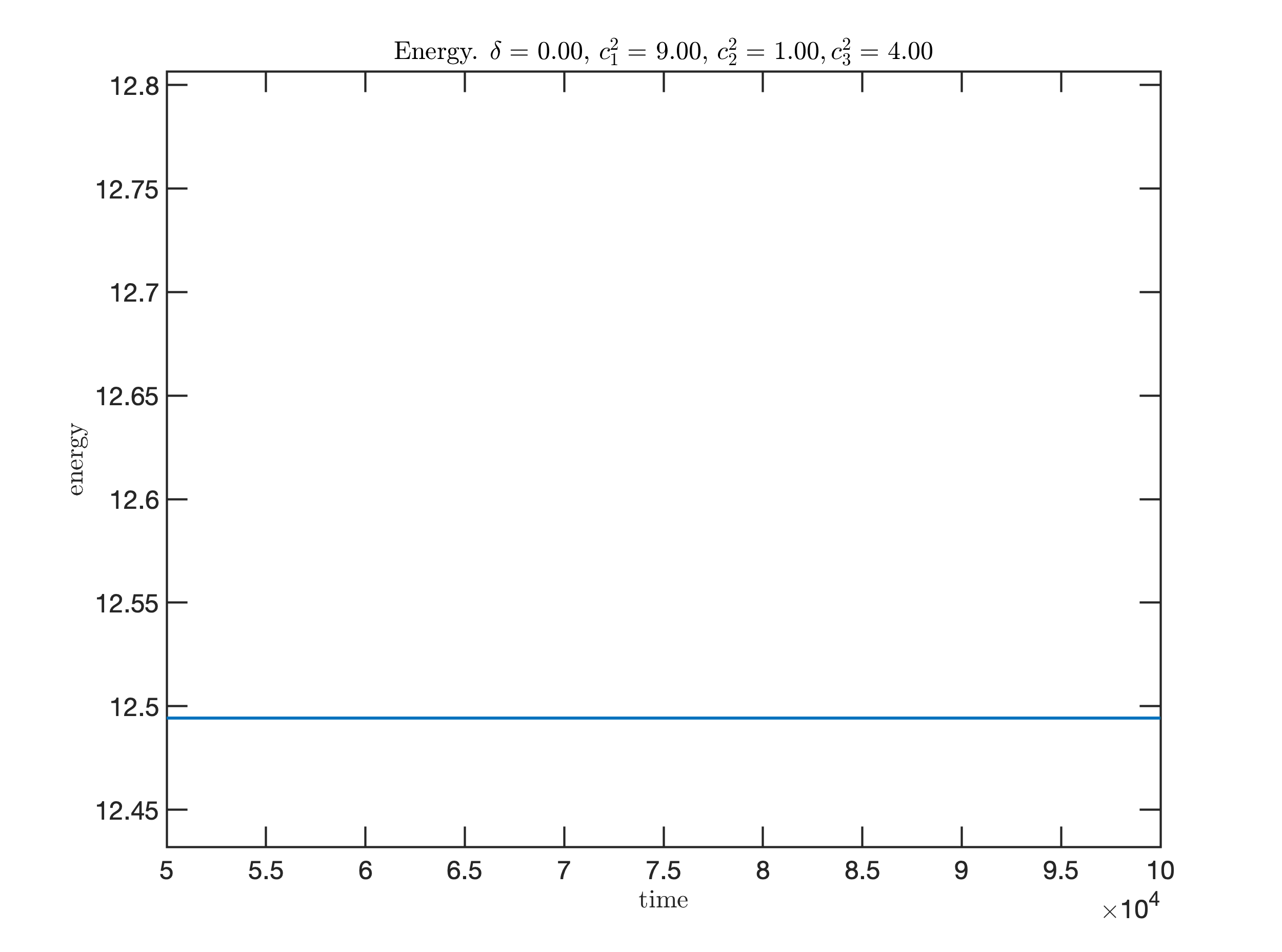
c No damping/different speed

Figure 3. No damping

Let $\displaystyle C^{2}_{1}=C_{2}^{2}=C_{3}^{2}=1$.
Case 1. No damping: conservation of the total energy. When $\displaystyle\delta=0$, Figure 3 shows that the total energy is conserved along time. Thus, this numerical test shows that in the absence of the damping term, the total energy is completely conserved. Consequently, the numerical scheme (2.16) does not produce any numerical dissipation and therefore the numerical behavior observed is only due to the considered model. Indeed, in the case of different propagation speed, numerical tests show also conservation of the energy in the absence of the damping, i.e., when $\displaystyle\delta=0$ (see for instance Figure 3).

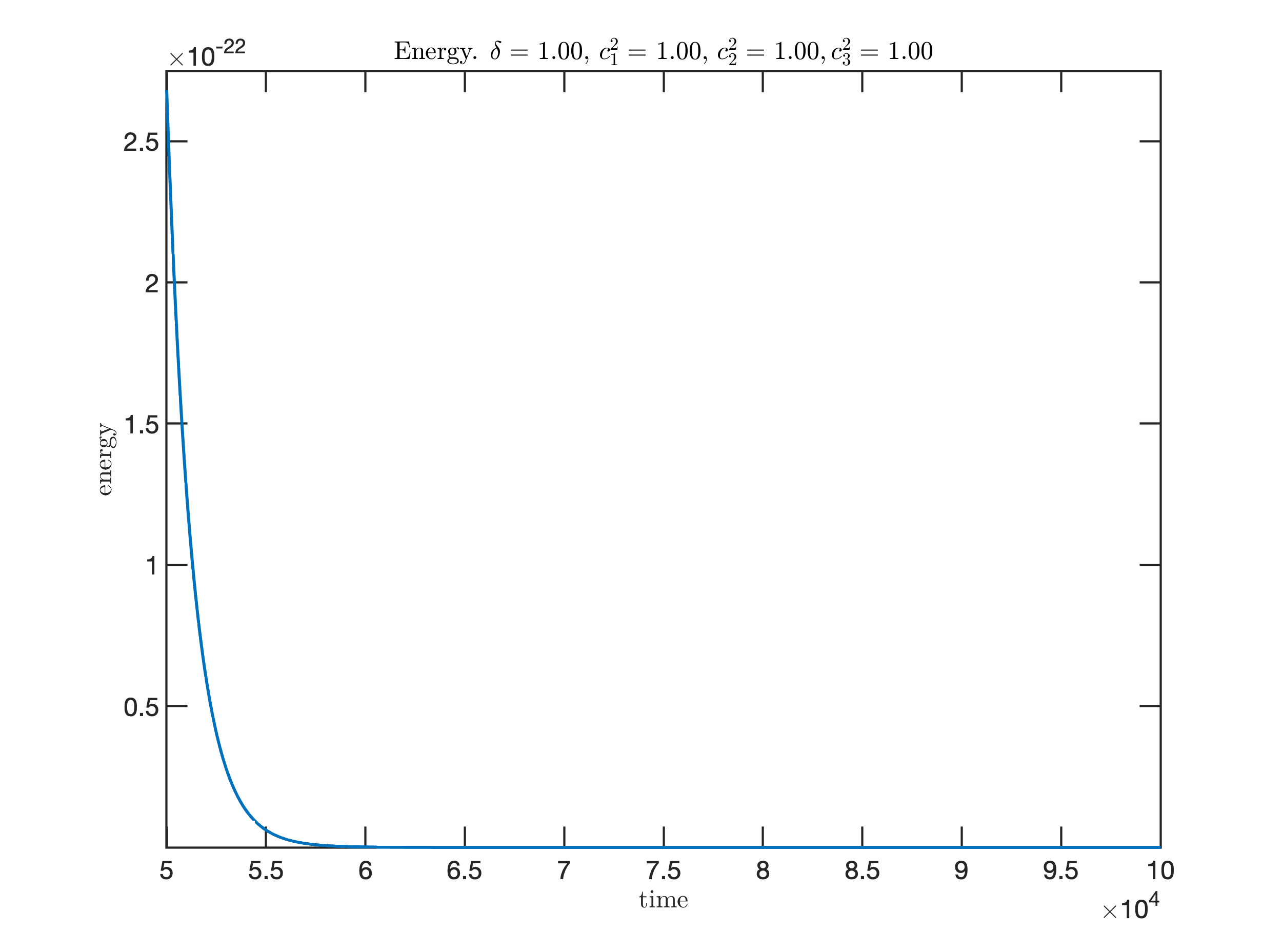
a Energy

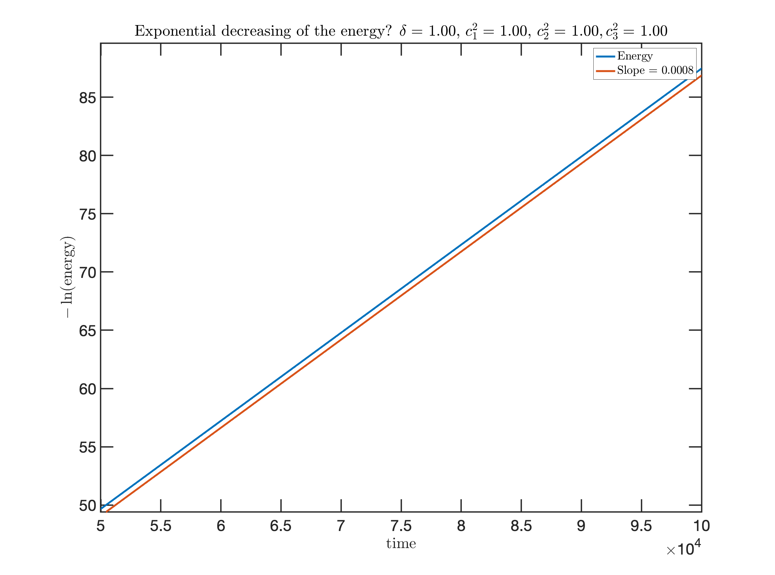
b Exponential decay

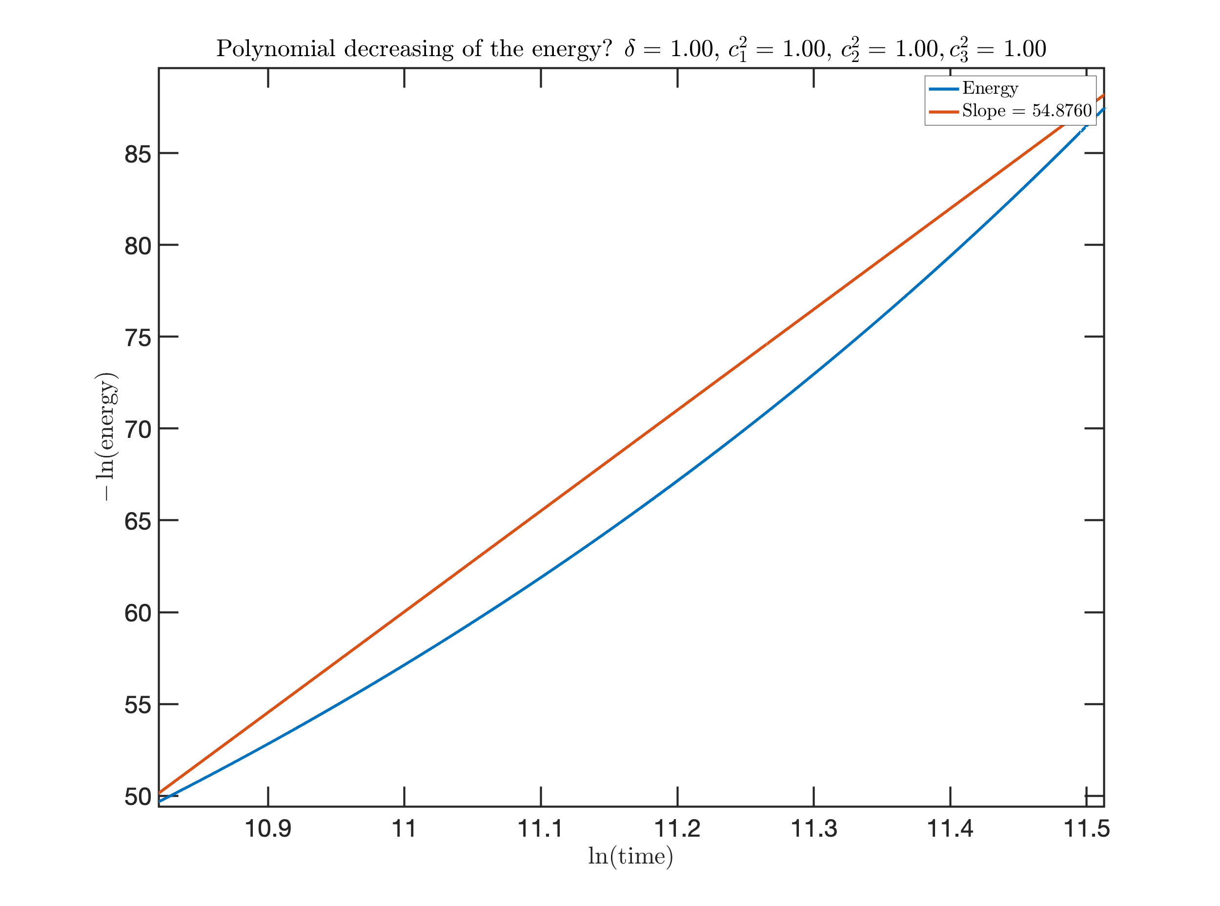
c Polynomial decay?

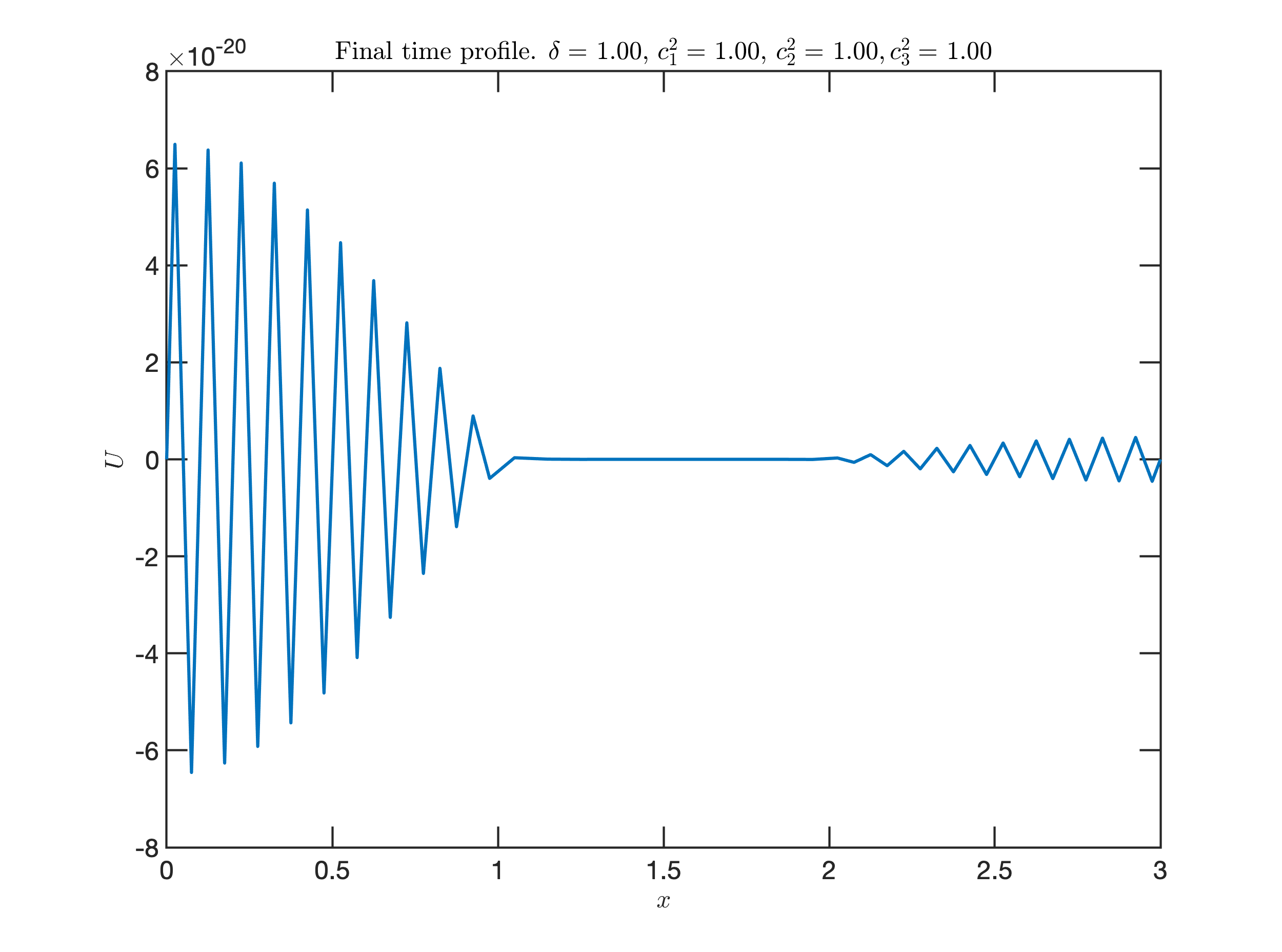
d Final time profile

Figure 4. Long time behavior when $\displaystyle C_{1}^{2}=C_{2}^{2}=C_{3}^{2}=1$

Case 2. Exponential stability. When $\displaystyle\delta=1$, Figure 4-a shows that the total energy goes to zero as $\displaystyle t\to\infty$, and thus we have dissipation. First, for a graph in $\displaystyle\ln$-$\displaystyle\ln$ scale, there is a an energy decay of order $\displaystyle t^{-\alpha}$, whereas, for a graph of $\displaystyle\ln$-time scale, we obtain an energy decay of order $\displaystyle e^{-\omega t}$. By simple linear regression (least squares), Figure 4-c shows that the polynomial decay of the energy is very fast ($\displaystyle\alpha\simeq 54.8760$) and thus we deduce that the energy decays faster than polynomial. In fact, we can observe from Figure 4-b an exponential decay, as the graph of $\displaystyle-\ln(E(t))$ versus time $\displaystyle t$ plots a straight line. By simple linear regression (least squares), we obtain the rate of decay numerically ($\displaystyle\omega\simeq 0.0008$) and it is found to be very small. However, the final time profile confirms that $\displaystyle U$ is small but it shows that high frequencies are not completely controlled (see Figure 4-d).

5.2. Different speed of propagation

In this part, we aim to verify the theoretical results obtained in [9]. To this end, we consider several cases and we obtain the decay rates numerically by simple linear regression (least squares).
Case 1. ($\displaystyle C_{1}>C_{3}>C_{2}$) Polynomial stability. Set $\displaystyle C_{1}^{2}=9,\ C_{2}^{2}=1,\ C_{3}^{2}=4$ and $\displaystyle\delta=1$. Since the final time is large, we show two figures for the energy, the first one is for $\displaystyle t=0$ to $\displaystyle t=100$ and the second one represents the energy from $\displaystyle T/2$ till $\displaystyle T$. Indeed, Figure 5 shows that the total energy is decreasing and goes finally to zero, and thus we look for an exponential or polynomial decay. The graph of $\displaystyle-\ln(E(t))$ versus $\displaystyle t$ plots a curve of the decay of the energy with a very small coefficient ($\displaystyle\omega=0.0001$) which shows that the energy decays slower than exponential (see Figure 5-c). However, Figure 5-d plots the graph of $\displaystyle-\ln(E(t))$ versus $\displaystyle\ln(t)$ which permits to show that $\displaystyle E(t)$ tends to zero as $\displaystyle 1/t^{\alpha}$ with $\displaystyle\alpha\simeq 4.17$, since the curve is asymptotically a straight line. Finally, the final time profile confirms that $\displaystyle U$ is small but also shows that high frequencies are not completely controlled (see Figure 5-e).
Case 2. ($\displaystyle C_{2}>C_{1}>C_{3}$) Polynomial stability. Set $\displaystyle C_{1}^{2}=2,\ C_{2}^{2}=4,\ C_{3}^{2}=0.25$ and $\displaystyle\delta=1$. Similarly, since the final time is large, we show two figures for the energy, the first one is for $\displaystyle t=0$ to $\displaystyle t=100$ and the second one represents the energy from $\displaystyle T/2$ till $\displaystyle T$. Under the same discussion, Figure 6 shows that $\displaystyle E(t)$ tends to zero as $\displaystyle 1/t^{\alpha}$ with $\displaystyle\alpha\simeq 4.4608$. Also, the final time profile confirms that $\displaystyle U$ is small, although the high frequencies are not completely controlled, especially at the beginning of the experiment.
Case 3. ($\displaystyle C_{3}>C_{2}>C_{1}$) Polynomial stability. Set $\displaystyle C_{1}^{2}=2,\ C_{2}^{2}=4,\ C_{3}^{2}=6$ and $\displaystyle\delta=1$. Figure 7 shows that the total energy goes finally to zero. Therefore, to explore the speed of convergence to zero, we plot similarly the graph of $\displaystyle-\ln(E(t))$ versus time and the graph of $\displaystyle-\ln(E(t))$ versus $\displaystyle\ln(t)$. Figure 7-c permits to show that the energy decays slower than exponential ($\displaystyle\omega=0.0005$), and hence we look for a polynomial decay. As a result, $\displaystyle E(t)$ tends to zero as $\displaystyle 1/t^{\alpha}$ with $\displaystyle\alpha\simeq 3.3990$ (see Figure 7-d where the graph is asymptotically a straight line). Finally, the final time profile confirms that $\displaystyle U$ is small but it shows that high frequencies are not completely controlled.
Case 4. ($\displaystyle C_{1}=C_{3}$) Polynomial stability. Set $\displaystyle C_{1}^{2}=C_{3}^{2}=2,\ C_{2}^{2}=4$ and $\displaystyle\delta=1$. Since Figure 8 shows that the total energy goes finally to zero, then we intent to study the speed of convergence to zero. Using the same argument, Figure 8-c permits to show that the energy decays slower than exponential ($\displaystyle\omega=0.0006$), while Figure 8-d states that $\displaystyle E(t)$ tends to zero as $\displaystyle 1/t^{\alpha}$ with $\displaystyle\alpha\simeq 4.4350$. Finally, the final time profile confirms that although $\displaystyle U$ is small, high frequencies are not completely controlled.

Remark 5.

When the propagation speeds are not equal, we obtain a polynomial decay of the energy with slight different rates. However, in some cases, we get a numerical polynomial convergence better than $\displaystyle t^{-4},$ but it will probably be $\displaystyle t^{-4}$ if we increase the time. In this test, we do not perform very long simulation to confirm, for reason of computation time.

Remark 6.

Under the same speed of propagation ($\displaystyle C_{1}^{2}=C_{2}^{2}=C_{3}^{2}=1$), the exponential decay rate depends on the size of the domain where the Kelvin-Voigt damping is acting. In fact, let $\displaystyle\alpha=0.1,\ \beta=2.9$ and choose $\displaystyle N_{\alpha}=N_{\beta}=4,\ N=100$ so that $\displaystyle h_{\alpha}=h_{\beta}=0.025,\ h=0.028$. Also, set $\displaystyle T=100$ and $\displaystyle\mathcal{N}=4000$ such that $\displaystyle\Delta t=\frac{T}{\mathcal{N}}=\textrm{CFL}\times\Delta x$. Figure 9 shows that $\displaystyle E(t)$ decays exponentially to zero with $\displaystyle\omega=0.4312$, and thus, the exponential decreasing rate increases as we add more viscoelastic material. Moreover, the final time profile shows that the high frequency oscillations are exponentially dissipated after a while.

6. Conclusions

As announced, we have constructed a finite volume (explicit or implicit) space discretisation for the transmission problem of a 1-D wave equation with non smooth wave speed an localized Kelvin-Voigt damping. We have proved that the discrete solution converges to the continuous weak solution when the discretisation step size goes to zero. Moreover, from the numerical experiments, we have also proved that the decay rate of the discrete solution towards the null solution when damping acts and the speeds are equal or different is in compliance with the theoretical study performed by two of the authors in [9].

In the future, the investigation of the order of the space discretisation could also be performed. We expect a first order discretisation in space since the elliptic part is of first order. It could be done by a careful numerical analysis but also by performing numerical experiments.

a Initial profile

b No damping/equal speed

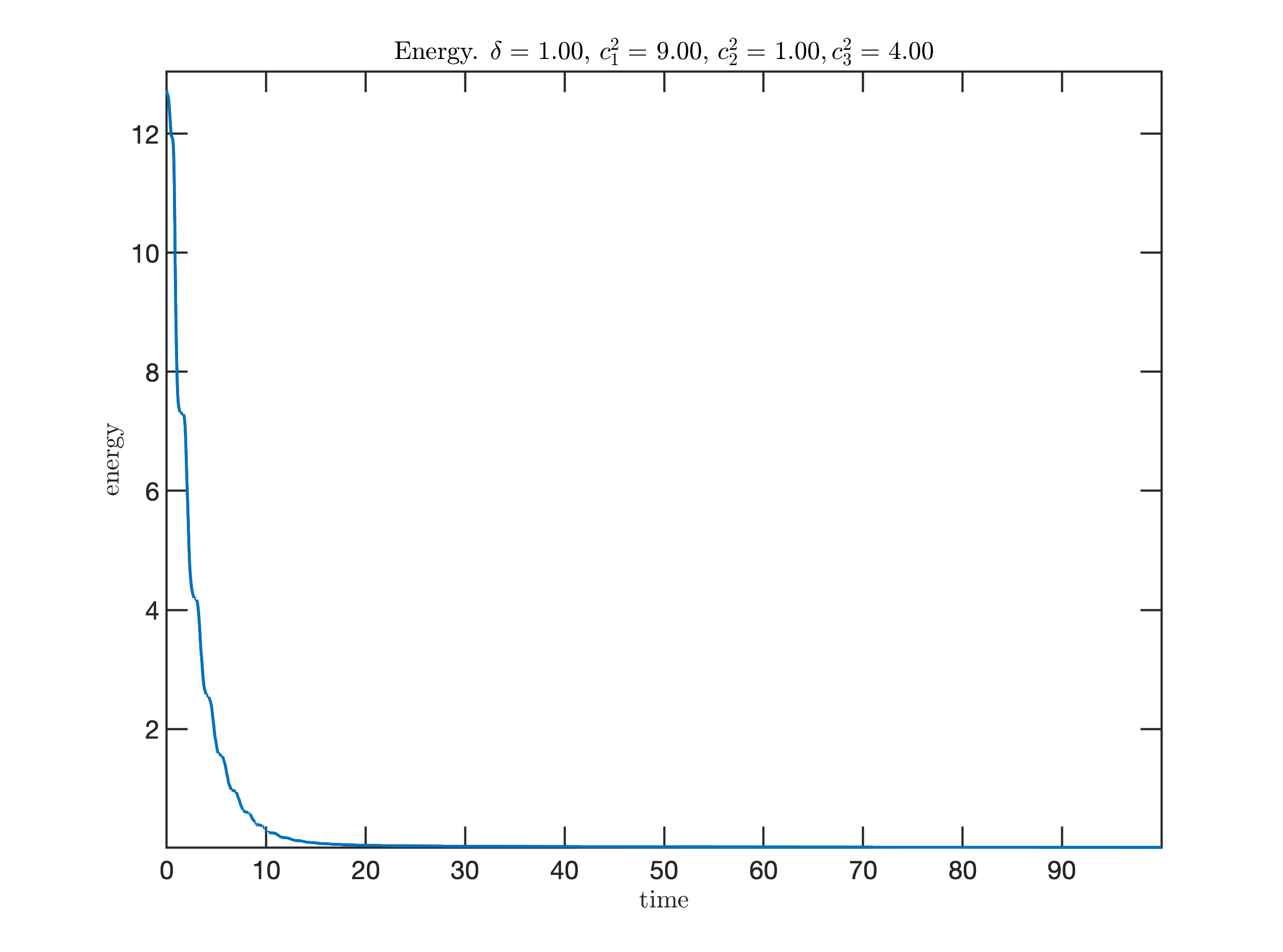
a Energy ($\displaystyle t=0$ till $\displaystyle t=100$)

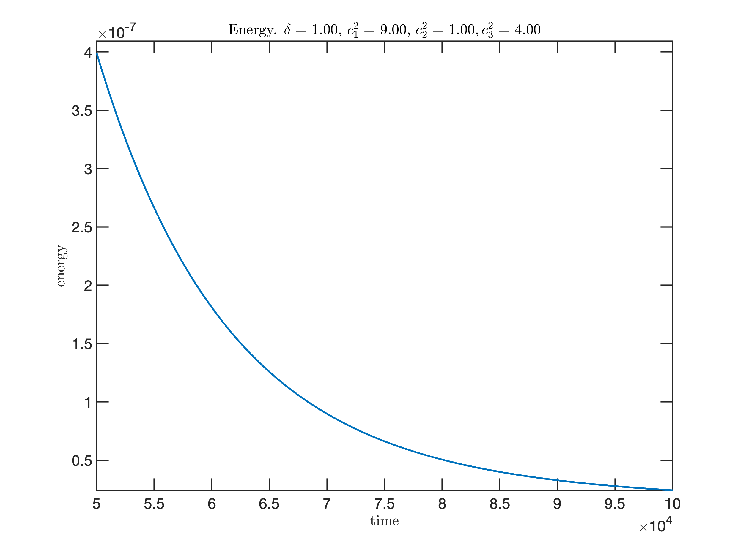
b Energy ($\displaystyle T/2$ till $\displaystyle T$)

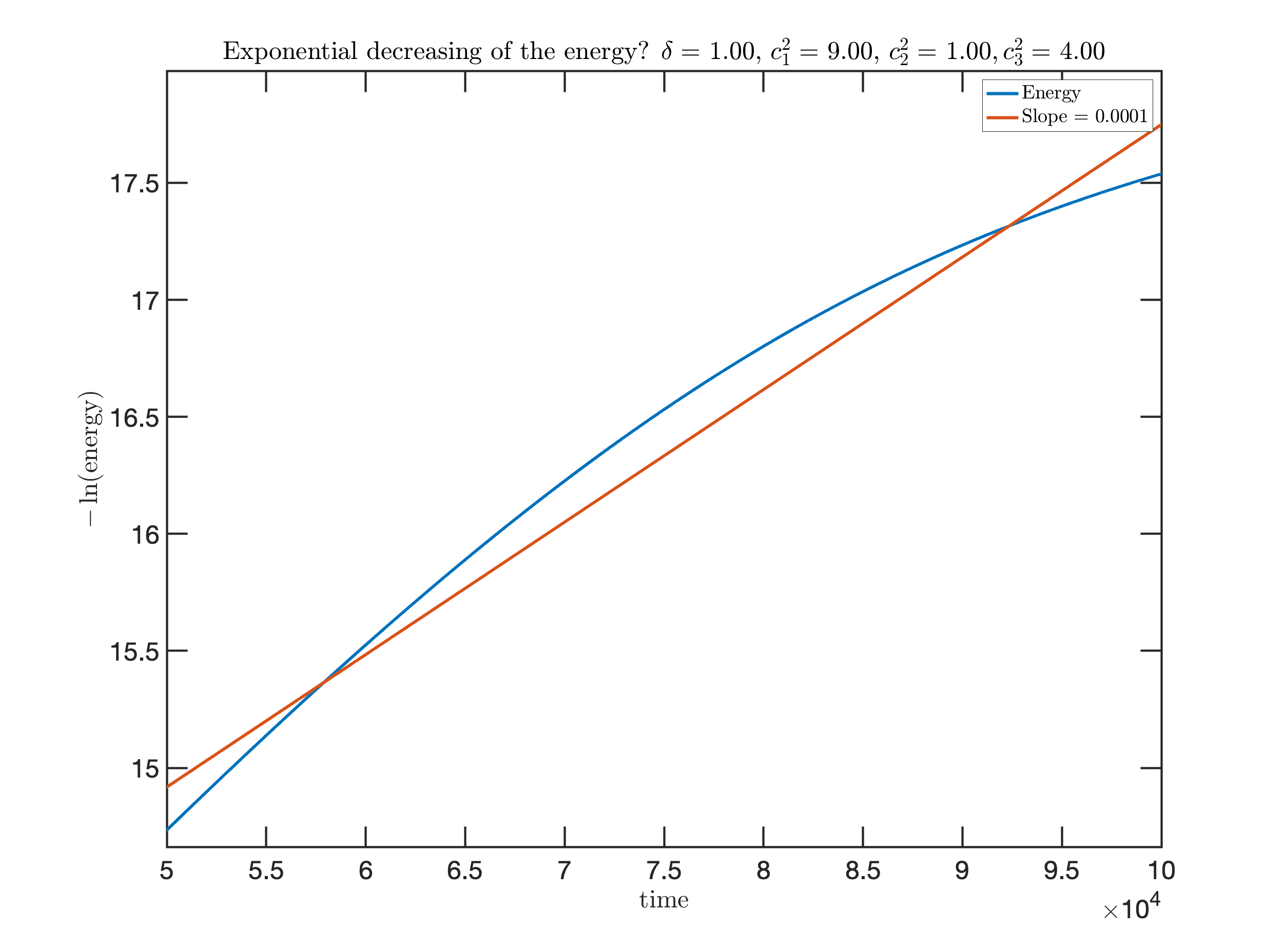
c Exponential decay?

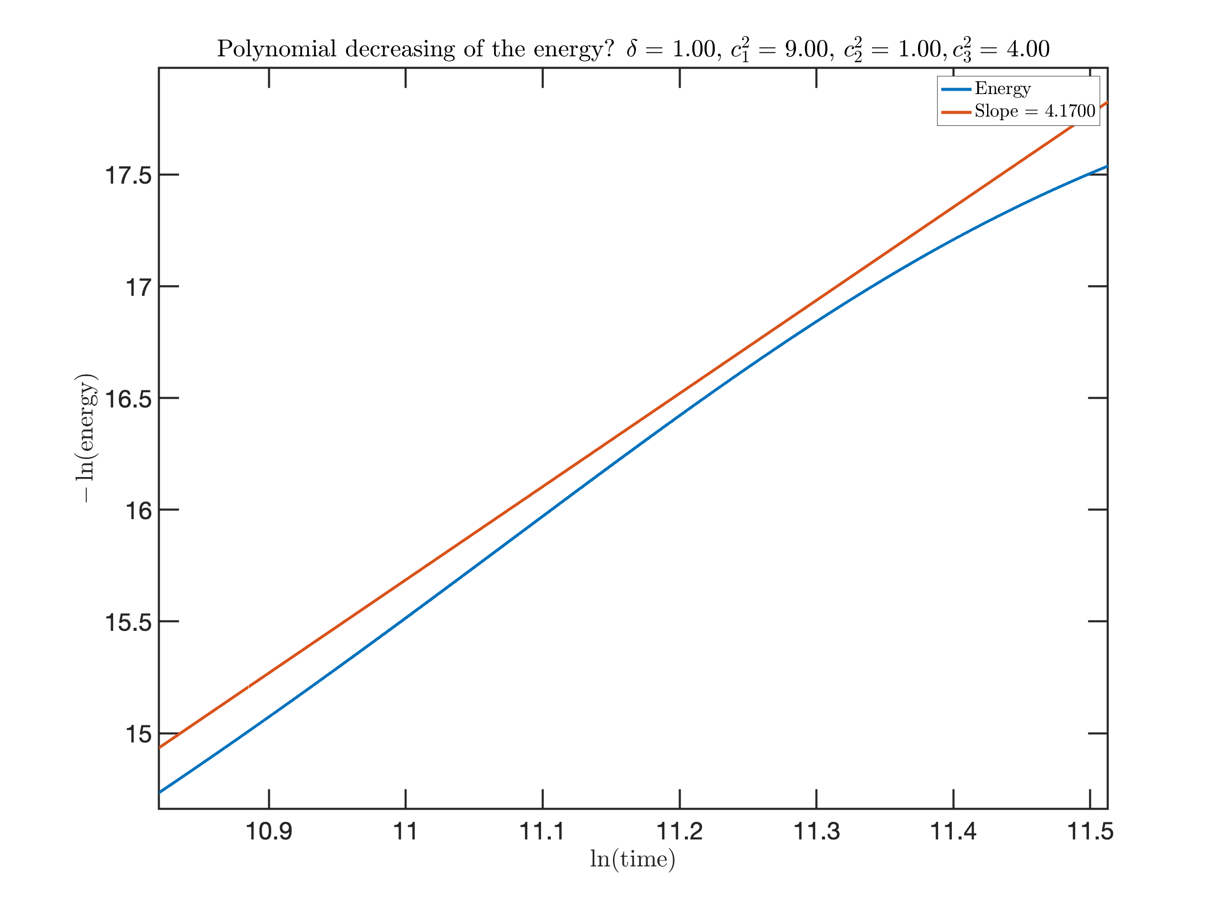
d Polynomial decay

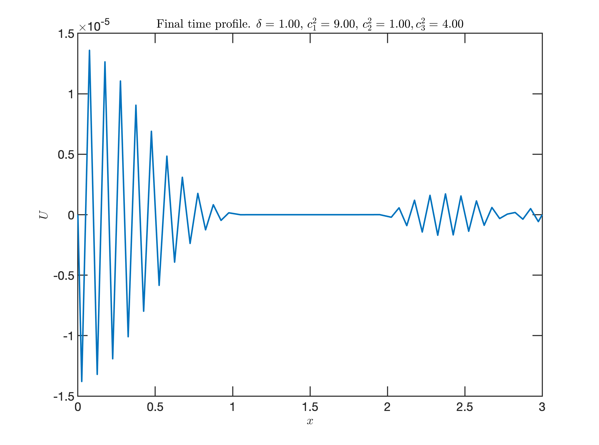
e Final time profile

Figure 5. Long time behavior when $\displaystyle C_{1}^{2}=9,\ C_{2}^{2}=1,\ C_{3}^{2}=4$

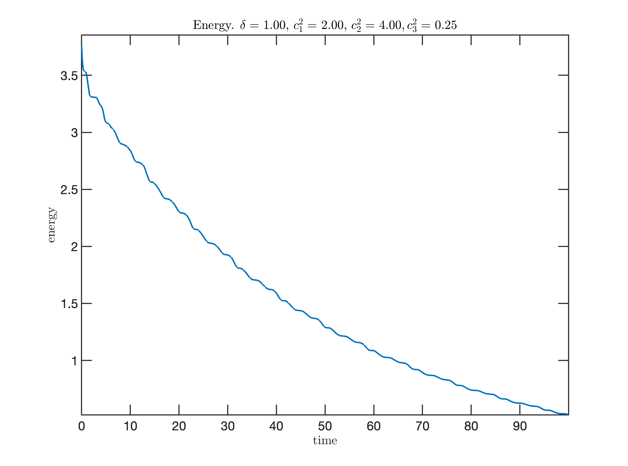
a Energy ($\displaystyle t=0$ till $\displaystyle t=100$)

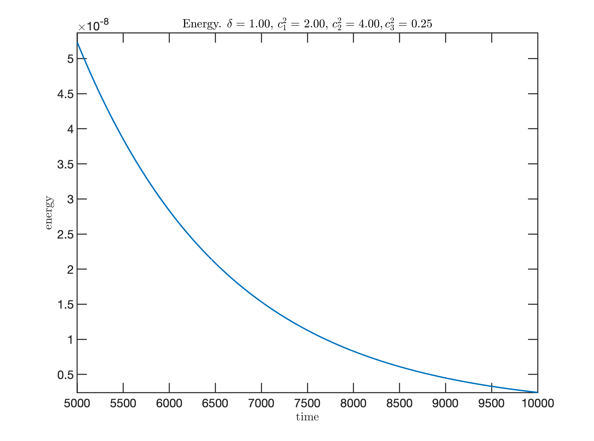
b Energy ($\displaystyle T/2$ till $\displaystyle T$)

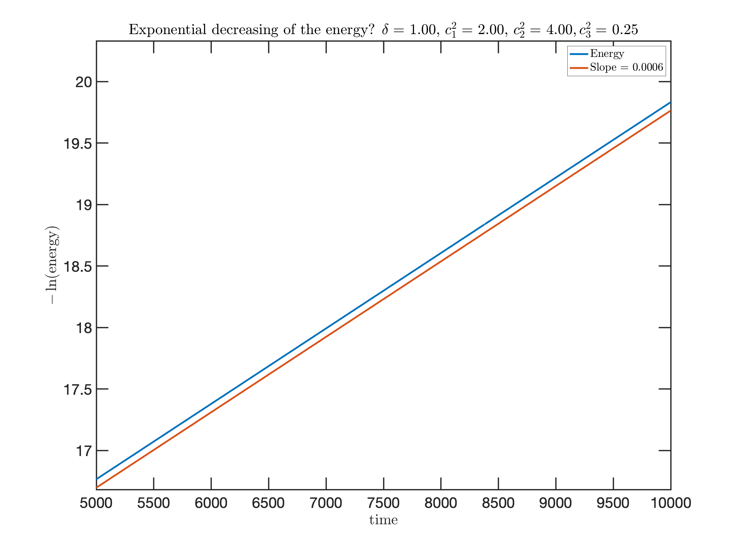
c Exponential decay?

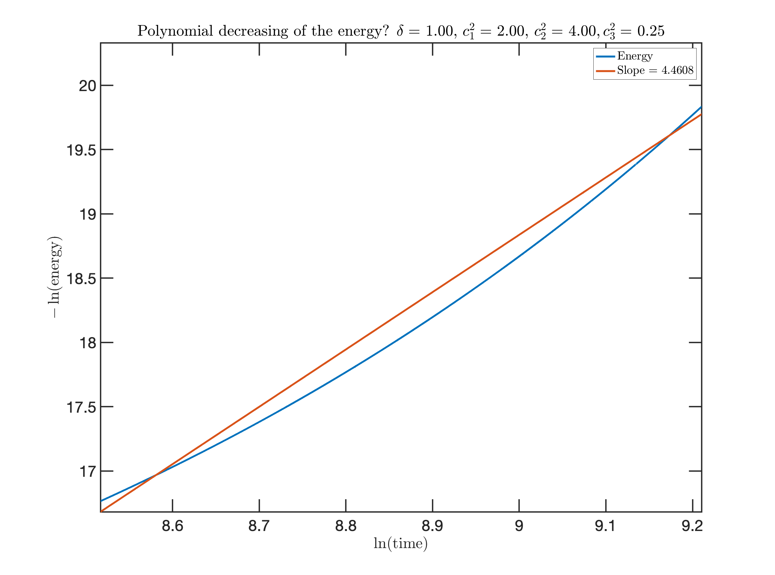
d Polynomial decay

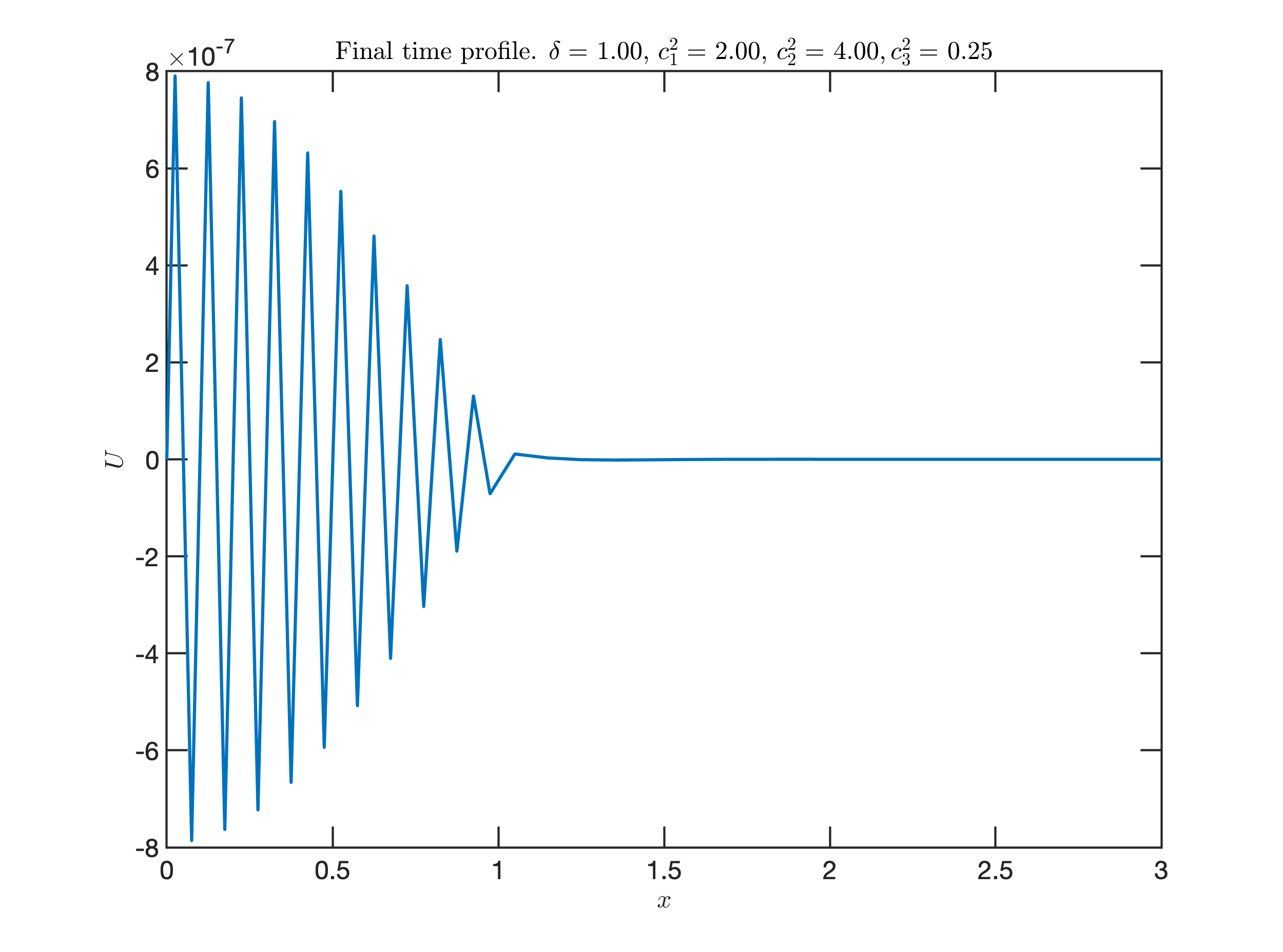
e (e) Final time profile

Figure 6. Long time behavior when $\displaystyle C_{1}^{2}=2,\ C_{2}^{2}=4,\ C_{3}^{2}=0.25$

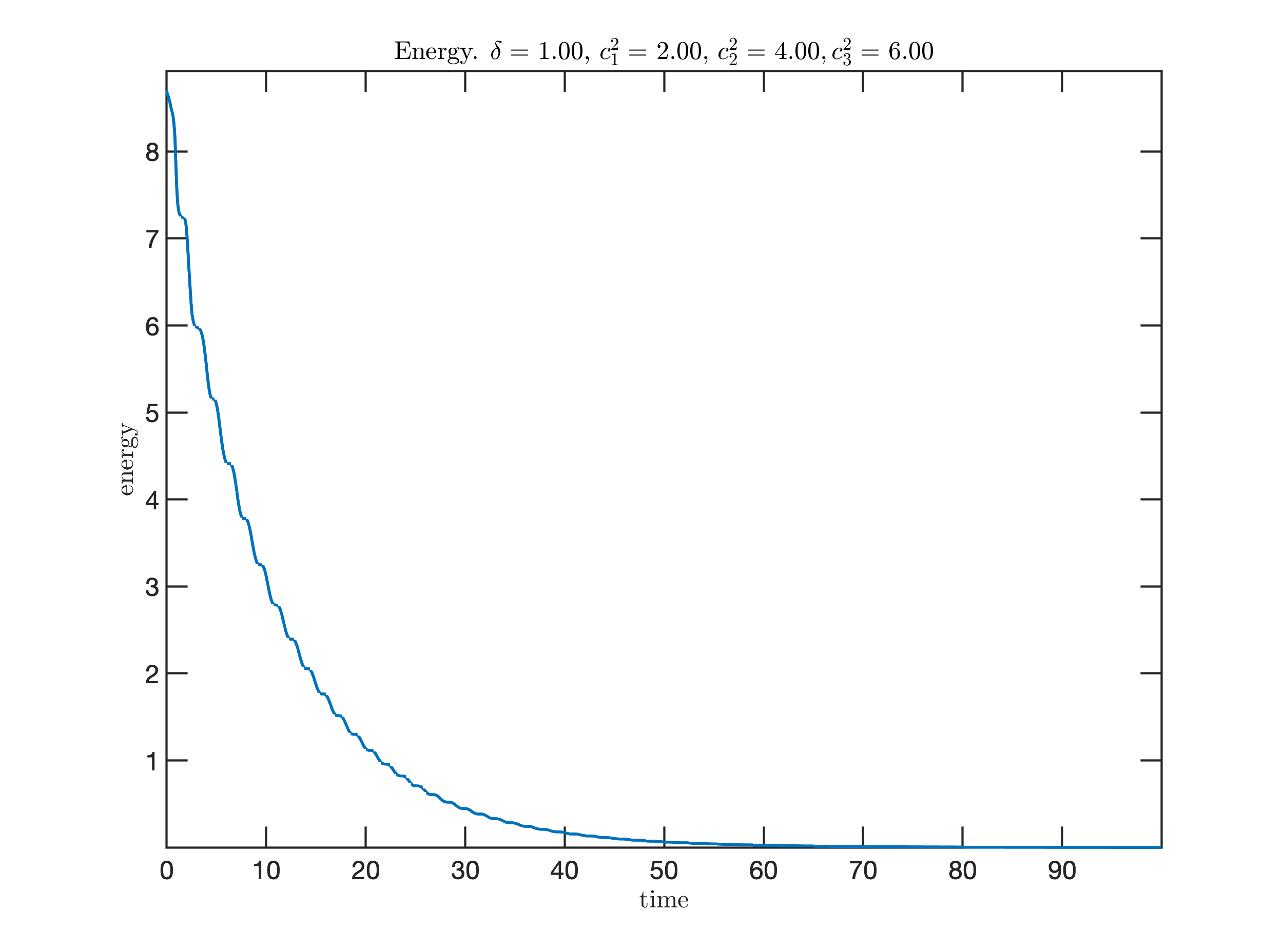
a Energy ($\displaystyle t=0$ till $\displaystyle t=100$)

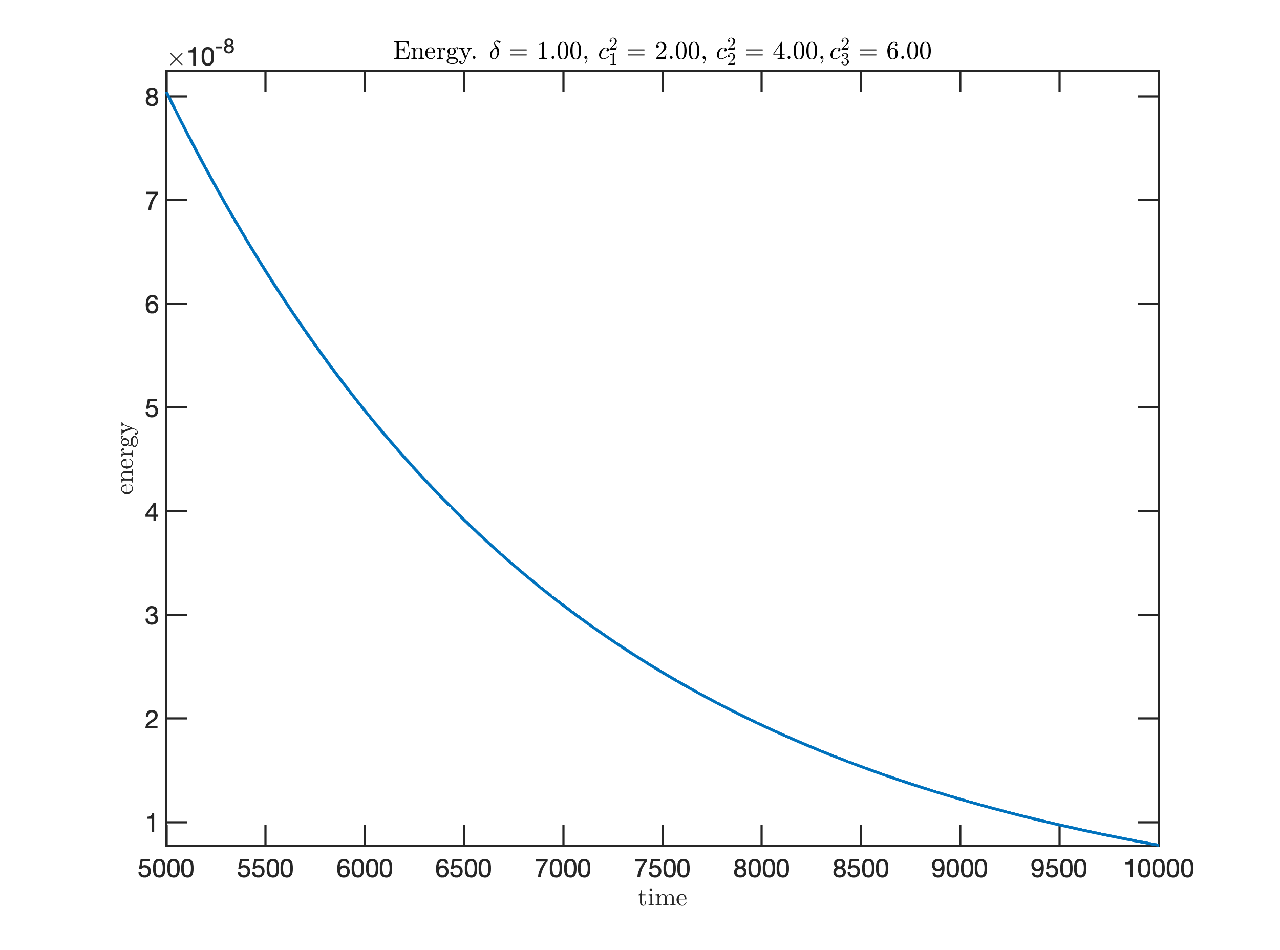
b Energy ($\displaystyle T/2$ till $\displaystyle T$)

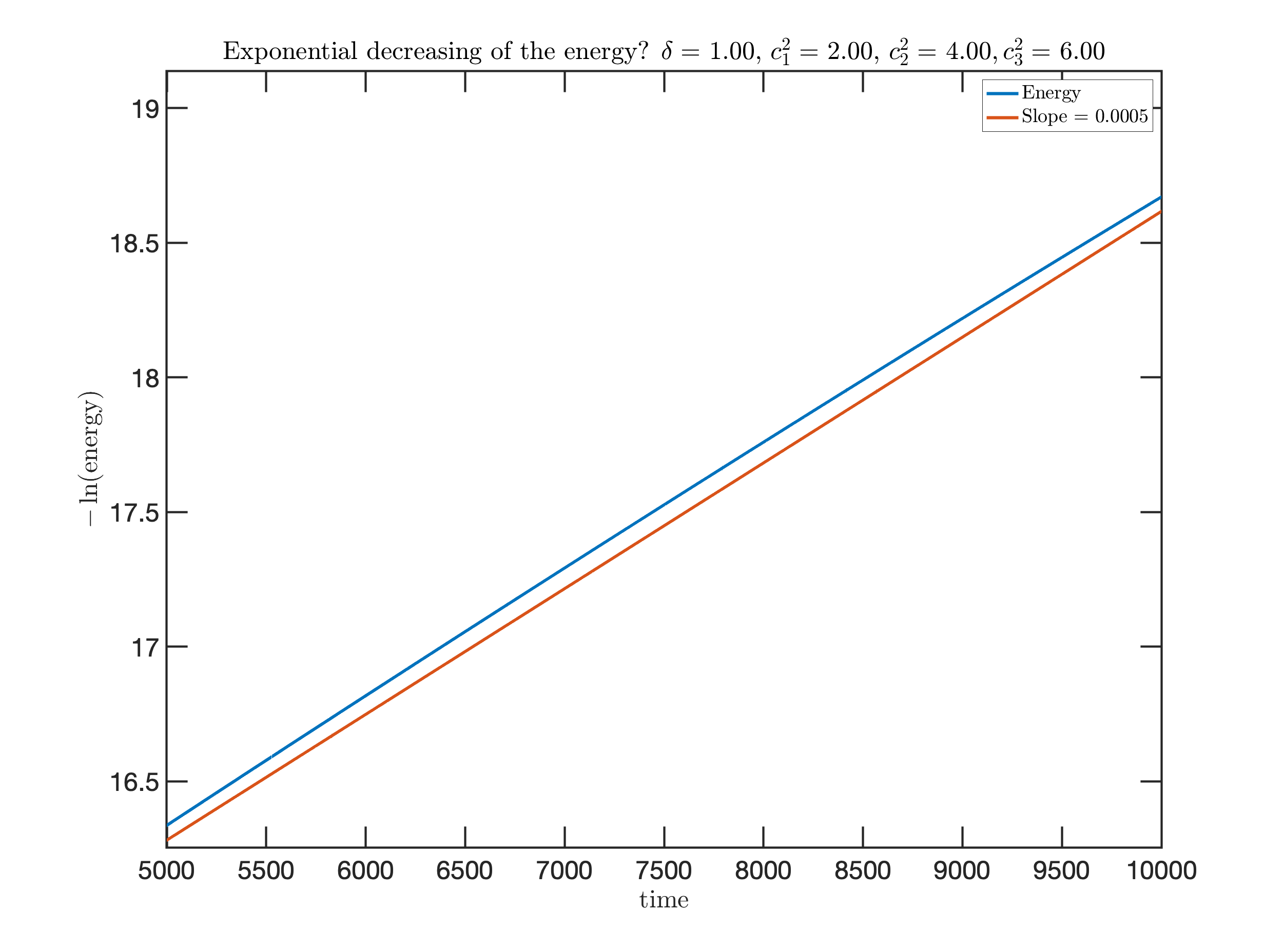
c Exponential decay?

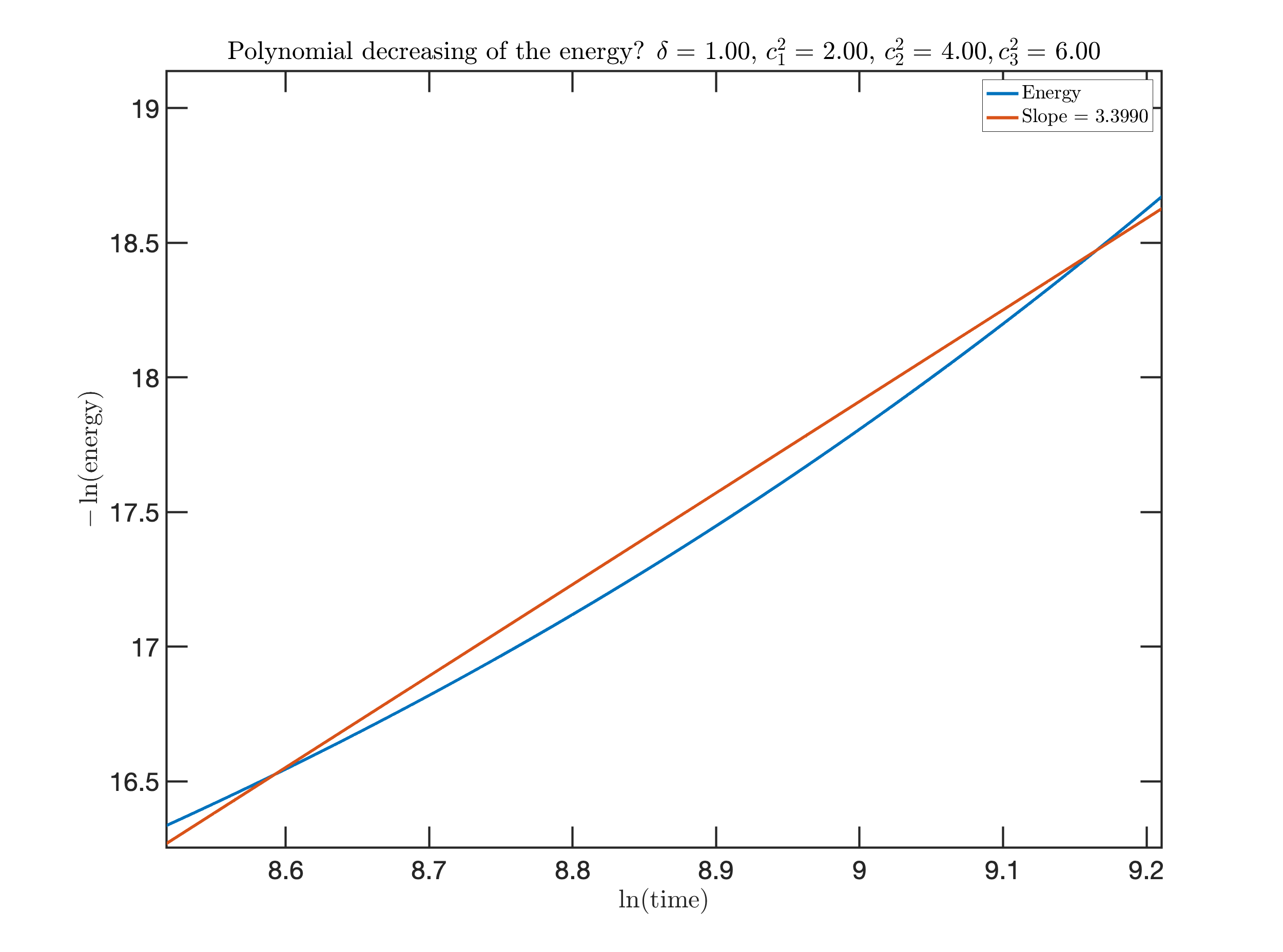
d Polynomial decay

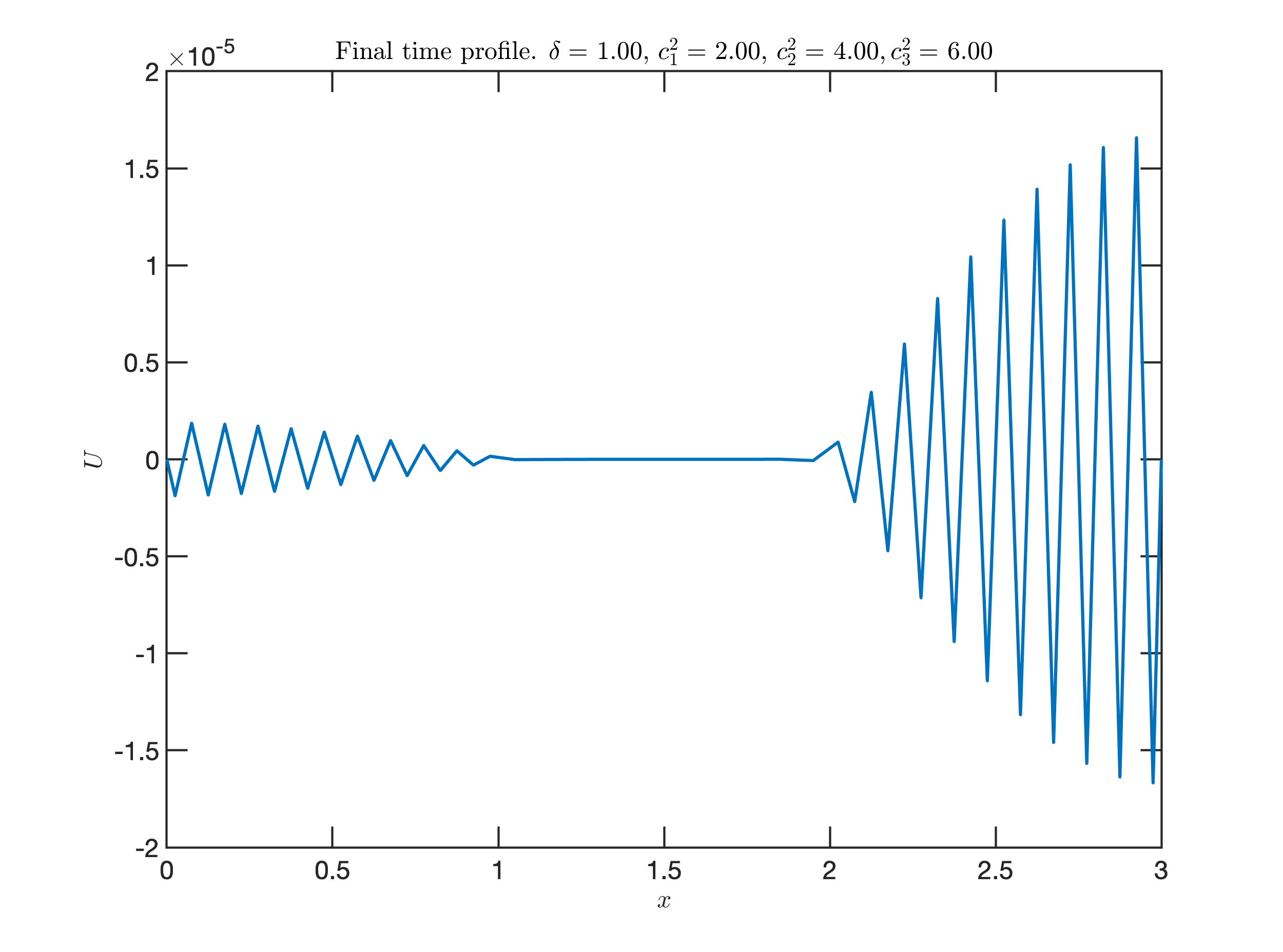
e (e) Final time profile

Figure 7. Long time behavior when $\displaystyle C_{1}^{2}=2,\ C_{2}^{2}=4,\ C_{3}^{2}=6$

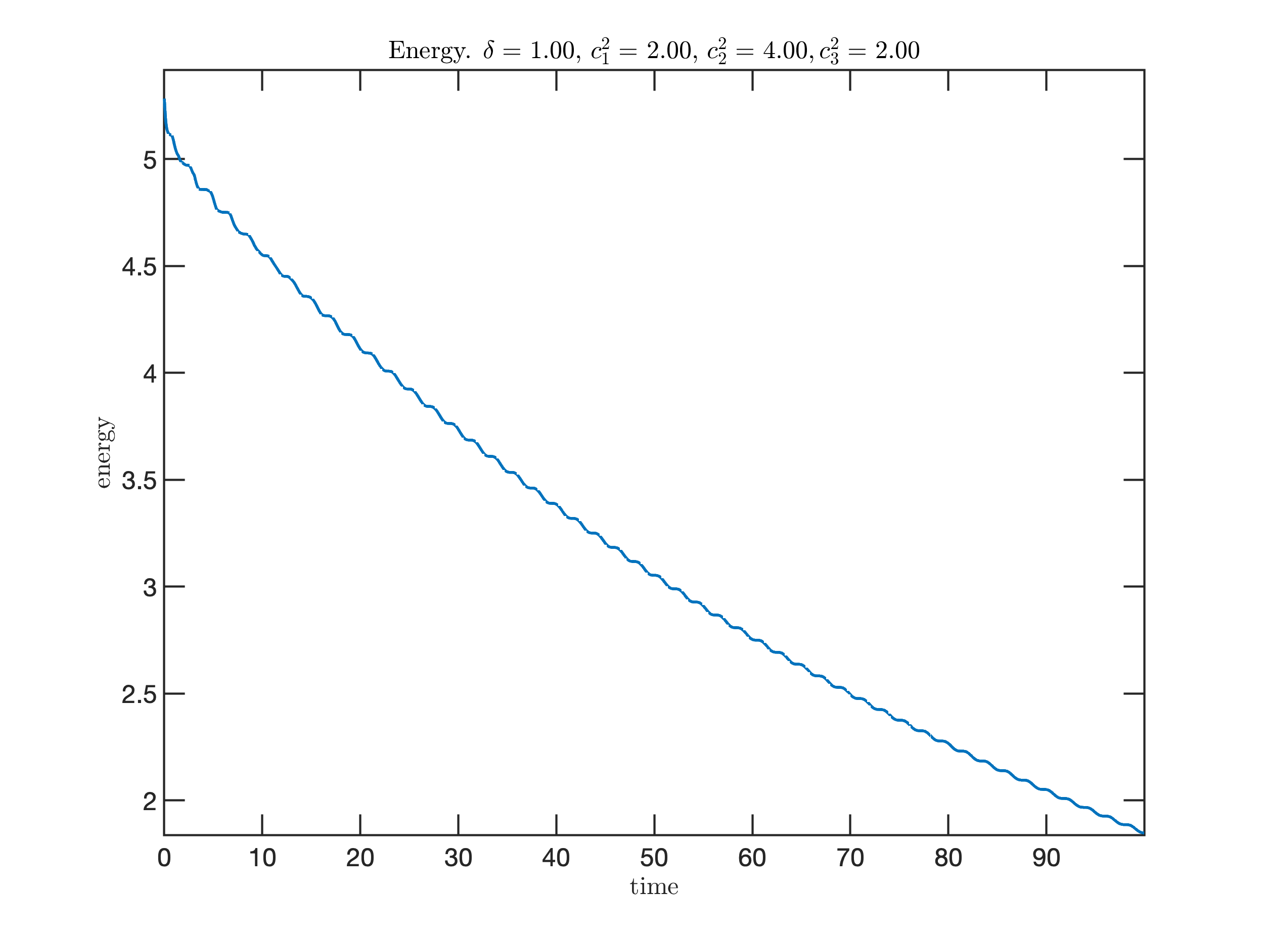
a Energy ($\displaystyle t=0$ till $\displaystyle t=100$)

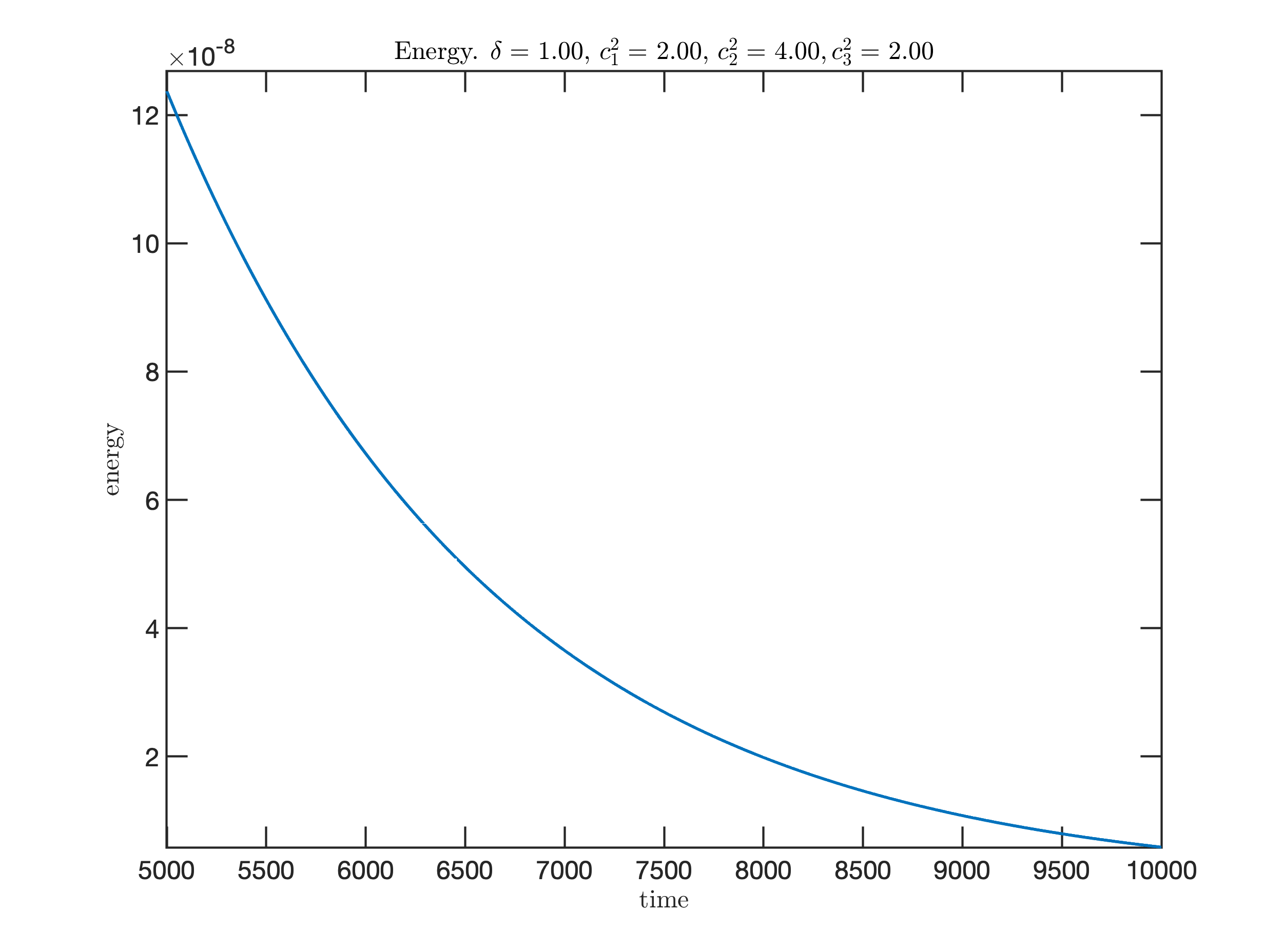
b Energy ($\displaystyle T/2$ till $\displaystyle T$)

c Exponential decay?

d Polynomial decay

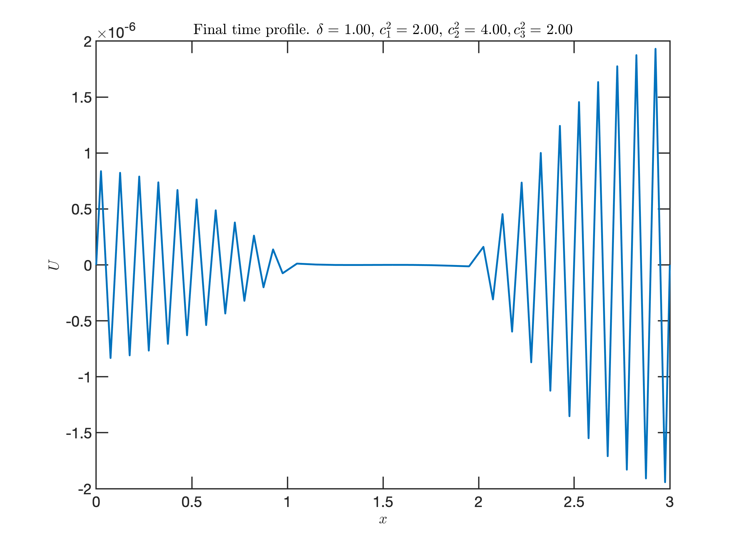
e (e) Final time profile

Figure 8. Long time behavior when $\displaystyle C_{1}^{2}=C_{3}^{2}=2,\ C_{2}^{2}=4$

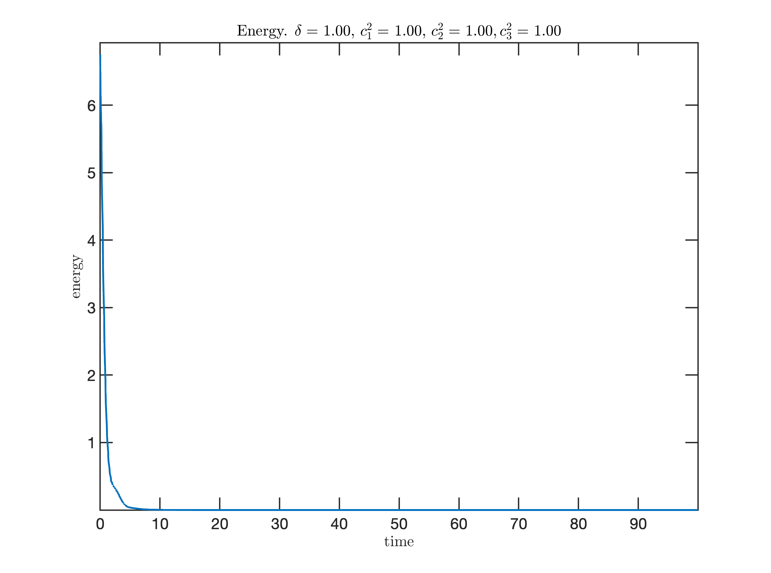
a Energy ($\displaystyle t=0$ till $\displaystyle t=100$)

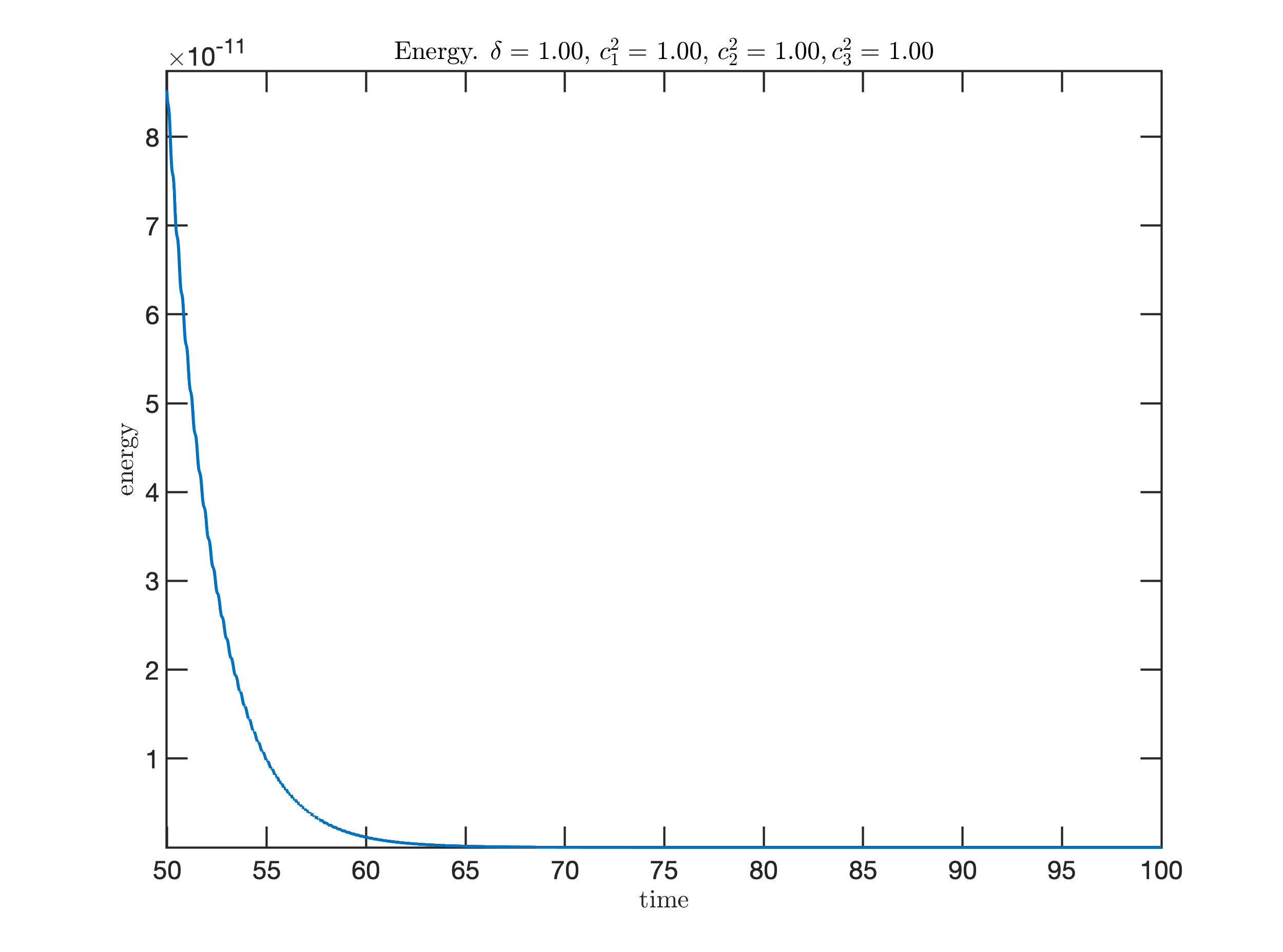
b Energy ($\displaystyle T/2$ till $\displaystyle T$)

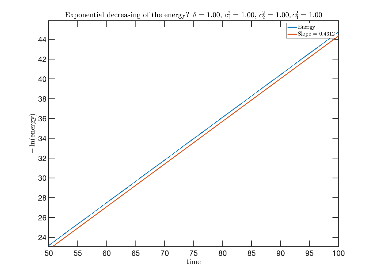
c Exponential decay

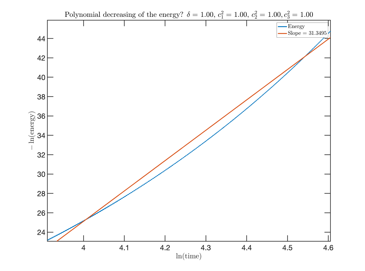
d Polynomial decay?

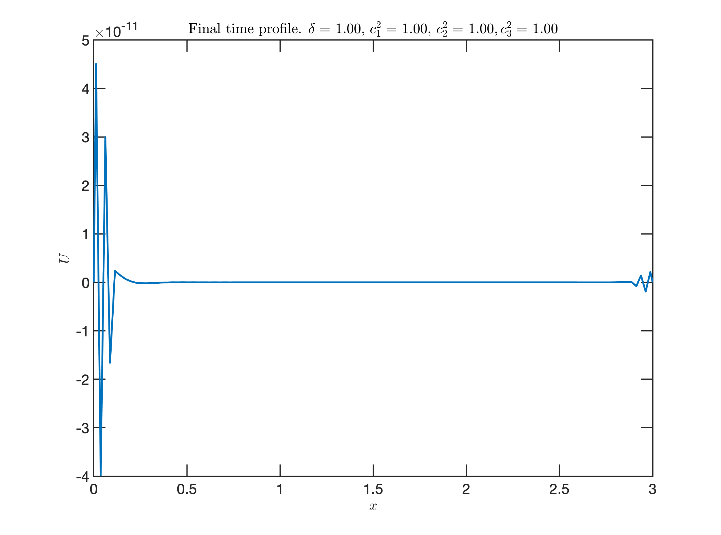
e Final time profile

Figure 9. Exponential decay under same propagation speed and more viscoelastic material

References

- [1] M. Alves, J. M. Rivera, M. Sepúlveda, and O. V. Villagrán, The Lack of Exponential Stability in Certain Transmission Problems with Localized Kelvin–Voigt Dissipation, SIAM Journal on Applied Mathematics, 74 (2014), pp. 345–365.
- [2] M. Alves, J. M. Rivera, M. Sepúlveda, O. V. Villagrán, and M. Z. Garay, The asymptotic behavior of the linear transmission problem in viscoelasticity, Mathematische Nachrichten, 287 (2013), pp. 483–497.
- [3] K. Ammari, F. Hassine, and L. Robbiano, Stabilization for the wave equation with singular kelvin-Voigt damping, Archive for Rational Mechanics and Analysis, 236 (2019), pp. 577–601.
- [4] K. Ammari, Z. Liu, and F. Shel, Stability of the wave equations on a tree with local Kelvin–Voigt damping, Semigroup Forum, (2019).
- [5] R. Eymard, T. Gallouët, and R. Herbin, Finite volume methods, in Handbook of numerical analysis, Vol. VII, vol. VII of Handb. Numer. Anal., North-Holland, Amsterdam, 2000, pp. 713–1020.
- [6] R. Eymard, A. Handlovicová, and K. Mikula, Study of a finite volume scheme for the regularized mean curvature flow level set equation, Ima Journal of Numerical Analysis, 31 (2011), pp. 813–846.
- [7] F. Gao and C.-M. Chi, Unconditionally stable difference schemes for a one-space-dimensional linear hyperbolic equation, Applied Mathematics and Computation, 187 (2007), pp. 1272–1276.
- [8] M. Ghader, R. Nasser, and A. Wehbe, Stability results for an elastic/viscoelastic wave equation with localized Kelvin-Voigt damping and with an internal or boundary time delay, Asymptotic Analysis, (2020), pp. 1–57.
- [9] M. Ghader, R. Nasser, and A. Wehbe, Optimal polynomial stability of a string with locally distributed Kelvin-Voigt damping and nonsmooth coefficient at the interface, Math. Methods Appl. Sci., 44 (2021), pp. 2096–2110.
- [10] G. H. Golub and G. A. Meurant, Résolution numérique des grands systèmes linéaires, vol. 49 of Collection de la Direction des Études et Recherches d’Électricité de France [Collection of the Department of Studies and Research of Électricité de France], Éditions Eyrolles, Paris, 1983.
- [11] B. Hamilton, Finite Difference and Finite Volume Methods for Wave-based Modelling of Room Acoustics, PhD thesis, University of Edinburgh, 2016.
- [12] S. Larsson, V. Thomée, and L. B. Wahlbin, Finite-element methods for a strongly damped wave equation, IMA J. Numer. Anal., 11 (1991), pp. 115–142.
- [13] R. J. LeVeque, Finite-Volume Methods for Hyperbolic Problems, Cambridge University Press, 2002.
- [14] T. Maryati, J. Muñoz Rivera, A. Rambaud, and O. Vera, Stability of an N-component timoshenko beam with localized Kelvin–Voigt and frictional dissipation, Electronic Journal of Differential Equations, 2018 (2018).
- [15] C. Raposo, W. Bastos, and J. Avila, A Transmission Problem for Euler-Bernoulli beam with Kelvin-Voigt Damping, Applied Mathematics and Information Sciences, 5 (2011), pp. 17–28.
- [16] I. Riečanová and A. Handlovičová, Study of the numerical solution to the wave equation, Acta Math. Univ. Comenian. (N.S.), 87 (2018), pp. 317–332.
- [17] M. A. Rincon and M. Copetti, Numerical analysis for a locally damped wave equation, Journal of Applied Analysis and Computation, 3 (2013), pp. 169–182.
- [18] J. E. M. Rivera, O. V. Villagran, and M. Sepulveda, Stability to localized viscoelastic transmission problem, Communications in Partial Differential Equations, 43 (2018), pp. 821–838.
- [19] T. Sato and S. M. Richardson, Explicit numerical simulation of time-dependent viscoelastic flow problems by a finite element/finite volume method, Journal of Non-Newtonian Fluid Mechanics, 51 (1994), pp. 249 – 275.
- [20] L. Tebou and E. Zuazua, Uniform exponential long time decay for the space semi-discretization of a locally damped wave equation via an artificial numerical viscosity, Numerische Mathematik, 95 (2003), pp. 563–598.
- [21] S. Wang, K. Virta, and G. Kreiss, High order finite difference methods for the wave equation with non-conforming grid interfaces, J. Sci. Comput., 68 (2016), pp. 1002–1028.
- [22] A. Wehbe, , R. Nasser, and N. Noun, Stability of N-D transmission problem in viscoelasticity with localized Kelvin-Voigt damping under different types of geometric conditions, Mathematical Control & Related Fields, 0 (2019), pp. 0–0.
- [23] X. Yu, Z. Ren, Q. Zhang, and C. Xu, A Numerical Method of the Euler-Bernoulli Beam with Optimal Local Kelvin-Voigt Damping, Journal of Applied Mathematics, 2014 (2014), pp. 1–7.
- [24] W. Zhang, Y. Zhuang, and E. T. Chung, A new spectral finite volume method for elastic wave modelling on unstructured meshes, Geophysical Journal International, 206 (2016), pp. 292–307.
- [25] W. Zhang, Y. Zhuang, and L. Zhang, A new high-order finite volume method for 3D elastic wave simulation on unstructured meshes, Journal of Computational Physics, 340 (2017), pp. 534 – 555.