H I absorption line and anomalous dispersion in the radio pulses of PSR B1937+21

Abstract

We use the Five-hundred-meter Aperture Spherical radio Telescope (FAST) to observe the bright millisecond pulsar (MSP) PSR B1937+21 (J1939+2134) and record the data in the band from 1.0 GHz to 1.5 GHz. We measure the neutral hydrogen (H i) emission and absorption lines near 1420 MHz ($\lambda\simeq 21$ cm). We derive the kinematic distance of the pulsar with the H i observation, and update the upper bound of kinematic distance from the previous $14.8\pm 0.9\,\mathrm{kpc}$ in the Outer Arm to the nearer $9.4\pm 0.5\,\mathrm{kpc}$ in the Perseus Arm. By comparing with the archival absorption spectra observed decades ago, we notice possible variations in the absorption spectra towards this pulsar, which corresponds to a possible tiny-scale atomic structure (TSAS) of a few AU in size. We also verify the apparent faster-than-light anomalous dispersion at the H i absorption line of this pulsar previously reported.

1 Introduction

The interaction of the magnetic moments of the electron and proton is at the energy level of $\rm\mu eV$, which leads to the ‘hyperfine splitting’ of energy level between the hydrogen atom ‘triplet’ and ‘singlet’ states. The energy of the triplet state is higher than the singlet state by approximately $6\,\mathrm{\mu eV}$, i.e. 1420.4 MHz. van de Hulst (1945) predicted the 21 cm emission from neutral hydrogen (H i) in the space, which was later detected in 1951 (Ewen & Purcell, 1951; Muller & Oort, 1951). In the astronomical context, H i absorption line was detected a couple years later (Williams & Davies, 1954; Hagen et al., 1954; Hagen & McClain, 1954). It was immediately proposed that the radial velocity of emission and absorption lines, combined with the Galactic rotation curve, can be used to measure the distance of radio sources (Williams & Davies, 1954), which is known as H i kinematic distance. Gomez-Gonzalez & Guelin (1974) and Graham et al. (1974) first applied this method to the determination of pulsar distance. This method measures the distances of the emitting H i clouds in the background and the absorbing ones in the foreground, thus constraining the distance of pulsar between the nearest background and farthest foreground clouds. Several surveys using this method have been published (see Verbiest et al. 2012 for a summary).

Beyond distance measurement, H i observations of pulsars help to resolve interstellar medium (ISM) fluctuations. The angular fluctuations in the H i absorption spectra were firstly discovered in the VLBI observation of the extragalactic source 3C 147 (Dieter et al., 1976), which reflects tiny-scale atomic structure (TSAS, Stanimirović & Zweibel 2018) in the neutral hydrogen atoms (H i) of the ISM. The temporal variations in the H i absorption spectra towards pulsars can also be used to detect TSAS, which was noticed by Clifton et al. 1988 in the absorption spectra of PSR B1821+05. Several surveys were dedicated to the temporal variation of the H i absorption line towards pulsars using recibo Telescope (Frail et al., 1994; Stanimirović et al., 2003; Weisberg & Stanimirović, 2007; Stanimirović et al., 2010), Murriyang Telescope at Parkes Observatory (Johnston et al., 2003), the Green Bank Telescope (GBT, Minter et al. 2005).

The H i energy level also affects the timing of pulsar radio signal around the transition frequency due to the electromagnetic wave propagation, as inferred from Kramers-Kronig relation (e.g., Jackson, 1998). To the leading order, the group velocity of electromagnetic wave propagating in medium is

$$v_{\mathrm{g}}=\frac{\mathrm{d}\omega}{\mathrm{d}k}=\frac{c}{n(\omega)+\omega\frac{\mathrm{d}n}{\mathrm{d}\omega}},$$ (1)

where $\omega$ is the angular frequency of the wave, $n=ck/\omega$ is the refractive index of the medium, and $c$ is the speed of light in vacuum (Jackson, 1998). In most cases, $v_{\mathrm{g}}$ is slower than $c$. However, around absorption lines, the group velocity can be faster than $c$, if $\mathrm{d}n/\mathrm{d}\omega$ is sufficiently negative, i.e. in the strong anomalous dispersion regime (Garrett & McCumber, 1970; Jackson, 1998). It is worth noting that the superluminal propagation (group velocity) around absorption lines does not violate causality. When it happens, the leading edge of a pulse is less attenuated than the trailing edge, thus the peak which defines the group velocity can moves faster than the leading edge (Jackson, 1998). The wide-band and periodic pulses from pulsars can be used to directly measure such the anomalous dispersion of electromagnetic waves in ISM. Indeed, 15 years ago, the pioneer work (Jenet et al., 2010) had detected such the ‘fast-than-light’ propagation phenomenon around the H i  frequency use of the Arecibo data of PSR B1937+21 (J1939+2134). To detect such a phenomenon, one requires radio telescopes of great sensitivity that accurate time of arrivals can be measured for a rather narrow bandwidth of $\rm\sim 100kHz$.

The Five-hundred-meter Aperture Spherical radio Telescope (FAST) concluded its commissioning and started science observation in 2020 (Jiang et al., 2019, 2020; Qian et al., 2020). As the largest and most sensitive radio telescope in L-band (frequency around 1.4 GHz), FAST is capable to measure the H i absorption line and anomalous dispersion accurately. In fact, such experiment was proposed during the commissioning (Lu et al., 2020). Recently, Jing et al. (2023) constrained the H i kinematic distance of PSR B0458+46 using the spectral line backend of FAST.

In this manuscript, we focus on PSR B1937+21 (J1939+2134), the first millisecond pulsar ever discovered (Backer et al., 1982). Shortly after the discovery, Heiles et al. (1983) obtained its H i absorption spectrum and kinematic distance using Arecibo Telescope. Though the kinematic distance is often less accurate compared with annual parallax measurement using pulsar timing or very long baseline interferometry (VLBI), it can estimate the distance of pulsar in a single observation. The most recent astrometric result of PSR B1937+21 derives parallax distance $2.9_{-0.2}^{+0.3}\,\mathrm{kpc}$ (Ding et al., 2023). The dispersion measures (DMs) of pulsars can also be used to estimate their distances. With $\mathrm{DM}=71\,\mathrm{cm^{-3}\,pc}$ for PSR B1937+21, the NE2001 model (Cordes & Lazio, 2002; Ocker & Cordes, 2024) estimates its distance at 3.6 kpc, while the estimation of the YMW16 model (Yao et al., 2017) is 2.9 kpc. We repeat the measurement of anomalous dispersion at H i absorption line by Jenet et al. (2010). We also notice the variations in the H i absorption spectrum of PSR B1937+21 in Arecibo and FAST observations, which may be caused by a possible TSAS.

Section 2 describes the baseband observation of PSR B1937+21 using FAST. We obtain the H i emission and absorption spectra in Section 3.1, and decompose the spectra into Gaussian components in Section 3.2 to derive the kinematic distance of PSR B1937+21 in Section 3.3. The results are presented in Section 4. We compare the results with previous literature in Section 5, in which the possible TSAS is discussed in Section 5.1.

2 Observation

The baseband data were recorded during a FAST observation of PSR B1937+21 (J1939+2134) on 2020 November 12 (MJD 59165). The observation was carried out within the small zenith angle range of FAST ($<26^{\circ}.4$) to optimize sensitivity and polarimetry accuracy. The observation length was 1 hour. We used the central beam of the L-band 19-beam receiver of FAST to track the pulsar at $\mathrm{RA}=19^{\mathrm{h}}39^{\mathrm{m}}38^{\mathrm{s}}.56$, $\mathrm{Dec}=+21^{\circ}34^{\prime}59.1^{\prime\prime}$ (J2000), or Galactic coordinates $l=57^{\circ}30^{\prime}32.0^{\prime\prime}$ and $b=-0^{\circ}17^{\prime}22.5^{\prime\prime}$. The half-power beamwidth (HPBW) is $2.82^{\prime}$ at 1420 MHz (Jiang et al., 2020). The baseband signals of dual polarizations were sampled and recorded with a ROACH-2 based digital backend (Jiang et al., 2019), which sampled at the rate of $10^{9}$ samples per second. The recorded signal covered 500-MHz observing bandwidth according to Nyquist sampling theorem, i.e. 1 to 1.5 GHz. The backend also simultaneously recorded filterbank data in the search-mode PSRFITS format (Hotan et al., 2004) with 4 coherency matrix elements (AABBCRCI), 4096 frequency channels and sampling time of $49.152\,\mathrm{\mu s}$. The gain difference between the two polarizations is calibrated with the modulated noise calibrator signal from the noise diode. The noise signal was injected for 2 min before and after the observation.

3 Data reduction and analysis

3.1 Channelization, folding and calibration

We use dspsr (van Straten & Bailes, 2011) to channelize and fold the baseband data off-line. We divide the 500 MHz bandwidth into 32768 frequency channels, therefore the frequency resolution is $15.26\,\mathrm{kHz/chan}$ and the Nyquist time resolution is $65.536\,\mathrm{\mu s}$. The dynamic spectrum is folded and interpolated into 1024 phase bins, in which the spin period in the pulsar ephemeris is updated by timing segments of our observation using tempo2 (Hobbs et al., 2006). We access the folded archive file with the python language interface of psrchive (Hotan et al., 2004). Thus, the dispersion delay between channels are removed with the psrchive, and the dispersion within the channel is coherently dedispersed with the dspsr. The dispersion measure (DM) has been updated to $71.014527\pm 0.000006\,\mathrm{cm^{-3}\,pc}$ referencing to the TCB (Barycentric Coordinate Time) by aligning the short structures in giant pulses following the DM_phase algorithm (Michilli et al., 2018; Seymour et al., 2019). Polarization calibration is also performed using the psrchive.

We estimate the antenna temperature by comparing the off-pulse spectral baseline with the system temperature, then the flux density is derived using the antenna gain. The system temperature and aperture efficiency are interpolated to the zenith angle in the middle of the observation using the parameters in Jiang et al. (2020). We note that the H i emission in the beam may affect the measurement of injected calibrator signal of noise diode. Therefore the calibration parameters around the H iemission line are interpolated using the parameters at neighboring frequencies.

3.2 Spectral line decomposition

The H i gas in the antenna beam contribute to the emission lines in both on- and off-pulse spectra, while only those H i gas in the foreground of the pulsar absorb the pulsar emission at 21 cm. The H i spectral line is shifted in central frequency by the radial Doppler effect of the gas and broadened by the turbulent and thermal motion of the gas. By fitting the emission and absorption components one can derive the kinematic distance of the H i gas (Section 3.3) and reveal the connection between absorption and anomalous dispersion (Section 3.4).

The selected the on- and off-pulse phase ranges is illustrated Fig. 1, where the phase ranges with less than 1% and above 3% peak flux are manually selected as the off- and on-pulse regions, respectively. The off-pulse spectrum, which is derived by averaging over the off-pulse phases, consists of the system noise and H i emission line. The on-pulse spectrum consists of the system noise, H i emission line and pulsar signal with H i absorption. Therefore, we compute the pulsar spectrum with H i absorption with the on-off spectral subtraction.

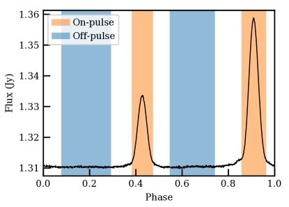
Figure 1: Integrated pulsar profile of PSR B1937+21. The baseband signal at 1 – 1.5 GHz is filtered into 32768 frequency channels and folded into 1024 phase bins. The on-pulse (orange) and off-pulse (blue) ranges are visually selected.

As shown in Fig. 2, there are multiple components in the emission and absorption spectra. In order to measure the radial velocity center and scattering of each H i clouds (clumps of H i gas), it’s necessary to decompose the spectra. Using the $\chi^{2}$ test, we note that 6 Gaussian components together with a constant spectrum baseline are enough to model the observed spectrum. Our fitting model is

$$T_{\mathrm{A}}(f)=A_{0}+\sum_{i=1}^{6}A_{i}e^{-\frac{(f-f_{c,i})^{2}}{2f_{d,i}^{2}}},$$ (2)

where $A_{0}$ is the constant baseline, and $A_{i}$, $f_{c,i}$ and $f_{d,i}$ are the amplitude, center and half width of the $i$-th Gaussian components respectively.

The observed pulsar spectrum is affected by ISM scintillation. As an example, the Arecibo observation of PSR B0540+23 and B2016+28 showed significant scintillation ripples in the pulsar spectra (Stanimirović et al., 2010). In our observation, the broad-band pulsar spectrum is bright around 1420 MHz and fades as the frequency increases. Thus, the H i absorption lines occur on the slope of pulsar spectrum. The scintillation ripples should be carefully removed before measuring absorptive components, otherwise they may generate false structures in the absorption spectra. We use the 1-D spline with explicit internal knots LSQUnivariateSpline in SciPy (Virtanen et al., 2020) to fit for the baseline and interpolate around the absorption lines. For the absorption spectrum, 4 Gaussian components are enough to fit the optical depth, i.e. the optical depth is

$$S/S_{b}=\exp\left[-\sum_{i=1}^{4}A_{i}\exp\left(-\frac{(f-f_{c,i})^{2}}{2f_{d,i}^{2}}\right)\right],$$ (3)

where $S$ is the pulsar spectrum and $S_{b}$ is the baseline.

All the spectral model parameters are inferred with the standard curve-fitting Bayesian method. The sampling of posterior is performed using multiNest (Feroz & Hobson, 2008; Feroz et al., 2009) and pymultiNest (Buchner, 2016). We adopt maximum posterior estimator as the central value of our models.

3.3 H i kinematic distance of the pulsar

The kinematic distance is determined based on the radial velocity of the source and the general revolution of the Milky Way Galaxy. If the source follows the circular orbit of the Galaxy, at a certain direction, its radial velocity depends on its distance according to the Galactic rotation curve. Therefore, by measuring the radial velocity of the source, it’s possible to determine its distance. Following Fich et al. (1989), the observed radial velocity of the source should be

$$v_{r}=R_{0}(\omega-\omega_{0})\sin l\cos b,$$ (4)

where $R_{0}$ is the solar distance to the Galactic center, $l$ and $b$ are the Galactic coordinates of the source, $\omega$ and $\omega_{0}$ are angular velocity of the source and the solar system respectively. Eq. (4) is related to the distances to the Galactic center of the source $R$ and of the Sun $R_{0}$ by

$$\Theta_{0}=\omega R=\omega_{0}R_{0},$$ (5)

and is related to the distance $d$ between them by

$$R^{2}=R_{0}^{2}+d^{2}-2R_{0}d\cos l,$$ (6)

where $\Theta_{0}$ is the circular rotation speed of the Milky Way. Combining Eq. (4)-(6), the kinematic distance of the source is

$$d=R_{0}\left[\cos l\pm\sqrt{\left(1+\frac{v_{r}}{\Theta_{0}\sin l\cos b}\right)^{-2}-\sin^{2}l}\right].$$ (7)

For the outer Galaxy ($\cos l<0$), it’s easy to exclude a negative root. However, for the inner Galaxy ($\cos l>0$), the near and far roots on either sides of the tangent point are possible, which is known as kinematic distance ambiguity (Urquhart et al., 2012).

When applying this method to pulsars, the procedure is complicated due to lack of spectral lines in the pulsar radiation. The observer can only measure the spectral lines of foreground and background clouds to constrain the pulsar distance. For foreground clouds, the observer detects emission line from the clouds and absorption line in the pulsar emission. For background clouds, only emission lines can be detected. Thus the pulsar distance is constrained between the far-most absorptive cloud and the nearest emission-only cloud.

In this work, we adopt the distance to the Galactic center $R_{0}=8.34\,\mathrm{kpc}$ and the circular rotation speed $\Theta_{0}=240\,\mathrm{km\,s^{-1}}$ at the Sun (Reid et al., 2014). The rotation speed is measured in the Local Standard of Rest (LSR), in which the barycentric velocity is $(U,V,W)_{\odot}=(11.1,12.24,7.25)\,\mathrm{km\,s^{-1}}$ defined in Galactic Cartesian velocity components (Schönrich et al., 2010). These updated values are slightly different from the current IAU standard $\Theta_{0}=220\,\mathrm{km\,s^{-1}}$, $R_{0}=8.5\,\mathrm{kpc}$, and $(U,V,W)_{\odot}=(10.0,15.4,7.8)\,\mathrm{km\,s^{-1}}$ (Kerr & Lynden-Bell, 1986). The choice of above galactic model parameters introduce negligible effects comparing to the systematics of kinematic distance method (about $2\,km\,s^{-1}$ in radial velocity and about 1 kpc or less in kinematic distances).

The topocentric frequency of the H i spectrum is first corrected to the barycenter of the solar system. Then the barycentric radial velocity of H i emission and absorption lines are derived from their frequency difference from the reference frequency 1420.4057517667 MHz measured in laboratory (Drake, 2006). The radial velocity in the LSR, $v_{\mathrm{LSR}}$, is then obtained by adding the projection towards the source of $(U,V,W)_{\odot}$. An uncertainty of $\pm 7\,\mathrm{km\,s^{-1}}$ is added to the radial velocity due to the streaming and random motion of the clouds in the Galaxy (Frail & Weisberg, 1990; Weisberg et al., 2008). The kinematic distance of the pulsar is derived from the off-pulse emission spectrum and the on-pulse absorption spectrum. The pulsar distance must be larger than all absorption components’ distances in the on-pulse absorption spectrum, and probably smaller than the distances of the components that only exist in the off-pulse emission spectrum.

3.4 Timing and the anomalous dispersion

We use pulsar timing techniques to measure the pulse time of arrival at each frequency(Lorimer & Kramer, 2005). The timing template is averaged between 1415 and 1425 MHz and smoothed, with the frequencies of the H i line excluded. We implement the Fourier phase gradient algorithm (Taylor, 1992) to time the integrated pulse profiles around the H i absorption line with a Python script.

The timing results is used as independent data to validate our absorption spectrum measurement. As mentioned in Section 3.2, ISM scintillation may generate ripples in the absorption spectra. In addition, Weisberg et al. (1980) and Stanimirović et al. (2010) pointed out that the small number of voltage levels in the digital spectrometer can generate large digitization errors and “ghost” in the spectrum. The noise temperature may also increase significantly due to bright H i emission, which decreases the signal-to-noise ratio (S/N) in the absorption spectrum (Johnston et al., 2003). While the spectral measurement is vulnerable to artifacts due to ISM and instrumental effects, the pulsar timing is less affected. According to the Kramers-Kronig relations (causality of the Green’s function), dispersion must arise when resonance radiation or absorption occurs(Jackson, 1998). The Lorentz dispersion model is a classical model which considers electrons in the medium as the damped harmonic oscillators. In Appendix A, we demonstrate the derivation of the Lorentz dispersion model around the H i spectral line with Gaussian velocity distribution following Jenet et al. (2010), where Eq. (A7) links the dispersion delay $\Delta$ with the optical depth amplitude $\tau_{0}$ and line width $f_{d}$ in the absorption profile. According to Eq. (A7), the anomalous dispersion is sensitive to narrow and deep absorptive features in the spectrum. In this way, we can infer the absorption spectra from the dispersion delay.

4 Results

4.1 Spectral line decomposition & kinematic distance

The off-pulse emission spectrum is decomposed into 6 Gaussian components and a constant baseline as shown in the top panel of Fig. 2. The fitted parameters of the components are presented in Table 1. According to Fig. 2 and 3, and Fig. 3 of Reid et al. (2019), we attribute three emission components (Gaussian 1, 2 and 3 in Table 1) around $v_{\mathrm{LSR}}=-60\,\mathrm{km\,s^{-1}}$ to the Outer Arm of the Milky Way Galaxy, the component around $-5\,\mathrm{km\,s^{-1}}$ (Gaussian 4 in Table 1) to the Perseus Arm, and the component around $35\,\mathrm{km\,s^{-1}}$ (Gaussian 6 in Table 1) to Carina-Sagittarius Arm. The wide Gaussian component 5 in Table 1 may consists of the contribution from the local Orion-Cygnus Arm, Carina-Sagittarius Arm and Perseus Arm.

Table 1: Decomposition of the emission lines. The fitting model is defined in Eq. (2). The frequencies are in the Local Standard of Rest (LSR).

Component	$A$ (K)	$f_{c}$ (MHz)	$f_{d}$ (MHz)
Gaussian 1	$23.5\,^{+6.0}_{-0.6}$	$1420.3234\,^{+0.0050}_{-0.0008}$	$0.03096\,^{+0.00400}_{-0.00014}$
Gaussian 2	$30.10\,^{+0.26}_{-2.20}$	$1420.4028\,^{+0.0120}_{-0.0034}$	$0.0611\,^{+0.0015}_{-0.0090}$
Gaussian 3	$28.3\,^{+2.4}_{-1.7}$	$1420.5099\,^{+0.0007}_{-0.0030}$	$0.0291\,^{+0.0022}_{-0.0010}$
Gaussian 4	$3.7\pm 0.7$	$1420.717\,^{+0.013}_{-0.017}$	$0.095\,^{+0.020}_{-0.006}$
Gaussian 5	$5.3\,^{+1.6}_{-0.9}$	$1420.728\,^{+0.006}_{-0.005}$	$0.0186\,^{+0.0050}_{-0.0030}$
Gaussian 6	$10.8\pm 0.8$	$1420.783\pm 0.004$	$0.0294\,^{+0.0025}_{-0.0040}$
Baseline	$19.865\,^{+0.031}_{-0.100}$

The baseline in the pulsar spectrum is fitted as shown in the second panel of Fig. 2. After removing the baseline due to ISM scintillation, we identify 4 absorption components in the spectrum as shown in the third panel of Fig. 2. We attribute Gaussian components 1 and 2 to the local Orion-Cygnus Arm, and Gaussian components 3 and 4 to Carina-Sagittarius Arm.

Table 2: Decomposition of the absorption lines. The fitting model is defined in Eq. (3). The frequencies are in the Local Standard of Rest (LSR).

Component	$A$	$f_{c}$ (MHz)	$f_{d}$ (MHz)
Gaussian 1	$0.77\,^{+0.09}_{-0.08}$	$1420.3182\,^{+0.0034}_{-0.0025}$	$0.0127\,^{+0.0021}_{-0.0015}$
Gaussian 2	$1.21\,^{+0.09}_{-0.11}$	$1420.3488\,^{+0.0021}_{-0.0017}$	$0.0132\,^{+0.0013}_{-0.0015}$
Gaussian 3	$0.52\pm 0.04$	$1420.4167\,^{+0.0014}_{-0.0013}$	$0.0125\,^{+0.0017}_{-0.0013}$
Gaussian 4	$2.60\pm 0.17$	$1420.4508\pm 0.0006$	$0.0093\pm 0.0004$

The lower bound of the kinematic distance is derived from Gaussian component 4 in Table 2 at $v_{\mathrm{LSR}}\approx 35\,\mathrm{km\,s^{-1}}$. This component is close to the tangent point in Carina-Sagittarius Arm, which is within the $7\,\mathrm{km\,s^{-1}}$ error range due to the streaming and random motion of the clouds. Therefore we adopt the both larger and smaller solutions in Eq. (7) for $-7\,\mathrm{km\,s^{-1}}$ error as the uncertainty of the lower bound of kinematic distance, which is determined at $D_{L}=4.5\pm 2.1\,\mathrm{kpc}$.

The upper bound of the kinematic distance is derived from Gaussian component 4 in Table 1 at $v_{\mathrm{LSR}}\approx-5\,\mathrm{km\,s^{-1}}$, where no absorption line can be identified. Considering $7\,\mathrm{km\,s^{-1}}$ error due to the streaming and random motion of the clouds, the upper bound of the kinematic distance is $D_{U}=9.4\pm 0.5\,\mathrm{kpc}$ according to Eq. (7).

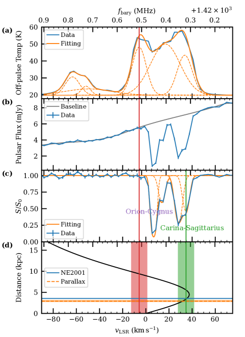
Figure 2: The kinematic distance of PSR B1937+21. The upper x-axis is the barycentric frequency of the spectra. The lower x-axis is the radial velocity in the Local Standard of Rest (LSR). (a) The emission spectrum of antenna temperature at off-pulse phases. The observed spectrum (blue) is fitted with 6 Gaussian components and a constant baseline. The components are plotted with orange dashed curves, and their summation is plotted with the orange solid curve. (b) The absorption spectrum of pulsar emission. The observed spectrum is marked blue. The gray curve shows the fitted baseline. (c) The absorbed fraction. The blue curve is the observed absorption spectrum divided by the baseline in panel (b). The fitted Gaussian components are plotted with orange dashed lines, and the total absorption is plotted with the orange solid line. (d) The radial velocity of Galactic rotation as a function of distance at the direction of PSR B1937+21. The vertical red line denotes the radial velocity of the 4th Gaussian component in the emission spectrum and the red shade denotes its $\pm 7\,\mathrm{km\,m^{-1}}$ error, which determines the upper bound of the kinematic distance in Perseus Arm. The vertical green line denotes the radial velocity of the 4th Gaussian component in the absorption spectrum and the green shade denotes its $\pm 7\,\mathrm{km\,m^{-1}}$ error, which determines the lower bound of the kinematic distance in Carina-Sagittarius Arm. The horizontal blue line is the DM distance estimated using YMW16 model (Yao et al., 2017). The horizontal orange dashed line is the distance calculated from the VLBI parallax (Ding et al., 2023).

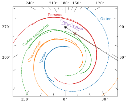
Figure 3: Distance measurement of PSR B1937+21 in the Milky Way Galaxy. The galactic arms are denoted with different colours, viz. Norma-Outer Arm (blue), Crux-Scutum Arm (orange), Carina-Sagittarius Arm (green), Perseus Arm (red) and the local Orion-Cygnus Arm (purple). The solid curves represent the Galactic arm model by Taylor & Cordes (1993), while the dashed curves represents the model by Wainscoat et al. (1992).

4.2 Anomalous dispersion

The lower panel in Fig. 4 exhibit the measured time of arrivals (TOAs) around the H i absorption line in the pulsar emission. At the center of the 4th absorption component, the dispersion delay reaches $-10\,\mathrm{\mu s}$, i.e. the pulse is faster than light by about $10\,\mathrm{\mu s}$. With the Gaussian decomposition of the absorption spectrum in the upper panel of Fig. 4, we derive the theoretical delay curve in the lower panel from Eq. A7, which matches well with the observed TOAs.

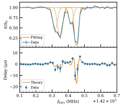
Figure 4: The anomalous dispersion around the H i absorption line in the emission of PSR B1937+21. The upper panel is identical to the panel (c) in Fig. 2. The lower panel shows the dispersion delay of the pulses, in which the blue dots are measured time of arrivals (TOAs), and the orange curve is the theoretical result derived from the absorption spectrum using Eq. A7.

5 Discussion

5.1 A possible tiny-scale atomic structure (TSAS)

PSR B1937+21 is associated with the continuum radio source 4C 21.53W which is a slightly extended H ii region (Sieber & Seiradakis, 1984). In the vicinity, 4C 21.53E (1938+215) is an extragalactic double source (Erickson, 1983). The supernova remnant (SNR) G57.2+0.8 (1932+218) is also known as 4C 21.53 (Ranasinghe et al., 2018; Cotton et al., 2024), which is the host of magnetar SGR J1935+2154 and is not related to PSR B1937+21.

The absorption lines in the pulsar spectra of PSR B1937+21 were previously measured by Heiles et al. (1983) and Jenet et al. (2010) using Arecibo Telescope. The Fig. 1 of Heiles et al. (1983) presented a narrow absorption feature at $-10\,\mathrm{km\,s^{-1}}$ in the absorption spectra towards PSR B1937+21 and 4C 21.53W, which was suspected to be absorbed by a nearby small dust cloud. This narrow absorption line disappeared in the absorption spectrum towards this pulsar in Fig. 2 of Jenet et al. (2010) and in Fig. 2 of this article. We also notice that a wider and shallower component connected the $-10\,\mathrm{km\,s^{-1}}$ component to the $+10\,\mathrm{km\,s^{-1}}$ component in the absorption spectra in Heiles et al. (1983) and Jenet et al. (2010), which is also missing in our result. The comparison of the three absorption spectra is presented in Fig. 5. With the proper motion $0.24\,\mathrm{mas\,yr^{-1}}$ and the distance $D=1/\varpi=1/(0.34\,\mathrm{mas})=2.9\,\mathrm{kpc}$ of PSR B1937+21 (Ding et al., 2023), the variation between 1983 and 2009 corresponds to a spatial structure around 18 AU, and the variation between 2009 and 2020 corresponds to a structure at 8 AU in H i.

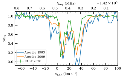
Figure 5: Temporal evolution of H i absorption spectrum towards PSR B1937+21. The blue curve is the Arecibo result extracted from Fig. 1 of Heiles et al. (1983). The orange curve is the Arecibo result extracted from Fig. 3 of Jenet et al. (2010). A velocity offset $-15\,\mathrm{km\,s^{-1}}$ is manually applied to align it with other spectra, because the frequency in Jenet et al. (2010) was topocentric. Data points are digitized using PlotDigitizer (https://plotdigitizer.com/app). The green curve is the result of this article.

Temporal variations of H i absorption profiles towards pulsars have been reported for several pulsars, including PSR B1821+05 (Clifton et al., 1988; Frail et al., 1991), B1557$-$50 (Deshpande et al., 1992; Johnston et al., 2003), and B0301+19 (Weisberg et al., 2008). The variations are attributed to the tiny-scale atomic structures (TSASs) in the ISM (Stanimirović & Zweibel, 2018). The TSAS towards PSR B1937+21 has not been reported in previous literature. This detection provides a new source to monitor the tiny scale fluctuation of H i in the ISM.

However, we must emphasize that the measurement of H i absorption spectrum is vulnerable to possible errors generated during observation and data reduction, as mentioned in Section 3.4. Johnston et al. (2003) pointed out the lack of significance contours manifesting the noise increase due to H i emission in the earlier study by Frail et al. (1994). Weisberg et al. (1980) and Stanimirović et al. (2010) noted that the limited number of voltage levels can generate large digitization errors and “ghost” in the spectrum. We also find that the pulsar spectrum of PSR B1937+21 shows strong scintillation ripples, as also noticed by Stanimirović et al. (2010). Therefore, the baseline removal is crucial in the H i absorption line measurement.

There is also possible variation in other absorption components. In the absorption spectrum in Jenet et al. (2010), the two prominent components at 1420.26 and 1420.37 MHz (topocentric frequency) showed similar amplitude. In our observation, The higher-frequency peak is deeper. The anomalous dispersion presented in Section 4.2 and Fig. 4 may also provide evidence for the possible TSAS. Unlike the spectral line measurement, the digitization error and ISM scintillation should affect the errors of TOAs rather than their expectations. The dispersion delay observed in our observation (lower panel of Fig. 4) is significantly different from Fig. 3 of Jenet et al. (2010), which implies that the absorption spectrum has also changed. Unfortunately, the dispersion delay was not measured in Heiles et al. (1983), and the dispersion is insensitive to the broad component around 1420.45 MHz (topocentric frequency) in Jenet et al. (2010), therefore the previously discussed TSAS around $v_{\mathrm{LSR}}=-5\,\mathrm{km\,s^{-1}}$ cannot be fully assured using anomalous dispersion.

5.2 Update of kinematic distance of PSR B1937+21

The kinematic distance of PSR B1937+21 has been measured in several previous studies. Heiles et al. (1983) acquired the H i emission and absorption spectra of PSR B1937+21 using Arecibo Telescope shortly after its discovery (Backer et al., 1982). Their pulsar spectrum did not show as much as absorption around $v_{r}=40\,\mathrm{km\,s^{-1}}$ as the nearby H ii region 4C 21.53W and extragalactic source 4C 21.53E. They concluded that the pulsar must be closer to us than the tangent point of the spiral arm, and therefore the pulsar distance should be smaller than 5 kpc. In the opposite, Frail & Weisberg (1990) set the lower limit of pulsar distance $D_{L}=4.9\pm 1.9\,\mathrm{kpc}$ at the tangent point, and moved the upper limit to $D_{U}=14.8\pm 0.9\,\mathrm{kpc}$ with the H i emission line around $v_{r}=-60\,\mathrm{km\,s^{-1}}$.

In this manuscript, our lower bound of kinematic distance $D_{L}=4.5\pm 2.1\,\mathrm{kpc}$ is similar to the result of Frail & Weisberg (1990) because we identify the same H i absorption component near the tangent point. However, we shorten the upper bound from $14.8\pm 0.9\,\mathrm{kpc}$ (Frail & Weisberg, 1990) in the Outer Arm to $9.4\pm 0.5\,\mathrm{kpc}$ in the Perseus Arm, because the absorption feature around $v_{\mathrm{LSR}}=-5\,\mathrm{km\,s^{-1}}$ in Heiles et al. (1983) has disappeared in our absorption spectrum. Our result is consistent with the more accurate parallax distance $2.9_{-0.2}^{+0.3}\,\mathrm{kpc}$ (Ding et al., 2023).

5.3 Anomalous dispersion measurement in pulsar observation

Our result confirms the pioneer discovery of apparent faster-than-light dispersion around the H i absorption line Jenet et al. (2010), though the delay curve has changed since 2009 as discussed in Section 5.1. In the lower panel of Fig. 4, the negative delay at the line center implies that the group velocity $v_{\mathrm{g}}$ is greater than the speed of light in vacuum. As discussed in Appendix A, the superluminal group velocity at the center of absorption line can be derived from classical electrodynamics. However, it does not violate causality. The group velocity $v_{\mathrm{g}}=\mathrm{d}\omega/\mathrm{d}k$ is defined as the speed of the Gaussian peak of the wave packet (Jackson, 1998). When radiation or absorption occurs, $v_{\mathrm{g}}$ is no the equivalent to the propagation speed of information (Jenet et al., 2010). The connection between absorption and dispersion, known as Kramers-Kronig relation, is the result of causality in the Green’s function of radio wave propagation in the medium (Jackson, 1998).

According to Eq. (A7), the amplitude of anomalous dispersion depends on both the amplitude and the width of the absorption line. The anomalous dispersion measurement is sensitive to deep and narrow absorption features. However, deep absorption also decreases the observed brightness, which decreases the signal-to-noise ratio (S/N) of the pulse profiles and increases the errors of TOAs. Therefore, the successful measurement of anomalous dispersion in pulsar emission requires dense H i clouds with small velocity dispersion, and bright pulsars in the background. PSR B1937+21 resides near the tangent point, from where the radio wave propagates through a long path in Carina-Sagittarius Arm and the local Orion-Cygnus Arm. The high flux of PSR B1937+21 also increases the precision of timing. We recommend bright millisecond pulsars (MSPs) around tangent points of spiral arms for observations in the future.

Appendix A Anomalous dispersion

In the classical Lorentz dispersion model, the electrons in the medium are considered as damped oscillators stimulated by the electromagnetic wave. In H i clouds, the central frequency of the spectral line is Doppler shifted due to the collective motion of the clouds, and the turbulent and thermal motion inside, which yields the contribution by the hydrogen atoms at multiple velocities. Starting from Eq. (7.51) in Jackson (1998), the dielectric constant, which is also the square of refractive index $n$, should be

$$\epsilon(\omega)=1+\frac{4\pi e^{2}s_{h}}{m_{e}}\int_{0}^{\infty}\frac{n_{h}(\omega^{\prime})}{\omega^{\prime 2}-\omega^{2}-i\omega\gamma}\mathrm{d}\omega^{\prime},$$ (A1)

where $\omega^{\prime}$ is the Doppler shifted frequency of the 21 cm spectral line, $n_{h}(\omega^{\prime})$ is the column density of hydrogen atom at $\omega^{\prime}$, and $s_{h}$ is the oscillator strength of the spectral line. The wave number is $k=\sqrt{\epsilon}\omega/c$, which is known as dispersion relation. Assuming $\epsilon\approx 1$ and $\omega^{\prime 2}-\omega^{2}\approx 2\omega(\omega^{\prime}-\omega)$

$$k\approx\frac{\omega}{c}\left[1+\frac{\pi e^{2}s_{h}}{m_{e}\omega}\int_{0}^{\infty}\frac{n_{h}(\omega^{\prime})}{\omega^{\prime}-\omega-i\gamma/2}\mathrm{d}\omega^{\prime}\right]$$ (A2)

Now we assume that the radial velocity distribution of the H i cloud is Gaussian, i.e. $n_{h}(\omega)=\frac{n_{h,0}}{\sqrt{2\pi}\omega_{d}}\exp\left[-\frac{(\omega-\omega_{c})^{2}}{2\omega_{d}^{2}}\right]$,

$$\int_{-\infty}^{+\infty}\frac{e^{-\frac{(\omega^{\prime}-\omega_{c})^{2}}{2\omega_{d}^{2}}}}{\omega^{\prime}-\omega-i\gamma/2}\mathrm{d}\omega^{\prime}=i\pi\,w\left(\frac{\omega-\omega_{c}+i\gamma/2}{\sqrt{2}\omega_{d}}\right)$$ (A3)

where $w(z)$ is the Faddeeva function $w(z)=\exp(-z^{2})\mathrm{erfc}(-iz)=\frac{i}{\pi}\int_{-\infty}^{+\infty}\frac{e^{-t^{2}}}{z-t}\mathrm{d}t$ (Abramowitz & Stegun, 1972).

After this step, the $\gamma$ term can be negleted because the natural line width is much smaller than the Doppler broading width. The absorption coefficient is

$$\alpha=2\mathrm{Im}(k) \approx\frac{\sqrt{2}\pi^{3/2}e^{2}s_{h}n_{h,0}}{m_{e}c\omega_{d}}\,\mathrm{Re}\,w\left(\frac{\omega-\omega_{c}}{\sqrt{2}\omega_{d}}\right)$$ (A4)

$$=\frac{\sqrt{2}\pi^{3/2}e^{2}s_{h}n_{h,0}}{m_{e}c\omega_{d}}e^{-\frac{(\omega-\omega_{c})^{2}}{2\omega_{d}^{2}}}$$

The group velocity is

$$v_{\mathrm{g}}=\mathrm{Re}\left(\frac{\mathrm{d}\omega}{\mathrm{d}k}\right) \approx c\left[1-\frac{\pi^{3/2}e^{2}s_{h}n_{h,0}}{2m_{e}\omega_{d}^{2}}\,\mathrm{Im}\,w^{\prime}\left(\frac{\omega-\omega_{c}}{\sqrt{2}\omega_{d}}\right)\right]^{-1}$$ (A5)

$$=c\left[1+\frac{\pi^{3/2}e^{2}s_{h}n_{h,0}}{m_{e}\omega_{d}^{2}}\left[\frac{\omega-\omega_{c}}{\sqrt{2}\omega_{d}}e^{-\frac{(\omega-\omega_{c})^{2}}{2\omega_{d}^{2}}}-\frac{1}{\sqrt{\pi}}\right]\right]^{-1}$$

in which $w^{\prime}(z)=-2zw(z)+2i/\sqrt{\pi}$. Assuming the H i cloud is approximately homogeneous, the additional delay due to anomalous dispersion is

$$\Delta=\frac{D}{v_{\mathrm{g}}}-\frac{D}{c}=\frac{D}{c}\frac{\pi^{3/2}e^{2}s_{h}n_{h,0}}{m_{e}\omega_{d}^{2}}\left[\frac{\omega-\omega_{c}}{\sqrt{2}\omega_{d}}e^{-\frac{(\omega-\omega_{c})^{2}}{2\omega_{d}^{2}}}-\frac{1}{\sqrt{\pi}}\right]$$ (A6)

In the same distance, the optical depth of H i absorption is $\tau=\alpha D$ as defined in Eq. (A4).

By fitting the H i absorption line, the amplitude of optical depth $\tau_{0}$, line center frequency $f_{c}$ and line width $f_{d}$ can be obtained as $\tau(f)=\tau_{0}\exp(-(f-f_{c})^{2}/2f_{d}^{2})$, where the angular frequency $\omega$ is converted to frequency $f=\omega/2\pi$. Comparing with Eq. (A4) and (A6), the anomalous dispersion delay is connected with the absorption by

$$\Delta(f)=\frac{\tau_{0}}{2\sqrt{2}\pi f_{d}}\left[\frac{f-f_{c}}{\sqrt{2}f_{d}}e^{-\frac{(f-f_{c})^{2}}{2f_{d}^{2}}}-\frac{1}{\sqrt{\pi}}\right].$$ (A7)

$\Delta(f)$ reaches earliest at the line center where $\Delta_{c}=-\frac{\tau_{0}}{(2\pi)^{3/2}f_{d}}$, which depends on the column density of the H i cloud and the velocity dispersion inside it.

References

- Abramowitz & Stegun (1972) Abramowitz, M., & Stegun, I. A. 1972, Handbook of Mathematical Functions, 297
- Astropy Collaboration et al. (2013) Astropy Collaboration, Robitaille, T. P., Tollerud, E. J., et al. 2013, A&A, 558, A33, doi: 10.1051/0004-6361/201322068
- Astropy Collaboration et al. (2018) Astropy Collaboration, Price-Whelan, A. M., Sipőcz, B. M., et al. 2018, AJ, 156, 123, doi: 10.3847/1538-3881/aabc4f
- Backer et al. (1982) Backer, D. C., Kulkarni, S. R., Heiles, C., Davis, M. M., & Goss, W. M. 1982, Nature, 300, 615, doi: 10.1038/300615a0
- Buchner (2016) Buchner, J. 2016, PyMultiNest: Python interface for MultiNest, Astrophysics Source Code Library, record ascl:1606.005
- Clifton et al. (1988) Clifton, T. R., Frail, D. A., Kulkarni, S. R., & Weisberg, J. M. 1988, ApJ, 333, 332, doi: 10.1086/166749
- Cordes & Lazio (2002) Cordes, J. M., & Lazio, T. J. W. 2002, arXiv e-prints, astro, doi: 10.48550/arXiv.astro-ph/0207156
- Cotton et al. (2024) Cotton, W. D., Kothes, R., Camilo, F., et al. 2024, ApJS, 270, 21, doi: 10.3847/1538-4365/ad0ecb
- Deshpande et al. (1992) Deshpande, A. A., McCulloch, P. M., Radhakrishnan, V., & Anantharamaiah, K. R. 1992, MNRAS, 258, 19P, doi: 10.1093/mnras/258.1.19P
- Dieter et al. (1976) Dieter, N. H., Welch, W. J., & Romney, J. D. 1976, ApJ, 206, L113, doi: 10.1086/182145
- Ding et al. (2023) Ding, H., Deller, A. T., Stappers, B. W., et al. 2023, MNRAS, 519, 4982, doi: 10.1093/mnras/stac3725
- Drake (2006) Drake, G. W. F. 2006, Springer Handbook of Atomic, Molecular, and Optical Physics, 177, doi: 10.1007/978-0-387-26308-3
- Erickson (1983) Erickson, W. C. 1983, ApJ, 264, L13, doi: 10.1086/183936
- Ewen & Purcell (1951) Ewen, H. I., & Purcell, E. M. 1951, Nature, 168, 356, doi: 10.1038/168356a0
- Feroz & Hobson (2008) Feroz, F., & Hobson, M. P. 2008, MNRAS, 384, 449, doi: 10.1111/j.1365-2966.2007.12353.x
- Feroz et al. (2009) Feroz, F., Hobson, M. P., & Bridges, M. 2009, MNRAS, 398, 1601, doi: 10.1111/j.1365-2966.2009.14548.x
- Fich et al. (1989) Fich, M., Blitz, L., & Stark, A. A. 1989, ApJ, 342, 272, doi: 10.1086/167591
- Frail et al. (1991) Frail, D. A., Cordes, J. M., Hankins, T. H., & Weisberg, J. M. 1991, ApJ, 382, 168, doi: 10.1086/170705
- Frail & Weisberg (1990) Frail, D. A., & Weisberg, J. M. 1990, AJ, 100, 743, doi: 10.1086/115556
- Frail et al. (1994) Frail, D. A., Weisberg, J. M., Cordes, J. M., & Mathers, C. 1994, ApJ, 436, 144, doi: 10.1086/174888
- Garrett & McCumber (1970) Garrett, C. G., & McCumber, D. E. 1970, Phys. Rev. A, 1, 305, doi: 10.1103/PhysRevA.1.305
- Gomez-Gonzalez & Guelin (1974) Gomez-Gonzalez, J., & Guelin, M. 1974, A&A, 32, 441
- Graham et al. (1974) Graham, D. A., Mebold, U., Hesse, K. H., Hills, D. L., & Wielebinski, R. 1974, A&A, 37, 405
- Hagen & McClain (1954) Hagen, J. P., & McClain, E. F. 1954, ApJ, 120, 368, doi: 10.1086/145926
- Hagen et al. (1954) Hagen, J. P., McClain, E. F., & Hepburn, N. 1954, AJ, 59, 323, doi: 10.1086/107072
- Harris et al. (2020) Harris, C. R., Millman, K. J., van der Walt, S. J., et al. 2020, Nature, 585, 357, doi: 10.1038/s41586-020-2649-2
- Heiles et al. (1983) Heiles, C., Kulkarni, S. R., Stevens, M. A., et al. 1983, ApJ, 273, L75, doi: 10.1086/184133
- Hobbs et al. (2006) Hobbs, G. B., Edwards, R. T., & Manchester, R. N. 2006, MNRAS, 369, 655, doi: 10.1111/j.1365-2966.2006.10302.x
- Hotan et al. (2004) Hotan, A. W., van Straten, W., & Manchester, R. N. 2004, PASA, 21, 302, doi: 10.1071/AS04022
- Hunter (2007) Hunter, J. D. 2007, Computing in Science and Engineering, 9, 90, doi: 10.1109/MCSE.2007.55
- Jackson (1998) Jackson, J. D. 1998, Classical Electrodynamics, 3rd Edition
- Jenet et al. (2010) Jenet, F. A., Fleckenstein, D., Ford, A., et al. 2010, ApJ, 710, 1718, doi: 10.1088/0004-637X/710/2/1718
- Jiang et al. (2019) Jiang, P., Yue, Y., Gan, H., et al. 2019, Science China Physics, Mechanics, and Astronomy, 62, 959502, doi: 10.1007/s11433-018-9376-1
- Jiang et al. (2020) Jiang, P., Tang, N.-Y., Hou, L.-G., et al. 2020, Research in Astronomy and Astrophysics, 20, 064, doi: 10.1088/1674-4527/20/5/64
- Jing et al. (2023) Jing, W. C., Han, J. L., Hong, T., et al. 2023, MNRAS, 523, 4949, doi: 10.1093/mnras/stad1782
- Johnston et al. (2003) Johnston, S., Koribalski, B., Wilson, W., & Walker, M. 2003, MNRAS, 341, 941, doi: 10.1046/j.1365-8711.2003.06468.x
- Kerr & Lynden-Bell (1986) Kerr, F. J., & Lynden-Bell, D. 1986, MNRAS, 221, 1023, doi: 10.1093/mnras/221.4.1023
- Lorimer & Kramer (2005) Lorimer, D. R., & Kramer, M. 2005, Handbook of pulsar astronomy, Vol. 4 (Cambridge university press)
- Lu et al. (2020) Lu, J., Lee, K., & Xu, R. 2020, Science China Physics, Mechanics, and Astronomy, 63, 229531, doi: 10.1007/s11433-019-1453-2
- Michilli et al. (2018) Michilli, D., Seymour, A., Hessels, J. W. T., et al. 2018, Nature, 553, 182, doi: 10.1038/nature25149
- Minter et al. (2005) Minter, A. H., Balser, D. S., & Kartaltepe, J. S. 2005, ApJ, 631, 376, doi: 10.1086/432367
- Muller & Oort (1951) Muller, C. A., & Oort, J. H. 1951, Nature, 168, 357, doi: 10.1038/168357a0
- Ocker & Cordes (2024) Ocker, S. K., & Cordes, J. M. 2024, Research Notes of the American Astronomical Society, 8, 17, doi: 10.3847/2515-5172/ad1bf1
- Qian et al. (2020) Qian, L., Yao, R., Sun, J., et al. 2020, The Innovation, 1, 100053, doi: 10.1016/j.xinn.2020.100053
- Ranasinghe et al. (2018) Ranasinghe, S., Leahy, D. A., & Tian, W. 2018, Open Physics Journal, 4, 1, doi: 10.2174/1874843001804010001
- Reid et al. (2014) Reid, M. J., Menten, K. M., Brunthaler, A., et al. 2014, ApJ, 783, 130, doi: 10.1088/0004-637X/783/2/130
- Reid et al. (2019) —. 2019, ApJ, 885, 131, doi: 10.3847/1538-4357/ab4a11
- Schönrich et al. (2010) Schönrich, R., Binney, J., & Dehnen, W. 2010, MNRAS, 403, 1829, doi: 10.1111/j.1365-2966.2010.16253.x
- Seymour et al. (2019) Seymour, A., Michilli, D., & Pleunis, Z. 2019, DM_phase: Algorithm for correcting dispersion of radio signals, Astrophysics Source Code Library, record ascl:1910.004
- Sieber & Seiradakis (1984) Sieber, W., & Seiradakis, J. H. 1984, A&A, 130, 257
- Stanimirović et al. (2003) Stanimirović, S., Weisberg, J. M., Hedden, A., Devine, K. E., & Green, J. T. 2003, ApJ, 598, L23, doi: 10.1086/380580
- Stanimirović et al. (2010) Stanimirović, S., Weisberg, J. M., Pei, Z., Tuttle, K., & Green, J. T. 2010, ApJ, 720, 415, doi: 10.1088/0004-637X/720/1/415
- Stanimirović & Zweibel (2018) Stanimirović, S., & Zweibel, E. G. 2018, ARA&A, 56, 489, doi: 10.1146/annurev-astro-081817-051810
- Taylor (1992) Taylor, J. H. 1992, Philosophical Transactions of the Royal Society of London Series A, 341, 117, doi: 10.1098/rsta.1992.0088
- Taylor & Cordes (1993) Taylor, J. H., & Cordes, J. M. 1993, ApJ, 411, 674, doi: 10.1086/172870
- Urquhart et al. (2012) Urquhart, J. S., Hoare, M. G., Lumsden, S. L., et al. 2012, MNRAS, 420, 1656, doi: 10.1111/j.1365-2966.2011.20157.x
- van de Hulst (1945) van de Hulst, H. C. 1945, Nederlandsch Tijdschrift voor Natuurkunde, 11, 210
- van Straten & Bailes (2011) van Straten, W., & Bailes, M. 2011, PASA, 28, 1, doi: 10.1071/AS10021
- Verbiest et al. (2012) Verbiest, J. P. W., Weisberg, J. M., Chael, A. A., Lee, K. J., & Lorimer, D. R. 2012, ApJ, 755, 39, doi: 10.1088/0004-637X/755/1/39
- Virtanen et al. (2020) Virtanen, P., Gommers, R., Oliphant, T. E., et al. 2020, Nature Methods, 17, 261, doi: 10.1038/s41592-019-0686-2
- Wainscoat et al. (1992) Wainscoat, R. J., Cohen, M., Volk, K., Walker, H. J., & Schwartz, D. E. 1992, ApJS, 83, 111, doi: 10.1086/191733
- Weisberg et al. (1980) Weisberg, J. M., Rankin, J., & Boriakoff, V. 1980, A&A, 88, 84
- Weisberg & Stanimirović (2007) Weisberg, J. M., & Stanimirović, S. 2007, in Astronomical Society of the Pacific Conference Series, Vol. 365, SINS - Small Ionized and Neutral Structures in the Diffuse Interstellar Medium, ed. M. Haverkorn & W. M. Goss, 28, doi: 10.48550/arXiv.astro-ph/0701771
- Weisberg et al. (2008) Weisberg, J. M., Stanimirović, S., Xilouris, K., et al. 2008, ApJ, 674, 286, doi: 10.1086/523345
- Williams & Davies (1954) Williams, D. R. W., & Davies, R. D. 1954, Nature, 173, 1182, doi: 10.1038/1731182a0
- Yao et al. (2017) Yao, J. M., Manchester, R. N., & Wang, N. 2017, ApJ, 835, 29, doi: 10.3847/1538-4357/835/1/29