On the Spectral Analysis of Power Graph of Dihedral Groups

Abstract

The power graph $\mathcal{G}_{G}$ of a group $G$ is a graph whose vertex set is $G$, and two elements $x,y\in G$ are adjacent if one is an integral power of the other. In this paper, we determine the adjacency, Laplacian, and signless Laplacian spectra of the power graph of the dihedral group $D_{2pq}$, where $p$ and $q$ are distinct primes. Our findings demonstrate that the results of Romdhini et al. [2024], published in the European Journal of Pure and Applied Mathematics, do not hold universally for all $n\geq 3$. Our analysis demonstrates that their results hold true exclusively when $n=p^{m}$ where $p$ is a prime number and $m$ is a positive integer. The research examines their methodology via explicit counterexamples to expose its boundaries and establish corrected results. This study improves past research by expanding the spectrum evaluation of power graphs linked to dihedral groups.

Keywords: Power Graph, Adjacency Matrix, Laplacian Matrix, Signless Laplacian Matrix, Eigenvalues.
2020 Mathematics Subject Classification: 05C50, 05C25.

1 Introduction

Modern research on studying algebra through graph-theoretic examination has produced diverse intriguing structures that connect algebraic components. The power graph of a group (denoted as $\mathcal{G}_{G}$) represents one of the notable constructions that researchers now focus on intensively. Given a group $G$, the power graph $\mathcal{G}_{G}$ is a graph whose vertex set is $G$, with two distinct vertices $x$ and $y$ being adjacent if and only if one is a power of the other, i.e., $x=y^{k}$ or $y=x^{k}$ for some integer $k$. The dihedral group [16] $D_{2n}$ presents an interesting power graph structure since this is a non-abelian group of order $2n$ consisting of generators $a$ and $b$ where $a$ has order $n$ and $b$ has order $2$ satisfying the relation $ba=a^{-1}b=a^{n-1}b$. The spectral properties of $\mathcal{G}_{D_{2n}}$ enable researchers to understand the graph structure and the underlying group by studying its adjacency spectrum and its Laplacian spectrum and signless Laplacian spectrum.

The adjacency matrix [2] of $\mathcal{G}_{D_{2n}}$, denoted by $A(\mathcal{G}_{D_{2n}})$, is a $2n\times 2n$ matrix whose $(i,j)$-th entry is 1 if the corresponding vertices are adjacent and 0 otherwise. The diagonal degree matrix [2], $D(\mathcal{G}_{D_{2n}})$, is another $2n\times 2n$ matrix where each diagonal entry represents the degree of the corresponding vertex. Laplacian matrices depend heavily on these matrices to establish their definition according to [2] $L(\mathcal{G}_{D_{2n}})=D(\mathcal{G}_{D_{2n}})-A(\mathcal{G}_{D_{2n}})$ and the signless Laplacian matrix [2] $\mathcal{SL}(\mathcal{G}_{D_{2n}})=D(\mathcal{G}_{D_{2n}})+A(\mathcal{G}_{D_{2n}})$ The power graph spectral attributes are discovered through eigenvalue analysis of these matrices that provide knowledge of power graph connectivity status together with classification properties and structural features. The spectrally revealed insights from these matrices lead researchers back to analyze group algebraic properties that exist within the underlying graph structure.

The investigation of power graphs has a rich history. Kelarev and Quinn [9, 10] first introduced the concept of a power graph in the context of semigroups. Subsequent research has explored power graphs in various group settings, including cyclic groups [7, 11], dihedral groups [15], and more general classes of groups. These studies have focused on diverse aspects, such as determining graph-theoretic properties like connectedness, diameter, and clique number, as well as analyzing spectral characteristics. For instance, several studies have characterized the power graphs of specific groups and established relationships between group properties and graph parameters [13, 3]. Sriparna et al. [6] initiated the study of the power graphs of groups in which they investigated the spectral properties of power graphs for cyclic, dihedral, and dicyclic groups. They derive bounds for the spectral radii and partially determine the spectra of these group power graphs. Mehranian et al. in [12] analyzed the spectra of power graphs for various groups, including cyclic, dihedral, elementary abelian groups of prime power order, and the Mathieu group. Their findings offer key spectral insights into the relationship between algebraic and graph-theoretic structures. In [14], various aspects of the Laplacian spectra of power graphs of finite cyclic, dicyclic, and finite $p$-groups have been studied, and the algebraic connectivity has been completely determined for finite $p$-groups. Additionally, in [14], the multiplicity of the Laplacian spectral radius has been analyzed, providing complete results for dicyclic and finite $p$-groups. Also, in [5], the Laplacian spectrum of the power graph of the additive cyclic group $\mathbb{Z}_{n}$ and the dihedral group $D_{n}$ has been studied. It is shown that the Laplacian spectrum of $\mathcal{G}(D_{n})$ is the union of that of $\mathcal{G}(\mathbb{Z}_{n})$ and $\{2n,1\}$. Additionally, the algebraic connectivity of $\mathcal{G}(D_{n})$ is determined, and bounds for the same are provided for $\mathcal{G}(\mathbb{Z}_{n})$. The spectral analysis of power graphs, in particular, has become an active area of research, with investigations into the spectra of power graphs of finite groups leading to interesting connections between algebraic and combinatorial properties. For more on the developments of power graphs of some finite groups, we refer the reader to [11].

Recently, Romdhini et al. [15] published a paper in the European Journal of Pure and Applied Mathematics focusing on the spectral properties of the power graph of dihedral groups, denoted by $D_{2n}$. They presented formulations for the characteristic polynomials of these graphs and claimed their results held generically. However, our analysis reveals that their claimed genericity is not universally valid. This paper critically examines the findings presented in [15]. We demonstrate, through counterexamples, that their main result concerning the characteristic polynomials of the power graph of dihedral groups does not hold for all $n\geq 3$. Specifically, we show that their results are only valid when $n$ is of the form $p^{m}$, where $p$ is a prime number and $m$ is a positive integer. Furthermore, we provide a correction to their result and explicitly calculate the adjacency, Laplacian, and signless Laplacian spectrum of the power graph of $D_{2pq}$ where $p$ and $q$ are distinct primes.

Throughout this paper, we extend the study of power graph spectra by addressing gaps in existing results. Section 2 presents essential definitions and preliminaries. In Section 3, we provide counterexamples to results proved in [15]. Finally, in Section 4, we determine the full adjacency, Laplacian, and signless Laplacian spectrum of $\mathcal{G}_{D_{2pq}}$, further enriching the spectral analysis of power graphs.

2 Preliminaries

This section presents the basic definitions alongside key statements and main theorems which establish our research foundation before introducing our main results. These initial findings derive from existing research studies. This work delivers major insights into spectral and structural properties that were absent from power graphs research before and related algebraic structures. Subsequent theorems and assumptions operate as essential foundations for our exploration. The subsequent sections use these results to build their foundations.

Theorem 2.1.

[4] Let $G$ be a finite group. The $\mathcal{G}_{G}$ is complete if and only if $G$ is either a cyclic group of order $1$ or a cyclic group of order $p^{m}$ for some prime $p$ and for some $m\in\mathbb{N}$.

Theorem 2.2.

[12] Let $G=D_{2n}$ be a dihedral group of order $2n$. Let $n$ be a prime power. Then the characteristic polynomials of both the power graph of the dihedral group $D_{2n}$ can be determined as follows:

$$P(\mathcal{G}(G))=\lambda^{n-1}(\lambda+1)^{n-2}(\lambda^{3}-(n-2)\lambda^{2}-(2n-1)\lambda+n^{2}-2n)$$

Theorem 2.3.

[5] For any non-prime positive integer $n>3$, the Laplacian eigenvalues of $\mathcal{G}_{D_{n}}$ can be expressed in terms of those of $\mathcal{G}_{\mathbb{Z}_{n}}$ as follows:

$$\lambda_{i}(\mathcal{G}_{D_{n}})=\begin{cases}2n,&\text{if }i=1\\ \lambda_{i}(\mathcal{G}_{\mathbb{Z}_{n}})=n,&\text{for }2\leq i\leq\phi(n)+1\\ \lambda_{i}(\mathcal{G}_{\mathbb{Z}_{n}}),&\text{for }\phi(n)+2\leq i\leq n-1\\ 1,&\text{for }n\leq i\leq 2n-1\\ 0,&\text{if }i=2n\end{cases}$$

Theorem 2.4.

[8] Let $A$ be a block upper triangular matrix of the form

$$A=\begin{bmatrix}A_{11}&A_{12}&\cdots&A_{1k}\\ 0&A_{22}&\cdots&A_{2k}\\ \vdots&\vdots&\ddots&\vdots\\ 0&0&\cdots&A_{kk}\end{bmatrix}$$

where each $A_{ii}$ is a square matrix. Then, the determinant of $A$ is given by

$$\det(A)=\det(A_{11})\det(A_{22})\cdots\det(A_{kk}).$$

3 Counterexample and Spectral Properties

The dihedral group $D_{12}=\{\langle a,b\rangle~|~(i)~a^{6}=b^{2}=e~(ii)~ba=a^{-1}b=a^{5}b\}$.

$$\mbox{i.e.,}~D_{12}=\{e,a,a^{2},a^{3},a^{4},a^{5},b,ab,a^{2}b,a^{3}b,a^{4}b,a^{5}b\}.$$

The power graph of the group $D_{12}$ is shown in Figure 1. The eigenvalues for the power graph $D_{12}$ are calculated as follows:

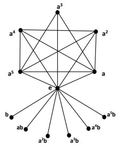
Figure 1: Power graph of $D_{12}$

Example 3.1.

In this example, we have calculated all the adjacency eigenvalues of the power graph $D_{12}$. And then we compared it with the given characteristic polynomial in [15]. We write the adjacency matrix with row and column index by the vertex set $\{e,a,a^{2},a^{3},a^{4},a^{5},b,ab,a^{2}b,a^{3}b,a^{4}b,a^{5}b\}$, making an ordering with partition $\{V_{1},V_{2},V_{3},V_{4},V_{5}\}$. Where $V_{1}=\{e\},V_{2}=\{a,a^{5}\},V_{3}=\{a^{2},a^{4}\},V_{4}=\{a^{4}\},V_{5}=\{b,ab,a^{2}b,a^{3}b,a^{4}b,a^{5}b\}$.

$$A(\mathcal{G}_{D_{12}})=\left[\begin{array}[]{c|c|c|c|c}0&J_{1\times 2}&J_{1\times 2}&J_{1}&J_{1\times 6}\\ \hline\cr J_{2\times 1}&(J-I)_{2}&J_{2}&J_{2\times 1}&O_{2\times 6}\\ \hline\cr J_{2\times 1}&J_{2\times 1}&(J-I)_{2\times 2}&O_{2\times 1}&J_{2\times 6}\\ \hline\cr J_{1}&J_{1\times 2}&O_{1\times 2}&3I_{1}&O_{1\times 6}\\ \hline\cr J_{6\times 1}&O_{6\times 2}&O_{6\times 2}&O_{6\times 1}&O_{6\times 6}\end{array}\right].$$

The eigenvalues of $A(\mathcal{G}_{D_{12}})$ are $0^{(5)},-1^{(2)},-2.924,-1.647,0.356,1.480,4.735.$ But according to the article [15], the characteristic polynomial of $A(\mathcal{G}_{{D}_{12}})$ is $P_{A(\mathcal{G}_{{D}_{12}})}(\lambda)=\lambda^{5}(\lambda+1)^{4}(\lambda^{3}-4\lambda^{2}-11\lambda+24)$. According to this characteristic polynomial, the eigenvalues are $0^{(5)},-1^{(4)},-2.84198,1.61589,5.22609.$ This clearly shows that these are not the eigenvalues of the power graph of the dihedral group ${D}_{12}$.

Example 3.2.

Similarly, for this example, we follow the same vertex ordering and partition as in Example 3.1. Then we calculated all the Laplacian eigenvalues of the power graph $D_{12}$. And then we compared it with the given characteristic polynomial in [15].

$$\mathcal{L}(\mathcal{G}_{D_{12}})=\left[\begin{array}[]{c|c|c|c|c}11&-J_{1\times 2}&-J_{1\times 2}&-J_{1}&-J_{1\times 6}\\ \hline\cr-J_{2\times 1}&(6I-J)_{2}&-J_{2}&-J_{2\times 1}&O_{2\times 6}\\ \hline\cr-J_{2\times 1}&-J_{2\times 1}&(5I-J)_{2\times 2}&O_{2\times 1}&-J_{2\times 6}\\ \hline\cr-J_{1}&-J_{1\times 2}&O_{1\times 2}&(4I-J)_{1}&O_{1\times 6}\\ \hline\cr-J_{6\times 1}&O_{6\times 2}&O_{6\times 2}&O_{6\times 1}&I_{6\times 6}\end{array}\right].$$

The spectrum of $\mathcal{L}(\mathcal{G}_{D_{12}})$ are ${0,1^{(6)},6^{(2)},5,3,12}$. However, the Laplacian characteristic polynomial presented in [15], is $P_{\mathcal{L}(\mathcal{G}_{{D}_{12}})}(\lambda)=\lambda(\lambda-12)(\lambda-6)^{4}(\lambda-1)^{6}$ which is not correct.

Example 3.3.

Similarly, we have calculated all the signless laplacian eigenvalues of the power graph $D_{12}$, by following the same vertex ordering and partition as in Example 3.1. And then we compared it with the given characteristic polynomial in [15].

$$\mathcal{SL}(\mathcal{G}_{D_{12}})=\left[\begin{array}[]{c|c|c|c|c}11&J_{1\times 2}&J_{1\times 2}&J_{1}&J_{1\times 6}\\ \hline\cr J_{2\times 1}&(4I+J)_{2}&J_{2}&J_{2\times 1}&O_{2\times 6}\\ \hline\cr J_{2\times 1}&J_{2\times 1}&(3I+J)_{2\times 2}&O_{2\times 1}&J_{2\times 6}\\ \hline\cr J_{1}&J_{1\times 2}&O_{1\times 2}&(2I+J)_{1}&O_{1\times 6}\\ \hline\cr J_{6\times 1}&O_{6\times 2}&O_{6\times 2}&O_{6\times 1}&I_{6\times 6}\end{array}\right].$$

The characteristic polynomial of the signless Laplacian matrix of $\mathcal{G}_{D_{12}}$ is $P_{\mathcal{SL}(\mathcal{G}_{{D}_{12}})}(\lambda)=(\lambda-1)^{5}(\lambda-4)^{2}(\lambda-3)(\lambda^{4}-22\lambda^{3}+137\lambda^{2}-236\lambda+72)$. But the signless Laplacian characteristic polynomial presented in [15] is $P_{\mathcal{SL}(\mathcal{G}_{{D}_{12}})}(\lambda)=(\lambda-1)^{5}(\lambda-4)^{4}(\lambda-3)(\lambda^{3}-21\lambda^{2}+108\lambda-40)$, which is wrong.

4 Main Results

In this section, we discussed the spectra of power graphs of the dihedral group $D_{2n}$ where $n$ is a product of two distinct primes.

In the following theorem, we provide all the adjacency eigenvalues (or characteristic polynomial) of the power graph of the dihedral group $D_{2pq}$ of order $2pq$, where $p$ and $q$ are distinct primes.

Theorem 4.1.

Consider the dihedral group $G=D_{2pq}$ of order $2pq$, the spectrum of the power graph $\mathcal{G}_{D_{2pq}}$ are $0^{(pq-1)}$, $-1^{(pq-4)}$ and rest of the spectrum are the roots of the equation

$$\lambda^{5}+(4-pq)\lambda^{4}+(7-pq-p-q)\lambda^{3}+M\lambda^{2}+N\lambda+K=0$$

Where $M=2p^{2}q^{2}-2p^{2}q-2pq^{2}+p^{2}+q^{2}-5p-5q+8;~N=2p^{2}q^{2}-p^{2}q+p^{2}-pq^{2}-pq-4p+q^{2}-4q+4;\\ K=2p^{3}q^{2}-p^{3}q^{3}-p^{3}q+2p^{2}q^{3}-4p^{2}q^{2}+3p^{2}q-pq^{3}+3pq^{2}-4pq$

Proof.

It is obvious that the vertex set of the $\mathcal{G}_{D_{2pq}}$ will be $\{e,a,a^{2},...,a^{pq-1},b,ab,a^{2}b,...,a^{pq-1}b\}$. Now, let’s partition these vertices as $\{V_{1},V_{2},V_{3},V_{4},V_{5}\}$ such that $V_{1}$ contains the identity element of $D_{2pq}$ and $V_{2}$ contain all the generators that are $V_{2}=\{a^{i}:\gcd(i,pq)=1\}$ so that $|V_{1}|=1$ and order of $V_{2}=\phi(pq)=(p-1)(q-1)$, also $V_{3}=\{p,2p,...,(q-1)p\}$, $V_{4}=\{q,2q,...,(p-1)q\}$ and $V_{5}=\{b,ab,...,a^{pq-1}b\}$. Then we get the adjacency matrix, in which rows and columns are indexed by the vertex set using the partition $\{V_{1},V_{2},V_{3},V_{4},V_{5}\}$.

$$A(\mathcal{G}_{D_{2pq}})=\begin{bmatrix}O_{1}&J_{1\times\phi(pq)}&J_{1\times(q-1)}&J_{1\times(p-1)}&J_{1\times pq}\\ J_{\phi(pq)\times 1}&(J-I)_{\phi(pq)}&J_{\phi(pq)\times(q-1)}&J_{\phi(pq)\times(p-1)}&O_{\phi(pq)\times pq}\\ J_{(q-1)\times 1}&J_{(q-1)\times\phi(pq)}&(J-I)_{(q-1)}&O_{(q-1)\times(p-1)}&O_{(q-1)\times pq}\\ J_{(p-1)\times 1}&J_{(p-1)\times\phi(pq)}&O_{(p-1)\times(q-1)}&(J-I)_{(p-1)}&O_{(p-1)\times pq}\\ J_{pq\times 1}&O_{pq\times\phi(pq)}&O_{pq\times(q-1)}&O_{pq\times(p-1)}&O_{pq\times pq}\end{bmatrix}$$ (4)

Now, implement the following steps to find the characteristic polynomial of the matrix $A(\mathcal{G}_{D_{2pq}})-\lambda I_{2pq}$.

1. $R_{pq+i}\to R_{pq+i}-R_{pq+1}$ for $2\leq i\leq 2pq$.

2. $C_{pq+1}\to C_{pq+1}+(C_{pq+2}+\cdots+C_{2pq})$.

So the characteristic polynomial (in terms of determinant form) is

$$P_{A(\mathcal{G}_{D_{2pq}})}(\lambda)=\left|\begin{array}[]{ccccccccccc|cccc}-\lambda&1&\cdots&1&1&\cdots&1&1&\cdots&1&pq&1&\cdots&1\\ 1&-\lambda&\cdots&1&1&\cdots&1&1&\cdots&1&0&0&\cdots&0\\ \vdots&\vdots&\ddots&\vdots&\vdots&\ddots&\vdots&\vdots&\ddots&\vdots&\vdots&\vdots&\ddots&\vdots\\ 1&1&\cdots&-\lambda&1&\cdots&1&1&\cdots&1&0&0&\cdots&0\\ 1&1&\cdots&1&-\lambda&\cdots&1&0&\cdots&0&0&0&\cdots&0\\ \vdots&\vdots&\ddots&\vdots&\vdots&\ddots&\vdots&\vdots&\ddots&\vdots&\vdots&\vdots&\ddots&\vdots\\ 1&1&\cdots&1&1&\cdots&-\lambda&0&\cdots&0&0&0&\cdots&0\\ 1&1&\cdots&1&0&\cdots&0&-\lambda&\cdots&1&0&0&\cdots&0\\ \vdots&\vdots&\ddots&\vdots&\vdots&\ddots&\vdots&\vdots&\ddots&\vdots&\vdots&\vdots&\ddots&\vdots\\ 1&1&\cdots&1&0&\cdots&0&1&\cdots&-\lambda&0&0&\cdots&0\\ 1&0&\cdots&0&0&\cdots&0&0&\cdots&0&-\lambda&0&\cdots&0\\ \hline\cr 0&0&\cdots&0&0&\cdots&0&0&\cdots&0&0&-\lambda&\cdots&0\\ \vdots&\vdots&\ddots&\vdots&\vdots&\ddots&\vdots&\vdots&\ddots&\vdots&\vdots&\vdots&\ddots&\vdots\\ 0&0&\cdots&0&0&\cdots&0&0&\cdots&0&0&0&\cdots&-\lambda\\ \end{array}\right|.$$

$=\left|\begin{array}[]{cc}R&Q\\ O&S\end{array}\right|$

Where, $R=\left[\begin{array}[]{ccccccccccc}-\lambda&1&\cdots&1&1&\cdots&1&1&\cdots&1&pq\\ 1&-\lambda&\cdots&1&1&\cdots&1&1&\cdots&1&0\\ \vdots&\vdots&\ddots&\vdots&\vdots&\ddots&\vdots&\vdots&\ddots&\vdots&\vdots\\ 1&1&\cdots&-\lambda&1&\cdots&1&1&\cdots&1&0\\ 1&1&\cdots&1&-\lambda&\cdots&1&0&\cdots&0&0\\ \vdots&\vdots&\ddots&\vdots&\vdots&\ddots&\vdots&\vdots&\ddots&\vdots&\vdots\\ 1&1&\cdots&1&1&\cdots&-\lambda&0&\cdots&0&0\\ 1&1&\cdots&1&0&\cdots&0&-\lambda&\cdots&1&0\\ \vdots&\vdots&\ddots&\vdots&\vdots&\ddots&\vdots&\vdots&\ddots&\vdots&\vdots\\ 1&1&\cdots&1&0&\cdots&0&1&\cdots&-\lambda&0\\ 1&0&\cdots&0&0&\cdots&0&0&\cdots&0&-\lambda\\ \end{array}\right]$, $Q=\left[\begin{array}[]{ccc}1&\cdots&1\\ 0&\cdots&0\\ \vdots&\ddots&\vdots\\ 0&\cdots&0\\ 0&\cdots&0\\ \vdots&\ddots&\vdots\\ 0&\cdots&0\\ 0&\cdots&0\\ \vdots&\ddots&\vdots\\ 0&\cdots&0\\ 0&\cdots&0\\ \end{array}\right]$

$O=\left[\begin{array}[]{ccccccccccc}0&0&\cdots&0&0&\cdots&0&0&\cdots&0&0\\ \vdots&\vdots&\ddots&\vdots&\vdots&\ddots&\vdots&\vdots&\ddots&\vdots&\vdots\\ 0&0&\cdots&0&0&\cdots&0&0&\cdots&0&0\\ \end{array}\right],$ $S=\left[\begin{array}[]{ccc}-\lambda&\cdots&0\\ \vdots&\ddots&\vdots\\ 0&\cdots&-\lambda\\ \end{array}\right]$

By applying Theorem 2.4, we get

$$P_{A(\mathcal{G}_{D_{2pq}})}(\lambda)=\det(R)\det(S)$$

Now, we know that the $\det(S)=(-\lambda)^{pq-1}$. So, to find the characteristic polynomial, we need to solve the determinant of $R$.

Now apply the following steps on $R$

1. $R_{i}\to R_{i}-R_{2}$, $3\leq i\leq\phi(pq)+1$

2. $R_{j}\to R_{j}-R_{\phi(pq)+2}$, $\phi(pq)+3\leq j\leq\phi(pq)+q$

3. $R_{k}\to R_{k}-R_{\phi(pq)+q+1}$, $\phi(pq)+q+2\leq k\leq pq$

After row transformation, we will apply column transformation as

1. $C_{2}\to C_{2}+C_{3}+\cdots+C_{\phi(pq)+1}$

2. $C_{\phi(pq)+2}\to C_{\phi(pq)+2}+C_{\phi(pq)+3}+\cdots+C_{\phi(pq)+q}$

3. $C_{\phi(pq)+q+1}\to C_{\phi(pq)+q+1}+C_{\phi(pq)+q+2}+\cdots+C_{pq}$.

Then we get

$$\det(R)=(\lambda+1)^{pq-4}\begin{vmatrix}-\lambda&(p-1)(q-1)&q-1&p-1&pq\\ 1&(p-1)(q-1)-1-\lambda&q-1&p-1&0\\ 1&(p-1)(q-1)&q-2-\lambda&0&0\\ 1&(p-1)(q-1)&0&(p-2)-\lambda&0\\ 1&0&0&0&-\lambda\end{vmatrix}$$

$$=(\lambda+1)^{pq-4}\{\lambda^{5}+(4-pq)\lambda^{4}+(7-pq-p-q)\lambda^{3}+M\lambda^{2}+N\lambda+K\}$$

Where $M=2p^{2}q^{2}-2p^{2}q-2pq^{2}+p^{2}+q^{2}-5p-5q+8;~N=2p^{2}q^{2}-p^{2}q+p^{2}-pq^{2}-pq-4p+q^{2}-4q+4;\\ K=2p^{3}q^{2}-p^{3}q^{3}-p^{3}q+2p^{2}q^{3}-4p^{2}q^{2}+3p^{2}q-pq^{3}+3pq^{2}-4pq$

Therefore, the characteristic polynomial is

$$P_{A(\mathcal{G}_{D_{2pq}})}(\lambda)=(-\lambda)^{pq-1}(\lambda+1)^{pq-4}\{\lambda^{5}+(4-pq)\lambda^{4}+(7-pq-p-q)\lambda^{3}+M\lambda^{2}+N\lambda+K\}$$

Where $M=2p^{2}q^{2}-2p^{2}q-2pq^{2}+p^{2}+q^{2}-5p-5q+8;~N=2p^{2}q^{2}-p^{2}q+p^{2}-pq^{2}-pq-4p+q^{2}-4q+4;\\ K=2p^{3}q^{2}-p^{3}q^{3}-p^{3}q+2p^{2}q^{3}-4p^{2}q^{2}+3p^{2}q-pq^{3}+3pq^{2}-4pq$

∎

The next theorem provides all the laplacian eigenvalues (or characteristic polynomial) of the power graph of the dihedral group $D_{2pq}$ of order $2pq$, where $p$ and $q$ are distinct primes.

Theorem 4.2.

Let $G=D_{2pq}$ be the dihedral group of order $2pq$, then the spectrum of Laplacian of $\mathcal{G}_{D_{2pq}}$ are

$$0,1^{(pq)},pq^{(\phi(pq))},(pq-p+1)^{(q-2)},(pq-q+1)^{(p-2)},pq-p-q+2,2pq$$

.

Proof.

The construction of the Laplacian matrix of $\mathcal{G}_{D_{2pq}}$ is based on its degree and adjacency matrices. Using the same vertex ordering and partition as in Theorem 4.1, the degree matrix of $\mathcal{G}_{D_{2pq}}$ is

$$\mathcal{D}(\mathcal{G}_{D_{2pq}})=\begin{bmatrix}2pq-1&O_{1\times\phi(pq)}&O_{1\times(q-1)}&O_{1\times(p-1)}&O_{1\times pq}\\ O_{\phi(pq)\times 1}&(pq-1)I_{\phi(pq)}&O_{\phi(pq)\times(q-1)}&O_{\phi(pq)\times(p-1)}&O_{\phi(pq)\times pq}\\ O_{(q-1)\times 1}&O_{(q-1)\times\phi(pq)}&(pq-p)I_{(q-1)}&O_{(q-1)\times(p-1)}&O_{(q-1)\times pq}\\ O_{(p-1)\times 1}&O_{(p-1)\times\phi(pq)}&O_{(p-1)\times(q-1)}&(pq-q)I_{(p-1)}&O_{(p-1)\times pq}\\ O_{pq\times 1}&O_{pq\times\phi(pq)}&O_{pq\times(q-1)}&O_{pq\times(p-1)}&I_{pq\times pq}\end{bmatrix}$$ (6)

From the definition of the Laplacian matrix of $\mathcal{G}(D_{2pq})$, it follows that

$$\mathcal{L}(\mathcal{G}_{D_{2pq}})=\mathcal{D}(\mathcal{G}_{D_{2pq}})-A(\mathcal{G}_{D_{2pq}})$$

where $\mathcal{D}(\mathcal{G}_{D_{2pq}})$ represents the degree matrix and $A(\mathcal{G}_{D_{2pq}})$ denotes the adjacency matrix of $\mathcal{G}_{D_{2pq}}$. Therefore,

$$\mathcal{L}(\mathcal{G}_{D_{2pq}})=\small\begin{bmatrix}2pq-1&-J_{1\times\phi(pq)}&-J_{1\times(q-1)}&-J_{1\times(p-1)}&-J_{1\times pq}\\ -J_{\phi(pq)\times 1}&(pqI-J)_{\phi(pq)}&-J_{\phi(pq)\times(q-1)}&-J_{\phi(pq)\times(p-1)}&O_{\phi(pq)\times pq}\\ -J_{(q-1)\times 1}&-J_{(q-1)\times\phi(pq)}&((pq-p+1)I-J)_{(q-1)}&O_{(q-1)\times(p-1)}&O_{(q-1)\times pq}\\ -J_{(p-1)\times 1}&-J_{(p-1)\times\phi(pq)}&O_{(p-1)\times(q-1)}&((pq-q+1)I-J)_{(p-1)}&O_{(p-1)\times pq}\\ J_{pq\times 1}&O_{pq\times\phi(pq)}&O_{pq\times(q-1)}&O_{pq\times(p-1)}&I_{pq\times pq}\end{bmatrix}.$$

Now, perform the following transformations on the matrix $\mathcal{L}(\mathcal{G}_{D_{2pq}})-\lambda I_{2pq}$, to compute the characteristic polynomial:

1. $R_{pq+i}\to R_{pq+i}-R_{pq+1}$ for $2\leq i\leq 2pq$.

2. $C_{pq+1}\to C_{pq+1}+(C_{pq+2}+\cdots+C_{2pq})$.

After this, we will have a $2\times 2$ block upper triangular matrix (a similar kind of matrix in Theorem 4.1). Again, by applying the row transformation on the 1st block to this Laplacian matrix

1. $R_{i}\to R_{i}-R_{2}$, $3\leq i\leq\phi(pq)+1$

2. $R_{j}\to R_{j}-R_{\phi(pq)+2}$, $\phi(pq)+3\leq j\leq\phi(pq)+q$

3. $R_{k}\to R_{k}-R_{\phi(pq)+q+1}$, $\phi(pq)+q+2\leq k\leq pq$

After this, on applying the column transformation, we have

1. $C_{2}\to C_{2}+C_{3}+\cdots+C_{\phi(pq)+1}$

2. $C_{\phi(pq)+2}\to C_{\phi(pq)+2}+C_{\phi(pq)+3}+\cdots+C_{\phi(pq)+q}$

3. $C_{\phi(pq)+q+1}\to C_{\phi(pq)+q+1}+C_{\phi(pq)+q+2}+\cdots+C_{pq}$

We will get the following:

$$P_{\mathcal{L}(\mathcal{G}_{D_{2pq}})}(\lambda)=(\lambda-1)^{pq-1}(\lambda-(pq-q+1))^{p-2}(\lambda-(pq-p+1))^{q-2}(\lambda-pq)^{\phi(pq)-1}det(B).$$

Where

$$B=\begin{pmatrix}2pq-1-\lambda&-(p-1)(q-1)&1-q&1-p&-pq\\ -1&p+q-1-\lambda&1-q&1-p&0\\ -1&-(p-1)(q-1)&pq-p-q+2-\lambda&0&0\\ -1&-(p-1)(q-1)&0&pq-p-q+2-\lambda&0\\ -1&0&0&0&1-\lambda\end{pmatrix}.$$

Again applying some rows and columns operations, one can get

$$det(M)=(-\lambda)(\lambda-1)(\lambda-pq)(\lambda-pq+p+q-2)(\lambda-2pq).$$

Finally,

$$P_{\mathcal{L}(\mathcal{G}_{D_{2pq}})}(\lambda)=(-\lambda)(\lambda-1)^{pq}(\lambda-pq)^{\phi(pq)}(\lambda-(pq-p+1))^{q-2}(\lambda-(pq-q+1))^{p-2}(\lambda-(pq-p-q+2))(\lambda-2pq).$$

∎

Note 4.1.

The above result can be found in [5] as a corollary of the theorem 2.3. However, our approach is different and more convenient.

Lastly, we provide all the signless Laplacian eigenvalues (or characteristic polynomial) of the power graph of the dihedral group $D_{2pq}$ of order $2pq$, where $p$ and $q$ are distinct primes.

Theorem 4.3.

Let $G=D_{2pq}$ be the dihedral group of order $2pq$, then the spectrum of signless laplacian of $\mathcal{G}_{D_{2pq}}$ are $1^{(pq-1)},(pq-2)^{\phi(pq)},(pq-p-1)^{(q-2)},(pq-q-1)^{(p-2)}$ and the rest of the spectrum are the roots of the biquadratic equation

$$\lambda^{4}-(5pq-p-q-3)\lambda^{3}-X\lambda^{2}-Y\lambda-Z=0$$

Where $X=-8p^{2}q^{2}+4p^{2}q+4pq^{2}+5pq+p+q-4;~Y=4p^{3}q^{3}-4p^{3}q^{2}-4p^{2}q^{3}+4p^{2}q^{2}-2p^{2}q-2pq^{2}-2pq+4p+4q;\\ ~Z=-2p^{3}q^{3}+2p^{3}q^{2}+2p^{2}q^{2}-2p^{2}q-2pq^{2}-4p-4q+8.$

Proof.

From the definition of the Signless Laplacian matrix of $\mathcal{G}_{D_{2pq}}$, it follows that

$$\mathcal{SL}(\mathcal{G}_{D_{2pq}})=\mathcal{D}(\mathcal{G}_{D_{2pq}})+A(\mathcal{G}_{D_{2pq}})$$

where $\mathcal{D}(\mathcal{G}_{D_{2pq}})$ represents the degree matrix and $A(\mathcal{G}_{D_{2pq}})$ denotes the adjacency matrix of $\mathcal{G}_{D_{2pq}}$. Therefore,

$$\mathcal{SL}(\mathcal{G}_{D_{2pq}})=\begin{bmatrix}2pq-1&J_{1\times\phi(pq)}&J_{1\times(q-1)}&J_{1\times(p-1)}&J_{1\times pq}\\ J_{\phi(pq)\times 1}&((pq-2)I+J)_{\phi(pq)}&J_{\phi(pq)\times(q-1)}&J_{\phi(pq)\times(p-1)}&O_{\phi(pq)\times pq}\\ J_{(q-1)\times 1}&J_{(q-1)\times\phi(pq)}&((pq-p-1)I+J)_{(q-1)}&O_{(q-1)\times(p-1)}&O_{(q-1)\times pq}\\ J_{(p-1)\times 1}&J_{(p-1)\times\phi(pq)}&O_{(p-1)\times(q-1)}&((pq-q-1)I+J)_{(p-1)}&O_{(p-1)\times pq}\\ J_{pq\times 1}&O_{pq\times\phi(pq)}&O_{pq\times(q-1)}&O_{pq\times(p-1)}&I_{pq\times pq}\end{bmatrix}$$

Similarly, execute the following operations on the matrix $\mathcal{SL}(\mathcal{G}_{D_{2pq}})-\lambda I_{2pq}$, to compute the characteristic polynomial:

1. $R_{pq+i}\to R_{pq+i}-R_{pq+1}$ for $2\leq i\leq 2pq$.

2. $C_{pq+1}\to C_{pq+1}+(C_{pq+2}+\cdots+C_{2pq})$.

After this, we will have a $2\times 2$ block upper triangular matrix (a similar kind of matrix in Theorem 4.1). Again, the following row transformation on the 1st block is applied to this signless Laplacian matrix.

1. $R_{i}\to R_{i}-R_{2}$, $3\leq i\leq\phi(pq)+1$

2. $R_{j}\to R_{j}-R_{\phi(pq)+2}$, $\phi(pq)+3\leq j\leq\phi(pq)+q$

3. $R_{k}\to R_{k}-R_{\phi(pq)+q+1}$, $\phi(pq)+q+2\leq k\leq pq$

After this, on applying the column transformation, we have

1. $C_{2}\to C_{2}+C_{3}+\cdots+C_{\phi(pq)+1}$

2. $C_{\phi(pq)+2}\to C_{\phi(pq)+2}+C_{\phi(pq)+3}+\cdots+C_{\phi(pq)+q}$

3. $C_{\phi(pq)+q+1}\to C_{\phi(pq)+q+1}+C_{\phi(pq)+q+2}+\cdots+C_{pq}$

We get the following format of the characteristic polynomial:

$$P_{\mathcal{SL}(\mathcal{G}_{D_{2pq}})}(\lambda)=(\lambda-1)^{pq-1}(\lambda-(pq-q-1))^{p-2}(\lambda-(pq-p-1))^{q-2}(\lambda-(pq-2))^{\phi(pq)-1}det(C).$$

Where

$$C=\begin{pmatrix}2pq-1-\lambda&(p-1)(q-1)&q-1&p-1&pq\\ 1&2pq-p-q-1-\lambda&q-1&p-1&0\\ 1&(p-1)(q-1)&pq-p+q-2-\lambda&0&0\\ 1&(p-1)(q-1)&0&pq-q+p-2-\lambda&0\\ 1&0&0&0&1-\lambda\end{pmatrix}.$$

After computing the determinant, we get

$$det(N)=(\lambda-(pq-2))(-\lambda^{4}+(5pq-p-q-3)\lambda^{3}+X\lambda^{2}+Y\lambda+Z).$$

Where $X=-8p^{2}q^{2}+4p^{2}q+4pq^{2}+5pq+p+q-4;~Y=4p^{3}q^{3}-4p^{3}q^{2}-4p^{2}q^{3}+4p^{2}q^{2}-2p^{2}q-2pq^{2}-2pq+4p+4q;\\ ~Z=-2p^{3}q^{3}+2p^{3}q^{2}+2p^{2}q^{2}-2p^{2}q-2pq^{2}-4p-4q+8.$

Therefore,

$$P_{\mathcal{SL}(\mathcal{G}_{D_{2pq}})}(\lambda)=(\lambda-1)^{pq-1}(\lambda-(pq-q-1))^{p-2}(\lambda-(pq-p-1))^{q-2}(\lambda-(pq-2))^{\phi(pq)}(-\lambda^{4}+(5pq-p-q-3)\lambda^{3}+X\lambda^{2}+Y\lambda+Z).$$

Where $X=-8p^{2}q^{2}+4p^{2}q+4pq^{2}+5pq+p+q-4;~Y=4p^{3}q^{3}-4p^{3}q^{2}-4p^{2}q^{3}+4p^{2}q^{2}-2p^{2}q-2pq^{2}-2pq+4p+4q;\\ ~Z=-2p^{3}q^{3}+2p^{3}q^{2}+2p^{2}q^{2}-2p^{2}q-2pq^{2}-4p-4q+8.$

∎

Note 4.2.

One can find the above result in [1], which is a lengthy and complicated proof. Whereas our method is very short and easier.

Declarations

Conflict of interest: There are no conflicts of interest, according to the authors.

References

• [1] Subarsha Banerjee and Avishek Adhikari. On spectra and spectral radius of signless laplacian of power graphs of some finite groups. Asian-european Journal of Mathematics, page 2150090, 2020.
• [2] Andriesย E Brouwer and Willemย H Haemers. Spectra of graphs. Springer Science & Business Media, 2011.
• [3] Peterย J Cameron and Sayyedย Heidar Jafari. On the connectivity and independence number of power graphs of groups. Graphs and Combinatorics, 36(3):895โ€“904, 2020.
• [4] Ivy Chakrabarty, Shamik Ghosh, and MKย Sen. Undirected power graphs of semigroups. In Semigroup Forum, volumeย 78, pages 410โ€“426. Springer, 2009.
• [5] Sriparna Chattopadhyay and Pratima Panigrahi. On laplacian spectrum of power graphs of finite cyclic and dihedral groups. Linear and Multilinear Algebra, 63(7):1345โ€“1355, 2015.
• [6] Sriparna Chattopadhyay, Pratima Panigrahi, and Fouzul Atik. Spectral radius of power graphs on certain finite groups. Indagationes Mathematicae, 29(2):730โ€“737, 2018.
• [7] Sriparna Chattopadhyay, Kamalย Lochan Patra, and Binodย Kumar Sahoo. Vertex connectivity of the power graph of a finite cyclic group. Discrete Applied Mathematics, 266:259โ€“271, 2019.
• [8] Rogerย A Horn and Charlesย R Johnson. Matrix analysis. Cambridge university press, 2012.
• [9] Andreiย V Kelarev and Stephenย J Quinn. A combinatorial property and power graphs of groups. Contributions to general algebra, 12(58):3โ€“6, 2000.
• [10] AVย Kelarev and Sthephenย J Quinn. Directed graphs and combinatorial properties of semigroups. Journal of Algebra, 251(1):16โ€“26, 2002.
• [11] Ajay Kumar, Lavanya Selvaganesh, Peterย J Cameron, and Tย Tamizh Chelvam. Recent developments on the power graph of finite groupsโ€“a survey. AKCE International Journal of Graphs and Combinatorics, 18(2):65โ€“94, 2021.
• [12] Zย Mehranian, Aย Gholami, and ARย Ashrafi. The spectra of power graphs of certain finite groups. Linear and Multilinear Algebra, 65(5):1003โ€“1010, 2017.
• [13] ARย Moghaddamfar, Sย Rahbariyan, and WJย Shi. Certain properties of the power graph associated with a finite group. Journal of Algebra and its Applications, 13(07):1450040, 2014.
• [14] Rameshย Prasad Panda. Laplacian spectra of power graphs of certain finite groups. Graphs and Combinatorics, 35(5):1209โ€“1223, 2019.
• [15] Mamikaย Ujianita Romdhini, Athirah Nawawi, Faisal Al-Sharqi, and Ashraf Al-Quran. Spectral properties of power graph of dihedral groups. European Journal of Pure and Applied Mathematics, 17(2):591โ€“603, 2024.
• [16] Harveyย E Rose. A course on finite groups. Springer Science & Business Media, 2009.