Study of direct and inverse first-exit problems for drifted Brownian motion with Poissonian resetting

Abstract

We address some direct and inverse problems, for the first-exit time (FET) $\tau$ of a drifted Brownian motion with Poissonian resetting ${\cal X}(t)$ from an interval $(0,b)$ and the first-exit area (FEA) $A,$ namely the area swept out by ${\cal X}(t)$ till the time $\tau$; this type of diffusion process ${\cal X}(t)$ is characterized by the fact that a reset to the position $x_{R}$ can occur according to a homogeneous Poisson process with rate $r>0.$ When the initial position ${\cal X}(0)=\eta\in(0,b)$ is deterministic and fixed, the direct FET problem consists in investigating the statistical properties of the FET $\tau,$ whilst the direct FEA problem studies the probability distribution of the FEA $A$. The inverse FET problem regards the case when $\eta$ is randomly distributed in $(0,b)$ (while $r$ and $x_{R}$ are fixed); if $F(t)$ is a given distribution function on the time $t$ axis, the inverse FET problem consists in finding the density $g$ of $\eta,$ if it exists, such that $P[\tau\leq t]=F(t),\ t>0.$ Several explicit examples of solutions to the inverse FET problem are provided.

Keywords: Diffusion with resetting, first-passage time, first-passage place.
Mathematics Subject Classification: 60J60, 60H05, 60H10.

1 Introduction

This paper continues the articles [2] and [3], which respectively concern inverse problems for the first-passage place and the first-passage time, and the first-passage area of a one-dimensional diffusion process $\mathcal{X}(t)$ with Poissonian resetting in an interval $(0,+\infty).$ Here, we address the analogous direct and inverse first-exit time (FET) problems for $\mathcal{X}(t)$ in an interval $(0,b).$ The direct FET problem was also treated in [22], [24], using a slight different approach and a language derived from Physics. In the present paper, our aim is to obtain the quantities of interest as solutions of certain ordinary differential equations with boundary conditions, which in some cases we solve explicitly in terms of elementary functions. As concerns the direct FET problem, for fixed $\mathcal{X}(0)=x\in(0,b)$ we investigate the statistical properties of the FET $\tau(x)$ of $\mathcal{X}(t)$ from the interval $(0,b),$ under the condition that $\mathcal{X}(0)=x,$ that is, $\tau(x)=\min\{t>0:\mathcal{X}(t)\notin(0,b)|\mathcal{X}(0)=x\};$ moreover, we study the probability distribution of the first-exit area (FEA) $A(x),$ namely the area swept out by ${\cal X}(t)$ till the time $\tau(x),$ and the maximum and minimum displacement of ${\cal X}(t)$ for $t\in(0,\tau(x)).$

As for the inverse first-exit time (IFET) problem, we suppose that the starting position $\eta=\mathcal{X}(0)$ is randomly distributed in $(0,b),$ and we denote by $\tau$ the FET of $\mathcal{X}(t)$ from the interval $(0,b);$ then, for a given distribution function $F(t)$ on the the time $t$ axis, the IFET problem consists in finding the probability density $g$ of $\eta,$ if it exists, such that the FET of $\mathcal{X}(t)$ from $(0,b)$ has distribution $F(t),$ namely $P[\tau\leq t]=F(t),\ t>0;$ the density $g$ is called a solution to the IFET problem for $\mathcal{X}(t).$ The analogous IFET problem for diffusions without resetting was studied in [14].

Now, we briefly recall the definition of a one-dimensional diffusion process with Poissonian resetting, $\mathcal{X}(t).$

Let $X(t)$ be a one-dimensional temporally homogeneous diffusion process, driven by the SDE:

$$dX(t)=\mu(X(t))dt+\sigma(X(t))dW_{t},$$ (1.1)

and starting from an initial position $X(0)=\eta\in(0,b)$ (fixed or random), where $W_{t}$ is a standard Brownian motion (BM) and the drift $\mu(\cdot)$ and diffusion coefficient $\sigma(\cdot)$ are regular enough functions, such that there exists a unique strong solution of the SDE (1.1) (see e.g. [27]).

From $X(t)$ we construct a new process ${\cal X}(t),$ as follows. We suppose that resetting events can occur according to a homogeneous Poisson process with rate $r>0.$ Until the first resetting event the process ${\cal X}(t)$ coincides with $X(t)$ and it evolves according to (1.1) with ${\cal X}(0)=X(0)=\eta;$ when the reset occurs, ${\cal X}(t)$ is set instantly to a position $x_{R}\in(0,b).$ After that, ${\cal X}(t)$ evolves again according to (1.1), starting afresh (independently of the past history) from $x_{R},$ until the next resetting event occurs, and so on. The inter-resetting times turn out to be independent and exponentially distributed random variables with parameter $r.$ In other words, in any time interval $(t,t+\Delta t),$ with $\Delta t\rightarrow 0^{+},$ the process can pass from ${\cal X}(t)$ to the position $x_{R}$ with probability $r\Delta t+o(\Delta t),$ or it can continue its evolution according to (1.1) with probability $1-r\Delta t+o(\Delta t).$

The process ${\cal X}(t)$ so obtained is called diffusion process with Poissonian resetting, or more simply diffusion with stochastic resetting; it has some analogies with the process considered in [20], where the authors studied a M/M/1 queue with catastrophes and its continuous approximation, namely a Wiener process subject to randomly occurring jumps at a given rate $\xi,$ each jump making the process instantly obtain the state $0.$ Thus, the process considered in [20] can be viewed as a Wiener process with resetting, in which a reset to the position $x_{R}=0$ is done, according to a homogeneous Poisson process with rate $r=\xi.$

For any $C^{2}$ function $u(x),$ the infinitesimal generator of ${\cal X}(t)$ is given by (see e.g. [3]):

$${\cal L}u(x)=\frac{1}{2}\sigma^{2}(x)u^{\prime\prime}(x)+\mu(x)u^{\prime}(x)+r(u(x_{R})-u(x))\equiv Lu(x)+r(u(x_{R})-u(x)),$$ (1.2)

where $u^{\prime}(x)$ and $u^{\prime\prime}(x)$ stand for the first and second derivative of $u(x).$ Here, $Lu(x)=\frac{1}{2}\sigma^{2}(x)u^{\prime\prime}(x)+\mu(x)u^{\prime}(x)$ represents the “diffusion part” of the generator, i.e. that concerning the diffusion process $X(t).$

Direct and inverse problems for the FET and the FEA of diffusion processes are worthy of attention, since they have interesting applications in several applied fields, for instance in biology in the context of diffusion models for neuronal activity (see e.g. [28], [32] and the references contained in [3]). They are also relevant in Mathematical Finance, in particular in credit risk modeling (see e.g. [25]); other applications can be found e.g. in queuing theory (see e.g. the discussion in [15]); for a review concerning Brownian motion with resetting in physics and computer science, see e.g [31]. For more about inverse passage problems concerning jump-diffusions without resetting, see e.g. [5], [6], [7], [8], [10], [11], [12], [13], [14], [15], [16], [29], [30], [34].

At our knowledge, extensions of inverse FET problems to diffusions with resetting have not been treated in the literature, yet. Thus, the aim of the present article is to study these types of problems for this class of processes, by characterizing the quantities of interest as solutions of suitable ordinary differential equations with boundary conditions.

Of course, one can study FET problems of a diffusion with resetting in any interval $(a,b);$ we have taken $a=0,$ only for the sake of simplicity.

Although we obtain explicit formulae only in the special case when ${\cal X}(t)$ is a drifted Brownian motion with resetting, in principle analogous calculations can be developed for a general one-dimensional diffusion with resetting, whose underlying diffusion is driven by the SDE (1.1). It suffices to replace, in all the differential equations, the generator of drifted Brownian motion, i.e. $Lu(x)=\frac{1}{2}u^{\prime\prime}(x)+\mu u^{\prime}(x),$ with the diffusion part of the generator $\mathcal{L}$ given by (1.2), that is, $Lu(x)=\frac{1}{2}\sigma^{2}(x)u^{\prime\prime}(x)+\mu(x)u^{\prime}(x);$ of course the computations turn out to be more complicated.

The paper is organized as follows. Section 2 treats the direct FET problem when ${\cal X}(t)$ is drifted Brownian motion with resetting: suitable differential problems are stated for the exit probability of ${\cal X}(t)$ from the left end of the interval $(0,b),$ for the Laplace transform and the moments of the FET $\tau(x)$ and the FEA $A(x),$ and for the joint moment of $\tau(x)$ and $A(x);$ finally the probability distributions of the maximum and minimum displacement of ${\cal X}(t)$ till the FET $\tau(x)$ are investigated. In Section 3 the inverse first-exit time (IFET) problem for drifted Brownian motion with resetting is studied and several explicit examples of solutions are provided. Finally, Section 4 contains conclusions and final remarks.

2 The direct first-exit time problem for drifted Brownian motion with resetting

In this Section, $\mathcal{X}(t)$ is drifted Brownian motion with resetting, also called Wiener process with resetting, and we analyze the direct first-exit time problem in $(0,b);$ therefore, we suppose that the underlying diffusion is $X(t)=x+\mu t+W_{t},\ x\in(0,b).$ Then, for any $C^{2}$ function $u(x),$ the infinitesimal generator of ${\cal X}(t)$ is (see (1.2)):

$${\cal L}u(x)=Lu(x)+r(u(x_{R})-u(x))=\frac{1}{2}u^{\prime\prime}(x)+\mu u^{\prime}(x)+r(u(x_{R})-u(x)),$$ (2.1)

where $Lu(x)=\frac{1}{2}u^{\prime\prime}(x)+\mu u^{\prime}(x)$ (we omit to specify the dependence of $L$ and ${\cal L}$ on $\mu,$ for simplicity).

We will find explicit solutions, in terms of elementary functions only, to some differential problems with boundary conditions (see e.g. [2], [3]), concerning the exit probability of $\mathcal{X}(t)$ from the left end of the interval $(0,b),$ and the statistical properties of the FET $\tau_{\mu}(x)$ and the FEA $A_{\mu}(x),$ where

$$\tau_{\mu}(x)=\min\{t>0:\mathcal{X}(t)\notin(0,b)|\mathcal{X}(0)=x\},\ x\in(0,b),$$ (2.2)

denotes the first-exit time (FET) of $\mathcal{X}(t)$ from the interval $(0,b),$ under the condition that $\mathcal{X}(0)=x\in(0,b),$ and

$$A_{\mu}(x)=\int_{0}^{\tau(x)}\mathcal{X}(t)dt$$ (2.3)

is the first-exit area (FEA), i.e. the area swept out by ${\cal X}(t)$ till the time $\tau_{\mu}(x),$ under the condition that $\mathcal{X}(0)=x\in(0,b).$ Moreover, we will study the probability distributions of the maximum and minimum displacement of $\mathcal{X}(t)$ till the FET. For simplicity of notations, we omit to explicit the dependence of all the quantities on $r$ and $x_{R}.$

Since the moments of the FET $\tau_{\mu}(x)$ are finite (this will be shown in Subsection 2.3), then the moments of $A_{\mu}(x)$ are also finite, because $A_{\mu}(x)\leq b\tau_{\mu}(x),$ and so $E[(A_{\mu}(x))^{n}]\leq b^{n}E[(\tau_{\mu}(x))^{n}].$

2.1 The exit probability of $\mathcal{X}(t)$ from the left end of the interval $(0,b)$

From the general theory of jump-diffusion processes with infinitesimal generator $\mathcal{L}$ (see e.g. [16], [21] ) it is known that the exit probability of ${\cal X}(t)$ from the left end of the interval $(0,b),$ when starting from $x\in(0,b),$ that is, $\pi_{0}^{\mu}(x)=P[\mathcal{X}(\tau_{\mu}(x))=0],$ is the solution of the differential problem with boundary conditions:

$$\begin{cases}{\cal L}u(x)=0,\ x\in(0,b)\\ u(0)=1,u(b)=0.\end{cases}$$ (2.4)

Thus, since we consider drifted BM with resetting, the generator ${\cal L}$ is given by (2.1), and so $\pi_{0}^{\mu}(x)$ satisfies:

$$\begin{cases}{\cal L}u(x)=\frac{1}{2}u^{\prime\prime}(x)+\mu u^{\prime}(x)-ru(x)+ru(x_{R})=0,\ x\in(0,b)\\ u(0)=1,u(b)=0.\end{cases}$$ (2.5)

Of course, the exit probability from the right end:

$$\pi_{b}(x)=P[\mathcal{X}(\tau_{\mu}(x))=b]=1-\pi_{0}(x)$$ (2.6)

satisfies the same problem with boundary conditions $u(0)=0,u(b)=1.$ The explicit solution of Eq. (2.5) is (see e.g. Eq. (25) of [22]):

$$\pi_{0}^{\mu}(x)=\frac{\sinh\left((b-x_{R})\sqrt{\mu^{2}+2r}\right)+e^{\mu(b-x)}\sinh\left((x_{R}-x)\sqrt{\mu^{2}+2r}\right)}{\sinh\left((b-x_{R})\sqrt{\mu^{2}+2r}\right)+e^{b\mu}\sinh\left(x_{R}\sqrt{\mu^{2}+2r}\right)},$$ (2.7)

while the probability of exit from the right end of the interval $(0,b)$ is:

$$\pi_{b}^{\mu}(x)=1-\pi_{0}(x)=\frac{e^{b\mu}\sinh\left(x_{R}\sqrt{\mu^{2}+2r}\right)-e^{\mu(b-x)}\sinh\left((x_{R}-x)\sqrt{\mu^{2}+2r}\right)}{\sinh\left((b-x_{R})\sqrt{\mu^{2}+2r}\right)+e^{b\mu}\sinh\left(x_{R}\sqrt{\mu^{2}+2r}\right)}.$$ (2.8)

For $\mu=0,$ one gets the exit probability of (undrifted) BM with resetting:

$$\pi^{0}_{0}(x)=\frac{\sinh((b-x_{R})\sqrt{2r})+\sinh((x_{R}-x)\sqrt{2r}))}{\sinh((b-x_{R})\sqrt{2r})+\sinh(x_{R}\sqrt{2r}))}.$$ (2.9)

If $x=x_{R},$ then:

$$\pi_{0}^{\mu}(x_{R})=\frac{\sinh\left((b-x_{R})\sqrt{\mu^{2}+2r}\right)}{\sinh\left((b-x_{R})\sqrt{\mu^{2}+2r}\right)+e^{b\mu}\sinh\left(x_{R}\sqrt{\mu^{2}+2r}\right)}.$$ (2.10)

Letting $r$ go to infinity in (2.10), one obtains

$$\lim_{r\rightarrow+\infty}\pi_{0}^{\mu}(x)=\begin{cases}1,&x_{R}\in(0,b/2)\\ \frac{1}{1+e^{\mu b}},&x_{R}=b/2\\ 0,&x_{R}\in(b/2,b).\end{cases}$$ (2.11)

Taking the limit as $r\rightarrow 0^{+}$ in (2.7), one gets the well-known result for drifted BM (without resetting), that is (see e.g. [26], pg. 205 or [17], pg. 233):

$$\lim_{r\rightarrow 0^{+}}\pi^{\mu}_{0}(x)=\frac{e^{2(b-x)\mu}-1}{e^{2b\mu}-1},\ x\in(0,b).$$ (2.12)

Finally, letting $\mu$ go to zero in (2.12), one obtains the exit probability of (undrifted) BM without resetting, i.e.

$$\lim_{r\rightarrow 0^{+}}\pi_{0}^{0}(x)=\frac{1}{b}(b-x).$$ (2.13)

Remark 2.1

From (2.7) we can easily obtain the exit probability of $\mathcal{X}(t)$ from the left end of any interval $(a,b),\ a<b,$ under the condition that $\mathcal{X}(0)=x\in(a,b).$ In fact, let $\pi^{-}_{(a,b)}(x;\mu,x_{R},r)$ denote the exit probability from the left end of the interval $(a,b),$ under the condition that $\mathcal{X}(0)=x\in(a,b),$ in particular, with the previous notation it holds $\pi^{-}_{(0,b)}(x;\mu,x_{R},r)=\pi_{0}^{\mu}(x);$ then, it is easy to see that

$$\pi^{-}_{(a,b)}(x;\mu,x_{R},r)=\pi^{-}_{(0,b-a)}(x-a;\mu,x_{R}-a,r).$$ (2.14)

Thus, $\pi^{-}_{(a,b)}(x;\mu,x_{R},r)$ can be obtained from (2.7), by replacing $b$ with $(b-a),\ x$ with $x-a,$ and $x_{R}$ with $x_{R}-a.$

In the Figure 1 we report five examples of the graph of $\pi_{0}^{\mu}(x)$ given by (2.7), as a function of $x\in(0,b),$ for $b=1,\ \mu=1,\ r=1,\ x_{R}=1/4$ (lowest curve); $b=1,\ \mu=1,r=0$ (slightly higher curve); $b=1,\ \mu=0,\ r=0$ (straight line); $b=1,\ \mu=1,\ r=5,\ x_{R}=1/4$ (curve with inflection point);  $b=1,\ \mu=1,\ r=50,\ x_{R}=1/4$ (highest, concave curve). Note that for $r=50$ (large resetting rate), and starting point $x\in(0,1/4),$ the exit probability from the left end of $(0,b)$ is approximately one, in agreement with the theoretical result (2.11).

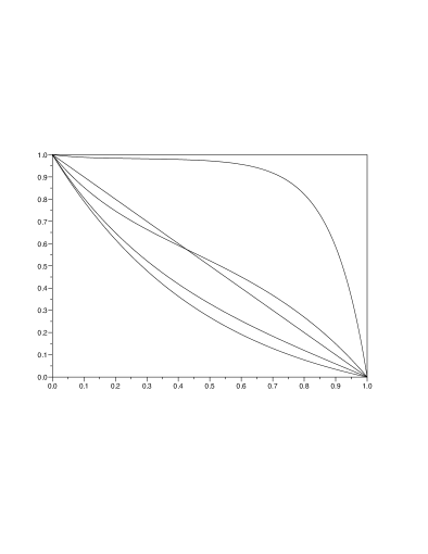
Figure 1: Five examples of the graphs of $\pi_{0}^{\mu}(x)$ given by (2.7), as function of $x\in(0,b),$ for $b=1,\ \mu=1,\ r=1,\ x_{R}=1/4$ (lowest curve); $b=1,\ \mu=1,r=0$ (slightly higher curve); $b=1,\ \mu=0,\ r=0$ (straight line); $b=1,\ \mu=1,\ r=5,\ x_{R}=1/4$ (curve with inflection point);  $b=1,\ \mu=1,\ r=50,\ x_{R}=1/4$ (highest, concave curve).

2.2 The Laplace transforms of the survival function and of the first-exit time

Let $Q^{\mu}_{r}(x,t;x_{R})=P[\tau_{\mu}(x)>t]$ be the survival function of the FET $\tau_{\mu}(x),$ where we use the notation of [22], [24], which makes explicit the dependence on $r$ and $x_{R}.$ Then, $Q^{\mu}_{r}(x,t;x_{R})$ satisfies the backward equation (see e.g. [22], [24]):

$$\frac{\partial}{\partial t}Q^{\mu}_{r}(x,t;x_{R})={\cal L}Q^{\mu}_{r}(x,t;x_{R})$$

$$=\frac{1}{2}\frac{\partial^{2}}{\partial x^{2}}Q^{\mu}_{r}(x,t;x_{R})+\mu\frac{\partial}{\partial x}Q^{\mu}_{r}(x,t;x_{R})+r\left[Q^{\mu}_{r}(x_{R},t;x_{R})-Q^{\mu}_{r}(x,t;x_{R})\right]$$ (2.15)

with the boundary conditions

$$Q^{\mu}_{r}(0,t;x_{R})=Q^{\mu}_{r}(b,t;x_{R})=0,$$ (2.16)

and the initial condition

$$Q^{\mu}_{r}(x,0;x_{R})=1.$$ (2.17)

The operator ${\cal L},$ defined by (2.1), is the infinitesimal generator of drifted BM with resetting $\mathcal{X}(t);$ it is meant as an operator which acts on $Q^{\mu}_{r}(0,t;x_{R}),$ as a function of $x.$ For a general diffusion with resetting, one should take instead the operator given by (1.2).

Note that, by using a renewal argument (see [22]), one obtains:

$$Q^{\mu}_{r}(x,t;x_{R})=e^{-rt}Q^{\mu}_{0}(x,t)+r\int_{0}^{t}dse^{-rs}Q^{\mu}_{0}(x_{R},s)Q^{\mu}_{r}(x,t-s;x_{R}),$$ (2.18)

where $Q^{\mu}_{0}(x,t)$ is the survival function of $\tau_{\mu}(x)$ for the process without resetting, i.e. $r=0.$

For $\lambda>0,$ let $\widehat{Q}^{\mu}_{r}(x,\lambda;x_{R})=\int_{0}^{\infty}e^{-\lambda t}Q^{\mu}_{r}(x,t;x_{R})dt$ be the Laplace transform (LT) of $Q^{\mu}_{r}(x,t;x_{R}),$ and let $\widehat{Q}^{\mu}_{0}(x,\lambda)=\int_{0}^{\infty}e^{-\lambda t}Q^{\mu}_{0}(x,t)dt$ the LT of $Q^{\mu}_{0}(x,t).$ Then from (2.18) one obtains:

$$\widehat{Q}^{\mu}_{r}(x,\lambda;x_{R})=\frac{\widehat{Q}^{\mu}_{0}(x,\lambda+r)}{1-r\widehat{Q}^{\mu}_{0}(x_{R},\lambda+r)}.$$ (2.19)

By taking the Laplace transform in both sides of (2.15), we get that $\widehat{Q}^{\mu}_{r}(x,\lambda;x_{R})$ satisfies, for $\lambda>0,$ the equation:

$$\frac{1}{2}\frac{\partial^{2}}{\partial x^{2}}\widehat{Q}^{\mu}_{r}(x,\lambda;x_{R})+\mu\frac{\partial}{\partial x}Q^{\mu}_{r}(x,\lambda;x_{R})-(r+\lambda)\widehat{Q}^{\mu}_{r}(x,\lambda;x_{R})+r\widehat{Q}^{\mu}_{r}(x_{R},\lambda;x_{R})=-1,$$ (2.20)

subject to the boundary conditions

$$\widehat{Q}^{\mu}_{r}(0,\lambda;x_{R})=\widehat{Q}^{\mu}_{r}(b,\lambda;x_{R})=0.$$ (2.21)

Its explicit solution is (see e.g. Eq. (14) of [22], with $D=1/2):$

$$\widehat{Q}^{\mu}_{r}(x,\lambda;x_{R})=\frac{e^{-b\mu}\sinh(b\beta_{\lambda})-e^{-(b+x)\mu}\sinh(\beta_{\lambda}(b-x))-e^{-\mu x}\sinh(\beta_{\lambda}x)}{\lambda e^{-b\mu}\sinh(\beta_{\lambda}b)+re^{-(b+x_{R})\mu}\sinh(\beta_{\lambda}(b-x_{R}))+re^{-x_{R}\mu}\sinh(\beta_{\lambda}x_{R})},$$ (2.22)

where $\beta_{\lambda}=\sqrt{\mu^{2}+2(\lambda+r)}$ (we omit to explicit the dependence on $\mu$ and $r,$ for simplicity).

We denote by $M_{\mu}(x,\lambda)$ the LT of $\tau_{\mu}(x),$ that is,

$$M_{\mu}(x,\lambda)=E\left[e^{-\lambda\tau(x)}\right]=\int_{0}^{\infty}e^{-\lambda t}f_{\tau_{\mu}}(t)dt,$$

where $f_{\tau_{\mu}}(t)=\frac{d}{dt}P[\tau_{\mu}(x)\leq t]$ is the probability density of $\tau_{\mu}(x)$ (we omit to explicit the dependence of $M_{\mu}(x,\lambda)$ on $r$ and $x_{R}).$ We have:

$$\widehat{Q}^{\mu}_{r}(x,\lambda;x_{R})=\frac{1}{\lambda}\left[1-M_{\mu}(x,\lambda)\right],$$ (2.23)

or

$$M_{\mu}(x,\lambda)=1-\lambda\widehat{Q}^{\mu}_{r}(x,\lambda;x_{R}).$$ (2.24)

In fact:

$$\widehat{Q}^{\mu}_{r}(x,\lambda;x_{R})=\int_{0}^{\infty}e^{-\lambda t}Q^{\mu}_{r}(x,t;x_{R})dt=\int_{0}^{\infty}e^{-\lambda t}\left[1-P(\tau_{\mu}(x)\leq t\right]dt$$

$$=\frac{1}{\lambda}-\int_{0}^{\infty}e^{-\lambda t}P(\tau_{\mu}(x)\leq t)dt.$$ (2.25)

Hence:

$$M_{\mu}(x,\lambda)=\int_{0}^{\infty}e^{-\lambda t}f_{\tau_{\mu}}(t)dt=\int_{0}^{\infty}e^{-\lambda t}\frac{d}{dt}P[\tau_{\mu}(x)\leq t]dt=$$

(integrating by parts)

$$=\lambda\int_{0}^{\infty}e^{-\lambda t}P[\tau_{\mu}(x)\leq t]dt.$$ (2.26)

The last integral is equal to $1/\lambda-\widehat{Q}^{\mu}_{r}(x,\lambda;x_{R}),$ tanking to (2.25); then (2.23) and (2.24) soon follow. By using (2.23), one obtains that $M_{\mu}(x,\lambda),$ as a function of $x,$ satisfies the differential problem (cf. Eq. (2.3) of [3]):

$${\cal L}M_{\mu}(x,\lambda)=\frac{1}{2}\frac{\partial^{2}}{\partial x^{2}}M_{\mu}(x,\lambda)+\mu\frac{\partial}{\partial x}M_{\mu}(x,\lambda)-(r+\lambda)M_{\mu}(x,\lambda)+rM_{\mu}(x_{R},\lambda)=0,\ x\in(0,b)$$ (2.27)

with boundary conditions

$$M_{\mu}(0,\lambda)=M_{\mu}(b,\lambda)=1.$$ (2.28)

From (2.22) the explicit expression of $M_{\mu}(x,\lambda)=1-\lambda\widehat{Q}^{\mu}_{r}(x,\lambda;x_{R})$ soon follows:

$$M_{\mu}(x,\lambda)=1-\frac{\lambda[e^{-b\mu}\sinh(b\beta_{\lambda})-e^{-(b+x)\mu}\sinh(\beta_{\lambda}(b-x))-e^{-\mu x}\sinh(\beta_{\lambda}x)]}{\lambda e^{-b\mu}\sinh(\beta_{\lambda}b)+re^{-(b+x_{R})\mu}\sinh(\beta_{\lambda}(b-x_{R}))+re^{-x_{R}\mu}\sinh(\beta_{\lambda}x_{R})}.$$ (2.29)

In particular:

$$M_{\mu}(x_{R},\lambda)=\frac{(\lambda+r)e^{-\mu x_{R}}\left[\sinh(\beta_{\lambda}x_{R})+e^{-b\mu}\sinh(\beta_{\lambda}(b-x_{R}))\right]}{\lambda e^{-b\mu}\sinh(\beta_{\lambda}b)+re^{-(b+x_{R})\mu}\sinh(\beta_{\lambda}(b-x_{R}))+re^{-x_{R}\mu}\sinh(\beta_{\lambda}x_{R})},$$ (2.30)

that, for $r=0,$ coincides with formula 3.01 of [17], pg. 233.

For $\mu=0,$ one gets from (2.22):

$$\widehat{Q}^{0}_{r}(x,\lambda;x_{R})=\frac{\sinh(\alpha_{\lambda}b)-\sinh(\alpha_{\lambda}x)-\sinh(\alpha_{\lambda}(b-x))}{\lambda\sinh(\alpha_{\lambda}b)+r\sinh(\alpha_{\lambda}x_{R})+r\sinh(\alpha_{\lambda}(b-x_{R}))},$$ (2.31)

and from (2.29):

$$M_{0}(x,\lambda)=\frac{r\sinh(\alpha_{\lambda}x_{R})+r\sinh(\alpha_{\lambda}(b-x_{R}))+\lambda\sinh(\alpha_{\lambda}x)+\lambda\sinh(\alpha_{\lambda}(b-x))]}{\lambda\sinh(\alpha_{\lambda}b)+r\sinh(\alpha_{\lambda}x_{R})+r\sinh(\alpha_{\lambda}(b-x_{R}))},$$ (2.32)

where $\alpha_{\lambda}=\sqrt{2(\lambda+r)}$ (we omit the dependence on $r).$

In particular, for $x=x_{R}:$

$$M_{0}(x_{R},\lambda)=\frac{\left(r+\lambda\right)\left[\sinh(\alpha_{\lambda}x_{R})+\sinh(\alpha_{\lambda}(b-x_{R}))\right]}{\lambda\sinh(\alpha_{\lambda}b)+r\sinh(\alpha_{\lambda}x_{R})+r\sinh(\alpha_{\lambda}(b-x_{R}))}.$$ (2.33)

Letting $b$ go to $+\infty$ in (2.33), one obtains

$$\lim_{b\rightarrow+\infty}M_{0}(x_{R},\lambda)=\frac{(\lambda+r)e^{-x_{R}\sqrt{2(r+\lambda)}}}{\lambda+re^{-x_{R}\sqrt{2(r+\lambda)}}}$$

which coincides with Eq. (3.4) of [3].

For $\mu=r=0,$ namely, for (undrifted) BM without resetting, we obtain

$$\widehat{Q}^{0}_{0}(x,\lambda;x_{R})=\frac{\sinh(\alpha_{\lambda}b)-\sinh(\alpha_{\lambda}x)-\sinh(\alpha_{\lambda}(b-x))}{\lambda\sinh(\alpha_{\lambda}b)},$$ (2.34)

and

$$M_{0}(x,\lambda)=E[e^{-\lambda\tau_{0}(x)}]=1-\lambda\widehat{Q}^{0}_{0}(x,\lambda;x_{R})=\frac{\sinh(\alpha_{\lambda}x)+\sinh(\alpha_{\lambda}(b-x))}{\sinh(\alpha_{\lambda}b)},$$ (2.35)

that, after straightforward algebraic manipulations, coincides with the well-known Darling’s and Siegert’s result [18] (see also [14]):

$$M_{0}(x,\lambda)=E[e^{-\lambda\tau_{0}(x)}]=\frac{\cosh\left(\sqrt{2\lambda}\ (x-\frac{b}{2})\right)}{\cosh\left(\sqrt{2\lambda}\ \frac{b}{2}\right)}.$$ (2.36)

Note that in all cases the LT of the FET, as a function of $\lambda,$ turns out to be well defined and finite even for $\lambda$ belonging to a left neighborhood of $\lambda=0.$ This is also true for $\mu=r=0$ (see (2.36)), as follows by using Euler’s formula. Thus, all the moments of the FET are finite, and therefore also the moments of the FEA are finite.

2.3 The moments of the FET

Since the LT of $\tau_{\mu}(x)$ is finite for $\lambda$ belonging to a neighborhood of $0,$ then the $n-$th order moments of $\tau_{\mu}(x)$ exist finite, and they are given by:

$$T_{n}(x):=E\left[\left(\tau_{\mu}(x)\right)^{n}\right]=(-1)^{n}\left[\frac{\partial^{n}}{\partial\lambda^{n}}M^{\mu}(x,\lambda)\right]_{\lambda=0}\ ,n=1,2,\dots.$$ (2.37)

The moments of $\tau_{\mu}(x)$ can be also obtained from the LT $\widehat{Q}^{\mu}_{r}(x,\lambda;x_{R})$ of the survival function of $\tau_{\mu}(x).$ As easily seen, the first and second moments of $\tau_{\mu}(x)$ are given by:

$$E[\tau(x)]=\widehat{Q}^{\mu}_{r}(x,0;x_{R}),\ \ E[\tau_{\mu}^{2}(x)]=-2\frac{\partial}{\partial\lambda}\widehat{Q}^{\mu}_{r}(x,\lambda;x_{R})|_{\lambda=0}.$$ (2.38)

By setting $T_{0}(x)=1$ and calculating the $n-$th derivative with respect to $\lambda,$ at $\lambda=0,$ of both members of (2.27), we also obtain that the $n-$th order moments $T_{n}(x)$ satisfy the ODEs (see e.g. [2] or [16]):

$$Lu(x)=\frac{1}{2}u^{\prime\prime}(x)+\mu u^{\prime}(x)=-nT_{n-1}(x)+ru(x)-ru(x_{R}),\ x\in(0,b),$$ (2.39)

with the boundary conditions $u(0)=u(b)=0.$ Note that for $r=0$, Eq. (2.39) becomes the celebrated Darling and Siegert’s equation ([18]) for the moments of the first-passage time of a diffusion without resetting.

In particular, $E[\tau_{\mu}(x)]=\widehat{Q}^{\mu}_{r}(x,0;x_{R}),$ as a function of $x,$ is the solution of the differential equation with boundary conditions:

$$\begin{cases}\frac{1}{2}u^{\prime\prime}(x)+\mu u^{\prime}(x)-ru(x)+ru(x_{R})=-1,\ x\in(0.b)\\ u(0)=u(b)=0,\end{cases}$$ (2.40)

whilst $E[\tau_{\mu}^{2}(x)]$ is the solution of the differential problem:

$$\begin{cases}\frac{1}{2}u^{\prime\prime}(x)+\mu u^{\prime}(x)-ru(x)+ru(x_{R})=-2E[\tau(x)],\ x\in(0.b)\\ u(0)=u(b)=0,\end{cases}$$ (2.41)

To obtain the explicit expressions of $E[\tau_{\mu}(x)]$ and $E[\tau_{\mu}^{2}(x)],$ instead of solving (2.40) and (2.41), is more convenient to use formulae (2.38), namely $E[\tau_{\mu}(x)]=\widehat{Q}^{\mu}_{r}(x,0;x_{R}),\ E[\tau_{\mu}^{2}(x)]=-2\frac{\partial}{\partial\lambda}\widehat{Q}^{\mu}_{r}(x,\lambda;x_{R})|_{\lambda=0},$ where $\widehat{Q}^{\mu}_{r}(x,\lambda;x_{R})$ is given by (2.22). Alternatively, $E[\tau_{\mu}(x)]$ and $E[\tau_{\mu}^{2}(x)]$ are respectively given by minus the derivative with respect to $\lambda$ of $M_{\mu}(x,\lambda),$ and its second derivative, both calculated at $\lambda=0.$

In any case, one gets:

$$E[\tau_{\mu}(x)]=$$

$$=\frac{e^{-b\mu}\sinh\left(b\sqrt{\mu^{2}+2r}\ \right)-e^{-\mu x}\sinh\left(x\sqrt{\mu^{2}+2r}\ \right)-e^{-(b+x)\mu}\sinh\left((b-x)\sqrt{\mu^{2}+2r}\ \right)}{r\left[e^{-x_{R}\mu}\sinh\left(x_{R}\sqrt{\mu^{2}+2r}\ \right)+e^{-(b+x_{R})\mu}\sinh\left((b-x_{R})\sqrt{\mu^{2}+2r}\ \right)\right]},$$ (2.42)

The graph of $E[\tau_{\mu}(x)],$ as a function of $x\in(0,b),$ shows a pseudo-parabolic behavior, with the only point of maximum inside the interval $(0,b),$ which is similar to the graph of the expected FET of BM without resetting. In the Figure 2 we report four examples of plots of $E[\tau_{\mu}(x)],$ given by (2.42); the curves are ordered from the lower to the higher peak height. The sets of parameters are: $b=1,\ \mu=1,\ r=0$ (curve 1); $b=1,\ \mu=1,\ r=1,\ x_{R}=1/4$ (curve 2); $b=1,\ \mu=1,\ r=5,\ x_{R}=1/4$ (curve 3); $b=1,\ \mu=0,\ r=0$ (curve 4). Note that for the first three curves the peak is attained approximately at $\bar{x}=0.45,$ while the curve 4, that refers to (undrifted) BM without resetting, attains the maximum exactly at $x=1/2,$ being in this case $E[\tau_{0}(x)]=x(b-x).$

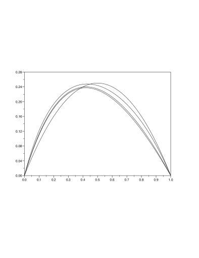
Figure 2: Four examples of plots of $E[\tau_{\mu}(x)],$ as a function of $x\in(0,b);$ the curves are ordered from the lower to the higher peak height. The sets of parameters are: $b=1,\ \mu=1,\ r=0$ (curve 1); $b=1,\ \mu=1,\ r=1,\ x_{R}=1/4$ (curve 2); $b=1,\ \mu=1,\ r=5,\ x_{R}=1/4$ (curve 3); $b=1,\ \mu=0,\ r=0$ (curve 4).

Moreover, it holds:

$$E[\tau_{\mu}^{2}(x)]=$$

$$=\frac{2\left[e^{-\mu b}\sinh(b\beta_{0})-e^{-\mu x}\sinh(x\beta_{0})-e^{-(b+x)\mu}\sinh((b-x)\beta_{0})\right]}{r^{2}\left[e^{-x_{R}\mu}\sinh(x_{R}\beta_{0})+e^{-(b+x_{R})\mu}\sinh((b-x_{R})\beta_{0})\right]^{2}}$$

$$\times\left[e^{-\mu b}\sinh(b\beta_{0})+\frac{r}{\beta_{0}}\left(x_{R}e^{-\mu x_{R}}\cosh(x_{R}\beta_{0})+(b-x_{R})e^{-(b+x_{R})\mu}\cosh(x_{R}\beta_{0})\right)\right]+$$

$$-\frac{2}{\beta_{0}}\ \frac{be^{-\mu b}\cosh(b\beta_{0})-xe^{-\mu x}\cosh(x\beta_{0})-(b-x)e^{-(b+x)\mu}\cosh((b-x)\beta_{0})}{r\left[e^{-x_{R}\mu}\sinh(x_{R}\beta_{0})+e^{-(b+x_{R})\mu}\sinh((b-x_{R})\beta_{0})\right]},$$ (2.43)

where $\beta_{0}=\sqrt{\mu^{2}+2r}.$

Taking the limit as $r\rightarrow 0^{+}$ in (2.42) one obtains the formula for drifted BM without resetting:

$$\lim_{r\rightarrow 0^{+}}E[\tau_{\mu}(x)]=\frac{1}{\mu}\left[\frac{b(1-e^{-2\mu x})}{1-e^{-2\mu b}}-x\right]$$ (2.44)

(in the calculations, it is convenient to use the Taylor’s expansion of $\sinh(\gamma\sqrt{\mu^{2}+2r}),$ as $r\rightarrow 0).$

In the Figure 3 we report four examples of plots of $E[\tau_{\mu}^{2}(x)]$; the curves are ordered from the lower to the higher peak height. The sets of parameters are the same ones as in the Figure 2. Note that for the first three curve the peak is attained approximately at $\bar{x}=0.45,$ while the curve 4, that refers to BM without resetting, attains the maximum exactly at $x=1/2.$

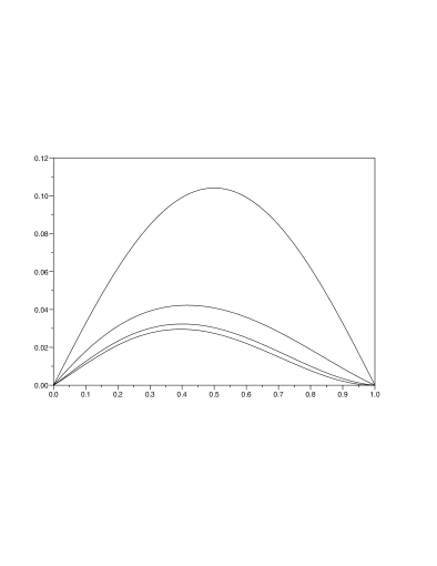
Figure 3: Four examples of plots of $E[\tau_{\mu}^{2}(x)],$ as a function of $x\in(0,b);$ the curves are ordered from the lower to the higher peak height. The sets of parameters are the same ones as in the Figure 2.

For $\mu=0,$ the corresponding expressions for the first two moments of $\tau_{0}(x)$ are the same ones as those with drift, without the exponentials. Note that

$$\max_{x\in(0,b)}E[\tau_{0}(x)]=E[\tau_{0}(b/2)],$$ (2.45)

and, if $x_{R}\notin\{0,b\}:$

$$\lim_{r\rightarrow+\infty}\max_{x\in(0,b)}E[\tau_{0}(x)]=+\infty.$$ (2.46)

For $x=x_{R},$ one obtains:

$$E[\tau_{0}(x_{R})]=\frac{1}{r}\left(\frac{\sinh(b\sqrt{2r})}{\sinh(x_{R}\sqrt{2r})+\sinh((b-x_{R})\sqrt{2r})}-1\right),$$ (2.47)

and letting $b$ go to $+\infty,$ one gets

$$\lim_{b\rightarrow+\infty}E[\tau_{0}(x_{R})]=\frac{1}{r}\left(e^{x_{R}\sqrt{2r}}-1\right),$$ (2.48)

which coincides with Eq. (3.10) of [3], where is treated BM with resetting with $b=+\infty.$

As easily seen (by taking the limit in (2.44) as $\mu\rightarrow 0),$ one finds

$$\lim_{r\rightarrow 0^{+}}E[\tau_{0}(x)]=x(b-x),\ x\in(0,b),$$ (2.49)

that is, the well-known formula for the expected FET of (undrifted) BM without resetting. Moreover, it holds:

$$\lim_{r\rightarrow 0^{+}}E[\tau^{2}_{0}(x)]=\frac{x}{3}[b^{2}(2-b)+bx^{2}(x-2)],\ x\in(0,b),$$ (2.50)

which is the expression of the second moment of the FET of (undrifted) BM without resetting.

2.4 The Laplace transform of the first-exit area

Recall that, for $x\in(0,b),$ the first-exit area (FEA) is:

$$A_{\mu}(x)=\int_{0}^{\tau_{\mu}(x)}{\cal X}(t)dt,\ x\in(0,b).$$ (2.51)

For $\lambda>0,$ let us denote by $N_{\mu}(x,\lambda)$ the LT of $A_{\mu}(x),$ that is,

$$N_{\mu}(x,\lambda)=E\left[e^{-\lambda A_{\mu}(x)}\right].$$ (2.52)

Then, $N_{\mu}(x,\lambda),$ as a function of $x\in(0,b),$ solves the following differential problem with boundary conditions (see e.g. [3], or [12]):

$$\begin{cases}{\cal L}u(x)=\lambda xu(x),\ x\in(0,b)\\ u(0)=u(b)=1,\end{cases}$$ (2.53)

that is,

$$\begin{cases}\frac{1}{2}u^{\prime\prime}(x)+\mu u^{\prime}(x)-\lambda xu(x)-ru(x)+ru(x_{R})=0,\ x\in(0,b)\\ u(0)=u(b)=1.\end{cases}$$ (2.54)

Unfortunately, this is a differential equation with non-constant coefficients and it cannot be solved in terms of elementary functions, but only special functions.

In the special case $\mu=r=0,$ Eq. (2.54) becomes $u^{\prime\prime}(x)-2\lambda xu(x)=0;$ two fundamental solutions are $u_{1}(x)=Ai\left((2\lambda)^{1/3}x\right),$ and $u_{2}(x)=Bi\left((2\lambda)^{1/3}x\right),$ where $Ai$ and $Bi$ are the first and second kind Airy functions (see e.g. [1]). Then, the solution can be written as $u(x)=\alpha_{1}u_{1}(x)+\alpha_{2}u_{2}(x),$ where $\alpha_{1},\alpha_{2}$ are constants with respect to $x$, to be determined (really, they depend on $b$ and $\lambda)$; by imposing the boundary conditions $u(0)=1,u(b)=1,$ one finally finds that the solution of (2.54) is (for $\mu=r=0):$

$$N_{0}(x,\lambda)=\alpha_{1}Ai\left((2\lambda)^{1/3}x\right)+\alpha_{2}Bi\left((2\lambda)^{1/3}x\right),$$ (2.55)

with:

$$\alpha_{1}=\frac{Bi(0)-Bi((2\lambda)^{1/3}b)}{Bi(0)Ai((2\lambda)^{1/3}b)-Bi((2\lambda)^{1/3}b)Ai(0)},\ \alpha_{2}=1-\frac{\alpha_{1}Ai(0)}{Bi(0)}.$$ (2.56)

In the case $b=+\infty,$ the analogous formula for $N_{0}(x,\lambda)$ with $r=0$ was found in [33] (see also [3]).

2.5 The moments of the FEA

Since $\tau_{\mu}(x)$ possesses finite moments of any order $n,$ also the $n-$th order moments of $A_{\mu}(x)$ exist finite, and they are given by:

$$S_{n}(x):=E\left[\left(A_{\mu}(x)\right)^{n}\right]=(-1)^{n}\left[\frac{\partial^{n}}{\partial\lambda^{n}}N_{\mu}(x,\lambda)\right]_{\lambda=0}\ ,n=1,2,\dots.$$ (2.57)

By setting $S_{0}(x)=1$ and calculating the $n-$th derivative with respect to $\lambda,$ at $\lambda=0,$ of both members of Eq. (2.54), we obtains that the $n-$th order moments of $A_{\mu}(x),$ i.e. $S_{n}(x),$ satisfy the ODEs (see e.g. [2] or [12]):

$$LS_{n}(x)=\frac{1}{2}S_{n}^{\prime\prime}(x)+\mu S_{n}^{\prime}(x))-nxS_{n-1}(x)+rS_{n}(x)-rS_{n}(x_{R}),\ x\in(0,b),$$ (2.58)

with the boundary conditions $S_{n}(0)=S_{n}(b)=0.$

Now, we will calculate the first two moments of $A_{\mu}(x).$ Because of complexity of calculations, we will limit ourselves to the case when $\mu=0,$ namely (undrifted) BM with resetting. Note that, for $\mu=0,\ r=0$ (undrifted BM without resetting) and $b=+\infty,$ the moments of $A_{0}(x)$ are infinite (see [9]); instead, for $\mu=0,\ r\geq 0$ and $b<+\infty,$ the moments of $A_{0}(x)$ are finite, because the moments of $\tau_{0}(x)$ are finite.

The Eq. (2.58) for $n=1,$ which provides $E[A_{0}(x)],$ becomes:

$$\begin{cases}\frac{1}{2}u^{\prime\prime}(x)-ru(x)+ru(x_{R})=-x,\ x\in(0,b)\\ u(0)=u(b)=0.\end{cases}$$ (2.59)

By solving it with standard methods, one finds:

$$E[A_{0}(x)]=c_{1}e^{-x\sqrt{2r}}+c_{2}e^{x\sqrt{2r}}+\frac{x}{r}+c_{3},$$ (2.60)

where

$$\begin{cases}c_{1}=\frac{b/r-c_{3}(e^{b\sqrt{2r}}-1)}{2\sinh(b\sqrt{2r})}\\ c_{2}=\frac{-b/r-c_{3}(1-e^{-b\sqrt{2r}})}{2\sinh(b\sqrt{2r})}\\ c_{3}=\frac{1}{r}\ \frac{x_{R}\sinh(b\sqrt{2r})-b\sinh(x_{R}\sqrt{2r})}{\sinh((b-x_{R})\sqrt{2r})+\sinh(x_{R}\sqrt{2r})}\end{cases}$$ (2.61)

(note that the constants $c_{i}$ depend on $b,\ r$ and $x_{R}).$

For $r=0$ Eq. (2.59) simply reads:

$$\begin{cases}\frac{1}{2}u^{\prime\prime}(x)=-x,\ x\in(0,b)\\ u(0)=u(b)=0,\end{cases}$$ (2.62)

whose solution provides:

$$E[A_{0}(x)]=\frac{x}{3}(b^{2}-x^{2})\ (r=0).$$ (2.63)

The second order moment, $E[A_{0}^{2}(x)],$ satisfies the differential problem:

$$\begin{cases}\frac{1}{2}u^{\prime\prime}(x)-ru(x)+ru(x_{R})=-2xE[A_{0}(x)],\ x\in(0,b)\\ u(0)=u(b)=0,\end{cases}$$ (2.64)

whose explicit solution is found by standard methods:

$$E[A_{0}^{2}(x)]=e^{-x\sqrt{2r}}\left[d_{1}+\frac{c_{1}}{\sqrt{2r}}\left(x^{2}+\frac{x}{\sqrt{2r}}\right)\right]+e^{x\sqrt{2r}}\left[d_{2}-\frac{c_{2}}{\sqrt{2r}}\left(x^{2}-\frac{x}{\sqrt{2r}}\right)\right]+$$

$$+\frac{2x^{2}}{r^{2}}+\frac{2c_{3}x}{r}+\frac{2}{r^{3}}+E[A_{0}^{2}(x_{R})],$$ (2.65)

where

$$d_{1}=\Big{\{}e^{-b\sqrt{2r}}\frac{c_{1}}{\sqrt{2r}}\left(b^{2}+\frac{b}{\sqrt{2r}}\right)-e^{b\sqrt{2r}}\frac{c_{2}}{\sqrt{2r}}\left(b^{2}-\frac{b}{\sqrt{2r}}\right)-\frac{2}{r^{3}}\left(e^{b\sqrt{2r}}-1\right)+$$

$$-\left(e^{b\sqrt{2r}}-1\right)E[A_{0}^{2}(x_{R})]+\frac{2b^{2}}{r^{2}}+\frac{2c_{3}b}{r}\Big{\}}\frac{1}{2\sinh(b\sqrt{2r})},$$ (2.66)

$$d_{2}=-\frac{2}{r^{3}}-E[A_{0}^{2}(x_{R})]-d_{1},$$ (2.67)

$$E[A_{0}^{2}(x_{R})]=$$

$$\Big{[}-2d_{1}\sinh(x_{R}\sqrt{2r})+e^{-x_{R}\sqrt{2r}}\frac{c_{1}}{\sqrt{2r}}\left(x_{R}^{2}+\frac{x_{R}}{\sqrt{2r}}\right)-e^{x_{R}\sqrt{2r}}\frac{c_{2}}{\sqrt{2r}}\left(x_{R}^{2}-\frac{x_{R}}{\sqrt{2r}}\right)-\frac{2}{r^{3}}e^{x_{R}\sqrt{2r}}+$$

$$+\frac{2}{r^{2}}x_{R}^{2}+\frac{2c_{3}x_{R}}{r}+\frac{2}{r^{3}}\Big{]}e^{-x_{R}\sqrt{2r}},$$ (2.68)

and finally $c_{i}$ are given by (2.61).

Figure 4: Three examples of graphs of $E[A_{0}(x)],$ as a function of $x\in(0,b);$ the curves are ordered from the higher to the lower peak height. The sets of parameters are: $\mu=0,\ b=1,r=0$ (curve 1); $\mu=0,\ b=1,r=1/2,\ x_{R}=1/8$ (curve 2); $\mu=0,\ b=1,r=5,\ x_{R}=1/8$ (curve 3).

Note that to obtain the solutions to the differential problems (2.59) and (2.64) one has first to solve the associated homogeneous differential equation, and then find a particular solution to be added to the solution of the homogeneous equation. Actually, the calculations to obtain $E[A_{0}(x)]$ and $E[A_{0}^{2}(x)]$ are far more complicated than those necessary to get the corresponding quantities, when $b=+\infty,$ since in that case one of the constants $c_{i}$ and $d_{i}$ vanishes (see [3]). This is the reason why we decided to derive explicit formulae only in the simpler case when $\mu=0$ (undrifted BM with resetting).

In the Figure 4, we report three examples of plots of $E[A_{0}(x)],$ as a function of $x\in(0,b);$ the curves are ordered from the lower to the higher peak height. The sets of parameters are: $\mu=0,\ b=1,r=0$ (curve 1); $\mu=0,\ b=1,r=1/2,\ x_{R}=1/8$ (curve 2); $\mu=0,\ b=1,r=5,\ x_{R}=1/8$ (curve 3). In the Figure 5, we report three examples of plots of $E[A_{0}^{2}(x)],$ as a function of $x\in(0,b);$ the curves are ordered from the lower to the higher peak height, and the sets of parameters are the same ones as in the Figure 4.

Note that for $r=0$ the expression (2.65) for the second moment of $A_{0}(x)$ is not defined, so one has to take the limit as $r$ tends to zero.

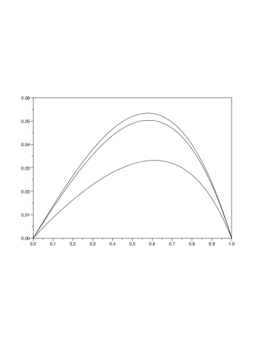
Figure 5: Three examples of graphs of of $E[A^{2}_{0}(x)],$ as a function of $x\in(0,b);$ the curves are from the higher to the lower peak height. The sets of parameters are: $\mu=0,\ b=1,r=0$ (curve 1); $\mu=0,\ b=1,r=1/2,\ x_{R}=1/8$ (curve 2); $\mu=0,\ b=1,r=5,\ x_{R}=1/8$ (curve 3).

2.6 Joint moment of $\tau_{\mu}(x)$ and $A_{\mu}(x)$

This subsection is devoted to find an explicit expression of $E[\tau_{\mu}(x)A_{\mu}(x)],$ i.e. the joint moment of $\tau_{\mu}(x)$ and $A_{\mu}(x).$ Actually, because of complexity of calculations, we will develop the calculations only in the case when $\mu=0.$

The joint LT of $(\tau_{0}(x),A_{0}(x))$ is

$$M_{0}(x,\lambda_{1},\lambda_{2}):=E\left[e^{-\lambda_{1}\tau_{0}(x)}e^{-\lambda_{2}A_{0}(x)}\right],\lambda_{1},\lambda_{2}>0.$$

By reasoning as in [3] or [12], we find that it satisfies the differential equation:

$$(L-r)u(x)=(\lambda_{1}+\lambda_{2}x)u(x)-ru(x_{R}),\ x\in(0,b),$$ (2.69)

with the boundary conditions $u(0)=u(b)=0,$ where now $Lu(x)=\frac{1}{2}u^{\prime\prime}(x),$ because $\mu=0.$

Then, by taking $\frac{\partial^{2}}{\partial\lambda_{1}\partial\lambda_{2}}$ in both members of Eq. (2.69) and calculating it at $\lambda_{1}=\lambda_{2}=0,$ we obtain that the joint moment $V(x):=E[\tau_{0}(x)A_{0}(x)]$ satisfies the boundary value differential problem:

$$\begin{cases}\frac{1}{2}V^{\prime\prime}(x)-rV(x)=-xE[\tau_{0}(x)]-E[A_{0}(x)]-rV(x_{R}),\ x\in(0,b)\\ V(0)=0,\ V(b)=0.\end{cases}$$ (2.70)

Finding its explicit solution is very boring, however, by standard methods, one gets:

$$V(x)=(C_{1}(x)+\beta_{1})e^{-x\sqrt{2r}}+(C_{2}(x)+\beta_{2})e^{x\sqrt{2r}}+V(x_{R}),$$ (2.71)

where the functions $C_{i}(x),\ i=1,2,$ are:

$$C_{1}(x)=\frac{1}{2\sqrt{2r}}\Big{\{}e^{x\sqrt{2r}}\left[\left(\frac{x}{\sqrt{2r}}-\frac{1}{2r}\right)\left(\frac{D_{2}}{D_{1}}+\frac{1}{r}\right)+\frac{c_{3}}{\sqrt{2r}}\right]$$

$$+\frac{1-e^{b\sqrt{2r}}}{4D_{1}}x^{2}+c_{1}x+e^{2x\sqrt{2r}}\left[\frac{e^{-b\sqrt{2r}}-1}{8D_{1}}\left(\frac{2x}{\sqrt{2r}}-\frac{1}{2r}\right)+\frac{c_{2}}{2\sqrt{2r}}\right]\Big{\}}$$ (2.72)

$$C_{2}(x)=\frac{1}{2\sqrt{2r}}\Big{\{}e^{-x\sqrt{2r}}\left[\left(\frac{x}{\sqrt{2r}}+\frac{1}{2r}\right)\left(\frac{D_{2}}{D_{1}}+\frac{1}{r}\right)+\frac{c_{3}}{\sqrt{2r}}\right]+$$

$$+\frac{1-e^{-b\sqrt{2r}}}{4D_{1}}x^{2}-c_{2}x+e^{-2x\sqrt{2r}}\left[\frac{1-e^{b\sqrt{2r}}}{2D_{1}}\left(\frac{x}{2\sqrt{2r}}+\frac{1}{8r}\right)+\frac{c_{1}}{2\sqrt{2r}}\right]\Big{\}},$$ (2.73)

with:

$$D_{1}=r[\sinh(x_{R}\sqrt{2r})+\sinh((b-x_{R})\sqrt{2r})],\ D_{2}=\sinh(b\sqrt{2r}),$$ (2.74)

and $c_{1},\ c_{2},\ c_{3}$ are given by (2.61) (we omit the dependence of the functions $C_{i}(x)$ and the constants $D_{i}$ on $b,r,x_{R}).$ By imposing the boundary conditions $V(0)=0,\ V(b)=0,$ one finds the constants $\beta_{i}$ (actually, they depend on $b,r,x_{R}):$

$$\beta_{1}=-\frac{V(x_{R})(e^{b\sqrt{2r}}-1)-C_{1}(b)e^{-b\sqrt{2r}}-\left[C_{2}(b)-C_{1}(0)-C_{2}(0)\right]e^{b\sqrt{2r}}}{2\sinh(b\sqrt{2r})}$$ (2.75)

$$\beta_{2}=-V(x_{R})-C_{1}(0)-C_{2}(0)-\beta_{1}.$$ (2.76)

Finally, by taking $x=x_{R}$ in (2.71), one obtains an equation in the unknown $V(x_{R}),$ which allows to find it:

$$V(x_{R})=\Big{\{}C_{1}(x_{R})e^{-2x_{R}\sqrt{2r}}+C_{2}(x_{R})-C_{1}(b)\ \frac{\sinh(x_{R}\sqrt{2r})}{\sinh(b\sqrt{2r})}\ e^{-(x_{R}+b)\sqrt{2r}}+$$

$$-\frac{\sinh(x_{R}\sqrt{2r})}{\sinh(b\sqrt{2r})}\ e^{(b-x_{R})\sqrt{2r}}\ \Big{[}C_{2}(b)-C_{1}(0)-C_{2}(0)\Big{]}-C_{1}(0)-C_{2}(0)\Big{\}}$$

$$\times\Big{\{}1-\frac{\sinh(x_{R}\sqrt{2r})}{\sinh(b\sqrt{2r})}\left(e^{b\sqrt{2r}}-1\right)e^{-x_{R}\sqrt{2r}}\ \Big{\}}^{-1}$$ (2.77)

(note that the expression in $\{\ \}$ is positive for every value of $x_{R}).$

Thus, the explicit forms of $E[\tau_{0}(x)A_{0}(x)]=V(x)$ and of $Cov[\tau_{0}(x),A_{0}(x)]=E[\tau_{0}(x)A_{0}(x)]-E[\tau_{0}(x)]E[A_{0}(x)]$ is obtained from (2.71), (2.42) with $\mu=0,$ and (2.60).

In the Figure 6, we report an example of the graph of $E[\tau_{0}(x_{R})A_{0}(x_{R})]$ (left panel) and the graph of $Cov[\tau_{0}(x_{R}),A_{0}(x_{R})]$ (right panel), as functions of $x_{R}\in(0,b),$ for $b=1$ and $r=1/2.$ As we see, $Cov[\tau_{0}(x_{R}),A_{0}(x_{R})]$ is positive, that is $\tau_{0}(x_{R})$ and $A_{0}(x_{R})$ are positively correlated; the covariance starts from zero, it reaches its maximum in the interior of $(0,b),$ and then it vanishes at $x_{R}=b$ again (compare this behavior with that of $Cov[\tau_{0}(x),A_{0}(x)]$ in the case of BM with resetting with $b=+\infty,$ see [3]).

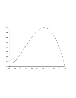
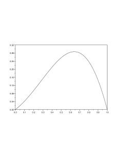
Figure 6: Graphs of $E[\tau_{0}(x_{R})A_{0}(x_{R})]$ (left panel) and $Cov[\tau_{0}(x_{R}),A_{0}(x_{R})]$ (right panel), as functions of $x_{R}\in(0,b),$ in the case of BM with resetting, for $b=1,r=1/2.$

2.7 The distributions of the maximum and minimum displacement till the exit time

The maximum displacement of ${\cal X}(t),$ starting from $x\in(0,b),$ till the FET $\tau_{\mu}(x)$, is the r.v. $\mathcal{M}_{x}=\max_{t\in[0,\tau_{\mu}(x)]}{\cal X}(t)$ (of course one has $b\geq\mathcal{M}_{x}\geq x).$ Two cases are possible: in the first one ${\cal X}(t)$ first exits the interval $(0,b)$ through $0,$ and one can only say that $\mathcal{M}_{x}\geq x,$ in the second case ${\cal X}(t)$ first exits the interval $(0,b)$ through $b$ and $\mathcal{M}_{x}=b.$ Let us denote by $E_{0}$ and $E_{b},$ the event that ${\cal X}(t)$ first exits the interval $(0,b)$ through $0,$ respectively $b,$ namely $E_{0}=\{\mathcal{X}(\tau_{\mu}(x))=0\},\ E_{b}=\{\mathcal{X}(\tau_{\mu}(x))=b\}.$ For $b\geq z\geq x,$ the event $\{\mathcal{M}_{x}\leq z,\ \mathcal{X}(\tau_{\mu}(x))=0\}$ occurs if and only if ${\cal X}(t)$ first exits the interval $(0,z)$ through the left end $0.$ Therefore, for $b\geq z\geq x$ one gets that $w_{\mathcal{M}}(z):=P(\mathcal{M}_{x}\leq z,\ {\cal X}(\tau_{\mu}(x))=0)$ is the solution of the differential boundary problem (see [3], [12]):

$$\begin{cases}Lu(x)+ru(x_{R})-ru(x)=0,\ x\in(0,z)\\ u(0)=1,\ u(z)=0,\end{cases}$$ (2.78)

with $Lu=\frac{1}{2}u^{\prime\prime}(x)+\mu u^{\prime}(x).$

Its explicit form is obtained from (2.7), by replacing the interval $(0,b)$ with $(0,z),$ so obtaining:

$$P\left[\mathcal{M}_{x}\leq z,{\cal X}(\tau_{\mu}(x))\right]=0)=\begin{cases}0,&z<x\\ \frac{\sinh\left((z-x_{R})\sqrt{\mu^{2}+2r}\right)+e^{\mu(z-x)}\sinh\left((x_{R}-x)\sqrt{\mu^{2}+2r}\right)}{\sinh\left((z-x_{R})\sqrt{\mu^{2}+2r}\right)+e^{z\mu}\sinh\left(x_{R}\sqrt{\mu^{2}+2r}\right)},&x\leq z\leq b.\end{cases}$$ (2.79)

Thus $w_{\mathcal{M}}(z)$ increases from $0$ to $\pi^{\mu}_{0}(x).$

The conditional distribution function of $\mathcal{M}_{x}$ is:

$$F_{\mathcal{M}_{x}|E_{0}}(z)=\frac{P[\mathcal{M}_{x}\leq z,{\cal X}(\tau_{\mu}(x))=0]}{\pi^{\mu}_{0}(x)}=\frac{w_{\mathcal{M}}(z)}{\pi^{\mu}_{0}(x)}.$$ (2.80)

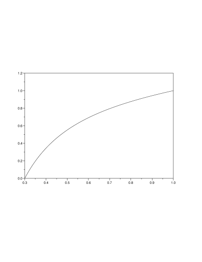
Figure 7: An example of the graph of the conditional distribution of $\mathcal{M}_{x},$ given by (2.80), as a function of $z\in(x,b),$ for $b=1,\ \mu=1,\ r=1,\ x_{R}=1/4$ and $x=0.3\ .$

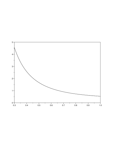
Figure 8: An example of the graph of the conditional density of $\mathcal{M}_{x}$ given by (2.82), as a function of $z\in(x,b),$ for $b=1,\ \mu=1,\ r=1,\ x_{R}=x=0.3\ .$

For instance, if $x=x_{R},$ (2.79) becomes:

$$P\left[\mathcal{M}_{x}\leq z,{\cal X}(\tau_{\mu}(x))=0\right]=\frac{\sinh\left((z-x_{R})\sqrt{\mu^{2}+2r}\right)}{\sinh\left((z-x_{R})\sqrt{\mu^{2}+2r}\right)+e^{z\mu}\sinh\left(x_{R}\sqrt{2r}\right)},$$ (2.81)

and (see also Eq. (28) of [22]):

$$\frac{d}{dz}P\left[\mathcal{M}_{x}\leq z,{\cal X}(\tau_{\mu}(x))=0\right]=$$

$$=\begin{cases}0&\ \ z<x\\ \frac{e^{z\mu}\sinh\left(x\sqrt{\mu^{2}+2r}\right)\left[\sqrt{\mu^{2}+2r}\cosh\left((z-x)\sqrt{\mu^{2}+2r}\right)-\mu\sinh\left((z-x)\sqrt{\mu^{2}+2r}\right)\right]}{\left[\sinh((z-x)\sqrt{\mu^{2}+2r})+e^{z\mu}\sinh(x\sqrt{\mu^{2}+2r}))\right]^{2}}&\ \ x\leq z\leq b.\end{cases}$$ (2.82)

Thus, for $x=x_{R}$ the conditional density of the maximum till the exit time turns out to be:

$$f_{\mathcal{M}_{x}}(z)=\frac{d}{dz}P\left[\mathcal{M}_{x}\leq z|E_{0}\right]=\frac{1}{\pi_{0}^{\mu}(x)}\frac{d}{dz}P\left[\mathcal{M}_{x}\leq z,{\cal X}(\tau_{\mu}(x))=0\right],\ b\geq z\geq x,$$ (2.83)

where $\frac{d}{dz}P\left[\mathcal{M}_{x}\leq z,{\cal X}(\tau_{\mu}(x))=0\right]$ is given by (2.82).

In the Figure 7 we report an example of the graph of the conditional distribution of $\mathcal{M}_{x}$ given by (2.80), as a function of $z\in(x,b),$ for $b=1,\ \mu=1,\ r=1,\ x_{R}=1/4$ and $x=0.3\ .$ In the Figure 8 we report the corresponding graph of the conditional density of $\mathcal{M}_{x}$ given by (2.82), as a function of $z\in(x,b),$ for $x=x_{R}=0.3$ (the other parameters are as in the Figure 7). This conditional density behaves approximately as the exponential density, truncated to the interval $(0.3,1),$ namely $f_{ExpT}(z)=\theta e^{-\theta z}/(e^{-0.3\theta}-e^{-\theta}),\ z\in(0.3,1),$ with $\theta=4.5656;$ the mean turns out to be $0.49\ .$

For drifted BM without resetting $(r=0)$ and $x=x_{R},$ we get

$$\frac{d}{dz}P\left[\mathcal{M}_{x}\leq z,{\cal X}(\tau_{\mu}(x))=0\right]=\frac{\mu\sinh(\mu x)e^{-\mu x}}{\sinh^{2}(\mu z)},\ z\geq x,$$

(see e.g. Eq. (29) of [22]).

From (2.79) with $\mu=0$ one gets: (cf. with Eq. (3.48) of [3], in the case $b=+\infty):$

$$P[\mathcal{M}_{x}\leq z,{\cal X}(\tau_{0}(x))=0]=\frac{\sinh((z-x_{R})\sqrt{2r})+\sinh((x_{R}-x)\sqrt{2r}))}{\sinh((z-x_{R})\sqrt{2r})+\sinh(x_{R}\sqrt{2r}))},\ z\geq x,$$ (2.84)

while it is zero for $z<x.$

If e.g. $x=x_{R}:$

$$P[\mathcal{M}_{x}\leq z,{\cal X}(\tau_{0}(x))=0]=\frac{\sinh((z-x_{R})\sqrt{2r})}{\sinh((z-x_{R})\sqrt{2r})+\sinh(x_{R}\sqrt{2r}))},$$ (2.85)

and

$$\frac{d}{dz}P[\mathcal{M}_{x}\leq z,{\cal X}(\tau_{0}(x))=0]=\begin{cases}0&\ \ z<x\\ \frac{\sqrt{2r}\cosh((z-x)\sqrt{2r})\sinh(x\sqrt{2r})}{[\sinh((z-x)\sqrt{2r})+\sinh(x\sqrt{2r}))]^{2}}&\ \ b\geq z\geq x.\end{cases}$$ (2.86)

Letting $r$ go to zero in the last equation, we get

$$\lim_{r\rightarrow 0}\frac{d}{dz}P\left[\mathcal{M}_{x}\leq z,{\cal X}(\tau_{0}(x))=0\right]=\frac{x}{z^{2}},\ z\geq x,$$ (2.87)

that is the density of the maximum displacement of BM without resetting (see e.g. [3]).

The minimum displacement of ${\cal X}(t)$ till the exit time, when starting from $x\in(0,b),$ is the r.v. ${\rm m}_{x}=\min_{t\in[0,\tau(x)]}{\cal X}(t)$ (of course we have $0\leq{\rm m}_{x}\leq x).$ Also now, two cases are possible: in the first one ${\cal X}(t)$ first exits the interval $(0,b)$ through $0,$ and ${\rm m}_{x}=0,$ in the second case ${\cal X}(t)$ first exits the interval $(0,b)$ through $b$ and we can only say that ${\rm m}_{x}\leq x.$ Thus, for $0<z<x,$ $P[{\rm m}_{x}>z,\ {\cal X}(\tau(x))=b]$ is nothing but the probability that ${\cal X}(t)$ first exits the interval $(z,b)$ through $b.$ Therefore, $w_{{\rm m}_{x}}(z):=P[{\rm m}_{x}>z,\ {\cal X}(\tau(x))=b]$ solves the differential boundary problem:

$$\begin{cases}Lu(x)+ru(x_{R})-ru(x)=0,\ x\in(z,b)\\ u(z)=0,\ u(b)=1,\end{cases}$$ (2.88)

with $Lu(x)=\frac{1}{2}u^{\prime\prime}(x)+\mu u^{\prime}(x).$ For $z=0$ its solution provides $\pi_{b}(x)$ again.

Thus, the conditional survival function of ${\rm m}_{x}$ is:

$$S_{{\rm m}_{x}|E_{b}}(z)=\frac{1}{\pi_{b}(x)}P[{\rm m}_{x}>z,\ {\cal X}(\tau(x))=b]=\frac{w_{{\rm m}_{x}}(x)}{\pi_{b}(x)},$$ (2.89)

where $w_{{\rm m}_{x}}(x)$ is the solution of (2.88).

By using Remark 2.1, we get for $0<z<x:$

$$w_{{\rm m}_{x}}(z)=P\left[{\rm m}_{x}>z,{\cal X}(\tau_{\mu}(x))=b\right]=$$

$$\frac{e^{(b-z)\mu}\sinh\left((x_{R}-z)\sqrt{\mu^{2}+2r}\right)-e^{\mu(b-x)}\sinh\left((x_{R}-x)\sqrt{\mu^{2}+2r}\right)}{\sinh\left((b-x_{R})\sqrt{\mu^{2}+2r}\right)+e^{(b-z)\mu}\sinh\left((x_{R}-z)\sqrt{\mu^{2}+2r}\right)}.$$ (2.90)

Of course, $P\left[{\rm m}_{x}>x,{\cal X}(\tau_{\mu}(x))=b\right]=0$ and $P\left[{\rm m}_{x}>0,{\cal X}(\tau_{\mu}(x))=b\right]=\pi^{\mu}_{b}(x)$

Taking $\mu=0$ in (2.90), one gets (see also Eq. (12) of [24]):

$$w_{{\rm m}_{x}}(z)|_{\mu=0}=\frac{\sinh\left((z-x_{R})\sqrt{2r}\right)+\sinh\left((x_{R}-x)\sqrt{2r}\right)}{\sinh\left((x_{R}-b)\sqrt{2r}\right)+\sinh\left((z-x_{R})\sqrt{2r}\right)},\ 0<z<x.$$ (2.91)

In the Figure 9, we report an example of the graph of $P\left[{\rm m}_{x}>z,{\cal X}(\tau_{\mu}(x))=b\right]$ for $b=1,\ \mu=1,\ r=1,\ x_{R}=1/4$ and $x=0.3\ .$ It decreases from the value $\pi_{b}(x)=\pi_{b}(0.3)=0.52286,$ attained at $z=0,$ to the value zero attained at $z=x=0.3$

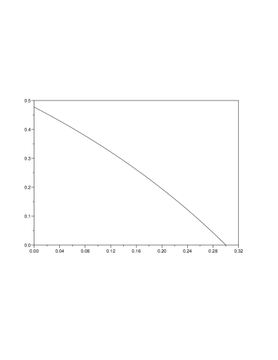
Figure 9: Plot of $P\left[{\rm m}_{x}>z,{\cal X}(\tau_{\mu}(x))=b\right]$ as a function of $z\in(0,x),$ for $b=1,\ \mu=1,\ r=1,\ x_{R}=1/4$ and $x=0.3\ .$ It decreases from the value $\pi_{b}(x)=\pi_{b}(0.3)=0.52286,$ attained at $z=0,$ to the value zero attained at $z=x=0.3\ .$

3 The inverse first-exit time (IFET) problem for BM with resetting

In this section, we study the IFET problem for (undrifted) BM with resetting, ${\cal X}(t),$ in a bounded interval $(0,b).$ Therefore, the underlying diffusion is $X(t)=\eta+W_{t},$ where the initial position $\eta={\cal X}(0)$ is supposed to be randomly distributed in $(0,b)$ and independent of ${\cal X}(t),$ whereas the reset rate $r>0$ and the reset position $x_{R}\in(0,b)$ are fixed. Actually, we omit to treat the case of drifted BM with resetting $(\mu,\ r\neq 0),$ because of heavier calculations.

We recall the terms of the IFET problem, mentioned in the Introduction.

Let $\tau(x)=\tau_{0}(x)$ be the FET of $\mathcal{X}(t)$ from $(0,b),$ under the condition that $\eta=x\in(0,b),$ namely

$$\tau(x)=\inf\{t>0:\mathcal{X}(t)\notin(0,b)|\eta=x\},$$ (3.1)

and let $\tau$ the (unconditional) FET of $\mathcal{X}(t)$ i.e.

$$\tau=\inf\{t>0:\mathcal{X}(t)\notin(0,b)\}.$$ (3.2)

For a given distribution function $F(t)$ on the positive real axis, or equivalently for a given FPT density $f(t)=F^{\prime}(t),\ t>0,$ the IFET problem consists in finding the density $g$ of the random initial position $\eta\in(0,b),$ if it exists, such that $P[\tau\leq t]=F(t),\ t>0.$ The function $g$ is called a solution to the IFET problem for $\mathcal{X}(t);$ in fact, the uniqueness of the solution is not guaranteed (see Example 5). For BM without resetting $(r=0),$ the IFET problem was studied in [14].

If $g(x)$ is the density of the random initial position $\eta,$ by using the explicit form (2.32) of the LT $M_{0}(x,\lambda)$ of $\tau(x),$ we obtain the LT of the FET $\tau:$

$$E\left[e^{-\lambda\tau}\right]=\int_{0}^{b}g(x)M_{0}(x,\lambda)dx$$

$$=\int_{0}^{b}g(x)\left\{1-\frac{\lambda\left[\sinh(\alpha_{\lambda}b)-\sinh(\alpha_{\lambda}x)-\sinh(\alpha_{\lambda}(b-x))\right]}{{\cal A}_{\lambda}}\right\}dx$$

$$=1-\frac{\lambda}{{\cal A}_{\lambda}}\int_{0}^{b}g(x)\left[\sinh(\alpha_{\lambda}b)-\sinh(\alpha_{\lambda}x)-\sinh(\alpha_{\lambda}(b-x))\right]dx,$$ (3.3)

or also

$$E\left[e^{-\lambda\tau}\right]=1-\frac{1}{{\cal A}_{\lambda}}\Big{\{}\lambda\sinh(\alpha_{\lambda}b)-\lambda E\left[\sinh(\alpha_{\lambda}\eta)+\sinh(\alpha_{\lambda}(b-\eta))\right]\Big{\}},$$ (3.4)

where

$${\cal A}_{\lambda}=\lambda\sinh(\alpha_{\lambda}b)+r\sinh(\alpha_{\lambda}x_{R})+r\sinh(\alpha_{\lambda}(b-x_{R})),$$

and

$$\alpha_{\lambda}=\sqrt{2(\lambda+r)}$$

(for simplicity, we omit to explicit the dependence of ${\cal A}_{\lambda}$ on $b,r,x_{R}$ and of $\alpha_{\lambda}$ on $r).$

Let us denote by $\widehat{g}(\theta)=\int_{0}^{b}e^{-\theta x}g(x)dx$ the (possibly bilateral) LT of $g(x).$ Then, from (3.3) we obtain the following:

Proposition 3.1

Let $\mathcal{X}(t)$ be (undrifted) BM with resetting, starting from the random initial position $\eta\in(0,b),$ which is supposed to be independent of $\mathcal{X}(t),$ and let $f(t),\ t>0,$ be a given FPT density. Then, if there exists a solution $g$ to the IFET problem for $\mathcal{X}(t),$ the following equality holds:

$$\widehat{f}(\lambda)=1-\frac{\lambda}{{\cal A}_{\lambda}}\left\{\sinh(\alpha_{\lambda}b)-\frac{1}{2}\left[\left(e^{\alpha_{\lambda}b}-1\right)\widehat{g}(\alpha_{\lambda})+\left(1-e^{-\alpha_{\lambda}b}\right)\widehat{g}(-\alpha_{\lambda})\right]\right\},\ \lambda>0,$$ (3.5)

$(\alpha_{\lambda}=\sqrt{2(\lambda+r)}).$

If one requires that $g$ is symmetric with respect to $x=b/2,$ that is, $g\left(\frac{b}{2}-u\right)=g\left(\frac{b}{2}+u\right),\ u\in(0,b/2),$ one finds $\widehat{g}(\theta)=e^{-b\theta}\widehat{g}(-\theta),\ \theta>0,$ and so (3.5) becomes:

$$\widehat{f}(\lambda)=1-\frac{\lambda}{{\cal A}_{\lambda}}\left[\sinh(\alpha_{\lambda}b)-(e^{\alpha_{\lambda}}-1)\widehat{g}(\alpha_{\lambda})\right],$$ (3.6)

or

$$\widehat{g}(\theta)=\frac{\Big{[}\left(\frac{\theta^{2}}{2}-r\right)\sinh(\theta b)+rs_{\lambda}\Big{]}\widehat{f}\left(\frac{\theta^{2}}{2}-r\right)-rs_{\lambda}}{(\frac{\theta^{2}}{2}-r)(e^{\theta b}-1)},$$ (3.7)

where

$$s_{\lambda}=\sinh(\alpha_{\lambda}x_{R})+\sinh(\alpha_{\lambda}(b-x_{R}))$$ (3.8)

(we omit the dependence of $s_{\lambda}$ on $b,r,x_{R}).$ $\Box$

Remark 3.2

For $r=0$ Eq. (3.7) coincides with Eq. (2.2) of [14].

If we set $\bar{T}=\max_{x\in(0,b)}E[\tau(x)],$ then from $E[\tau]=\int_{0}^{b}E[\tau(x)]g(x)dx,$ we get the compatibility condition

$$E[\tau]\leq\bar{T},$$ (3.9)

which is necessary so that a solution to the IFET problem exists.

Formula (3.5) provides a functional relation between the LT of $f$ and that of $g.$ Once $\widehat{g}$ has been found, such that it satisfies (3.5), it may be that $\widehat{g}$ is not the LT of the probability density function of a random variable. In this case, a solution to the IFET problem does not exist. This is the reason way Proposition 3.1 is formulated in a conditional form.

In the case when $g$ is symmetric with respect to $b/2,$ (3.7) allows to write $\widehat{g}(\theta)$ in terms of a function of $\widehat{f}(\theta)$ and other parameters. If $\widehat{f}$ is an analytic function, then $\widehat{g}$ is also analytic in the interval $(-\sqrt{2r},\sqrt{2r}),$ and so (3.7) uniquely identifies the density $g$, and hence the distribution of $\eta;$ therefore, if there is a solution to the IFET problem, then it is unique.

Thus, we conclude that, if $\widehat{f}$ is analytic, then the solution $g$ to the IFET problem is unique, under the constraint that it is sought in the class of densities that are symmetric with respect to $b/2.$

Now, we will prove the existence of a solution $g$ to the IFPT problem for a class of FPT densities $f.$ For the sake of simplicity, we limit ourselves to the case when $b=1,\ r=1,\ x_{R}=1/2$ and $g$ is symmetric with respect to $b/2=1/2.$

For any integer $k\geq 0,$ set $J_{k}(\theta)=\int_{0}^{1}e^{-\theta x}x^{k}dx;$ as easily seen, $J_{0}(\theta)=\frac{1-e^{-\theta}}{\theta}$ and the recursive relation $J_{k}(\theta)=\frac{k}{\theta}J_{k-1}(\theta)-\frac{e^{-\theta}}{\theta},\ k\geq 1$ allows to calculate $J_{k}(\theta),$ for every $k.$

The following Proposition gives a sufficient condition, in order that there exists a solution to the IFPT problem for BM with resetting.

Proposition 3.3

Let ${\cal X}(t)$ be (undrifted) BM with resetting, and let $b=1,\ r=1,\ x_{R}=1/2.$ Suppose that the LT of $f(t)$ has the form:

$$\widehat{f}(\lambda)=\sum_{k=1}^{N}p_{k}\widehat{f}_{k}(\lambda),\ \lambda>0,$$ (3.10)

where:

$$\widehat{f}_{k}(\lambda)=\frac{2\sinh(\alpha_{\lambda}/2)+\lambda(e^{\alpha_{\lambda}}-1)\widehat{g}_{k}(\alpha_{\lambda})}{\lambda\sinh(\alpha_{\lambda})+2\sinh(\alpha_{\lambda}/2)}\ \ (\alpha_{\lambda}=\sqrt{2(\lambda+r)}),$$ (3.11)

the numbers $p_{k}\geq 0$ are chosen in such a way that $\sum_{k=1}^{N}p_{k}=1,$

and

$$\widehat{g}_{k}(\lambda)=\frac{(2k+1)!}{(k!)^{2}}\sum_{i=0}^{k}(-1)^{i}\begin{pmatrix}k\\ i\end{pmatrix}J_{k+i}(\lambda),\ k\geq 0.$$ (3.12)

Then, there exists a solution $g$ to the IFPT problem for ${\cal X}(t)$, corresponding to the FPT density $f,$ and it results:

$$g(x)=\sum_{k=1}^{N}p_{k}g_{k}(x).$$ (3.13)

Note that the density $g_{k}$ corresponding to the LT (3.12) is the Beta density in the interval $(0,1)$ with parameters $\alpha=\beta=k+1,$ i.e.

$$g_{k}(x)=\frac{(2k+1)!}{(k!)^{2}}x^{k}(1-x)^{k},\ k\geq 0.$$ (3.14)

Proof. First, we observe that, if the density $g_{k},\ k=1,\dots N,$ is a solution to the IFPT problem corresponding to the FPT density $f_{k},$ then $g(x)=\sum_{k=1}^{N}p_{k}g_{k}(x),$ with $p_{k}\geq 0$ and $\sum_{k=1}^{N}p_{k}=1,$ solves the IFPT problem for the FPT density $f(t)=\sum_{k}p_{k}f_{k}(t).$ Thus, it is enough to verify that $g_{k}$ is a solution to the IFPT problem corresponding to $f_{k}.$ Since a simple calculation shows that the LT of $g_{k}$ is:

$$\widehat{g}_{k}(\lambda)=\frac{(2k+1)!}{(k!)^{2}}\sum_{i=0}^{k}(-1)^{i}\begin{pmatrix}k\\ i\end{pmatrix}J_{k+i}(\lambda),\ \lambda>0,$$ (3.15)

the verification follows by inserting $\widehat{g}_{k}$ and $\widehat{f}_{k}$ given by (3.11) into (3.6), with $b=1,\ r=1,\ x_{R}=1/2,$ because $g_{k}(x)$ is symmetric with respect to $x=1/2.$

$\Box$

In the next subsection, we show some explicit examples of solutions to the IFET problem for (undrifted) BM with resetting.

3.1 Some examples of solutions to the IFET problem

Example 1. Let ${\cal X}(t)$ be BM with resetting, and let $b=1,\ r=1,\ x_{R}=1/2;$ suppose that the LT of the FET $\tau$ is:

$$\widehat{f}(\lambda)=2\ \frac{\sqrt{2(\lambda+1)}\sinh\left(\frac{1}{2}\sqrt{2(\lambda+1)}\right)+\lambda\left(\cosh\left(\sqrt{2(\lambda+1)}\right)-1\right)}{\sqrt{2(\lambda+1)}\left[\lambda\sinh\left(\sqrt{2(\lambda+1)}\right)+2\sinh\left(\frac{1}{2}\sqrt{2(\lambda+1)}\right)\right]},\ \lambda>0.$$ (3.16)

We search for a solution to the IFET problem for $\mathcal{X}(t)$ in the set of probability densities $g$ in $(0,1)$ which are symmetric with respect to $1/2;$ we find that a solution $g$ is the uniform density in the interval $(0,1),$ i.e. $g(x)=\mathbb{I}_{(0,1)}(x).$ Since $\widehat{f}(\lambda)$ is analytic, from Remark 3.2 it follows that this is the only solution in the class of densities which are symmetric with respect to $1/2.$

To verify this, we can use (3.5) or (3.7): it is sufficient to substitute the various quantities and use that for the uniform density $g$ in $(0,1)$ one has $\widehat{g}(s)=(1-e^{-s})/s.$

The LT (3.16) cannot be inverted in closed form to obtain the corresponding FET density $f;$ however, we can get some qualitative characteristics of the distribution having density $f.$ In fact, from $\widehat{f}(\lambda)$ we easily obtain all the moments $m_{k}$ and the central ones $\mu_{k}$ of the corresponding distribution. By rounding the values to the third decimal digit, the mean of the distribution turns out to be $E[\tau]=0.175,$ while $E[\tau^{2}]=0.074,\ \ E[\tau^{3}]=0.047,\ \ E[\tau^{4}]=0.041\ .$ Thus, the first three central moments are $\mu_{2}=0.043,\ \mu_{3}=0.019,\ \mu_{4}=0.018,$ from which skewness $\gamma_{1}=\frac{\mu_{3}}{\mu_{2}^{3/2}}=2.139,$ and excess kurtosis coefficient $\gamma_{2}=\frac{\mu_{4}}{\mu_{2}^{2}}-3=6.632$ follow. Since skewness $\gamma_{1}$ is positive, the tail of the distribution is on the right side; moreover, the density $f(t)$ tends to zero, as $t\rightarrow+\infty,$ more slowly than the normal density does, because excess kurtosis $\gamma_{2}$ is positive.

A qualitative graph of the density $f(t),$ as a function of $t\geq 0,$ is shown in the Fig. 10.

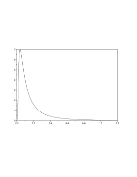
Figure 10: Qualitative graph of the FET density $f(t)$ corresponding to (3.16)

Example 2. Let ${\cal X}(t)$ be BM with resetting, and let $b=1,\ r=1,\ x_{R}=1/2,$ and suppose that the LT of the FET $\tau$ is:

$$\widehat{f}(\lambda)=\frac{2\sinh\left(\frac{1}{2}\sqrt{2(\lambda+1)}\right)+\lambda(e^{\sqrt{2(\lambda+1)}}-1)\widehat{g}_{1}(\sqrt{2(\lambda+1)})}{\lambda\sinh\left(\sqrt{2(\lambda+1)}\right)+2\sinh\left(\frac{1}{2}\sqrt{2(\lambda+1)}\right)},\ \lambda>0.$$ (3.17)

Then, a solution $g$ to the IFET problem for ${\cal X}(t)$ is the Beta density $g_{1}(x)=6x(1-x)\mathbb{I}_{(0,1)}(x).$ This is a special case of Proposition 3.3 for $N=k=1.$

Example 3. Let ${\cal X}(t)$ be BM with resetting, and let $b=1,\ r=1,\ x_{R}=1/2,$ and $\alpha,\beta>0;$ suppose that the LT of the FET $\tau$ is:

$$\widehat{f}(\lambda)=1-\left[\frac{\lambda}{\lambda\sinh(\alpha_{\lambda})+2\sinh(\alpha_{\lambda}/2)}\right]\times$$

$$\times\left\{\sum_{k=0}^{\infty}\frac{\alpha_{\lambda}^{2k+1}}{(2k+1)!}(\cosh(\alpha_{\lambda})-1)\frac{B(\alpha+k,\beta)}{B(\alpha,\beta)}-\sum_{k=1}^{\infty}\frac{\alpha_{\lambda}^{k}}{(2k)!}\sinh(\alpha_{\lambda})\frac{B(\alpha+k,\beta)}{B(\alpha,\beta)}\right\},$$ (3.18)

where $\alpha_{\lambda}=\sqrt{2(\lambda+r)}$ and

$$B(\alpha,\beta)=\frac{\Gamma(\alpha)\Gamma(\beta)}{\Gamma(\alpha+\beta)}.$$

Then, a solution $g$ to the IFET problem for ${\cal X}(t)$ is the Beta density in $(0,1)$ with parameters $\alpha$ and $\beta,$ namely $g(x)=\frac{\Gamma(\alpha+\beta)}{\Gamma(\alpha)\Gamma(\beta)}x^{\alpha-1}(1-x)^{\beta-1}\mathbb{I}_{(0,1)}(x).$ Example 1 and Example 2 are special cases, when $\alpha=\beta=1,$ and $\alpha=\beta=2,$ respectively.

To verify this by means of Proposition 3.1 it is sufficient to substitute the various quantities into (3.4) or (3.5); it is convenient to use that, if $\eta$ has Beta density in $(0,1),$ one has (see e.g. [23]):

$$E\left[e^{s\eta}\right]=\sum_{k=0}^{\infty}\frac{s^{k}}{k!}\frac{B(\alpha+k,\beta)}{B(\alpha,\beta)}.$$ (3.19)

Thus:

$$E\left[\sinh(s\eta)\right]=\sum_{k=0}^{\infty}\frac{s^{2k+1}}{(2k+1)!}\frac{B(\alpha+k,\beta)}{B(\alpha,\beta)},$$ (3.20)

and

$$E\left[\sinh(s(b-\eta))\right]=\sum_{k=0}^{\infty}\frac{s^{2k}}{(2k)!}\sinh(sb)\frac{B(\alpha+k,\beta)}{B(\alpha,\beta)}-\sum_{k=0}^{\infty}\frac{s^{2k+1}}{(2k+1)!}\cosh(sb)\frac{B(\alpha+k,\beta)}{B(\alpha,\beta)}.$$ (3.21)

Example 4. Let ${\cal X}(t)$ be BM with resetting, and let $b=1,\ x_{R}=1/2,$ and $\gamma$ a fixed positive number; suppose that the LT of the FET $\tau$ is, for $\lambda\neq\gamma^{2}/2-r:$

$$\widehat{f}(\lambda)=\frac{1}{\lambda\sinh(\sqrt{2(\lambda+r)})+r\left[\sinh(x_{R}\sqrt{2(\lambda+r)})+\sinh((1-x_{R})\sqrt{2(\lambda+r)})\right]}\times$$

$$\Biggl{\{}r\left[\sinh(x_{R}\sqrt{2(\lambda+r)})+\sinh((1-x_{R})\sqrt{2(\lambda+r)})\right]+$$ (3.22)

$$+\frac{\lambda\gamma}{2(e^{\gamma}-1)}\left[\frac{\left(e^{\sqrt{2(\lambda+r)}}-1\right)\left(e^{\gamma}-e^{-\sqrt{2(\lambda+r)}}\right)}{\gamma+\sqrt{2(\lambda+r)}}+\frac{\left(1-e^{-\sqrt{2(\lambda+r)}}\right)\left(e^{\gamma}-e^{\sqrt{2(\lambda+r)}}\right)}{\gamma-\sqrt{2(\lambda+r)}}\right]\Biggr{\}}.$$

Then, a solution $g$ to the IFET problem for ${\cal X}(t)$ is the exponential density with parameter $\gamma>0,$ truncated to the interval $(0,1),$ i.e. $g(x)=\frac{\gamma e^{-\gamma x}}{1-e^{-\gamma}}\mathbb{I}_{(0,1)}(x).$ To verify this by means of Proposition 3.1 it is sufficient to substitute the various quantities into (3.5), and to use that for this density $g$ one has $\widehat{g}(s)=\frac{\gamma(e^{\gamma}-e^{-s})}{(e^{\gamma}-1)(\gamma+s)}.$

Example 5. Let ${\cal X}(t)$ be BM with resetting, and let $b=1,\ r=1,\ x_{R}=1/2;$ suppose that the LT of the FET $\tau$ is given again by (3.16) of Example 1. Now, we seek for a solution $g$ to the IFET problem, without the constraint on the symmetry of $g$ with respect to $1/2;$ therefore, we must use (3.5). Then, we obtain that a solution to the IFET problem for ${\cal X}(t)$ is the density $g(x)=2x\mathbb{I}_{(0,1)}(x).$ This is easily verified by substituting the various quantities into (3.5), and using that for this density $g$ one has $\widehat{g}(s)=\frac{2}{s^{2}}(1-e^{s}(1-s)).$ Thus, for the LT $\widehat{f}$ given by (3.16), we have found two different solutions to the IFET problem: this last solution $g$ and that of Example 1.

This example shows that there is not uniqueness of the solution $g$ to the IFET problem, unless one does not introduce constraints on the class of densities $g.$

In the next example the solution to the IFET problem is a discrete density.

Example 6. Let ${\cal X}(t)$ be BM with resetting, and let $b=2,\ r=1,\ x_{R}=1/2;$ we suppose that the random initial position $\eta$ takes integer values in the set $\{0,\ 1,\ 2\},$ and that the LT of the FET $\tau$ is:

$$\widehat{f}(\lambda)=2\ \frac{\sinh\left(\frac{1}{2}\sqrt{2(\lambda+1)}\right)+\frac{\lambda}{3}\left[\sinh\left(\sqrt{2(\lambda+1)}\right)+\sinh\left(2\sqrt{2(\lambda+1)}\right)\right]}{\lambda\sinh\left(2\sqrt{2(\lambda+1)}\right)+2\sinh\left(\frac{1}{2}\sqrt{2(\lambda+1)}\right)}.$$ (3.23)

This LT cannot be inverted in closed form to obtain the corresponding FET density $f;$ however, the mean of the distribution turns out to be $E[\tau]=0.991,$ and $E[\tau^{2}]=8.148\ .$ We seek for a solution $g$ to the IFET problem, with the constraint that $g$ is symmetric with respect to $x=1;$ therefore, we can use (3.7). By substituting the various quantities into (3.7), we find that a solution $g$ to the IFET problem for ${\cal X}(t)$ with this constraint, is the discrete uniform density in the set $\{0,1,2\},$ namely $g(x)=\frac{1}{3},\ x\in\{0,\ 1,\ 2\},$ being $\widehat{g}(\lambda)=\frac{1}{3}(1+e^{-\lambda}+e^{-2\lambda}).$

4 Conclusions and Final Remarks

We studied the direct and inverse first-exit time (FET) problems for a one-dimensional diffusion process $\mathcal{X}(t)$ with resetting, obtained from an underlying temporally homogeneous diffusion $X(t)$ driven by the SDE $dX(t)=\mu(X(t))dt+\sigma(X(t))d{W_{t}},$ where $W_{t}$ is a standard Brownian motion, and the drift $\mu(\cdot)$ and diffusion coefficient $\sigma(\cdot)$ are regular enough functions, such that there exists a unique strong solution of the SDE. The process $\mathcal{X}(t)$ starts from $\mathcal{X}(0)=\eta\in(0,b)$ and it is subject to reset to the position $x_{R}$ according to a homogeneous Poisson process with rate $r>0.$

Thus, for any $C^{2}$ function $u(x),$ the infinitesimal generator $\mathcal{L}$ of ${\cal X}(t)$ is given by ${\cal L}u(x)=\frac{1}{2}\sigma^{2}(x)u^{\prime\prime}(x)+\mu(x)u^{\prime}(x)+r(u(x_{R})-u(x))=Lu(x)+r(u(x_{R})-u(x)),$ where $Lu(x)=\frac{1}{2}\sigma^{2}(x)u^{\prime\prime}(x)+\mu(x)u^{\prime}(x)$ represents the “diffusion part”, i.e. that concerning the diffusion $X(t).$

As regards the direct FET problem, for fixed $\eta=x\in(0,b)$ we investigated the statistical properties of the FET $\tau(x)$ of $\mathcal{X}(t)$ from the interval $(0,b),$ where $\tau(x)=\min\{t>0:\mathcal{X}(t)\notin(0,b)|\mathcal{X}(0)=x\};$ moreover, we studied the probability distribution of the first exit area FEA $A(x),$ namely the area swept out by ${\cal X}(t)$ till the time $\tau(x),$ and the probability distributions of the maximum and minimum displacement of ${\cal X}(t)$ for $t\in(0,\tau(x)).$

In particular, we stated ODEs with boundary conditions for the exit probability of $\mathcal{X}(t)$ from the left and right ends of the interval $(0,b),$ for the Laplace transforms of $\tau(x)$ and $A(x),$ for the single and joint moments of $\tau(x)$ and $A(x),$ and for the probability distributions of the maximum and minimum displacement of ${\cal X}(t)$ till the FET, all in terms of the infinitesimal generator ${\cal L}$ of $\mathcal{X}(t).$

In the case of drifted Brownian motion with resetting, namely when the diffusion and drift coefficients are $\sigma(x)=1$ and $\mu(x)=\mu,$ the generator turns out to be $\mathcal{L}u(x)=\frac{1}{2}u^{\prime\prime}(x)+\mu u^{\prime}(x)+r(u(x_{R})-u(x)),$ and the ODEs were explicitly solved in terms of elementary functions, except that concerning the Laplace transform of $A(x),$ that admits a solution only in terms of special functions.

As for the inverse first-exit time (IFET) problem for (undrifted) Brownian motion with resetting, we supposed that the starting position $\eta$ was randomly distributed in $(0,b),$ and we denoted by $\tau$ the FET of $\mathcal{X}(t)$ from the interval $(0,b);$ then, for a given distribution function $F(t)$ on the the time $t$ axis, the IFET problem consisted in finding the probability density $g$ of $\eta,$ if existing, such that the FET of $\mathcal{X}(t)$ from $(0,b)$ has distribution $F(t),$ namely $P[\tau\leq t]=F(t),\ t>0.$ The density $g$ was called a solution to the IFET problem for $\mathcal{X}(t);$ it turned out to be unique, under certain conditions. We reported several explicit examples of solutions to the IFET problem, for Brownian motion with resetting.

The case when $b=+\infty$ was studied in [3], while the two-barrier IFET problem for diffusions without resetting was studied in [14].

A different type of IFET problem for diffusions with resetting, consisting in finding the density $g$ of the starting position $\eta\in(0,b)$ corresponding to an assigned mean value of the FET $\tau,$ was studied in [2]; of course, in that case the solution $g$ was not unique.

We remark that the inverse problem here considered concerns randomization in the starting point $\eta$ of $\mathcal{X}(t).$ More generally, one could introduce randomization in the reset position $x_{R}$ (taking fixed $\eta),$ or both in the starting point $\eta$ and in the reset position $x_{R},$ and then study the corresponding IFET problems, where now a solution is the joint density of $(\eta,\ x_{R}),$ if it exist.

The feature of the present paper was to characterize several quantities concerning direct and inverse FET problems, as solutions of ODEs with boundary conditions, which can be explicitly solved in terms of elementary functions.

Although the calculations were developed for drifted Brownian motion with resetting, in principle they can be carried on for any one-dimensional diffusion with resetting, obtained from $X(t)$ driven by the SDE (1.1); it suffices to substitute the corresponding generator $Lu(x)=\frac{1}{2}\sigma^{2}(x)u^{\prime\prime}(x)+\mu(x)u^{\prime}(x)$ in all the ODEs.

For instance, one can study the case when the underlying diffusion $X(t)$ is conjugated to Brownian motion, namely there exists an increasing differentiable function $v(x)$ with $v(0)=0,$ such that $X(t)=v^{-1}\left(W_{t}+v(\eta)\right),$ for any $t\geq 0.$ (see [15]). Actually, if $\mathcal{X}(t)$ is obtained from a diffusion $X(t)$ which is conjugated to Brownian motion via the function $v$, the direct and inverse FET problems of $\mathcal{X}(t)$ are easily reduced to those of BM with resetting in the interval $(0,v(b)),$ starting from $v(\eta).$

Another diffusion with resetting that can be reduced to drifted BM with resetting is the process $\mathcal{X}(t),$ whose underlying diffusion is Geometric Brownian motion, that is driven by the SDE $dX(t)=\nu X(t)dt+\sigma X(t)dW_{t},\ \nu,\sigma>0.$ For other examples, see e.g. [2].

Moreover, the arguments of this article can also be applied, for example, to the Ornstein-Uhlenbeck process with stochastic resetting (see e.g. [19]), namely when the underlying diffusion $X(t)$ is driven by the SDE $dX(t)=-\nu X(t)+\sigma dB_{t},$ for positive constants $\nu$ and $\sigma.$ Of course, in this case the corresponding differential equations to obtain the various quantities are rather complicated, however they can be solved in principle.

Our study was motivated by the fact that, as in the case without resetting, direct and inverse problems for the FET of a diffusion process are worthy of attention, because they have notable applications in several applied fields, for instance in biological modeling concerning neuronal activity, queuing theory, and mathematical finance.

Acknowledgments: The author belongs to GNAMPA, the Italian National Research Group of INdAM; he also acknowledges the MUR Excellence Department Project MatMod@TOV awarded to the Department of Mathematics, University of Rome Tor Vergata, CUP E83C23000330006 .

References

- [1] Abramowitz, M., Stegun, I.A., 1965. Handbook of mathematical functions: With formulas, graphs, and mathematical tables. Dover, New York
- [2] Abundo, M., 2024. Inverse first-passage problems of a diffusion with resetting. Theor. Probability and Math. Statist . To appear.
- [3] Abundo, M., 2023. The first-passage area of a Wiener process with stochastic resetting. Methodol Comput Appl Probab 25:92 https://doi.org/10.1007/s11009-023-10069-4
- [4] Abundo, M., 2023. The first-passage area of Ornstein-Uhlenbeck process revisited. Stochastic Analysis and Applications 41(2): 358–376. https://doi.org/10.1080/07362994.2021.2018335.
- [5] Abundo, M., 2022. Some examples of solutions to an inverse problem for the first-passage place of a jump-diffusion process. Control Cybernetics vol. 51, No. 1, 31–42. DOI: 10.2478/candc-2022-0003
- [6] Abundo, M., 2020. An inverse problem for the first-passage place of some diffusion processes with random starting point. Stochastic Anal. Appl. vol. 38, No. 6, 1122–1133. https://doi.org/10.1080/07362994.2020.1768867
- [7] Abundo, M., 2019. An inverse first-passage problem revisited: the case of fractional Brownian motion, and time-changed Brownian motion. Stochastic Anal. Appl. vol. 37, No. 5, 708–716, https://doi.org/10.1080/07362994.2019.1608834
- [8] Abundo, M., 2018. The Randomized First-Hitting Problem of Continuously Time-Changed Brownian Motion. Mathematics 6(6), 91, 1–10. https://doi.org/10.3390/math6060091
- [9] Abundo, M. and Del Vescovo, D, 2017. On the joint distribution of first-passage time and first-passage area of drifted Brownian motion. Methodol Comput Appl Probab 19:985–996 DOI 10.1007/s11009-017-9546-7
- [10] Abundo, M., 2015. An overview on inverse first-passage-time problems for one-dimensional diffusion processes. Lecture Notes of Seminario Interdisciplinare di Matematica Vol. 12, 1 – 44. http://dimie.unibas.it/site/home/info/documento3012448.html
- [11] Abundo, M., 2014. One-dimensional reflected diffusions with two boundaries and an inverse first-hitting problem. Stochastic Anal. Appl. 32, 975-991. DOI: 10.1080/07362994.2014.959595
- [12] Abundo, M., 2013. On the first-passage area of a one-dimensional jump-diffusion process. Methodol Comput Appl Probab 15:85–103
- [13] Abundo, M., 2013. Solving an inverse first-passage-time problem for Wiener process subject to random jumps from a boundary. Stochastic Anal. Appl. 31: 4, 695–707.
- [14] Abundo, M., 2013. The double-barrier inverse first-passage problem for Wiener process with random starting point. Stat. and Probab. Letters 83, 168–176.
- [15] Abundo, M., 2012. An inverse first-passage problem for one-dimensional diffusion with random starting point. Stat. and Probab. Letters 82, 7–14. Erratum: Stat. and Probab. Letters, 82(3), 705.
- [16] Abundo, M., 2000. On first-passage-times for one-dimensional jump-diffusion processes. Prob. Math.Statis. 20(2), 399–423.
- [17] Borodin, A.N., Salminen, S., 1996. Handbook of Brownian motion-facts and formulae. Birkhauser Verlag Basel, Basel
- [18] Darling, D.A., Siegert, A.J.F., 1953. The first passage problem for a continuous Markov process. Ann Math Stat 24:624–639.
- [19] Dubey, A. and Pal, A. (2023) First-passage functionals for Ornstein Uhlenbeck process with stochastic resetting. J Phys A: Math Theor 56 (1–19):435002. https://doi.org/10.1088/1751-8121/acf748
- [20] Di Crescenzo, A., Giorno, V., and Nobile, A.G. 2003. On the M/M/1 Queue with Catastrophes and Its Continuous Approximation. Queueing Systems 43, 329–347.
- [21] Gihman, I.I., Skorohod, A.V., 1972. Stochastic differential equations. Springer, Berlin
- [22] Guo, W., Yan, H., and Chen, H. 2024. Extremal statistics for for first-passage trajectories of drifted Brownian motion under stochastic resetting. J. Stat. Mech. 023209, 1–19. https://doi.org/10.1088/1742-5468/ad2678.
- [23] Gupta, A.K. (Ed.), Nadarajah, S. (Ed.), 2004. Handbook of Beta Distribution and Its Applications. Boca Raton: CRC Press. https://doi.org/10.1201/9781482276596.
- [24] Huang, F., and Chen, H. 2024. Extremal value statistics of first-passage trajectories of resetting Brownian motion in an interval. J. Stat. Mech. 093212, 1–21. https://doi.org/10.1088/1742-5468/ad7852.
- [25] Jackson, K., Kreinin, A., and Zhang, W., 2009. Randomization in the first hitting problem. Stat. and Probab. Letters 79, 2422–2428.
- [26] Karlin, S., Taylor, H.M., 1981. A Second Course in Stochastic Processes Elsevier.
- [27] Klebaner, F.C., 2005. Introduction to Stochastic Calculus with Applications, 2nd ed. London, Imperial College Press.
- [28] Lanska, V. and Smiths C.E., 1989. The effect of a random initial value in neural first-passage-time models. Math. Biosci. 93, 191–215.
- [29] Lefebvre, M., 2019. Moments of First-Passage Places for Jump-Diffusion Processes. Sankhya A, 1–9. https://doi.org/10.1007/s13171-019-00181-4
- [30] Lefebvre, M., 2022. The inverse first-passage-place problem for Wiener processes. Stochastic Anal. Appl., vol. 40, (1), 96–102.
- [31] Majumdar, S.N., 2007. Brownian functionals in physics and computer science. In The Legacy Of Albert Einstein: A Collection of Essays in Celebration of the Year of Physics (pp. 93-129).
- [32] Nobile, A.G., Ricciardi, L.M., and Sacerdote, L., 1985. Exponential trends of Ornstein-Uhlenbeck first-passage-time densities. J. Appl. Prob. 22, 360–369.
- [33] Singh, P. and Pal, 2022. First-passage Brownian functionals with stochastic resetting. J. Phys. A: Math. Theor. 55 234001: 1–25. https://doi.org/10.1088/1751-8121/ac677c
- [34] Tuckwell, H.C., 1976. On the first-exit time problem for temporally homogeneous Markov processes. J. Appl. Probab. 13, 39–48.