Sequential Extremal Principle and Necessary Conditions for Minimizing Sequences

Abstract

The conventional definition of extremality of a finite collection of sets is extended by replacing a fixed point (extremal point) in the intersection of the sets by a collection of sequences of points in the individual sets with the distances between the corresponding points tending to zero. This allows one to consider collections of unbounded sets with empty intersection. Exploiting the ideas behind the conventional extremal principle, we derive an extended sequential version of the latter result in terms of Fréchet and Clarke normals. Sequential versions of the related concepts of stationarity, approximate stationarity and transversality of collections of sets are also studied. As an application, we establish sequential necessary conditions for minimizing (and more general firmly stationary, stationary and approximately stationary) sequences in a constrained optimization problem.

49J52; 49J53; 49K40; 90C30; 90C46

1 Introduction

We continue studying extremality and stationarity properties of collections of sets and the corresponding generalized separation statements in the sense of the extremal principle [1, 2, 3]. Such statements are widely used in variational analysis and naturally translate into necessary optimality conditions (multiplier rules) and various subdifferential and coderivative calculus results in nonconvex settings [1, 4, 2, 5, 3, 6, 7].

Throughout the paper we consider a collection of $n>1$ arbitrary nonempty subsets $\Omega_{1},\ldots,\Omega_{n}$ of a normed space $(X,\|\cdot\|)$ and write $\{\Omega_{1},\ldots,\Omega_{n}\}$ to denote the collection of these sets as a single object.

The conventional extremal principle gives necessary conditions for the extremality of a collection of sets.

Definition 1.1 (Extremality).

The collection $\{\Omega_{1},\ldots,\Omega_{n}\}$ is extremal at $\bar{x}\in\bigcap_{i=1}^{n}\Omega_{i}$ if there is a $\rho\in(0,+\infty]$ such that, for any $\varepsilon>0$, there exist $a_{1},\ldots,a_{n}\in\varepsilon\mathbb{B}_{X}$ such that

$$\bigcap_{i=1}^{n}(\Omega_{i}-a_{i})\cap B_{\rho}(\bar{x})=\emptyset.$$ (1)

Here, symbols $\mathbb{B}_{X}$ and $B_{\rho}(\bar{x})$ denote the open unit ball in $X$ and open ball with centre $\bar{x}$ and radius $\rho$, respectively. For brevity, we combine in the above definition the cases of local ($\rho<+\infty$) and global ($\rho=+\infty$) extremality. In the latter case, the point $\bar{x}$ plays no role apart from ensuring that $\bigcap_{i=1}^{n}\Omega_{i}\neq\emptyset$.

The extremal principle gives necessary conditions for extremality in terms of elements of the (topologically) dual space $X^{*}$, and assumes that $X$ is Asplund and the sets are closed.

Theorem 1.2 (Extremal principle).

Let $X$ be Asplund, and $\Omega_{1},\ldots,\Omega_{n}$ be closed. If $\{\Omega_{1},\ldots,\Omega_{n}\}$ is extremal at $\bar{x}\in\bigcap_{i=1}^{n}\Omega_{i}$, then, for any $\varepsilon>0$, there exist $x_{i}\in\Omega_{i}\cap B_{\varepsilon}(\bar{x})$ and $x_{i}^{*}\in N^{F}_{\Omega_{i}}(x_{i})$ $(i=1,\ldots,n)$ such that

$$\Big{\|}\sum_{i=1}^{n}x_{i}^{*}\Big{\|}<\varepsilon,\quad\sum_{i=1}^{n}\|x_{i}^{*}\|=1.$$ (2)

Theorem 1.2 employs Fréchet normal cones (see definition (9)). The dual conditions are formulated in a fuzzy form and can be interpreted as generalized separation; cf. [8]. The statement naturally yields the limiting version of the extremal principle in terms of limiting normal cones [1, 4, 2, 5, 3]. In finite dimensions, the limiting version comes for free, while in infinite dimensions, additional sequential normal compactness type assumptions are required to ensure that the equality in (2) is preserved when passing to limits (as $\varepsilon\downarrow 0$); cf. [3].

The conventional extremal principle was established in this form in [2] as an extension of the original result from [1], which had been formulated in Fréchet smooth spaces and referred to as the generalized Euler equation. The proof employs the Ekeland variational principle [9] and fuzzy Fréchet subdifferential sum rule due to Fabian [10]. It was also shown in [2] that the necessary conditions in Theorem 1.2 are equivalent to the Asplund property of the space (see also [3, Theorem 2.20]). Recall that a Banach space is Asplund if every continuous convex function on an open convex set is Fréchet differentiable on a dense subset, or equivalently, if the dual of each its separable subspace is separable. We refer the reader to [11, 3, 7] for discussions about and characterizations of Asplund spaces. All reflexive, particularly, all finite dimensional Banach spaces are Asplund.

Definition 1.1 and Theorem 1.2 can be reformulated in the setting of the product space $X^{n}$ for the “aggregate” set $\widehat{\Omega}:=\Omega_{1}\times\ldots\times\Omega_{n}$ employing the maximum norm on $X^{n}$ and the corresponding dual (sum) norm:

$$\left|\kern-1.07639pt\left|\kern-1.07639pt\left|(u_{1},\ldots,u_{n})\right|\kern-1.07639pt\right|\kern-1.07639pt\right|:=\max_{1\leq i\leq n}\|u_{i}\|\quad\mbox{for all}\quad u_{1},\ldots,u_{n}\in X,$$ (3)

$$\left|\kern-1.07639pt\left|\kern-1.07639pt\left|(u_{1}^{*},\ldots,u_{n}^{*})\right|\kern-1.07639pt\right|\kern-1.07639pt\right|:=\sum_{1=1}^{n}\|u_{i}^{*}\|\quad\mbox{for all}\quad u_{1}^{*},\ldots,u_{n}^{*}\in X^{*}.$$ (4)

It was observed in [12] that Theorem 1.2 and its numerous generalizations and extensions remain valid with an arbitrary product norm $\left|\kern-1.07639pt\left|\kern-1.07639pt\left|\,\cdot\,\right|\kern-1.07639pt\right|\kern-1.07639pt\right|$ (together with the corresponding dual norm) satisfying natural compatibility conditions with the original norm $\|\cdot\|$ on $X$. This more general setting, in particular, allows one to recapture the unified separation theorem of Zheng & Ng [13, 14] employing the $p$-weighted nonintersect index, and its slightly more advanced version in [15].

In this paper, following the scheme initiated in [12], we assume that $X^{n}$ is equipped with a norm $\left|\kern-1.07639pt\left|\kern-1.07639pt\left|\,\cdot\,\right|\kern-1.07639pt\right|\kern-1.07639pt\right|$ satisfying the following compatibility conditions:

$$\kappa_{1}\max_{1\leq i\leq n}\|u_{i}\|\leq\left|\kern-1.07639pt\left|\kern-1.07639pt\left|(u_{1},\ldots,u_{n})\right|\kern-1.07639pt\right|\kern-1.07639pt\right|\leq\kappa_{2}\max_{1\leq i\leq n}\|u_{i}\|\quad\text{for all}\;\;u_{1},\ldots,u_{n}\in X$$ (5)

with some $\kappa_{1}>0$ and $\kappa_{2}>0$. For a discussion of weaker compatibility conditions and some results without such conditions we refer the reader to [12]. Clearly, the norm (3) satisfies conditions (5). Under (5), if $X$ is Banach/Asplund, then so is $X^{n}$, and the (Fréchet or Clarke) normal cone to $\widehat{\Omega}$ equals the cartesian product of the corresponding cones to the individual sets; see [12].

The next definition contains abstract product norm extensions of the extremality property in Definition 1.1 and corresponding stationarity properties studied in [16, 17, 5, 18, 19, 20, 21, 22]. Given a $u\in X$, we write $(u,\ldots,u)_{n}$ to specify that $(u,\ldots,u)\in X^{n}$.

Definition 1.3 (Extremality, stationarity and approximate stationarity).

Let $\bar{x}\in\bigcap_{i=1}^{n}\Omega_{i}$. The collection $\{\Omega_{1},\ldots,\Omega_{n}\}$ is

1. extremal at $\bar{x}$ if there is a $\rho\in(0,+\infty]$ such that, for any $\varepsilon>0$, there exists a point $(a_{1},\ldots,a_{n})\in\varepsilon\mathbb{B}_{X^{n}}$ such that condition (1) is satisfied;

2. stationary at $\bar{x}$ if, for any $\varepsilon>0$, there exist a $\rho\in(0,\varepsilon)$ and a point $(a_{1},\ldots,a_{n})\in\varepsilon\rho\mathbb{B}_{X^{n}}$ such that condition (1) is satisfied;

3. approximately stationary at $\bar{x}$ if, for any $\varepsilon>0$, there exist a $\rho\in(0,\varepsilon)$, and points $(x_{1},\ldots,x_{n})\in\widehat{\Omega}\cap B_{\varepsilon}((\bar{x},\ldots,\bar{x})_{n})$ and $(a_{1},\ldots,a_{n})\in\varepsilon\rho\mathbb{B}_{X^{n}}$ such that

   $$\bigcap_{i=1}^{n}(\Omega_{i}-x_{i}-a_{i})\cap(\rho\mathbb{B})=\emptyset.$$ (6)

The relationships between the properties in Definition 1.3 are straightforward: (i) $\Rightarrow\$(ii) $\Rightarrow\$(iii). The approximate stationarity, the weakest of the three properties, is still sufficient for the generalized separation in Theorem 1.2 in Asplund spaces. The two properties are actually equivalent. The next statement from [12] generalizes the extended extremal principle [5, Theorem 3.7].

Theorem 1.4 (Extended extremal principle).

Let $X$ be Asplund, $\Omega_{1},\ldots,\Omega_{n}$ be closed, and $\bar{x}\in\bigcap_{i=1}^{n}\Omega_{i}$. The collection $\{\Omega_{1},\ldots,\Omega_{n}\}$ is approximately stationary at $\bar{x}$ if and only if, for any $\varepsilon>0$, there exist $x_{i}\in\Omega_{i}\cap B_{\varepsilon}(\bar{x})$ and $x_{i}^{*}\in N^{F}_{\Omega_{i}}(x_{i})$ $(i=1,\ldots,n)$ such that

$$\Big{\|}\sum_{i=1}^{n}x_{i}^{*}\Big{\|}<\varepsilon,\quad\left|\kern-1.07639pt\left|\kern-1.07639pt\left|\hat{x}^{*}\right|\kern-1.07639pt\right|\kern-1.07639pt\right|=1,$$ (7)

where $\hat{x}^{*}:=(x_{1}^{*},\ldots,x_{n}^{*})$.

The conventional concept of extremality of a collection of sets in Definition 1.1 as well as its generalizations and extensions in Definition 1.3 and corresponding characterizations in Theorems 1.2 and 1.4 are attached to a fixed point in the intersection of the sets (often referred to as extremal point). Despite its recognized versatility and numerous applications, this model does not cover an important class of problems involving unbounded sets, for which some analogues of the extremality, stationarity and generalized separation properties may still hold “approximately” with a common point of the sets replaced by unbounded sequences. This can be illustrated by the following example of a pair of unbounded sets in $\mathbb{R}^{2}$.

Example 1.5.

Let $X:=\mathbb{R}^{2}$. Consider closed convex sets $\Omega_{1}:=\{(x,y)\mid x>0,\;xy\geq 1\}$ and $\Omega_{2}:=\{(x,y)\mid y\leq 0\}$; see Figure 1. We have $d(\Omega_{1},\Omega_{2})=0$ while $\Omega_{1}\cap\Omega_{2}=\emptyset$. At the same time, for any $\varepsilon>0$, $t>\varepsilon^{-1}$ and $\xi\in(\frac{1}{t},\varepsilon)$, taking $x_{1}:=(t,\frac{1}{t})\in\Omega_{1}$, $x_{2}:=(t,0)\in\Omega_{2}$, $a_{1}:=(0,-\xi)$ and $a_{2}:=(0,0)$, one has $(\Omega_{1}-x_{1}-a_{1})\cap(\Omega_{2}-x_{2}-a_{2})=\emptyset$. This can be interpreted as an approximate version of the conditions in Definition 1.1 with $\rho=+\infty$ and the pair of points $x_{1}\in\Omega_{1}$ and $x_{2}\in\Omega_{2}$ (depending on $t$) replacing the nonexistent common point $\bar{x}$. Note that $\|x_{1}\|\to+\infty$, $\|x_{2}\|\to+\infty$ and $\|x_{1}-x_{2}\|\to 0$ as $t\to+\infty$.

Moreover, assuming for simplicity that $\mathbb{R}^{2}$ is equipped with the maximum norm, for any $\varepsilon>0$, taking a $t>\max\{\frac{1}{\sqrt{2\varepsilon}},1\}$, and points $x_{1}:=(t,\frac{1}{t})\in\Omega_{1}$ and $x_{2}:=(t,0)\in\Omega_{2}$ as above, we have $x_{1}^{*}:=(-\frac{1}{2t^{2}},-\frac{1}{2})\in N_{\Omega_{1}}(x_{1})$, $x_{2}^{*}:=(0,\frac{1}{2})\in N_{\Omega_{2}}(x_{2})$, $\|x_{1}^{*}\|=\|x_{2}^{*}\|=\frac{1}{2}$ and $\|x_{1}^{*}+x_{2}^{*}\|=\frac{1}{2t^{2}}<\varepsilon$, i.e., the conclusions of Theorem 1.2 hold approximately, with the pair of points $x_{1}\in\Omega_{1}$ and $x_{2}\in\Omega_{2}$ replacing the nonexistent common point $\bar{x}$.

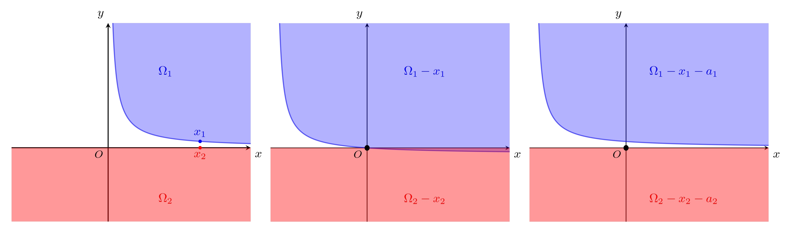
Figure 1: Example 1.5

This paper, motivated by the recent research targeting optimality conditions and subdifferential/coderivative calculus “at infinity” in [23, 24], extends the model in Definition 1.3 to cover the case of a collection of unbounded sets satisfying

$$d(\Omega_{1},\ldots,\Omega_{n}):=\inf_{x_{1}\in\Omega_{1},\ldots,x_{n}\in\Omega_{n}}{\rm diam}\,\{x_{1},\ldots,x_{n}\}=0,$$ (8)

where ${\rm diam}\,\{x_{1},\ldots,x_{n}\}:=\max_{1\leq i,j\leq n}\|x_{i}-x_{j}\|$ is the diameter of the set $\{x_{1},\ldots,x_{n}\}$. The common point of the sets $\Omega_{1},\ldots,\Omega_{n}$ (which may not exist) is replaced in the corresponding definitions and characterizations by appropriate sequences.

The new extended model is discussed in Section 2, where sequential versions of the extremality, stationarity and approximate stationarity concepts for a finite collection of sets in a normed vector space are introduced. The corresponding generalized separation conditions including the sequential extremal principle are established in Section 3. To illustrate the model, we consider in Section 4 a constrained optimization problem and discuss sequential minimality and stationarity properties. Employing the sequential extremal principle, we deduce in Section 5 sequential optimality and stationarity conditions for the considered constrained optimization problem. The final Section 6 summarises the contributions of the paper and lists potential directions of future research.

Preliminaries

Our basic notation is standard, see, e.g., [3, 7]. The topological dual of a normed space $X$ is denoted by $X^{*}$, while $\langle\cdot,\cdot\rangle$ denotes the bilinear form defining the pairing between the two spaces. Symbols $\mathbb{B}$ (possibly with a subscript indicating the space) and $B_{\rho}(\bar{x})$ denote the open unit ball and open ball with centre $\bar{x}$ and radius $\rho$, respectively, while $\overline{\mathbb{B}}$ denotes the closed unit ball. If $(x,y)\in X\times Y$, we write $B_{\varepsilon}(x,y)$ instead of $B_{\varepsilon}((x,y))$. Symbols $\mathbb{R}$, $\mathbb{R}_{+}$ and $\mathbb{N}$ stand for the sets of all, respectively, real, nonnegative real and positive integer numbers. The notation $\{x^{k}\}\subset\Omega$ denotes a sequence of points $x^{k}\in\Omega$ $(k\in\mathbb{N})$.

We consider the normed spaces $(X,\|\cdot\|)$ and $(X^{n},\left|\kern-1.07639pt\left|\kern-1.07639pt\left|\,\cdot\,\right|\kern-1.07639pt\right|\kern-1.07639pt\right|)$ with the norm compatibility condition (5), and the “aggregate” set $\widehat{\Omega}:=\Omega_{1}\times\ldots\times\Omega_{n}$. As the meaning will always be clear from the context, we keep the same notations $\|\cdot\|$ and $\left|\kern-1.07639pt\left|\kern-1.07639pt\left|\,\cdot\,\right|\kern-1.07639pt\right|\kern-1.07639pt\right|$ for the corresponding norms on $X^{*}$ and $(X^{*})^{n}$, and use $d(\cdot,\cdot)$ to denote distances (including point-to-set and set-to-set distances) in all spaces determined by the corresponding norms.

Normal cones and subdifferentials.

We first recall the definitions of normal cones and subdifferentials in the sense of Fréchet and Clarke; see, e.g., [25, 5, 3]. Given a subset $\Omega$ of a normed space $X$ and a point $\bar{x}\in\Omega$, the sets

$$N_{\Omega}^{F}(\bar{x}):=\Big{\{}x^{\ast}\in X^{\ast}\mid\limsup_{\Omega\ni x{\rightarrow}\bar{x},\;x\neq\bar{x}}\frac{\langle x^{\ast},x-\bar{x}\rangle}{\|x-\bar{x}\|}\leq 0\Big{\}},$$ (9)

$$N_{\Omega}^{C}(\bar{x}):=\left\{x^{\ast}\in X^{\ast}\mid\left\langle x^{\ast},z\right\rangle\leq 0\;\;\text{for all}\;\;z\in T_{\Omega}^{C}(\bar{x})\right\}$$ (10)

are the, respectively, Fréchet and Clarke normal cones to $\Omega$ at $\bar{x}$. Symbol $T_{\Omega}^{C}(\bar{x})$ in (10) stands for the Clarke tangent cone to $\Omega$ at $\bar{x}$:

$$T_{\Omega}^{C}(\bar{x}):=\big{\{}z\in X\mid\forall x_{k}{\rightarrow}\bar{x},\;x_{k}\in\Omega,\;\forall t_{k}\downarrow 0,\;\exists z_{k}\to z\;\;\text{with}\;\;x_{k}+t_{k}z_{k}\in\Omega\;\;\text{for all}\;\;k\in\mathbb{N}\big{\}}.$$

The sets (9) and (10) are nonempty closed convex cones satisfying $N_{\Omega}^{F}(\bar{x})\subset N_{\Omega}^{C}(\bar{x})$. If $\Omega$ is a convex set, they reduce to the normal cone $N_{\Omega}(\bar{x})$ in the sense of convex analysis.

For an extended-real-valued function $f:X\to\mathbb{R}_{\infty}:=\mathbb{R}\cup\{+\infty\}$ on a normed space $X$, its domain and epigraph are defined, respectively, by ${\rm dom}\,f:=\{x\in X\mid f(x)<+\infty\}$ and ${\rm epi}\,f:=\{(x,\alpha)\in X\times\mathbb{R}\mid f(x)\leq\alpha\}$. The Fréchet and Clarke subdifferentials of $f$ at $\bar{x}\in{\rm dom}\,f$ are defined, respectively, by

$$\partial^{F}f(\bar{x}):=\left\{x^{*}\in X^{*}\mid(x^{*},-1)\in N^{F}_{{\rm epi}\,f}(\bar{x},f(\bar{x}))\right\},$$ (11)

$$\partial^{C}{f}(\bar{x}):=\left\{x^{\ast}\in X^{\ast}\mid(x^{*},-1)\in N_{{\rm epi}\,f}^{C}(\bar{x},f(\bar{x}))\right\}.$$ (12)

The sets (11) and (12) are closed and convex, and satisfy $\partial^{F}{f}(\bar{x})\subset\partial^{C}{f}(\bar{x})$. If $f$ is convex, they reduce to the subdifferential $\partial f(\bar{x})$ in the sense of convex analysis.

Generalized separation.

The next generalized separation statement is the key tool in the proof of our main result. It is a simplified local version of a more general separation statement from [12].

Theorem 1.6 (Generalized separation).

Let $X$ be Banach, $\Omega_{1},\ldots,\Omega_{n}$ be closed, $\widehat{\omega}\in\widehat{\Omega}$, $\hat{x}^{\circ}:=(x^{\circ}_{1},\ldots,x^{\circ}_{n})\in X^{n}$, $\varepsilon>0$, $\delta>0$ and $\rho>0$. Suppose that ${\bigcap}_{i=1}^{n}(\Omega_{i}-x^{\circ}_{i})\cap(\rho\overline{\mathbb{B}})=\emptyset$, and $\left|\kern-1.07639pt\left|\kern-1.07639pt\left|\widehat{\omega}-\hat{x}^{\circ}\right|\kern-1.07639pt\right|\kern-1.07639pt\right|<\varepsilon$. The following assertions hold true:

1. there exist points $\hat{x}:=(x_{1},\ldots,x_{n})\in\widehat{\Omega}\cap B_{\delta}(\widehat{\omega})$, $x_{0}\in\rho\mathbb{B}$ and $\hat{x}^{*}:=(x_{1}^{*},\ldots,x_{n}^{*})\in(X^{*})^{n}$ such that $\left|\kern-1.07639pt\left|\kern-1.07639pt\left|\hat{x}^{*}\right|\kern-1.07639pt\right|\kern-1.07639pt\right|=1$, and

   $${\delta}d\left(\hat{x}^{*},N^{C}_{\widehat{\Omega}}(\hat{x})\right)+\rho\Big{\|}\sum_{i=1}^{n}x_{i}^{*}\Big{\|}<{\varepsilon},$$

   $$\left\langle\hat{x}^{*},(x_{0},\dots,x_{0})_{n}+\hat{x}^{\circ}-\hat{x}\right\rangle=\left|\kern-1.07639pt\left|\kern-1.07639pt\left|(x_{0},\dots,x_{0})_{n}+\hat{x}^{\circ}-\hat{x}\right|\kern-1.07639pt\right|\kern-1.07639pt\right|;$$

2. if $X$ is Asplund, then, for any $\tau\in(0,1)$, there exist points $\hat{x}:=(x_{1},\ldots,x_{n})\in\widehat{\Omega}\cap B_{\delta}(\widehat{\omega})$, $x_{0}\in\rho\mathbb{B}$ and $\hat{x}^{*}:=(x_{1}^{*},\ldots,x_{n}^{*})\in(X^{*})^{n}$ such that $\left|\kern-1.07639pt\left|\kern-1.07639pt\left|\hat{x}^{*}\right|\kern-1.07639pt\right|\kern-1.07639pt\right|=1$, and

   $${\delta}d\left(\hat{x}^{*},N^{F}_{\widehat{\Omega}}(\hat{x})\right)+\rho\Big{\|}\sum_{i=1}^{n}x_{i}^{*}\Big{\|}<{\varepsilon},$$

   $$\left\langle\hat{x}^{*},(x_{0},\dots,x_{0})_{n}+\hat{x}^{\circ}-\hat{x}\right\rangle>\tau\left|\kern-1.07639pt\left|\kern-1.07639pt\left|(x_{0},\dots,x_{0})_{n}+\hat{x}^{\circ}-\hat{x}\right|\kern-1.07639pt\right|\kern-1.07639pt\right|.$$

Similar to the conventional extremal principle, the latter statement is a consequence of the Ekeland variational principle and corresponding subdifferential sum rules. With the appropriate product space norms, it covers the unified separation theorems by Zheng & Ng [13, 14] and their slightly more advanced versions in [15]. Theorem 1.6 combines two assertions: the traditional Asplund space one covering Theorems 1.2 and 1.4 in part (ii) and the general Banach space assertion in terms of Clarke normal cones in part (i).

Remark 1.7.

Theorem 1.6 remains true if the assumption $\left|\kern-1.07639pt\left|\kern-1.07639pt\left|\widehat{\omega}-\hat{x}^{\circ}\right|\kern-1.07639pt\right|\kern-1.07639pt\right|<\varepsilon$ is replaced by the next weaker one (see [12]): $\left|\kern-1.07639pt\left|\kern-1.07639pt\left|\widehat{\omega}-\hat{x}^{\circ}\right|\kern-1.07639pt\right|\kern-1.07639pt\right|<\inf_{\begin{subarray}{c}\hat{u}\in\widehat{\Omega},\;u\in\rho\mathbb{B}\end{subarray}}\left|\kern-1.07639pt\left|\kern-1.07639pt\left|\hat{u}-\hat{x}^{\circ}-(u,\ldots,u)_{n}\right|\kern-1.07639pt\right|\kern-1.07639pt\right|+\varepsilon$.

2 Sequential extremality, stationarity and approximate stationarity

In this section, we discuss sequential versions of the extremality, stationarity and approximate stationarity concepts for a finite collection of sets in a normed vector space.

In what follows, the sets $\Omega_{1},\ldots,\Omega_{n}$ are not supposed to have a common point. Instead, we assume that $d(\Omega_{1},\ldots,\Omega_{n})=0$ (see (8)), i.e., there exist sequences $\{x_{i}^{k}\}\subset\Omega_{i}$ $(i=1,\ldots,n)$ such that ${\rm diam}\,\{x_{1}^{k},\ldots,x_{n}^{k}\}\to 0$ as $k\to+\infty$. The sequences may be unbounded.

The next definition is a modification of Definition 1.3 employing sequences of the type described above.

Definition 2.1 (Sequential extremality, stationarity and approximate stationarity).

The collection $\{\Omega_{1},\ldots,\Omega_{n}\}$ is

1. extremal at sequences $\{x_{i}^{k}\}\subset\Omega_{i}$ $(i=1,\ldots,n)$ if ${\rm diam}\,\{x_{1}^{k},\ldots,x_{n}^{k}\}\to 0$ as $k\to+\infty$, and there is a $\rho\in(0,+\infty]$ such that, for any $\varepsilon>0$, there exist an integer $k>\varepsilon^{-1}$ and a point $(a_{1},\ldots,a_{n})\in\varepsilon\mathbb{B}_{X^{n}}$ such that

   $$\bigcap_{i=1}^{n}(\Omega_{i}-x_{i}^{k}-a_{i})\cap(\rho\mathbb{B})=\emptyset.$$ (13)

2. stationary at sequences $\{x_{i}^{k}\}\subset\Omega_{i}$ $(i=1,\ldots,n)$ if ${\rm diam}\,\{x_{1}^{k},\ldots,x_{n}^{k}\}\to 0$ as $k\to+\infty$, and, for any $\varepsilon>0$, there exist an integer $k>\varepsilon^{-1}$, a $\rho\in(0,\varepsilon)$, and a point $(a_{1},\ldots,a_{n})\in\varepsilon\rho\mathbb{B}_{X^{n}}$ such that condition (13) is satisfied;

3. approximately stationary at a sequence $\{x^{k}\}\subset X$ if, for any $\varepsilon>0$, there exist an integer $k>\varepsilon^{-1}$, a $\rho\in(0,\varepsilon)$, and points $(x_{1},\ldots,x_{n})\in\widehat{\Omega}\cap B_{\varepsilon}((x^{k},\ldots,x^{k})_{n})$ and $(a_{1},\ldots,a_{n})\in\varepsilon\rho\mathbb{B}_{X^{n}}$ such that condition (6) is satisfied.

The number $\rho$ in part (i) of Definition 2.1 is an important quantitative measure of the extremality property. In the sequel, if the property holds, we will sometimes specify that $\{\Omega_{1},\ldots,\Omega_{n}\}$ is extremal at sequences $\{x_{i}^{k}\}\subset\Omega_{i}$ $(i=1,\ldots,n)$ with the number $\rho$.

Remark 2.2.

1. Condition ${\rm diam}\,\{x_{1}^{k},\ldots,x_{n}^{k}\}\to 0$ as $k\to+\infty$ in parts (i) and (ii) of Definition 2.1 is satisfied if all the sequences $\{x_{i}^{k}\}$ $(i=1,\ldots,n)$ converge to the same point. On the other hand, this condition ensures that, if any of the sequences $\{x_{i}^{k}\}$ $(i=1,\ldots,n)$ has a cluster point, then it is a common cluster point of all the sequences; otherwise, $\|x_{i}^{k}\|\to+\infty$ for all $i\in\{1,\ldots,n\}$.

2. Unlike parts (i) and (ii) employing $n$ individual sequences of points in the corresponding sets, the property in part (iii) of Definition 2.1 is determined by a single sequence whose members do not have to belong to any of the sets.

3. The conditions in part (iii) of Definition 2.1 ensure the existence of some sequences $\{x_{i}^{k}\}\subset\Omega_{i}$ such that ${\rm diam}\,\{x_{1}^{k},\ldots,x_{n}^{k}\}\to 0$ as $k\to+\infty$ $(i=1,\ldots,n)$, while those in parts (i) and (ii) are formulated for the given sequences of this type.

4. Similarly to Definition 1.3, it holds (i) $\Rightarrow$ (ii) in Definition 2.1 and, if $\{\Omega_{1},\ldots,\Omega_{n}\}$ is stationary at sequences $\{x_{i}^{k}\}\subset\Omega_{i}$ $(i=1,\ldots,n)$, then, for each $i\in\{1,\ldots,n\}$, it is approximately stationary at the sequence $\{x_{i}^{k}\}$. The latter claim can be strengthened as shown in Proposition 2.3 (iv).

The next proposition collects some elementary facts about the properties in Definition 2.1.

Proposition 2.3.

1. If $\{\Omega_{1},\ldots,\Omega_{n}\}$ is extremal at $\{x_{i}^{k}\}\subset\Omega_{i}$ $(i=1,\ldots,n)$, then it is extremal at any $\{x_{i}^{\prime k}\}\subset\Omega_{i}$ satisfying $\|x_{i}^{\prime k}-x_{i}^{k}\|\to 0$ as $k\to+\infty$ $(i=1,\ldots,n)$, and at any $\{x_{i}^{k_{j}}\}$ $(i=1,\ldots,n)$ where $\mathbb{N}\ni k_{j}\to+\infty$ as $j\to+\infty$.

2. If $\{\Omega_{1},\ldots,\Omega_{n}\}$ is stationary at $\{x_{i}^{k}\}\subset\Omega_{i}$ $(i=1,\ldots,n)$, then it is stationary at any $\{x_{i}^{\prime k}\}\subset\Omega_{i}$ satisfying $\|x_{i}^{\prime k}-x_{i}^{k}\|\to 0$ as $k\to+\infty$ $(i=1,\ldots,n)$, and at any $\{x_{i}^{k_{j}}\}$ $(i=1,\ldots,n)$ where $\mathbb{N}\ni k_{j}\to+\infty$ as $j\to+\infty$.

3. If $\{\Omega_{1},\ldots,\Omega_{n}\}$ is approximately stationary at $\{x^{k}\}\subset X$, then it is approximately stationary at any $\{x^{\prime k}\}\subset X$ satisfying $\|x^{\prime k}-x^{k}\|\to 0$ as $k\to+\infty$, and at any $\{x^{k_{j}}\}$ where $\mathbb{N}\ni k_{j}\to+\infty$ as $j\to+\infty$.

4. Let $\{x_{i}^{k}\}\subset\Omega_{i}$, $\alpha_{i}\in\mathbb{R}$ $(i=1,\ldots,n)$, $\sum_{i=1}^{n}\alpha_{i}=1$, and $x^{k}:=\sum_{i=1}^{n}\alpha_{i}x_{i}^{k}$ for all $k\in\mathbb{N}$. Suppose that $\{\Omega_{1},\ldots,\Omega_{n}\}$ is stationary at $\{x_{i}^{k}\}$ $(i=1,\ldots,n)$. Then it is approximately stationary at $\{x^{k}\}$.

Proof.

The second parts of assertions (i)–(iii) are obvious.

1. Let $\{\Omega_{1},\ldots,\Omega_{n}\}$ be extremal at $\{x_{i}^{k}\}\subset\Omega_{i}$ $(i=1,\ldots,n)$ with some $\rho\in(0,+\infty]$. Let $\{x_{i}^{\prime k}\}\subset\Omega_{i}$ and $\|x_{i}^{\prime k}-x_{i}^{k}\|\to 0$ as $k\to+\infty$ $(i=1,\ldots,n)$. By Definition 2.1 (i), ${\rm diam}\,\{x_{1}^{k},\ldots,x_{n}^{k}\}\to 0$ as $k\to+\infty$. For all $i,j\in\{1,\ldots,n\}$ and $k\in\mathbb{N}$, we have $\|x_{i}^{\prime k}-x_{j}^{\prime k}\|\leq\|x_{i}^{\prime k}-x_{i}^{k}\|+\|x_{i}^{k}-x_{j}^{k}\|+\|x_{j}^{\prime k}-x_{j}^{k}\|$. Hence, ${\rm diam}\,\{x_{1}^{\prime k},\ldots,x_{n}^{\prime k}\}\to 0$ as $k\to+\infty$.

   Let $\varepsilon>0$. Then there is an integer $k>\varepsilon^{-1}$, such that $\left|\kern-1.07639pt\left|\kern-1.07639pt\left|(x_{1}^{\prime k}-x_{1}^{k},\ldots,x_{n}^{\prime k}-x_{n}^{k})\right|\kern-1.07639pt\right|\kern-1.07639pt\right|<\varepsilon/2$, and a point $(a_{1},\ldots,a_{n})\in(\varepsilon/2)\mathbb{B}_{X^{n}}$ such that condition (13) is satisfied. Set $a_{i}^{\prime}:=a_{i}+x_{i}^{k}-x_{i}^{\prime k}$ $(i=1,\ldots,n)$. Then $(a_{1}^{\prime},\ldots,a_{n}^{\prime})\in\varepsilon\mathbb{B}_{X^{n}}$ and, in view of condition (13), we have $\bigcap_{i=1}^{n}(\Omega_{i}-x_{i}^{\prime k}-a_{i}^{\prime})\cap(\rho\mathbb{B})=\emptyset$. Hence, $\{\Omega_{1},\ldots,\Omega_{n}\}$ is extremal at $\{x_{i}^{\prime k}\}$ $(i=1,\ldots,n)$ (with the same $\rho$).

2. The proof of the assertion goes as above. The fact that $\rho$ is chosen after $\varepsilon$ does not affect the arguments.

3. Let $\{\Omega_{1},\ldots,\Omega_{n}\}$ be approximately stationary at $\{x^{k}\}\subset X$, and $\|x^{\prime k}-x^{k}\|\to 0$ as $k\to+\infty$. Let $\varepsilon>0$. By Definition 2.1 (iii), there exist an integer $k>\varepsilon^{-1}$, a $\rho\in(0,\varepsilon)$, and points $(x_{1},\ldots,x_{n})\in\widehat{\Omega}\cap B_{\varepsilon/2}((x_{k},\ldots,x_{k})_{n})$ and $(a_{1},\ldots,a_{n})\in\varepsilon\rho\mathbb{B}_{X^{n}}$ such that $\left|\kern-1.07639pt\left|\kern-1.07639pt\left|(x^{\prime k}-x^{k},\ldots,x^{\prime k}-x^{k})_{n}\right|\kern-1.07639pt\right|\kern-1.07639pt\right|<\varepsilon/2$, and condition (6) is satisfied. Then $\left|\kern-1.07639pt\left|\kern-1.07639pt\left|(x_{1}-x^{\prime k},\ldots,x_{n}-x^{\prime k})\right|\kern-1.07639pt\right|\kern-1.07639pt\right|<\varepsilon$. Hence, $\{\Omega_{1},\ldots,\Omega_{n}\}$ is approximately stationary at $\{x^{\prime k}\}$.

4. Let $\varepsilon>0$. By Definition 2.1 (ii), ${\rm diam}\,\{x_{1}^{k},\ldots,x_{n}^{k}\}\to 0$ as $k\to+\infty$, and there exist an integer $k>\varepsilon^{-1}$, a $\rho\in(0,\varepsilon)$, and a point $(a_{1},\ldots,a_{n})\in\varepsilon\rho\mathbb{B}_{X^{n}}$ such that condition (13) is satisfied. Hence, condition (6) holds true with $x_{i}:=x_{i}^{k}$ $(i=1,\ldots,n)$. Let the second inequality in (5) be satisfied with some $\kappa_{2}>0$. Without loss of generality, we can assume that $n\kappa_{2}\max_{1\leq j\leq n}|\alpha_{j}|\cdot{\rm diam}\,\{x_{1}^{k},\ldots,x_{n}^{k}\}<\varepsilon$. For each $i\in\{1,\ldots,n\}$, we have

   $$\|x_{i}-x^{k}\|=\Big{\|}\sum_{j=1}^{n}\alpha_{j}(x_{i}-x_{j}^{k})\Big{\|} \leq\sum_{j=1}^{n}|\alpha_{j}|\cdot\|x_{i}-x_{j}^{k}\|$$

   $$\leq n\max_{1\leq j\leq n}|\alpha_{j}|\cdot{\rm diam}\,\{x_{1}^{k},\ldots,x_{n}^{k}\}<\varepsilon/{\kappa_{2}}.$$

   Hence, $\left|\kern-1.07639pt\left|\kern-1.07639pt\left|(x_{1}-x^{k},\ldots,x_{n}-x^{k})\right|\kern-1.07639pt\right|\kern-1.07639pt\right|\leq\kappa_{2}\max_{1\leq i\leq n}\|x_{i}-x^{k}\|<\varepsilon$. Thus, $\{\Omega_{1},\ldots,\Omega_{n}\}$ is approximately stationary at $\{x^{k}\}$.

∎

Definition 1.3 is a particular case of Definition 2.1 with $x_{i}^{k}:=\bar{x}$ for all $i=1,\ldots,n$ and $k\in\mathbb{N}$ in parts (i) and (ii), and $x^{k}:=\bar{x}$ for all $k\in\mathbb{N}$ in part (iii). Moreover, if the sequences in the definition converge to a point $\bar{x}\in\bigcap_{i=1}^{n}\Omega_{i}$, then the corresponding properties in Definitions 1.3 and 2.1 are equivalent.

Proposition 2.4.

Let $\bar{x}\in\bigcap_{i=1}^{n}\Omega_{i}$, $\Omega_{i}\ni x_{i}^{k}\to\bar{x}$ $(i=1,\ldots,n)$ and $X\ni x^{k}\to\bar{x}$ as $k\to+\infty$. The collection $\{\Omega_{1},\ldots,\Omega_{n}\}$ is

1. extremal at $\{x_{i}^{k}\}$ $(i=1,\ldots,n)$ if and only if it is extremal at $\bar{x}$;

2. stationary at $\{x_{i}^{k}\}$ $(i=1,\ldots,n)$ if and only if it is stationary at $\bar{x}$;

3. approximately stationary at $\{x^{k}\}$ if and only if it is approximately stationary at $\bar{x}$.

Proof.

1. Suppose that $\{\Omega_{1},\ldots,\Omega_{n}\}$ is extremal at $\bar{x}$ with some $\rho>0$. By the assumption,

   $${\rm diam}\,\{x_{1}^{k},\ldots,x_{n}^{k}\}\leq 2\max_{1\leq i\leq n}\|x_{i}^{k}-\bar{x}\|\to 0\;\;\text{as}\;\;k\to+\infty.$$

   Let $\varepsilon>0$. By Definition 1.3 (i), there exists a point $(a_{1},\ldots,a_{n})\in(\varepsilon/2)\mathbb{B}_{X^{n}}$ such that condition (1) is satisfied. By the assumption and in view of (5), there exists an integer $k>\varepsilon^{-1}$, such that $\left|\kern-1.07639pt\left|\kern-1.07639pt\left|(x_{1}^{k}-\bar{x},\ldots,x_{n}^{k}-\bar{x})\right|\kern-1.07639pt\right|\kern-1.07639pt\right|<\varepsilon/2$. Set $a_{i}^{\prime}:=a_{i}-x_{i}^{k}+\bar{x}$ $(i=1,\ldots,n)$ and $\hat{a}^{\prime}:=(a_{1}^{\prime},\ldots,a_{n}^{\prime})$. Then $(a_{1}^{\prime},\ldots,a_{n}^{\prime})\in\varepsilon\mathbb{B}_{X^{n}}$ and, in view of (1), $\bigcap_{i=1}^{n}(\Omega_{i}-x_{i}^{k}-a_{i}^{\prime})\cap(\rho\mathbb{B})=\bigcap_{i=1}^{n}(\Omega_{i}-a_{i}-\bar{x})\cap(\rho\mathbb{B})\neq\emptyset.$ Hence, $\{\Omega_{1},\ldots,\Omega_{n}\}$ is extremal at $\{x_{i}^{k}\}$ $(i=1,\ldots,n)$ (with the same $\rho$).

   Conversely, suppose that $\{\Omega_{1},\ldots,\Omega_{n}\}$ is extremal at $\{x_{i}^{k}\}$ $(i=1,\ldots,n)$ with some $\rho>0$. Let $\varepsilon>0$. By Definition 2.1 (i) and in view of (5), there exist an integer $k>\varepsilon^{-1}$ such that $\left|\kern-1.07639pt\left|\kern-1.07639pt\left|(x_{1}^{k}-\bar{x},\ldots,x_{n}^{k}-\bar{x})\right|\kern-1.07639pt\right|\kern-1.07639pt\right|<\varepsilon/2$, and a point $(a_{1},\ldots,a_{n})\in(\varepsilon/2)\mathbb{B}_{X^{n}}$ such that condition (13) is satisfied. Set $a_{i}^{\prime}:=a_{i}+x_{i}^{k}-\bar{x}$ $(i=1,\ldots,n)$ and $\hat{a}^{\prime}:=(a_{1}^{\prime},\ldots,a_{n}^{\prime})$. Then $(a_{1}^{\prime},\ldots,a_{n}^{\prime})\in\varepsilon\mathbb{B}_{X^{n}}$ and, in view of (13), $\bigcap_{i=1}^{n}(\Omega_{i}-a_{i}^{\prime})\cap B_{\rho}(\bar{x})\neq\emptyset.$ Hence, $\{\Omega_{1},\ldots,\Omega_{n}\}$ is extremal at $\bar{x}$ (with the same $\rho$).

2. The proof of the assertion goes as above. The fact that $\rho$ is chosen after $\varepsilon$ does not affect the arguments.

3. Suppose $\{\Omega_{1},\ldots,\Omega_{n}\}$ is approximately stationary at $\bar{x}$. Let $\varepsilon>0$. By Definition 1.3 (iii) and in view of (5), there exist a $\rho\in(0,\varepsilon)$, and points $(x_{1},\ldots,x_{n})\in\widehat{\Omega}\cap B_{\varepsilon/2}((\bar{x},\ldots,\bar{x})_{n})$ and $(a_{1},\ldots,a_{n})\in\varepsilon\rho\mathbb{B}_{X^{n}}$ such that condition (6) is satisfied. Choose an integer $k>\varepsilon^{-1}$ such that $\left|\kern-1.07639pt\left|\kern-1.07639pt\left|(x^{k}-\bar{x},\ldots,x^{k}-\bar{x})_{n}\right|\kern-1.07639pt\right|\kern-1.07639pt\right|<\varepsilon/2$. Then $\left|\kern-1.07639pt\left|\kern-1.07639pt\left|(x_{1}-x^{k},\ldots,x_{n}-x^{k})\right|\kern-1.07639pt\right|\kern-1.07639pt\right|<\varepsilon$. Hence, $\{\Omega_{1},\ldots,\Omega_{n}\}$ is approximately stationary at $\{x^{k}\}$.

   Conversely, suppose that $\{\Omega_{1},\ldots,\Omega_{n}\}$ is approximately stationary at $\{x^{k}\}$. Let $\varepsilon>0$. By Definition 2.1 (iii) and in view of (5), there exist an integer $k>\varepsilon^{-1}$ such that $\|x^{k}-\bar{x}\|<\varepsilon/2$, a $\rho\in(0,\varepsilon)$, and points $x_{i}\in\Omega_{i}\cap B_{\varepsilon/2}(x^{k})$ $(i=1,\ldots,n)$ and $(a_{1},\ldots,a_{n})\in\varepsilon\rho\mathbb{B}_{X^{n}}$ such that condition (6) is satisfied. Then $\|x_{i}-\bar{x}\|\leq\|x_{i}-x^{k}\|+\|x^{k}-\bar{x}\|<\varepsilon$ $(i=1,\ldots,n)$. Hence, $\{\Omega_{1},\ldots,\Omega_{n}\}$ is approximately stationary at $\bar{x}$.

The proof is complete. ∎

Remark 2.5.

When $\Omega_{1},\ldots,\Omega_{n}$ are closed, conditions $\Omega_{i}\ni x_{i}^{k}\to\bar{x}$ $(i=1,\ldots,n)$ automatically yield $\bar{x}\in\bigcap_{i=1}^{n}\Omega_{i}$.

Note that Definition 2.1 does not assume the sequences to be convergent or even bounded. Unbounded sets and sequences are of special interest in this paper. An unbounded sequence can define a certain direction, e.g., $\{(k,k)\}\subset\mathbb{R}^{2}$, but this is not a requirement; consider, e.g., $\{(k,k^{2})\}$ or $\{((-1)^{k}k,0)\}$. Example 1.5 gives a pair of unbounded sets in $\mathbb{R}^{2}$ which are extremal at some sequences. More examples of such pairs and sequences are provided below.

Example 2.6 (Sequential extremality).

1. The pair of closed convex sets $\Omega_{1}:=\{(x,y)\mid y\geq e^{-x}\}$ and $\Omega_{2}:=\{(x,y)\mid y\leq 0\}$ (see Figure 2) is extremal at the pair of sequences $\{(k,e^{-k})\}\subset\Omega_{1}$ and $\{(k,0)\}\subset\Omega_{2}$.

2. The pair of closed sets $\Omega_{1}:=\{(x,y)\mid xy\geq 1\}$ and $\Omega_{2}:=\{(x,y)\mid xy\leq 0\}$ (see Figure 2) is extremal at the following pairs of sequences: 1) $\{(k,1/k)\}\subset\Omega_{1}$ and $\{(k,0)\}\subset\Omega_{2}$; 2) $\{(1/k,k)\}\subset\Omega_{1}$ and $\{(0,k)\}\subset\Omega_{2}$; 3) $\{(-k,-1/k)\}\subset\Omega_{1}$ and $\{(-k,0)\}\subset\Omega_{2}$; 4) $\{(1/k,-k)\}\subset\Omega_{1}$ and $\{(0,-k)\}\subset\Omega_{2}$. The above four pairs of sequences determine four natural “extremal directions”. One can also consider various combinations of the above pairs of sequences, not related to any “directions”, e.g., $\{((-1)^{k}k,(-1)^{k}k^{-1})\}\subset\Omega_{1}$ and $\{((-1)^{k}k,0)\}\subset\Omega_{2}$.

3. The pair of closed sets $\Omega_{1}:=\{(x,y)\mid{x}y\geq{x^{2}+1}\}$ and $\Omega_{2}:=\{(x,y)\mid x(y-x)\leq 0\}$ (see Figure 3) is extremal at the following pairs of sequences (determining four “extremal directions”): 1) $\{(k,k+1/k)\}\subset\Omega_{1}$ and $\{(k,k)\}\subset\Omega_{2}$; 2) $\{(1/k,k+1/k)\}\subset\Omega_{1}$ and $\{(0,k)\}\subset\Omega_{2}$; 3) $\{(-k,-1/k)\}\subset\Omega_{1}$ and $\{(-k,-k)\}\subset\Omega_{2}$; 4) $\{(-1/k,-k-1/k)\}\subset\Omega_{1}$ and $\{(0,-k)\}\subset\Omega_{2}$.

4. The pair of sets $\Omega_{1}:=\{(x,\sin\frac{1}{x})\mid x\neq 0\}$ and $\Omega_{2}:=\{(x,\frac{1}{x}+\sin\frac{1}{x})\mid x\neq 0\}$ (see Figure 3) is extremal at the pairs of sequences 1) $\{(k,\sin\frac{1}{k})\}\subset\Omega_{1}$ and $\{(k,\frac{1}{k}+\sin\frac{1}{k}\}\subset\Omega_{2}$; 2) $\{(-k,-\sin\frac{1}{k})\}\subset\Omega_{1}$ and $\{(-k,-\frac{1}{k}-\sin\frac{1}{k}\}\subset\Omega_{2}$.

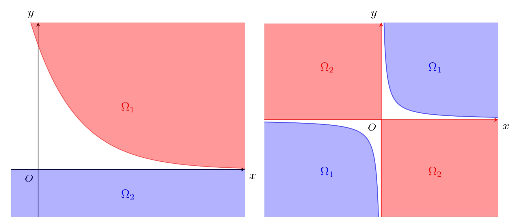
Figure 2: Example 2.6 (i) and (ii)

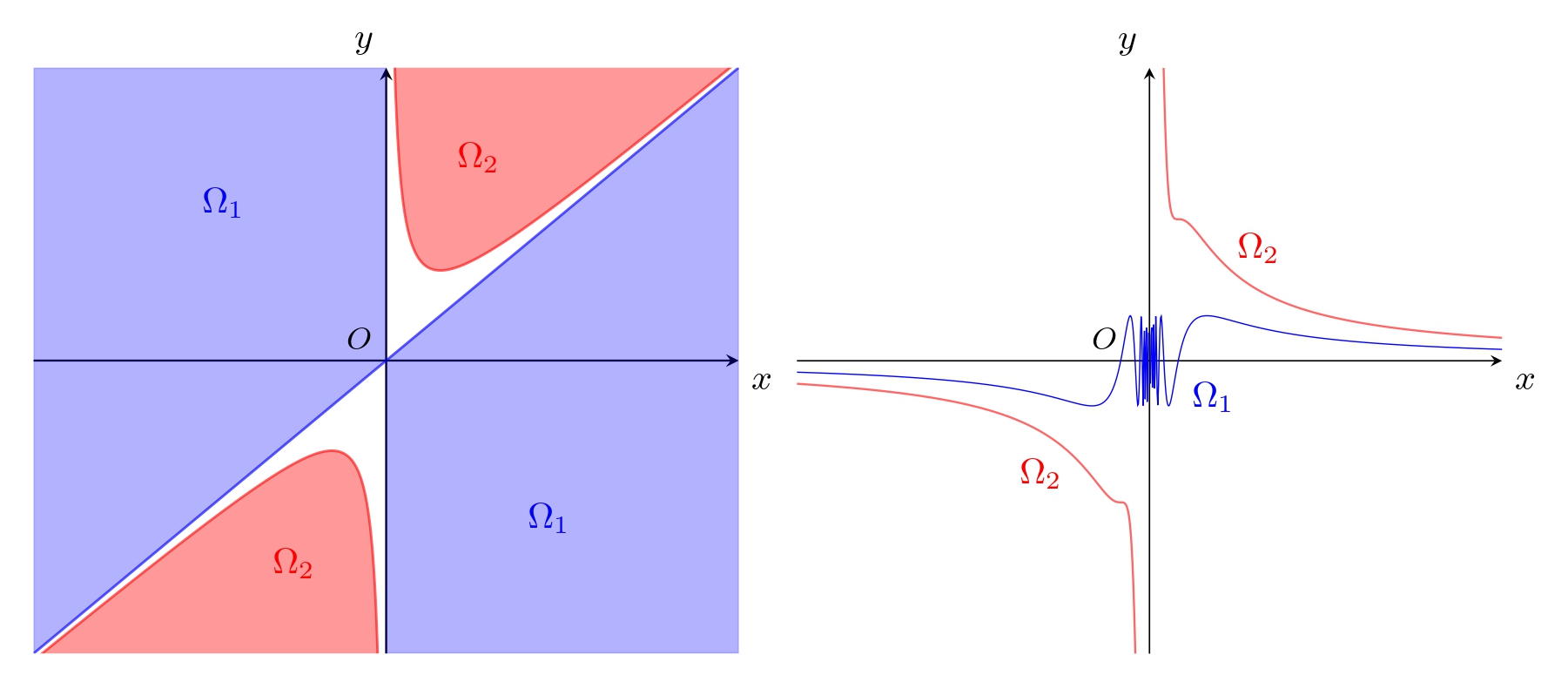
Figure 3: Example 2.6 (iii) and (iv)

In the convex case, the properties in Definition 2.1 admit simpler representations and are mostly equivalent.

Proposition 2.7 (Sequential extremality and stationarity: convex case).

Let $\Omega_{1},\ldots,\Omega_{n}$ be convex, $\{x_{i}^{k}\}\subset\Omega_{i}$ $(i=1,\ldots,n)$ and ${\rm diam}\,\{x_{1}^{k},\ldots,x_{n}^{k}\}\to 0$ as $k\to+\infty$. The following assertions are equivalent:

1. $\{\Omega_{1},\ldots,\Omega_{n}\}$ is extremal at $\{x^{k}_{i}\}$ $(i=1,\ldots,n)$ with any $\rho\in(0,+\infty)$;

2. $\{\Omega_{1},\ldots,\Omega_{n}\}$ is extremal at $\{x^{k}_{i}\}$ $(i=1,\ldots,n)$ with some $\rho\in(0,+\infty)$;

3. $\{\Omega_{1},\ldots,\Omega_{n}\}$ is stationary at $\{x^{k}_{i}\}$ $(i=1,\ldots,n)$;

4. for any $\varepsilon,\rho\in(0,+\infty)$, there exist an integer $k>\varepsilon^{-1}$, and a point $(a_{1},\ldots,a_{n})\in\varepsilon\mathbb{B}_{X^{n}}$ such that condition (13) is satisfied.

Proof.

The relations (iv) $\Leftrightarrow\$(i) $\Rightarrow$ (ii) $\Rightarrow$ (iii) are direct consequences of the definitions (cf. Remark 2.2 (iv)). We now prove implication (iii) $\Rightarrow$ (iv). Suppose that (iv) does not hold, i.e., there exist $\varepsilon,\rho\in(0,+\infty)$ such that

$$\bigcap_{i=1}^{n}(\Omega_{i}-x_{i}^{k}-a_{i})\cap(\rho\mathbb{B})\neq\emptyset$$ (14)

for all integers $k>\varepsilon^{-1}$ and points $(a_{1},\ldots,a_{n})\in\varepsilon\mathbb{B}_{X^{n}}$. Set $\varepsilon^{\prime}:=\min\{\varepsilon,\varepsilon/\rho\}$, and take arbitrarily an integer $k>\varepsilon^{\prime}{}^{-1}$, a positive $\rho^{\prime}<\varepsilon^{\prime}$ and a point $(a_{1}^{\prime},\ldots,a_{n}^{\prime})\in\varepsilon^{\prime}\rho^{\prime}\mathbb{B}_{X^{n}}$. Set $t:={\rho^{\prime}}/{\rho}$. Then $\left|\kern-1.07639pt\left|\kern-1.07639pt\left|(a_{1}^{\prime}/t,\ldots,a_{n}^{\prime}/t)\right|\kern-1.07639pt\right|\kern-1.07639pt\right|<\varepsilon^{\prime}\rho\leq\varepsilon$, and condition (14) implies the existence of an $x^{\prime}\in\rho\mathbb{B}$ such that $x^{\prime}+x_{i}^{k}+a_{i}^{\prime}/t\in\Omega_{i}$ $(i=1,\ldots,n)$. Then $tx^{\prime}\in\rho^{\prime}\mathbb{B}$ and $tx^{\prime}+x_{i}^{k}+a_{i}^{\prime}=t(x^{\prime}+x_{i}^{k}+a_{i}^{\prime}/t)+(1-t)x_{i}^{k}\in\Omega_{i}$ $(i=1,\ldots,n)$. Hence, $tx^{\prime}\in\bigcap_{i=1}^{n}(\Omega_{i}-x_{i}^{k}-a_{i}^{\prime})\cap(\rho^{\prime}\mathbb{B})$, and consequently, assertion (iii) does not hold. ∎

Proposition 2.8 (Sequential approximate stationarity: convex case).

Let $\Omega_{1},\ldots,\Omega_{n}$ be convex, and $\{x^{k}\}\subset X$.

1. $\{\Omega_{1},\ldots,\Omega_{n}\}$ is approximately stationary at $\{x^{k}\}$ if and only if for any $\varepsilon,\rho\in(0,+\infty)$, there exist an integer $k>\varepsilon^{-1}$, and points $(x_{1},\ldots,x_{n})\in\widehat{\Omega}\cap B_{\varepsilon}((x^{k},\ldots,x^{k})_{n})$ and $(a_{1},\ldots,a_{n})\in\varepsilon\mathbb{B}_{X^{n}}$ such that condition (6) is satisfied.

2. If $\{\Omega_{1},\ldots,\Omega_{n}\}$ is approximately stationary at $\{x^{k}\}$, then there exist a subsequence $x^{k_{j}}$, $j=1,2\ldots$, and sequences $\{x^{j}_{i}\}\subset\Omega_{i}$ $(i=1,\ldots,n)$ such that $x^{j}_{i}-x^{k_{j}}\to 0$ as $j\to+\infty$ $(i=1,\ldots,n)$, and $\{\Omega_{1},\ldots,\Omega_{n}\}$ is extremal at $\{x^{j}_{i}\}$ $(i=1,\ldots,n)$ with any $\rho>0$.

Proof.

1. The “if” part is obvious. We prove the “only if” part. Suppose that there exist $\varepsilon,\rho\in(0,+\infty)$ such that

   $$\bigcap_{i=1}^{n}(\Omega_{i}-x_{i}-a_{i})\cap(\rho\mathbb{B})\neq\emptyset$$ (15)

   for all integers $k>\varepsilon^{-1}$, and points $(x_{1},\ldots,x_{n})\in\widehat{\Omega}\cap B_{\varepsilon}((x^{k},\ldots,x^{k})_{n})$ and $(a_{1},\ldots,a_{n})\in\varepsilon\mathbb{B}_{X^{n}}$. Set $\varepsilon^{\prime}:=\min\{\varepsilon,\varepsilon/\rho\}$, and take arbitrarily an integer $k>\varepsilon^{\prime}{}^{-1}$, a positive $\rho^{\prime}<\varepsilon^{\prime}$ and points $(x_{1},\ldots,x_{n})\in\widehat{\Omega}\cap B_{\varepsilon^{\prime}}((x^{k},\ldots,x^{k})_{n})$ and $(a_{1}^{\prime},\ldots,a_{n}^{\prime})\in\varepsilon^{\prime}\rho^{\prime}\mathbb{B}_{X^{n}}$. Set $t:={\rho^{\prime}}/{\rho}$. Then $\left|\kern-1.07639pt\left|\kern-1.07639pt\left|(a_{1}^{\prime}/t,\ldots,a_{n}^{\prime}/t)\right|\kern-1.07639pt\right|\kern-1.07639pt\right|<\varepsilon^{\prime}\rho\leq\varepsilon$, and condition (15) implies the existence of an $x^{\prime}\in\rho\mathbb{B}$ such that $x^{\prime}+x_{i}+a_{i}^{\prime}/t\in\Omega_{i}$ $(i=1,\ldots,n)$. Then $tx^{\prime}\in\rho^{\prime}\mathbb{B}$ and $tx^{\prime}+x_{i}+a_{i}^{\prime}=t(x^{\prime}+x_{i}+a_{i}^{\prime}/t)+(1-t)x_{i}\in\Omega_{i}$ $(i=1,\ldots,n)$. Hence, $tx^{\prime}\in\bigcap_{i=1}^{n}(\Omega_{i}-x_{i}-a_{i}^{\prime})\cap(\rho^{\prime}\mathbb{B})$, and consequently, $\{\Omega_{1},\ldots,\Omega_{n}\}$ is not approximately stationary at $\{x^{k}\}$.

2. Suppose that $\{\Omega_{1},\ldots,\Omega_{n}\}$ is approximately stationary at $\{x^{k}\}$. Let $\varepsilon,\rho\in(0,+\infty)$. By (i), for any $j\in\mathbb{N}$, there exist an integer $k_{j}>j$, and points $(x_{1}^{j},\ldots,x_{n}^{j})\in\widehat{\Omega}\cap B_{1/j}((x^{k_{j}},\ldots,x^{k_{j}})_{n})$ and $(a_{1}^{j},\ldots,a_{n}^{j})\in(1/j)\mathbb{B}_{X^{n}}$ such that

   $$\bigcap_{i=1}^{n}(\Omega_{i}-x_{i}^{j}-a_{i}^{j})\cap(\rho\mathbb{B})=\emptyset.$$ (16)

   Thus, $k_{j}\to+\infty$, $x^{j}_{i}-x^{k_{j}}\to 0$ $(i=1,\ldots,n)$ and ${\rm diam}\,\{x_{1}^{j},\ldots,x_{n}^{j}\}\to 0$ as $j\to+\infty$. Take an integer $j>\varepsilon^{-1}$. Then $(a_{1}^{j},\ldots,a_{n}^{j})\in\varepsilon\mathbb{B}_{X^{n}}$ and, in view of (16), assertion (iv) in Proposition 2.7 is satisfied. The conclusion follows from Proposition 2.7.

∎

3 Sequential extremal principle

In this section, we study a quantitative version of the sequential approximate stationarity property in Definition 2.1 (iii) and prove dual necessary conditions in the form of generalized separation.

Definition 3.1 (Sequential approximate $\alpha$-stationarity).

Let $\alpha>0$. The collection $\{\Omega_{1},\ldots,\Omega_{n}\}$ is approximately $\alpha$-stationary at a sequence $\{x^{k}\}\subset X$ if, for any $\varepsilon>0$, there exist an integer $k>\varepsilon^{-1}$, a $\rho\in(0,\varepsilon)$, and points $(x_{1},\ldots,x_{n})\in\widehat{\Omega}\cap B_{\varepsilon}((x^{k},\ldots,x^{k})_{n})$ and $(a_{1},\ldots,a_{n})\in\alpha\rho\mathbb{B}_{X^{n}}$ such that condition (6) is satisfied.

Clearly, $\{\Omega_{1},\ldots,\Omega_{n}\}$ is approximately stationary at $\{x^{k}\}\subset X$ if it is approximately $\alpha$-stationary at $\{x^{k}\}$ for all $\alpha>0$. An analogue of Proposition 2.4 (iii) is true also for the sequential approximate $\alpha$-stationarity (for the definition of approximate $\alpha$-stationarity at a point we refer the reader to [12]).

As an application of the generalized separation Theorem 1.6, we prove dual necessary conditions for the sequential approximate $\alpha$-stationarity.

Theorem 3.2 (Sequential approximate $\alpha$-stationarity: generalized separation).

Let $X$ be Banach, $\Omega_{1},\ldots,\Omega_{n}$ be closed, and $\alpha>0$. Suppose that $\{\Omega_{1},\ldots,\Omega_{n}\}$ is approximately $\alpha$-stationary at $\{x^{k}\}\subset X$. The following assertions hold true:

1. for any $\varepsilon>0$, $\beta>\alpha$ and $\tau\in(0,1)$, there exist an integer $k>\varepsilon^{-1}$, and points $(a_{1},\ldots,a_{n})\in\varepsilon\mathbb{B}_{X^{n}}$, $\hat{x}:=(x_{1},\ldots,x_{n}),\hat{x}^{\prime}:=(x^{\prime}_{1},\ldots,x^{\prime}_{n})\in\widehat{\Omega}\cap B_{\varepsilon}((x^{k},\ldots,x^{k})_{n})$, $x_{0}\in\varepsilon\mathbb{B}_{X}$ and $\hat{x}^{*}:=(x_{1}^{*},\ldots,x_{n}^{*})\in N^{C}_{\widehat{\Omega}}(\hat{x})$ such that

   $$\Big{\|}{\sum_{i=1}^{n}x_{i}^{*}}\Big{\|}<\beta,\quad\left|\kern-1.07639pt\left|\kern-1.07639pt\left|\hat{x}^{*}\right|\kern-1.07639pt\right|\kern-1.07639pt\right|=1,$$ (17)

   $$\left\langle\hat{x}^{*},(x_{0}\ldots,x_{0})_{n}+\hat{a}+\hat{x}^{\prime}-\hat{x}\right\rangle>\tau\left|\kern-1.07639pt\left|\kern-1.07639pt\left|(x_{0}\ldots,x_{0})_{n}+\hat{a}+\hat{x}^{\prime}-\hat{x}\right|\kern-1.07639pt\right|\kern-1.07639pt\right|;$$ (18)

2. if $X$ is Asplund, then $N^{C}$ in (i) can be replaced by $N^{F}$.

Proof.

Let $\varepsilon>0$, $\beta>\alpha$, $\tau\in(0,1)$. It is easy to check that the second inequality in (5) implies the next compatibility condition for the dual norms (with the same $\kappa_{2}>0$):

$$\sum_{i=1}^{n}\|u_{i}^{*}\|\leq\kappa_{2}\left|\kern-1.07639pt\left|\kern-1.07639pt\left|(u_{1}^{*},\ldots,u_{n}^{*})\right|\kern-1.07639pt\right|\kern-1.07639pt\right|\quad\text{for all}\;\;u_{1}^{*},\ldots,u_{n}^{*}\in X^{*}.$$ (19)

Choose a number $\xi>0$ so that

$$2\xi<1-\tau,\quad\xi^{2}<\varepsilon,\quad\alpha\xi<\varepsilon\and\frac{\alpha+\kappa_{2}\xi}{1-\xi}<\beta.$$ (20)

By Definition 3.1, there exist a $\rho\in(0,\xi^{2})$, an integer $k>\xi^{-2}$, and points $\hat{a}:=(a_{1},\ldots,a_{n})\in\alpha\rho\mathbb{B}_{X^{n}}$ and $\hat{x}^{\prime}:=(x_{1}^{\prime},\ldots,x_{n}^{\prime})\in\widehat{\Omega}\cap B_{\xi^{2}}((x^{k},\ldots,x^{k})_{n})$ such that $\bigcap_{i=1}^{n}(\Omega_{i}-x_{i}^{\prime}-a_{i})\cap(\rho\mathbb{B})=\emptyset$.

Choose a $\rho^{\prime}\in(\left|\kern-1.07639pt\left|\kern-1.07639pt\left|\hat{a}\right|\kern-1.07639pt\right|\kern-1.07639pt\right|/\alpha,\rho)$, and set $\varepsilon^{\prime}:=\alpha\rho^{\prime}$ and $\delta:=\alpha\sqrt{\rho^{\prime}}$. Then $\bigcap_{i=1}^{n}(\Omega_{i}-x_{i}^{\prime}-a_{i})\cap(\rho^{\prime}\overline{\mathbb{B}})=\emptyset$ and $\left|\kern-1.07639pt\left|\kern-1.07639pt\left|\hat{a}\right|\kern-1.07639pt\right|\kern-1.07639pt\right|<\varepsilon^{\prime}$. By Theorem 1.6 (i), there exist points $\hat{x}:=(x_{1},\ldots,x_{n})\in\widehat{\Omega}\cap B_{\delta}(\hat{x}^{\prime})$, $x_{0}\in\rho^{\prime}\mathbb{B}$ and $\hat{x}^{\prime*}:=(x_{1}^{\prime*},\ldots,x_{n}^{\prime*})\in(X^{*})^{n}$ such that $\left|\kern-1.07639pt\left|\kern-1.07639pt\left|\hat{x}^{\prime*}\right|\kern-1.07639pt\right|\kern-1.07639pt\right|=1$ and

$$\delta d\left(\hat{x}^{\prime*},N^{C}_{\widehat{\Omega}}(\hat{x})\right)+\rho^{\prime}\Big{\|}\sum_{i=1}^{n}x_{i}^{\prime*}\Big{\|}<\varepsilon^{\prime},$$ (21)

$$\left\langle\hat{x}^{\prime*},(x_{0}\ldots,x_{0})_{n}+\hat{a}+\hat{x}^{\prime}-\hat{x}\right\rangle=\left|\kern-1.07639pt\left|\kern-1.07639pt\left|(x_{0}\ldots,x_{0})_{n}+\hat{a}+\hat{x}^{\prime}-\hat{x}\right|\kern-1.07639pt\right|\kern-1.07639pt\right|.$$ (22)

Thus, $k>\xi^{-2}>\varepsilon^{-1}$, $\left|\kern-1.07639pt\left|\kern-1.07639pt\left|\hat{a}\right|\kern-1.07639pt\right|\kern-1.07639pt\right|<\alpha\xi^{2}<\alpha\xi<\varepsilon$, $\left|\kern-1.07639pt\left|\kern-1.07639pt\left|(x_{1}-x^{k},\ldots,x_{n}-x^{k})\right|\kern-1.07639pt\right|\kern-1.07639pt\right|<\delta<\alpha\xi<\varepsilon$ and $\|x_{0}\|<\rho^{\prime}<\xi^{2}<\varepsilon$. By (21),

$$d\left(\hat{x}^{\prime*},N^{C}_{\widehat{\Omega}}(\hat{x})\right)<\frac{\varepsilon^{\prime}}{\delta}=\frac{\alpha\rho^{\prime}}{\alpha\sqrt{\rho^{\prime}}}<\xi,\quad\Big{\|}\sum_{i=1}^{n}x_{i}^{\prime*}\Big{\|}<\frac{\varepsilon^{\prime}}{\rho^{\prime}}=\alpha.$$

Thus, there is a $\hat{z}^{*}:=(z_{1}^{*},\ldots,z_{n}^{*})\in N^{C}_{\widehat{\Omega}}(\hat{x})$ such that $\left|\kern-1.07639pt\left|\kern-1.07639pt\left|\hat{x}^{\prime*}-\hat{z}^{*}\right|\kern-1.07639pt\right|\kern-1.07639pt\right|<\xi$, and consequently, ${0<1-\xi}<\left|\kern-1.07639pt\left|\kern-1.07639pt\left|\hat{z}^{*}\right|\kern-1.07639pt\right|\kern-1.07639pt\right|<1+\xi$. By (19),

$$\Big{\|}\sum_{i=1}^{n}z_{i}^{*}\Big{\|}\leq\Big{\|}\sum_{i=1}^{n}x_{i}^{\prime*}\Big{\|}+\sum_{i=1}^{n}\|z^{*}_{i}-x_{i}^{\prime*}\|<\alpha+\kappa_{2}\xi.$$

Set $\hat{x}^{*}:=(x_{1}^{*},\ldots,x_{n}^{*}):=\dfrac{\hat{z}^{*}}{\left|\kern-1.07639pt\left|\kern-1.07639pt\left|\hat{z}^{*}\right|\kern-1.07639pt\right|\kern-1.07639pt\right|}$. Then, $\hat{x}^{*}\in N^{C}_{\widehat{\Omega}}(\hat{x})$, $\left|\kern-1.07639pt\left|\kern-1.07639pt\left|\hat{x}^{*}\right|\kern-1.07639pt\right|\kern-1.07639pt\right|=1$ and, in view of the last inequality in (20),

$$\Big{\|}\sum_{i=1}^{n}x_{i}^{*}\Big{\|}<\frac{\alpha+\kappa_{2}\xi}{1-\xi}<\beta.$$

Hence, conditions (17) are satisfied. Moreover,

$$\left|\kern-1.07639pt\left|\kern-1.07639pt\left|\hat{x}^{*}-\hat{x}^{\prime*}\right|\kern-1.07639pt\right|\kern-1.07639pt\right| \leq\left|\kern-1.07639pt\left|\kern-1.07639pt\left|\frac{\hat{z}^{*}}{\left|\kern-1.07639pt\left|\kern-1.07639pt\left|\hat{z}^{*}\right|\kern-1.07639pt\right|\kern-1.07639pt\right|^{*}}-\hat{z}^{*}\right|\kern-1.07639pt\right|\kern-1.07639pt\right|+\left|\kern-1.07639pt\left|\kern-1.07639pt\left|\hat{z}^{*}-\hat{x}^{\prime*}\right|\kern-1.07639pt\right|\kern-1.07639pt\right|<\left|\left|\kern-1.07639pt\left|\kern-1.07639pt\left|\hat{z}^{*}\right|\kern-1.07639pt\right|\kern-1.07639pt\right|^{*}-1\right|+\xi<2\xi.$$

Denote $m:=\left|\kern-1.07639pt\left|\kern-1.07639pt\left|(x_{0}\ldots,x_{0})_{n}+\hat{a}+\hat{x}^{\prime}-\hat{x}\right|\kern-1.07639pt\right|\kern-1.07639pt\right|$. Condition (18) follows from (20), (22), and the last estimate:

$$\left\langle\hat{x}^{*},(x_{0}\ldots,x_{0})_{n}+\hat{a}+\hat{x}^{\prime}-\hat{x}\right\rangle>\left\langle\hat{x}^{\prime*},(x_{0}\ldots,x_{0})_{n}+\hat{a}+\hat{x}^{\prime}-\hat{x}\right\rangle-2\xi m\\ =(1-2\xi)m>\tau m.$$ (23)

Suppose $X$ is Asplund. Let $\hat{\tau}\in(\tau+2\xi,1)$. Application of Theorem 1.6 (ii) with $\hat{\tau}$ in place of $\tau$ in the above proof justifies conditions (17) with $\hat{x}^{*}\in N^{F}_{\widehat{\Omega}}(\hat{x})$, while the factor $1-2\xi$ in (23) needs to be replaced by $\hat{\tau}-2\xi$ leading to the same estimate. This again proves (18). ∎

Corollary 3.3 (Sequential approximate stationarity: generalized separation).

Let $X$ be Banach, and $\Omega_{1},\ldots,\Omega_{n}$ be closed. Suppose that $\{\Omega_{1},\ldots,\Omega_{n}\}$ is approximately stationary at $\{x^{k}\}\subset X$. The following assertions hold true:

1. for any $\varepsilon>0$ and $\tau\in(0,1)$, there exist an integer $k>\varepsilon^{-1}$, and points $(a_{1},\ldots,a_{n})\in\varepsilon\mathbb{B}_{X^{n}}$, $\hat{x}:=(x_{1},\ldots,x_{n}),\hat{x}^{\prime}:=(x^{\prime}_{1},\ldots,x^{\prime}_{n})\in\widehat{\Omega}\cap B_{\varepsilon}((x^{k},\ldots,x^{k})_{n})$, $x_{0}\in\varepsilon\mathbb{B}_{X}$ and $\hat{x}^{*}:=(x_{1}^{*},\ldots,x_{n}^{*})\in N^{C}_{\widehat{\Omega}}(\hat{x})$ such that conditions (7) and (18) are satisfied;

2. for any $\varepsilon>0$, there exist an integer $k>\varepsilon^{-1}$, and points $\hat{x}:=(x_{1},\ldots,x_{n})\in\widehat{\Omega}\cap B_{\varepsilon}((x^{k},\ldots,x^{k})_{n})$ and $\hat{x}^{*}:=(x_{1}^{*},\ldots,x_{n}^{*})\in N^{C}_{\widehat{\Omega}}(\hat{x})$ such that conditions (7) are satisfied;

3. if $X$ is Asplund, then $N^{C}$ in (i) and (ii) can be replaced by $N^{F}$.

The necessary conditions in Corollary 3.3 are applicable (with obvious amendments) to the stationarity and extremality properties in Definition 2.1. In particular, we can formulate a result generalizing and extending the conventional extremal principle in Theorem 1.2.

Corollary 3.4 (Sequential extremal principle).

Let $X$ be Banach, and $\Omega_{1},\ldots,\Omega_{n}$ be closed. Suppose that $\{\Omega_{1},\ldots,\Omega_{n}\}$ is extremal at $\{x_{i}^{k}\}\subset\Omega_{i}$ $(i=1,\ldots,n)$. The following assertions hold true:

1. for any $\varepsilon>0$ and $\tau\in(0,1)$, there exist an integer $k>\varepsilon^{-1}$, and points $(a_{1},\ldots,a_{n})\in\varepsilon\mathbb{B}_{X^{n}}$, $\hat{x}:=(x_{1},\ldots,x_{n}),\hat{x}^{\prime}:=(x^{\prime}_{1},\ldots,x^{\prime}_{n})\in\widehat{\Omega}\cap B_{\varepsilon}(x_{1}^{k},\ldots,x_{n}^{k})$, $x_{0}\in\varepsilon\mathbb{B}_{X}$ and $\hat{x}^{*}:=(x_{1}^{*},\ldots,x_{n}^{*})\in N^{C}_{\widehat{\Omega}}(\hat{x})$ such that conditions (7) and (18) are satisfied;

2. for any $\varepsilon>0$, there exist an integer $k>\varepsilon^{-1}$, and points $\hat{x}:=(x_{1},\ldots,x_{n})\in\widehat{\Omega}\cap B_{\varepsilon}(x_{1}^{k},\ldots,x_{n}^{k})$ and $\hat{x}^{*}:=(x_{1}^{*},\ldots,x_{n}^{*})\in N^{C}_{\widehat{\Omega}}(\hat{x})$ such that conditions (7) are satisfied;

3. if $X$ is Asplund, then $N^{C}$ in (i) and (ii) can be replaced by $N^{F}$.

Proof.

The statement is a consequence of Corollary 3.3 in view of Remark 2.2 (iv) and the fact that ${\rm diam}\,\{x_{1}^{k},\ldots,x_{n}^{k}\}\to 0$ as $k\to+\infty$ (see Definition 2.1 (i)). ∎

Remark 3.5.

1. The second assertions in Corollaries 3.3 and 3.4 are simplified versions of the first ones. They corresponds to dropping inequality (18) together with the variables involved only in this condition. A similar simplification can be made in assertion (i) of Theorem 3.2.

2. Imposing certain sequential normal compactness assumptions (which are automatically satisfied in finite dimensions), one can formulate limiting versions of Theorem 3.2 and Corollary 3.3 in terms of certain types of limiting normal cones. This remark applies also to the statements in the rest of the paper.

The Asplund space assertion (ii) in Theorem 3.2 can be partially reversed; cf., e.g., [12].

Theorem 3.6 (Sequential generalized separation in Asplund spaces).

Let $\{x^{k}\}\subset X$, $\alpha>0$ and $\beta>0$. Consider the following assertions:

1. $\{\Omega_{1},\ldots,\Omega_{n}\}$ is approximately $\alpha$-stationary at $\{x^{k}\}$;

2. for any $\varepsilon>0$ and $\tau\in(0,1)$, there exist an integer $k>\varepsilon^{-1}$, and points $(a_{1},\ldots,a_{n})\in\varepsilon\mathbb{B}_{X^{n}}$, $\hat{x}:=(x_{1},\ldots,x_{n}),\hat{x}^{\prime}:=(x^{\prime}_{1},\ldots,x^{\prime}_{n})\in\widehat{\Omega}\cap B_{\varepsilon}((x^{k},\ldots,x^{k})_{n})$, $x_{0}\in\varepsilon\mathbb{B}_{X}$ and $\hat{x}^{*}:=(x_{1}^{*},\ldots,x_{n}^{*})\in N^{C}_{\widehat{\Omega}}(\hat{x})$ such that conditions (17) and (18) are satisfied;

3. for any $\varepsilon>0$, there exist an integer $k>\varepsilon^{-1}$, and points $\hat{x}:=(x_{1},\ldots,x_{n})\in\widehat{\Omega}\cap B_{\varepsilon}((x^{k},\ldots,x^{k})_{n})$ and $\hat{x}^{*}:=(x_{1}^{*},\ldots,x_{n}^{*})\in N^{F}_{\widehat{\Omega}}(\hat{x})$ such that conditions (17) are satisfied.

The following relations hold true:

1. (ii) $\Rightarrow\$(iii);

2. if $X$ is Asplund, $\Omega_{1},\ldots,\Omega_{n}$ are closed, and $\beta>\alpha$, then (i) $\Rightarrow\$(ii);

3. if $\alpha>\beta$, then (iii) $\Rightarrow$ (i).

Proof.

The implication in (a) is straightforward as (iii) is a simplified version of (ii); see Remark 3.5 (i). The implication in (b) is a direct consequence of Theorem 3.2 (ii). We now prove the implication in (c).

Suppose that the second inequality in (5) is satisfied with some $\kappa_{2}>0$, assertion (iii) holds true, and $\alpha>\beta$. Let $\varepsilon>0$. Then, there exist an integer $k>\varepsilon^{-1}$, and points $\hat{x}:=(x_{1},\ldots,x_{n})\in\widehat{\Omega}\cap B_{\varepsilon}((x^{k},\ldots,x^{k})_{n})$ and $\hat{x}^{*}:=(x_{1}^{*},\ldots,x_{n}^{*})\in N^{F}_{\widehat{\Omega}}(\hat{x})$ such that conditions (17) are satisfied.

Choose a $\xi\in(0,\alpha-\beta)$. Thus, $\xi^{\prime}:=\alpha-\beta-\xi>0$. By the definition of Fréchet normal cone, there is a $\rho\in(0,\varepsilon)$ such that

$$\langle\hat{x}^{*},\hat{\omega}-\hat{x}\rangle\leq\dfrac{\xi}{\kappa_{2}+\alpha}\left|\kern-1.07639pt\left|\kern-1.07639pt\left|\hat{\omega}-\hat{x}\right|\kern-1.07639pt\right|\kern-1.07639pt\right|<\xi\rho\;\;\text{for all}\;\;\hat{\omega}\in\widehat{\Omega}\;\;\text{with}\;\;\left|\kern-1.07639pt\left|\kern-1.07639pt\left|\hat{\omega}-\hat{x}\right|\kern-1.07639pt\right|\kern-1.07639pt\right|<(\kappa_{2}+\alpha)\rho.$$ (24)

By the equality in (17), one can choose an $\hat{a}:=(a_{1},\ldots,a_{n})\in X^{n}$ such that

$$\left|\kern-1.07639pt\left|\kern-1.07639pt\left|\hat{a}\right|\kern-1.07639pt\right|\kern-1.07639pt\right|<\alpha\rho\;\;\text{and}\;\;\langle\hat{x}^{*},\hat{a}\rangle>(\alpha-\xi^{\prime})\rho=(\beta+\xi)\rho.$$ (25)

We now show that $\bigcap_{i=1}^{n}(\Omega_{i}-x_{i}-a_{i})\cap(\rho\mathbb{B})=\emptyset$. Indeed, suppose that $\omega_{i}-x_{i}-a_{i}=x_{0}$ for some $x_{0}\in\rho\mathbb{B}$ and $\hat{\omega}:=(\omega_{1},\ldots,\omega_{n})\in\widehat{\Omega}$, and all $i=1,\ldots,n$. Then, in view of (5) and the first inequality in (25),

$$\left|\kern-1.07639pt\left|\kern-1.07639pt\left|\hat{\omega}-\hat{x}\right|\kern-1.07639pt\right|\kern-1.07639pt\right|\leq\left|\kern-1.07639pt\left|\kern-1.07639pt\left|(x_{0},\ldots,x_{0})_{n}\right|\kern-1.07639pt\right|\kern-1.07639pt\right|+\left|\kern-1.07639pt\left|\kern-1.07639pt\left|\hat{a}\right|\kern-1.07639pt\right|\kern-1.07639pt\right|\leq\kappa_{2}\|x_{0}\|+\left|\kern-1.07639pt\left|\kern-1.07639pt\left|\hat{a}\right|\kern-1.07639pt\right|\kern-1.07639pt\right|<(\kappa_{2}+\alpha)\rho,$$

and, by (24), $\left\langle\hat{x}^{*},\hat{\omega}-\hat{x}\right\rangle<\xi\rho$. Combining this with the second inequality in (25), we obtain

$$\Big{\langle}\sum_{i=1}^{n}x^{*}_{i},x_{0}\Big{\rangle}=\langle\hat{x}^{*},(x_{0},\ldots,x_{0})_{n}\rangle=\langle\hat{x}^{*},\hat{\omega}-\hat{x}\rangle-\langle\hat{x}^{*},\hat{a}\rangle<-\beta\rho.$$

On the other hand, by the inequality in (17), $\langle\sum_{i=1}^{n}x^{*}_{i},x_{0}\rangle>-\beta\rho,$ a contradiction. Hence, condition (6) is satisfied, and $\{\Omega_{1},\ldots,\Omega_{n}\}$ is approximate $\alpha$-stationary at $\{x^{k}\}$. ∎

The next corollary generalizes and improves the extended extremal principle in Theorem 1.4.

Corollary 3.7 (Sequential extended extremal principle).

Let $X$ be Asplund, $\Omega_{1},\ldots,\Omega_{n}$ be closed, and $\{x^{k}\}\subset X$. The following assertions are equivalent:

1. $\{\Omega_{1},\ldots,\Omega_{n}\}$ is approximately stationary at $\bar{x}$;

2. for any $\varepsilon>0$ and $\tau\in(0,1)$, there exist an integer $k>\varepsilon^{-1}$, and points $\hat{x}:=(x_{1},\ldots,x_{n}),\hat{x}^{\prime}:=(x^{\prime}_{1},\ldots,x^{\prime}_{n})\in\widehat{\Omega}\cap B_{\varepsilon}((x^{k},\ldots,x^{k})_{n})$, $x_{0}\in\varepsilon\mathbb{B}_{X}$, $\hat{x}^{*}:=(x_{1}^{*},\ldots,x_{n}^{*})\in N^{F}_{\widehat{\Omega}}(\hat{x})$, and $(a_{1},\ldots,a_{n})\in\varepsilon\mathbb{B}_{X^{n}}$ such that conditions (7) and (18) are satisfied;

3. for any $\varepsilon>0$, there exist an integer $k>\varepsilon^{-1}$, and points $\hat{x}:=(x_{1},\ldots,x_{n})\in\widehat{\Omega}\cap B_{\varepsilon}((x^{k},\ldots,x^{k})_{n})$ and $\hat{x}^{*}:=(x_{1}^{*},\ldots,x_{n}^{*})\in N^{F}_{\widehat{\Omega}}(\hat{x})$ such that conditions (7) are satisfied.

Remark 3.8.

Implications (ii) $\Rightarrow\$(iii) $\Rightarrow\$(i) in Corollary 3.7 are true in the setting of an arbitrary normed vector space and not necessary closed sets $\Omega_{1},\ldots,\Omega_{n}$. The Asplund property of the space and closedness of the sets are only needed for implication (i) $\Rightarrow\$(ii) which is a consequence of Theorem 3.6 (b).

Reversing the conditions in Definition 3.1, we arrive at extensions of the transversality properties discussed in [19, 26, 27].

Definition 3.9 (Sequential transversality).

1. Let $\alpha>0$. The collection $\{\Omega_{1},\ldots,\Omega_{n}\}$ is $\alpha$-transversal at $\{x^{k}\}\subset X$ if there is an $\varepsilon>0$ such that condition (15) is satisfied for all $\rho\in(0,\varepsilon)$, integers $k>\varepsilon^{-1}$, and points $(x_{1},\ldots,x_{n})\in\widehat{\Omega}\cap B_{\varepsilon}((x^{k},\ldots,x^{k})_{n})$ and $(a_{1},\ldots,a_{n})\in\alpha\rho\mathbb{B}_{X^{n}}$.

2. The collection $\{\Omega_{1},\ldots,\Omega_{n}\}$ is transversal at $\{x^{k}\}\subset X$ if it is $\alpha$-transversal at $\{x^{k}\}$ for some $\alpha>0$.

The statements of Theorem 3.2 and its corollaries can also be easily “reversed” to produce a dual characterization of transversality. For instance, Corollary 3.7 leads to the following statement.

Corollary 3.10 (Sequential transversality: dual characterization).

Let $X$ be Asplund, and $\Omega_{1},\ldots,\Omega_{n}$ be closed. The collection $\{\Omega_{1},\ldots,\Omega_{n}\}$ is transversal at $\{x^{k}\}\subset X$ if and only if there is an $\varepsilon>0$ such that $\left\|\sum_{i=1}^{n}x^{*}_{i}\right\|\geq\varepsilon$ for all integers $k>\varepsilon^{-1}$, and points $\hat{x}:=(x_{1},\ldots,x_{n})\in\widehat{\Omega}\cap B_{\varepsilon}((x^{k},\ldots,x^{k})_{n})$ and $\hat{x}^{*}:=(x_{1}^{*},\ldots,x_{n}^{*})\in N^{F}_{\widehat{\Omega}}(\hat{x})$ with $\left|\kern-1.07639pt\left|\kern-1.07639pt\left|\hat{x}^{*}\right|\kern-1.07639pt\right|\kern-1.07639pt\right|=1$.

Remark 3.11.

The “only if” part of Corollary 3.10 is true in the setting of an arbitrary normed vector space and not necessary closed sets $\Omega_{1},\ldots,\Omega_{n}$; cf. Remark 3.8.

4 Sequential minimality and stationarity

To illustrate the model studied in the previous sections, we consider the following constrained optimization problem:

$$\text{minimize }\;f(x)\quad\text{subject to }\;x\in\Omega, {P}$$ ()

where $\Omega$ is a nonempty subset of a normed vector space $X$. Below, we recall the conventional definition of a minimizing sequence and introduce its localized version.

Definition 4.1 (Minimizing sequence).

1. A sequence $\{x^{k}\}\subset\Omega$ is minimizing for problem (${P}$) if $f(x^{k})\to\inf_{\Omega}f$.

2. A sequence $\{x^{k}\}\subset\Omega$ is minimizing for problem (${P}$) at level $\mu_{0}\in\mathbb{R}$ if $f(x^{k})\to\mu_{0}$ as $k\to+\infty$, and there exist a $\rho\in(0,+\infty]$ and a $k_{0}>0$ such that

   $$f(x)\geq\mu_{0}\;\;\text{for all}\;\;x\in\Omega\cap B_{\rho}(x^{k})\;\;\text{and all integers}\;\;k>k_{0}.$$ (26)

The assertions in the next proposition are immediate consequences of the definitions. They show, in particular, that the properties in Definition 4.1 are not too different.

Proposition 4.2.

Let $\{x^{k}\}\subset\Omega$ and $\mu_{0}\in\mathbb{R}$. The following assertions hold true:

1. if $\{x^{k}\}$ is minimizing for problem (${P}$) at level $\mu_{0}$ with some $\rho\in(0,+\infty]$, and $x^{k}=\bar{x}$ for all $k\in\mathbb{N}$, then $f(\bar{x})=\mu_{0}=\min_{\Omega\cap B_{\rho}(\bar{x})}f$;

2. if $\{x^{k}\}$ is minimizing for problem (${P}$) and $\inf_{\Omega}f\in\mathbb{R}$, then it is minimizing for problem (${P}$) at level $\inf_{\Omega}f$ with $\rho=+\infty$;

3. if $\{x^{k}\}$ is minimizing for problem (${P}$) at level $\mu_{0}$, then $\mu_{0}\geq\inf_{\Omega}f$;

4. if $\{x^{k}\}$ is minimizing for problem (${P}$) at level $\mu_{0}$ with $\rho=+\infty$, then it is minimizing for problem (${P}$) and $\mu_{0}=\inf_{\Omega}f$.

Corollary 4.3.

Let $\inf_{\Omega}f\in\mathbb{R}$. A sequence $\{x^{k}\}\subset\Omega$ is minimizing for problem (${P}$) if and only if it is minimizing for problem (${P}$) at level $\inf_{\Omega}f$ with $\rho=+\infty$.

Example 4.4 (Minimizing sequence at level $0$).

Let $\Omega=\mathbb{R}$, $f(x)=1/x$ for all $x\neq 0$ and $f(0)=+\infty$; see Figure 4. Any sequence of real numbers $x_{k}\to+\infty$ is minimizing for (${P}$) at level $0$. Observe that it is not a minimizing sequence.

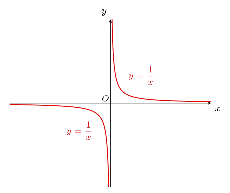
Figure 4: Example 4.4

The stationarity properties in the next definition are counterparts of the corresponding ones in Definition 2.1.

Definition 4.5 (Stationarity).

1. A sequence $\{x^{k}\}\subset\Omega$ is firmly $\inf$-stationary for problem (${P}$) at level $\mu_{0}\in\mathbb{R}$ if $f(x^{k})\to\mu_{0}$ as $k\to+\infty$, and there is a $\rho\in(0,+\infty]$ such that

   $$\limsup_{k\to+\infty}\inf_{\Omega\cap B_{\rho}(x^{k})}f=\mu_{0}.$$ (27)

2. A sequence $\{x^{k}\}\subset\Omega$ is $\inf$-stationary for problem (${P}$) at level $\mu_{0}\in\mathbb{R}$ if $f(x^{k})\to\mu_{0}$ as $k\to+\infty$, and

   $$\limsup_{k\to+\infty,\,\rho\downarrow 0}\frac{\inf_{\Omega\cap B_{\rho}(x^{k})}f-f(x^{k})}{\rho}=0.$$ (28)

3. A sequence $\{x^{k}\}\subset X$ is approximately $\inf$-stationary for problem (${P}$) at level $\mu_{0}\in\mathbb{R}$ if

   $$\limsup_{\begin{subarray}{c}k\to+\infty,\,\rho\downarrow 0\\ u^{k}\in\Omega,\,u^{k}-x^{k}\to 0,\,f(u^{k})\to\mu_{0}\end{subarray}}\frac{\inf_{\Omega\cap B_{\rho}(u^{k})}f-f(u^{k})}{\rho}=0.$$ (29)

Remark 4.6.

1. If $x^{k}=\bar{x}$ for all $k\in\mathbb{N}$, the property in part (i) of Definition 4.5 coincides with that in Definition 4.1 (ii), and $f(\bar{x})=\mu_{0}=\min_{\Omega\cap B_{\rho}(\bar{x})}f$. If, additionally, $\Omega=X$, the properties in parts (ii) and (iii) reduce to the, respectively, $\inf$-stationarity and approximate $\inf$-stationarity (weak $\inf$-stationarity) studied in [28, 21].

2. The property in Definition 4.1 (ii) implies firm stationarity in Definition 4.5 (i), and (i) $\Rightarrow$ (ii) $\Rightarrow$ (iii) in Definition 4.5. The converse implications are not true in general. See [28, Examples 1–4] for the case $x^{k}:=\bar{x}$ $(k\in\mathbb{N})$. The sequential case is illustrated in Examples 4.7, 4.8 and 4.9 below.

Example 4.7 (firm inf-stationarity).

Let $\Omega=\mathbb{R}$, $f(x)=1/x$ for all $x\neq 0$ and $f(0)=+\infty$ (see Example 4.4). For the sequence $x_{k}:=-k$ $(k\in\mathbb{N})$, we have $f(x^{k})\to 0$ as $k\to+\infty$, but the sequence is not minimizing for (${P}$) at level $0$ as $f(x)<0$ for all $x<0$. For $\rho:=1$,

$$\limsup_{k\to+\infty}\inf_{\Omega\cap B_{\rho}(x^{k})}f=\lim_{k\to+\infty}\frac{1}{-k+1}=0.$$

By Definition 4.5 (i), $\{x^{k}\}$ is firmly $\inf$-stationary for (${P}$) at level $0$.

Example 4.8 (inf-stationarity).

Let $\Omega=\mathbb{R}$, $f(x)=1/|x|-(x-k)^{2}$ for all $x\in[k-1/2,k+1/2)$, $k=\pm 1,\pm 2,\ldots$ and $f(x)=7/4$ for all $x\in(-1/2,1/2)$; see Figure 5. For $x_{k}:=k$, we have $f(x^{k})=1/k\to 0$ as $k\to+\infty$, and for any $\rho>0$,

$$\inf_{B_{\rho}(x^{k})}f=\frac{1}{k+\rho}-\min\Big{\{}\rho^{2},\frac{1}{4}\Big{\}}\and\limsup_{k\to+\infty}\inf_{B_{\rho}(x^{k})}f=-\min\Big{\{}\rho^{2},\frac{1}{4}\Big{\}}<0.$$

By Definition 4.5 (i), $\{x^{k}\}$ is not firmly $\inf$-stationary for (${P}$) at level 0. At the same time,

$$\limsup_{\begin{subarray}{c}k\to+\infty\\ \rho\downarrow 0\end{subarray}}\frac{\inf_{B_{\rho}(x^{k})}f-f(x^{k})}{\rho}= \lim_{\begin{subarray}{c}k\to+\infty\\ \rho\downarrow 0\end{subarray}}\frac{\frac{1}{k+\rho}-\rho^{2}-\frac{1}{k}}{\rho}=-\lim_{\begin{subarray}{c}k\to+\infty\\ \rho\downarrow 0\end{subarray}}\Big{(}\frac{1}{k(k+\rho)}+\rho\Big{)}=0.$$

By Definition 4.5 (ii), $\{x^{k}\}$ is $\inf$-stationary for (${P}$) at level 0.

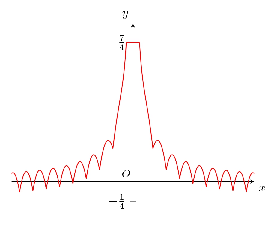
Figure 5: Example 4.8

Example 4.9 (approximate inf-stationarity).

Let $\Omega=\mathbb{R}$. Consider a continuous function

$$f(x)=\begin{cases}(x-2k\pi^{-1})\sin\frac{1}{x-{2k}\pi^{-1}}&\text{if }0<|x-{2k}\pi^{-1}|\leq\pi^{-1},\;\;k=0,\pm 1,\pm 2,\ldots,\\ 0&\text{otherwise};\end{cases}$$

see Figure 6. For the sequence $x^{k}:={2k}\pi^{-1}$ $(k\in\mathbb{N})$, we have $f(x^{k})=0$ for all $k\in\mathbb{N}$, but the sequence is not inf-stationary for (${P}$) at level $0$. Indeed, for any $k\in\mathbb{N}$ and $\rho\in(0,\pi^{-1})$, set $j:=\lceil\frac{1}{2\pi\rho}+\frac{1}{4}\rceil$, ${\delta}:=\frac{2}{(4j-1)\pi}$ and $x^{\prime k}:=x^{k}+\delta$. Then $\frac{1}{2\pi+{\rho}^{-1}}<\delta\leq\rho$ and $f(x^{\prime k})=\delta\sin\frac{1}{\delta}=\delta\sin(-\frac{\pi}{2}+2j\pi)=-\delta$, and consequently,

$$\limsup_{k\to+\infty,\,\rho\downarrow 0}\frac{\inf_{B_{\rho}(x^{k})}f-f(x^{k})}{\rho}\leq\limsup_{k\to+\infty,\,\rho\downarrow 0}\frac{f(x^{\prime k})}{\rho}\leq-\lim_{\rho\downarrow 0}\frac{1}{2\pi\rho+1}=-1.$$

By Definition 4.5 (ii), $\{x^{k}\}$ is not inf-stationary for (${P}$) at level $0$.

For each $k\in\mathbb{N}$, set $\delta_{k}:=\frac{1}{2k\pi-\pi/2}$, $u^{k}:=x^{k}+\delta_{k}$ and $\rho_{k}:=\frac{1}{4\pi k^{2}}$. Then $u^{k}-x^{k}=\delta_{k}\to 0$, $f(u^{k})=-\delta_{k}\to 0$ and $\rho_{k}\downarrow 0$ as $k\to+\infty$. Furthermore,

$$\frac{1}{\delta_{k}+\rho_{k}}=\pi\Big{(}\frac{1}{2k-1/2}+\frac{1}{4k^{2}}\Big{)}^{-1} >\pi\Big{(}\frac{1}{2k-1/2}+\frac{1}{(2k-3/2)(2k-1/2)}\Big{)}^{-1}$$

$$=\pi(2k-3/2)=\delta_{k}^{-1}-\pi,$$

$$\frac{1}{\delta_{k}-\rho_{k}}=\pi\Big{(}\frac{1}{2k-1/2}-\frac{1}{4k^{2}}\Big{)}^{-1} <\pi\Big{(}\frac{1}{2k-1/2}-\frac{1}{4k^{2}-1/4}\Big{)}^{-1}$$

$$=\pi(2k+1/2)=\delta_{k}^{-1}+\pi.$$

Thus, $\delta_{k}^{-1}-\pi<(\delta_{k}+\rho_{k})^{-1}<\delta_{k}^{-1}<(\delta_{k}-\rho_{k})^{-1}<\delta_{k}^{-1}+\pi$. In view of the definition of $f$, the point $u^{k}$ is the minimum of $f$ on $(u^{k}-\rho_{k},u^{k}+\rho_{k})$. By Definition 4.5 (iii), $\{x^{k}\}$ is approximately inf-stationary for (${P}$) at level $0$.

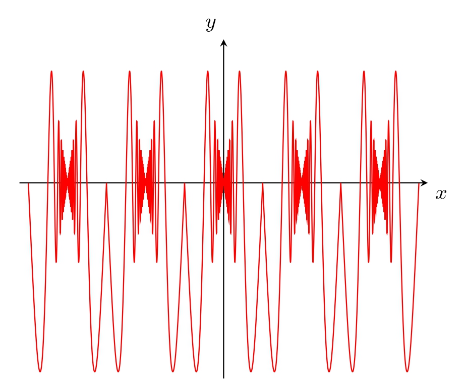
Figure 6: Example 4.9

5 Sequential necessary optimality and stationarity conditions

To embed problem (${P}$) into the model studied in Section 2, given a $\mu_{0}\in\mathbb{R}$, we consider a pair of sets in $X\times\mathbb{R}$:

$$\Omega_{1}:={\rm epi}\,f\;\;\text{and}\;\;\Omega_{2}:=\Omega\times(-\infty,\mu_{0}].$$ (30)

We are going to use the maximum product norms of the type (3) and the corresponding dual norms.

The next proposition relates the properties in Definition 4.1 with the corresponding ones in Definition 2.1.

Proposition 5.1.

Let $\mu_{0}\in\mathbb{R}$, and the sets $\Omega_{1}$ and $\Omega_{2}$ be given by (30).

1. If $\{x^{k}\}\subset\Omega$ is firmly $\inf$-stationary for (${P}$) at level $\mu_{0}$, then $\{\Omega_{1},\Omega_{2}\}$ is extremal at $\{(x^{k},f(x^{k}))\}\subset\Omega_{1}$ and $\{(x^{k},\mu_{0})\}\subset\Omega_{2}$.

2. If $\{x^{k}\}\subset\Omega$ is $\inf$-stationary for (${P}$) at level $\mu_{0}$, then $\{\Omega_{1},\Omega_{2}\}$ is stationary at $\{(x^{k},f(x^{k}))\}\subset\Omega_{1}$ and $\{(x^{k},\mu_{0})\}\subset\Omega_{2}$.

3. If $\{x^{k}\}\subset X$ is approximately $\inf$-stationary for (${P}$) at level $\mu_{0}$, then $\{\Omega_{1},\Omega_{2}\}$ is approximately stationary at $\{(x^{k},\mu_{0})\}$.

Proof.

1. Let a sequence $\{x^{k}\}\subset\Omega$ be firmly $\inf$-stationary for problem (${P}$) at level $\mu_{0}$, i.e., $f(x^{k})\to\mu_{0}$ as $k\to+\infty$, and there is a $\rho\in(0,+\infty]$ such that condition (27) is satisfied. Then

   $$\lim_{k\to+\infty}{\rm diam}\,\{(x^{k},f(x^{k})),(x^{k},\mu_{0})\}=\lim_{k\to+\infty}|f(x^{k})-\mu_{0}|=0,$$ (31)

   $$\limsup_{k\to+\infty}\Big{(}\inf_{\Omega\cap B_{\rho}(x^{k})}f-f(x^{k})\Big{)}=\limsup_{k\to+\infty}\inf_{\Omega\cap B_{\rho}(x^{k})}f-\mu_{0}=0.$$ (32)

   Let $\varepsilon>0$. By (32), there exists an integer $k>\varepsilon^{-1}$ such that $\inf_{\Omega\cap B_{\rho}(x^{k})}f-f(x^{k})>-2\varepsilon$. Choose an $\alpha\in(0,\varepsilon)$ so that

   $$\inf_{\Omega\cap B_{\rho}(x^{k})}f-f(x^{k})>-2\alpha.$$ (33)

   Set $a_{1}:=(0,-\alpha)$ and $a_{2}:=(0,\alpha)$. Thus, $\left|\kern-1.07639pt\left|\kern-1.07639pt\left|(a_{1},a_{2})\right|\kern-1.07639pt\right|\kern-1.07639pt\right|=\alpha<\varepsilon$ and, thanks to (33),

   $$(\Omega_{1}-(x^{k},f(x^{k}))-a_{1})\cap(\Omega_{2}-(x^{k},\mu_{0})-a_{2})\cap(\rho\mathbb{B}_{X\times\mathbb{R}})$$

   $$= \{(u-x^{k},\mu)\mid u\in\Omega\cap B_{\rho}(x^{k}),\;\mu\geq f(u)-f(x^{k})+\alpha,\;-\rho<\mu\leq-\alpha\}=\emptyset,$$

   i.e., $\{\Omega_{1},\Omega_{2}\}$ is extremal at sequences $\{(x^{k},f(x^{k}))\}\subset\Omega_{1}$ and $\{(x^{k},\mu_{0})\}\subset\Omega_{2}$.

2. Let a sequence $\{x^{k}\}\subset\Omega$ be $\inf$-stationary for problem (${P}$) at level $\mu_{0}$, i.e., $f(x^{k})\to\mu_{0}$ as $k\to+\infty$, and condition (28) is satisfied. Then, condition (31) holds true. Let $\varepsilon>0$. By (28), there exist an integer $k>\varepsilon^{-1}$, and a $\rho\in(0,\varepsilon)$ such that $\inf_{\Omega\cap B_{\rho}(x^{k})}f-f(x^{k})>-2\varepsilon\rho$. Choose an $\alpha\in(0,\varepsilon)$ so that

   $$\inf_{\Omega\cap B_{\rho}(x^{k})}f-f(x^{k})>-2\alpha\rho.$$ (34)

   Set $a_{1}:=(0,-\alpha\rho)$ and $a_{2}:=(0,\alpha\rho)$. Thus, $\left|\kern-1.07639pt\left|\kern-1.07639pt\left|(a_{1},a_{2})\right|\kern-1.07639pt\right|\kern-1.07639pt\right|=\alpha\rho<\varepsilon\rho$ and, thanks to (34),

   $$(\Omega_{1}-(x^{k},f(x^{k}))-a_{1})\cap(\Omega_{2}-(x^{k},\mu_{0})-a_{2})\cap(\rho\mathbb{B}_{X\times\mathbb{R}})$$

   $$= \{(u-x^{k},\mu)\mid u\in\Omega\cap B_{\rho}(x^{k}),\;\mu\geq f(u)-f(x^{k})+\alpha\rho,\;-\rho<\mu\leq-\alpha\rho\}=\emptyset,$$

   i.e., $\{\Omega_{1},\Omega_{2}\}$ is stationary at sequences $\{(x^{k},f(x^{k}))\}\subset\Omega_{1}$ and $\{(x^{k},\mu_{0})\}\subset\Omega_{2}$.

3. Let a sequence $\{x^{k}\}\subset X$ be approximately $\inf$-stationary for problem (${P}$) at level $\mu_{0}$, i.e., condition (29) is satisfied. Let $\varepsilon>0$. By (29), there exist an integer $k>\varepsilon^{-1}$, a $\rho\in(0,\varepsilon)$ and $x\in\Omega$ such that $\|x-x^{k}\|<\varepsilon$, $|f(x)-\mu_{0}|<\varepsilon$, and $\inf_{\Omega\cap B_{\rho}(x)}f-f(x)>-2\varepsilon\rho$. Then $\left|\kern-1.07639pt\left|\kern-1.07639pt\left|(x,f(x))-(x^{k},\mu_{0})\right|\kern-1.07639pt\right|\kern-1.07639pt\right|<\varepsilon$ and $\left|\kern-1.07639pt\left|\kern-1.07639pt\left|(x,\mu_{0})-(x^{k},\mu_{0})\right|\kern-1.07639pt\right|\kern-1.07639pt\right|<\varepsilon$. Choose an $\alpha\in(0,\varepsilon)$ so that

   $$\inf_{\Omega\cap B_{\rho}(x)}f-f(x)>-2\alpha\rho.$$ (35)

   Set $a_{1}:=(0,-\alpha\rho)$ and $a_{2}:=(0,\alpha\rho)$. Thus, $\left|\kern-1.07639pt\left|\kern-1.07639pt\left|(a_{1},a_{2})\right|\kern-1.07639pt\right|\kern-1.07639pt\right|=\alpha\rho<\varepsilon\rho$ and, thanks to (35),

   $$(\Omega_{1}-(x,f(x))-a_{1})\cap(\Omega_{2}-(x,\mu_{0})-a_{2})\cap(\rho\mathbb{B}_{X\times\mathbb{R}})$$

   $$= \{(u-x,\mu)\mid u\in\Omega\cap B_{\rho}(x),\;\mu\geq f(u)-f(x)+\alpha\rho,\;-\rho<\mu\leq-\alpha\rho\}=\emptyset,$$

   i.e., $\{\Omega_{1},\Omega_{2}\}$ is approximately stationary at the sequence $\{(x^{k},\mu_{0})\}$.

∎

In view of Remark 4.6 (ii), the next statement is a consequence of the sequential extremal principle in Corollary 3.4 applied to the pair of sets $\{\Omega_{1},\Omega_{2}\}$ given by (30).

Theorem 5.2 (Sequential necessary conditions).

Let $X$ be Banach, $f:X\to\mathbb{R}_{\infty}$ be lower semicontinuous, and $\Omega\subset X$ be closed. Suppose that $\{x^{k}\}\subset X$ is a minimizing sequence for problem (${P}$) at level $\mu_{0}\in\mathbb{R}$. The following assertions hold true:

1. for any $\varepsilon>0$, there exist an integer $k>\varepsilon^{-1}$, and points $(x_{1},\mu_{1})\in{\rm epi}\,f\cap B_{\varepsilon}(x^{k},\mu_{0})$, $x_{2}\in\Omega\cap B_{\varepsilon}(x^{k})$, $(x_{1}^{*},\nu_{1})\in N^{C}_{{\rm epi}\,f}(x_{1},\mu_{1})$ and $x_{2}^{*}\in N^{C}_{\Omega}(x_{2})$ such that

   $$\|x^{*}_{1}+x^{*}_{2}\|<\varepsilon\;\;\text{and}\;\;\|x^{*}_{1}\|+\|x^{*}_{2}\|+|\nu_{1}|=1.$$

2. If $X$ is Asplund, then $N^{C}$ in (i) can be replaced by $N^{F}$.

Proof.

By Remark 4.6 (ii), $\{x^{k}\}$ is firmly $\inf$-stationary for problem (${P}$) at level $\mu_{0}$. By the assumptions, the sets $\Omega_{1}$ and $\Omega_{2}$ given by (30) are closed. By Proposition 5.1 (i), $\{\Omega_{1},\Omega_{2}\}$ is extremal at $\{(x^{k},f(x^{k}))\}\subset\Omega_{1}$ and $\{(x^{k},\mu_{0})\}\subset\Omega_{2}$.

Let $\varepsilon>0$. Set $\varepsilon^{\prime}:=\frac{\varepsilon}{2+\varepsilon}$ and observe that $\varepsilon^{\prime}\in(0,1)$ and $\varepsilon^{\prime}<\varepsilon$. By Corollary 3.4 (ii) and taking into account that $f(x^{k})\to\mu_{0}$, there exist an integer $k>(\varepsilon^{\prime})^{-1}$, and points $(x_{1},\mu_{1})\in{\rm epi}\,f\cap B_{\varepsilon^{\prime}}(x^{k},f(x^{k}))$, $(x_{2},\mu_{2})\in\Omega_{2}\cap B_{\varepsilon^{\prime}}(x^{k},\mu_{0})$, $(x_{1}^{*},\nu_{1})\in N^{C}_{{\rm epi}\,f}(x_{1},\mu_{1})$, and $(x_{2}^{*},\nu_{2})\in N^{C}_{\Omega_{2}}(x_{2},\mu_{2})$ such that $|f(x^{k})-\mu_{0}|<\varepsilon-\varepsilon^{\prime}$,

$$\|x^{*}_{1}+x^{*}_{2}\|+|\nu_{1}+\nu_{2}|<\varepsilon^{\prime}\;\;\text{and}\;\;\|x^{*}_{1}\|+\|x^{*}_{2}\|+|\nu_{1}|+|\nu_{2}|=1.$$

Then $(x_{1},\mu_{1})\in{\rm epi}\,f\cap B_{\varepsilon}(x^{k},\mu_{0})$, $x_{2}\in\Omega\cap B_{\varepsilon}(x^{k})$, $x_{2}^{*}\in N^{C}_{\Omega}(x_{2})$ and

$$2(\|x^{*}_{1}\|+\|x^{*}_{2}\|+|\nu_{1}|)\geq\|x^{*}_{1}\|+\|x^{*}_{2}\|+2|\nu_{1}|=1+|\nu_{1}|-|\nu_{2}|\geq 1-|\nu_{1}+\nu_{2}|>1-\varepsilon^{\prime}>0.$$

Scaling the vectors $(x_{1}^{*},\nu_{1})\in N^{C}_{{\rm epi}\,f}(x_{1},\mu_{1})$ and $x_{2}^{*}\in N^{C}_{\Omega}(x_{2})$, one can ensure that (keeping the original notations) $\|x^{*}_{1}\|+\|x^{*}_{2}\|+|\nu_{1}|=1$ and $\|x^{*}_{1}+x^{*}_{2}\|<\frac{2\varepsilon^{\prime}}{1-\varepsilon^{\prime}}=\varepsilon$.

If $X$ is Asplund, then $N^{C}$ in the above arguments can be replaced by $N^{F}$. ∎

Corollary 5.3.

Under the assumptions of Theorem 5.2, one of the following assertions holds true:

1. there is an $M>0$ such that, for any $\varepsilon>0$, there exist an integer $k>\varepsilon^{-1}$, and points $x_{1}\in B_{\varepsilon}(x^{k})$, $x_{2}\in\Omega\cap B_{\varepsilon}(x^{k})$ such that $f(x_{1})<\inf_{\Omega}f+\varepsilon$ and

   $$0\in\partial^{C}f(x_{1})+N^{C}_{\Omega}(x_{2})\cap(M\mathbb{B}_{X^{*}})+\varepsilon\mathbb{B}_{X^{*}};$$ (36)

2. for any $\varepsilon>0$, there exist an integer $k>\varepsilon^{-1}$, and points $(x_{1},\mu_{1})\in{\rm epi}\,f\cap B_{\varepsilon}(x^{k},\mu_{0})$, $x_{2}\in\Omega\cap B_{\varepsilon}(x^{k})$, $(x_{1}^{*},\nu_{1})\in N^{C}_{{\rm epi}\,f}(x_{1},\mu_{1})$ and $x_{2}^{*}\in N^{C}_{\Omega}(x_{2})$ such that $-\varepsilon<\nu_{1}\leq 0$ and

   $$\|x^{*}_{1}+x^{*}_{2}\|<\varepsilon,\;\;\|x^{*}_{1}\|+\|x^{*}_{2}\|=1.$$

If $X$ is Asplund, then $N^{C}$ and $\partial^{C}$ in the above assertions can be replaced by $N^{F}$ and $\partial^{F}$, respectively.

Proof.

By Theorem 5.2, for any $j\in\mathbb{N}$, there exist an integer $k>j$, and points $(x_{1j},\mu_{1j})\in{\rm epi}\,f\cap B_{1/j}(x^{k},\mu_{0})$, $x_{2j}\in\Omega\cap B_{1/j}(x^{k})$, $(x_{1j}^{*},\nu_{1j})\in N^{C}_{{\rm epi}\,f}(x_{1j},\mu_{1j})$ and $x_{2j}^{*}\in N^{C}_{\Omega}(x_{2j})$ such that

$$\|x^{*}_{1j}+x^{*}_{2j}\|<1/j,\;\;\|x^{*}_{1j}\|+\|x^{*}_{2j}\|+|\nu_{1j}|=1.$$

Note that $\nu_{1j}\leq 0$ for all $j\in\mathbb{N}$. We consider two cases.
Case 1. $\limsup_{j\to+\infty}|\nu_{1j}|>\alpha>0$. Note that $\alpha<1$. Set $M:=1/\alpha$. Let $\varepsilon>0$. Choose a number $j\in\mathbb{N}$ so that $j>(\alpha\varepsilon)^{-1}$ and $|\nu_{1j}|>\alpha$. Then $\mu_{1j}=f(x_{1j})$ and $x^{*}_{1j}/|\nu_{1j}|\in\partial^{C}f(x_{1j})$. Note that $j>\varepsilon^{-1}$. Set $x_{1}:=x_{1j}$, $x_{2}:=x_{2j}$, $x_{1}^{*}:=x_{1j}^{*}/|\nu_{1j}|$, and $x_{2}^{*}:=x_{2j}^{*}/|\nu_{1j}|$. Then $x_{1}\in B_{\varepsilon}(x^{k})$, $x_{2}\in\Omega\cap B_{\varepsilon}(x^{k})$, $|f(x_{1})-\mu_{0}|<\varepsilon$, $x_{1}^{*}\in\partial^{C}f(x_{1})$, $x_{2}^{*}\in N^{C}_{\Omega}(x_{2})$, $\|x_{2}^{*}\|<1/\alpha=M$, and $\|x_{1}^{*}+x_{2}^{*}\|=\|x_{1j}^{*}+x_{2j}^{*}\|/|\nu_{1j}|<1/(\alpha j)<\varepsilon$. Hence, condition (36) is satisfied.
Case 2. $\lim_{j\to+\infty}|\nu_{1j}|=0$. Then $x_{1j}^{*}+x_{2j}^{*}\to 0$ and $1\geq\|x_{1j}^{*}\|+\|x_{2j}^{*}\|\to 1$ as $j\to+\infty$. Let $\varepsilon>0$. Choose a number $j\in\mathbb{N}$ so that $j>\varepsilon^{-1}$,

$$\gamma:=\|x_{1j}^{*}\|+\|x_{2j}^{*}\|>0,\;\;|\nu_{1j}|/\gamma<\varepsilon,\;\;\|x_{1j}^{*}+x_{2j}^{*}\|/\gamma<\varepsilon.$$

Set $x_{1}:=x_{1j}$, $\mu_{1}:=\mu_{1j}$, $x_{2}:=x_{2j}$, $x_{1}^{*}:=x_{1j}^{*}/\gamma$, $x_{2}^{*}:=x_{2j}^{*}/\gamma$, and $\nu_{1}:=\nu_{1j}/\gamma$. Then $(x_{1},\mu_{1})\in{\rm epi}\,f\cap B_{\varepsilon}(x^{k},\mu_{0})$, $x_{2}\in\Omega\cap B_{\varepsilon}(x^{k})$, $(x_{1}^{*},\nu_{1})\in N^{C}_{{\rm epi}\,f}(x_{1},\mu_{1})$, $x_{2}^{*}\in N^{C}_{\Omega}(x_{2})$, $-\varepsilon<\nu_{1}\leq 0$, $\|x_{1}^{*}\|+\|x_{2}^{*}\|=1$, and $\|x_{1}^{*}+x_{2}^{*}\|<\varepsilon$.

If $X$ is Asplund, then $N^{C}$ and $\partial^{C}$ in the above arguments can be replaced by $N^{F}$ and $\partial^{F}$, respectively. ∎

Remark 5.4.

1. The necessary conditions in Theorem 5.2 and Corollary 5.3 are applicable to any type of stationary sequences in Definition 4.5. Moreover, the generalized separation Theorem 3.2, whose Corollary 3.4 is the core tool in the proof of Theorem 5.2, allows one to derive necessary conditions for “almost minimizing” sequences.

2. Part (i) of Corollary 5.3 gives a kind of multiplier rule (in the normal form), while part (ii) corresponds to ‘singular’ behaviour of $f$ on $\Omega$ with the normal vector $(x_{1}^{*},\nu_{1})$ to the epigraph of $f$ being “almost horizontal”. If $\mu_{1}>f(x_{1})$ in part (ii), then $\nu_{1}=0$ and $x_{1}^{*}$ is normal to ${\rm dom}\,f$ at $x_{1}$.

The next qualification condition excludes the singular behavior in Corollary 5.3 (ii).

1. 1. there is an $\varepsilon>0$ such that $\|x_{1}^{*}+x_{2}^{*}\|\geq\varepsilon$ for all integers $k>\varepsilon^{-1}$, and points $(x_{1},\mu_{1})\in{\rm epi}\,f\cap B_{\varepsilon}(x^{k},\mu_{0})$, $x_{2}\in\Omega\cap B_{\varepsilon}(x^{k})$, $(x_{1}^{*},\nu_{1})\in N^{C}_{{\rm epi}\,f}(x_{1},\mu_{1})$ and $x_{2}^{*}\in N^{C}_{\Omega}(x_{2})$ such that $-\varepsilon<\nu_{1}\leq 0$ and $\|x_{1}^{*}\|+\|x_{2}^{*}\|=1$.

We denote by $(QC)_{F}$ the analogue of $(QC)_{C}$ with $N^{F}$ and $\partial^{F}$ in place of $N^{C}$ and $\partial^{C}$, respectively. Clearly, $(QC)_{C}$ $\Rightarrow\$$(QC)_{F}$.

The next statement is a direct consequence of Corollary 5.3.

Corollary 5.5.

Suppose the assumptions of Theorem 5.2 and condition $(QC)_{C}$ are satisfied. Then assertion (i) in Corollary 5.3 holds true.

If $X$ is Asplund and condition $(QC)_{F}$ is satisfied, then assertion (i) in Corollary 5.3 holds true with $N^{F}$ and $\partial^{F}$ in place of $N^{C}$ and $\partial^{C}$, respectively.

Condition $(QC)_{F}$ is ensured by the transversality of the sets ${\rm epi}\,f$ and $\Omega\times\mathbb{R}$.

Proposition 5.6.

Let $\{x^{k}\}\subset\Omega$ and $\mu_{0}\in\mathbb{R}$. If $\{{\rm epi}\,f,\Omega\times\mathbb{R}\}$ is transversal at $\{(x^{k},\mu_{0})\}$, then condition $(QC)_{F}$ holds true.

Proof.

Let $\{{\rm epi}\,f,\Omega\times\mathbb{R}\}$ be transversal at $\{(x^{k},\mu_{0})\}$. If $(x^{*},\nu)\in N^{F}_{{\rm epi}\,f}(x,\mu)$ for some $(x,\mu)\in{\rm epi}\,f$, then $\nu\leq 0$. If $(x^{*},\nu)\in N^{F}_{\Omega\times\mathbb{R}}(x,\mu)$ for some $(x,\mu)\in\Omega\times\mathbb{R}$, then $\nu=0$. By Corollary 3.10 and Remark 3.11, there is an $\varepsilon>0$ such that $\max\{\|x_{1}^{*}+x_{2}^{*}\|,|\nu_{1}|\}\geq\varepsilon$ for all integers $k>\varepsilon^{-1}$, and points $(x_{1},\mu_{1})\in{\rm epi}\,f\cap B_{\varepsilon}(x^{k},\mu_{0})$, $x_{2}\in\Omega\cap B_{\varepsilon}(x^{k})$, $(x_{1}^{*},\nu_{1})\in N^{F}_{{\rm epi}\,f}(x_{1},\mu_{1})$ and $x_{2}^{*}\in N^{F}_{\Omega}(x_{2})$ with $\|x_{1}^{*}\|+\|x_{2}^{*}\|+|\nu_{1}|=1$.

Take any integer $k>\varepsilon^{-1}$, and points $(x_{1},\mu_{1})\in{\rm epi}\,f\cap B_{\varepsilon}(x^{k},\mu_{0})$, $x_{2}\in\Omega\cap B_{\varepsilon}(x^{k})$, $(x_{1}^{*},\nu_{1})\in N^{F}_{{\rm epi}\,f}(x_{1},\mu_{1})$ and $x_{2}^{*}\in N^{F}_{\Omega}(x_{2})$ such that $-\varepsilon<\nu_{1}\leq 0$ and $\|x_{1}^{*}\|+\|x_{2}^{*}\|=1$. Set $\alpha:=1+|\nu_{1}|$, $x_{1}^{\prime*}:=x_{1}^{*}/\alpha$, $x_{2}^{\prime*}:=x_{2}^{*}/\alpha$, $\nu_{1}^{\prime}:=\nu_{1}/\alpha$. Then $(x_{1}^{\prime*},\nu_{1}^{\prime})\in N^{F}_{{\rm epi}\,f}(x_{1},\mu_{1})$, $x_{2}^{\prime*}\in N^{F}_{\Omega}(x_{2})$ and $\|x_{1}^{\prime*}\|+\|x_{2}^{\prime*}\|+|\nu_{1}^{\prime}|=1/\alpha+|\nu_{1}|/\alpha=1$. Hence, $\max\{\|x_{1}^{\prime*}+x_{2}^{\prime*}\|,|\nu_{1}^{\prime}|\}\geq\varepsilon$, and consequently, $\max\{\|x_{1}^{*}+x_{2}^{*}\|,|\nu_{1}|\}\geq\varepsilon\alpha\geq\varepsilon$. Since $|\nu_{1}|<\varepsilon$, the last inequality yields $\|x_{1}^{*}+x_{2}^{*}\|\geq\varepsilon$. Thus, condition $(QC)_{F}$ holds true. ∎

The transversality condition in Proposition 5.6 is satisfied, for instance, if $f$ is Lipschitz continuous (near a tail of the sequence $\{x^{k}\}$) or when (a tail of) the sequence $\{x^{k}\}$ lies in ${\rm int}\,\Omega$. It is not difficult to show that these conditions ensure both $(QC)_{F}$ and $(QC)_{C}$; cf. [12].

The next example illustrates Corollary 5.5.

Example 5.7 (Sequential necessary conditions).

Let $\Omega=\mathbb{R}$, $f(x)=1/x$ for all $x\neq 0$ and $f(0)=+\infty$. By Example 4.4, the sequence $x_{k}:=k$, $k=1,2,\ldots$, is minimizing for (${P}$). The function $f$ is Lipschitz continuous on $[1,+\infty)$, and consequently, conditions $(QC)_{C}$ and $(QC)_{F}$ are satisfied. By Corollary 5.5, assertion (i) in Corollary 5.3 holds true. Indeed, we obviously have $N_{\Omega}(x)=\{0\}$ for all $x\in\Omega$ and $\partial^{C}f(x)=\partial^{F}f(x)=\{-1/x^{2}\}$ (and we write simply $\partial f(x)$) for all $x\in X$. Hence, given any $\varepsilon>0$, conditions $|f(x)|<\varepsilon$ and $0\in\partial f(x)+(-\varepsilon,\varepsilon)$ are trivially satisfied when $x>0$ is large enough. The latter condition is exactly (36).

The model studied in Section 2 allows one to derive necessary optimality and stationarity conditions in more general than (${P}$) optimization problems with functional and geometric constraints, and vector or set-valued objectives.

6 Conclusions

The sequential extremality (together with sequential versions of the related concepts of stationarity, approximate stationarity and transversality) of a finite collection of sets are studied. The properties correspond to replacing a fixed point (extremal point) in the intersection of the sets by a collection of sequences of points in the individual sets with the distances between the corresponding points tending to zero. This allows one to consider collections of unbounded sets with empty intersection.

The sequential extremal principle extending the conventional one is established in terms of Fréchet and Clarke normal cones. This result can replace the conventional extremal principle when proving optimality, stationarity, transversality and regularity conditions, and calculus formulas in more general settings involving unbounded sets. In this paper, as an illustration, it is used to derive sequential necessary conditions for minimizing (and more general firmly stationary, stationary and approximately stationary) sequences in a scalar optimization problem with a geometric constraint.

Other potential applications worth being studied:

• sequential necessary optimality and stationarity conditions for optimization problems with scalar, vector and set-valued objectives and several functional and geometric constraints;

• sequential transversality and subtransversality properties of collections of sets;

• sequential metric regularity and subregularity of set-valued mappings;

• sequential error bounds of extended-real-valued functions;

• sequential qualification conditions;

• sequential extensions of limiting normal cones, subdifferentials and coderivatives, and their calculus.

Disclosure statement

No potential conflict of interest was reported by the authors.

Funding

Nguyen Duy Cuong is supported by Vietnam National Program for the Development of Mathematics 2021-2030 under grant number B2023-CTT-09.

ORCID

Nguyen Duy Cuong http://orcid.org/0000-0003-2579-3601
Alexander Y. Kruger http://orcid.org/0000-0002-7861-7380

References

[1]
Kruger AY, Mordukhovich BS. Extremal points and the Euler equation in
nonsmooth optimization problems. Dokl Akad Nauk BSSR.
1980;24(8):684–687. In Russian. Available from:
https://asterius.federation.edu.au/akruger.
[2]
Mordukhovich BS, Shao Y. Extremal characterizations of Asplund spaces. Proc
Amer Math Soc. 1996;124(1):197–205.
[3]
Mordukhovich BS. Variational analysis and generalized differentiation. I:
Basic theory. (Grundlehren der Mathematischen Wissenschaften [Fundamental
Principles of Mathematical Sciences]; Vol. 330). Berlin: Springer; 2006.
[4]
Kruger AY. Generalized differentials of nonsmooth functions and necessary
conditions for an extremum. Sibirsk Mat Zh. 1985;26(3):78–90.
(In Russian; English transl.: Siberian Math. J. 26 (1985), 370–379).
[5]
Kruger AY. On Fréchet subdifferentials. J Math Sci (NY).
2003;116(3):3325–3358.
[6]
Mordukhovich BS. Variational analysis and generalized differentiation. II:
Applications. (Grundlehren der Mathematischen Wissenschaften [Fundamental
Principles of Mathematical Sciences]; Vol. 331). Berlin: Springer; 2006.
[7]
Borwein JM, Zhu QJ. Techniques of variational analysis. New York: Springer;
2005.
[8]
Bui HT, Kruger AY. Extremality, stationarity and generalized separation of
collections of sets. J Optim Theory Appl. 2019;182(1):211–264.
[9]
Ekeland I. On the variational principle. J Math Anal Appl.
1974;47:324–353.
[10]
Fabian M. Subdifferentiability and trustworthiness in the light of a new
variational principle of Borwein and Preiss. Acta Univ Carolinae.
1989;30:51–56.
[11]
Phelps RR. Convex functions, monotone operators and differentiability. 2nd ed.
(Lecture Notes in Mathematics; Vol. 1364). Springer-Verlag, Berlin; 1993.
[12]
Cuong ND, Kruger AY. Generalized separation of collections of sets. Preprint,
arXiv:. 2024;2412.05336.
[13]
Zheng XY, Ng KF. The Fermat rule for multifunctions on Banach spaces. Math
Program. 2005;104(1):69–90.
[14]
Zheng XY, Ng KF. A unified separation theorem for closed sets in a Banach
space and optimality conditions for vector optimization. SIAM J Optim.
2011;21(3):886–911.
[15]
Cuong ND, Kruger AY, Thao NH. Extremality of families of sets. Optimization.
2024;73(12):3593–3607.
[16]
Kruger AY. About extremality of systems of sets. Dokl Nats Akad Nauk Belarusi.
1998;42(1):24–28. In Russian. Available from:
https://asterius.federation.edu.au/akruger.
[17]
Kruger AY. Strict -subdifferentials and extremality
conditions. Optimization. 2002;51(3):539–554.
[18]
Kruger AY. Weak stationarity: eliminating the gap between necessary and
sufficient conditions. Optimization. 2004;53(2):147–164.
[19]
Kruger AY. Stationarity and regularity of set systems. Pac J Optim.
2005;1(1):101–126.
[20]
Kruger AY. About regularity of collections of sets. Set-Valued Anal.
2006;14(2):187–206.
[21]
Kruger AY. About stationarity and regularity in variational analysis. Taiwanese
J Math. 2009;13(6A):1737–1785.
[22]
Bui HT, Kruger AY. About extensions of the extremal principle. Vietnam J Math.
2018;46(2):215–242.
[23]
Nguyen MT, Pham TS. Clarke’s tangent cones, subgradients, optimality
conditions, and the Lipschitzness at infinity. SIAM J Optim.
2024;34(2):1732–1754.
[24]
Kim DS, Nguyen MT, Pham TS. Subdifferentials at infinity and applications in
optimization. Math Program, Ser A. 2025;.
[25]
Clarke FH. Optimization and nonsmooth analysis. New York: John Wiley & Sons
Inc.; 1983.
[26]
Kruger AY, Thao NH. About uniform regularity of collections of sets. Serdica
Math J. 2013;39(3-4):287–312.