AI-Powered Noisy Quantum Emulation: Generalized Gate-Based Protocols for Hardware-Agnostic Simulation

Abstract

Quantum computer emulators model the behavior and error rates of specific quantum processors. Without accurate noise models in these emulators, it is challenging for users to optimize and debug executable quantum programs prior to running them on the quantum device, as device-specific noise is not properly accounted for. To overcome this challenge, we introduce a general protocol to approximate device-specific emulators without requiring pulse-level control. By applying machine learning to data obtained from gate set tomography, we construct a device-specific emulator by predicting the noise model input parameters that best match the target device. We demonstrate the effectiveness of our protocol’s emulator in estimating the unitary coupled cluster energy of the H₂ molecule and compare the results with those from actual quantum hardware. Remarkably, our noise model captures device noise with high accuracy, achieving a mean absolute difference of just 0.3% in expectation value relative to the state-vector simulation.

I Introduction

In the current noisy intermediate-scale quantum [1] (NISQ) computing era, access to quantum computers are predominantly cloud-based [2, 3, 4, 5, 6, 7]. Despite the host of available NISQ computers from different service providers, their accessibility is often limited or costly; users can be subjected to long queuing times or have to pay for circuit executions. Costs will increase when compute-intensive problems require many iterations, especially when using quantum algorithms that are variational in nature [8, 9, 10]. As a result, despite variational quantum algorithms being the most prevalent type of quantum algorithm for NISQ computers [10, 11, 12], with the exception of simple toy problems, it is unfeasible for most users to perform the definitive routine of quantum circuit parameter optimization directly on NISQ computers. Instead, parameter optimization is often done via classical simulations, and the optimized variational quantum circuit is then run on the NISQ device for validation or comparison [13, 14].

To maximize the efficiency of the validation run on NISQ computers, it is crucial to have classical simulators that can faithfully replicate the behavior of individual NISQ devices through device-specific emulators. Users can construct an emulator for their chosen quantum computer, but not all input parameters required for a comprehensive noise model are regularly updated or readily available from the hardware provider. These parameters are derived from calibration protocols that require access to pulse-level control. In the absence of device-specific emulators, users typically rely on noiseless state-vector simulations of their quantum algorithms, the results of which would substantially deviate from those obtained on currently available NISQ devices. The lack of such device-specific emulators makes job submissions to NISQ devices costly and time-consuming, with limited conclusions drawn from the results.

Without the latest calibration data, general users can only perform gate-based characterization protocols such as randomized benchmarking [15, 16] and gate set tomography (GST) [17, 18, 19] to partially profile the noise of the NISQ device. All other device characteristics needed for a more complete and up-to-date noise model such as the qubit relaxation time from the $\ket{1}$ to $\ket{0}$ state (T1 time), the time that qubits preserve coherence (T2 time), as well as calibrated native gate times are excluded from the noise profile. Moreover, it is impractical for a resource-limited user to perform certain gate-based protocols such as process tomography on every native gate.

Recognizing the need for realistic emulators of hardware, several approaches have been proposed to model device noise. Prior work has explored parameter optimization of thermal relaxation and depolarizing noise [20, 21]. Other methods apply noise through perturbations of the Hamiltonian for single-qubit gates, Gaussian phase noise for two-qubit gates, and Gaussian coherent noise to account for control errors [22]. These approaches use an underlying physical model of the device as a starting point, such that the accuracy of the noise model depends on the physical model’s fidelity and the accessibility of precise device characterization data.

In this work, we propose a general GST-based protocol that leverages supervised machine learning to construct heuristic device noise models agnostic to device physics. The goal of our protocol is to closely approximate noise profiles of specific NISQ devices even when device-specific noise characterizations are unavailable. By applying it with a minimal composite noise model for two selected qubits of the IQM Garnet quantum processor accessed through Amazon Braket [23, 24], we demonstrate how general users can adapt our protocol to construct emulators for the NISQ device of their choice. As we will discuss in detail in Sec. II, our protocol utilizes neural networks trained on GST data simulated over a range of noise parameter values to predict the noise parameter values that best fit GST data obtained from the target NISQ device. In Sec. III, we evaluate the performance of our protocol’s emulator by benchmarking its results for a quantum chemistry task against results obtained from IQM Garnet. Our benchmark shows that not only does device noise leave footprints in GST data that can be detected and learned by neural networks, more remarkably, our emulator constructed with a minimal heuristic noise model comprising depolarizing, amplitude damping, dephasing, and readout noise channels is capable of achieving simulation results that have appreciably small deviation from the actual noisy device. To conclude, we discuss in Sec. IV the impact of our work, its wide applicability and utility, as well as follow-up work and future directions.

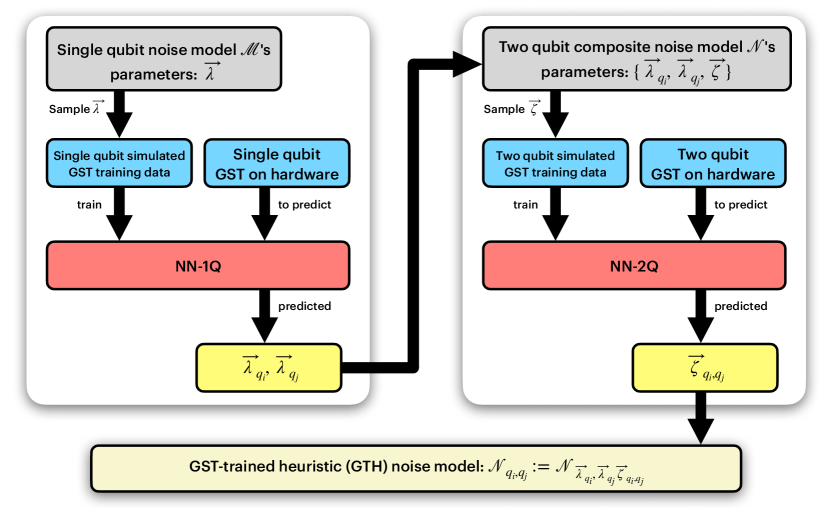
Figure 1: Schematic of the proposed AI-powered, generalized gate-based protocol for processing simulated and hardware GST data. A neural network for single-qubit noise (NN-1Q) predict noise parameters $\vec{\lambda}_{q_{i}},\vec{\lambda}_{q_{j}}$, while a neural network for two-qubits (NN-2Q) predicts $\vec{\zeta}_{q_{i},q_{j}}$ for the target qubits $q_{i}$ and $q_{j}$. These predictions are used to construct the GST-trained heuristic (GTH) noise model $\mathcal{N}_{q_{i},q_{j}}$.

II Methods

Our AI-powered, generalized gate-based protocol comprises three key components:

1. a sufficiently comprehensive noise model with a set of input noise parameters capable of emulating quantum hardware noise,

2. a set of gate-based circuits to execute on quantum hardware that serve to collect characterization data,

3. a machine learning framework to predict the noise parameters corresponding to the device based on its characterization data.

In this work, we concretize this generalized protocol by making a specific choice for each key component to construct the GST-trained heuristic (GTH) noise model. A schematic of the protocol is summarized in Fig. 1, and detailed in the following subsections.

II.1 Noise models

The first component of our protocol is a comprehensive noise model capable of emulating hardware noise. While our protocol can be adapted to different noise models, we focus on the worst-case scenario in which general users do not have access to any device characterization data. To this end, we propose a heuristic noise model where each one-qubit gate on qubit $q_{i}$ is subject to a one-qubit noise model $\mathcal{M}_{\vec{\lambda}_{q_{i}}}$, with noise parameters $\vec{\lambda}_{q_{i}}$ specific to qubit $q_{i}$. Subsequently, each two-qubit gate on qubits $q_{i}$ and $q_{j}$ is subject to a two-qubit composite noise model, $\mathcal{N}(\vec{\lambda}_{q_{i}},\vec{\lambda}_{q_{j}},\vec{\zeta}_{q_{i},q_{j}})$, comprising the respective one-qubit noise models $\mathcal{M}_{\vec{\lambda}_{q_{i}}}$ and $\mathcal{M}_{\vec{\lambda}_{q_{j}}}$, as well as additional two-qubit noise channels collectively parameterized by parameters $\vec{\zeta}_{q_{i},q_{j}}$. We chose $\mathcal{M}$ to be a composition of the depolarizing noise, amplitude damping, dephasing, and readout noise channels, collectively parameterized by $\vec{\lambda}:=(\lambda_{d},\lambda_{a},\lambda_{f},\lambda_{r})$, while we chose $\mathcal{N}$ to have an additional two-qubit depolarizing noise channel parameterized by a single parameter, $\vec{\zeta}:=\zeta$.

We define the single-qubit noise model for qubit $q_{i}$ as,

$$\mathcal{M}_{\vec{\lambda}_{q_{i}}}:=\mathcal{E}^{(n=1)}_{\lambda_{d}}(\rho)\circ\mathcal{E}_{\lambda_{a}}(\rho)\circ\mathcal{E}_{\lambda_{f}}(\rho)\circ\mathcal{E}_{\lambda_{r}}(\rho),$$ (1)

where $\mathcal{E}^{(n=1)}_{\lambda_{d}}(\rho)$ is the single-qubit depolarizing channel, $\mathcal{E}_{\lambda_{a}}(\rho)$ is the amplitude damping channel, $\mathcal{E}_{\lambda_{f}}(\rho)$ is the dephasing channel, and $\mathcal{E}_{\lambda_{r}}(\rho)$ is the readout channel.

We define the two-qubit composite noise on qubits $q_{i}$ and $q_{j}$ as,

$$\mathcal{N}_{q_{i},q_{j}} :=\mathcal{N}_{\vec{\lambda}_{q_{i}},\vec{\lambda}_{q_{j}},\vec{\zeta}}$$ (2)

$$=\mathcal{M}_{\vec{\lambda_{q_{i}}}}\circ\mathcal{M}_{\vec{\lambda_{q_{j}}}}\circ\mathcal{E}^{(n=2)}_{\lambda_{d}}(\rho),$$

where $\mathcal{E}^{(n=2)}_{\lambda_{d}}(\rho)$ is the two-qubit depolarizing channel.

Depolarizing noise transforms a $n$-qubit quantum state $\rho$ into a completely mixed state, which can be interpreted as a uniform distribution over all $2^{n}$ computational basis states. The parameter $\lambda_{d}$ indicates the probability in which the output state becomes a completely mixed state [25]. Its $n$-qubit representation is given by

$$\mathcal{E}^{(n)}_{\lambda_{d}}(\rho)=(1-\lambda_{d})\rho+\frac{\lambda_{d}I}{2^{n}},$$ (3)

where $2^{n}$ is the dimension of the quantum system and $I/2^{n}$ is the maximally mixed state.

Amplitude damping noise stems from the decay of a quantum state $\rho$ from an excited state to the ground state. The parameter $\lambda_{a}$ is associated with the probability that a state $\ket{\psi}$ decays to the state $\ket{0}$. Higher $\lambda_{a}$ values correspond to shorter times for this decay. The amplitude damping noise is usually written as a quantum channel

$$\mathcal{E}_{\lambda_{a}}(\rho)=K_{1}\rho K_{1}^{\dagger}+K_{2}\rho K_{2}^{\dagger},$$ (4)

where

$$K_{1}=\begin{pmatrix}1&0\\ 0&\sqrt{1-\lambda_{a}}\end{pmatrix}\quad\text{and}\quad K_{2}=\begin{pmatrix}0&\sqrt{\lambda_{a}}\\ 0&0\end{pmatrix},$$ (5)

are the Kraus operators [26]. In hardware calibration, amplitude damping is closely associated with the T1 time.

Dephasing noise results from the decoherence of a quantum state, thus reducing the relative phases between the quantum states over time. Similar to amplitude damping described earlier, increasing probability parameter $\lambda_{f}$ is akin to shortening the time for decoherence to occur. The dephasing noise is written as a quantum channel similar to that for amplitude damping

$$\mathcal{E}_{\lambda_{f}}(\rho)=K_{1}\rho K_{1}^{\dagger}+K_{2}\rho K_{2}^{\dagger},$$ (6)

where

$$K_{1}=\begin{pmatrix}1&0\\ 0&\sqrt{1-\lambda_{f}}\end{pmatrix}\quad\text{and}\quad K_{2}=\begin{pmatrix}0&0\\ 0&\sqrt{\lambda_{f}}\end{pmatrix},$$ (7)

are the associated Kraus operators. Dephasing noise is commonly associated with the T2 time.

The last type of noise that we considered is the readout noise. It represents errors that commonly occur during the measurements of quantum states during quantum computation. Noisy measurement outcomes can simulated by applying a row-stochastic transition matrix $P$ containing conditional probabilities to the original measurement outcomes. The matrix $P$ is given as

$$P=\begin{pmatrix}p(0|0)&p(1|0)\\ p(0|1)&p(1|1)\end{pmatrix},$$ (8)

where the elements $p(y|x)$ represent the probability of the original measurement outcome $x$ being erroneously transformed to outcome $y$. For simplicity, we let the elements $p(0|0)=p(1|1)=1-\lambda_{r}$ and $p(1|0)=p(0|1)=\lambda_{r}$. The reset error channel is essentially a bit flip quantum channel with error-free measurement and can be represented with the following quantum channel

$$\mathcal{E}_{\lambda_{f}}(\rho)=K_{1}\rho K_{1}^{\dagger}+K_{2}\rho K_{2}^{\dagger},$$ (9)

where

$$K_{1}=\begin{pmatrix}\sqrt{1-\lambda_{r}}&0\\ 0&\sqrt{1-\lambda_{r}}\end{pmatrix}\quad\text{and}\quad K_{2}=\begin{pmatrix}0&\sqrt{\lambda_{r}}\\ \sqrt{\lambda_{r}}&0\end{pmatrix},$$ (10)

are the associated Kraus operators.

We use the quantum computing software Qibo [27] as a platform to execute quantum circuits. A key feature we exploit is the stacking of multiple noise models – single-qubit and two-qubit noise models – into a singular composite noise model for subsequent application.

II.2 Gate set tomography

The second component of our protocol is a set of gate-based circuits that, when executed on quantum hardware, acquire characterization data which contain footprints of the device noise. Gate set tomography (GST) [17, 18, 19] is a technique used to characterize gates in the presence of state preparation and measurement errors. We hypothesize that applying GST on a pre-selected set of native gates would provide the required characterization data.

To carry out GST, one needs to first prepares the states $\rho_{k}\in\{\ket{0}\bra{0},\ket{1}\bra{1},\ket{+}\bra{+},\ket{y+}\bra{y+}\}^{\otimes n}$, where $n$ is the number of qubits in the system. Subsequently, an $n$-qubit gate may or may not be applied after the prepared state. Expectation values of the Pauli operators are then computed, $M_{j}=\{\langle I\rangle,\langle X\rangle,\langle Y\rangle,\langle Z\rangle\}^{\otimes n}$.

In the case where no gate is applied after the prepared state, the resulting matrix $g$ has the following elements

$$g_{jk}=\text{Tr}(M_{j}\rho_{k}).$$ (11)

The matrix $g$ may also be regarded as a calibration matrix.

When a gate $U$ is applied after the prepared state, the resulting matrix $\mathcal{U}$ contains the following elements

$$\mathcal{U}_{jk}=\text{Tr}(M_{j}U\rho_{k}).$$ (12)

For single-qubit GST ($n=1$), the resultant matrices $g$ and $\mathcal{U}$ are size 4 $\times$ 4. For two-qubit GST ($n=2$), the resultant matrices $g$ and $\mathcal{U}$ are size 16 $\times$ 16.

II.3 Gate set tomography on IQM

IQM Garnet uses the Phase Rx gate and CZ gate as its native gates. The Phase Rx gate, hereafter referred to as the PRx gate, can be decomposed into three rotational gates, $\text{PRX}(\theta,\phi)=\text{Rz}(\phi)\text{Rx}(\theta)\text{Rz}(-\phi)$. Together with the CZ gate, they form a universal gate set.

To carry out GST on the IQM Garnet device, we used a modified version of GST code to only use PRx gates for state preparations and measurements in various bases. This modification specifically allowed GST to be executed with Amazon Braket’s verbatim compilation function, bypassing the need for on-device transpilation/compilation to native gates before execution. This enabled us to have full control of target qubits for single-qubit GST as well as control and target qubits for two-qubit GST.

While searching for a suitable gate set for GST, we observed that different types of noise on different gates impact the $g$ and $\mathcal{U}$ matrices with some more similar than others. Amplitude damping noise causes all elements of $g$ and $\mathcal{U}$ to tend towards 1. Dephasing and depolarizing noise may have similar effects on $g$ and $\mathcal{U}$, depending on the choice of gate. Readout noise at a certain parameter resembles maximum depolarizing or dephasing noise as well. We provide a heuristic elaboration in Fig. 5 in Appendix B. The single-qubit PRx gates that form our gate set in Table 1.

Index	1	2	3	4	5	6	7	8	9	10	11	12	13	14	15
$\theta$	$\pi$	$\frac{\pi}{2}$	$\frac{\pi}{2}$	$\frac{\pi}{3}$	$\frac{\pi}{3}$	$\frac{\pi}{3}$	$\frac{\pi}{4}$	$\frac{\pi}{4}$	0	$\pi$	$-\frac{\pi}{2}$	$\frac{\pi}{4}$	$\frac{\pi}{7}$	$\frac{\pi}{7}$	$\frac{\pi}{7}$
$\phi$	0	$-\frac{\pi}{2}$	$\frac{\pi}{2}$	$\frac{\pi}{3}$	$\frac{\pi}{4}$	$\frac{\pi}{7}$	$\frac{\pi}{3}$	$\frac{\pi}{4}$	0	0	0	$\frac{\pi}{7}$	$\frac{\pi}{3}$	$\frac{\pi}{4}$	$\frac{\pi}{7}$

Table 1: List of PRx gates’ angles for 1 qubit gate set.

The two-qubit gate set only consists of the CZ gate as it is the only native two-qubit gate of IQM Garnet.

II.4 Recipe for constructing $\mathcal{N}_{q_{i},q_{j}}$

We outline these steps in accordance with Fig. 1 to obtain the GTH noise model for qubits $q_{i}$ and $q_{j}$.

1. Define $\vec{\lambda}:=(\lambda_{d},\lambda_{a},\lambda_{f},\lambda_{r})$, representing single-qubit depolarizing noise, amplitude damping noise, dephasing noise, and readout noise parameters, respectively.

2. Define a discrete range for $\vec{\lambda}$.

3. For each value in the range for $\vec{\lambda}$, use single-qubit noise model $\mathcal{M}_{\vec{\lambda}}$ (Eq. 1) to generate single-qubit simulated GST data. The full dataset is then used to train NN-1Q.

4. Perform single-qubit GST for qubit $q_{i}$ on hardware, input the results into the trained NN-1Q to obtain predicted noise $\vec{\lambda}_{q_{i}}$.

5. Repeat Step 4 on qubit $q_{j}$ (which is coupled to $q_{i}$) to get $\vec{\lambda}_{q_{j}}$.

6. Construct two-qubit composite noise model $\mathcal{N}_{\vec{\lambda_{q_{i}}},\vec{\lambda_{q_{j}}},\vec{\zeta}}$ (Eq. 2) where $\vec{\zeta}$ represents the two-qubit depolarizing noise.

7. Define a discrete range for $\vec{\zeta}$.

8. For each value in the range for $\vec{\zeta}$, use $\mathcal{N}_{\vec{\lambda}_{q_{i}},\vec{\lambda}_{q_{j}},\vec{\zeta}}$ to generate two-qubit simulated GST data. The full dataset is used to train NN-2Q.

9. Perform two qubit GST for qubit $q_{i}$ and $q_{j}$ on hardware, input the results into the trained NN-2Q to obtain the predicted two-qubit depolarizing noise $\vec{\zeta}_{q_{i},q_{j}}$.

10. Finally, form the GTH noise model $\mathcal{N}_{q_{i},q_{j}}:=\mathcal{N}_{\vec{\lambda}_{q_{i}},\vec{\lambda}_{q_{j}},\vec{\zeta}_{q_{i},q_{j}}}$.

We provide a more detailed explanation of the training procedure, including the choice of step sizes for $\vec{\lambda}$ and $\vec{\zeta}$, in Appendix C.

II.5 Training and evaluating neural networks for prediction

The third and final component of our protocol is a machine learning framework that can be used to predict noise parameters from GST data. For simplicity and ease of implementation, we choose two feed-forward neural networks: one to be trained on single-qubit GST data (NN-1Q) and the other to be trained on two-qubit GST data (NN-2Q). The details of the architecture of NN-1Q and NN-2Q can be found in Table 2. In addition, all data used to train NN-1Q as well as the generated data for NN-2Q, the weights of NN-1Q and NN-2Q, and the standard scalers applied to both neural networks are available at Ref. [28].

The evaluation process occurs in two stages. The first stage happens in real-time during the training of the neural network. Using a validation split parameter that determines the proportion of samples allocated to compute the validation loss function, we monitor the validation loss alongside the training loss. This feedback provides real-time analysis of overfitting (when validation loss increases while training loss decreases) or underfitting (when both validation loss and training loss remain high) of the model.

The second stage takes place after training is complete. Here, the performance of a neural network is evaluated by comparing the neural network’s predictions against ground truth values. This is done by performing GST again using predicted values of $\vec{\lambda}_{\text{true}}$ or $\vec{\zeta}_{\text{true}}$ in two settings: (a) using predetermined values of $\vec{\lambda}_{\text{true}}$ or $\vec{\zeta}_{\text{true}}$ as those used during training and (b) using predefined values of $\vec{\lambda}_{\text{true}}$ and $\vec{\zeta}_{\text{true}}$ with finer granularity than those used in training. In both cases, the newly generated GST data is fed into the neural network and the proximity of the predicted values ($\vec{\lambda}_{\text{predicted}}$ to $\vec{\lambda}_{\text{true}}$ and $\vec{\zeta}_{\text{predicted}}$ to $\vec{\zeta}_{\text{true}}$) is analyzed. The mean squared error (MSE) quantifies the distance between ground truth and predicted values. In addition, a “predicted vs true” plot provides visual confirmation.

Parameters	NN-1Q	NN-2Q
No. of intermediate layers (excluding output)	2	2
No. of nodes in intermediate layer	128	64
No. of nodes in output layer	4	1
Activation function for intermediate layers	ReLU	ReLU
Activation function for output layer	Custom sigmoid ($\alpha=8$)	Custom sigmoid ($\alpha=8$)
Optimizer	Adam	Adam
Learning rate	$10^{-4}$	$10^{-4}$
Loss function	Mean squared error	Mean squared error
L2 regularization	$5\times 10^{-5}$	$5\times 10^{-6}$
Dropout	$5\times 10^{-5}$	$5\times 10^{-6}$
Batch size	64	32
Validation split	0.2	0.2
Recommended no. of training episodes	100	1,000

Table 2: Parameters for NN-1Q and NN-2Q.

III Results

In this section, we first present the performance of NN-1Q and NN-2Q before looking at how $\mathcal{N}_{q_{i},q_{j}}$ is benchmarked against hardware results with a quantum chemistry example.

III.1 Performance of NN-1Q and NN-2Q

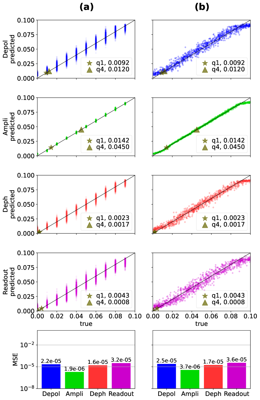
Figure 2: Evaluation of NN-1Q using (a) unseen data with predetermined ground truths values as those used during training and (b) predefined ground truths with finer granularity than those used in training. The predicted values from the IQM GST data are plotted on the $y=x$ line for visual reference. The bottom bar charts display the mean squared error (MSE) of the both evaluation settings.

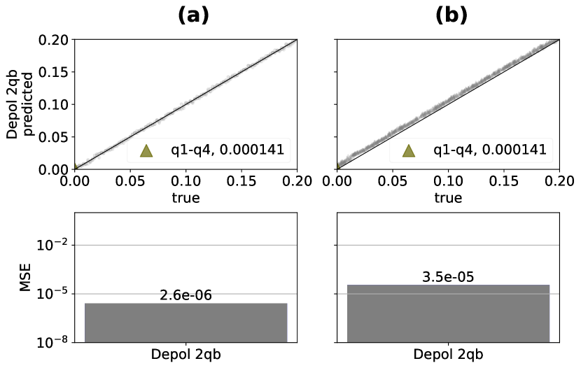
Figure 3: Evaluation of NN-2Q using (a) unseen data with predetermined ground truths values as those used during training and (b) predefined ground truths with finer granularity than those used in training. The predicted values from the IQM GST data are plotted on the $y=x$ line for visual reference but are close to zero as seen in the legends. The bottom bar charts display the mean squared error (MSE) of the both evaluation settings.

Single-qubit	$q_{1}$	$q_{4}$
$\lambda_{d}$	0.00924	0.01203
$\lambda_{a}$	0.01415	0.04505
$\lambda_{f}$	0.00228	0.00170
$\lambda_{r}$	0.00434	0.00081
Two qubit	$q_{1}$-$q_{4}$
$\zeta$	0.00014

Table 3: Predictions for qubit $q_{1}$ and qubit $q_{4}$ individually by NN-1Q and coupled qubits $q_{1}$ and $q_{4}$ by NN-2Q to 5 decimal places.

Following the protocol in Fig. 1, we performed single-qubit GST on IQM Garnet with the 15 gates listed in Table 1 on qubits $q_{1}$ and $q_{4}$ individually followed by two qubits GST, also on qubits $q_{1}$ and $q_{4}$. The calibration data for the days we performed GST was concurrently obtained and stored.

The single-qubit GST was performed with 10,000 shots while the two-qubit GST was performed with 1,000 shots. A larger shot count was necessary to reduce statistical fluctuations in the GST data, which could otherwise provide misleading higher error-ridden input data into neural network, affecting the predictions. Despite this, we found that using 1,000 shots for two-qubit GST was sufficient to predict the two-qubit depolarizing noise. Due to availability constraints, the single-qubit GST and two-qubit GST were performed on separate days.

We plot the evaluation of NN-1Q in Fig. 2 and NN-2Q in Fig. 3, illustrating the ability of NN-1Q and NN-2Q in the two types of evaluation described in Section II.5. In the “predicted versus true” plots for NN-1Q, we notice that the network’s predictions are scattered along the diagonal. This can be attributed to the impact of the finite shots used (10,000 shots) to generate the GST training data.

The prediction accuracy is quantified using the MSE, with the corresponding plots shown in the bar charts. The largest mean squared error is in the order $O(10^{-5})$, which is sufficiently small to provide a reasonable level of confidence.

Visually, we note that NN-2Q performs considerably better than the four single-qubit noise models as the predicted values have less scattering along the diagonal. It is quantitatively confirmed by a low mean squared error in the order of $O(10^{-6})$. This is solely due to NN-2Q being used to predict only one type of noise–the two qubit depolarizing noise model.

A summary of the predictions for $\vec{\lambda}_{q_{1}}$, $\vec{\lambda}_{q_{1}}$, and $\vec{\zeta}_{q_{1},q_{4}}$ is listed in Table. 3. These predictions for the noise models are used as inputs for in the composite noise model $\mathcal{N}_{q_{i},q_{j}}$.

(a)

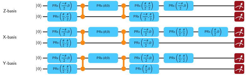
(b)

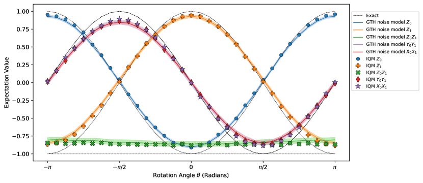
Figure 4: (a) Transpiled UCC circuits to IQM Garnet native gates for measurement in the Z, Y, and X bases. Adjusting the parameter $\theta$ from $-\pi$ to $\pi$ and executing them on IQM Garnet as well as with our noise model, we obtain the corresponding expectation values in (b). The mean absolute difference between composite noise model values and device values is $0.02168$. Note that IQM $Y_{0}Y_{1}$ and IQM $X_{0}X_{1}$ are almost identical, resulting in a large degree of overlap among the scatter points.

III.2 Application of the GTH noise model $\mathcal{N}_{q_{i},q_{j}}$: Quantum Chemistry

III.2.1 Unitary Coupled Cluster energy of the H₂ molecule

We present here a test of $\mathcal{N}_{q_{i},q_{j}}$ on an example quantum chemistry calculation, namely the unitary coupled cluster (UCC) energy of the H₂ molecule with atomic separation of 0.70Åusing the STO-6G basis set, as demonstrated by O’Malley et al. [29], we provide a detailed description of the UCC method elsewhere in Appendix A, and shall only provide the important experimental details here. The second quantized electronic Hamiltonian for the above system is transformed to the following qubit Hamiltonian after Bravyi-Kitaev [30] mapping:

$$\begin{split}\hat{H}=&-0.4584\hat{I}+0.3593\hat{Z}_{0}-0.4826\hat{Z}_{1}+0.5818\hat{Z}_{0}\hat{Z}_{1}\\ &+0.0896\hat{X}_{0}\hat{X}_{1}+0.0896\hat{Y}_{0}\hat{Y}_{1}.\end{split}$$ (13)

The ground state for the above Hamiltonian as predicted by UCC theory is

$$|\psi(\theta)\rangle=e^{-i\theta\hat{X}_{0}\hat{Y}_{1}}|\phi\rangle.$$ (14)

The state $|\phi\rangle$ is a reference state for the electrons in the molecular system. We adopt the Hartree-Fock state as $|\phi\rangle$, which is encoded big-endian here as $|10\rangle$; the first orbital is occupied and second orbital is vacant, or virtual. Using a parameterized ansatz $|\psi(\theta)\rangle=U(\theta)|\phi\rangle$ with parameter vector $\theta$ on the quantum circuit used by O’Malley et al. [29] the corresponding circuits in the basis to be measured (Z, X, or Y), transpiled to IQM Garnet’s native gates, is given in Fig. 4(a).

	Expectation value
State-vector	$-1.1473029$
IQM Garnet	$-0.9965888$
$\mathcal{N}_{q1,q4}$	$-0.9935546$

Table 4: $\mathcal{N}_{q1,q4}$ was benchmarked against IQM Garnet using the same circuits in Fig. 4(a) with the optimal parameter $\theta^{*}=0.2097$, showing similar performance as the IQM Garnet device with only a 0.3% deviation in expectation value relative to the state-vector simulation result.

Adopting a variational approach, the optimal parameter for $\theta$ that minimizes the UCC energy for H₂ was found to be $\theta^{*}=0.2097$. Substituting $\theta^{*}$ into the three circuits given in Fig. 4(a), we then ran these circuits using IQM Garnet with 10,000 shots and computed the expectation value. These exact circuits were then subjected to the noise model $\mathcal{N}_{q_{1},q_{4}}$ $\mathcal{N}\left(\vec{\lambda}_{q_{1}},\vec{\lambda}_{q_{4}},\vec{\zeta}_{q_{1},q_{4}}\right)$ and simulated classically. The results are given in Table 4.

For completeness, we ran all three circuits in Fig. 4(a) with various values for $\theta$, sweeping through $-\pi$ to $\pi$ in 33 equal steps on both IQM Garnet and with the composite noise model. We disclose here that the sweep on IQM Garnet was conducted on a separate day from the GST run due to availability constraints. Nonetheless, the composite noise model’s expectation values were compared side by side with the IQM Garnet’s expectation values in Fig. 4(b). The standard deviation for each term in the Hamiltonian is given in shaded regions. Our composite noise model is seen to emulate the IQM Garnet device very well, with a mean absolute difference of 0.02168 for the expectation value of all Pauli terms in the Hamiltonian. These encouraging results provide confidence in our composite noise model in emulating device noise, and in the GST-based machine-learning protocol used to construct it.

IV Conclusion

In this work, we constructed the GTH noise model and demonstrated its potential to accurately capture the noise on the IQM Garnet device. Our emulation of the UCC circuits for H₂ with the GTH noise model gave results with a mean absolute difference of 0.02168 from the actual hardware run, which translates to a mere 0.3% deviation in expectation value relative to the state-vector simulation result. Through achieving high-fidelity emulation of an actual quantum processor, we use the GTH noise model as a specific realization to demonstrate how general users can apply our proposed AI-powered, generalized gate-based protocol to construct a heuristic but yet effective noise model for any quantum computer of their choice.

The effectiveness of the GTH noise model shows that not only does the data obtained from GST leave substantial noise footprints of the hardware, we demonstrate how general users can exploit machine learning to turn the data used for characterizing the performance of quantum hardware to build a noise model that emulates the hardware itself. Additionally, our work shows that to closely approximate actual hardware noise, input from an underlying physical model of the device is not required and it is in fact possible to do so with heuristic noise models that are sufficiently complex. Unlike such physics-based noise models, the noise parameters of our GTH noise model are essentially fitting parameters and do not necessarily correspond to any physical characteristics of the hardware. The success of this preliminary work opens the door to achieving accurate device-noise modeling beyond physics-based approaches that may be just as or even more faithful in reproducing hardware results. Substantial improvements can be made by utilizing other candidate heuristic noise models, further optimizing the neural network design, as well as designing other gate-based device characterization circuits beyond GST.

Most importantly, our work lays the foundation for general users to gain access to accurate quantum device emulation. The protocol can be extended in a straightforward manner from a two-qubit to $n$-qubit case following the qubit connectivity of the quantum device. While it is possible to emulate the noise characteristics for a larger portion of the NISQ device, we recognize that the GST experiments required in our current protocol will nonetheless incur substantial costs to general users. Future work will explore improvements to reduce such costs, potentially through incorporating less costly experiments such as randomized benchmarking. This will enable general users to build NISQ device emulators with more qubits, allowing for simulations of larger and more complex quantum algorithms that can be meaningfully compared to hardware results.

Appendix A Unitary Coupled Cluster

For a molecular system of clamped nuclei (Born-Oppenheimer approximation), the electronic Hamiltonian in second quantization using creation and annihilation operators $\hat{a}^{\dagger}$ and $\hat{a}$ is written as

$$\hat{H}_{\mathrm{elec}}=\sum_{pq}h_{pq}\hat{a}^{\dagger}_{p}\hat{a}_{q}+\frac{1}{2}\sum_{pqrs}(pr|qs)\hat{a}^{\dagger}_{p}\hat{a}^{\dagger}_{q}\hat{a}_{s}\hat{a}_{r},$$ (15)

where $h_{pq}$ and $(pr|qs)$ are one- and two-electron integrals obtained from PySCF, $p,q,r,s$ are general orbital indices.

The Bravyi-Kitaev transformation of  15 yields the BK-transformed Hamiltonian which is in the following form,

$$\hat{H}_{\mathrm{BK}}=g_{0}\hat{I}+g_{1}\hat{Z}_{0}+g_{2}\hat{Z}_{1}+g_{3}\hat{Z}_{0}\hat{Z}_{1}+g_{4}\hat{X}_{0}\hat{X}_{1}+g_{5}\hat{Y}_{0}\hat{Y}_{1}.$$ (16)

The electronic state of this molecular system is represented using the Unitary Coupled Cluster (UCC) ansatz, a variant of the gold-standard Coupled Cluster theory in quantum chemistry. Cluster generators $\hat{T}_{n}(\theta)$ with excitation parameter $\theta$ effect n-tuple excitation of electrons from occupied orbitals $i,j,...$ to unoccupied (virtual) orbitals $a,b...$, and for singles and doubles excitations they are

$$\hat{T}_{1}(\theta_{ia}) =\sum_{ia}\theta_{ia}\hat{a}^{\dagger}_{a}\hat{a}_{i}$$ (17)

$$\hat{T}_{2}(\theta_{iajb}) =\frac{1}{4}\sum_{iajb}\theta_{iajb}\hat{a}^{\dagger}_{a}\hat{a}_{i}\hat{a}^{\dagger}_{b}\hat{a}_{j}.$$ (18)

A cluster operator $\hat{T}$ is generally

$$\hat{T}(\theta)=\hat{T}_{1}(\theta_{ia})+\hat{T}_{2}(\theta_{iajb})+\dots+\hat{T}_{m}(\theta_{(m)}),$$ (19)

where $m$ is the highest level of excitations and $(m)$ indicates the excitations for cluster generator $\hat{T}_{m}$, e.g. for singles, $m=1$, $(m)\rightarrow ia$.

Starting from a mean-field starting state, namely the Hartree-Fock state $|\phi\rangle$ obtained from a classical computation, the UCC ansatz is implemented as

$$|\psi(\theta)\rangle =U(\theta)|\phi\rangle$$ (20)

$$=e^{(\hat{T}(\theta)-\hat{T}^{\dagger}(\theta))}|\phi\rangle.$$ (21)

The electronic energy is variationally minimized to obtain the UCC energy,

$$E_{0}=\min_{\theta}\frac{\langle\psi(\theta)|\hat{H}_{\mathrm{BK}}|\psi(\theta)\rangle}{\langle\psi(\theta)|\psi(\theta)\rangle}.$$ (22)

Appendix B Gate set tomography

(a)

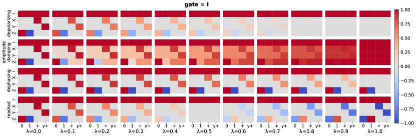
(b)

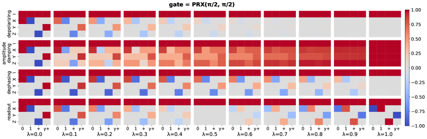
Figure 5: To illustrate the effects of different noise models on different single-qubit gates, a heatmap containing the 4 by 4 matrices for the (a) identity gate and (b) $\text{PRx}(\pi/2,\pi/2)$ are shown.

Recall that gate set tomography consists of state preparation, (insertion of gate,) and measuring the expectation values of Pauli operators.

The states prepared are $\rho_{k}\in\{\ket{0}\bra{0},\ket{1}\bra{1},\ket{+}\bra{+},\ket{y+}\bra{y+}\}^{\otimes n}$, where $n$ is the number of qubits in the system. Then an $n$-qubit gate may or may not be applied after the prepared state. Finally, the expectation values of the Pauli operators are then computed, $M_{j}=\{\langle I\rangle,\langle X\rangle,\langle Y\rangle,\langle Z\rangle\}^{\otimes n}$.

When no gate is applied after state preparation, the resulting matrix $g$ has the following elements

$$g_{jk}=\text{Tr}(M_{j}\rho_{k}).$$ (23)

$g$ may also be regarded as a calibration matrix.

If a gate $U$ is applied after state preparation and before measuring the expectation values, the resulting matrix $\mathcal{U}$ contains the following elements

$$\mathcal{U}_{jk}=\text{Tr}(M_{j}U\rho_{k}).$$ (24)

For single-qubit GST ($n=1$), the resultant matrices $g$ and $\mathcal{U}$ are size 4 $\times$ 4. For two-qubit GST ($n=2$), the resultant matrices $g$ and $\mathcal{U}$ are size 16 $\times$ 16.

In the remainder of this section, we will focus on single-qubit GST of two gates under the effects of different noise models, heuristically demonstrating the importance of carefully selecting gates for the GTH noise model. The two gates we use in our example are the identity gate and the $\text{PRx}(\theta=\frac{\pi}{2},\phi=\frac{\pi}{2})$ gate.

Since the first row of the GST matrices $g$ and $\mathcal{U}$ corresponds to the expectation value of the identity operator, which is computed by the sum of all probabilities, these elements remain invariant at 1.0 regardless of noise.

As shown in Fig. 5, both the identity gate and $\text{PRx}(\theta=\frac{\pi}{2},\phi=\frac{\pi}{2})$ gate undergo similar transformations when depolarizing noise is increased from $\lambda=0$ to $1$, and when readout noise is increased from $\lambda=0$ to $\lambda=0.5$. This similarity may cause the neural network to misinterpret one noise as the other.

Focusing on the $\text{PRx}(\theta=\frac{\pi}{2},\phi=\frac{\pi}{2})$ gate, we observe that dephasing noise at $\lambda\approx 0.60$ can be mistaken as depolarizing noise at $\lambda\approx 0.30$. This overlap also suggests that certain noise models produce indistinguishable effects on GST matrices.

Some gates, such as the identity gate, have matrix elements other than the expectation values of the identity operator that remain invariant in the presence of dephasing noise, unlike the depolarizing noise. On this premise, we carefully selected a variety of angles for $\theta$ and $\phi$ such that the resultant 4 by 4 single-qubit GST matrices show a clear distinction between depolarizing noise and dephasing noise, as detailed in Table 1. This selection ensures that the neural network can better distinguish between depolarizing and dephasing noise.

Appendix C Additional information to construct the GTH noise model, $\mathcal{N}_{q_{i},q_{j}}$

This section provides additional information for Section II.4.

Both single-qubit and two-qubit simulated GST training data were obtained with GST, each performed with 10,000 shots.

The parameter values for $\vec{\lambda}$ were sampled in the range $0\leq\lambda_{d},\lambda_{a},\lambda_{f},\lambda_{r}<0.1$ using discrete, uniform steps of 0.01. Consequently, NN-1Q, was trained using values of $\vec{\lambda}$ in the discrete set $\{0,0.01,0.02,...,0.09\}$ and interpolates within this set. However, since NN-1Q was not trained on $\vec{\lambda}>0.09$, the predictions become inaccurate in this regime as shown in Fig. 2.

The choice of uniform step size for $\vec{\lambda}$ is crucial in balancing training data size and sampling resolution. While a smaller step size gives finer granularity of data for the neural network, it inevitably incurs a longer training time and necessitates a more complex model. Since $\vec{\lambda}:=(\lambda_{d},\lambda_{a},\lambda_{f},\lambda_{r})$ has four components, the dataset size grows exponentially with finer granularity. Through experimentation, we found that a uniform step size of 0.01 for $\vec{\lambda}$ provides the best balance between accuracy and computational cost.

Similarly, the values for $\vec{\zeta}:=\zeta$ were sampled in the range $0\leq\zeta<0.2$ in discrete, uniform steps of 0.002. Unlike $\vec{\lambda}$, the step size for $\vec{\zeta}:=\zeta$ was chosen to be finer because the data size scales only linearly with one component, making it computationally feasible to use a higher resolution. Due to the small step size, the inaccuracy in extrapolation errors for $\vec{\zeta}>0.1998$ are negligible in Fig. 3.

To prevent statistical fluctuations in the GST matrices from being misinterpreted as hardware noise, multiple GST runs were conducted for each specific $\vec{\lambda}$ and $\vec{\zeta}$ value, mitigating the effects of finite-shot noise.

References

- [1] J. Preskill, “Quantum Computing in the NISQ era and beyond,” Quantum, vol. 2, p. 79, Aug. 2018.
- [2] “Amazon Braket.” https://aws.amazon.com/braket/. Accessed: 2025-02-19.
- [3] “IBM Quantum.” https://quantum.ibm.com/. 2021.
- [4] “Quantinuum.” https://www.quantinuum.com/.
- [5] J.-S. Chen, E. Nielsen, M. Ebert, V. Inlek, K. Wright, V. Chaplin, A. Maksymov, E. Páez, A. Poudel, P. Maunz, et al., “Benchmarking a trapped-ion quantum computer with 30 qubits,” Quantum, vol. 8, p. 1516, 2024.
- [6] J. Wurtz, A. Bylinskii, B. Braverman, J. Amato-Grill, S. H. Cantu, F. Huber, A. Lukin, F. Liu, P. Weinberg, J. Long, et al., “Aquila: Quera’s 256-qubit neutral-atom quantum computer,” arXiv preprint arXiv:2306.11727, 2023.
- [7] K. Boothby, P. Bunyk, J. Raymond, and A. Roy, “Next-generation topology of d-wave quantum processors,” arXiv preprint arXiv:2003.00133, 2020.
- [8] A. Peruzzo, J. McClean, P. Shadbolt, M.-H. Yung, X.-Q. Zhou, P. J. Love, A. Aspuru-Guzik, and J. L. O’brien, “A variational eigenvalue solver on a photonic quantum processor,” Nature communications, vol. 5, no. 1, p. 4213, 2014.
- [9] E. Farhi, J. Goldstone, and S. Gutmann, “A quantum approximate optimization algorithm,” arXiv preprint arXiv:1411.4028, 2014.
- [10] M. Cerezo, A. Arrasmith, R. Babbush, S. C. Benjamin, S. Endo, K. Fujii, J. R. McClean, K. Mitarai, X. Yuan, L. Cincio, et al., “Variational quantum algorithms,” Nature Reviews Physics, vol. 3, no. 9, pp. 625–644, 2021.
- [11] J. Zeng, Z. Wu, C. Cao, C. Zhang, S.-Y. Hou, P. Xu, and B. Zeng, “Simulating noisy variational quantum eigensolver with local noise models,” Quantum Engineering, vol. 3, no. 4, p. e77, 2021.
- [12] J. W. Z. Lau, K. H. Lim, H. Shrotriya, and L. C. Kwek, “Nisq computing: where are we and where do we go?,” AAPPS bulletin, vol. 32, no. 1, p. 27, 2022.
- [13] M. Umer, E. Mastorakis, S. Evangelou, and D. G. Angelakis, “Nonlinear quantum dynamics in superconducting nisq processors,” arXiv preprint arXiv:2403.16426, 2024.
- [14] C. H. Chee, A. M. Mak, D. Leykam, P. Barkoutsos, and D. G. Angelakis, “Computing electronic correlation energies using linear depth quantum circuits,” Quantum Science and Technology, vol. 9, p. 025003, 2024.
- [15] E. Knill, D. Leibfried, R. Reichle, J. Britton, R. B. Blakestad, J. D. Jost, C. Langer, R. Ozeri, S. Seidelin, and D. J. Wineland, “Randomized benchmarking of quantum gates,” Physical Review A—Atomic, Molecular, and Optical Physics, vol. 77, no. 1, p. 012307, 2008.
- [16] E. Magesan, J. M. Gambetta, and J. Emerson, “Characterizing quantum gates via randomized benchmarking,” Physical Review A—Atomic, Molecular, and Optical Physics, vol. 85, no. 4, p. 042311, 2012.
- [17] D. Greenbaum, “Introduction to quantum gate set tomography,” arXiv preprint arXiv:1509.02921, 2015.
- [18] R. Blume-Kohout, J. K. Gamble, E. Nielsen, K. Rudinger, J. Mizrahi, K. Fortier, and P. Maunz, “Demonstration of qubit operations below a rigorous fault tolerance threshold with gate set tomography,” Nature communications, vol. 8, no. 1, p. 14485, 2017.
- [19] E. Nielsen, J. K. Gamble, K. Rudinger, T. Scholten, K. Young, and R. Blume-Kohout, “Gate set tomography,” Quantum, vol. 5, p. 557, Oct. 2021.
- [20] K. Georgopoulos, C. Emary, and P. Zuliani, “Modeling and simulating the noisy behavior of near-term quantum computers,” Physical Review A, vol. 104, no. 6, p. 062432, 2021.
- [21] J. Bravo-Montes, M. Bastante, G. Botella, A. del Barrio, and F. García-Herrero, “A methodology to select and adjust quantum noise models through emulators: benchmarking against real backends,” EPJ Quantum Technology, vol. 11, no. 1, p. 71, 2024.
- [22] A. Martin, L. Lamata, E. Solano, and M. Sanz, “Digital-analog quantum algorithm for the quantum fourier transform,” Physical Review Research, vol. 2, no. 1, p. 013012, 2020.
- [23] “IQM.” https://www.meetiqm.com/.
- [24] L. Abdurakhimov, J. Adam, H. Ahmad, O. Ahonen, M. Algaba, G. Alonso, V. Bergholm, R. Beriwal, M. Beuerle, C. Bockstiegel, et al., “Technology and performance benchmarks of iqm’s 20-qubit quantum computer,” arXiv preprint arXiv:2408.12433, 2024.
- [25] M. A. Nielsen and I. L. Chuang, Quantum Computation and Quantum Information. 2010.
- [26] I. L. Chuang, D. W. Leung, and Y. Yamamoto, “Bosonic quantum codes for amplitude damping,” Physical Review A, vol. 56, no. 2, pp. 1114–1125, 1997.
- [27] S. Efthymiou, S. Ramos-Calderer, C. Bravo-Prieto, A. Pérez-Salinas, D. García-Martín, A. Garcia-Saez, J. I. Latorre, and S. Carrazza, “Qibo: a framework for quantum simulation with hardware acceleration,” Quantum Science and Technology, vol. 7, no. 1, p. 015018, 2021.
- [28] “GTN training data and weights.” https://github.com/qiboteam/gstdata4ml.
- [29] P. J. J. O’Malley, R. Babbush, I. D. Kivlichan, J. Romero, J. R. McClean, R. Barends, J. Kelly, P. Roushan, A. Tranter, N. Ding, B. Campbell, Y. Chen, Z. Chen, B. Chiaro, A. Dunsworth, A. G. Fowler, E. Jeffrey, E. Lucero, A. Megrant, J. Y. Mutus, M. Neeley, C. Neill, C. Quintana, D. Sank, A. Vainsencher, J. Wenner, T. C. White, P. V. Coveney, P. J. Love, H. Neven, A. Aspuru-Guzik, and J. M. Martinis, “Scalable quantum simulation of molecular energies,” Phys. Rev. X, vol. 6, p. 031007, Jul 2016.
- [30] S. Bravyi and A. Kitaev, “Fermionic quantum computation,” Annals of Physics, vol. 298, p. 210, 2002.