Triple Difference Designs with Heterogeneous Treatment Effects

Abstract

Triple difference designs have become increasingly popular in empirical economics. The advantage of a triple difference design is that, within treatment group, it allows for another subgroup of the population – potentially less impacted by the treatment – to serve as a control for the subgroup of interest. While literature on difference-in-differences has discussed heterogeneity in treatment effects between treated and control groups or over time, little attention has been given to the implications of heterogeneity in treatment effects between subgroups. In this paper, I show that interpretation of the usual triple difference parameter of interest, the difference in average treatment effects on the treated between subgroups, may be affected by this kind of heterogeneity. I propose a new parameter of interest, the causal difference in average treatment effects on the treated, which makes causal comparisons between subgroups. I discuss assumptions for identification and derive the semiparametric efficiency bounds for this parameter. I then propose doubly-robust, efficient estimators for this parameter. I use a simulation study to highlight the desirable finite-sample properties of these estimators, as well as to show the difference between this parameter and the usual triple difference parameter of interest. An empirical application shows the importance of considering treatment effect heterogeneity in practical applications.

1 Introduction

Triple difference designs (also known as triple difference-in-difference or difference-in-difference-in-difference designs) are, increasingly, a popular research design for estimating causal effects. Triple difference (3D) designs rely on comparisons across three dimensions, for example, across treatment assignment, time, and another characteristic of interest. The simplest design takes on a $2\times 2\times 2$ form, with binary variation in each of the three dimensions. Triple difference designs allow researchers to identify causal effects in cases when comparison across only one dimension (for example, a pre-post comparison) or two dimensions (for example, a difference-in-difference design comparing trends over time between treatment and control group) are confounded. In particular, triple difference designs are often useful when the parallel trends assumption required for a difference-in-difference design is not satisfied.

Although the use of triple difference designs has been increasing in recent years [14], their properties are still little-studied. In particular, prior work has not fully addressed how underlying heterogeneity in treatment effects can affect the estimation and interpretation of triple difference estimates. A recent review of the literature on difference-in-difference methods has pointed out that further study of triple difference methods and guidance for researchers is needed [16]. This paper attempts to fill this gap by offering a formal discussion of triple difference designs and estimators under treatment effect heterogeneity.

This paper outlines a framework for identification, estimation, and interpretation of the parameters of interest in a triple difference design when there is heterogeneity in treatment effects. I show that, when treatment effects are heterogeneous, the usual triple difference parameter of interest does not identify causal differences between subgroups. Instead, I propose and discuss the estimation of a different parameter of interest. Using a simulation study calibrated to [9], I show to show th difference between these parameters and highlight the properties of my proposed estimator in a realistic setting. Finally, I apply these estimators to re-interpret the findings in [9], and show that the two parameters offer qualitatively different analyses in this case.

First, I discuss the interpretation of the triple difference parameters of interest and clarify some ambiguity in the literature about the assumptions necessary for a triple difference design. I consider a setup with the three sources of variation being time, treatment assignment, and subgroup. For example, this setup would apply to the analysis of a policy implemented at the state level, which is thought to affect one group of individuals, such as married people, more strongly than others. Previous work, such as [14], has shown that a triple difference design can identify the average treatment effect on the treated (ATT) for the subgroup of interest (eg, married people) by assuming that the comparison subgroup (eg, unmarried people) is unaffected by the treatment. However, in practice, researchers may not be willing to make this assumption and instead are interested in estimating a different parameter: the difference in ATTs between the subgroup of interest and the comparison subgroup, which I call the DATT. I distinguish these parameters and compare the assumptions required to identify them.

Next, I consider the interpretation of the DATT when there is heterogeneity in treatment effects. I show that, when observations’ treatment effects (their sensitivities to the treatment) are correlated with subgroup status, the DATT does not represent the causal effect of belonging to the subgroup of interest relative to the comparison subgroup. For example, this case arises when, all else equal, members of one subgroup would have been more sensitive to the treatment than members of the comparison subgroup even if they had belonged to the comparison subgroup. To identify the causal effect of subgroup status, I propose a new parameter of interest, the causal DATT or CDATT. I discuss both the two time period design and the staggered treatment design, addressing the concerns raised in [18] and in line with the difference-in-differences literature (eg, [16]). I introduce and discuss the assumptions necessary to identify the CDATT and compare with the DATT.

I then propose estimators for the CDATT and derive their asymptotic properties. When heterogeneity in underlying treatment effects can be modeled using observable characteristics, the CDATT can be identified using an inverse propensity score weighting (IPW) estimator, regression adjustment (RA), or a doubly-robust estimator combining both of these. After deriving the semiparametric efficiency bounds for the CDATT, I show that, when all working models are correctly specified, the doubly-robust estimator is asymptotically efficient.

Next, I present a Monte Carlo simulation study calibrated to the data and approach in [9] to show the finite-sample properties of these estimators in a case where the DATT and CDATT differ. When treatment effects are correlated with subgroup status, estimates of the DATT diverge sharply from estimates of the CDATT. I show that the doubly-robust estimator of the CDATT attains its semiparametric efficiency bound when the working models are correctly specified.

Finally, I apply these estimators to re-analyze the data in [9]. This analysis attempts to assess the impacts of policy mandates requiring insurance to cover the costs of childbirth, thereby increasing the cost to employers of hiring workers likely to use these benefits. The author uses a triple difference design to understand whether these costs can be differentially passed on to targeted workers on the basis of demographics. Although analysis of the DATT would seem to suggest that such cost-shifting is possible, analysis of the CDATT offers weaker and qualitatively different results. This would suggest that any differential cost-shifting may occur on the basis of other personal or job characteristics, rather than demographic group. Researchers estimating DATT parameters should be cautious to avoid interpreting these as CDATT parameters.

Contributions. This work contributes directly to the literature on triple difference designs (eg, [9, 14]). I discuss identification of the parameters of interest under more minimal assumptions than those suggested by [14]. I also discuss the interpretation of the triple difference parameter when there is heterogeneity in treatment effects and propose an alternative parameter of interest.

This work also contributes to the growing literature on difference-in-differences and related designs under treatment effect heterogeneity (eg, [16, 3, 19, 5, 8]). It adds to this literature by addressing issues that arise in triple difference designs, as pointed out by [18], and by addressing treatment effect heterogeneity between subgroups of the population of interest. Although previous work in difference-in-differences has mentioned simple ways of extending difference-in-difference results to a triple difference framework (eg, [15, 7]), previous work has not addressed the unique forms of treatment effect heterogeneity that can arise in a triple difference design.

Finally, this work also contributes to a literature on estimators and estimation of difference-in-difference parameters [15, 17, 4, 1]. I build on this work to describe doubly-robust estimators for triple difference designs and show that the estimator for my proposed parameter of interest is semiparametrically efficient.

2 Analytical framework and parameters of interest

I introduce a setup based on a potential outcomes framework [11]. Treatment status for individual $i$ at time $t=0,\dots,\mathcal{T}$ is given by $W_{it}$. I consider a binary treatment, $W_{it}\in\{0,1\}$. Let $Y_{it}(0)$ and $Y_{it}(1)$ represent the potential outcomes for individual $i$ at time $t$ under $W_{it}=0$ and $W_{it}=1$, respectively, such that $Y_{it}=Y_{it}(1)W_{it}+Y_{it}(0)(1-W_{it})$. Finally, let individuals belong to subgroup $s_{i}\in\mathcal{S}$. For example, imagine that individuals may be married or not, with $s_{i}\in\{\text{married},\text{not married}\}$. This setup also extends naturally to a case with multiple subgroups, such as $s_{i}\in\{\text{married}$, never married, $\text{previously married}\}$.

Assumption 1.

Irreversible treatment. For all $i$ and all $t=1,\dots,\mathcal{T}$, $W_{it}\geq W_{it-1}$

Under this assumption, as in [4], once a treatment “turns on” at a given time $\tau$, the unit remains treated for all $t\geq\tau$. For example, consider the problem of estimating the impacts of a state-level policy. The assumption is satisfied if, once this policy takes effect in a given state, it remains state law for the future.

The following text will consider individuals to be randomly sampled in a panel data setting. That is, $\{Y_{it},W_{it},X_{it},S_{i}\}_{t\in\mathcal{T}}$ are independently and identically distributed (iid). As such, the $i$ subscript will be suppressed. The repeated cross-section case is discussed in Appendix B.

2.1 Difference in average treatment effects on the treated

In this section, I introduce and discuss the interpretation of the difference in average treatment effects on the treated (DATT) parameter. In the canonical triple difference design, such as that studied by [14], there are two time periods, a binary treatment, and two subgroups. I extend this design in two ways: by allowing for more than two subgroups and by allowing for staggered treatment designs.

Example 1 (two period case). In this case, $t\in\{0,1\}$, with $W_{0}=0$ for all units (that is, all units are untreated in the pre-period) and $W_{1}=1$ for the treated group. To simplify notation, I will simply denote $W=W_{1}$ in the two-period case, with $W=1$ indicating the group that becomes treated in the second period. I allow for many subgroups, $s\in\mathcal{S}$.

A difference-in-difference (DiD) design identifies the average treatment effect on the treated (ATT), which is

$$ATT=\mathbb{E}[Y_{1}(1)-Y_{1}(0)|W=1]$$

Extending to triple difference (3D), we can define the difference in average treatment effects on the treated between $s$ and $s^{\prime}$ ($DATT_{s-s^{\prime}}$), which can be written as the difference between two $ATT$s:

$$DATT_{s-s^{\prime}}= \mathbb{E}[Y_{1}(1)-Y_{1}(0)|W=1,S=s]-\mathbb{E}[Y_{1}(1)-Y_{1}(0)|W=1,S=s^{\prime}]$$

$$\equiv [ATT|S=s]-[ATT|S=s^{\prime}]$$

where, for any subgroup $\sigma$, $[ATT|S=\sigma]=\mathbb{E}[Y_{1}(1)-Y_{1}(0)|W=1,S=\sigma]$.

If there are $k$ subgroups, there are $\frac{k(k-1)}{2}$ possible $DATT$s of interest, making pairwise comparisons between each subgroup.

Example 2 (staggered treatment design).

In the staggered treatment design case, we allow for many possible $t$, $\mathcal{T}\geq 2$. As highlighted by [4], in the staggered treatment event-study DiD case, the parameter of interest is a weighted aggregate of many ATT-type parameters. Specifically, they define $G\in\mathcal{G}$ as the first period in which a unit is treated (which they call the “cohort”). Denote the never-treated group as $G=\infty$. They suggest identifying, for $t\geq g$,

$$ATT(g,t)=\mathbb{E}[Y_{t}(g)-Y_{t}(\infty)|G=g]$$

where $Y_{t}(g)$ is the potential outcome at time $t$ had the individual been first treated at $g$ and $Y_{t}(\infty)$ is the untreated (never-treated) potential outcome. They call the $ATT(g,t)$ the “group-time average treatment effect”.

Extending this concept to triple difference, the analogous parameters of interest, the group-time difference in average treatment effects on the treated between subgroups, can be defined:

$$DATT_{s-s^{\prime}}(g,t)= \mathbb{E}[Y_{t}(g)-Y_{t}(\infty)|G=g,S=s]-\mathbb{E}[Y_{t}(g)-Y_{t}(\infty)|G=g,S=s^{\prime}]$$

$$\equiv [ATT(g,t)|S=s]-[ATT(g,t)|S=s^{\prime}]$$

As in [4], if desired, these estimated impacts for each cohort and year can then be averaged with certain weights to summarize across groups or across time.

2.2 Causal $DATT_{s-s^{\prime}}$

In both the binary and staggered treatment designs, I show that the interpretation of these $DATT$ parameters may be affected by treatment effect heterogeneity, even if the above parameters are identified. I then introduce and discuss a new parameter of interest, the causal difference in average treatment effects on the treated.

In the two period case, I rewrite potential outcomes in terms of both potential treatment status and potential subgroup status. That is, $Y_{t}(W;S)$ represents the potential outcome under (counterfactual) treatment status $W$ and (counterfactual) subgroup $S$. We have $Y_{t}(W)=\sum_{s\in\mathcal{S}}Y_{t}(W;s)\mathbbm{1}\{S=s\}$. I also define a potential $ATT$, which I call $ATT(s)$. This represents the $ATT$ if all individuals had belonged to a generic subgroup $s$:

$$ATT(s)=\mathbb{E}[Y_{1}(1;s)-Y_{1}(0;s)|W=1]$$

Finally, define for any subgroups $s$ and $s^{\prime}$, $[ATT(s)|S=s^{\prime}]=\mathbb{E}[Y_{1}(1;s)-Y_{1}(0;s)|W=1,S=s^{\prime}]$.

In the staggered treatment case, define, for any subgroups $s$ and $s^{\prime}$, the potential outcomes $Y_{t}(G;S)$ analogously to the above. Then, for a generic $g,t,s$ and $s^{\prime}$,

$$ATT(g,t;s)=\mathbb{E}[Y_{t}(g;s)-Y_{t}(\infty;s)|G=g]$$

$$[ATT(g,t;s)|S=s^{\prime}]=\mathbb{E}[Y_{t}(g;s)-Y_{t}(\infty;s)|G=g,S=s^{\prime}]$$

Using these quantities, I decompose the $DATT_{s-s^{\prime}}$ parameter for the two period case:

$$D ATT_{s-s^{\prime}}=[ATT|S=s]-[ATT|S=s^{\prime}]$$

$$= \mathbb{E}[Y_{1}(1;s)-Y_{1}(0;s)|W=1,S=s]-\mathbb{E}[Y_{1}(1;s^{\prime})-Y_{1}(0;s^{\prime})|W=1,S=s^{\prime}]$$

$$= [ATT(s)|S=s]-[ATT(s^{\prime})|S=s^{\prime}]$$

$$= \underbrace{[ATT(s)|S=s]-[ATT(s^{\prime})|S=s]}_{\text{causal $DATT_{s-s^{\prime}}$}}+\underbrace{[ATT(s^{\prime})|S=s]-[ATT(s^{\prime})|S=s^{\prime}]}_{\text{due to treatment effect heterogeneity}}$$

and for the staggered case:

$$D ATT_{s-s^{\prime}}(g,t)=[ATT(g,t)|S=s]-[ATT(g,t)|S=s^{\prime}]$$

$$= \mathbb{E}[Y_{t}(g;s)-Y_{t}(\infty;s)|G=g,S=s]-\mathbb{E}[Y_{t}(g;s^{\prime})-Y_{t}(\infty;s^{\prime})|G=g,S=s^{\prime}]$$

$$= [ATT(g,t;s)|S=s]-[ATT(g,t;s^{\prime})|S=s^{\prime}]$$

$$= \underbrace{[ATT(g,t;s)|S=s]-[ATT(g,t;s^{\prime})|S=s]}_{\text{causal $DATT_{s-s^{\prime}}(g,t)$}}+\underbrace{[ATT(g,t;s^{\prime})|S=s]-[ATT(g,t;s^{\prime})|S=s^{\prime}]}_{\text{due to treatment effect heterogeneity}}$$

The first term, the causal $DATT_{s-s^{\prime}}$ or $CDATT_{s-s^{\prime}}$, captures the difference in treatment effects due to subgroup status, among those who (in reality) belonged to subgroup $s$. The second term, which is due to treatment effect heterogeneity, captures how the treatment effects would differ if all individuals had belonged to the same subgroup, with any differences arising from differences in the underlying treatment effects for the individuals that selected into each subgroup. In words, this arises when subgroup status is correlated with treatment effects.

For example, consider a triple difference design analyzing the impacts of a policy change on the employment of married individuals ($s$) and unmarried ($s^{\prime}$) individuals. Treatment effect heterogeneity will affect the $DATT_{s-s^{\prime}}$ to the extent that those who actually were married in this sample would have had different treatment effects had they not been married. For example, suppose that married women tend to be in different occupations than single women, and suppose that individuals in those occupations are more sensitive to a policy change. Then, the average treatment effect on the treated of the married group, had they been unmarried (but still in those occupations), differs from that of the unmarried group. Meanwhile, the true difference in treatment effects caused by marital status would be estimated by the $CDATT_{s-s^{\prime}}$.

When interpreting triple difference results, authors often interpret them as if they are $CDATT_{s-s^{\prime}}$, giving the causal effect of belonging to group $s$ relative to $s^{\prime}$, rather than $DATT_{s-s^{\prime}}$. For example, a common interpretation, discussed more formally below, involves treating one subgroup as a “control subgroup”, which is assumed to be unaffected by a given policy change. This is a specific assumption on treatment effect heterogeneity.

Another common application of triple difference is when researchers compare a group that is thought to be more affected by a treatment to one thought to be less affected. For example, [9] uses a triple difference design to evaluate the difference in impacts of policy requiring insurance companies to provide coverage for childbirth costs. In this case, it would seem natural to want to estimate the causal effect of being in a group likely to use these benefits (eg, married individuals of childbearing age) relative to groups that are not likely to use these benefits (eg, older adults).

When will the $DATT_{s-s^{\prime}}$ differ from $CDATT_{s-s^{\prime}}$? The difference will depend on the amount of treatment effect heterogeneity between subgroups. This may differ between contexts, so the $CDATT_{s-s^{\prime}}$ may be preferred for policy interpretation and external validity. The heterogeneity between groups may be particularly concerning in cases where the policy studied can cause selection into the subgroups analyzed based on treatment effects. For example, if a policy intervention causes those who are more sensitive to its impacts to get married, then the married group will disproportionately contain individuals who are more sensitive to the treatment.

3 Identification of $DATT$ and $CDATT$

In this section, I show that identification of the $DATT$ requires an assumption limiting anticipation of the treatment and a parallel-trends-type assumption. I point out that additional assumptions on the comparison subgroup can allow researchers to recover the $ATT$ in a triple difference design. Finally, I highlight that identification of the $CDATT$ requires an additional assumption on treatment effect heterogeneity. The proofs of these propositions appear in Appendix A. From here, through the rest of the paper, results will be derived for the staggered treatment case. The two-period case can be thought of as a special case of this.

3.1 Identification of $DATT$

The following assumptions are used to identify the parameters of interest.

Assumption 2 (No treatment anticipation, staggered design).

For all $t<g$, given covariates $X$,

$$E[Y_{t}(g)|G=g,X]=E[Y_{t}(\infty)|G=g,X]$$

This assumption is the same as in [4] and ensures that untreated potential outcomes are observed for all units in the pre-treatment periods.

Assumption 3 (Parallel gaps based on not-yet-treated group, staggered design).

For subgroups $s,s^{\prime}$, covariates $X$, and for $t\geq g$:

$$\mathbb{E}\Big{[}Y_{t}(\infty)-Y_{g-1}(\infty)|G=g,S=s,X\Big{]}-\mathbb{E}\Big{[}Y_{t}(\infty)-Y_{g-1}(\infty)|G=g,S=s^{\prime},X\Big{]}$$

$$= \mathbb{E}\Big{[}Y_{t}(\infty)-Y_{g-1}(\infty)|W_{t}=0,G\neq g,S=s,X\Big{]}-\mathbb{E}\Big{[}Y_{t}(\infty)-Y_{g-1}(\infty)|W_{t}=0,G\neq g,S=s^{\prime},X\Big{]}$$

Assumption 4 (Parallel gaps based on never-treated group, staggered design).

For subgroups $s,s^{\prime}$, covariates $X$, and for $t\geq g$:

$$\mathbb{E}\Big{[}Y_{t}(\infty)-Y_{g-1}(\infty)|G=g,S=s,X\Big{]}-\mathbb{E}\Big{[}Y_{t}(\infty)-Y_{g-1}(\infty)|G=g,S=s^{\prime},X\Big{]}$$

$$= \mathbb{E}\Big{[}Y_{t}(\infty)-Y_{g-1}(\infty)|G=\infty,S=s,X\Big{]}-\mathbb{E}\Big{[}Y_{t}(\infty)-Y_{g-1}(\infty)|G=\infty,S=s^{\prime},X\Big{]}$$

Assumptions 3 and 4 compare closely with the difference-in-difference parallel trends assumption, and are equivalent to a parallel trends assumption on the gap in outcomes between subgroups. These assumptions require that the trends in the gap in outcomes between subgroup $s$ and $s^{\prime}$ be parallel between treated and not-yet-treated units. These are an extension of the identification assumptions outlined by [4] for difference-in-differences with staggered treatment. In the application to identifying the impacts of a policy on married relative to unmarried individuals, this amounts to assuming that, had the policy not been implemented, the difference in outcomes between married and unmarried individuals would have followed the same trend in states that were treated at time $g$ and states that were not-yet-treated at that time (or never treated). This means assuming that there are no other variables that both are correlated with how early or late a state adopted its policy and the trend in the gap in outcomes between married and unmarried individuals.

Proposition 1 (Identification of $DATT_{s-s^{\prime}}(g,t)$ in the staggered case).

If Assumptions 1, 2, and 3 hold for subgroup $s$ and $s^{\prime}$, the $DATT_{s-s^{\prime}}(g,t)$ is identified for $t\geq g$. If $X$ is degenerate,

$$DATT_{s-s^{\prime}}(g,t)= \mathbb{E}[Y_{t}-Y_{g-1}|G=g,S=s]-\mathbb{E}[Y_{t}-Y_{g-1}|G=g,S=s^{\prime}]$$

$$-\Big{(}\mathbb{E}[Y_{t}-Y_{g-1}|W_{t}=0,G\neq g,S=s]-\mathbb{E}[Y_{t}-Y_{g-1}|W_{t}=0,G\neq g,S=s^{\prime}]\Big{)}$$

If Assumptions 1, 2, and 4 hold for subgroup $s$ and $s^{\prime}$, the $DATT_{s-s^{\prime}}(g,t)$ is identified for $t\geq g$. If $X$ is degenerate,

$$DATT_{s-s^{\prime}}(g,t)= \mathbb{E}[Y_{t}-Y_{g-1}|G=g,S=s]-\mathbb{E}[Y_{t}-Y_{g-1}|G=g,S=s^{\prime}]$$

$$-\Big{(}\mathbb{E}[Y_{t}-Y_{g-1}|G=\infty,S=s]-\mathbb{E}[Y_{t}-Y_{g-1}|G=\infty,S=s^{\prime}]\Big{)}$$

This result extends the identification result in [14] in three ways. First, it extends to the staggered treatment case using the methods by [4]. Second, it allows for the possibility that members of subgroup $s^{\prime}$ with $G=g$ may be affected by the treatment, while [14] assume that this subgroup is not affected by the treatment by assuming that we observe untreated potential outcomes for those with $S=s^{\prime}$ and $G=g$. The assumption of an unaffected subgroup will be discussed in further detail below. Third, this result highlights that, in order to make comparisons between multiple subgroups, multiple parallel gaps assumptions are needed. The proof appears in Appendix A.

Remark. In both cases above, the researcher may make comparisons between more than two subgroups, for $s\in\mathcal{S}$. This does not require mutually exclusive subgroups; however, researchers should note that identifying variation will come from the difference in subgroups, so that comparisons between groups that are too similar may lack power. For more discussion of difference-in-difference with non-mutually-exclusive treatments, see [6]. A full treatment of triple difference with a continuous subgroup variable is outside the scope of this paper. Difference-in-differences with a continuous treatment is discussed in [3].

As introduced above, neither Assumption 3 nor Assumption 4 is enough to identify the $CDATT$ when treatment effects are heterogeneous. From here, I turn to several assumptions on treatment effect heterogeneity.

3.2 Identification of $ATT$ with an unaffected subgroup

As described above, the triple difference $DATT_{s-s^{\prime}}$ is equivalent to the difference in the $ATT$ for subgroup $s$ and the $ATT$ for subgroup $s^{\prime}$. However, individually, neither the $ATT$ for subgroup $s$ nor the $ATT$ for subgroup $s^{\prime}$ can be identified under the parallel gaps assumption.

To recover the $ATT$ using a triple difference design, we must impose at least one assumption on the treated counterfactual outcomes. One common approach would be to assume that one subgroup was unaffected by the treatment. For example, to recover the impact of a policy on married individuals, we might assume that unmarried individuals would be unaffected by the policy.

Assumption 5 (Unaffected subgroup).

For some subgroup $s^{\prime}$,

$$[ATT|S=s^{\prime}]\equiv\mathbb{E}[Y_{t}(g)-Y_{t}(\infty)|G=g,S=s^{\prime}]=0$$

Under Assumption 5 for subgroup $s^{\prime}$, $DATT_{s-s^{\prime}}=[ATT|S=s]-[ATT|S=s^{\prime}]=[ATT|S=s]$. The population $ATT$ can be recovered by averaging $[ATT|S=s]$ and $[ATT|S=s^{\prime}]=0$ according to the shares of each subgroup in the population.

This assumption is made implicitly by [14], as they assume that $Y_{t}(\infty)$ is observed for units with $W_{t}=1$ and $S=s^{\prime}$, that is, they assume that units in $s^{\prime}$ are unaffected by $W_{t}$.

3.3 Identification of $CDATT$

In this section, I describe two identification assumptions that can be used, along with the assumptions above, to identify the $CDATT$.

Assumption 6 (No subgroup selection, staggered design).

For each subgroup $s,s^{\prime}$,

$$\mathbb{E}\Big{[}Y_{t}(g;s^{\prime})-Y_{t}(\infty;s^{\prime})|G=g,S=s\Big{]} =\mathbb{E}\Big{[}Y_{t}(g;s^{\prime})-Y_{t}(\infty;s^{\prime})|G=g,S=s^{\prime}\Big{]}$$

$$=\mathbb{E}\Big{[}Y_{t}(g)-Y_{t}(\infty)|G=g,S=s^{\prime}\Big{]}$$

Assumption 7 (Observable subgroup selection, staggered design).

For each subgroup $s,s^{\prime}$, given a set of control variables $X$,

$$\mathbb{E}\Big{[}Y_{t}(g;s^{\prime})-Y_{t}(\infty;s^{\prime})|G=g,S=s,X\Big{]} =\mathbb{E}\Big{[}Y_{t}(g;s^{\prime})-Y_{t}(\infty;s^{\prime})|G=g,S=s^{\prime},X\Big{]}$$

$$=\mathbb{E}\Big{[}Y_{t}(g)-Y_{t}(\infty)|G=g,S=s^{\prime},X\Big{]}$$

Assumptions 6 and 7 limit the treatment effect heterogeneity between the subgroups. Assumption 6 implies that underlying average treatment effects on the treated would have been the same for members of subgroup $s$ and $s^{\prime}$, had they all belonged to subgroup $s^{\prime}$. Assumption 7 weakens this assumption by requiring that there is no treatment effect heterogeneity between the groups after conditioning on control variables $X$. Assumption 7 is a more general form of Assumption 6 if $X$ is allowed to be degenerate.

For example, in an application comparing the outcomes of married women with those of single men, suppose that married women tend to be more sensitive to a labor market shock because they tend to work in more sensitive occupations. In this case, the heterogeneity between the groups can be described in terms of heterogeneity in job characteristics, satisfying Assumption 7 by taking $X$ to be occupation. After conditioning on occupation, there is no difference in sensitivity between the groups.

Remark. A special case of Assumption 7 is one in which the researcher assumes an average (or individual) treatment effect of zero for both groups, had they been in subgroup $s^{\prime}$. For subgroup $s$, this is a statement about counterfactual treatment effects, since they were not observed in subgroup $s^{\prime}$. In this way, this is stronger than the unaffected subgroup assumption discussed above (Assumption 5), which only makes an assumption on the treatment effects of those in subgroup $s^{\prime}$. In the example where the subgroups are married and unmarried individuals, Assumption 5 requires assuming that the average treatment effect on the treated for unmarried individuals is zero. In contrast, Assumption 7 requires the assumption that, had those who were actually married been unmarried, their average treatment effect on the treated would have been zero.

Proposition 2 (Identification of $CDATT_{s-s^{\prime}}(g,t)$ with no treatment effect heterogeneity).

If Assumptions 1, 2, 3 and 6 or Assumptions 1, 2, 4, and 6 hold for subgroup $s$ and $s^{\prime}$, the $CDATT_{s-s^{\prime}}(g,t)$ is identified, and

$$CDATT_{s-s^{\prime}}(g,t)= DATT_{s-s^{\prime}}(g,t)$$

This proposition implies that, when there is no treatment effect heterogeneity, the $DATT_{s-s^{\prime}}$ and the $CDATT_{s-s^{\prime}}$ are equivalent. In effect, Assumption 6 affects the interpretation of the parameters of interest, but not their estimation. The proof appears in Appendix A.

To discuss the identification of the $CDATT$ when treatment effect heterogeneity between the subgroups is captured by observable characteristics, I introduce additional notation. Let $S_{s}=1$ if $S=s$ and 0 otherwise. Let $G_{g}=1$ if $G=g$ and 0 otherwise. Finally, let $C_{ny}=1$ if $W_{t}=0,G\neq g$ and 0 otherwise, and let $C_{nev}=1$ if $G=\infty$ and 0 otherwise.

Now, define propensity scores

$$\pi_{g,s^{\prime}}(X) =P(G=g,S=s^{\prime}|X)$$

$$\pi_{ny,s}(X) =P(W_{t}=0,G\neq g,S=s|X)$$

$$\pi_{nev,s}(X) =P(G=\infty,S=s|X)$$

$$\pi_{ny,s^{\prime}}(X) =P(W_{t}=0,G\neq g,S=s^{\prime}|X)$$

$$\pi_{nev,s^{\prime}}(X) =P(G=\infty,S=s^{\prime}|X)$$

and outcome functions

$$\mu^{s^{\prime}}_{g,t}(X) =\mathbb{E}[Y_{t}-Y_{g-1}|G=g,S=s^{\prime},X]$$

$$\mu^{s^{\prime}}_{ny,g,t}(X) =\mathbb{E}[Y_{t}-Y_{g-1}|G\neq g,W_{t}=0,S=s^{\prime},X]$$

$$\mu^{s^{\prime}}_{nev,g,t}(X) =\mathbb{E}[Y_{t}-Y_{g-1}|G=\infty,S=s^{\prime},X]$$

Then, define the following parameters, for $c\in\{ny,nev\}$ :

$$CDATT^{IPW,c}_{s-s^{\prime}}(g,t)= \mathbb{E}\Big{[}\Big{(}w_{1}(G_{g},S_{s})-w_{2}(G_{g},S_{s^{\prime}},X)\Big{)}(Y_{t}-Y_{g-1})\Big{]}$$

$$-\mathbb{E}\Big{[}\Big{(}w_{3}^{c}(C_{c},S_{s},X)-w_{4}^{c}(C_{c},S_{s^{\prime}},X)\Big{)}(Y_{t}-Y_{g-1})\Big{]}$$

$$CDATT^{RA,c}_{s-s^{\prime}}(g,t)= \mathbb{E}\Big{[}\frac{G_{g}S_{s}}{\mathbb{E}[G_{g}S_{s}]}\Big{(}Y_{t}-Y_{g-1}-\mu_{g,t}^{s^{\prime}}(X)-\Big{(}Y_{t}-Y_{g-1}-\mu_{c,g,t}^{s^{\prime}}(X)\Big{)}\Big{)}\Big{]}$$

$$CDATT^{DR,c}_{s-s^{\prime}}(g,t)= \mathbb{E}\Big{[}\Big{(}w_{1}(G_{g},S_{s})-w_{2}(G_{g},S_{s},X)\Big{)}\Big{(}Y_{t}-Y_{g-1}-\mu_{g,t}^{s^{\prime}}(X)\Big{)}\Big{]}$$

$$-\mathbb{E}\Big{[}\Big{(}w_{3}^{c}(C_{c},S_{s},X)-w_{4}^{c}(C_{c},S_{s^{\prime}},X)\Big{)}$$

$$\quad\quad\quad\Big{(}Y_{t}-Y_{g-1}-\mu_{c,g,t}^{s^{\prime}}(X)\Big{)}\Big{]}$$

where

$$w_{1}(G_{g},S_{s}) =\frac{G_{g}S_{s}}{\mathbb{E}[G_{g}S_{s}]}$$

$$w_{2}(G_{g},S_{s^{\prime}},X) =\frac{G_{g}S_{s^{\prime}}\pi_{g,s}(X)}{\pi_{g,s^{\prime}}(X)}\Big{/}\mathbb{E}\Big{[}\frac{G_{g}S_{s^{\prime}}\pi_{g,s}(X)}{\pi_{g,s^{\prime}}(X)}\Big{]}$$

$$w_{3}^{c}(C_{c},S_{s},X) =\frac{C_{c}S_{s}\pi_{g,s}(X)}{\pi_{c,s}(X)}\Big{/}\mathbb{E}\Big{[}\frac{C_{c}S_{s}\pi_{g,s}(X)}{\pi_{c,s}(X)}\Big{]}$$

$$w_{4}^{c}(C_{c},S_{s^{\prime}},X) =\frac{C_{c}S_{s^{\prime}}\pi_{g,s}(X)}{\pi_{c,s^{\prime}}(X)}\Big{/}\mathbb{E}\Big{[}\frac{C_{c}S_{s^{\prime}}\pi_{g,s}(X)}{\pi_{c,s^{\prime}}(X)}\Big{]}$$

This setup is general in the sense that $X$ may be degenerate.

To ensure that the quantities above are well-defined, one more assumption is needed.

Assumption 8.

(Overlap). For each $t\geq 2$ and $g$, there exists $\varepsilon>0$ such that

$$\mathbb{E}[G_{g}S_{s}]>\varepsilon,\quad\pi_{g,s^{\prime}}(X)>\varepsilon\text{ a.s.},\quad\pi_{c,s}(X)>\varepsilon\text{ a.s.},\quad\pi_{c,s^{\prime}}(X)>\varepsilon\text{ a.s.}$$

Assumption 8 ensures a positive probability of belonging to the treated group and subgroup of interest $s$. It also ensures, given covariates $X$, a nonzero probability of belonging to each subgroup-treatment group pair. This assumption extends a similar assumption in [4] to the triple difference case.

Proposition 3 (Identification of $CDATT_{s-s^{\prime}}(g,t)$ with observable treatment effect heterogeneity).

If Assumptions 1, 2, 3 (applied to the $s^{\prime}$ potential outcomes), 7, and 8 hold for subgroup $s$ and $s^{\prime}$, then, the $CDATT_{s-s^{\prime}}(g,t)$ is identified for $t\geq 2$, and

$$CDATT_{s-s^{\prime}}(g,t)=CDATT^{IPW,ny}_{s-s^{\prime}}(g,t)=CDATT^{RA,ny}_{s-s^{\prime}}(g,t)=CDATT^{DR,ny}_{s-s^{\prime}}(g,t)$$

If Assumptions 1, 2, 4 (applied to the $s^{\prime}$ potential outcomes), 7, and 8 hold for subgroup $s$ and $s^{\prime}$, then, the $CDATT_{s-s^{\prime}}(g,t)$ is identified for $t\geq 2$, and

$$CDATT_{s-s^{\prime}}(g,t)=CDATT^{IPW,nev}_{s-s^{\prime}}(g,t)=CDATT^{RA,nev}_{s-s^{\prime}}(g,t)=CDATT^{DR,nev}_{s-s^{\prime}}(g,t)$$

The proof appears in Appendix A.

3.4 Partial identification of $CDATT$ when treatment effect heterogeneity cannot be modeled

If neither Assumption 6 nor Assumption 7 holds, it may not be possible to recover the $CDATT$. However, making more limited assumptions on treatment effect heterogeneity can allow partial identification of this parameter.

Assumption 9 (Monotone treatment effect selection).

$$[ATT(s^{\prime})|S=s^{\prime}]\geq[ATT(s)|S=s^{\prime}]$$

Assumption 9 amounts to imposing that, on average, individuals select into the subgroup in which they will experience the larger treatment effect. This is related to the monotone treatment selection assumption suggested by [12]. For example, this assumption might be expected to hold in the case where individuals who expect that they will receive the most benefits from a policy targeted towards married individuals choose to get married.

Proposition 4 (Bounding $CDATT_{s-s^{\prime}}$ under monotone treatment effect selection).

Under Assumption 3 or 4 and Assumption 9, $CDATT_{s-s^{\prime}}(g,t)\geq DATT_{s-s^{\prime}}(g,t)$

This proposition shows that, if selection into subgroups is economically motivated by subgroup treatment effects, then the $CDATT_{s-s^{\prime}}$ will always be larger than the $DATT_{s-s^{\prime}}$. Under this assumption, researchers can interpret the $DATT_{s-s^{\prime}}$ as a lower bound for $CDATT_{s-s^{\prime}}$.

4 Properties, estimation, and inference

In this section, I discuss the properties and estimation of $CDATT^{DR,c}_{s-s^{\prime}}(g,t)$ for $c\in\{ny,nev\}$.

4.1 Semiparametric efficiency bounds

Semiparametric efficiency bounds are given for difference-in-difference parameters under a conditional parallel trends assumption in [17]. The analysis in this paper follows similarly, using the approach suggested by [13] and also used by [10].

To simplify notation, assume the sample is limited to those either with $S_{s}=1$ or $S_{s^{\prime}}=1$, so that $S_{s^{\prime}}=1-S_{s}$.

Now, define

$$\eta^{g,s}_{g,t}= \frac{G_{g}S_{s}}{\mathbb{E}[G_{g}S_{s}]}(Y_{t}-Y_{g-1}-\mu_{g,t}^{s}(X))$$

$$\eta^{g,s^{\prime}}_{g,t}= \frac{G_{g}(1-S_{s})\pi_{g,s}(X)}{\mathbb{E}[G_{g}S_{s}]\pi_{g,s^{\prime}}(X)}(Y_{t}-Y_{g-1}-\mu_{g,t}^{s^{\prime}}(X))$$

$$\eta^{c,s}_{g,t}= \frac{C_{c}S_{s}\pi_{g,s}(X)}{\mathbb{E}[G_{g}S_{s}]\pi_{c,s}(X)}(Y_{t}-Y_{g-1}-\mu_{c,g,t}^{s}(X))$$

$$\eta^{c,s^{\prime}}_{g,t}= \frac{C_{c}(1-S_{s})\pi_{g,s}(X)}{\mathbb{E}[G_{g}S_{s}]\pi_{c,s^{\prime}}(X)}(Y_{t}-Y_{g-1}-\mu_{c,g,t}^{s^{\prime}}(X))$$

$$\phi_{g,t}= \frac{G_{g}S_{s}}{\mathbb{E}[G_{g}S_{s}]}(\mu_{g,t}^{s}(X)-\mu_{g,t}^{s^{\prime}}(X)-CDATT_{s-s^{\prime}}(g,t))$$

$$\psi_{g,t}= -\frac{(1-G_{g})S_{s}\pi_{g,s}(X)}{\mathbb{E}[G_{g}S_{s}]\pi_{c,s}(X)}(\mu_{c,g,t}^{s}(X)-\mu_{c,g,t}^{s^{\prime}}(X))$$

Following this, define

$$\eta_{g,t}^{c}=\eta^{g,s}_{g,t}+\eta^{g,s^{\prime}}_{g,t}+\eta^{c,s}_{g,t}+\eta^{g,s}_{c,s^{\prime}}+\phi_{g,t}+\psi_{g,t}$$

Proposition 5.

For $c\in\{nev,ny\}$, the efficient influence function for $CDATT^{DR,c}_{s-s^{\prime}}(g,t)$ is given by $\eta_{g,t}^{c}$. The semiparametric efficiency bound is given by $\mathbb{E}[(\eta_{g,t}^{c})^{2}]$.

The proof appears in Appendix A.

4.2 Estimation and inference on $DATT(g,t)^{DR}_{s-s^{\prime}}$

As we have seen above, the $DATT(g,t)^{3D}_{s-s^{\prime}}$ can be estimated as the difference between two difference-in-difference $ATT(g,t)$ parameters, estimation and inference for which is provided in [4] and [17]. For example, one might use the estimators by [4] separately on members of subgroup $s$ and $s^{\prime}$, and then subtract them. When conditioning on controls, as [4] point out, several methods may be appropriate, including regression adjustment, inverse probability weighting, and doubly robust approaches.

Remark. As pointed out by [8], it is also possible to obtain an estimate of the triple difference $DATT$ by estimating a difference-in-differences model on treatment cohort-level gaps between subgroup $s$ and $s^{\prime}$. For example, if $G$ is assigned at the state level, one may collapse the data to the state level and estimate a weighted difference-in-difference model on the gap in average outcomes between subgroup $s$ and $s^{\prime}$ in each state. However, aggregating the data from the individual to the state level may reduce the precision of the estimates and preclude the inclusion of individual-level controls.

4.3 Estimation and inference for $CDATT(g,t)^{DR}_{s-s^{\prime}}$

Consider parametric models for the propensity scores $\pi_{g,s},\pi_{g,s^{\prime}},\pi_{c,s}$ and $\pi_{c,s^{\prime}}$ that take the form $e_{a,b}(X;\theta_{a,b})$ for $a\in\{g,c\}$ and $b\in\{s,s^{\prime}\}$. Consider also parametric models for the outcome functions $\mu_{g,t}^{s^{\prime}}$ and $\mu_{c,g,t}^{s^{\prime}}$ of the form $m_{a,t}^{s^{\prime}}(X;\beta_{a}^{s^{\prime}})$ for $a\in\{g,(c,g)\}$. These parametric models are estimated by $e_{a,b}(X;\widehat{\theta}_{a,b})$ and $m_{a,t}^{s^{\prime}}(X;\widehat{\beta}_{a}^{s^{\prime}})$, respectively.

Let $\mathbb{E}_{n}[X]=\frac{1}{n}\sum_{i=1}^{n}X_{i}$. Then, the following estimates $CDATT^{DR,c}_{s-s^{\prime}}(g,t)$, for $c\in\{ny,nev\}$:

$$\widehat{CDATT}^{DR,c}_{s-s^{\prime}}(g,t)= \mathbb{E}_{n}\Big{[}\Big{(}\widehat{w}_{1}(G_{g},S_{s})-\widehat{w}_{2}(G_{g},S_{s},X;\widehat{\theta}_{g,s},\widehat{\theta}_{g,s^{\prime}})\Big{)}\Big{(}Y_{t}-Y_{g-1}-m_{g,t}^{s^{\prime}}(X;\widehat{\beta}_{g})\Big{)}\Big{]}$$

$$-\mathbb{E}_{n}\Big{[}\Big{(}\widehat{w}_{3}^{c}(G_{g},S_{s},X;\widehat{\theta}_{g,s},\widehat{\theta}_{c,s})-\widehat{w}_{4}^{c}(G_{g},S_{s},X;\widehat{\theta}_{g,s},\widehat{\theta}_{c,s^{\prime}})\Big{)}$$

$$\quad\quad\quad\Big{(}Y_{t}-Y_{g-1}-m_{c,g,t}^{s^{\prime}}(X;\widehat{\beta}_{c})\Big{)}\Big{]}$$

where

$$\widehat{w}_{1}(G_{g},S_{s}) =\frac{G_{g}S_{s}}{\mathbb{E}_{n}[G_{g}S_{s}]}$$

$$\widehat{w}_{2}(G_{g},S_{s},X;\widehat{\theta}_{g,s},\widehat{\theta}_{g,s^{\prime}}) =\frac{G_{g}S_{s^{\prime}}e_{g,s}(X;\widehat{\theta}_{g,s})}{e_{g,s^{\prime}}(X;\widehat{\theta}_{g,s^{\prime}})}\Big{/}\mathbb{E}_{n}\Big{[}\frac{G_{g}S_{s^{\prime}}e_{g,s}(X;\widehat{\theta}_{g,s})}{e_{g,s^{\prime}}(X;\widehat{\theta}_{g,s^{\prime}})}\Big{]}$$

$$\widehat{w}_{3}^{c}(G_{g},S_{s},X;\widehat{\theta}_{g,s},\widehat{\theta}_{c,s}) =\frac{C_{c}S_{s}e_{g,s}(X;\widehat{\theta}_{g,s})}{e_{c,s}(X;\widehat{\theta}_{c,s})}\Big{/}\mathbb{E}_{n}\Big{[}\frac{C_{c}S_{s}e_{g,s}(X;\widehat{\theta}_{g,s})}{e_{c,s}(X;\widehat{\theta}_{c,s})}\Big{]}$$

$$\widehat{w}_{4}^{c}(G_{g},S_{s},X;\widehat{\theta}_{g,s},\widehat{\theta}_{c,s^{\prime}}) =\frac{C_{c}S_{s^{\prime}}e_{g,s}(X;\widehat{\theta}_{g,s})}{e_{c,s^{\prime}}(X;\widehat{\theta}_{c,s^{\prime}})}\Big{/}\mathbb{E}_{n}\Big{[}\frac{C_{c}S_{s^{\prime}}e_{g,s}(X;\widehat{\theta}_{g,s})}{e_{c,s^{\prime}}(X;\widehat{\theta}_{c,s^{\prime}})}\Big{]}$$

Estimation of the $\widehat{CDATT}_{s-s^{\prime}}^{DR,c}$ requires specifying both the outcome models and the propensity score models. Even when both the treatment and subgroup status are binary, the propensity score models require estimating the probability of belonging to 4 groups (ie, $P(W=1,S=s|X)$, $P(W=1,S=s^{\prime}|X)$, $P(W=0,S=s|X)$, $P(W=0,s^{\prime}|X)$). For this, an approach like a multinomial logit or probit estimation would often be suitable.

Next, I discuss the asymptotic properties of $\widehat{CDATT}^{DR,c}_{s-s^{\prime}}(g,t)$. Derivation of the asymptotic properties depends on a regularity assumption, which is further laid out in Appendix A. This assumption is standard in the literature, eg, [17] and [4]. It puts some smoothness restrictions on the form of the working models, which are satisfied by common models such as linear models and multinomial logit.

Let $\widehat{CDATT}^{DR,c}_{t\geq g}$ denote the vector of all $\widehat{CDATT}^{DR,c}_{s-s^{\prime}}(g,t)$ with $t\geq g$. Define $CDATT_{t\geq g}$ and $\eta_{g\geq t}^{DR,c}$ analogously.

Proposition 6.

Asymptotic distribution of $\widehat{CDATT}^{DR,c}_{s-s^{\prime}}$ Under Assumptions 1, 2, 3, 7, and 10,

$$\sqrt{n}(\widehat{CDATT}^{DR,ny}_{t\geq g}-CDATT_{t\geq g})\to\mathcal{N}(0,\Sigma^{ny})$$

with

$$\Sigma^{ny}=\mathbb{E}\Big{[}\eta_{g\geq t}^{DR,ny}(\eta_{g\geq t}^{DR,ny})^{\prime}\Big{]}$$

where $\eta_{g\geq t}^{DR,ny}$ is as described in Appendix A.

Under Assumptions 1, 2, 4, 7, and 10,

$$\sqrt{n}(\widehat{CDATT}^{DR,nev}_{t\geq g}-CDATT_{t\geq g})\to\mathcal{N}(0,\Sigma^{nev})$$

with

$$\Sigma^{nev}=\mathbb{E}\Big{[}\eta_{g\geq t}^{DR,nev}(\eta_{g\geq t}^{DR,nev})^{\prime}\Big{]}$$

where $\eta_{g\geq t}^{DR,nev}$ is as described in Appendix A.

When both the outcome models and the propensity score models are correctly specified, both $\widehat{CDATT}^{DR,ny}_{t\geq g}$ and $\widehat{CDATT}^{DR,nev}_{t\geq g}$ are semiparametrically efficient.

The proof appears in Appendix A. The semiparametric efficiency result is similar to that in [17], who also cover estimators which are semiparametrically efficient if either the outcome model or the propensity score models are incorrectly specified.

5 Application

In this section, I use the data and approach by [9] to illustrate the impacts of estimating the DATT and CDATT by the methods I propose. First, I design a realistic Monte Carlo simulation study calibrated to the data and application in that paper to show the properties of my proposed estimators in several cases where the DATT and CDATT diverge. Next, I re-analyze the data to show that, in this analysis of the impacts of mandated insurance coverage of childbirth costs on labor market outcomes, the DATT and the CDATT can offer different conclusions.

5.1 Background and data

[9] studies the impacts of legislation requiring the cost of childbirth (“maternity benefits”) to be covered by employers’ health insurance policies. The author is interested in studying whether employers’ costs of providing these benefits are shifted to the workers likely to need them. Specifically, the paper studies whether employers are able to pass on group-specific costs on the basis of demographics, or whether other frictions, such as anti-discrimination legislation, prevent this and make some workers more costly for employers to hire.

The paper exploits two main sources of policy variation: state-level and federal-level mandates which required insurance companies to cover childbirth costs on a basis equal to their coverage of other medical conditions. In 1978, the federal Pregnancy Discrimination Act (PDA) made this requirement national.

The author uses a triple diffrence design and interested in comparing multiple subgroups. The subgroups of interest are those more likely to use the coverage for childbirth costs: married women age 20-40, single women age 20-40, and married men age 20-40 (whose may have wives covered by their insurance policy). The comparison individuals are single men age 20-40 and people over age 40, who are unlikely to use these benefits. The parallel gaps assumption requires that, in the absence of the mandates, the difference between the comparison subgroup and each of the target subgroups would have evolved similarly across states. That is, for example, any macroeconomic or state-level shocks would have affected the subgroups similarly.

The data for this analysis are drawn from the May Current Population Survey 1974-1978. In my re-analysis, I focus on the state-level mandates. Between July 1, 1976 and January 1, 1976, three states enacted such a mandate to provide coverage for childbirth. Thus, for this analysis, the treated states are Illinois, New Jersey, and New York. The untreated comparison states are Ohio, Indiana, Connecticut, Massachusetts, and North Carolina. The study window covers two years before the mandate (1974 and 1975) and two years after (1977 and 1978).

The author’s conclusions suggest that employers can, and do, pass on group-specific costs to workers. The paper first documents that, before these mandates came into effect in 1975 and later, many people did not have full coverage for the costs of childbirth and that adding this policy to insurance packages was likely to be very costly. The author then attempts to evaluate causal impacts of the mandates on the hourly wages, hours worked, and employment of several groups. The author concludes that, for targeted workers likely to use the childbirth coverage, wages decreased significantly.

5.2 Design of calibrated simulation study

In this section, I evaluate the finite-sample performance of the proposed estimators for the CDATT using a Monte Carlo simulation study. I design a setup calibrated to the empirical application in [9] to highlight a clear case where the DATT and CDATT diverge and in which failing to differentiate the two when interpreting results could lead to misleading conclusions. I show the performance of my estimator under different forms of treatment effect heterogeneity.

Let $Y$ represent the log of hourly wage, $W$ represent whether the individual lives in a state with a mandate or no mandate, $S$ represent whether the individual is a member of the targeted group (married and single women age 20-40, as well as married men age 20-40) or a member of the untargeted group (for this simulation, unmarried men age 20-40), and $X$ represent the individual’s covariates (education, a quadratic in age, white/non-white, union/non-union, and white-collar/not white collar job).

The simulation sample is constructed as follows: for individual $i$, a vector $X_{i}$ is drawn randomly from the data, without replacement, so that the original distribution of covariates is maintained. To match the formal results outlined above on panel data, a panel is created by taking all post-period observations and assuming that covariates do not change over time.

Then, subgroup status is assigned according to the following propensity score models:

$$P(W=1,S=1) =\frac{\exp(\alpha^{ws}X_{i})}{1+\exp(\alpha^{ws}X_{i})+\exp(\alpha^{ws^{\prime}}X_{i})+\exp(\alpha^{cs}X_{i})}$$

$$P(W=1,S=0) =\frac{\exp(\alpha^{ws^{\prime}}X_{i})}{1+\exp(\alpha^{ws}X_{i})+\exp(\alpha^{ws^{\prime}}X_{i})+\exp(\alpha^{cs}X_{i})}$$

$$P(W=0,S=1) =\frac{\exp(\alpha^{cs}X_{i})}{1+\exp(\alpha^{ws}X_{i})+\exp(\alpha^{ws^{\prime}}X_{i})+\exp(\alpha^{cs}X_{i})}$$

$$P(W=0,S=0) =1-P(W=1,S=1)-P(W=1,S=0)-P(W=0,S=1)$$

The coefficients $\alpha^{ws},\alpha^{ws^{\prime}},$ and $\alpha^{cs}$ are chosen to create a realistic data generating process (DGP) by using the coefficients for the same regression in the original, unaltered dataset. The intercept is omitted to maintain balance in the share belonging to each subgroup.

Then, outcomes are constructed according to an outcome regression:

$$Y_{0} =\beta_{0}+\beta X_{i}+u_{i}^{pre}$$

$$Y_{1} =\beta_{0}+\beta X_{i}+W_{i}R_{i}+u_{i}^{post}$$

with $Y_{0}$ assigned to observations in the pre-period and $Y_{1}$ assigned to observations in the post-period. Again, the coefficients $\beta_{0}$ and $\beta$ are chosen to give a realistic DGP by using the coefficients for the same regression in the unaltered, original dataset.

The crucial feature of this outcome regression is $R_{i}$, which represents a random variable distributed according to $\mathcal{N}(\beta X_{i},\gamma\sigma_{\beta X_{i}})$, where $\sigma_{\beta X_{i}}$ is the standard deviation of $\beta X_{i}$ across observations. In this setup, the $W_{i}R_{i}$ term introduces a non-zero average treatment effect on the treated (because outcomes depend causally on $W_{i}$), the magnitude of which is heterogeneous across individuals (because $R_{i}$ is correlated with $X_{i}$) and, importantly, across subgroups (because $X_{i}$ is correlated with $S_{i}$ given the propsensity score models). The parameter $\gamma$ controls the strength of these correlations. For comparison, I also show a scenario where this term is omitted.

This setup clearly showcases a case where the DATT and CDATT differ. The outcome model is constructed so that the true CDATT is zero, because there is no causal effect of subgroup status. However, the true DATT is not zero, because there is a causal effect of treatment $W$ which differs between the subgroups. More formally, for each individual,

$$Y_{1}(0,s) =Y_{1}(0,s^{\prime})=\beta_{0}+\beta X_{i}+u_{i}^{post}$$

$$Y_{1}(1,s) =Y_{1}(1,s^{\prime})=\beta_{0}+\beta X_{i}+W_{i}R_{i}+u_{i}^{post}$$

Thus, individual treatment effects are given by

$$SY_{1}(1,s)+(1-S)Y_{1}(1,s^{\prime})-(SY_{1}(0,s)+(1-S)Y_{1}(0,s^{\prime}))=W_{i}R_{i}$$

which is correlated with $S_{i}$ via $X_{i}$.

Given this setup, the outcome regressions are correctly specified when they are linear in $X_{i}$ and the propensity score models are correctly specified by a multinomial logistic regression. For comparison, examples will be shown when these models are misspecified. When models are misspecified, the only covariate used to estimate the parameters of interest will be education. That is, the models specified by the researcher will be misspecified because they omit the other elements of $X_{i}$.

5.3 Results of calibrated simulation study

In this section, I highlight the properties of my proposed estimators in the calibrated simulation described above. The simulations highlight a clear case where the DATT and CDATT can diverge. They show how the performance of the estimators for the DATT and CDATT compare depending on the variance in treatment effects. Finally, I also highlight the properties of the doubly-robust estimator for the CDATT and show that, even in finite samples, it achieves its semiparametric efficiency bound.

Figure 1 introduces the scenarios studied, each with a different distribution of treatment effects, controlled by the parameter $\gamma$. As described above, $\gamma$ controls the variance of the distribution of treatment effects between individuals. The figures highlight that, as $\gamma$ increases and the variance of treatment effects increases, the overlap between subgroups becomes larger and the difference between subgroups becomes more diffcult to distinguish.

Table 5.3 and Figure 2 highlight two key features of the performance of the estimators for the DATT and the CDATT under the various scenarios for treatment effect heterogeneity.

Figure 1: Treatment effect heterogeneity under different data generating processes

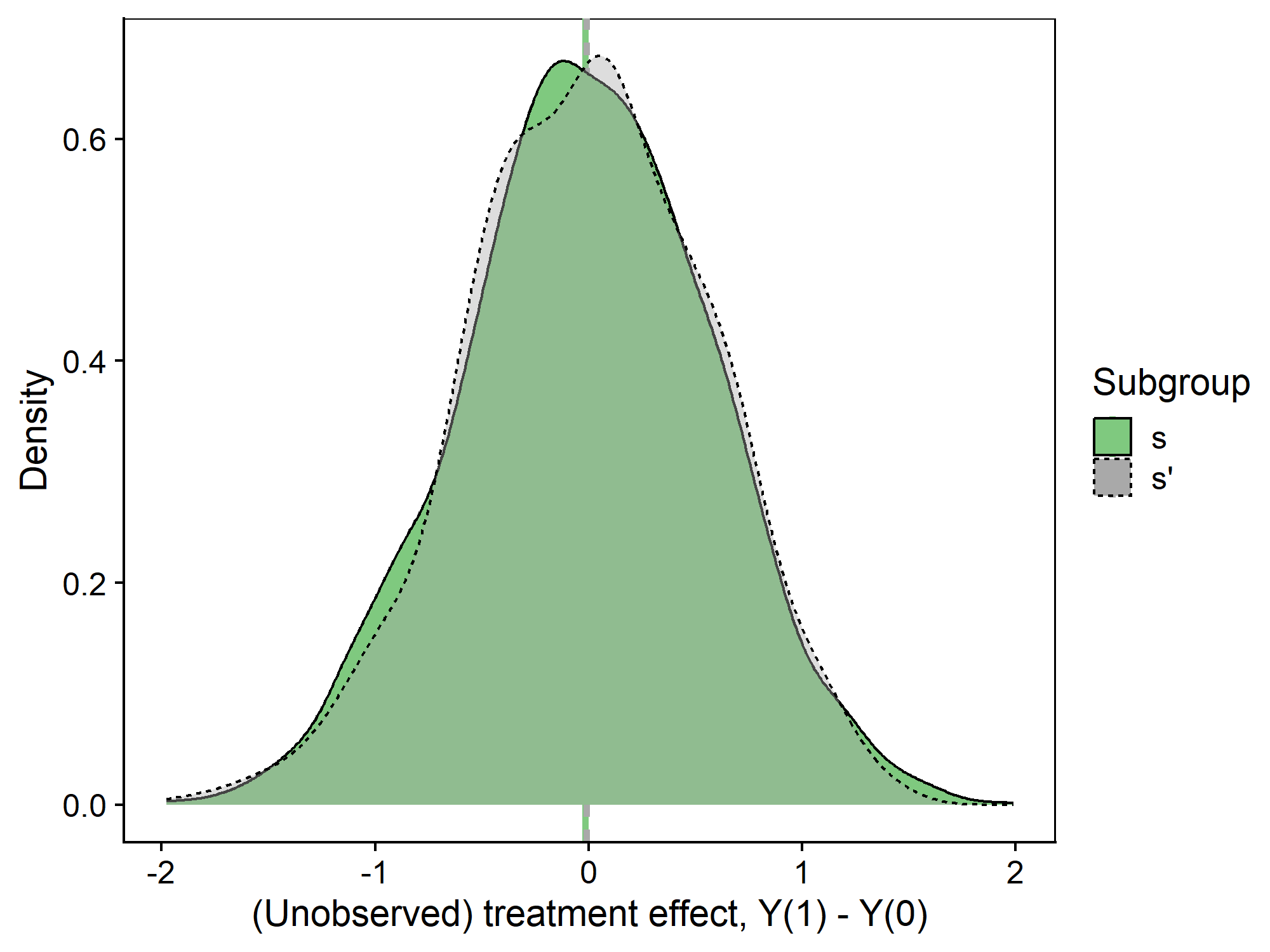
(a) No difference between subgroups

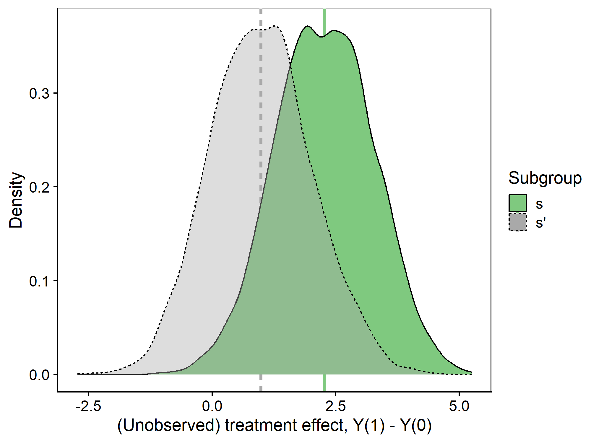
(b) $\gamma=0$

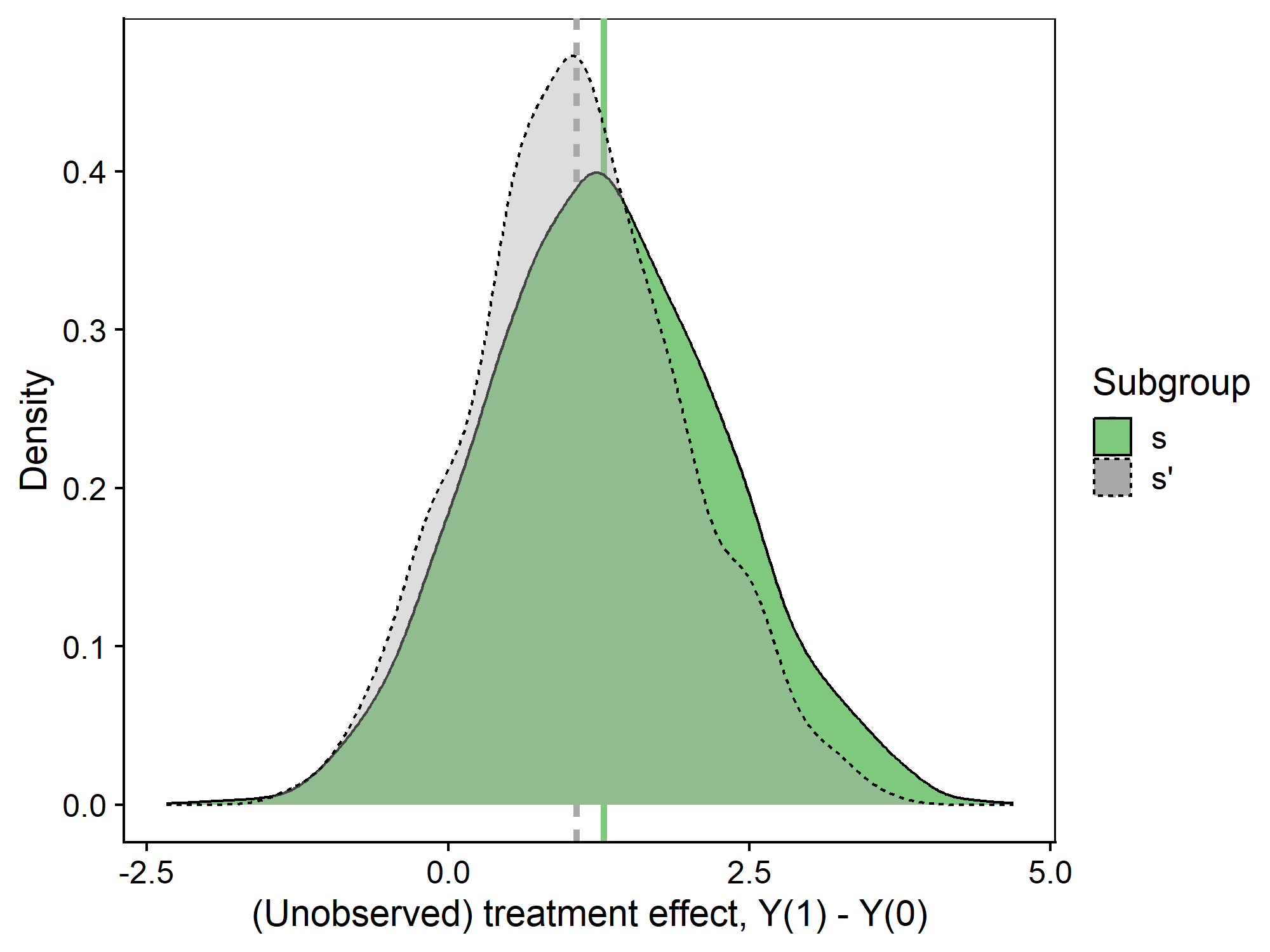
(c) $\gamma=0.2$

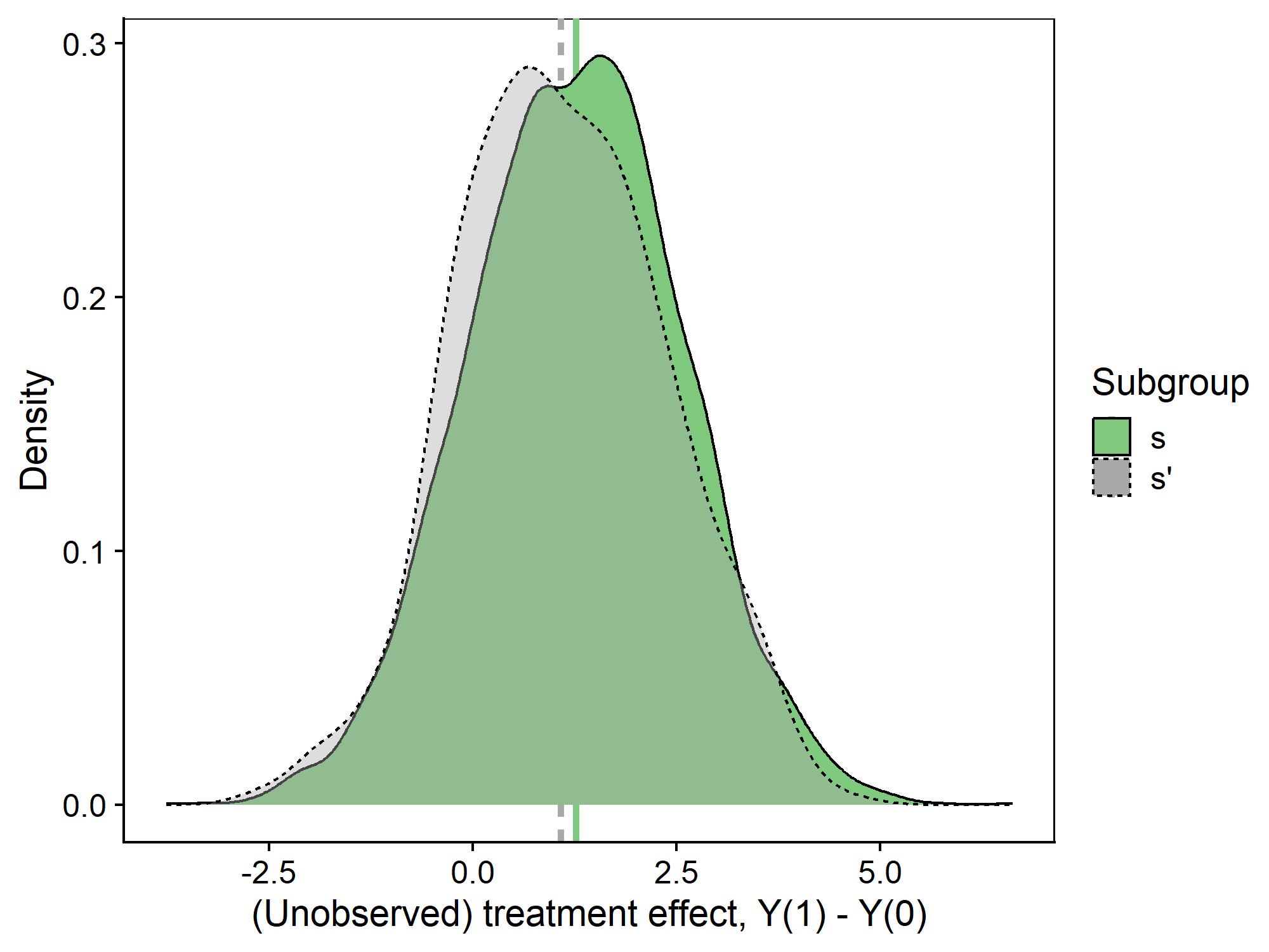
(d) $\gamma=1$

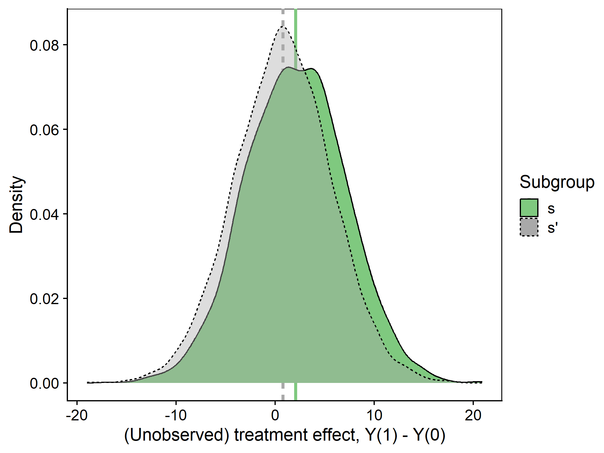
(e) $\gamma=5$

Notes: Vertical lines indicate the average treatment effect on the treated for each subgroup.

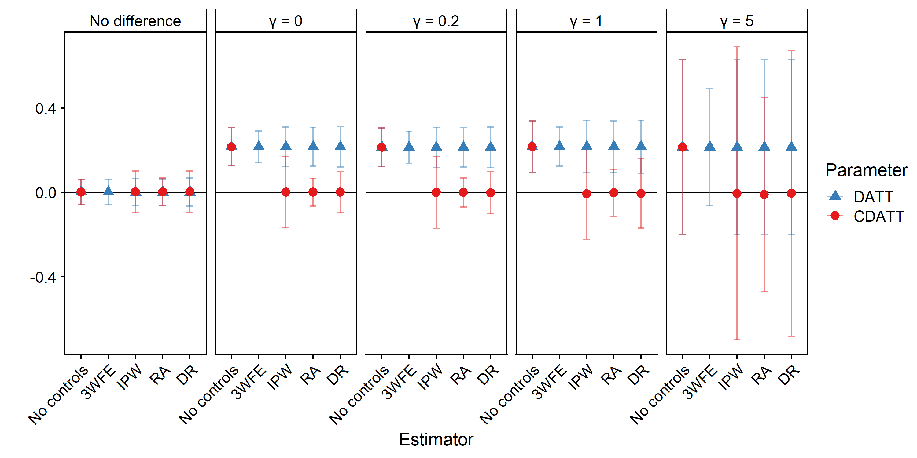
Figure 2: Estimator performance under various treatment effect heterogeneity scenarios

Notes: This figure presents the results of 1000 Monte Carlo simulations using the data-generating processes described above. The points represent the average value of the estimate across 1000 simulations. 95% confidence intervals are shown. “No difference” refers to a scenario with no average treatment effect, and no difference between subgroups.

First, the results underscore the divergence between the DATT and the CDATT when the underlying average treatment effects on the treated are correlated with subgroup status. When there is no difference in the treatment effects between the groups, the estimates of the DATT and CDATT are virtually identical. However, when the treatment effects vary with subgroup status, the DATT differs strongly from the CDATT. For example, an analysis of the DATT could lead a researcher to conclude that the treatment caused individuals in the targeted subgroup to experience an approximately 0.3 log point increase in wages relative to their untargeted counterparts. However, an analysis of the CDATT would highlight that this differential impact on the targeted subgroup was not causally due to their targeted-subgroup status, but rather explained by other factors, like age and education, that differ between the subgroups. The simulations make clear that, regardless of which estimator is used for the DATT, conditioning on covariates does not help the researcher recover an estimate of the CDATT.

Second, the results show that, as the variance in treatment effects increases, the estimators lose power and precision. When $\gamma=5$, the variance of the underlying treatment effects is large, and both estimators have substantially larger standard errors and confidence intervals relaive to the other scenarios. The loss in power is somewhat greater for the estimators of the CDATT due to the increased difficulty of distinguishing between the two groups. However, under moderate levels of treatment effect variance, the estimators of the CDATT have standard errors and confidence intervals on par with the DATT.

Table 1: Simulation study results based on 1000 Monte Carlo trials with $N=1000$

No average treatment effect on the treated
Estimator	Avg. bias	Med. bias	RMSE	SE	Cover	CI Len
No controls	0.001	0.001	0.032	0.031	0.943	0.120
$DATT^{3WFE}$	0.001	0.001	0.032	0.031	0.947	0.120
$DATT^{RA}$	0.001	0.000	0.032	0.032	0.944	0.124
$DATT^{IPW}$	0.001	0.001	0.034	0.033	0.949	0.131
$DATT^{DR}$	0.001	0.000	0.034	0.034	0.950	0.134
$CDATT^{RA}$	0.002	0.003	0.043	0.034	0.879	0.132
$CDATT^{IPW}$	0.003	0.003	0.052	0.050	0.937	0.197
$CDATT^{DR}$	0.003	0.003	0.052	0.050	0.929	0.196

$\mathbf{\gamma=0}$    Estimator Avg. bias Med. bias RMSE SE Cover CI Len No controls 0.216 0.216 0.221 0.046 0.005 0.182 $DATT^{3WFE}$ 0.216 0.216 0.221 0.038 0.002 0.150 $DATT^{RA}$ 0.216 0.216 0.221 0.047 0.007 0.184 $DATT^{IPW}$ 0.216 0.214 0.221 0.048 0.004 0.189 $DATT^{DR}$ 0.216 0.215 0.221 0.049 0.004 0.191 $CDATT^{RA}$ 0.001 0.003 0.043 0.034 0.876 0.132 $CDATT^{IPW}$ 0.001 0.003 0.074 0.086 0.977 0.339 $CDATT^{DR}$ 0.001 0.002 0.050 0.050 0.935 0.194   $\mathbf{\gamma=0.2}$    Estimator Avg. bias Med. bias RMSE SE Cover CI Len No controls 0.217 0.218 0.225 0.062 0.062 0.243 $DATT^{3WFE}$ 0.217 0.218 0.225 0.047 0.019 0.185 $DATT^{RA}$ 0.216 0.218 0.224 0.063 0.063 0.245 $DATT^{IPW}$ 0.217 0.218 0.225 0.063 0.071 0.249 $DATT^{DR}$ 0.216 0.218 0.224 0.064 0.070 0.250 $CDATT^{RA}$ -0.002 -0.001 0.073 0.057 0.876 0.225 $CDATT^{IPW}$ -0.006 -0.002 0.111 0.111 0.949 0.436 $CDATT^{DR}$ -0.005 -0.004 0.090 0.084 0.927 0.330   $\mathbf{\gamma=1}$    Estimator Avg. bias Med. bias RMSE SE Cover CI Len No controls 0.213 0.212 0.219 0.047 0.007 0.184 $DATT^{3WFE}$ 0.213 0.212 0.219 0.039 0.002 0.152 $DATT^{RA}$ 0.213 0.213 0.219 0.048 0.008 0.187 $DATT^{IPW}$ 0.213 0.212 0.219 0.049 0.012 0.191 $DATT^{DR}$ 0.213 0.214 0.219 0.049 0.011 0.194 $CDATT^{RA}$ -0.001 -0.002 0.044 0.035 0.878 0.137 $CDATT^{IPW}$ -0.000 0.003 0.079 0.087 0.969 0.342 $CDATT^{DR}$ -0.002 -0.001 0.053 0.051 0.937 0.201   $\mathbf{\gamma=5}$    Estimator Avg. bias Med. bias RMSE SE Cover CI Len No controls 0.215 0.219 0.299 0.212 0.825 0.829 $DATT^{3WFE}$ 0.215 0.219 0.299 0.142 0.599 0.556 $DATT^{RA}$ 0.215 0.221 0.299 0.212 0.832 0.830 $DATT^{IPW}$ 0.214 0.221 0.300 0.212 0.821 0.831 $DATT^{DR}$ 0.214 0.221 0.300 0.212 0.823 0.831 $CDATT^{RA}$ -0.010 -0.007 0.283 0.235 0.887 0.921 $CDATT^{IPW}$ -0.004 0.003 0.340 0.354 0.958 1.390 $CDATT^{DR}$ -0.005 0.000 0.332 0.345 0.954 1.353

Notes: This table presents the results of 1000 Monte Carlo simulations using the data-generating processes described above. Avg. bias refers to the average value of the estimate across 1000 simulations. Median bias refers to the median estimate. RMSE refers to the root mean squared error. Asym. SE refers to the average standard error across the trials. Cover refers to the 95% confidence interval coverage rate. CI Len refers to the average length of the 95% confidence interval.

Next, Table A.8 and Figure 3 compare the performance of the different estimators of the CDATT. The results highlight both the double-robustness of the doubly-robust estimator and its semiparametric efficiency.

Figure 3: Simulation study results based on 1000 Monte Carlo trials with $N=1000$

Notes: This figure presents the results of 1000 Monte Carlo simulations using the data-generating processes described above with $\gamma=1$. The points represent the average value of the estimate across 1000 simulations. 95% confidence intervals are shown.

The results show that the doubly-robust estimator of the CDATT performs well when at least one (but not necessarily both) set of working models is correctly specified. When both sets of working models are correctly specified, as in Case 1 in Table A.8, the regression adjustment, IPW, and doubly-robust estimators all perform well, with minimal bias. The doubly-robust estimator attains nearly correct coverage of the 95% confidence interval. When only the outcome regressions are specified correctly but the propensity scores are misspecified, as in Case 2, the regression adjustment and doubly-robust estimators have minimal bias, while the IPW estimator is biased. On the other hand, when the propensity score models are correct but the outcome regressions are misspecified, as in Case 3 and as expected, the IPW and doubly-robust methods are nearly unbiased, while the regression adjustment estimator has substantial bias. When all working models are misspecified, all available estimators have substantial bias and are not efficient.

The results also demonstrate the desirable performance of the doubly-robust estimator semiparameteric efficiency of the parameter. Across all cases, the standard error implied by the efficiency bound is 0.084. When both the propensity score models and the outcome regressions are correctly specified, the doubly-robust estimator achieves this efficiency bound. The regression adjustment estimator slightly outperforms the efficiency bound, while the IPW estimator is less efficient, a result paralleled by and discussed in [17]. When the outcome regressions are correcly specified, the doubly-robust estimator remains nearly as efficient as when the working models are correctly specified, this is not the case when the propensity score models are misspecified. For more details on doubly-robust estimators that are also asymptotically efficient under misspecification of either the propensity score or outcome model, see [17].

Table 2: Simulation study results under misspecification

Case 1: PS and OR correct
Estimator	Avg. bias	Med. bias	RMSE	Asym. SE	Cover	CI Len
No controls	0.214	0.216	0.223	0.062	0.071	0.243
$CDATT^{OR}$	0.000	0.002	0.071	0.057	0.881	0.225
$CDATT^{IPW}$	0.001	0.006	0.106	0.110	0.959	0.432
$CDATT^{DR}$	-0.002	0.000	0.087	0.083	0.944	0.326

Case 2: OR correct, PS incorrect    Estimator Avg. bias Med. bias RMSE Asym. SE Cover CI Len No controls 0.217 0.216 0.225 0.062 0.055 0.243 $CDATT^{OR}$ 0.002 0.002 0.073 0.057 0.876 0.225 $CDATT^{IPW}$ 0.275 0.274 0.283 0.066 0.016 0.258 $CDATT^{DR}$ 0.002 0.001 0.073 0.060 0.890 0.235   Case 3: PS correct, OR incorrect    Estimator Avg. bias Med. bias RMSE Asym. SE Cover CI Len No controls 0.216 0.215 0.225 0.062 0.059 0.243 $CDATT^{OR}$ 0.277 0.279 0.285 0.063 0.010 0.246 $CDATT^{IPW}$ 0.001 0.001 0.107 0.111 0.955 0.436 $CDATT^{DR}$ 0.001 0.003 0.107 0.111 0.954 0.436   Case 4: OR and PS incorrect    Estimator Avg. bias Med. bias RMSE Asym. SE Cover CI Len No controls 0.216 0.217 0.226 0.062 0.066 0.243 $CDATT^{OR}$ 0.277 0.278 0.285 0.063 0.018 0.246 $CDATT^{IPW}$ 0.275 0.275 0.283 0.066 0.027 0.258 $CDATT^{DR}$ 0.279 0.280 0.287 0.066 0.025 0.258

Notes: This table presents the results of 1000 Monte Carlo simulations using the data-generating processes described above with $\gamma=1$. Avg. bias refers to the average value of the estimate across 1000 simulations. Median bias refers to the median estimate. RMSE refers to the root mean squared error. Asym. SE refers to the average standard error across the trials. Cover refers to the 95% confidence interval coverage rate. CI Len refers to the average length of the 95% confidence interval.

5.4 Empirical approach for re-analysis of Gruber (1994)

As in the original paper, I use a triple difference design to estimate the impacts of coverage for maternity benefits on three subgroups of interest relative to a subgroup unlikely to use these benefits. I extend the analysis by implementing my proposed estimators of the CDATT.

The specification in the paper is as follows:

$$Y_{ijt}=\alpha+\beta_{1}X_{ijt}+\beta_{2}\tau_{t}+\beta_{3}\delta_{j}+\beta_{4}s_{i}+\beta_{5}(\delta_{j}\times\tau_{t})+\beta_{6}(\tau_{t}+s_{i})+\beta_{7}(\delta_{j}\times s_{i})+\beta_{8}(\delta_{j}\times\tau_{t}\times s_{i})$$

where $Y_{ijt}$ represents the outcome for individual $i$ in state $j$ in year $t$, $\delta_{j}$ represents state fixed effects, $\tau_{t}$ represents year fixed effects, and $s_{i}$ represents the demographic subgroup. Control variables are represented by $X_{ijt}$ and include education, experience and experience², sex, martial status, an interaction between sex and marital status, a binary variable for white/non-white, union/non-union, and indicators for 15 major industries. The coefficient of interest is given by $\beta_{8}$.

To motivate the inclusion of covariates and their role in this analysis, I first highlight the divergence between demographic groups in these covariates. Figure 4 shows, for example, that single women age 20-40 tend to have higher education than the other demographic groups, are more likely to be non-white, and are more likely to work in a white-collar job. This motivates the desire to separate between the DATT and CDATT parameters. If certain jobs, such as white-collar jobs, are more or less sensitive to the mandated benefits, then any difference in ATTs between the demographic groups might be explained by their different job characteristics rather than their gender, age, or marital status.

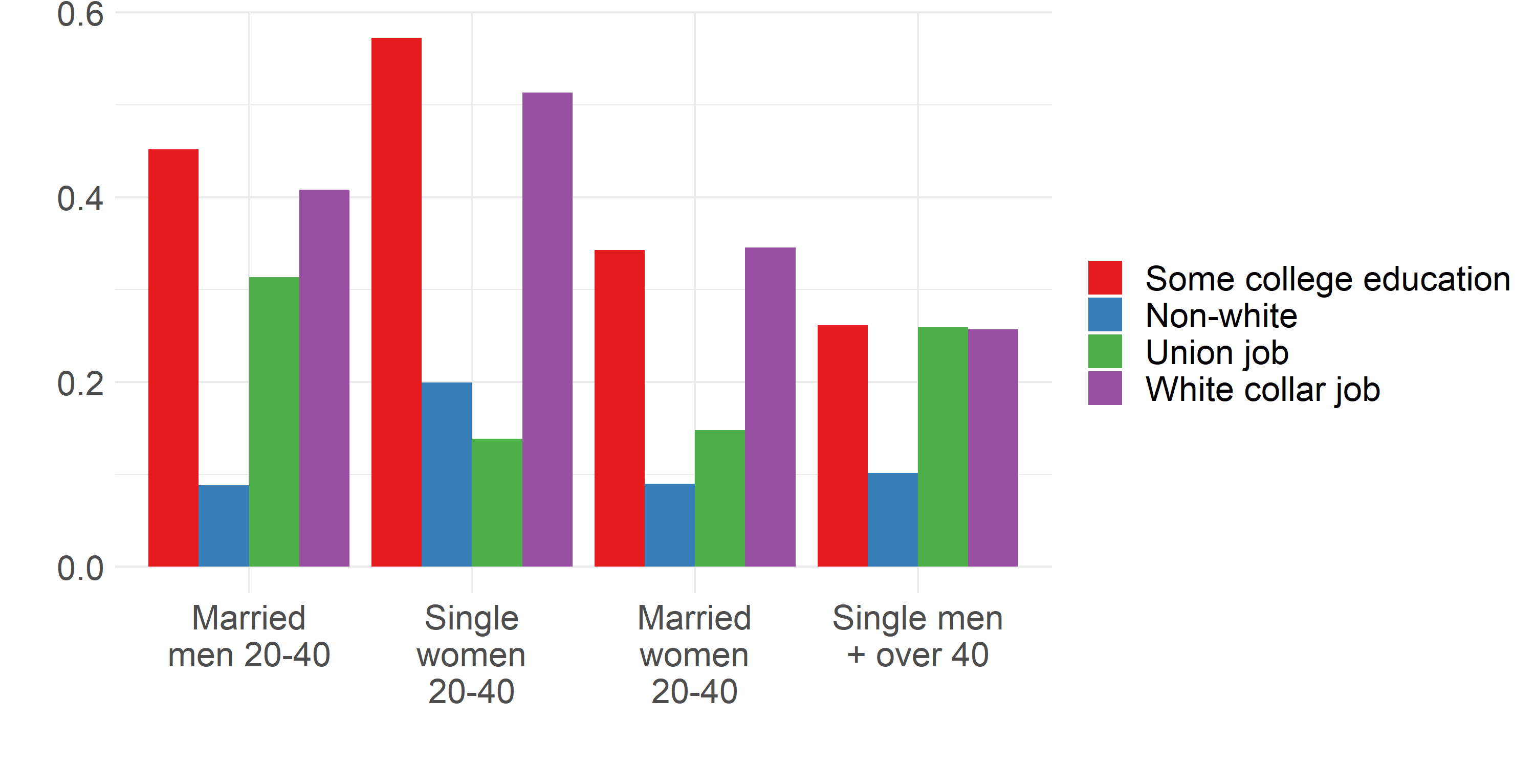
Figure 4: Descriptive statistics by subgroup

As described above, the DATT and the CDATT will coincide under the assumption of an unaffected subgroup. That is, if single men age 20-40 and people over age 40 are assumed to be entirely unaffected by the coverage of childbirth costs, then these two parameters will be equivalent. However, this assumption does not seem justified. For example, if the mandates make some workers more desirable (less costly) than others, then there will be spillovers on this untargeted group as employers substitute towards them. Further, if employers cannot pass on group-specific costs, then outcomes for all workers will be affected by the mandates.

In my analysis, I use the following covariates: education, a quadratic in age, white/non-white, union/non-union, and white-collar/not white-collar.

5.5 Results of Gruber (1994) re-analysis

Estimating the DATT, as in the published paper, I find that the impacts of mandating childbirth coverage differ between the targeted subgroups (married women age 20-40, married men age 20-40, and single women age 20-40). However, when estimating the CDATT, I find evidence that these differences between the subgroups should not be interpreted as caused by subgroup status, but instead appear to be due to differences in covariates between the groups.

Figure 5(a) highlights that, when estimating the DATT on the log of hourly wages, results are consistent with the original published results, regardless of which triple difference estimator is used. When not including controls, the CDATT and the DATT coincide. When using a 3WFE design similar to that in the original paper, the results suggest an impact of -0.009, -0.039, and -0.074 log points in wages for married men age 20-40, married women age 20-40, and single women age 20-40, respectively. These estimates are similar to those presented in the original paper, which suggested impacts of -0.009, -0.043, and -0.042 for these groups, respectively (see Table 4 in [9]). When including controls using the doubly robust estimator, the magnitudes of the estimates of the DATT are largely unchanged, but somewhat less precisely estimated. These estimates suggest a reduction in wages for all targeted groups, which is significant regardless of estimator for single women age 20-40. The published result found significant declines for both married women age 20-40 and single women age 20-40.

Although analysis of the DATT suggests that the benefits mandates reduced wages for the targeted subgroups relative to the untargeted subgroup, the CDATT suggests this may not be causally due to subgroup status. Figure 5(a) shows how the estimates of the CDATT diverge from the DATT. For married men, the doubly-robust estimate is large and positive (although insignificant). For married women, it is slightly positive (insignificant), and for single women, it is slightly negative (insignificant). Although the DATT is consistently negative for all three groups, the CDATT offers a qualitatively different result.

Turning to the impacts on hours worked, the DATT and the CDATT again may have different interpretations. For married men age 20-40, the 3WFE specification reveals a significant increase in hours worked per week, by about 0.042 log points (compared to the published estimate of 0.030 log points). The magnitude of this impact is similar when including controls via the doubly-robust estimator of the DATT (0.029 log points, very similar to the published result). However, it is just as large but negative when estimating the CDATT using the doubly-robust estimator, with a magnitude of -0.030 (insignificant). For married women, again, both estimates of the DATT reveal a positive impact of 0.058 and 0.060 log points (compared to the published impact of 0.049 log points). However, the estimate of the CDATT is smaller, only 0.031 log points, and insignificant. Finally, there is no significant impact in any case for single women, as in the published results.

The results on employment suggest much less divergence between the two estimators, and weaker overall evidence of an impact. As in the published paper, estimates of the DATT are generally negative and insignificant. However, it is not surprising that the DATT and CDATT diverge less in this case. The difference between the two arises when treatment effects are correlated with subgroup status, and, if treatment effects are truly small or null, the magnitude of the difference between subgroups will be smaller.

Figure 5: Results from re-analyzing impacts of childbirth coverage

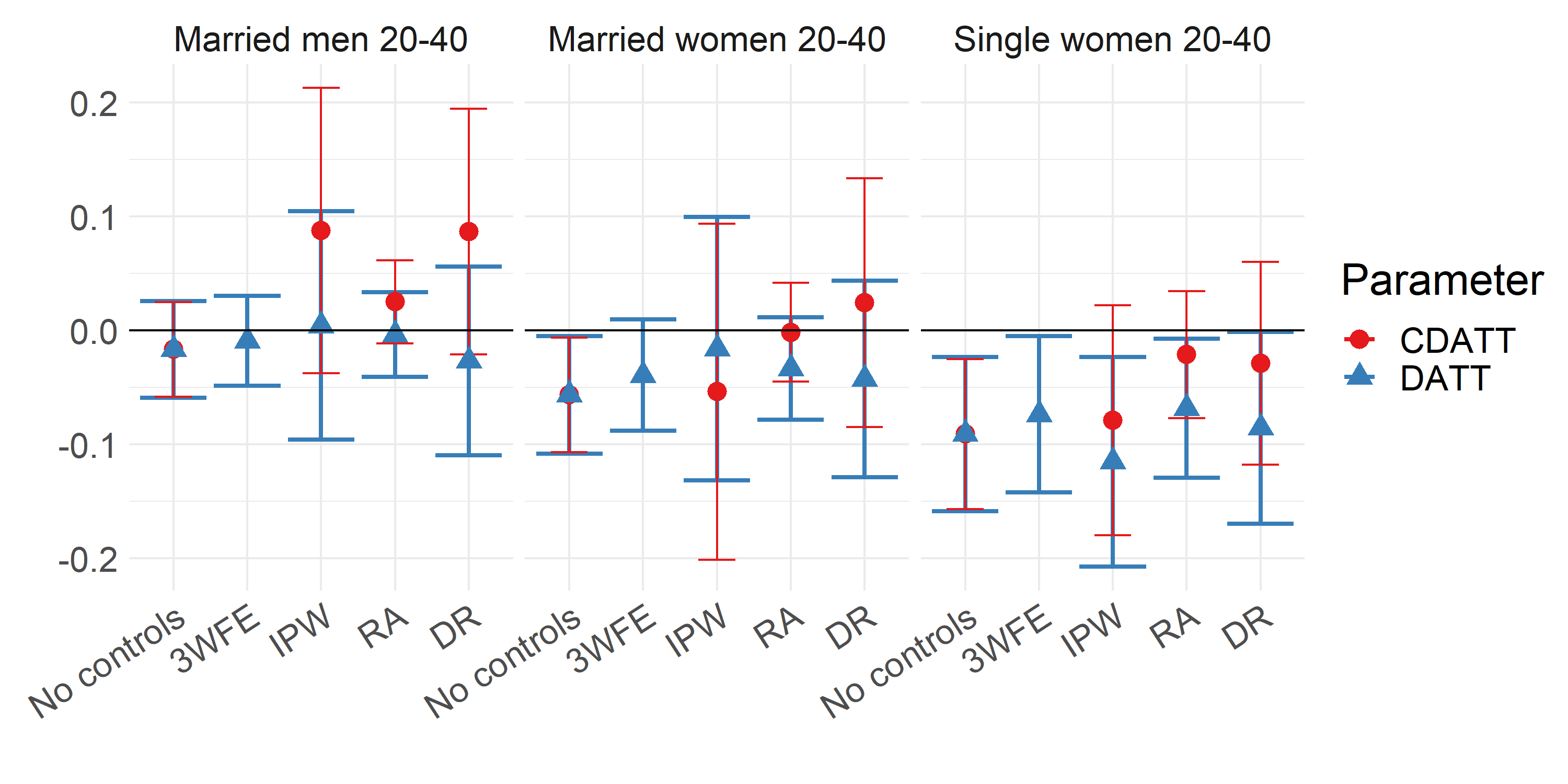
(a) Impacts on log of hourly wages

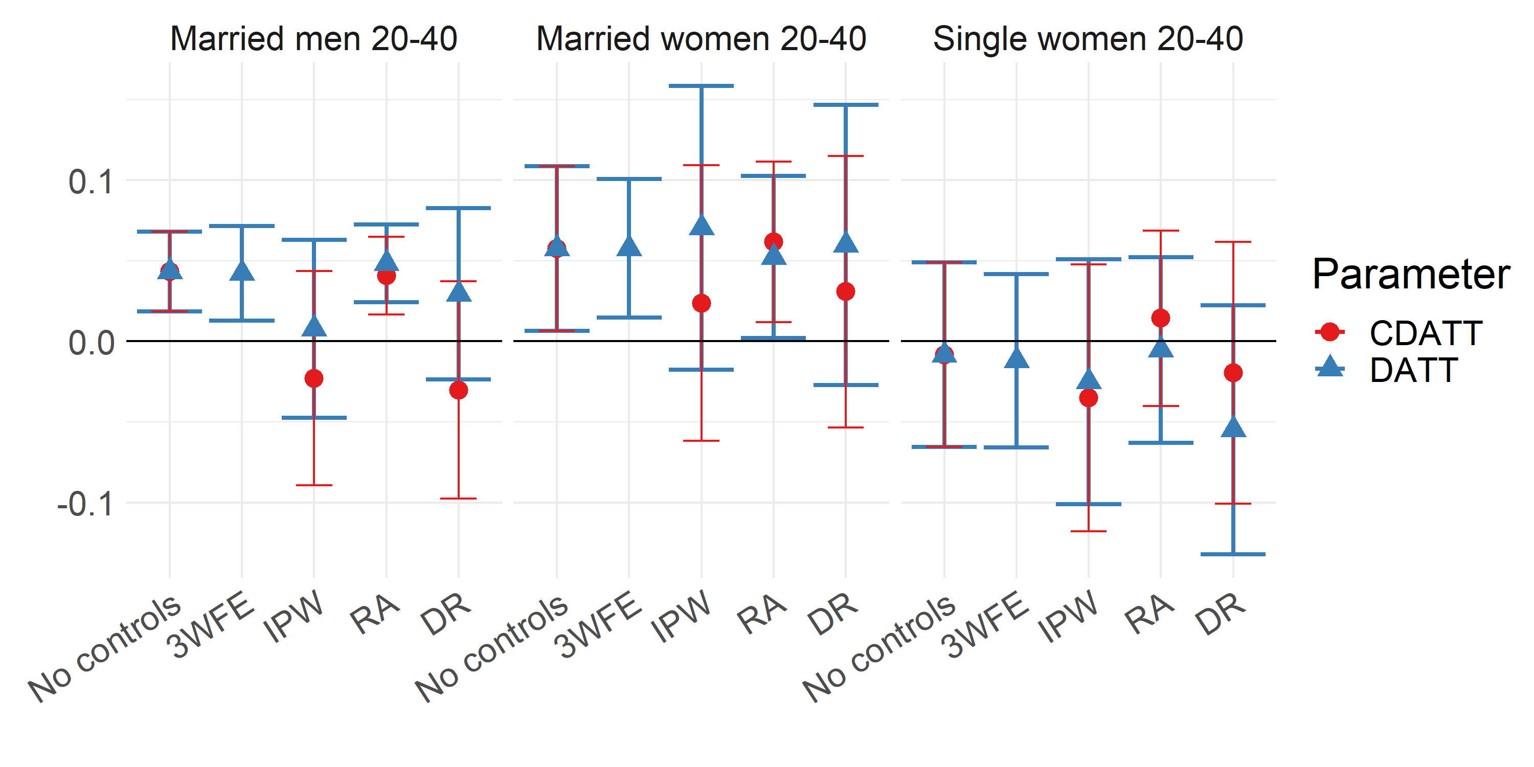
(b) Impacts on log of hours worked

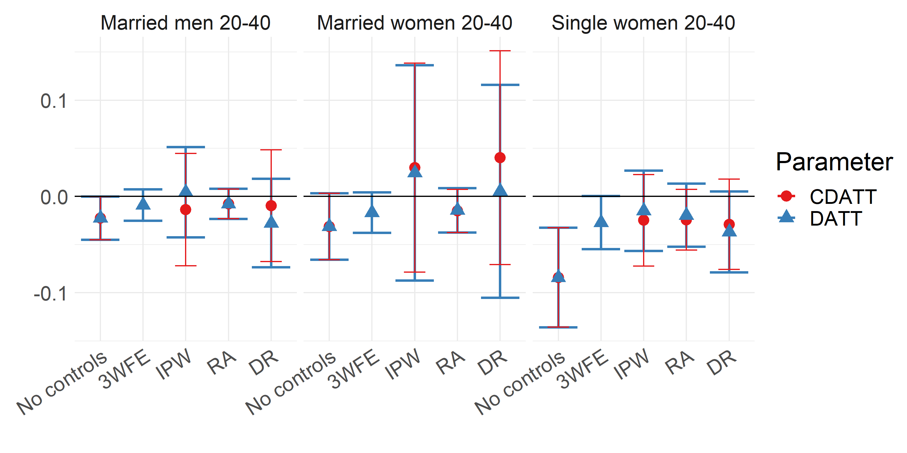
(c) Impacts on employment

6 Conclusion

In this paper, I have addressed identification and estimation in triple difference designs when treatment effects are heterogeneous. I begin by discussing two parameters of interest, the difference in ATTs between subgroups (DATT) and the causal difference in ATTs between subgroups (CDATT). When treatment effects are heterogeneous, these two parameters may differ in important ways, and caution is warranted to avoid interpreting a DATT as a CDATT.

I show that the DATT can be identified under an assumption on the trend in the gap between subgroups’ outcomes. I highlight that the ATT can be recovered only under the assumption of a subgroup that is unaffected by the treatment. I then show that identification of the CDATT requires additional assumptions on treatment effect heterogeneity, for example, the assumption that treatment effect heterogeneity is captured by observable characteristics.

Next, I derive the semiparametric efficiency bounds for the CDATT, and propose estimators for it. I discuss their asymptotic properties and show that these estimators achieve semiparametric efficiency. A realistic simulation study calibrated to the application in [9] highlights these results. The simulations first highlight the divergence between the DATT and the CDATT, and show that estimators for the DATT can provide misleading results if they are interpreted causally in cases where subgroups differ in their sensitivity to the treatment. They also show that the proposed estimators for the CDATT are unbiased and perform well in finite samples.

An application of these estimators to the analysis in [9] highlights a case where heterogeneity in sensitivity to a treatment can correlate with subgroup status, affecting the interpretation of the triple difference estimates. The analysis addresses the question of whether employers can pass on group-specific costs on the basis of demographic characteristics. The paper uses a triple difference design to study the impacts of state-level mandates requiring insurance to cover costs for childbirth. Since these benefits are likely to be used by certain groups (ie, women age 20-40 and married men age 20-40), the triple difference design allows to test for differential effects for this group relative to other segments of the population. Although an analysis of the DATT suggests that there is significant differential cost-shifting for these groups, estimating the CDATT offers little evidence that this difference is causal on the basis of demographic characteristics. Researchers should take treatment effect heterogeneity into account in the interpretation and estimation of treatment effects in triple difference designs.

Appendix A Proofs of results for panel data

A.1 Identification

Proof A.1.

Proof of Proposition 1: Identification of $DATT_{s-s^{\prime}}(g,t)$ in the staggered case, with not-yet-treated units used for comparison.

$$D ATT_{s-s^{\prime}}(g,t)$$

$$= \mathbb{E}[Y_{t}(g)-Y_{t}(\infty)|G=g,S=s]-\mathbb{E}[Y_{t}(g)-Y_{t}(\infty)|G=g,S=s^{\prime}]$$

$$= \mathbb{E}[Y_{t}(g)-Y_{t}(\infty)|G=g,S=s]-\mathbb{E}[Y_{t}(g)-Y_{t}(\infty)|G=g,S=s^{\prime}]$$

$$+\mathbb{E}\Big{[}Y_{t}(\infty)-Y_{g-1}(\infty)|G=g,S=s\Big{]}-\mathbb{E}\Big{[}Y_{t}(\infty)-Y_{g-1}(\infty)|G=g,S=s^{\prime}\Big{]}$$

$$-\Big{(}\mathbb{E}\Big{[}Y_{t}(\infty)-Y_{g-1}(\infty)|W_{t}=0,G\neq g,S=s\Big{]}-\mathbb{E}\Big{[}Y_{t}(\infty)-Y_{g-1}(\infty)|W_{t}=0,G\neq g,S=s^{\prime}\Big{]}\Big{)}$$

$$= \mathbb{E}[Y_{t}(g)-Y_{g-1}(\infty)|G=g,S=s]-\mathbb{E}[Y_{t}(g)-Y_{g-1}(\infty)|G=g,S=s^{\prime}]$$

$$-\Big{(}\mathbb{E}\Big{[}Y_{t}(\infty)-Y_{g-1}(\infty)|W_{t}=0,G\neq g,S=s\Big{]}-\mathbb{E}\Big{[}Y_{t}(\infty)-Y_{g-1}(\infty)|W_{t}=0,G\neq g,S=s^{\prime}\Big{]}\Big{)}$$

$$= \mathbb{E}[Y_{t}-Y_{g-1}|G=g,S=s]-\mathbb{E}[Y_{t}-Y_{g-1}|G=g,S=s^{\prime}]$$

$$-\Big{(}\mathbb{E}[Y_{t}-Y_{g-1}|W_{t}=0,G\neq g,S=s]-\mathbb{E}[Y_{t}-Y_{g-1}|W_{t}=0,G\neq g,S=s^{\prime}]\Big{)}$$

where the first equality follows from the definition of the $DATT_{s-s^{\prime}}(g,t)$, the second follows from Assumption 3 with degenerate $X$ for time periods $t\geq g$, the third from combining terms, and the last from Assumption 2.

Proof A.2.

Proof of Proposition 1: Identification of $DATT_{s-s^{\prime}}(g,t)$ in the staggered case, with never-treated units used for comparison.

$$DATT_{s-s^{\prime}}(g,t)$$

$$= \mathbb{E}[Y_{t}(g)-Y_{t}(\infty)|G=g,S=s]-\mathbb{E}[Y_{t}(g)-Y_{t}(\infty)|G=g,S=s^{\prime}]$$

$$= \mathbb{E}[Y_{t}(g)-Y_{t}(\infty)|G=g,S=s]-\mathbb{E}[Y_{t}(g)-Y_{t}(\infty)|G=g,S=s^{\prime}]$$

$$+\mathbb{E}\Big{[}Y_{t}(\infty)-Y_{g-1}(\infty)|G=g,S=s\Big{]}-\mathbb{E}\Big{[}Y_{t}(\infty)-Y_{g-1}(\infty)|G=g,S=s^{\prime}\Big{]}$$

$$-\Big{(}\mathbb{E}\Big{[}Y_{t}(\infty)-Y_{g-1}(\infty)|G=\infty,S=s\Big{]}-\mathbb{E}\Big{[}Y_{t}(\infty)-Y_{g-1}(\infty)|G=\infty,S=s^{\prime}\Big{]}\Big{)}$$

$$= \mathbb{E}[Y_{t}(g)-Y_{g-1}(\infty)|G=g,S=s]-\mathbb{E}[Y_{t}(g)-Y_{g-1}(\infty)|G=g,S=s^{\prime}]$$

$$-\Big{(}\mathbb{E}\Big{[}Y_{t}(\infty)-Y_{g-1}(\infty)|G=\infty,S=s\Big{]}-\mathbb{E}\Big{[}Y_{t}(\infty)-Y_{g-1}(\infty)|G=\infty,S=s^{\prime}\Big{]}\Big{)}$$

$$= \mathbb{E}[Y_{t}-Y_{g-1}|G=g,S=s]-\mathbb{E}[Y_{t}-Y_{g-1}|G=g,S=s^{\prime}]$$

$$-\Big{(}\mathbb{E}[Y_{t}-Y_{g-1}|G=\infty,S=s]-\mathbb{E}[Y_{t}-Y_{g-1}|G=\infty,S=s^{\prime}]\Big{)}$$

where the first equality follows from the definition of the $DATT_{s-s^{\prime}}(g,t)$, the second follows from Assumption 4 with degenerate $X$ for time periods $t\geq g$, the third from combining terms, and the last from the definitions of the potential and observed outcomes and Assumption 2.

When conditioning on $X$, the results follow from those in [4].

Proof A.3.

Proof of Proposition 2: Identification of $CDATT_{s-s^{\prime}}(g,t)$ in the staggered case with not-yet-treated group as comparison.

$$C DATT_{s-s^{\prime}}(g,t)$$

$$= \mathbb{E}[Y_{t}(g;s)-Y_{t}(\infty;s)|G=g,S=s]-\mathbb{E}[Y_{t}(g;s^{\prime})-Y_{t}(\infty;s^{\prime})|G=g,S=s]$$

$$= \mathbb{E}[Y_{t}(g)-Y_{t}(\infty)|G=g,S=s]-\mathbb{E}[Y_{t}(g)-Y_{t}(\infty)|G=g,S=s^{\prime}]$$

$$= \mathbb{E}[Y_{t}(g)-Y_{t}(\infty)|G=g,S=s]-\mathbb{E}[Y_{t}(g)-Y_{t}(\infty)|G=g,S=s^{\prime}]$$

$$+\mathbb{E}\Big{[}Y_{t}(\infty)-Y_{g-1}(\infty)|G=g,S=s\Big{]}-\mathbb{E}\Big{[}Y_{t}(\infty)-Y_{g-1}(\infty)|G=g,S=s^{\prime}\Big{]}$$

$$-\Big{(}\mathbb{E}\Big{[}Y_{t}(\infty)-Y_{g-1}(\infty)|W_{t}=0,G\neq g,S=s\Big{]}-\mathbb{E}\Big{[}Y_{t}(\infty)-Y_{g-1}(\infty)|W_{t}=0,G\neq g,S=s^{\prime}\Big{]}\Big{)}$$

$$= \mathbb{E}[Y_{t}(g)-Y_{g-1}(\infty)|G=g,S=s]-\mathbb{E}[Y_{t}(g)-Y_{g-1}(\infty)|G=g,S=s^{\prime}]$$

$$-\Big{(}\mathbb{E}\Big{[}Y_{t}(\infty)-Y_{g-1}(\infty)|W_{t}=0,G\neq g,S=s\Big{]}-\mathbb{E}\Big{[}Y_{t}(\infty)-Y_{g-1}(\infty)|W_{t}=0,G\neq g,S=s^{\prime}\Big{]}\Big{)}$$

$$= \mathbb{E}[Y_{t}-Y_{g-1}|G=g,S=s]-\mathbb{E}[Y_{t}-Y_{g-1}|G=g,S=s^{\prime}]$$

$$-\Big{(}\mathbb{E}[Y_{t}-Y_{g-1}|W_{t}=0,G\neq g,S=s]-\mathbb{E}[Y_{t}-Y_{g-1}|W_{t}=0,G\neq g,S=s^{\prime}]\Big{)}$$

where the first equality follows from the definition of $CDATT_{s-s^{\prime}}(g,t)$, the second from Assumption 6, the third from Assumption 3, the fourth from combining and simplifying terms as above, and the last from Assumption 2.

Proof A.4.

Proof of Proposition 2: Identification of $CDATT_{s-s^{\prime}}(g,t)$ in the staggered case with never-treated group as comparison

$$CDATT_{s-s^{\prime}}(g,t)$$

$$= \mathbb{E}[Y_{t}(g;s)-Y_{t}(\infty;s)|G=g,S=s]-\mathbb{E}[Y_{t}(g;s^{\prime})-Y_{t}(\infty;s^{\prime})|G=g,S=s]$$

$$= \mathbb{E}[Y_{t}(g)-Y_{t}(\infty)|G=g,S=s]-\mathbb{E}[Y_{t}(g)-Y_{t}(\infty)|G=g,S=s^{\prime}]$$

$$= \mathbb{E}[Y_{t}(g)-Y_{t}(\infty)|G=g,S=s]-\mathbb{E}[Y_{t}(g)-Y_{t}(\infty)|G=g,S=s^{\prime}]$$

$$+\mathbb{E}\Big{[}Y_{t}(\infty)-Y_{g-1}(\infty)|G=g,S=s\Big{]}-\mathbb{E}\Big{[}Y_{t}(\infty)-Y_{g-1}(\infty)|G=g,S=s^{\prime}\Big{]}$$

$$-\Big{(}\mathbb{E}\Big{[}Y_{t}(\infty)-Y_{g-1}(\infty)|G=\infty,S=s\Big{]}-\mathbb{E}\Big{[}Y_{t}(\infty)-Y_{g-1}(\infty)|G=\infty,S=s^{\prime}\Big{]}\Big{)}$$

$$= \mathbb{E}[Y_{t}(g)-Y_{g-1}(\infty)|G=g,S=s]-\mathbb{E}[Y_{t}(g)-Y_{g-1}(\infty)|G=g,S=s^{\prime}]$$

$$-\Big{(}\mathbb{E}\Big{[}Y_{t}(\infty)-Y_{g-1}(\infty)|G=\infty,S=s\Big{]}-\mathbb{E}\Big{[}Y_{t}(\infty)-Y_{g-1}(\infty)|G=\infty,S=s^{\prime}\Big{]}\Big{)}$$

$$= \mathbb{E}[Y_{t}-Y_{g-1}|G=g,S=s]-\mathbb{E}[Y_{t}-Y_{g-1}|G=g,S=s^{\prime}]$$

$$-\Big{(}\mathbb{E}[Y_{t}-Y_{g-1}|G=\infty,S=s]-\mathbb{E}[Y_{t}-Y_{g-1}|G=\infty,S=s^{\prime}]\Big{)}$$

where the first equality follows from the definition of $CDATT_{s-s^{\prime}}(g,t)$, the second from Assumption 6, the third from Assumption 3, the fourth from combining and simplifying terms as above, and the last from Assumption 2.

Proof A.5.

To show $CDATT^{IPW,c}_{s-s^{\prime}}(g,t)=CDATT_{s-s^{\prime}}(g,t)$.

First, we can show that

$$\mathbb{E}\Big{[}\Big{(}\frac{G_{g}S_{s}}{\mathbb{E}[G_{g}S_{s}]}\Big{)}(Y_{t}-Y_{g-1})\Big{]} =\frac{\mathbb{E}[G_{g}S_{s}]\mathbb{E}[Y_{t}-Y_{g-1}|G_{g}=1,S_{s}=1]}{\mathbb{E}[G_{g}S_{s}]}$$

$$=\mathbb{E}[Y_{t}-Y_{g-1}|G_{g}=1,S_{s}=1]$$

(using Assumption 2) $$=\mathbb{E}[Y_{t}(g;s)-Y_{g-1}(\infty;s)|G_{g}=1,S_{s}=1]$$

Using a similar argument and the law of iterated expectations,

$$\mathbb{E}\Big{[}\Big{(}\frac{\pi_{g,s}(X)C_{c}S_{s}}{\pi_{c,s}(X)\mathbb{E}[C_{c}S_{s}]}\Big{)}(Y_{t}-Y_{g-1})\Big{]} =\mathbb{E}\Big{[}\frac{\mathbb{E}[G_{g}S_{s}|X]\mathbb{E}[C_{c}S_{s}(Y_{t}-Y_{g-1})|X]}{\mathbb{E}[C_{c}S_{s}|X]\mathbb{E}[G_{g}S_{s}]}\Big{]}$$

$$=\mathbb{E}\Big{[}\frac{\mathbb{E}[G_{g}S_{s}|X]\mathbb{E}[C_{c}S_{s}|X]\mathbb{E}[Y_{t}-Y_{g-1}|X,C_{c}=1,S_{s}=1]}{\mathbb{E}[C_{c}S_{s}|X]\mathbb{E}[G_{g}S_{s}]}\Big{]}$$

$$=\mathbb{E}\Big{[}\mathbb{E}[Y_{t}(\infty;s)-Y_{g-1}(\infty;s)|X,C_{c}=1,S_{s}=1]\Big{]}$$

By the same process,

$$\mathbb{E}\Big{[}\Big{(}\frac{\pi_{g,s}(X)G_{g}S_{s^{\prime}}}{\pi_{g,s^{\prime}}(X)\mathbb{E}[G_{g}S_{s}]}\Big{)}(Y_{t}-Y_{g-1})\Big{]} =\mathbb{E}\Big{[}\frac{\mathbb{E}[G_{g}S_{s}|X]\mathbb{E}[G_{g}S_{s^{\prime}}(Y_{t}-Y_{g-1})|X]}{\mathbb{E}[G_{g}S_{s^{\prime}}|X]\mathbb{E}[G_{g}S_{s}]}\Big{]}$$

$$=\mathbb{E}\Big{[}\frac{\mathbb{E}[G_{g}S_{s}|X]\mathbb{E}[G_{g}S_{s^{\prime}}|X]\mathbb{E}[Y_{t}-Y_{g-1}|X,G_{g}=1,S_{s^{\prime}}=1]}{\mathbb{E}[G_{g}S_{s^{\prime}}|X]\mathbb{E}[G_{g}S_{s}]}\Big{]}$$

$$=\mathbb{E}\Big{[}\mathbb{E}[Y_{t}(g;s^{\prime})-Y_{g-1}(\infty;s^{\prime})|X,G_{g}=1,S_{s^{\prime}}=1]\Big{]}$$

(using Assumption 7) $$=\mathbb{E}\Big{[}\mathbb{E}[Y_{t}(g;s^{\prime})-Y_{g-1}(\infty;s^{\prime})|X,G_{g}=1,S_{s}=1]\Big{]}$$

$$=\mathbb{E}[Y_{t}(g;s^{\prime})-Y_{g-1}(\infty;s^{\prime})|G_{g}=1,S_{s}=1]$$

By the same process and using Assumption 7 again,

$$\mathbb{E}\Big{[}\Big{(}\frac{\pi_{g,s}(X)C_{c}S_{s^{\prime}}}{\pi_{c,s^{\prime}}(X)\mathbb{E}[C_{c}S_{s}]}\Big{)}(Y_{t}-Y_{g-1})\Big{]} =\mathbb{E}[Y_{t}(\infty;s^{\prime})-Y_{g-1}(\infty;s^{\prime})|C_{c}=1,S_{s}=1]$$

Applying Assumption 3 or 4, conditional on $X$, finishes the proof:

$$\mathbb{E} [Y_{t}(g;s)-Y_{g-1}(\infty;s)|G_{g}=1,S_{s}=1]-\mathbb{E}\Big{[}\mathbb{E}[Y_{t}(\infty;s)-Y_{g-1}(\infty;s)|X,C_{c}=1,S_{s}=1]\Big{]}$$

$$-\Big{(}\mathbb{E}[Y_{t}(g;s^{\prime})-Y_{g-1}(\infty;s^{\prime})|G_{g}=1,S_{s}=1]-\mathbb{E}\Big{[}\mathbb{E}[Y_{t}(\infty;s^{\prime})-Y_{g-1}(\infty;s^{\prime})|X,C_{c}=1,S_{s}=1]\Big{]}\Big{)}$$

$$= \mathbb{E}[Y_{t}(g;s)-Y_{g-1}(\infty;s)|G_{g}=1,S_{s}=1]-\mathbb{E}\Big{[}\mathbb{E}[Y_{t}(\infty;s)-Y_{g-1}(\infty;s)|X,G_{g}=1,S_{s}=1]\Big{]}$$

$$-\Big{(}\mathbb{E}[Y_{t}(g;s^{\prime})-Y_{g-1}(\infty;s^{\prime})|G_{g}=1,S_{s}=1]-\mathbb{E}\Big{[}\mathbb{E}[Y_{t}(\infty;s^{\prime})-Y_{g-1}(\infty;s^{\prime})|X,G_{g}=1,S_{s}=1]\Big{]}\Big{)}$$

$$= \mathbb{E}[Y_{t}(g;s)-Y_{t}(\infty;s)|G_{g}=1,S_{s}=1]-\Big{(}\mathbb{E}[Y_{t}(g;s^{\prime})-Y_{t}(\infty;s^{\prime})|G_{g}=1,S_{s}=1]\Big{)}$$

$$= CDATT_{s-s^{\prime}}(g,t)$$

Proof A.6.

To show $CDATT^{RA,c}_{s-s^{\prime}}(g,t)=CDATT_{s-s^{\prime}}(g,t)$.

First note that, under Assumptions 1 and 2,

$$\mathbb{E}\Big{[}\frac{G_{g}S_{s}}{\mathbb{E}[G_{g}S_{s}]}(Y_{t}-Y_{g-1})\Big{]}=\mathbb{E}[Y_{t}(g;s)-Y_{g-1}(\infty;s)|G=g,S=s]$$

Similarly,

$$\mathbb{E}\Big{[}\frac{G_{g}S_{s}}{\mathbb{E}[G_{g}S_{s}]}(Y_{t}-Y_{g-1})\Big{]} =\mathbb{E}[Y_{t}(\infty;s)-Y_{g-1}(\infty;s)|C_{c}=1,S=s]$$

Next, using Assumption 7,

$$\mathbb{E}\Big{[}\frac{G_{g}S_{s}}{\mathbb{E}[G_{g}S_{s}]}\mu_{g,t}^{s^{\prime}}(x)\Big{]} =\mathbb{E}\Big{[}\frac{G_{g}S_{s}}{\mathbb{E}[G_{g}S_{s}]}\mathbb{E}[Y_{t}(g;s^{\prime})-Y_{g-1}(\infty;s^{\prime})|G=g,S=s^{\prime},X=x]\Big{]}$$

$$=\mathbb{E}[Y_{t}(g;s^{\prime})-Y_{g-1}(\infty;s^{\prime})|G=g,S=s]$$

$$\mathbb{E}\Big{[}\frac{G_{g}S_{s}}{\mathbb{E}[G_{g}S_{s}]}\mu_{c,g,t}^{s^{\prime}}(x)\Big{]} =\mathbb{E}\Big{[}\frac{G_{g}S_{s}}{\mathbb{E}[G_{g}S_{s}]}\mathbb{E}[Y_{t}(\infty;s^{\prime})-Y_{g-1}(\infty;s^{\prime})|C_{c}=1,S=s^{\prime},X=x]\Big{]}$$

$$=\mathbb{E}[Y_{t}(\infty;s^{\prime})-Y_{g-1}(\infty;s^{\prime})|C_{c}=1,S=s]$$

Applying Assumption 3 or 4, conditional on $X$, finishes the proof.

Proof A.7.

To show $CDATT^{DR,c}_{s-s^{\prime}}(g,t)=CDATT_{s-s^{\prime}}(g,t)$, first note that

$$\mathbb{E} \Big{[}\Big{(}w_{1}(G_{g},S_{s})-w_{2}(G_{g},S_{s^{\prime}},X)\Big{)}\mu_{g,t}^{s^{\prime}}(X)\Big{]}$$

$$=\mathbb{E}\Big{[}\Big{(}\frac{G_{g}S_{s}}{\mathbb{E}[G_{g}S_{s}]}-\frac{G_{g}S_{s^{\prime}}\pi_{g,s}(X)}{\pi_{g,s^{\prime}}(X)}\Big{/}\mathbb{E}\Big{[}\frac{G_{g}S_{s^{\prime}}\pi_{g,s}(X)}{\pi_{g,s^{\prime}}(X)}\Big{]}\Big{)}\mu_{g,t}^{s^{\prime}}(X)\Big{]}$$

$$=\mathbb{E}\Big{[}\Big{(}\frac{G_{g}S_{s}}{\mathbb{E}[G_{g}S_{s}]}-\frac{G_{g}S_{s^{\prime}}\mathbb{E}[G_{g}S_{s}|X]}{\mathbb{E}[G_{g}S_{s^{\prime}}|X]}\Big{/}\mathbb{E}\Big{[}\frac{G_{g}S_{s^{\prime}}\mathbb{E}[G_{g}S_{s}|X]}{\mathbb{E}[G_{g}S_{s^{\prime}}|X]}\Big{]}\Big{)}\mu_{g,t}^{s^{\prime}}(X)\Big{]}$$

$$=\frac{1}{\mathbb{E}[G_{g}S_{s}]}\mathbb{E}\Big{[}\Big{(}G_{g}S_{s}-\frac{G_{g}S_{s^{\prime}}\mathbb{E}[G_{g}S_{s}|X]}{\mathbb{E}[G_{g}S_{s^{\prime}}|X]}\Big{)}\mu_{g,t}^{s^{\prime}}(X)\Big{]}$$

$$=\frac{1}{\mathbb{E}[G_{g}S_{s}]}\mathbb{E}\Big{[}\Big{(}\mathbb{E}[G_{g}S_{s}|X]-\mathbb{E}[G_{g}S_{s}|X]\Big{)}\mu_{g,t}^{s^{\prime}}(X)\Big{]}$$

$$=0$$

Similarly,

$$\mathbb{E} \Big{[}\Big{(}w_{3}^{c}(C_{c},S_{s},X)-w_{4}^{c}(C_{c},S_{s^{\prime}},X)\Big{)}\mu_{c,g,t}^{s^{\prime}}(X)\Big{]}$$

$$=\mathbb{E}\Big{[}\Big{(}\frac{C_{c}S_{s}\pi_{g,s}(X)}{\pi_{c,s}(X)}\Big{/}\mathbb{E}\Big{[}\frac{C_{c}S_{s}\pi_{g,s}(X)}{\pi_{c,s}(X)}\Big{]}-\frac{C_{c}S_{s^{\prime}}\pi_{g,s}(X)}{\pi_{c,s^{\prime}}(X)}\Big{/}\mathbb{E}\Big{[}\frac{C_{c}S_{s^{\prime}}\pi_{g,s}(X)}{\pi_{c,s^{\prime}}(X)}\Big{]}\Big{)}\mu_{c,g,t}^{s^{\prime}}(X)\Big{]}$$

$$=\frac{1}{\mathbb{E}[G_{g}S_{s}]}\mathbb{E}\Big{[}\Big{(}\mathbb{E}[G_{g}S_{s}|X]-\mathbb{E}[G_{g}S_{s}|X]\Big{)}\mu_{g,t}^{s^{\prime}}(X)\Big{]}$$

$$=0$$

Then,

$$C DATT^{DR,c}_{s-s^{\prime}}(g,t)=\mathbb{E}\Big{[}\Big{(}w_{1}(G_{g},S_{s})-w_{2}(G_{g},S_{s},X)\Big{)}\Big{(}Y_{t}-Y_{g-1}-\mu_{g,t}^{s^{\prime}}(X)\Big{)}\Big{]}$$

$$-\mathbb{E}\Big{[}\Big{(}w_{3}^{c}(C_{c},S_{s},X)-w_{4}^{c}(C_{c},S_{s^{\prime}},X)\Big{)}\Big{(}Y_{t}-Y_{g-1}-\mu_{c,g,t}^{s^{\prime}}(X)\Big{)}\Big{]}$$

$$=CDATT^{IPW,c}_{s-s^{\prime}}(g,t)-\mathbb{E}\Big{[}\Big{(}w_{1}(G_{g},S_{s})-w_{2}(G_{g},S_{s},X)\Big{)}\mu_{g,t}^{s^{\prime}}(X)$$

$$\quad\quad\quad\quad\quad\quad\quad\quad\quad\quad\quad\quad-\Big{(}w_{3}^{c}(C_{c},S_{s},X)-w_{4}^{c}(C_{c},S_{s^{\prime}},X)\Big{)}\mu_{c,g,t}^{s^{\prime}}(X)\Big{]}$$

$$=CDATT_{s-s^{\prime}}(g,t)-\mathbb{E}\Big{[}\Big{(}w_{1}(G_{g},S_{s})-w_{2}(G_{g},S_{s},X)\Big{)}\mu_{g,t}^{s^{\prime}}(X)$$

$$\quad\quad\quad\quad\quad\quad\quad\quad\quad\quad\quad\quad-\Big{(}w_{3}^{c}(C_{c},S_{s},X)-w_{4}^{c}(C_{c},S_{s^{\prime}},X)\Big{)}\mu_{c,g,t}^{s^{\prime}}(X)\Big{]}$$

$$=CDATT_{s-s^{\prime}}(g,t)$$

where the third equality uses the result shown in Proof A.5 and the last from the results above.

A.2 Semiparametric efficiency bounds

First, define $Y=(Y_{t}(g,s),Y_{t}(\infty,s),Y_{t}(g,s^{\prime}),Y_{t}(\infty,s^{\prime}),Y_{g-1}(\infty,s),Y_{g-1}(\infty,s^{\prime}))\in\mathbb{R}^{6}$. Now, the tuple $(Y,G_{g},S_{s},X)^{\prime}$ has a density with respect to a $\sigma$-finite measure on $\mathscr{Z}\in\mathbb{R}^{6}\times\{0,1\}\times\{0,1\}\times\mathbb{R}^{k}$, which is given by

$$f(y,g,s,x)=$$

$$f(y|G_{g}=1,S_{s}=1,x)^{G_{g}S_{s}}\pi_{g,s}(x)^{G_{g}S_{s}}\quad\cdot$$

$$f(y|G_{g}=0,S_{s}=1,x)^{(1-G_{g})S_{s}}\pi_{c,s}(x)^{(1-G_{g})S_{s}}\quad\cdot$$

$$f(y|G_{g}=1,S_{s}=0,x)^{G_{g}(1-S_{s})}\pi_{g,s^{\prime}}(x)^{G_{g}(1-S_{s})}\quad\cdot$$

$$f(y|G_{g}=0,S_{s}=0,x)^{(1-G_{g})(1-S_{s})}\pi_{c,s^{\prime}}(x)^{(1-G_{g})(1-S_{s})}\quad\cdot$$

$$f(x)$$

where $f(y|G_{g}=g,S_{s}=s,x)$ denotes the conditional density and $f(x)$ denotes the marginal density of $X$. The observed data are $(Y_{t},Y_{g-1},G_{g},S_{s},X)$. The no-anticipation assumption (Assumption 2) means that we have $Y_{g-1}=Y_{g-1}(\infty,s)(S_{s})+Y_{g-1}(\infty,s^{\prime})(1-S_{s})$. Also, the definition of the potential outcomes gives $Y_{t}=Y_{t}(g,s)(G_{g}S_{s})+Y_{t}(\infty,s)(1-G_{g})(S_{s})+Y_{t}(g,s^{\prime})(G_{g})(1-S_{s})+Y_{t}(\infty,s^{\prime})(1-G_{g})(1-S_{s})$. Together, this means that we can write the density of the observed data $(Y_{t},Y_{g-1},G_{g},S_{s},X)$:

$$f(y_{t},y_{g-1},g,s,x)=$$

$$f_{g,s}(y_{t},y_{g-1}|G_{g}=1,S_{s}=1,x)^{G_{g}S_{s}}\pi_{g,s}(x)^{G_{g}S_{s}}\quad\cdot$$

$$f_{g,s^{\prime}}(y_{t},y_{g-1}|G_{g}=1,S_{s}=0,x)^{G_{g}(1-S_{s})}\pi_{g,s^{\prime}}(x)^{G_{g}(1-S_{s})}\quad\cdot$$

$$f_{c,s}(y_{t},y_{g-1}|G_{g}=0,S_{s}=1,x)^{(1-G_{g})S_{s}}\pi_{c,s}(x)^{(1-G_{g})S_{s}}\quad\cdot$$

$$f_{c,s^{\prime}}(y_{t},y_{g-1}|G_{g}=0,S_{s}=0,x)^{(1-G_{g})(1-S_{s})}\pi_{c,s^{\prime}}(x)^{(1-G_{g})(1-S_{s})}\quad\cdot$$

$$f(x)$$

where

$$f_{g,s}(y_{t},y_{g-1} |G_{g}=1,S_{s}=1,x)=$$

$$\int\int\int\int f(y|G_{g}=1,S_{s}=1,x)dy_{g-1}(\infty,s^{\prime})dy_{t}(\infty,s^{\prime})dy_{t}(\infty,s)dy_{t}(g,s^{\prime})$$

and analogously for $f_{g,s^{\prime}},f_{c,s}$ and $f_{c,s^{\prime}}$.

Next, consider a regular parametric submodel of the form

$$f_{g,s}(y_{t},y_{g-1}|G_{g}=1,S_{s}=1,x,\theta)^{G_{g}S_{s}}\pi_{g,s}(x,\theta)^{G_{g}S_{s}}\quad\cdot$$

$$f_{g,s^{\prime}}(y_{t},y_{g-1}|G_{g}=1,S_{s}=0,x,\theta)^{G_{g}(1-S_{s})}\pi_{g,s^{\prime}}(x,\theta)^{G_{g}(1-S_{s})}\quad\cdot$$

$$f_{c,s}(y_{t},y_{g-1}|G_{g}=0,S_{s}=1,x,\theta)^{(1-G_{g})S_{s}}\pi_{c,s}(x,\theta)^{(1-G_{g})S_{s}}\quad\cdot$$

$$f_{c,s^{\prime}}(y_{t},y_{g-1}|G_{g}=0,S_{s}=0,x)^{(1-G_{g})(1-S_{s}),\theta}\pi_{c,s^{\prime}}(x,\theta)^{(1-G_{g})(1-S_{s})}\quad\cdot$$

$$f(x,\theta)$$

which equals the true $f(y_{t},y_{g-1},g,s,x)$ when $\theta=\theta^{*}$, with $\pi_{g,s}(x,\theta)=\mathbb{E}[G_{g}S_{s}|x]$ and analogously for $\pi_{g,s^{\prime}}(x,\theta),\pi_{c,s}(x,\theta),$ and $\pi_{c,s^{\prime}}(x,\theta)$.

The score, the derivative of the log-likelihood with respect to $\theta$, is given by

$$s (y_{t},y_{g-1},g,s,x|\theta)=$$

$$G_{g}S_{s}s_{g,s}(y_{t},y_{g-1}|G_{g}=1,S_{s}=1,x,\theta)+G_{g}S_{s}\frac{\dot{\pi}_{g,s}(x,\theta)}{\pi_{g,s}(x,\theta)}$$

$$+G_{g}(1-S_{s})s_{g,s^{\prime}}(y_{t},y_{g-1}|G_{g}=1,S_{s}=0,x,\theta)+G_{g}(1-S_{s})\frac{\dot{\pi}_{g,s^{\prime}}(x,\theta)}{\pi_{g,s^{\prime}}(x,\theta)}$$

$$+(1-G_{g})S_{s}s_{c,s}(y_{t},y_{g-1}|G_{g}=0,S_{s}=1,x,\theta)+(1-G_{g})S_{s}\frac{\dot{\pi}_{c,s}(x,\theta)}{\pi_{c,s}(x,\theta)}$$

$$+(1-G_{g})(1-S_{s})s_{c,s^{\prime}}(y_{t},y_{g-1}|G_{g}=0,S_{s}=0,x,\theta)+(1-G_{g})(1-S_{s})\frac{\dot{\pi}_{c,s^{\prime}}(x,\theta)}{\pi_{c,s^{\prime}}(x,\theta)}$$

$$+t(x,\theta)$$

where $s_{g,s}(y_{t},y_{g-1}|G_{g}=1,S_{s}=1,x,\theta)=\frac{d}{d\theta}\log f_{g,s}(y_{t},y_{g-1}|G_{g}=1,S_{s}=1,x,\theta)$ and analogously for $s_{g,s^{\prime}},s_{c,s}$, and $s_{c,s^{\prime}}$, $t(x,\theta)=\frac{d}{d\theta}\log f(x,\theta)$ and $\dot{\pi}_{g,s}(x,\theta)=\frac{d}{d\theta}\pi_{g,s}(x,\theta)$

Next, we should define the tangent set of the model. The tangent contains the mean square closure of all linear combinations of the score evaluated at the true parameter [13]. Given the that the score has expectation zero at the true parameter, the linear combinations of the score must also have expectation zero at the true parameter. One way to think about the reason for doing this is that the tangent space should include all parametric submodels, and thus including all possible scores, and we can find the most efficient among this set.

Define a vector $S_{\theta}$, which contains all $k$ (possibly infinite) possible $s(y_{t},y_{g-1},g,s,x|\theta)|_{\theta=\theta_{0}}$. Then, the tangent space is defined

$$\mathscr{S}=\{AS_{\theta}\text{ where }A\in\mathbb{R}^{k}\text{ is an arbitrary vector}\}$$

To be more precise about the tangent space, notice that, regardless of the parameter submodel, the average score should be zero. Thus, the tangent space includes all the different permutations of the score that average to zero. Similar to [10] and [17], the tangent space is

$$\mathscr{S}= \Big{\{}G_{g}S_{s}s_{g,s}(y_{t},y_{g-1}|G_{g}=1,S_{s}=1,x,\theta)+a_{1}(x)G_{g}S_{s}\pi_{g,s}(x,\theta)$$

$$+G_{g}(1-S_{s})s_{g,s^{\prime}}(y_{t},y_{g-1}|G_{g}=1,S_{s}=0,x,\theta)+a_{2}(x)G_{g}(1-S_{s})\pi_{g,s^{\prime}}(x,\theta)$$

$$+(1-G_{g})S_{s}s_{c,s}(y_{t},y_{g-1}|G_{g}=0,S_{s}=1,x,\theta)+a_{3}(x)(1-G_{g})S_{s}\pi_{c,s}(x,\theta)$$

$$+(1-G_{g})(1-S_{s})s_{c,s^{\prime}}(y_{t},y_{g-1}|G_{g}=0,S_{s}=0,x,\theta)+a_{4}(x)(1-G_{g})(1-S_{s})\pi_{c,s^{\prime}}(x,\theta)$$

$$+t(x)\Big{\}}$$

for $s_{g,s}$ satisfying $\int\int s_{g,s}(y_{t},y_{g-1}|G_{g}=1,S_{s}=1,x)f_{g,s}(y_{t},y_{g-1}|G_{g}=1,S_{s}=1,x)dy_{t}dy_{g-1}=0$ for all $x$, analogously for $s_{g,s^{\prime}},s_{c,s},s_{c,s^{\prime}}$, for $t(x)$ satisfying $\int t(x)f(x)dx=0$, and for any square-integrable measurable functions of $x$ $a_{1}(x),a_{2}(x),a_{3}(x),$ and $a_{4}(x)$.

Next, we need to show that the $CDATT$ is pathwise differentiable with respect to the parameter $\theta$ for each parametric submodel. First, recall that, under the identification assumptions, the CDATT equals

$$CDATT_{s-s^{\prime}}^{3D,c}=\mathbb{E}\Big{[} \mathbb{E}[Y_{t}-Y_{g-1}|G=g,S=s,X]-\mathbb{E}[Y_{t}-Y_{g-1}|G=g,S=s^{\prime},X]-$$

$$\Big{(}\mathbb{E}[Y_{t}-Y_{g-1}|C_{c}=1,S=s,X]-\mathbb{E}[Y_{t}-Y_{g-1}|C_{c}=1,S=s^{\prime},X]\Big{)}\Big{|}G=g,S=s\Big{]}$$

Then, using the definition of the conditional expectation, for a given parametric submodel,

$$CDATT_{s-s^{\prime}}(g,t;\theta) =\frac{1}{\int e_{g,s}(x,\theta)f(x\theta)dx}\Big{(}$$

$$\int\int\int(y_{t}-y_{g-1})\pi_{g,s}(x,\theta)f_{g,s}(y_{t},y_{g-1}|x,\theta)f(x,\theta)dy_{t}dy_{g-1}dx$$

$$- \int\int\int(y_{t}-y_{g-1})\pi_{g,s}(x,\theta)f_{g,s^{\prime}}(y_{t},y_{g-1}|x,\theta)f(x,\theta)dy_{t}dy_{g-1}dx$$

$$- \Big{[}\int\int\int(y_{t}-y_{g-1})\pi_{g,s}(x,\theta)f_{c,s}(y_{t},y_{g-1}|x,\theta)f(x,\theta)dy_{t}dy_{g-1}dx$$

$$- \int\int\int(y_{t}-y_{g-1})\pi_{g,s}(x,\theta)f_{c,s^{\prime}}(y_{t},y_{g-1}|x,\theta)f(x,\theta)dy_{t}dy_{g-1}dx\Big{]}\Big{)}$$

Notice that $\int\pi_{g,s}(x,\theta)f(x,\theta)dx$ evaluated at $\theta_{0}$ is ∫π_g,s(x, θ_0)f(x, θ_0) dx = E[G_g S_s] ≡p

Then the derivative of the $CDATT$ with respect to $\theta$ at $\theta_{0}$ is given by

$$\frac{\partial CDATT_{s-s^{\prime}}(g,t;\theta^{*})}{\partial\theta} =\frac{1}{p}\Big{(}$$

$$\int\int\int(y_{t}-y_{g-1})\pi_{g,s}(x)s_{g,s}(y_{t},y_{g-1}|G_{g}=1,S_{s}=1,x)f_{g,s}(y_{t},y_{g-1}|x)f(x)dy_{t}dy_{g-1}dx$$

$$- \int\int\int(y_{t}-y_{g-1})\pi_{g,s^{\prime}}(x)s_{g,s^{\prime}}(y_{t},y_{g-1}|G_{g}=1,S_{s}=0,x)f_{g,s^{\prime}}(y_{t},y_{g-1}|x)f(x)dy_{t}dy_{g-1}dx$$

$$- \Big{[}\int\int\int(y_{t}-y_{g-1})\pi_{c,s}(x,\theta)s_{c,s}(y_{t},y_{g-1}|G_{g}=0,S_{s}=1,x)f_{c,s}(y_{t},y_{g-1}|x)f(x)dy_{t}dy_{g-1}dx$$

$$- \int\int\int(y_{t}-y_{g-1})\pi_{c,s^{\prime}}(x)s_{c,s^{\prime}}(y_{t},y_{g-1}|G_{g}=0,S_{s}=0,x)f_{c,s^{\prime}}(y_{t},y_{g-1}|x)f(x)dy_{t}dy_{g-1}dx\Big{)}$$

$$+ \int(\mu_{g,t}^{s}(x)-\mu_{g,t}^{s^{\prime}}(x)-\mu_{c,g,t}^{s}(x)+\mu_{c,g,t}^{s^{\prime}}(x)-CDATT_{s-s^{\prime}}(g,t))(\dot{\pi}_{g,s}(x))f(x)dx$$

$$+ \int(\mu_{g,t}^{s}(x)-\mu_{g,t}^{s^{\prime}}(x)-\mu_{c,g,t}^{s}(x)+\mu_{c,g,t}^{s^{\prime}}(x)-CDATT_{s-s^{\prime}}(g,t))(\pi_{g,s}(x))t(x)dx$$

where $\mu_{g,t}^{s}(x)=\mathbb{E}[Y_{t}-Y_{g-1}|G_{g}=1,S=s,x]$, and analogously for $\mu_{g,t}^{s^{\prime}}(x),\mu_{c,g,t}^{s}(x)$, and $\mu_{c,g,t}^{s^{\prime}}(x)$.

Finally, we need to find $F\in\mathscr{S}$ such that E[F(Y_t, Y_g-1, G, S, X) s_θ(Y_t, Y_g-1, G, S, X)] = ∂CDATT(θ0)∂θ

$$F= \frac{G_{g}S_{s}}{p}(Y_{t}-Y_{g-1}-\mu_{g,t}^{s}(x))-\frac{G_{g}(1-S_{s})\pi_{g,s}(x)}{p\pi_{g,s^{\prime}}(x)}(Y_{t}-Y_{g-1}-\mu_{g,t}^{s^{\prime}}(x))$$

$$-\frac{(1-G_{g})S_{s}\pi_{g,s}(x)}{p\pi_{c,s}(x)}(Y_{t}-Y_{g-1}-\mu_{c,g,t}^{s}(x))+\frac{(1-G_{g})(1-S_{s})\pi_{g,s}(x)}{p\pi_{c,s^{\prime}}(x)}(Y_{t}-Y_{g-1}-\mu_{c,g,t}^{s^{\prime}}(x))$$

$$+\frac{G_{g}S_{s}}{p}(\mu_{g,t}^{s}(x)-\mu_{g,t}^{s^{\prime}}(x)-CDATT_{s-s^{\prime}}(g,t))-\frac{(1-G_{g})S_{s}\pi_{g,s}(x)}{p\pi_{c,s}(x)}(\mu_{c,g,t}^{s}(x)-\mu_{c,g,t}^{s^{\prime}}(x))$$

Because $F\in\mathscr{S}$, the results in [13] imply that the semiparametric efficiency bound is given by $\mathbb{E}[FF^{\prime}]$.

A.3 Asymptotic properties

Assumption 10.

Regularity conditions

Let $\left\lVert Z\right\rVert=\sqrt{trace(Z^{\prime}Z)}$ be the Euclidean norm. Let $j(X)$ be a generic notation for $e_{g,s}(X)$, $e_{g,s^{\prime}}(X)$, $e_{c,s}(X)$, $e_{c,s^{\prime}}(X)$, $m_{g,t}^{s^{\prime}}(X)$, and $m_{c,g,t}^{s^{\prime}}(X)$. Let $V=(Y_{t},Y_{g-1},G,t,X)$. Then,

• $j(X)=j(X;\gamma)$ is a parametric model, where $\gamma\in\Theta\subset\mathbb{R}^{k}$

• $j(X;\gamma)$ is a.s. continuous at each $\gamma\in\Theta$

• There exists a unique pseudo-true parameter $\gamma^{*}\in int(\Theta)$

• $j(X;\gamma)$ is a.s. twice continuously differentiable in a neighborhood of $\gamma^{*},\Theta^{*}\subset\Theta$

• The estimator $\widehat{\gamma}$ is strongly consistent for the $\theta^{*}$ and satisfies the following linear expansion: n(^γ- γ^*) = 1n ∑_i=1^n l_j(V_i;γ^*) + o_p(1) with $l_{j}(\cdot;\gamma)$ being a $k\times 1$ vector such that $\mathbb{E}[l_{j}(V;\gamma^{*})]=0$, $\mathbb{E}[l_{j}(V;\gamma^{*})l_{j}(V;\gamma^{*})^{\prime}]$ exists and is positive definite and $\lim_{\delta\to 0}\mathbb{E}[\sup_{\gamma\in\Theta^{*}:\left\lVert\gamma-\gamma^{*}\right\rVert\leq\delta}\left\lVert l_{j}(V;\gamma)-l_{j}(V;\gamma^{*})\right\rVert^{2}=0$.

• For some $\varepsilon>0$ and for $a\in\{g,c\}$ and $b\in\{s,s^{\prime}\}$, $0<e_{a,b}(X;\gamma)\leq 1-\varepsilon$ a.s. for all $\theta_{a,b}\in int(\Theta^{ps}_{a,b})$ where $\Theta^{ps}_{a,b}$ denotes the parameter space of $\gamma_{a,b}$.

Proof A.9.

Proof of Proposition 6

Recall that

$$\widehat{CDATT}^{DR,c}_{s-s^{\prime}}(g,t)= \mathbb{E}_{n}\Big{[}\Big{(}\widehat{w}_{1}(G_{g},S_{s})-\widehat{w}_{2}(G_{g},S_{s},X;\widehat{\theta}_{g,s},\widehat{\theta}_{g,s^{\prime}})\Big{)}\Big{(}Y_{t}-Y_{g-1}-m_{g,t}^{s^{\prime}}(X;\widehat{\beta}_{g})\Big{)}\Big{]}$$

$$-\mathbb{E}_{n}\Big{[}\Big{(}\widehat{w}_{3}^{c}(G_{g},S_{s},X;\widehat{\theta}_{g,s},\widehat{\theta}_{c,s})-\widehat{w}_{4}^{c}(G_{g},S_{s},X;\widehat{\theta}_{g,s},\widehat{\theta}_{c,s^{\prime}})\Big{)}$$

$$\quad\quad\quad\Big{(}Y_{t}-Y_{g-1}-\widehat{m}_{c,g,t}^{s^{\prime}}(X;\widehat{\beta}_{c})\Big{)}\Big{]}$$

where $\widehat{\theta}_{g,s},\widehat{\theta}_{g,s^{\prime}},\widehat{\theta}_{c,s},\widehat{\theta}_{c,s^{\prime}},\widehat{\beta}_{g}$, and $\widehat{\beta}_{c}$ are estimators for the corresponding pseudo-true parameters $\theta_{g,s}^{*},\theta_{g,s^{\prime}},\theta_{c,s}^{*},\theta_{c,s^{\prime}}^{*},\beta_{g}^{*}$, and $\beta_{c}^{*}$, and

$$\widehat{w}_{1}(G_{g},S_{s}) =\frac{G_{g}S_{s}}{\mathbb{E}_{n}[G_{g}S_{s}]}$$

$$\widehat{w}_{2}(G_{g},S_{s},X;\widehat{\theta}_{g,s},\widehat{\theta}_{g,s^{\prime}}) =\frac{G_{g}S_{s^{\prime}}e_{g,s}(X;\widehat{\theta}_{g,s})}{e_{g,s^{\prime}}(X;\widehat{\theta}_{g,s^{\prime}})}\Big{/}\mathbb{E}_{n}\Big{[}\frac{G_{g}S_{s^{\prime}}e_{g,s}(X;\widehat{\theta}_{g,s})}{e_{g,s^{\prime}}(X;\widehat{\theta}_{g,s^{\prime}})}\Big{]}$$

$$\widehat{w}_{3}^{c}(G_{g},S_{s},X;\widehat{\theta}_{g,s},\widehat{\theta}_{c,s}) =\frac{C_{c}S_{s}e_{g,s}(X;\widehat{\theta}_{g,s})}{e_{c,s}(X;\widehat{\theta}_{c,s})}\Big{/}\mathbb{E}_{n}\Big{[}\frac{C_{c}S_{s}e_{g,s}(X;\widehat{\theta}_{g,s})}{e_{c,s}(X;\widehat{\theta}_{c,s})}\Big{]}$$

$$\widehat{w}_{4}^{c}(G_{g},S_{s},X;\widehat{\theta}_{g,s},\widehat{\theta}_{c,s^{\prime}}) =\frac{C_{c}S_{s^{\prime}}e_{g,s}(X;\widehat{\theta}_{g,s})}{e_{c,s^{\prime}}(X;\widehat{\theta}_{c,s^{\prime}})}\Big{/}\mathbb{E}_{n}\Big{[}\frac{C_{c}S_{s^{\prime}}e_{g,s}(X;\widehat{\theta}_{g,s})}{e_{c,s^{\prime}}(X;\widehat{\theta}_{c,s^{\prime}})}\Big{]}$$

For notational simplicity, write these as $\widehat{w}_{1}$, $\widehat{w}_{2}(\widehat{\theta}_{g,s},\widehat{\theta}_{g,s^{\prime}}),\widehat{w}_{3}^{c}(\widehat{\theta}_{g,s},\widehat{\theta}_{c,s})$ and $\widehat{w}_{4}^{c}(\widehat{\theta}_{g,s},\widehat{\theta}_{c,s^{\prime}})$, with analogues $w_{2}(\theta_{g,s}^{*},\theta_{g,s^{\prime}}^{*}),w_{3}^{c}(\theta_{g,s}^{*},\theta_{c,s}^{*})$ and $w_{4}^{c}(\theta_{g,s}^{*},\theta_{c,s^{\prime}}^{*})$.

Using the weak law of large numbers, as $n\to\infty$,

$$\mathbb{E}_{n}[G_{g}S_{s}] \to^{p}\mathbb{E}[G_{g}S_{s}]$$

$$\mathbb{E}_{n}[G_{g}S_{s^{\prime}}] \to^{p}\mathbb{E}[G_{g}S_{s^{\prime}}]$$

$$\mathbb{E}_{n}[C_{c}S_{s}] \to^{p}\mathbb{E}[C_{c}S_{s}]$$

$$\mathbb{E}_{n}[C_{c}S_{s^{\prime}}] \to^{p}\mathbb{E}[C_{c}S_{s^{\prime}}]$$

$$\mathbb{E}_{n}[\widehat{w}_{2}^{c}(\widehat{\theta}_{g,s},\widehat{\theta}_{g,s^{\prime}})] \to^{p}\mathbb{E}[w_{2}^{c}(\theta_{g,s}^{*},\theta_{g,s^{\prime}}^{*})]$$

$$\mathbb{E}_{n}[\widehat{w}_{3}^{c}(\widehat{\theta}_{g,s},\widehat{\theta}_{c,s})] \to^{p}\mathbb{E}[w_{3}^{c}(\theta_{g,s}^{*},\theta_{c,s}^{*})]$$

$$\mathbb{E}_{n}[\widehat{w}_{4}^{c}(\widehat{\theta}_{g,s},\widehat{\theta}_{c,s^{\prime}})] \to^{p}\mathbb{E}[w_{4}^{c}(\theta_{g,s}^{*},\theta_{c,s^{\prime}}^{*})]$$

Using the continuous mapping theorem, this means

$$\widehat{CDATT}^{DR,c}_{s-s^{\prime}}(g,t)\to^{p} \mathbb{E}\Big{[}(w_{1}(G_{g},S_{s})-w_{2}(\theta_{g,s}^{*},\theta_{g,s^{\prime}}^{*}))(Y_{t}-Y_{g-1}-m_{g,t}^{s^{\prime}}(X;\beta^{*}))\Big{]}$$

$$-\mathbb{E}\Big{[}(w_{3}^{c}(\theta_{g,s}^{*},\theta_{c,s}^{*})-w_{4}^{c}(\theta_{g,s}^{*},\theta_{c,s^{\prime}}^{*}))(Y_{t}-Y_{g-1}-m_{c,g,t}^{s^{\prime}}(X;\beta^{*}))\Big{]}$$

Following the approach in [17], rewrite the $\widehat{CDATT}^{DR,c}_{s-s^{\prime}}(g,t)$:

$$\widehat{CDATT}^{DR,c}_{s-s^{\prime}}(g,t)= \mathbb{E}_{n}[\widehat{w}_{1}(Y_{t}-Y_{g-1})]$$

$$-\mathbb{E}_{n}[\widehat{w}_{2}(\widehat{\theta}_{g,s},\widehat{\theta}_{g,s^{\prime}})(Y_{t}-Y_{g-1})]$$

$$-\mathbb{E}_{n}[\widehat{w}_{1}m_{g,t}^{s^{\prime}}(X;\widehat{\beta}_{g})]$$

$$+\mathbb{E}_{n}[\widehat{w}_{2}(\widehat{\theta}_{g,s},\widehat{\theta}_{g,s^{\prime}})m_{g,t}^{s^{\prime}}(X;\widehat{\beta}_{g})]$$

$$-\Big{(}\mathbb{E}_{n}[\widehat{w}_{3}(\widehat{\theta}_{g,s},\widehat{\theta}_{c,s})(Y_{t}-Y_{g-1})]$$

$$-\mathbb{E}_{n}[\widehat{w}_{4}(\widehat{\theta}_{g,s},\widehat{\theta}_{c,s^{\prime}})(Y_{t}-Y_{g-1})]$$

$$-\mathbb{E}_{n}[\widehat{w}_{3}(\widehat{\theta}_{g,s},\widehat{\theta}_{c,s})m_{c,g,t}^{s^{\prime}}(X;\widehat{\beta}_{c})]$$

$$+\mathbb{E}_{n}[\widehat{w}_{4}(\widehat{\theta}_{g,s},\widehat{\theta}_{c,s^{\prime}})m_{c,g,t}^{s^{\prime}}(X;\widehat{\beta}_{c})]\Big{)}$$

$$\equiv\widehat{ATT_{1}^{g}} -\widehat{ATT_{2}^{g}}-\widehat{ATT_{3}^{g}}+\widehat{ATT_{4}^{g}}-\widehat{ATT_{1}^{c}}+\widehat{ATT_{2}^{c}}+\widehat{ATT_{3}^{c}}-\widehat{ATT_{4}^{c}}$$

Thus,

$$\sqrt{n}(\widehat{CDATT}-CDATT)= \sqrt{n}(\widehat{ATT_{1}^{g}}-ATT_{1}^{g})-\sqrt{n}(\widehat{ATT_{2}^{g}}-ATT_{2}^{g})$$

$$-\sqrt{n}(\widehat{ATT_{3}^{g}}-ATT_{3}^{g})+\sqrt{n}(\widehat{ATT_{4}^{g}}-ATT_{4}^{g})$$

$$-\sqrt{n}(\widehat{ATT_{1}^{c}}-ATT_{1}^{c})+\sqrt{n}(\widehat{ATT_{2}^{c}}-ATT_{2}^{c})$$

$$+\sqrt{n}(\widehat{ATT_{3}^{c}}-ATT_{3}^{c})-\sqrt{n}(\widehat{ATT_{4}^{c}}-ATT_{4}^{c})$$

Now, we will study each term in turn. First, notice that, using the central limit theorem,

$$\mathbb{E}_{n}[S_{s}G_{g}]-\mathbb{E}[S_{s}G_{g}] =O_{p}(n^{-1/2})$$

$$\mathbb{E}_{n}[\frac{S_{s}G_{g}}{\mathbb{E}[S_{s}G_{g}]^{2}}]-\mathbb{E}[\frac{S_{s}G_{g}}{\mathbb{E}[S_{s}G_{g}]^{2}}] =O_{p}(n^{-1/2})=o_{p}(1)$$

Using a second-order Taylor expansion of $\widehat{ATT}_{1}$ around $\mathbb{E}[G_{g}S_{s}]$,

$$\widehat{ATT_{1}}= \mathbb{E}_{n}\Big{[}\frac{G_{g}S_{s}}{\mathbb{E}_{n}[G_{g}S_{s}]}(Y_{t}-Y_{g-1})\Big{]}$$

$$= \mathbb{E}_{n}\Big{[}\frac{G_{g}S_{s}}{\mathbb{E}[G_{g}S_{s}]}(Y_{t}-Y_{g-1})\Big{]}-(\mathbb{E}_{n}[G_{g}S_{s}]-\mathbb{E}[G_{g}S_{s}])\mathbb{E}_{n}\Big{[}\frac{G_{g}S_{s}}{\mathbb{E}[(G_{g}S_{s})]^{2}}(Y_{t}-Y_{g-1})\Big{]}$$

$$+O_{p}((\mathbb{E}_{n}[G_{g}S_{s}]-\mathbb{E}[G_{g}S_{s}])^{2})$$

$$= \mathbb{E}_{n}\Big{[}\frac{G_{g}S_{s}}{\mathbb{E}[G_{g}S_{s}]}(Y_{t}-Y_{g-1})\Big{]}-(\mathbb{E}_{n}[G_{g}S_{s}]-\mathbb{E}[G_{g}S_{s}])\mathbb{E}_{n}\Big{[}\frac{G_{g}S_{s}}{\mathbb{E}[(G_{g}S_{s})]^{2}}(Y_{t}-Y_{g-1})\Big{]}+o_{p}(n^{-1/2})$$

Then, we have

$$\sqrt{n}(\widehat{ATT_{1}^{g}}-ATT_{1}^{g})$$

$$= \sqrt{n}\Big{(}\mathbb{E}_{n}\Big{[}\frac{G_{g}S_{s}}{\mathbb{E}[G_{g}S_{s}]}(Y_{t}-Y_{g-1})\Big{]}$$

$$-(\mathbb{E}_{n}[G_{g}S_{s}]-\mathbb{E}[G_{g}S_{s}])\mathbb{E}_{n}\Big{[}\frac{G_{g}S_{s}}{\mathbb{E}[(G_{g}S_{s})]^{2}}(Y_{t}-Y_{g-1})\Big{]}-\mathbb{E}\Big{[}\frac{G_{g}S_{s}}{\mathbb{E}[G_{g}S_{s}]}(Y_{t}-Y_{g-1})\Big{]}\Big{)}+o_{p}(1)$$

$$= \sqrt{n}\Big{(}\mathbb{E}_{n}\Big{[}\frac{G_{g}S_{s}}{\mathbb{E}[G_{g}S_{s}]}(Y_{t}-Y_{g-1})-\frac{G_{g}S_{s}}{\mathbb{E}[G_{g}S_{s}]}\mathbb{E}\Big{[}\frac{G_{g}S_{s}}{\mathbb{E}[G_{g}S_{s}]}(Y_{t}-Y_{g-1})\Big{]}\Big{]}\Big{)}+o_{p}(1)$$

$$= \sqrt{n}\mathbb{E}_{n}\Big{[}w_{1}(G_{g},S_{s})\Big{(}Y_{t}-Y_{g-1}-\mathbb{E}[w_{1}(G_{g},S_{s})(Y_{1}-Y_{g-1})]\Big{)}\Big{]}+o_{p}(1)$$

Repeating the same process by expanding $\sqrt{n}(\widehat{ATT_{2}^{g}}-ATT_{2}^{g})$ around $\mathbb{E}[G_{g}S_{s^{\prime}}]$, we can find that

$$\sqrt{n}(\widehat{ATT_{2}^{g}}-ATT_{2}^{g})=\sqrt{n}\mathbb{E}_{n}\Big{[}\tilde{w_{2}}(\widehat{\theta}_{g,s},\widehat{\theta}_{g,s^{\prime}})\Big{(}Y_{t}-Y_{g-1}-\mathbb{E}[w_{2}(\theta_{g,s}^{*},\theta_{g,s^{\prime}}^{*})(Y_{1}-Y_{g-1})]\Big{)}\Big{]}+o_{p}(1)$$

where

$$\tilde{w_{2}}(\widehat{\theta}_{g,s},\widehat{\theta}_{g,s^{\prime}})=\frac{G_{g}S_{s^{\prime}}e_{g,s}(X;\widehat{\theta}_{g,s})}{e_{g,s^{\prime}}(X;\widehat{\theta}_{g,s^{\prime}})}\Big{/}\mathbb{E}\Big{[}\frac{e_{g,s}(X;\theta_{g,s}^{*})G_{g}S_{s^{\prime}}}{e_{g,s^{\prime}}(X;\theta_{g,s^{\prime}}^{*})}\Big{]}$$

Then, we can Taylor-expand around the pseudo-true $\theta_{g,s}^{*}$ and $\theta_{g,s^{\prime}}^{*}$ to write

$$\sqrt{n}(\widehat{ATT_{2}^{g}}-ATT_{2}^{g}) =\sqrt{n}\mathbb{E}_{n}\Big{[}(Y_{t}-Y_{g-1}-\mathbb{E}[w_{2}(\theta_{g,s}^{*},\theta_{g,s^{\prime}}^{*})(Y_{t}-Y_{g-1})]\Big{]}$$

$$+\sqrt{n}(\widehat{\theta}_{g,s}-\theta_{g,s}^{*})^{\prime}\mathbb{E}_{n}\Big{[}\dot{w}_{2_{{g,s}}}(\theta_{g,s}^{*},\theta_{g,s^{\prime}}^{*})\Big{(}Y_{t}-Y_{g-1}-\mathbb{E}[w_{2}(\theta_{g,s}^{*},\theta_{g,s^{\prime}}^{*})(Y_{t}-Y_{g-1})]\Big{)}\Big{]}$$

$$+\sqrt{n}(\widehat{\theta}_{g,s^{\prime}}-\theta_{g,s^{\prime}}^{*})^{\prime}\mathbb{E}_{n}\Big{[}\dot{w}_{2_{{g,s^{\prime}}}}(\theta_{g,s}^{*},\theta_{g,s^{\prime}}^{*})\Big{(}Y_{t}-Y_{g-1}-\mathbb{E}[w_{2}(\theta_{g,s}^{*},\theta_{g,s^{\prime}}^{*})(Y_{t}-Y_{g-1})]\Big{)}\Big{]}$$

$$+o_{p}(1)$$

where

$$\dot{w}_{2_{g,s}}(\theta_{g,s}^{*},\theta_{g,s^{\prime}}^{*}) =\alpha_{2,g,s}\dot{e}_{g,s}(X;\theta_{g,s}^{*})$$

$$\dot{w}_{2_{g,s^{\prime}}}(\theta_{g,s}^{*},\theta_{g,s^{\prime}}^{*}) =\alpha_{2,g,s^{\prime}}\dot{e}_{g,s^{\prime}}(X;\theta_{g,s^{\prime}}^{*})$$

with

$$\alpha_{2,g,s} =\frac{G_{g}S_{s^{\prime}}}{e_{g,s^{\prime}}(X;\theta_{g,s^{\prime}}^{*})}\Big{/}\mathbb{E}\Big{[}\frac{G_{g}S_{s^{\prime}}e_{g,s}(X;\theta_{g,s}^{*})}{e_{g,s^{\prime}}(X;\theta_{g,s^{\prime}}^{*})}\Big{]}$$

$$\alpha_{2,g,s^{\prime}} =-\frac{G_{g}S_{s^{\prime}}e_{g,s}(X;\theta_{g,s}^{*})}{(e_{g,s^{\prime}}(X;\theta_{g,s^{\prime}}^{*}))^{2}}\Big{/}\mathbb{E}\Big{[}\frac{G_{g}S_{s^{\prime}}e_{g,s}(X;\theta_{g,s}^{*})}{e_{g,s^{\prime}}(X;\theta_{g,s^{\prime}}^{*})}\Big{]}$$

By the regularity assumptions on $e_{g,s}$ and $e_{g,s^{\prime}}$, we have

$$\sqrt{n}(\widehat{\theta}_{g,s}-\theta_{g,s}^{*}) =\mathbb{E}_{n}[l_{e_{g,s}}(G_{g},S_{s},X;\theta_{g,s}^{*})]+o_{p}(1)$$

$$\sqrt{n}(\widehat{\theta}_{g,s^{\prime}}-\theta_{g,s^{\prime}}^{*}) =\mathbb{E}_{n}[l_{e_{g,s^{\prime}}}(G_{g},S_{s},X;\theta_{g,s^{\prime}}^{*})]+o_{p}(1)$$

For notational simplicity, these will be written $l_{e_{g,s}}(\theta_{g,s}^{*})$ and $l_{e_{g,s^{\prime}}}(\theta_{g,s^{\prime}}^{*})$.

Thus,

$$\sqrt{n} (\widehat{ATT_{2}^{g}}-ATT_{2}^{g})=$$

$$\sqrt{n}\mathbb{E}_{n}\Big{[}w_{2}(\theta_{g,s}^{*},\theta_{g,s^{\prime}}^{*})\Big{(}Y_{t}-Y_{g-1}-\mathbb{E}[w_{2}(\theta_{g,s}^{*},\theta_{g,s^{\prime}}^{*})(Y_{t}-Y_{g-1})]\Big{)}\Big{]}$$

$$+\sqrt{n}\mathbb{E}_{n}\Big{[}l_{e_{g,s}}(\theta_{g,s}^{*})^{\prime}\dot{w}_{2_{g,s}}(\theta_{g,s}^{*},\theta_{g,s^{\prime}}^{*})\Big{(}Y_{t}-Y_{g-1}-\mathbb{E}[w_{2}(\theta_{g,s}^{*},\theta_{g,s^{\prime}}^{*})(Y_{t}-Y_{g-1})]\Big{)}\Big{]}$$

$$+\sqrt{n}\mathbb{E}_{n}\Big{[}l_{e_{g,s^{\prime}}}(\theta_{g,s^{\prime}}^{*})^{\prime}\dot{w}_{2_{g,s^{\prime}}}(\theta_{g,s}^{*},\theta_{g,s^{\prime}}^{*})\Big{(}Y_{t}-Y_{g-1}-\mathbb{E}[w_{2}(\theta_{g,s}^{*},\theta_{g,s^{\prime}}^{*})(Y_{t}-Y_{g-1})]\Big{)}\Big{]}+o_{p}(1)$$

$$= \sqrt{n}\mathbb{E}_{n}\Big{[}w_{2}(\theta_{g,s}^{*},\theta_{g,s^{\prime}}^{*})\Big{(}Y_{t}-Y_{g-1}-\mathbb{E}[w_{2}(\theta_{g,s}^{*},\theta_{g,s^{\prime}}^{*})(Y_{t}-Y_{g-1})]\Big{)}\Big{]}$$

$$+\sqrt{n}\mathbb{E}_{n}\Big{[}l_{e_{g,s}}(\theta_{g,s}^{*})^{\prime}\alpha_{2,g,s}\dot{e}_{g,s}(X;\theta_{g,s}^{*})\Big{(}Y_{t}-Y_{g-1}-\mathbb{E}[w_{2}(\theta_{g,s}^{*},\theta_{g,s^{\prime}}^{*})(Y_{t}-Y_{g-1})]\Big{)}\Big{]}$$

$$+\sqrt{n}\mathbb{E}_{n}\Big{[}l_{e_{g,s^{\prime}}}(\theta_{g,s^{\prime}}^{*})^{\prime}\alpha_{2,g,s^{\prime}}\dot{e}_{g,s^{\prime}}(X;\theta_{g,s^{\prime}}^{*})\Big{(}Y_{t}-Y_{g-1}-\mathbb{E}[w_{2}(\theta_{g,s}^{*},\theta_{g,s^{\prime}}^{*})(Y_{t}-Y_{g-1})]\Big{)}\Big{]}+o_{p}(1)$$

$$= \sqrt{n}\mathbb{E}_{n}\Big{[}w_{2}(\theta_{g,s}^{*},\theta_{g,s^{\prime}}^{*})\Big{(}Y_{t}-Y_{g-1}-\mathbb{E}[w_{2}(\theta_{g,s}^{*},\theta_{g,s^{\prime}}^{*})(Y_{t}-Y_{g-1})]\Big{)}$$

$$+l_{e_{g,s}}(\theta_{g,s}^{*})^{\prime}\alpha_{2,g,s}\dot{e}_{g,s}(X;\theta_{g,s}^{*})\Big{(}Y_{t}-Y_{g-1}-\mathbb{E}[w_{2}(\theta_{g,s}^{*},\theta_{g,s^{\prime}}^{*})(Y_{t}-Y_{g-1})]\Big{)}$$

$$+l_{e_{g,s^{\prime}}}(\theta_{g,s^{\prime}}^{*})^{\prime}\alpha_{2,g,s^{\prime}}\dot{e}_{g,s^{\prime}}(X;\theta_{g,s^{\prime}}^{*})\Big{(}Y_{t}-Y_{g-1}-\mathbb{E}[w_{2}(\theta_{g,s}^{*},\theta_{g,s^{\prime}}^{*})(Y_{t}-Y_{g-1})]\Big{)}\Big{]}+o_{p}(1)$$

Next, we can use the same arguments to show that

$$\sqrt{n}(\widehat{ATT_{3}^{g}}-ATT_{3}^{g})=\mathbb{E}_{n}\Big{[}w_{1}(G_{g},S_{s})\Big{(}m_{g,t}^{s^{\prime}}(X;\widehat{\beta}_{g})-\mathbb{E}[w_{1}(G_{g},S_{s})m_{g,t}^{s^{\prime}}(X;\beta_{g}^{*})]\Big{)}\Big{]}+o_{p}(1)$$

Using a second order Taylor expansion around $\beta^{*}$ and the regularity conditions on $m$,

$$\sqrt{n}(\widehat{ATT_{3}^{g}}-ATT_{3}^{g})= \sqrt{n}\mathbb{E}_{n}\Big{[}w_{1}\Big{(}m_{g,t}^{s^{\prime}}(X;\beta_{g}^{*})-\mathbb{E}[w_{1}m_{g,t}^{s^{\prime}}(X;\beta_{g}^{*})]\Big{)}\Big{]}$$

$$+\sqrt{n}(\widehat{\beta}_{g}-\beta_{g}^{*})^{\prime}\mathbb{E}_{n}[w_{1}\dot{m}_{g,t}^{s^{\prime}}(X;\beta_{g}^{*})]+o_{p}(1)$$

$$= \sqrt{n}\mathbb{E}_{n}\Big{[}w_{1}\Big{(}m_{g,t}^{s^{\prime}}(X;\beta_{g}^{*})-\mathbb{E}[w_{1}m_{g,t}^{s^{\prime}}(X;\beta_{g}^{*})]\Big{)}\Big{]}$$

$$+\sqrt{n}\mathbb{E}_{n}[l_{m_{g,t}^{s^{\prime}}}(\beta_{g}^{*})^{\prime}\mathbb{E}[w_{1}\dot{m}_{g,t}^{s^{\prime}}(X;\beta_{g}^{*})]+o_{p}(1)$$

$$= \sqrt{n}\mathbb{E}_{n}\Big{[}w_{1}\Big{(}m_{g,t}^{s^{\prime}}(X;\beta_{g}^{*})-\mathbb{E}[w_{1}m_{g,t}^{s^{\prime}}(X;\beta_{g}^{*})]\Big{)}$$

$$+l_{m_{g,t}^{s^{\prime}}}(\beta_{g}^{*})^{\prime}\mathbb{E}[w_{1}\dot{m}_{g,t}^{s^{\prime}}(X;\beta_{g}^{*})]\Big{]}+o_{p}(1)$$

Next, for $ATT_{4}^{g}$, using the same process,

$$\sqrt{n} (\widehat{ATT_{4}^{g}}-ATT_{4}^{g})$$

$$= \sqrt{n}\mathbb{E}_{n}\Big{[}w_{2}(\theta_{g,s}^{*},\theta_{g,s^{\prime}}^{*})\Big{(}m_{g,t}^{s^{\prime}}(X;\beta_{g}^{*})-\mathbb{E}[w_{2}(\theta_{g,s}^{*},\theta_{g,s^{\prime}}^{*})m_{g,t}^{s^{\prime}}(X;\beta_{g}^{*})]\Big{)}$$

$$+l_{e_{g,s}}(\theta_{g,s}^{*})^{\prime}\alpha_{2,g,s}\dot{e}_{g,s}(X;\theta_{g,s}^{*})\Big{(}m_{g,t}^{s^{\prime}}(X;\beta_{g}^{*})-\mathbb{E}[w_{2}(\theta_{g,s}^{*},\theta_{g,s^{\prime}}^{*})m_{g,t}^{s^{\prime}}(X;\beta_{g}^{*})]\Big{)}$$

$$+l_{e_{g,s^{\prime}}}(\theta_{g,s^{\prime}}^{*})^{\prime}\alpha_{2,g,s^{\prime}}\dot{e}_{g,s^{\prime}}(X;\theta_{g,s^{\prime}}^{*})\Big{(}m_{g,t}^{s^{\prime}}(X;\beta_{g}^{*})-\mathbb{E}[w_{2}(\theta_{g,s}^{*},\theta_{g,s^{\prime}}^{*})m_{g,t}^{s^{\prime}}(X;\beta_{g}^{*})]\Big{)}$$

$$+l_{m_{g,t}^{s^{\prime}}}(\beta_{g}^{*})^{\prime}\mathbb{E}[w_{2}(\theta_{g,s}^{*},\theta_{g,s^{\prime}}^{*})\dot{m}_{g,t}^{s^{\prime}}(X;\beta_{g}^{*})]\Big{]}+o_{p}(1)$$

The results for $ATT_{1}^{c},ATT_{2}^{c},ATT_{3}^{c},ATT_{4}^{c}$ follow almost exactly the same to give:

$$\sqrt{n}(\widehat{ATT_{1}^{c}}-ATT_{1}^{c}) =\sqrt{n}\mathbb{E}_{n}\Big{[}w_{3}^{c}(\theta_{g,s}^{*},\theta_{c,s}^{*})\Big{(}Y_{t}-Y_{g-1}-\mathbb{E}[w_{3}^{c}(\theta_{g,s}^{*},\theta_{c,s}^{*})(Y_{t}-Y_{g-1})]\Big{)}$$

$$+l_{e_{g,s}}(\theta_{g,s}^{*})^{\prime}\alpha_{3,g,s}\dot{e}_{g,s}(X;\theta_{g,s}^{*})\Big{(}Y_{t}-Y_{g-1}-\mathbb{E}[w_{3}^{c}(\theta_{g,s}^{*},\theta_{c,s}^{*})(Y_{t}-Y_{g-1})]\Big{)}$$

$$+l_{e_{c,s}}(\theta_{c,s}^{*})^{\prime}\alpha_{3,c,s}\dot{e}_{c,s}(X;\theta_{c,s}^{*})\Big{(}Y_{t}-Y_{g-1}-\mathbb{E}[w_{3}^{c}(\theta_{g,s}^{*},\theta_{c,s}^{*})(Y_{t}-Y_{g-1})]\Big{)}\Big{]}+o_{p}(1)$$

$$\sqrt{n}(\widehat{ATT_{2}^{c}}-ATT_{2}^{c})= \sqrt{n}\mathbb{E}_{n}\Big{[}w_{3}^{c}(\theta_{g,s}^{*},\theta_{c,s}^{*})\Big{(}m_{c,g,t}^{s^{\prime}}(X;\beta_{c}^{*})-\mathbb{E}[w_{3}^{c}(\theta_{g,s}^{*},\theta_{c,s}^{*})m_{c,g,t}^{s^{\prime}}(X;\beta_{c}^{*})]\Big{)}$$

$$+l_{e_{g,s}}(\theta_{g,s}^{*},\theta_{c,s}^{*})^{\prime}\alpha_{3,g,s}\dot{e}_{g,s}(X;\theta_{g,s}^{*})\Big{(}m_{c,g,t}^{s^{\prime}}(X;\beta_{c}^{*})-\mathbb{E}[w_{3}^{c}(\theta_{g,s}^{*},\theta_{c,s}^{*})m_{c,g,t}^{s^{\prime}}(X;\beta_{c}^{*})]\Big{)}$$

$$+l_{e_{c,s}}(\theta_{g,s}^{*},\theta_{c,s}^{*})^{\prime}\alpha_{3,c,s}\dot{e}_{c,s}(X;\theta_{c,s}^{*})\Big{(}m_{c,g,t}^{s^{\prime}}(X;\beta_{c}^{*})-\mathbb{E}[w_{3}^{c}(\theta_{g,s}^{*},\theta_{c,s}^{*})m_{c,g,t}^{s^{\prime}}(X;\beta_{c}^{*})]\Big{)}$$

$$+l_{m_{c,g,t}^{s^{\prime}}}(\beta_{c}^{*})^{\prime}\mathbb{E}[w_{3}^{c}(\theta_{g,s}^{*},\theta_{c,s}^{*})\dot{m}_{c,g,t}^{s^{\prime}}(X;\beta_{c}^{*})]\Big{]}+o_{p}(1)$$

$$\sqrt{n}(\widehat{ATT_{3}^{c}}-ATT_{3}^{c}) =\sqrt{n}\mathbb{E}_{n}\Big{[}w_{4}^{c}(\theta_{g,s}^{*},\theta_{c,s^{\prime}}^{*})\Big{(}Y_{t}-Y_{g-1}-\mathbb{E}[w_{4}^{c}(\theta_{g,s}^{*},\theta_{c,s^{\prime}}^{*})(Y_{t}-Y_{g-1})]\Big{)}$$

$$+l_{e_{g,s}}(\theta_{g,s}^{*})^{\prime}\alpha_{4,g,s}\dot{e}_{g,s}(X;\theta_{g,s}^{*})\Big{(}Y_{t}-Y_{g-1}-\mathbb{E}[w_{4}^{c}(\theta_{g,s}^{*},\theta_{c,s^{\prime}}^{*})(Y_{t}-Y_{g-1})]\Big{)}$$

$$+l_{e_{c,s^{\prime}}}(\theta_{c,s^{\prime}}^{*})^{\prime}\alpha_{4,c,s^{\prime}}\dot{e}_{c,s^{\prime}}(X;\theta_{c,s^{\prime}}^{*})\Big{(}Y_{t}-Y_{g-1}-\mathbb{E}[w_{4}^{c}(\theta_{g,s}^{*},\theta_{c,s^{\prime}}^{*})(Y_{t}-Y_{g-1})]\Big{)}\Big{]}+o_{p}(1)$$

$$\sqrt{n}(\widehat{ATT_{4}^{c}}-ATT_{4}^{c})= \sqrt{n}\mathbb{E}_{n}\Big{[}w_{4}^{c}(\theta_{g,s}^{*},\theta_{c,s^{\prime}}^{*})\Big{(}m_{c,g,t}^{s^{\prime}}(X;\beta_{c}^{*})-\mathbb{E}[w_{4}^{c}(\theta_{g,s}^{*},\theta_{c,s^{\prime}}^{*})m_{c,g,t}^{s^{\prime}}(X;\beta_{c}^{*})]\Big{)}$$

$$+l_{e_{g,s}}(\theta_{g,s}^{*})^{\prime}\alpha_{4,g,s}\dot{e}_{g,s}(X;\theta_{g,s}^{*})\Big{(}m_{c,g,t}^{s^{\prime}}(X;\beta_{c}^{*})-\mathbb{E}[w_{4}^{c}(\theta_{g,s}^{*},\theta_{c,s^{\prime}}^{*})m_{c,g,t}^{s^{\prime}}(X;\beta_{c}^{*})]\Big{)}$$

$$+l_{e_{c,s^{\prime}}}(\theta_{g,s}^{*},\theta_{c,s^{\prime}}^{*})^{\prime}\alpha_{4,c,s^{\prime}}\dot{e}_{c,s^{\prime}}(X;\theta_{c,s^{\prime}}^{*})\Big{(}m_{c,g,t}^{s^{\prime}}(X;\beta_{c}^{*})-\mathbb{E}[w_{4}^{c}(\theta_{g,s}^{*},\theta_{c,s^{\prime}}^{*})m_{c,g,t}^{s^{\prime}}(X;\beta_{c}^{*})]\Big{)}$$

$$+l_{m_{c,g,t}^{s^{\prime}}}(\beta_{c}^{*})^{\prime}\mathbb{E}[w_{4}^{c}(\theta_{g,s}^{*},\theta_{c,s^{\prime}}^{*})\dot{m}_{c,g,t}^{s^{\prime}}(X;\beta_{c}^{*})]\Big{]}+o_{p}(1)$$

Together, these results imply that

$$\sqrt{n}(\widehat{CDATT} -CDATT)=\sqrt{n}\mathbb{E}_{n}\Big{[}w_{1}(G_{g},S_{s})\Big{(}Y_{t}-Y_{g-1}-\mathbb{E}[w_{1}(G_{g},S_{s})(Y_{1}-Y_{g-1})]\Big{)}\Big{]}$$

$$- \sqrt{n}\mathbb{E}_{n}\Big{[}w_{2}(\theta_{g,s}^{*},\theta_{g,s^{\prime}}^{*})\Big{(}Y_{t}-Y_{g-1}-\mathbb{E}[w_{2}(\theta_{g,s}^{*},\theta_{g,s^{\prime}}^{*})(Y_{t}-Y_{g-1})]\Big{)}$$

$$+l_{e_{g,s}}(\theta_{g,s}^{*})^{\prime}\alpha_{2,g,s}\dot{e}_{g,s}(X;\theta_{g,s}^{*})\Big{(}Y_{t}-Y_{g-1}-\mathbb{E}[w_{2}(\theta_{g,s}^{*},\theta_{g,s^{\prime}}^{*})(Y_{t}-Y_{g-1})]\Big{)}$$

$$+l_{e_{g,s^{\prime}}}(\theta_{g,s^{\prime}}^{*})^{\prime}\alpha_{2,g,s^{\prime}}\dot{e}_{g,s^{\prime}}(X;\theta_{g,s^{\prime}}^{*})\Big{(}Y_{t}-Y_{g-1}-\mathbb{E}[w_{2}(\theta_{g,s}^{*},\theta_{g,s^{\prime}}^{*})(Y_{t}-Y_{g-1})]\Big{)}\Big{]}$$

$$- \sqrt{n}\mathbb{E}_{n}\Big{[}w_{1}\Big{(}m_{g,t}^{s^{\prime}}(X;\beta_{g}^{*})-\mathbb{E}[w_{1}m_{g,t}^{s^{\prime}}(X;\beta_{g}^{*})]\Big{)}$$

$$+l_{m_{g,t}^{s^{\prime}}}(\beta_{g}^{*})^{\prime}\mathbb{E}[w_{1}\dot{m}_{g,t}^{s^{\prime}}(X;\beta_{g}^{*})]\Big{]}$$

$$+ \sqrt{n}\mathbb{E}_{n}\Big{[}w_{2}(\theta_{g,s}^{*},\theta_{g,s^{\prime}}^{*})\Big{(}m_{g,t}^{s^{\prime}}(X;\beta_{g}^{*})-\mathbb{E}[w_{2}(\theta_{g,s}^{*},\theta_{g,s^{\prime}}^{*})m_{g,t}^{s^{\prime}}(X;\beta_{g}^{*})]\Big{)}$$

$$+l_{e_{g,s}}(\theta_{g,s}^{*})^{\prime}\alpha_{2,g,s}\dot{e}_{g,s}(X;\theta_{g,s}^{*})\Big{(}m_{g,t}^{s^{\prime}}(X;\beta_{g}^{*})-\mathbb{E}[w_{2}(\theta_{g,s}^{*},\theta_{g,s^{\prime}}^{*})m_{g,t}^{s^{\prime}}(X;\beta_{g}^{*})]\Big{)}$$

$$+l_{e_{g,s^{\prime}}}(\theta_{g,s^{\prime}}^{*})^{\prime}\alpha_{2,g,s^{\prime}}\dot{e}_{g,s^{\prime}}(X;\theta_{g,s^{\prime}}^{*})\Big{(}m_{g,t}^{s^{\prime}}(X;\beta_{g}^{*})-\mathbb{E}[w_{2}(\theta_{g,s}^{*},\theta_{g,s^{\prime}}^{*})m_{g,t}^{s^{\prime}}(X;\beta_{g}^{*})]\Big{)}$$

$$+l_{m_{g,t}^{s^{\prime}}}(\beta_{g}^{*})^{\prime}\mathbb{E}[w_{2}(\theta_{g,s}^{*},\theta_{g,s^{\prime}}^{*})\dot{m}_{g,t}^{s^{\prime}}(X;\beta_{g}^{*})]\Big{]}$$

$$- \sqrt{n}\mathbb{E}_{n}\Big{[}w_{3}^{c}(\theta_{g,s}^{*},\theta_{c,s}^{*})\Big{(}Y_{t}-Y_{g-1}-\mathbb{E}[w_{3}^{c}(\theta_{g,s}^{*},\theta_{c,s}^{*})(Y_{t}-Y_{g-1})]\Big{)}$$

$$+l_{e_{g,s}}(\theta_{g,s}^{*})^{\prime}\alpha_{3,g,s}\dot{e}_{g,s}(X;\theta_{g,s}^{*})\Big{(}Y_{t}-Y_{g-1}-\mathbb{E}[w_{3}^{c}(\theta_{g,s}^{*},\theta_{c,s}^{*})(Y_{t}-Y_{g-1})]\Big{)}$$

$$+l_{e_{c,s}}(\theta_{c,s}^{*})^{\prime}\alpha_{3,c,s}\dot{e}_{c,s}(X;\theta_{c,s}^{*})\Big{(}Y_{t}-Y_{g-1}-\mathbb{E}[w_{3}^{c}(\theta_{g,s}^{*},\theta_{c,s}^{*})(Y_{t}-Y_{g-1})]\Big{)}\Big{]}$$

$$+ \sqrt{n}\mathbb{E}_{n}\Big{[}w_{3}^{c}(\theta_{g,s}^{*},\theta_{c,s}^{*})\Big{(}m_{c,g,t}^{s^{\prime}}(X;\beta_{c}^{*})-\mathbb{E}[w_{3}^{c}(\theta_{g,s}^{*},\theta_{c,s}^{*})m_{c,g,t}^{s^{\prime}}(X;\beta_{c}^{*})]\Big{)}$$

$$+l_{e_{g,s}}(\theta_{g,s}^{*},\theta_{c,s}^{*})^{\prime}\alpha_{3,g,s}\dot{e}_{g,s}(X;\theta_{g,s}^{*})\Big{(}m_{c,g,t}^{s^{\prime}}(X;\beta_{c}^{*})-\mathbb{E}[w_{3}^{c}(\theta_{g,s}^{*},\theta_{c,s}^{*})m_{c,g,t}^{s^{\prime}}(X;\beta_{c}^{*})]\Big{)}$$

$$+l_{e_{c,s}}(\theta_{g,s}^{*},\theta_{c,s}^{*})^{\prime}\alpha_{3,c,s}\dot{e}_{c,s}(X;\theta_{c,s}^{*})\Big{(}m_{c,g,t}^{s^{\prime}}(X;\beta_{c}^{*})-\mathbb{E}[w_{3}^{c}(\theta_{g,s}^{*},\theta_{c,s}^{*})m_{c,g,t}^{s^{\prime}}(X;\beta_{c}^{*})]\Big{)}$$

$$+l_{m_{c,g,t}^{s^{\prime}}}(\beta_{c}^{*})^{\prime}\mathbb{E}[w_{3}^{c}(\theta_{g,s}^{*},\theta_{c,s}^{*})\dot{m}_{c,g,t}^{s^{\prime}}(X;\beta_{c}^{*})]\Big{]}$$

$$+ \sqrt{n}\mathbb{E}_{n}\Big{[}w_{4}^{c}(\theta_{g,s}^{*},\theta_{c,s^{\prime}}^{*})\Big{(}Y_{t}-Y_{g-1}-\mathbb{E}[w_{4}^{c}(\theta_{g,s}^{*},\theta_{c,s^{\prime}}^{*})(Y_{t}-Y_{g-1})]\Big{)}$$

$$+l_{e_{g,s}}(\theta_{g,s}^{*})^{\prime}\alpha_{4,g,s}\dot{e}_{g,s}(X;\theta_{g,s}^{*})\Big{(}Y_{t}-Y_{g-1}-\mathbb{E}[w_{4}^{c}(\theta_{g,s}^{*},\theta_{c,s^{\prime}}^{*})(Y_{t}-Y_{g-1})]\Big{)}$$

$$+l_{e_{c,s^{\prime}}}(\theta_{c,s^{\prime}}^{*})^{\prime}\alpha_{4,c,s^{\prime}}\dot{e}_{c,s^{\prime}}(X;\theta_{c,s^{\prime}}^{*})\Big{(}Y_{t}-Y_{g-1}-\mathbb{E}[w_{4}^{c}(\theta_{g,s}^{*},\theta_{c,s^{\prime}}^{*})(Y_{t}-Y_{g-1})]\Big{)}\Big{]}$$

$$- \sqrt{n}\mathbb{E}_{n}\Big{[}w_{4}^{c}(\theta_{g,s}^{*},\theta_{c,s^{\prime}}^{*})\Big{(}m_{c,g,t}^{s^{\prime}}(X;\beta_{c}^{*})-\mathbb{E}[w_{4}^{c}(\theta_{g,s}^{*},\theta_{c,s^{\prime}}^{*})m_{c,g,t}^{s^{\prime}}(X;\beta_{c}^{*})]\Big{)}$$

$$+l_{e_{g,s}}(\theta_{g,s}^{*})^{\prime}\alpha_{4,g,s}\dot{e}_{g,s}(X;\theta_{g,s}^{*})\Big{(}m_{c,g,t}^{s^{\prime}}(X;\beta_{c}^{*})-\mathbb{E}[w_{4}^{c}(\theta_{g,s}^{*},\theta_{c,s^{\prime}}^{*})m_{c,g,t}^{s^{\prime}}(X;\beta_{c}^{*})]\Big{)}$$

$$+l_{e_{c,s^{\prime}}}(\theta_{g,s}^{*},\theta_{c,s^{\prime}}^{*})^{\prime}\alpha_{4,c,s^{\prime}}\dot{e}_{c,s^{\prime}}(X;\theta_{c,s^{\prime}}^{*})\Big{(}m_{c,g,t}^{s^{\prime}}(X;\beta_{c}^{*})-\mathbb{E}[w_{4}^{c}(\theta_{g,s}^{*},\theta_{c,s^{\prime}}^{*})m_{c,g,t}^{s^{\prime}}(X;\beta_{c}^{*})]\Big{)}$$

$$+l_{m_{c,g,t}^{s^{\prime}}}(\beta_{c}^{*})^{\prime}\mathbb{E}[w_{4}^{c}(\theta_{g,s}^{*},\theta_{c,s^{\prime}}^{*})\dot{m}_{c,g,t}^{s^{\prime}}(X;\beta_{c}^{*})]\Big{]}+o_{p}(1)$$

Combining terms,

$$= \sqrt{n}\mathbb{E}_{n}\Big{[}w_{1}(G_{g},S_{s})\Big{(}\Delta Y-m_{g,t}^{s^{\prime}}(X;\beta_{g}^{*})-\mathbb{E}[w_{1}(G_{g},S_{s})(\Delta Y-m_{g,t}^{s^{\prime}}(X;\beta_{g}^{*}))]\Big{)}$$

$$- w_{2}(\theta_{g,s}^{*},\theta_{g,s^{\prime}}^{*})\Big{(}\Delta Y-m_{g,t}^{s^{\prime}}(X;\beta_{g}^{*})-\mathbb{E}[w_{2}(\theta_{g,s}^{*},\theta_{g,s^{\prime}}^{*})(\Delta Y-m_{g,t}^{s^{\prime}}(X;\beta_{g}^{*}))]\Big{)}$$

$$-l_{e_{g,s}}(\theta_{g,s}^{*})^{\prime}\alpha_{2,g,s}\dot{e}_{g,s}(X;\theta_{g,s}^{*})\Big{(}\Delta Y-m_{g,t}^{s^{\prime}}(X;\beta_{g}^{*})-\mathbb{E}[w_{2}(\theta_{g,s}^{*},\theta_{g,s^{\prime}}^{*})(\Delta Y-m_{g,t}^{s^{\prime}}(X;\beta_{g}^{*}))]\Big{)}$$

$$-l_{e_{g,s^{\prime}}}(\theta_{g,s^{\prime}}^{*})^{\prime}\alpha_{2,g,s^{\prime}}\dot{e}_{g,s^{\prime}}(X;\theta_{g,s^{\prime}}^{*})\Big{(}\Delta Y-m_{g,t}^{s^{\prime}}(X;\beta_{g}^{*})-\mathbb{E}[w_{2}(\theta_{g,s}^{*},\theta_{g,s^{\prime}}^{*})(\Delta Y-m_{g,t}^{s^{\prime}}(X;\beta_{g}^{*}))]\Big{)}$$

$$- w_{3}^{c}(\theta_{g,s}^{*},\theta_{c,s}^{*})\Big{(}\Delta Y-m_{c,g,t}^{s^{\prime}}(X;\beta_{c}^{*})-\mathbb{E}[w_{3}^{c}(\theta_{g,s}^{*},\theta_{c,s}^{*})(\Delta Y-m_{c,g,t}^{s^{\prime}}(X;\beta_{c}^{*}))]\Big{)}$$

$$-l_{e_{g,s}}(\theta_{g,s}^{*})^{\prime}\alpha_{3,g,s}\dot{e}_{g,s}(X;\theta_{g,s}^{*})\Big{(}\Delta Y-m_{c,g,t}^{s^{\prime}}(X;\beta_{c}^{*})-\mathbb{E}[w_{3}^{c}(\theta_{g,s}^{*},\theta_{c,s}^{*})(\Delta Y-m_{c,g,t}^{s^{\prime}}(X;\beta_{c}^{*}))]\Big{)}$$

$$-l_{e_{c,s}}(\theta_{c,s}^{*})^{\prime}\alpha_{3,c,s}\dot{e}_{c,s}(X;\theta_{c,s}^{*})\Big{(}\Delta Y-m_{c,g,t}^{s^{\prime}}(X;\beta_{c}^{*})-\mathbb{E}[w_{3}^{c}(\theta_{g,s}^{*},\theta_{c,s}^{*})(\Delta Y-m_{c,g,t}^{s^{\prime}}(X;\beta_{c}^{*}))]\Big{)}$$

$$+ w_{4}^{c}(\theta_{g,s}^{*},\theta_{c,s^{\prime}}^{*})\Big{(}\Delta Y-m_{c,g,t}^{s^{\prime}}(X;\beta_{c}^{*})-\mathbb{E}[w_{4}^{c}(\theta_{g,s}^{*},\theta_{c,s^{\prime}}^{*})(\Delta Y-m_{c,g,t}^{s^{\prime}}(X;\beta_{c}^{*}))]\Big{)}$$

$$+l_{e_{g,s}}(\theta_{g,s}^{*})^{\prime}\alpha_{4,g,s}\dot{e}_{g,s}(X;\theta_{g,s}^{*})\Big{(}\Delta Y-m_{c,g,t}^{s^{\prime}}(X;\beta_{c}^{*})-\mathbb{E}[w_{4}^{c}(\theta_{g,s}^{*},\theta_{c,s^{\prime}}^{*})(\Delta Y-m_{c,g,t}^{s^{\prime}}(X;\beta_{c}^{*}))]\Big{)}$$

$$+l_{e_{c,s^{\prime}}}(\theta_{c,s^{\prime}}^{*})^{\prime}\alpha_{4,c,s^{\prime}}\dot{e}_{c,s^{\prime}}(X;\theta_{c,s^{\prime}}^{*})\Big{(}\Delta Y-m_{c,g,t}^{s^{\prime}}(X;\beta_{c}^{*})-\mathbb{E}[w_{4}^{c}(\theta_{g,s}^{*},\theta_{c,s^{\prime}}^{*})(\Delta Y-m_{c,g,t}^{s^{\prime}}(X;\beta_{c}^{*}))]\Big{)}$$

$$+l_{m_{g,t}^{s^{\prime}}}(\beta_{g}^{*})^{\prime}\mathbb{E}[(w_{2}(\theta_{g,s}^{*},\theta_{g,s^{\prime}}^{*})-w_{1})\dot{m}_{g,t}^{s^{\prime}}(X;\beta_{g}^{*})]$$

$$+l_{m_{c,g,t}^{s^{\prime}}}(\beta_{c}^{*})^{\prime}\mathbb{E}[(w_{3}^{c}(\theta_{g,s}^{*},\theta_{c,s}^{*})-w_{4}^{c}(\theta_{g,s}^{*},\theta_{c,s^{\prime}}^{*}))\dot{m}_{c,g,t}^{s^{\prime}}(X;\beta_{c}^{*})]\Big{]}+o_{p}(1)$$

$$\equiv\eta_{g,t}^{DR,c}(G;\theta^{*},\beta^{*},CDATT)+o_{p}(1)$$

Next, if the propensity scores and the outcome models are all correctly specified, we have

$$w_{2}(\theta_{g,s}^{*},\theta_{g,s^{\prime}}^{*}) =\frac{G_{g}S_{s^{\prime}}e_{g,s}(X;\theta_{g,s}^{*})}{e_{g,s^{\prime}}(X;\theta_{g,s^{\prime}}^{*})}\Big{/}\mathbb{E}\Big{[}\frac{G_{g}S_{s^{\prime}}e_{g,s}(X;\theta_{g,s}^{*})}{e_{g,s^{\prime}}(X;\theta_{g,s^{\prime}}^{*})}\Big{]}$$

$$=\frac{G_{g}S_{s^{\prime}}\mathbb{E}[G_{g}S_{s}|X]}{\mathbb{E}[G_{g}S_{s^{\prime}}|X]}\Big{/}\mathbb{E}\Big{[}\frac{G_{g}S_{s^{\prime}}\mathbb{E}[G_{g}S_{s}|X]}{\mathbb{E}[G_{g}S_{s^{\prime}}|X]}\Big{]}$$

$$=\frac{G_{g}S_{s^{\prime}}\mathbb{E}[G_{g}S_{s}|X]}{\mathbb{E}[G_{g}S_{s^{\prime}}|X]\mathbb{E}[G_{g}S_{s}]}$$

so that, using the law of iterated expectations,

$$\mathbb{E}[ (w_{2}(\theta_{g,s}^{*},\theta_{g,s^{\prime}}^{*})-w_{1})\dot{m}_{g,t}^{s^{\prime}}(X;\beta_{g}^{*})]$$

$$=\mathbb{E}\Big{\{}\Big{(}\frac{\mathbb{E}[G_{g}S_{s^{\prime}}|X]\mathbb{E}[G_{g}S_{s}|X]}{\mathbb{E}[G_{g}S_{s^{\prime}}|X]\mathbb{E}[G_{g}S_{s}]}-\frac{\mathbb{E}[G_{g}S_{s}|X]}{\mathbb{E}[G_{g}S_{s}]}\Big{)}\dot{m}_{g,t}^{s^{\prime}}(X;\beta_{g}^{*})\Big{\}}=0$$

Similarly,

$$\mathbb{E}[ (w_{3}^{c}(\theta_{g,s}^{*},\theta_{c,s}^{*})-w_{4}^{c}(\theta_{g,s}^{*},\theta_{c,s^{\prime}}^{*}))\dot{m}_{c,g,t}^{s^{\prime}}(X;\beta_{c}^{*})]$$

$$=\mathbb{E}\Big{\{}\Big{(}\frac{\mathbb{E}[C_{c}S_{s}|X]\mathbb{E}[G_{g}S_{s}|X]}{\mathbb{E}[C_{c}S_{s}|X]\mathbb{E}[G_{g}S_{s}]}-\frac{\mathbb{E}[C_{c}S_{s^{\prime}}|X]\mathbb{E}[G_{g}S_{s}|X]}{\mathbb{E}[C_{c}S_{s^{\prime}}|X]\mathbb{E}[G_{g}S_{s}]}\Big{)}\dot{m}_{c,g,t}^{s^{\prime}}(X;\beta_{c}^{*})\Big{\}}=0$$

At the same time, we can see that

$$\alpha_{2,g,s} =\frac{G_{g}S_{s^{\prime}}}{e_{g,s^{\prime}}(X;\theta_{g,s^{\prime}}^{*})}\Big{/}\mathbb{E}\Big{[}\frac{G_{g}S_{s^{\prime}}e_{g,s}(X;\theta_{g,s}^{*})}{e_{g,s^{\prime}}(X;\theta_{g,s^{\prime}}^{*})}\Big{]}$$

$$=\frac{G_{g}S_{s^{\prime}}}{\mathbb{E}[G_{g}S_{s^{\prime}}|X]}\Big{/}\mathbb{E}\Big{[}\frac{G_{g}S_{s^{\prime}}E[G_{g}S_{s}|X]}{\mathbb{E}[G_{g}S_{s^{\prime}}|X]}\Big{]}$$

$$=\frac{G_{g}S_{s^{\prime}}}{\mathbb{E}[G_{g}S_{s^{\prime}}|X]\mathbb{E}[G_{g}S_{s}]}$$

so that

$$\mathbb{E}\Big{[} \alpha_{2,g,s}\dot{e}_{g,s}(X;\theta_{g,s}^{*})\Big{(}\Delta Y-m_{g,t}^{s^{\prime}}(X;\beta_{g}^{*})-\mathbb{E}[w_{2}(\theta_{g,s}^{*},\theta_{g,s^{\prime}}^{*})(\Delta Y-m_{g,t}^{s^{\prime}}(X;\beta_{g}^{*}))]\Big{)}\Big{]}$$

$$=\mathbb{E}\Big{[}\frac{G_{g}S_{s^{\prime}}}{\mathbb{E}[G_{g}S_{s^{\prime}}|X]\mathbb{E}[G_{g}S_{s}]}\Big{(}\Delta Y-m_{g,t}^{s^{\prime}}(X;\beta_{g}^{*})-\mathbb{E}[w_{2}(\theta_{g,s}^{*},\theta_{g,s^{\prime}}^{*})(\Delta Y-m_{g,t}^{s^{\prime}}(X;\beta_{g}^{*}))]\Big{)}\Big{]}$$

$$=\frac{\mathbb{E}[G_{g}S_{s^{\prime}}]}{\mathbb{E}[G_{g}S_{s}]}\mathbb{E}\Big{[}\frac{1}{\mathbb{E}[G_{g}S_{s^{\prime}}|X]}\Big{(}\mathbb{E}[\Delta Y|G_{g}=1,S_{s^{\prime}}=1,X]-m_{g,t}^{s^{\prime}}(X;\beta_{g}^{*})$$

$$\qquad\qquad\qquad\qquad\qquad\qquad\qquad\quad-\mathbb{E}[w_{2}(\theta_{g,s}^{*},\theta_{g,s^{\prime}}^{*})(\mathbb{E}[\Delta Y|G_{g}=1,S_{s^{\prime}}=1,X]-m_{g,t}^{s^{\prime}}(X;\beta_{g}^{*}))]\Big{)}\Big{]}$$

$$=0$$

Repeating this argument analogously, we find that, when all models are correctly specified,

$$\sqrt{n}(\widehat{CDATT}-CDATT)= \sqrt{n}\mathbb{E}_{n}\Big{[}w_{1}(G_{g},S_{s})\Big{(}\Delta Y-m_{g,t}^{s^{\prime}}(X;\beta_{g}^{*})-\mathbb{E}[w_{1}(G_{g},S_{s})(\Delta Y-m_{g,t}^{s^{\prime}}(X;\beta_{g}^{*}))]\Big{)}$$

$$- w_{2}(\theta_{g,s}^{*},\theta_{g,s^{\prime}}^{*})\Big{(}\Delta Y-m_{g,t}^{s^{\prime}}(X;\beta_{g}^{*})-\mathbb{E}[w_{2}(\theta_{g,s}^{*},\theta_{g,s^{\prime}}^{*})(\Delta Y-m_{g,t}^{s^{\prime}}(X;\beta_{g}^{*}))]\Big{)}$$

$$- w_{3}^{c}(\theta_{g,s}^{*},\theta_{c,s}^{*})\Big{(}\Delta Y-m_{c,g,t}^{s^{\prime}}(X;\beta_{c}^{*})-\mathbb{E}[w_{3}^{c}(\theta_{g,s}^{*},\theta_{c,s}^{*})(\Delta Y-m_{c,g,t}^{s^{\prime}}(X;\beta_{c}^{*}))]\Big{)}$$

$$+ w_{4}^{c}(\theta_{g,s}^{*},\theta_{c,s^{\prime}}^{*})\Big{(}\Delta Y-m_{c,g,t}^{s^{\prime}}(X;\beta_{c}^{*})-\mathbb{E}[w_{4}^{c}(\theta_{g,s}^{*},\theta_{c,s^{\prime}}^{*})(\Delta Y-m_{c,g,t}^{s^{\prime}}(X;\beta_{c}^{*}))]\Big{)}$$

$$+ o_{p}(1)$$

Finally, we can show that the semiparametric efficiency bound is achieved when all working models are correctly specified. In this case, notice that, similar arguments imply

$$\mathbb{E}[w_{2}(\theta_{g,s}^{*},\theta_{g,s^{\prime}}^{*})(\Delta Y-m_{g,t}^{s^{\prime}}(X;\beta_{g}^{*}))] =0$$

$$\mathbb{E}[w_{4}^{c}(\theta_{g,s}^{*},\theta_{c,s^{\prime}}^{*})(\Delta Y-m_{c,g,t}^{s^{\prime}}(X;\beta_{c}^{*}))] =0$$

Next, again because the working models are correctly specified, notice that

$$w_{1}(G_{g},S_{s})\mathbb{E}[w_{1}(G_{g},S_{s})(\Delta Y-m_{g,t}^{s^{\prime}}(X;\beta_{g}^{*}))]\Big{)}$$

$$-w_{3}^{c}(\theta_{g,s}^{*},\theta_{c,s}^{*})\Big{(}\mathbb{E}[w_{3}^{c}(\theta_{g,s}^{*},\theta_{c,s}^{*})(\Delta Y-m_{c,g,t}^{s^{\prime}}(X;\beta_{c}^{*}))]\Big{)}=w_{1}(G_{g},S_{s})CDATT$$

From this, we can see that, when all models are correctly specified, semiparametric efficiency is achieved.

Appendix B Results for repeated cross-section data

Results for the case of repeated cross-section data appear in this appendix. In this case, we observe, for each observation at time $t$, $(Y,G,W,S,X,t)$. First, I describe modified assumptions needed for this case. Then, I discuss the identification and estimation of the doubly-robust estimator for the $CDATT$ in this case.

B.1 Assumptions

Following [1, 17, 4], I assume that treatment status, subgroup status, and covariates do not vary with time.

Assumption 11 (Sampling: repeated-cross section.).

For each $t\in\{1,\dots,\mathcal{T}\}$, the draws from $(Y_{t},G,W,S,X)$ are independently and identically distributed and invariant to $t$.

This assumption is adapted from Assumption B.1 in [4] and is discussed there.

B.2 Identification of $CDATT_{s-s^{\prime}}$ with repeated cross-sections

Define $T_{a}$ to be a binary variable that equals 1 if $t=a$ and 0 otherwise. Let $c\in\{nev,ny\}$ represent the comparison group of interest, so that $C_{nev}$ is a binary variable that equals 1 if a unit belongs to the never-treated group and $C_{ny}$ is a binary variable which equals 1 if a unit belongs to the not-yet-treated group.

Define the following weights

$$w_{1}^{rc}(G_{g},S_{s},t) =\frac{T_{t}G_{g}S_{s}}{\mathbb{E}[T_{t}G_{g}S_{s}]}$$

$$w_{2}^{rc}(G_{g},S_{s^{\prime}},X,t) =\frac{T_{t}G_{g}S_{s^{\prime}}\pi_{g,s}(X)}{\pi_{g,s^{\prime}}(X)}\Big{/}\mathbb{E}\Big{[}\frac{T_{t}G_{g}S_{s^{\prime}}\pi_{g,s}(X)}{\pi_{g,s^{\prime}}(X)}\Big{]}$$

$$w_{3}^{c,rc}(C_{c},S_{s},X,t) =\frac{T_{t}C_{c}S_{s}\pi_{g,s}(X)}{\pi_{c,s}(X)}\Big{/}\mathbb{E}\Big{[}\frac{T_{t}C_{c}S_{s}\pi_{g,s}(X)}{\pi_{c,s}(X)}\Big{]}$$

$$w_{4}^{c,rc}(C_{c},S_{s^{\prime}},X,t) =\frac{T_{t}C_{c}S_{s^{\prime}}\pi_{g,s}(X)}{\pi_{c,s^{\prime}}(X)}\Big{/}\mathbb{E}\Big{[}\frac{T_{t}C_{c}S_{s^{\prime}}\pi_{g,s}(X)}{\pi_{c,s^{\prime}}(X)}\Big{]}$$

To simplify notation, these will be referred to as $w_{1}^{rc}(t)$, $w_{2}^{rc}(t)$, $w_{3}^{c,rc}(t)$, and $w_{4}^{c,rc}(t)$, respectively.

and outcome functions

$$\mu^{rc,\sigma}_{g,t}(X) =\mathbb{E}[Y|G=g,S=\sigma,X,T=t]$$

$$\mu^{rc,\sigma}_{c,g,t}(X) =\mathbb{E}[Y|C_{c}=1,S=\sigma,X,T=t]$$

for $\sigma\in\{s,s^{\prime}\}$ and for all $t$ and $g$.

Then, define

$$CDATT^{DR-RC,c}_{s-s^{\prime}}(g,t)= \mathbb{E}\Big{[}\frac{G_{g}S_{s}}{\mathbb{E}[G_{g}S_{s}]}\Big{(}\mu^{rc,s}_{g,t}(X)-\mu^{rc,s}_{g,g-1}(X)-\Big{(}\mu^{rc,s^{\prime}}_{g,t}(X)-\mu^{rc,s^{\prime}}_{g,g-1}(X)\Big{)}\Big{)}\Big{]}$$

$$-\mathbb{E}\Big{[}\frac{C_{c}S_{s}}{\mathbb{E}[C_{c}S_{s}]}\Big{(}\mu^{rc,s}_{c,g,t}(X)-\mu^{rc,s}_{c,g,g-1}(X)-\Big{(}\mu^{rc,s^{\prime}}_{c,g,t}(X)-\mu^{rc,s^{\prime}}_{c,g,g-1}(X)\Big{)}\Big{)}\Big{]}$$

$$+\mathbb{E}\Big{[}w_{1}^{rc}(t)(Y-\mu^{rc,s}_{g,t}(X))-w_{1}^{rc}(g-1)(Y-\mu^{rc,s}_{g,g-1}(X))\Big{]}$$

$$-\mathbb{E}\Big{[}w_{2}^{rc}(t)(Y-\mu^{rc,s^{\prime}}_{g,t}(X))-w_{2}^{rc}(g-1)(Y-\mu^{rc,s^{\prime}}_{g,g-1}(X))\Big{]}$$

$$-\mathbb{E}\Big{[}w_{3}^{c,rc}(t)(Y-\mu^{rc,s}_{c,g,t}(X))-w_{3}^{c,rc}(g-1)(Y-\mu^{rc,s}_{c,g,g-1}(X))\Big{]}$$

$$+\mathbb{E}\Big{[}w_{4}^{c,rc}(t)(Y-\mu^{rc,s^{\prime}}_{c,g,t}(X))-w_{4}^{c,rc}(g-1)(Y-\mu^{rc,s^{\prime}}_{c,g,g-1}(X))\Big{]}$$

This estimator is the natural counterpart to the panel data estimator and follows from the difference-in-difference estimators proposed by [17, 4].

Proposition B.1 (Identification of $CDATT_{s-s^{\prime}}(g,t)$ with observable treatment effect heterogeneity, repeated cross-section).

If Assumptions 1, 2, 3 (applied to the $s^{\prime}$ potential outcomes), 7, and 8 hold for subgroup $s$ and $s^{\prime}$, then, the $CDATT_{s-s^{\prime}}(g,t)$ is identified for $t\geq 2$, and

$$CDATT_{s-s^{\prime}}(g,t)=CDATT^{DR-RC,ny}_{s-s^{\prime}}(g,t)$$

If Assumptions 1, 2, 4 (applied to the $s^{\prime}$ potential outcomes), 7, and 8 hold for subgroup $s$ and $s^{\prime}$, then, the $CDATT_{s-s^{\prime}}(g,t)$ is identified for $t\geq 2$, and

$$CDATT_{s-s^{\prime}}(g,t)=CDATT^{DR-RC,nev}_{s-s^{\prime}}(g,t)$$

The proof follows.

Proof B.1.

To show $CDATT^{DR-RC,c}_{s-s^{\prime}}(g,t)=CDATT_{s-s^{\prime}}(g,t)$, first note that

$$\mathbb{E} \Big{[}w_{1}^{rc}(t)(Y-\mu_{g,t}^{rc,s}(X))\Big{]}$$

$$=\mathbb{E}\Big{[}\frac{T_{t}G_{g}S_{s}}{\mathbb{E}[T_{t}G_{g}S_{s}]}(Y-\mathbb{E}[Y|G=g,S=s,X,T=t])\Big{]}$$

$$=\mathbb{E}\Big{[}(\mathbb{E}[Y|G=g,S=s,T=t]-\mathbb{E}[Y|G=g,S=s,T=t])\Big{]}=0$$

by using the law of iterated expectations. The result follows analogously to show

$$\mathbb{E}\Big{[}w_{1}^{rc}(g-1)(Y-\mu_{g,g-1}^{rc,s}(X))\Big{]} =0$$

Similarly,

$$\mathbb{E} \Big{[}w_{2}^{rc}(t)(Y-\mu_{g,t}^{rc,s^{\prime}}(X))\Big{]}$$

$$=\mathbb{E}\Big{[}\frac{T_{t}G_{g}S_{s^{\prime}}\pi_{g,s}(X)}{\pi_{g,s^{\prime}}(X)}\Big{/}\mathbb{E}\Big{[}\frac{T_{t}\mathbb{E}[G_{g}S_{s^{\prime}}\pi_{g,s}(X)|X,T=t]}{\pi_{g,s^{\prime}}(X)}\Big{]}(Y-\mathbb{E}[Y|G=g,S=s^{\prime},X,T=t])\Big{]}$$

$$=\mathbb{E}\Big{[}\frac{T_{t}G_{g}S_{s^{\prime}}\pi_{g,s}(X)}{\pi_{g,s^{\prime}}(X)}\Big{/}\mathbb{E}\Big{[}T_{t}G_{g}S_{s}\Big{]}(Y-\mathbb{E}[Y|G=g,S=s^{\prime},X,T=t])\Big{]}$$

$$=\mathbb{E}\Big{[}(\mathbb{E}[Y|G=g,S=s^{\prime},X,T=t]-\mathbb{E}[Y|G=g,S=s^{\prime},X,T=t])\Big{]}$$

$$=0$$

where the second and third equalities use Assumption 11 (the time invariance with respect to $T$) and the fourth uses the law of iterated expectations.

The analogous results show that

$$\mathbb{E}\Big{[}w_{2}^{rc}(g-1)(Y-\mu_{g,g-1}^{rc,s^{\prime}}(X))\Big{]} =0$$

$$\mathbb{E}\Big{[}w_{3}^{c,rc}(t)(Y-\mu_{c,g,t}^{rc,s}(X))\Big{]} =0$$

$$\mathbb{E}\Big{[}w_{3}^{c,rc}(g-1)(Y-\mu_{c,g,g-1}^{rc,s}(X))\Big{]} =0$$

$$\mathbb{E}\Big{[}w_{4}^{c,rc}(t)(Y-\mu_{c,g,t}^{rc,s^{\prime}}(X))\Big{]} =0$$

$$\mathbb{E}\Big{[}w_{4}^{c,rc}(g-1)(Y-\mu_{c,g,g-1}^{rc,s^{\prime}}(X))\Big{]} =0$$

Next, we can see that

$$\mathbb{E} \Big{[}\frac{G_{g}S_{s}}{\mathbb{E}[G_{g}S_{s}]}\Big{(}\mu^{rc,s}_{g,t}(X)-\mu^{rc,s}_{g,g-1}(X))\Big{)}\Big{]}$$

$$=\mathbb{E}\Big{[}\frac{G_{g}S_{s}}{\mathbb{E}[G_{g}S_{s}]}\Big{(}\mathbb{E}[Y|G=g,S=s,X,T=t]-\mathbb{E}[Y|G=g,S=s,X,T=g-1]\Big{)}\Big{]}$$

$$=\mathbb{E}\Big{[}\frac{G_{g}S_{s}}{\mathbb{E}[G_{g}S_{s}]}\Big{(}\mathbb{E}[Y_{t}(g;s)|G=g,S=s,X,T=t]-\mathbb{E}[Y_{g-1}(\infty;s)|G=g,S=s,X,T=g-1]\Big{)}\Big{]}$$

$$=\mathbb{E}\Big{[}Y_{t}(g;s)-Y_{g-1}(\infty;s)|G=g,S=s\Big{]}$$

where the first equality uses the definition of the outcome functions, the second uses the definition of the potential outcomes and Assumption 2, and the last uses the law of iterated expectations.

Following the same process, we can also find that

$$\mathbb{E} \Big{[}\frac{G_{g}S_{s}}{\mathbb{E}[G_{g}S_{s}]}\Big{(}\mu^{rc,s^{\prime}}_{g,t}(X)-\mu^{rc,s^{\prime}}_{g,g-1}(X))\Big{)}\Big{]}$$

$$=\mathbb{E}\Big{[}\frac{G_{g}S_{s}}{\mathbb{E}[G_{g}S_{s}]}\Big{(}\mathbb{E}[Y|G=g,S=s^{\prime},X,T=t]-\mathbb{E}[Y|G=g,S=s^{\prime},X,T=g-1]\Big{)}\Big{]}$$

$$=\mathbb{E}\Big{[}\frac{G_{g}S_{s}}{\mathbb{E}[G_{g}S_{s}]}\Big{(}\mathbb{E}[Y_{t}(g;s^{\prime})|G=g,S=s^{\prime},X,T=t]-\mathbb{E}[Y_{g-1}(\infty;s^{\prime})|G=g,S=s^{\prime},X,T=g-1]\Big{)}\Big{]}$$

$$=\mathbb{E}\Big{[}\frac{G_{g}S_{s}}{\mathbb{E}[G_{g}S_{s}]}\Big{(}\mathbb{E}[Y_{t}(g;s^{\prime})|G=g,S=s,X,T=t]-\mathbb{E}[Y_{g-1}(\infty;s^{\prime})|G=g,S=s,X,T=g-1]\Big{)}\Big{]}$$

$$=\mathbb{E}\Big{[}Y_{t}(g;s^{\prime})-Y_{g-1}(\infty;s^{\prime})|G=g,S=s\Big{]}$$

where the first equality uses the definition of the outcome functions, the second uses the definition of the potential outcomes and Assumption 2, the third uses Assumption 6, and the last uses the law of iterated expectations.

The same process also gives

$$\mathbb{E} \Big{[}\frac{C_{c}S_{s}}{\mathbb{E}[C_{c}S_{s}]}\Big{(}\mu^{rc,s}_{c,g,t}(X)-\mu^{rc,s}_{c,g,g-1}(X))\Big{)}\Big{]}=\mathbb{E}\Big{[}Y_{t}(\infty;s)-Y_{g-1}(\infty;s)|C_{c}=1,S=s\Big{]}$$

$$\mathbb{E} \Big{[}\frac{C_{c}S_{s}}{\mathbb{E}[C_{c}S_{s}]}\Big{(}\mu^{rc,s^{\prime}}_{c,g,t}(X)-\mu^{rc,s^{\prime}}_{c,g,g-1}(X))\Big{)}\Big{]}=\mathbb{E}\Big{[}Y_{t}(\infty;s^{\prime})-Y_{g-1}(\infty;s^{\prime})|C_{c}=1,S=s\Big{]}$$

Then, we can see that

$$CD ATT^{DR-RC,c}_{s-s^{\prime}}(g,t)=\mathbb{E}\Big{[}\frac{G_{g}S_{s}}{\mathbb{E}[G_{g}S_{s}]}\Big{(}\mu^{rc,s}_{g,t}(X)-\mu^{rc,s}_{g,g-1}(X)-\Big{(}\mu^{rc,s^{\prime}}_{g,t}(X)-\mu^{rc,s^{\prime}}_{g,g-1}(X)\Big{)}\Big{)}\Big{]}$$

$$-\mathbb{E}\Big{[}\frac{C_{c}S_{s}}{\mathbb{E}[C_{c}S_{s}]}\Big{(}\mu^{rc,s}_{c,g,t}(X)-\mu^{rc,s}_{c,g,g-1}(X)-\Big{(}\mu^{rc,s^{\prime}}_{c,g,t}(X)-\mu^{rc,s^{\prime}}_{c,g,g-1}(X)\Big{)}\Big{)}\Big{]}$$

$$+\mathbb{E}\Big{[}w_{1}^{rc}(t)(Y-\mu^{rc,s}_{g,t}(X))-w_{1}^{rc}(g-1)(Y-\mu^{rc,s}_{g,g-1}(X))\Big{]}$$

$$-\mathbb{E}\Big{[}w_{2}^{rc}(t)(Y-\mu^{rc,s^{\prime}}_{g,t}(X))-w_{2}^{rc}(g-1)(Y-\mu^{rc,s^{\prime}}_{g,g-1}(X))\Big{]}$$

$$-\mathbb{E}\Big{[}w_{3}^{c,rc}(t)(Y-\mu^{rc,s}_{c,g,t}(X))-w_{3}^{c,rc}(g-1)(Y-\mu^{rc,s}_{c,g,g-1}(X))\Big{]}$$

$$+\mathbb{E}\Big{[}w_{4}^{c,rc}(t)(Y-\mu^{rc,s^{\prime}}_{c,g,t}(X))-w_{4}^{c,rc}(g-1)(Y-\mu^{rc,s^{\prime}}_{c,g,g-1}(X))\Big{]}$$

$$= \mathbb{E}\Big{[}\frac{G_{g}S_{s}}{\mathbb{E}[G_{g}S_{s}]}\Big{(}\mu^{rc,s}_{g,t}(X)-\mu^{rc,s}_{g,g-1}(X)-\Big{(}\mu^{rc,s^{\prime}}_{g,t}(X)-\mu^{rc,s^{\prime}}_{g,g-1}(X)\Big{)}\Big{)}\Big{]}$$

$$-\mathbb{E}\Big{[}\frac{C_{c}S_{s}}{\mathbb{E}[C_{c}S_{s}]}\Big{(}\mu^{rc,s}_{c,g,t}(X)-\mu^{rc,s}_{c,g,g-1}(X)-\Big{(}\mu^{rc,s^{\prime}}_{c,g,t}(X)-\mu^{rc,s^{\prime}}_{c,g,g-1}(X)\Big{)}\Big{)}\Big{]}$$

$$= \mathbb{E}\Big{[}Y_{t}(g;s)-Y_{g-1}(\infty;s)|G=g,S=s\Big{]}-\mathbb{E}\Big{[}Y_{t}(g;s^{\prime})-Y_{g-1}(\infty;s^{\prime})|G=g,S=s\Big{]}$$

$$-\Big{(}\mathbb{E}\Big{[}Y_{t}(\infty;s)-Y_{g-1}(\infty;s)|G=g,S=s\Big{]}-\mathbb{E}\Big{[}Y_{t}(\infty;s^{\prime})-Y_{g-1}(\infty;s^{\prime})|G=g,S=s\Big{]}\Big{)}$$

$$= \mathbb{E}\Big{[}Y_{t}(g;s)-Y_{g-1}(\infty;s)|G=g,S=s\Big{]}-\mathbb{E}\Big{[}Y_{t}(g;s^{\prime})-Y_{g-1}(\infty;s^{\prime})|G=g,S=s\Big{]}$$

$$-\Big{(}\mathbb{E}\Big{[}Y_{t}(\infty;s)-Y_{g-1}(\infty;s)|C_{c}=1,S=s\Big{]}-\mathbb{E}\Big{[}Y_{t}(\infty;s^{\prime})-Y_{g-1}(\infty;s^{\prime})|C_{c}=1,S=s\Big{]}\Big{)}$$

$$= \mathbb{E}\Big{[}Y_{t}(g;s)-Y_{g-1}(\infty;s)|G=g,S=s\Big{]}-\mathbb{E}\Big{[}Y_{t}(g;s^{\prime})-Y_{g-1}(\infty;s^{\prime})|G=g,S=s\Big{]}$$

$$-\Big{(}\mathbb{E}\Big{[}Y_{t}(\infty;s)-Y_{g-1}(\infty;s)|G=g,S=s\Big{]}-\mathbb{E}\Big{[}Y_{t}(\infty;s^{\prime})-Y_{g-1}(\infty;s^{\prime})|G=g,S=s\Big{]}\Big{)}$$

$$= CDATT_{s-s^{\prime}}(g,t)$$

where the second equality uses the results from above and the third equality follows from combining Assumption 3 or 4 and 6.

B.3 Estimation and inference for repeated cross-sections

As in the panel case, consider parametric models for the propensity scores $e_{g,s},e_{g,s^{\prime}},e_{c,s}$ and $e_{c,s^{\prime}}$ that take the form $e_{a,b}(X;\theta_{a,b})$ for $a\in\{g,(c,g)\}$ and $b\in\{s,s^{\prime}\}$. Consider also parametric models for the outcome functions of the form $m_{a,\tau}^{rc,b}(X;\beta_{a,\tau}^{b})$ for $a\in\{g,c\}$, $b\in\{s,s^{\prime}\}$, and $\tau\in\{1,\dots,\mathcal{T}\}$. These parametric models are estimated by $e_{a,b}(X;\widehat{\theta}_{a,b})$ and $m_{a,\tau}^{rc,b}(X;\widehat{\beta}_{a,\tau}^{b})$, respectively.

Let $\mathbb{E}_{n}[X]=\frac{1}{n}\sum_{i=1}^{n}X_{i}$. Then, the following estimates $CDATT^{DR-RC,c}_{s-s^{\prime}}(g,t)$, for $c\in\{ny,nev\}$ :

$$\widehat{CDATT} {}^{DR-RC,c}_{s-s^{\prime}}(g,t)$$

$$= \mathbb{E}_{n}\Big{[}\frac{G_{g}S_{s}}{\mathbb{E}_{n}[G_{g}S_{s}]}\Big{(}m^{rc,s}_{g,t}(X;\widehat{\beta}_{g,t}^{s})-m^{rc,s}_{g,g-1}(X;\widehat{\beta}_{g,g-1}^{s})-\Big{(}m^{rc,s^{\prime}}_{g,t}(X;\widehat{\beta}_{g,t}^{s^{\prime}})-m^{rc,s^{\prime}}_{g,g-1}(X;\widehat{\beta}_{g,g-1}^{s^{\prime}})\Big{)}\Big{)}\Big{]}$$

$$-\mathbb{E}_{n}\Big{[}\frac{C_{c}S_{s}}{\mathbb{E}_{n}[C_{c}S_{s}]}\Big{(}m^{rc,s}_{c,g,t}(X;\widehat{\beta}_{c,t}^{s})-m^{rc,s}_{c,g,g-1}(X;\widehat{\beta}_{c,g-1}^{s})-\Big{(}m^{rc,s^{\prime}}_{c,g,t}(X;\widehat{\beta}_{c,t}^{s^{\prime}})-m^{rc,s^{\prime}}_{c,g,g-1}(X;\widehat{\beta}_{c,g-1}^{s^{\prime}})\Big{)}\Big{)}\Big{]}$$

$$+\mathbb{E}_{n}\Big{[}\widehat{w_{1}}^{rc}(t)(Y-m^{rc,s}_{g,t}(X;\widehat{\beta}_{g,t}^{s}))-\widehat{w_{1}}^{rc}(g-1)(Y-m^{rc,s}_{g,g-1}(X;\widehat{\beta}_{g,g-1}^{s}))\Big{]}$$

$$-\mathbb{E}_{n}\Big{[}\widehat{w_{2}}^{rc}(t;\widehat{\theta}_{g,s},\widehat{\theta}_{g,s^{\prime}})(Y-m^{rc,s^{\prime}}_{g,t}(X;\widehat{\beta}_{g,t}^{s^{\prime}}))-\widehat{w_{2}}^{rc}(g-1;\widehat{\theta}_{g,s},\theta_{g,s^{\prime}})(Y-m^{rc,s^{\prime}}_{g,g-1}(X;\widehat{\beta}_{g,g-1}^{s^{\prime}}))\Big{]}$$

$$-\mathbb{E}_{n}\Big{[}\widehat{w_{3}}^{c,rc}(t;\widehat{\theta}_{g,s},\widehat{\theta}_{c,s})(Y-m^{rc,s}_{c,g,t}(X;\widehat{\beta}_{c,t}^{s}))-\widehat{w_{3}}^{c,rc}(g-1;\widehat{\theta}_{g,s},\widehat{\theta}_{c,s})(Y-m^{rc,s}_{c,g,g-1}(X;\widehat{\beta}_{c,g-1}^{s}))\Big{]}$$

$$+\mathbb{E}_{n}\Big{[}\widehat{w_{4}}^{c,rc}(t;\widehat{\theta}_{g,s},\widehat{\theta}_{c,s^{\prime}})(Y-m^{rc,s^{\prime}}_{c,g,t}(X;\widehat{\beta}_{c,t}^{s^{\prime}}))-\widehat{w_{4}}^{c,rc}(g-1;\widehat{\theta}_{g,s},\widehat{\theta}_{c,s^{\prime}})(Y-m^{rc,s^{\prime}}_{c,g,g-1}(X;\widehat{\beta}_{c,g-1}^{s^{\prime}}))\Big{]}$$

where

$$\widehat{w}_{1}^{rc}(t) =\frac{T_{t}G_{g}S_{s}}{\mathbb{E}_{n}[T_{t}G_{g}S_{s}]}$$

$$\widehat{w}_{2}^{rc}(t;\widehat{\theta}_{g,s},\widehat{\theta}_{g,s^{\prime}}) =\frac{T_{t}G_{g}S_{s^{\prime}}e_{g,s}(X;\widehat{\theta}_{g,s})}{e_{g,s^{\prime}}(X;\widehat{\theta}_{g,s^{\prime}})}\Big{/}\mathbb{E}_{n}\Big{[}\frac{T_{t}G_{g}S_{s^{\prime}}e_{g,s}(X;\widehat{\theta}_{g,s})}{e_{g,s^{\prime}}(X;\widehat{\theta}_{g,s^{\prime}})}\Big{]}$$

$$\widehat{w}_{3}^{c,rc}(t;\widehat{\theta}_{g,s},\widehat{\theta}_{c,s}) =\frac{T_{t}C_{c}S_{s}e_{g,s}(X;\widehat{\theta}_{g,s})}{e_{c,s}(X;\widehat{\theta}_{c,s})}\Big{/}\mathbb{E}_{n}\Big{[}\frac{T_{t}C_{c}S_{s}e_{g,s}(X;\widehat{\theta}_{g,s})}{e_{c,s}(X;\widehat{\theta}_{c,s})}\Big{]}$$

$$\widehat{w}_{4}^{c,rc}(t;\widehat{\theta}_{g,s},\widehat{\theta}_{c,s^{\prime}}) =\frac{T_{t}C_{c}S_{s^{\prime}}e_{g,s}(X;\widehat{\theta}_{g,s})}{e_{c,s^{\prime}}(X;\widehat{\theta}_{c,s^{\prime}})}\Big{/}\mathbb{E}_{n}\Big{[}\frac{T_{t}C_{c}S_{s^{\prime}}e_{g,s}(X;\widehat{\theta}_{g,s})}{e_{c,s^{\prime}}(X;\widehat{\theta}_{c,s^{\prime}})}\Big{]}$$

The asymptotic properties of this estimator follow from a process very similar to the panel data case.

References

- [1] Alberto Abadie “Semiparametric Difference-in-Differences Estimators” In The Review of Economic Studies 72.1, 2005, pp. 1–19 DOI: 10.1111/0034-6527.00321
- [2] Carolina Caetano, Brantly Callaway, Stroud Payne and Hugo Sant’Anna Rodrigues “Difference in Differences with Time-Varying Covariates”, 2024 DOI: 10.48550/arXiv.2202.02903
- [3] Brantly Callaway, Andrew Goodman-Bacon and Pedro H.. Sant’Anna “Difference-in-Differences with a Continuous Treatment”, 2021 DOI: 10.48550/arXiv.2107.02637
- [4] Brantly Callaway and Pedro H.. Sant’Anna “Difference-in-Differences with Multiple Time Periods” In Journal of Econometrics 225.2, Themed Issue: Treatment Effect 1, 2021, pp. 200–230 DOI: 10.1016/j.jeconom.2020.12.001
- [5] Clément Chaisemartin and Xavier D’Haultfœuille “Two-Way Fixed Effects Estimators with Heterogeneous Treatment Effects” In American Economic Review 110.9, 2020, pp. 2964–2996 DOI: 10.1257/aer.20181169
- [6] Hector Galindo-Silva, Nibene Habib Some and Guy Tchuente “Fuzzy Difference-in-Discontinuities: Identification Theory and Application to the Affordable Care Act”, 2021 arXiv: http://arxiv.org/abs/1812.06537
- [7] Andrew Goodman-Bacon “Difference-in-Differences with Variation in Treatment Timing”, Working Paper Series 25018, 2018 DOI: 10.3386/w25018
- [8] Andrew Goodman-Bacon “Difference-in-Differences with Variation in Treatment Timing” In Journal of Econometrics 225.2, Themed Issue: Treatment Effect 1, 2021, pp. 254–277 DOI: 10.1016/j.jeconom.2021.03.014
- [9] Jonathan Gruber “The Incidence of Mandated Maternity Benefits” In The American Economic Review 84.3 American Economic Association, 1994, pp. 622–641 JSTOR: https://www.jstor.org/stable/2118071
- [10] Jinyong Hahn “On the Role of the Propensity Score in Efficient Semiparametric Estimation of Average Treatment Effects” In Econometrica 66.2, 1998, pp. 315 DOI: 10.2307/2998560
- [11] Guido W. Imbens and Donald B. Rubin “Causal Inference for Statistics, Social, and Biomedical Sciences: An Introduction” Cambridge: Cambridge University Press, 2015 URL: doi.org/10.1017/CBO9781139025751
- [12] Charles F. Manski “Nonparametric Bounds on Treatment Effects” In The American Economic Review 80.2 American Economic Association, 1990, pp. 319–323 JSTOR: https://www.jstor.org/stable/2006592
- [13] Whitney K. Newey “Semiparametric Efficiency Bounds” In Journal of Applied Econometrics 5.2, 1990, pp. 99–135 DOI: 10.1002/jae.3950050202
- [14] Andreas Olden and Jarle Møen “The Triple Difference Estimator” In The Econometrics Journal 25.3, 2022, pp. 531–553 DOI: 10.1093/ectj/utac010
- [15] Jonathan Roth and Pedro H.. Sant’Anna “Efficient Estimation for Staggered Rollout Designs” In Journal of Political Economy Microeconomics 1.4 The University of Chicago Press, 2023, pp. 669–709 DOI: 10.1086/726581
- [16] Jonathan Roth, Pedro H.. Sant’Anna, Alyssa Bilinski and John Poe “What’s Trending in Difference-in-Differences? A Synthesis of the Recent Econometrics Literature” In Journal of Econometrics 235.2, 2023, pp. 2218–2244 DOI: 10.1016/j.jeconom.2023.03.008
- [17] Pedro H.. Sant’Anna and Jun Zhao “Doubly Robust Difference-in-Differences Estimators” In Journal of Econometrics 219.1, 2020, pp. 101–122 DOI: 10.1016/j.jeconom.2020.06.003
- [18] Anton Strezhnev “Decomposing Triple-Differences Regression under Staggered Adoption”, 2023 arXiv: http://arxiv.org/abs/2307.02735
- [19] Liyang Sun and Sarah Abraham “Estimating Dynamic Treatment Effects in Event Studies with Heterogeneous Treatment Effects” In Journal of Econometrics 225.2, Themed Issue: Treatment Effect 1, 2021, pp. 175–199 DOI: 10.1016/j.jeconom.2020.09.006