Image-Based Roadmaps for Vision-Only Planning and Control of Robotic Manipulators

Abstract

This work presents a motion planning framework for robotic manipulators that computes collision-free paths directly in image space. The generated paths can then be tracked using vision-based control, eliminating the need for an explicit robot model or proprioceptive sensing. At the core of our approach is the construction of a roadmap entirely in image space. To achieve this, we explicitly define sampling, nearest-neighbor selection, and collision checking based on visual features rather than geometric models. We first collect a set of image-space samples by moving the robot within its workspace, capturing keypoints along its body at different configurations. These samples serve as nodes in the roadmap, which we construct using either learned or predefined distance metrics. At runtime, the roadmap generates collision-free paths directly in image space, removing the need for a robot model or joint encoders. We validate our approach through an experimental study in which a robotic arm follows planned paths using an adaptive vision-based control scheme to avoid obstacles. The results show that paths generated with the learned-distance roadmap achieved 100% success in control convergence, whereas the predefined image-space distance roadmap enabled faster transient responses but had a lower success rate in convergence.

I Introduction

Vision-based control techniques [1, 2], offer significant advantages for robotic manipulators in unstructured and cluttered environments by enabling closed-loop control using task-relevant visual information. These techniques also enhance robustness against model inaccuracies, beneficial for robots with complex or variable dynamics [3, 4, 5]. This strategy is especially useful for robots that are difficult to model accurately, e.g. soft robots [6, 7], under-actuated robots [8, 9], 3D printed robots [10, 11], and robots with inexpensive hardware [12]. Furthermore, model-free visual servoing, which learns robot-feature motion models during control, reduces reliance on a priori knowledge of the robot model [13, 14].

The goal of our research is to push the boundaries of purely vision-based control and motion planning for robotic manipulators, by decreasing reliance on explicit robot modeling or proprioceptive sensing. In doing so, we strive to use natural visual features along the robot’s body in image space, without attaching any external markers. While the works in [15, 16, 17] provided algorithms to track natural keypoints and use them to achieve vision-based model-free control with decent transient responses, these algorithms are only designed to run in obstacle-free space and do not provide motion planning capability to avoid obstacles in the scene.

Figure 1: The robot follows a collision-free path using visual keypoints (colored) planned with the proposed method. The set of keypoints are tracked in order: green, magenta, blue, and red. The robot avoids the yellow obstacle while moving between the specified start and goal.

In this work, we tackle the problem of collision free path planning for purely vision-based robot control: we develop a planning and control scheme that does not rely on a robot model or on-board sensors (e.g. joint encoders) in runtime. As such, this strategy is especially useful for (but not limited to) soft/underactuated/inexpensive robots that are hard to model and may not have reliable proprioceptive sensing.

Toward this goal, we propose a novel motion planning formulation that operates only with visual information. We propose a vision-only motion planning methodology using roadmaps [18]. We investigated two ways of generating roadmaps using natural features on a robot: 1) directly utilizing the Euclidean distance between keypoints in image space as a distance metric, 2) estimating the joint displacements from image features and utilizing it as a distance metric. For the latter, we first used an automated data collection pipeline to annotate natural keypoints’ placement in image space along the robot’s body as the robot moves across various configurations.

This dataset was used to develop a simple neural network that approximates joint displacements based on keypoint locations in image space. These distance metrics were integrated into the roadmap construction. Once the roadmaps are constructed, polygon-based collision checking and A* search are employed to ensure collision-free paths. These two approaches have different implications for vision-based robot control. In a nutshell, we observed that utilizing estimated joint distances in the roadmap results in smoother and more accurate tracking of the generated path, allowing the robot to stay in its defined workspace and avoid obstacles. In contrast, roadmaps based on Euclidean distances in image space can offer faster transient responses, albeit with potentially less reliable tracking. Our experiments demonstrate these aspects both in the presence and absence of obstacles.

II Related Work

Motion planning is a core problem in robotics that has been extensively studied over the decades. It is generally categorized into three main types: optimization-based [19, 20], sampling-based [21, 22], and search-based planners [23, 24]. Recently, Jacobian-based motion planning [25] has also gained traction for obstacle avoidance tasks. While all methods have found widespread success in different applications, all of these rely on having an explicit geometric model of the robot to design feasible paths. In this work we extend the principles of sampling-based planning of the Probabilistic Roadmap (prm) approach [18], to provide a method for motion planning where a robot model is not available.

Model-free planning, especially without prior knowledge of the robot’s geometry, presents unique challenges. Reinforcement learning (RL) has been explored extensively in the recent decades to address such challenges. For instance, [26] proposed an RL-based framework for generating jerk-free, smooth trajectories. While effective, this method depends on carefully crafted reward functions and extensive datasets generated in simulation, with no real-world validation. Similarly, [27] introduced a hybrid approach combining RRT*-based trajectories with PPO reinforcement learning for policy refinement. However, this method heavily relies on model-based elements like precomputed trajectories and supervised learning for initial policy design, with experiments confined to simulated environments. In contrast, our approach eliminates reliance on explicit or precomputed models and trajectories by leveraging visual keypoints to construct roadmaps directly in image space, requiring only a small dataset collected from a real robot. This makes our method more adaptable to scenarios without precise geometric models.

Among related works, the approaches proposed in [28] and [29] are the most closely aligned with ours. In [28], the authors use sampling-based planning directly from images by leveraging learned forward propagation models, custom distance metrics, and collision checkers. While effective, their method requires extensive simulation-based training, which introduces a significant sim-to-real gap. In contrast, our method uses a limited dataset collected entirely from real robots and constructs a configuration-space roadmap without relying on simulation. Similarly, [29] combines image features with a robot model to train a neural network for planning a path. Unlike their approach, our method eliminates the need for a robot model, relying solely on image features for motion planning.

Planning a path for image based visual servoing without a-priori knowledge of the robot’s model is rarely delved into in the literature. For instance, [30] modeled a path planner for visual servoing to bridge gaps between initial and target positions which are much further apart in configuration space, without addressing collision avoidance. In [31] authors achieve obstacle avoidance in pose based visual servoing and hence still needed explicit robot model instead of only visual feedback.

III Preliminaries and Problem Statement

In this section we describe the motion planning problem, a brief review of sampling-based methods focusing on probabilistic roadmaps, and finally we introduce the problem statement that we are trying to solve.

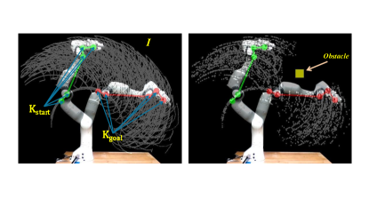
Figure 2: The images depict a vision-based motion planning problem. The left image shows the discretized representation of $I$ highlighted in gray, where each configuration is sampled as an image frame, resulting in a finite set of $\mathbb{K}$. The gray region in the right image highlights the same discretized representation of $I_{\text{free}}$, avoiding the obstacle in yellow. $I_{\text{free}}$ ensures a collision-free path from the start configuration $\mathbb{K}_{\text{start}}$ to the goal configuration $\mathbb{K}_{\text{goal}}$

III-A Model-based Motion Planning

Let $x\in\mathcal{X}$ denote the state and state-space, and $u\in\mathcal{U}$ the control and control-space of a robot system [21]. The system dynamics equations $f$ of the robot system can be written as

$$x(\mathcal{T})=x(0)+\int_{0}^{\mathcal{T}}f(x(t),u(t))dt$$ (1)

If the system dynamics impose constraints on the allowable paths the system is called a non-holonomic system. Now, Let $\mathcal{X}_{\text{obs}}\subset\mathcal{X}$ denote the invalid state space, which is the set of states that violates the robots kinematic constraints or collides with the workspace $\mathcal{W}\subseteq\mathbb{R}^{3}$. e.g.,

$$\mathcal{X}_{\text{obs}}=\{x\in\mathcal{X}|R(x)\bigcap\mathcal{W}\neq\emptyset\}$$ (2)

where $R(x)\subseteq\mathbb{R}^{3}$ is the set of all the points of the robot in the workspace at state x. Then let, $\mathcal{X}_{\text{free}}=\mathcal{X}\setminus\mathcal{X}_{\text{obs}}$ denote the collision free state-space. Also, let $x_{\text{start}}\in\mathcal{X}_{\text{free}}$ and $X_{\text{goal}}\subseteq\mathcal{X}_{\text{free}}$ denote the start state and goal regions respectively.

Motion Planning Problem: Given the motion planning tuple $(\mathcal{X},R,\mathcal{W},\mathcal{U},f,x_{\text{start}},\mathcal{X}_{G})$ find a time $\mathcal{T}$ and a set of controls $u:[0,\mathcal{T}]\rightarrow\mathcal{U}$ such that the motion described by Eq. 1 satisfies $x(0)=x_{\text{start}}$, $x(\mathcal{T})\in\mathcal{X}_{G}$ and $x(t)\in\mathcal{X}_{\text{free}}$.

III-B Vision-Only Motion Planning

The problem we are considering in this setting is departing from the above motion planning problem as the geometric model $R(x)$, the dynamics $f$ and the workspace $\mathcal{W}$ is not directly available. Instead the only information available is the space of admissible controls $\mathcal{U}$ and an image $Im\in\mathcal{IM}$.

We will describe the new problem statement by explicitly defining equivalent concepts of obstacles, robot states, and state dynamics directly in the image space. We assume that we are given a point tracking function that maps a given image to $N$ fixed pixel points on the robot’s body. This vector of pixel points is denoted as an image state $\mathbb{K}\in I$. Where $I\subset\mathbb{R}^{N\times 2}$ denotes the space of all image states. In Fig. 1 we can see $4$ different robot configurations in image space. Each configuration is represented by a set of $5$ same-colored circles. Each of these circles on the robot’s body in the image is a pixel point and is denoted as a keypoint or $\mathds{k}$. The kinematic chain or shape formed by the vector of $5$ circles represents one image state $\mathbb{K}$.

Given a set of image obstacles $\mathcal{IO}\subset Im$ we define:

$$I_{\text{obs}}=\{\mathbb{K}\in I|RI(\mathbb{K})\bigcap\mathcal{IO}\neq\emptyset\}$$ (3)

where $RI(\mathbb{K})\subseteq Im$ is the set of pixels that the robot occupies at image state $\mathbb{K}$. Similarly to before, we define $I_{\text{free}}=I\setminus I_{\text{obs}}$, $\mathbb{K}_{\text{start}}$ and $I_{g}$.

We define the unknown system dynamics function as:

$$\mathbb{K}(\mathcal{T})=\mathbb{K}(0)+\int_{0}^{\mathcal{T}}g(\mathbb{K}(t),u(t))dt$$ (4)

Here we note that even if the underlying function f is fully-integrable (holonomic-system) if $dim(I)>dim(\mathcal{X})$ the equivalent system dynamics equations $g$ will be non-holonomic as there will be paths in the higher dimensional image-space $I$ that cannot be followed by the robot. In our approach we consider this issue, and propose a way to produce paths that approximately satisfy these constraints. In the first image of Fig. 2, the grey region illustrates the discretized representation of $I$, as each configuration is captured as an image frame, resulting in a finite set of $\mathbb{K}$ sampled at a specific frame rate. The second image of Fig. 2 highlights similar discretized representation of $I_{\text{free}}$.

Given the above definitions, let us define the vision-only motion planning problem.

Vision-Only Motion Planning Problem: Given the tuple $(I,RI,\mathcal{U},\mathcal{IO},Im,\mathbb{K}_{\text{start}},I_{g})$ find a time $\mathcal{T}$ and a set of controls $u:[0,\mathcal{T}]\rightarrow\mathcal{U}$ such that the motion described by $g$ satisfies $\mathbb{K}(0)=\mathbb{K}_{\text{start}}$, $\mathbb{K}(\mathcal{T})\in I_{g}$ and $\mathbb{K}(t)\in I_{\text{free}}$.

IV Methodology

Since the system dynamics equation is unknown, we cannot directly plan in the control space $\mathcal{U}$. Instead, we will plan a path $\mathbb{K}_{0},\mathbb{K}_{1}\ldots,\mathbb{K}_{n}$ directly in the $I$-space and then control the robot to follow the path with a vision-only controller[15].

To compute the path, which is the main contribution of this work, we propose to use probabilistic road-map planner (prm) by adapting its subroutines to operate directly in $I$-space. Specifically, we opted to adapt the lazy-prm [32] planner due to its compatibility with our particular requirements. However, any sampling-based planner which relies on the the same subroutines could be used.

Algorithm 1 Build-Lazy-PRM

1:procedure Build-Lazy-PRM(N, k)

2:  $G$ $\leftarrow$ INIT()

3:  while $G$.size()$\leq$ N do

4:   $\mathbb{K}_{new}\leftarrow$ sample($I$)

5:   $G$.addNode($\mathbb{K}_{new}$)   

6:  for each $\mathbb{K}\in G$.nodes() do

7:   $\mathcal{N}(\mathbb{K})\leftarrow$ K-nearest($\mathbb{K}$, $G$)

8:   for each $\mathbb{K}_{near}\in\mathcal{N}(\mathbb{K}_{new})$ do

9:     $e\leftarrow$ ($\mathbb{K},\mathbb{K}_{near})$

10:     if $e\notin G$.edges() then

11:      $G$.addEdge($e$)           

12:  return $G$

Similar to prm, lazy-prm operates in two distinct phases, the building-phase Alg. 1 and the query-phase Alg. 2. In the building-phase, a roadmap is built without performing any collision checking. In the query-phase, the roadmap is utilized to find a potential path for a given start and goal. The key difference between lazy-prm and prm lies in their approach to collision checking. While prm verifies the collision status of all edges in the roadmap during the building phase, lazy-prm reverses the order. It first performs the search query and only checks collisions for the found path. If any edges are found to be in collision, the roadmap is updated, and another search query is executed until a valid path is discovered.

We selected probabilistic roadmap method for its efficiency in multi-query scenarios, where a single precomputed graph can handle multiple start and goal configurations, and used the lazy version, as we only have very few varying obstacles between queries. Additionally, its ability to operate in high-dimensional spaces makes it particularly well-suited for handling non-traditional representations of configuration space, such as the visual keypoints in $I$-space used in our approach. We first describe how lazy-prm works and then we describe how we modified the necessary subroutines to make it work in $I$-space.

The building-phase (Alg. 1) works with the following procedure. First, in line 4, a sample is generated and added in graph $G$. Then the k nearest nearest neighbors are found by using a distance defined in $I$ (line 7) and are connected with edges. This continues until $N$ nodes are in the graph $G$.

Algorithm 2 Query-Lazy-PRM

1:procedure Lazy-Query-PRM($\mathbb{K}_{\text{start}}$, $\mathbb{K}_{\text{goal}}$, $G$)

2:  G.add($\mathbb{K}_{\text{start}}$) $\triangleright$ Add start, and goal to the Graph

3:  G.add($\mathbb{K}_{\text{goal}}$)

4:  Edges, $\leftarrow$ Search-Graph $G$($\mathbb{K}_{\text{goal}}$, $\mathbb{K}_{\text{start}}$)

5:  for each $e\in G$.edges() do

6:   if coll_free($e$) then

7:     for each $\mathbb{K}_{near}\in\mathcal{N}(x_{new})$ do

8:      $e\leftarrow$ ($\mathbb{K},\mathbb{K}_{near})$

9:      if coll_free($e$) and $e\notin G$.edges() then

10:        $G$.addEdge($e$)            

11:     return $Path$      

During the query-phase (Alg. 2 a new motion planning problem is solved. Given a $\mathbb{K}_{\text{start}}$ and $\mathbb{K}_{\text{goal}}$ they are added in the graph, and connected with their nearest-neighbors. Then a graph search algorithm e.g., A* is used to find a path. If edges of the path are in-collision they are updated accordingly in the roadmap, and the process repeats until a collision free-path is found. The three operations sample, k-nearest, coll_free, for Alg. 1 in lines 4, 7 and Alg. 2 typically require a model for the robot.

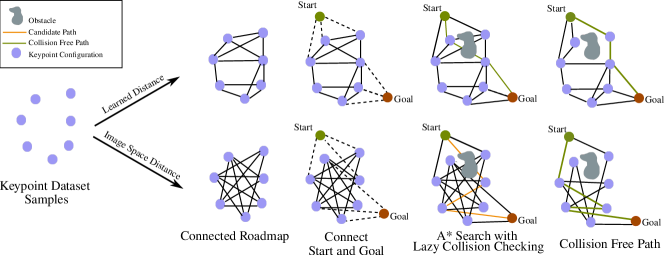
Figure 3: Overview of the roadmap creation process for motion planning. In this image the purple circles are nodes in image space represented by image state in each frame. Using a distance metric, we connect the nodes to create a roadmap. As observed two different metrics produce different edges on the graph. After an A* search for path finding between a pair of start ($\mathbb{K}_{\text{start}}$) and goal ($\mathbb{K}_{\text{goal}}$) configurations and collision check if required, paths are found for both roadmaps. The green lines denote the final path after collision check. As observed, the learned distance roadmap has a clearly more optimized path than the image space distance roadmap

sample: This function typically samples the configuration space uniformly. However, in the vision-only setting, we can’t directly sample in $I$-space as we don’t have the model of the robot. Since $dim(I)>dim(\mathcal{X})$ the keypoint vectors (image state $\mathbb{K}$) that correspond to actual configurations of the robot, will lie in a lower-dimensional (equal to $dim(\mathcal{X})$) manifold in $I$-space. Thus randomly sampling $I$-space will have $0$ probability of sampling a valid configuration that lies on the valid manifold [22]. We describe how to address this issues in subsection IV-A, by collecting and storing valid samples directly from the real robot.

k-nearest: This function usually relies on a distance defined in $\mathcal{X}$ and finds the nearest configurations that can be connected. However, since our representation in $I$-space is now a non-holonomic system, defining this distance is very challenging, as a straight line path in $I$-space defined by a simple Euclidean distance, might not be accurately followable by a controller. To mitigate this, we describe a learning-based approach to estimate the unknown joint-distance, in subsection IV-B.

coll_free: This function checks if there is a collision for an edge in $\mathcal{X}$. Again this typically requires the model $R(x)$ for the robot. In the vision only case, we propose simple yet successful method to do collision checking with an $RI(x)$ directly in $I$-space subsection IV-C.

In the next section we describe our proposed method, for each, of the aforementioned subroutines. Fig. 3 visually describes all the steps of the visual motion planning framework.

IV-A sample: Executed Trajectories as Proxy Samples

In the absence of a robot model, we represent each image state $\mathbb{K}\in I$ by identifying and annotating keypoints ($\mathds{k}$) on the robotic arm using an automated data collection pipeline described in [16, 17]. Each $\mathbb{K}_{n}$ is composed of a set of $N$ keypoints $\mathds{k}$, where each $\mathds{k}$ represents a pixel point of a specific location on the robot’s body in image space. For instance, if $N=5$, a keypoint vector or image state $\mathbb{K}_{n}$ is represented by a vector of $\mathds{k}_{1}$, $\mathds{k}_{2}$, $\mathds{k}_{3}$, $\mathds{k}_{4}$, $\mathds{k}_{5}$, where each $\mathds{k}$ is a pixel point in the $n\textsuperscript{th}$ image frame. An example vector of such keypoints is shown in Fig. 2 as $\mathbb{K}_{\text{start}}$ or $\mathbb{K}_{\text{goal}}$

To systematically explore the robot’s visible workspace in the image space and ensure comprehensive coverage, we compute velocities for each joint $j$ using:

$$v_{j}=\min\left(\frac{M_{j}}{res\cdot t},v_{\text{max}}\right),$$ (5)

where, $M_{j}$ is the motion range or difference of limits of joint $j$, $res$, is the number of discrete steps used to traverse $M_{j}$, $t$ is the duration allocated to complete each step, and $v_{\text{max}}$ is the maximum allowable velocity for joint $j$. By dividing the motion range of each joint into uniform increments based on $res$, we ensure that the robot systematically explores all possible configurations within its workspace. The resulting dataset of image states $\mathbb{K}$ is thus evenly distributed across the image space $I$, enabling robust coverage and accurate representation of the robot’s motion capabilities.

Each configuration $\mathbb{K}_{n}$ is computed using the following transformation:

$$\mathbb{K}_{n}=K\cdot T_{cw}\cdot x_{n}$$ (6)

where $K$ is the camera intrinsic matrix, $T_{cw}$ is the camera extrinsics matrix derived from calibration processes described in [33, 34], and $x_{n}$ is the 3D configuration robot in workspace. This transformation projects the 3D configuration $x_{n}$, into their corresponding 2D (pixel) projection in the image described in [35], resulting in a set of $\mathds{k}$ for each image state $\mathbb{K}_{n}$ The process captures the robot’s motion across its visible workspace and creates a comprehensive dataset of $\mathbb{K}$, representing close to all feasible configurations in image space. Dataset of $\mathbb{K}$ can also be collected by following the process describe in [17].

The Keypoint Dataset Samples section of Fig. 3, represents this part of the workflow. The grey area in the left image of Fig. 2 illustrates how $\mathbb{K}$ are distributed within image space with each frame consisting of a set of $\mathds{k}$ or keypoints. This collection process yields a large dataset of $\mathbb{K}$ that can be used to enable efficient roadmap construction for vision-based motion planning.

IV-B k-nearest: Learned and Image-Space Metrics

To search for the K-nearest neighbors of each image state sample we employ the following two distance metrics:

• Learned distance, where the distance is learned by a neural network, trained to predict joint displacements between two image states. The input to the network is a pair of image states $\mathbb{K}_{1}$ and $\mathbb{K}_{2}$ and and the output is an estimated joint displacement required to transition between them:

  $$\text{dist}_{learned}()\leftarrow\text{NN}(\mathbb{K}_{1},\mathbb{K}_{2})$$ (7)

• Distance in Image space, where we simply calculate the Euclidean distance between $\mathbb{K}_{1}$ and $\mathbb{K}_{2}$ in image space:

  $$\text{dist}_{image}()\leftarrow||\mathbb{K}_{1}-\mathbb{K}_{2}||_{2}$$ (8)

Each metric influences the graph’s structure by determining the nearest neighbors and defining the edges in the roadmap. The learned distance prioritizes image states with minimal estimated joint displacement, while the image space distance favors image states that are closer in the image. These differences impact the connectivity of the roadmap, as illustrated in the Connected Roadmap and Connect Start and Goal sections of Fig. 3.

IV-B1 Dataset generation for network model

While collecting the dataset of image states $\mathbb{K}$ in subsection IV-A, we recorded the velocity (Eq. 5) applied to transition between consecutive frames. Using this data, we created a new dataset that includes pairs of consecutive image states ($\mathbb{K}_{1}$, $\mathbb{K}_{2}$) and their estimated joint displacements. This is calculated by multiplying the recorded velocity with the frame rate at which $\mathbb{K}$ was captured, as described in Eq. 6.

Please note here, only pairs of $\mathbb{K}$ captured in consecutive image frames are included in this data generation process. However, for constructing the graph $G$, it is essential to compute distances between arbitrary $\mathbb{K}$ pairs in $I$-space. To achieve this, a neural network is employed to predict the joint displacement across different pairs of image-states $\mathbb{K}$.

To enhance diversity, the dataset is augmented by combining frame sequences where the first frame’s image state ($\mathbb{K}_{\text{start}}$) and the last frame’s image state ($\mathbb{K}_{\text{end}}$) act as boundaries, with total joint displacements calculated as sum of displacements across intermediate frames. This approach ensures diverse transitions, enabling the neural network to accurately estimate joint displacements for any image state pair.

IV-B2 Neural Network for Learned Distance Metric

To derive Eq. 7, we design a simple neural network using the aforementioned dataset to learn a distance more similar to the joint space distance. The model takes concatenated arrays of the starting image state ($\mathbb{K}_{\text{start}}$) and the subsequent image state ($\mathbb{K}_{\text{next}}$) as input and predicts the estimated joint displacement.

IV-C coll_free:Image-Based Collision Checking

To check for collisions in our model-free system, we employ an image-based polygon collision-checking framework. Polygons are formed by connecting pairs of consecutive keypoints (($\mathds{k}_{n-1}$), ($\mathds{k}_{n}$)) in one image state ($\mathbb{K}_{1}$) with their corresponding keypoints in the neighboring image state ($\mathbb{K}_{2}$). In Fig. 4, the polygons created by ($\mathds{k}_{1}$, $\mathds{k}_{2}$), ($\mathds{k}_{2}$, $\mathds{k}_{3}$), ($\mathds{k}_{3}$, $\mathds{k}_{4}$) and ($\mathds{k}_{4}$, $\mathds{k}_{5}$) of the start image state ($\mathbb{K}_{1}$) in green and its neighboring image state ($\mathbb{K}_{2}$) in red are examples of such polygons.

Each polygon is then checked for intersections with the obstacle boundaries defined by a safety margin which we consider to account for controller uncertainty. This polygon-based approach ensures a thorough and robust collision-checking process, effectively handling obstacles of any size. In Fig. 4 illustrates an example where the obstacle, enclosed by the red safety margin, intersects with the polygons defined by ([$\mathds{k}_{2}$, $\mathds{k}_{3}$],[$\mathds{k}_{3}$, $\mathds{k}_{4}$] and [$\mathds{k}_{4}$, $\mathds{k}_{5}$]), demonstrating the effectiveness of this method. The collision checking process and A* search is shown in A* Search with Lazy Collision Checking of Fig. 3.

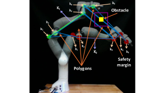
Figure 4: Illustration of polygon-based collision checking for vision-only motion planning. In this image $4$ polygons (bordered with light blue) are defined by connecting consecutive keypoint pairs ($\mathds{k}_{1}$, $\mathds{k}_{2}$), ($\mathds{k}_{2}$, $\mathds{k}_{3}$), ($\mathds{k}_{3}$, $\mathds{k}_{4}$) and ($\mathds{k}_{4}$, $\mathds{k}_{5}$) of the image state ($\mathbb{K}_{1}$) in green and its neighboring image state ($\mathbb{K}_{2}$) in red. The yellow obstacle enclosed by the purple safety margin is situated right on the polygons formed by ([$\mathds{k}_{2}$, $\mathds{k}_{3}$],[$\mathds{k}_{3}$, $\mathds{k}_{4}$] and [$\mathds{k}_{4}$, $\mathds{k}_{5}$]), rendering these two configurations ineligible for a collision-free path.

IV-D Adaptive Visual Servoing

This work builds on the adaptive visual servoing method described in [15], using a roadmap of collision-free sequence of goal image states. At each goal, vector of keypoints ($\mathds{k}$) in image state ($\mathbb{K}$), is tracked as visual features as described in [16]. The controller moves the arm minimizing the feature error, computed as the difference between the current and the target $\mathbb{K}$. The Jacobian matrix, estimated online via least-square optimization of recent joint velocities and keypoints vector over a moving window, eliminates the need to read joint position from encoder. This makes the control pipeline completely model-free. To improve accuracy, we reset the Jacobian estimation window at each new target keeping the estimate unbiased and relevant to the current goal. Since the goals may not be evenly spaced in the image for different experiments, we use a saturation limit on the feature error to prevent sudden spikes in velocity ensuring stable motion and protecting the motor from damage.

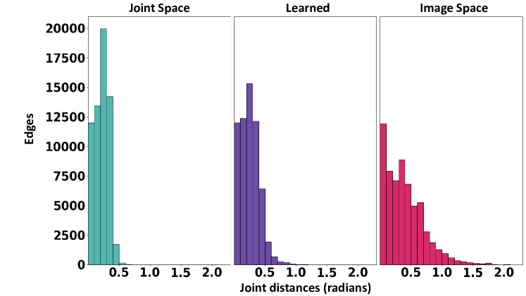
Figure 5: Histograms of actual joint displacements along the edges for the three roadmaps. The Learned roadmap closely aligns with the distribution of the Joint Space roadmap, showing only slight deviations and indicating reasonable accuracy in the predicted joint displacements. In contrast, the Image space roadmap demonstrates a wider spread and larger joint displacements, reflecting its lack of alignment between image-space proximity and joint-space movements. This misalignment may reduce its efficiency in generating paths suitable for precise control.

V Experiments and Observations:

We experimentally assesed the performance of the proposed vision only motion planning framework on a Franka Emika Panda Arm.

V-A Experimental details

V-A1 Generating samples

We generated the required image state samples by collecting a large dataset created by actuating the planar joints (Joints $2,4,6$) of the Franka arm, using velocities computed from Eq. 5 as explained in subsection IV-A, covering the robot’s planar workspace.

V-A2 Generating the roadmap

The collected samples $\mathbb{K}$ were used as nodes to generate roadmaps using the different proposed distances described in subsection IV-B. The roadmap generated by the image-space distance is coined as Image Space roadmap and the one generated using the learned distance is coined as Learned roadmap. For benchmarking purposes we also use the actual joint distance to create the Joint Space roadmap. The Joint Space roadmap used actual joint displacements from encoders solely for benchmarking, maintaining the proposed model-free framework. The k-neighbor value for all approaches was set to $25$.

V-A3 Obstacle Representation and Path Planning

In the experimental setup, obstacles were modeled as virtual yellow rectangles with a safety margin, as shown in Fig. 4. Paths were generated offline for various start ($\mathbb{K}_{\text{start}}$) and goal ($\mathbb{K}_{\text{goal}}$) incorporating the obstacle avoidance logic from subsection IV-C. These paths were later used in adaptive visual servoing experiments

V-A4 Control Experiment Set-up

The real-time control experiments used an Intel Realsense D435i camera in an eye-to-hand setup for visual feedback. The Panda arm followed the planned paths in $16$ obstacle-free and $10$ obstacle-avoidance experiments. The performance of each proposed roadmap was evaluated by comparing the joint position changes between intermediate image states to those of the Joint Space roadmap. The controller’s ability to guide the arm along collision-free paths was evaluated for efficiency and effectiveness.

V-B Roadmap and Path Planning Experiments

In this section, we analyze the joint displacements along the edges of the three roadmaps to evaluate their efficiency. Path planning experiments were conducted in both collision-free and obstacle-avoidance scenarios to compare the joint distances covered by the paths generated from each roadmap.

V-B1 Distribution of Joint Distances of Edges for Different Roadmaps

Fig. 5 shows the histograms of joint displacements along the edges of the three roadmaps. The Learned roadmap closely aligns with the joint space roadmap with minor deviations, demonstrating reasonable accuracy in estimated joint displacements. In contrast, the Image Space roadmap exhibits a broader spread and larger joint displacements. This suggests that the Learned roadmap is more effective in accurately capturing transitions and generating paths that minimize joint movements.

V-B2 Average Joint Distances for Planned Collision-Free Paths

We randomly selected $100$ pairs of $\mathbb{K}_{\text{start}}$ and $\mathbb{K}_{\text{goal}}$ from the roadmaps for path planning without obstacles. The average joint distances over $100$ trials, summarized in subsubsection V-B2, show that the learned roadmap yields results closer to the joint space while the image space roadmap results in significantly larger joint displacements. These findings suggest that the learned roadmap possibly generates more efficient path, better suited for successful control convergence.

TABLE I: Average Joint Distances (Radians) for Collision-Free Paths

	Joint Space	Learned	Image
Space
Mean
(radians)	1.74	2.19	3.06

V-B3 Planned paths for Control Experiments

We generated planned paths for two scenarios: $16$ start and goal pairs without checking for collision and $10$ pairs with collision avoidance. Paths were computed using the three roadmaps: Joint Space, Learned, and Image Space. These precomputed paths were used in the control experiments described in subsection V-C.

For each planned path, we calculated metrics including the average number of waypoints (intermediate image states), joint distances between waypoints, total joint distances for the entire path, and Euclidean distances between image states (keypoint distances) both between waypoints and across the entire path.

As observed in Table II the learned roadmap consistently resulted in fewer waypoints and shorter joint distances compared to the image space roadmap, which prioritizes minimizing keypoints distances in image space but incurs higher joint displacements.

Notably, the joint distances required to traverse $1000$ pixels in image space were much higher for the Image space roadmap than for the Learned roadmap. This suggests that reliance on image space proximity may lead to less efficient joint-space paths.

TABLE II: Comparison of Joint Distances and Keypoints Distance in Image Space over Experiments

	Without Collision-check			With Collision-check
Roadmaps	Joint Space	Learned	Image Space	Joint Space	Learned	Image Space
Number of Experiments	16	16	16	10	10	10
Avg No. of Waypoints	8	8	14	11	13	15
Avg. Joint Distances (radians) b/w Waypoints	0.25	0.3	0.32	0.28	0.28	0.35
Avg. Keypoints Distances (pixels) b/w Waypoints	167.99	174.76	84.11	139.53	129.13	89.36
Avg. Joint Distances (radians) over Entire Path	1.92	2.27	4.29	3.04	3.46	5.36
Avg. Keypoints Distances (pixels) over Entire Path	1222.42	1278.92	1157.00	1532.72	1569.37	1361.43
Joint Distance (radians) Traversed To Move 1000 pixels in image space	1.6	1.77	3.79	1.98	2.19	3.9

We have two theories from the above observations:

• The larger number of waypoints in the image space roadmap arises from its Euclidean distance-based edge weights, causing A* to prioritize shorter pixel distances and select more intermediate nodes. In contrast, the learned roadmap, with joint displacement-based weights, produces more direct paths with fewer waypoints.

• The image states $\mathbb{K}$ which are close in image space may be much further away in joint space as highlighted in Table II. This behavior may lead to increased overall joint movement where non-holonomy may exist in the joint space for the covered joint displacements. This may reduce control accuracy and hinder convergence to the target image state.

V-C Control Experiments

The adaptive visual servoing experiments used precomputed paths from subsubsection V-B3, with control gains optimized to minimize rise and settling times while keeping overshoot within 5%, by careful tuning.

In subsection V-C, the overall control metrics highlight that the image space roadmap succeeded in only $69.2$% of cases, while the learned roadmap achieved a $100$% success rate. However, the image space roadmap, when successful, showed faster transient responses compared to the Learned roadmap. Table IV uses identical metrics as in Table II, categorizing experiments into successful and failed cases

Failures in the image space roadmap were characterized by large joint displacements relative to smaller image space distances, as noted earlier in subsubsection V-B3. Optimal execution of the references generated by using image space distances requires all the keypoints to follow straight paths. This is not possible for the robot due to the non-holonomic constraints of its kinematics (if defined directly in image space). As a result, the robot deviates from the planned path. While the robot reaches the reference locations in most cases, the deviations cause it to go out of its workspace (due to joint limits) in some others. This effect is especially visible when obstacles exist in the workspace since the robot needs to travel near the edges of its workspace to avoid them. When estimated joint distances are used the resulting trajectories are more suitable to the robot’s kinematics, which prevents such failures at large.

TABLE III: Performance results for the control experiments with and without obstacle

	Without Collision-check			With Collision-check
Performance
Metrics	Joint
Space	Learned	Image
Space	Joint
Space	Learned	Image
Space
Successful
Experiments	16/16	16/16	13/16	10/10	10/10	5/10
System
Rise time (s)	74.92	97.53	94.75	105.38	125.38	90.46
System
Settling time (s)	94.37	118.62	101.99	118.18	155.14	96.44
End effector
Rise time (s)	74.86	97.53	94.39	105.02	125.38	90.46
End effector
Settling time (s)	94.37	114.02	99.81	118.18	147.14	94.22
Overshoot (%)	1.94	2.61	1.89	1.93	2.36	1.35
Execution
time (s)	125.17	148.92	140.78	146.02	201.68	124.70

TABLE IV: Comparison of Joint Distances and Keypoints Distance in Image Space over Experiments for Successful and Failed Experiments

	Successful			Failed (Image Space)
Roadmaps	Joint Space	Learned	Image Space	Joint Space	Learned	Image Space
Number of Experiments	18	18	18	8	8	8
Avg No. of Waypoints	8	8	14	11	13	15
Avg. Joint Distances (radians) b/w Waypoints	0.25	0.3	0.32	0.27	0.29	0.35
Avg. Keypoints Distances (pixels) b/w Waypoints	166.77	163.41	86.03	135.17	143.24	86.35
Avg. Joint Distances (radians) over Entire Path	2.10	2.37	4.42	2.92	3.52	5.33
Avg. Keypoints Distances (pixels) over Entire Path	1307.02	1257.02	1210.93	1419.93	1691.26	1291.2
Joint Distance (radians) Traversed To Move 1000 pixels in image space	1.6	1.9	3.71	2.1	2.1	4.12

To summarize, both the image space and learned roadmaps exhibit unique benefits. The image space roadmap provides faster execution when successful but struggles in reliability and path convergence. The learned roadmap, using joint displacement-based distances, avoids non-holonomic constraints and ensures robustness, particularly in complex paths. The choice between the two ultimately depends on the specific application context.

VI Conclusion and Future Work

In conclusion, this work introduced a novel framework for collision-free motion planning of robotic manipulators that relied solely on visual features, eliminating the need for explicit robot models or encoder feedback.

The learned roadmap offered smoother, more reliable transitions, and due to its joint displacement-based distance definition, the paths it generated maintained joint-space holonomy when it existed. In contrast, the paths produced by the image space roadmap sometimes failed to maintain joint-space holonomy, even when holonomy existed in the image space. However, the image space roadmap provided faster transient responses and simplicity, making it advantageous for applications where speed and computational efficiency were prioritized.

Future work will explore extending this approach to out-of-plane motion and incorporating real-world obstacles to develop a fully integrated control and manipulation pipeline.

References

- [1] S. Hutchinson, G. D. Hager, and P. I. Corke, “A tutorial on visual servo control,” IEEE Trans. Robot., vol. 12, no. 5, pp. 651–670, 1996.
- [2] K. Hashimoto, “A review on vision-based control of robot manipulators,” Adv. Robot., vol. 17, no. 10, pp. 969–991, 2003.
- [3] B. Calli and A. M. Dollar, “Vision-based precision manipulation with underactuated hands: Simple and effective solutions for dexterity,” in IEEE/RSJ Intl. Conf. on Intell. Robots and Syst., vol. Nov, 2016, pp. 1012–1018.
- [4] H. Cuevas-Velasquez, N. Li, R. Tylecek, M. Saval-Calvo, and R. B. Fisher, “Hybrid multi-camera visual servoing to moving target,” in IEEE/RSJ Intl. Conf. on Intell. Robots and Syst., 2018, pp. 1132–1137.
- [5] P. Ardón, M. Dragone, and M. S. Erden, “Reaching and grasping of objects by humanoid robots through visual servoing,” in Haptics: Science, Technology, and Applications: 11th Intl. Conf., EuroHaptics, Proceedings, Part II 11. Springer, 2018, pp. 353–365.
- [6] J. Lai, K. Huang, B. Lu, and H. K. Chu, “Toward vision-based adaptive configuring of a bidirectional two-segment soft continuum manipulator,” IEEE/ASME Intl. Conf. on Adv. Intell. Mechatronics, AIM, vol. July, pp. 934–939, 2020.
- [7] M. Luo, R. Yan, Z. Wan, Y. Qin, J. Santoso, E. H. Skorina, and C. D. Onal, “Orisnake: Design, fabrication, and experimental analysis of a 3-d origami snake robot,” IEEE Robot. Autom. Letters, vol. 3, no. 3, pp. 1993–1999, 2018.
- [8] P. Liu, M. N. Huda, L. Sun, and H. Yu, “A survey on underactuated robotic systems: bio-inspiration, trajectory planning and control,” Mechatronics, vol. 72, p. 102443, 2020.
- [9] A. Gandhi, S.-S. Chiang, C. D. Onal, and B. Calli, “Shape control of variable length continuum robots using clothoid-based visual servoing,” in IEEE/RSJ Intl. Conf. on Intell. Robots and Syst., 2023, pp. 6379–6386.
- [10] I. Chavdarov, V. Nikolov, B. Naydenov, and G. Boiadjiev, “Design and control of an educational redundant 3d printed robot,” in IEEE Intl. Conf. on Software, Telecommunications and Computer Networks, 2019, pp. 1–6.
- [11] C. D. Onal, M. T. Tolley, R. J. Wood, and D. Rus, “Origami-inspired printed robots,” IEEE/ASME Trans. on Mechatronics, vol. 20, no. 5, pp. 2214–2221, 2014.
- [12] M. A. M. Adzeman, M. H. M. Zaman, M. F. Nasir, M. Faisal, and S. M. M. Ibrahim, “Kinematic modeling of a low cost 4 dof robot arm system,” Intl. J. of Emerging Trends in Engineering Research, vol. 8, no. 10, 2020.
- [13] H. Wang, B. Yang, J. Wang, X. Liang, W. Chen, and Y.-H. Liu, “Adaptive visual servoing of contour features,” IEEE/ASME Trans. on Mechatronics, vol. 23, no. 2, pp. 811–822, 2018.
- [14] D. Navarro-Alarcon and Y.-H. Liu, “Fourier-based shape servoing: A new feedback method to actively deform soft objects into desired 2-d image contours,” IEEE Trans. Robot., vol. 34, no. 1, pp. 272–279, 2017.
- [15] A. Gandhi, S. Chatterjee, and B. Calli, “Skeleton-based adaptive visual servoing for control of robotic manipulators in configuration space,” in IEEE/RSJ Intl. Conf. on Intell. Robots and Syst., 2022, pp. 2182–2189.
- [16] S. Chatterjee, A. C. Karade, A. Gandhi, and B. Calli, “Keypoints-based adaptive visual servoing for control of robotic manipulators in configuration space,” in IEEE/RSJ Intl. Conf. on Intell. Robots and Syst., 2023, pp. 6387–6394.
- [17] S. Chatterjee, D. Doan, and B. Calli, “Utilizing inpainting for training keypoint detection algorithms towards markerless visual servoing,” in IEEE Intl. Conf. Robot. Autom., 2024, pp. 3086–3092.
- [18] L. E. Kavraki, P. Svestka, J.-C. Latombe, and M. H. Overmars, “Probabilistic roadmaps for path planning in high-dimensional configuration spaces,” IEEE Trans. Robot., vol. 12, no. 4, pp. 566–580, 1996.
- [19] J. Schulman, Y. Duan, J. Ho, A. Lee, I. Awwal, H. Bradlow, J. Pan, S. Patil, K. Goldberg, and P. Abbeel, “Motion planning with sequential convex optimization and convex collision checking,” Intl. J. of Robotics Research, vol. 33, no. 9, pp. 1251–1270, 2014.
- [20] Z. Zhao, S. Cheng, Y. Ding, Z. Zhou, S. Zhang, D. Xu, and Y. Zhao, “A survey of optimization-based task and motion planning: from classical to learning approaches,” IEEE/ASME Trans. on Mechatronics, 2024.
- [21] A. Orthey, C. Chamzas, and L. E. Kavraki, “Sampling-based motion planning: A comparative review,” Annual Review of Control, Robot., and Autom. Syst., vol. 7, no. 1, 2024.
- [22] Z. Kingston, M. Moll, and L. E. Kavraki, “Sampling-based methods for motion planning with constraints,” Annual Review of Control, Robot., and Autom. Syst., vol. 1, no. 1, pp. 159–185, 2018.
- [23] M. Likhachev, G. J. Gordon, and S. Thrun, “Ara*: Anytime a* with provable bounds on sub-optimality,” Advances in Neural Information Processing Systems, vol. 16, 2003.
- [24] B. J. Cohen, S. Chitta, and M. Likhachev, “Search-based planning for manipulation with motion primitives,” in IEEE Intl. Conf. Robot. Autom., 2010, pp. 2902–2908.
- [25] S.-O. Park, M. C. Lee, and J. Kim, “Trajectory planning with collision avoidance for redundant robots using jacobian and artificial potential field-based real-time inverse kinematics,” Intl. J. on Control, Autom. and Syst., vol. 18, no. 8, pp. 2095–2107, 2020.
- [26] W. Liu, H. Niu, M. N. Mahyuddin, G. Herrmann, and J. Carrasco, “A model-free deep reinforcement learning approach for robotic manipulators path planning,” in IEEE Intl. Conf. on Control, Autom. and Syst., 2021, pp. 512–517.
- [27] D. Zhou, R. Jia, H. Yao, and M. Xie, “Robotic arm motion planning based on residual reinforcement learning,” in IEEE Intl. Conf. on Computer and Autom. Engineering, 2021, pp. 89–94.
- [28] B. Ichter and M. Pavone, “Robot motion planning in learned latent spaces,” IEEE Robot. Autom. Letters, vol. 4, no. 3, pp. 2407–2414, 2019.
- [29] M. Zeller, R. Sharma, and K. Schulten, “Vision-based motion planning of a pneumatic robot using a topology representing neural network,” in IEEE Intl. Symp. on Intell. Control, 1996, pp. 7–12.
- [30] Y. Mezouar and F. Chaumette, “Path planning in image space for robust visual servoing,” in IEEE Intl. Conf. Robot. Autom., vol. 3, 2000, pp. 2759–2764.
- [31] D. Lee, H. Lim, and H. J. Kim, “Obstacle avoidance using image-based visual servoing integrated with nonlinear model predictive control,” in IEEE Conf. on Decision and Control and European Control Conference, 2011, pp. 5689–5694.
- [32] R. Bohlin and L. E. Kavraki, “Path planning using lazy prm,” in IEEE Intl. Conf. Robot. Autom., vol. 1, 2000, pp. 521–528.
- [33] T. E. Lee, J. Tremblay, T. To, J. Cheng, T. Mosier, O. Kroemer, D. Fox, and S. Birchfield, “Camera-to-robot pose estimation from a single image,” in IEEE Intl. Conf. Robot. Autom., 2020, pp. 9426–9432.
- [34] Z. Zhang, “A flexible new technique for camera calibration,” IEEE Trans. on Pattern Analysis and Machine Intelligence, vol. 22, pp. 1330–1334, 2000.
- [35] Camera calibration and 3d reconstruction. [Online]. Available: https://docs.opencv.org/4.x/d9/d0c/group˙˙calib3d.html