Computation of Magnetohydrodynamic Equilibria with Voigt Regularization

Abstract

This work presents the first numerical investigation of using Voigt regularization as a method for obtaining magnetohydrodynamic (MHD) equilibria without the assumption of nested magnetic flux surfaces. Voigt regularization modifies the MHD dynamics by introducing additional terms that vanish in the infinite-time limit, allowing for magnetic reconnection and the formation of magnetic islands, which can overlap and produce field-line chaos. The utility of this approach is demonstrated through numerical solutions of two-dimensional ideal and resistive test problems. Our results show that Voigt regularization can significantly accelerate the convergence to solutions in resistive MHD problems, while also highlighting challenges in applying the method to ideal MHD systems. This research opens up new possibilities for developing more efficient and robust MHD equilibrium solvers, which could contribute to the design and optimization of future fusion devices.

I Introduction

Magnetohydrodynamic (MHD) equilibrium solutions, with and without flows, have a wide range of applications in space and laboratory plasma experiments, including planetary magnetospheres, stellar atmospheres,[1] and magnetic fusion devices.[2] For magnetic confinement fusion applications, equilibria without flow (also referred to as magnetohydrostatic (MHS)) are usually a first point of departure. Furthermore, solutions with a continuum of nested flux surfaces are desirable for fusion devices. Therefore, many three-dimensional (3D) equilibrium solvers assume this as a starting point.[3, 4, 5] It is well-known, however, that ideal three-dimensional (3D) toroidal MHS equilibria with nested flux surfaces are usually ill-behaved at rational surfaces where magnetic field lines close on themselves.[6] Specifically, delta-function and algebraically diverging singularities of current density can arise at those surfaces.[7, 8] These singular current densities are integrable and do not pose a problem as far as weak solutions are concerned.[9, 10] Their presence, however, indicates that those flux surfaces in a real plasma will tear and reconnect, forming magnetic islands, which can overlap and produce chaotic field-line regions. Moreover, because rational surfaces are dense if the rotational transform $\iota$ has a continuous profile, the corresponding ideal MHS equilibrium may have densely distributed singularities throughout the entire volume. Calculating numerical approximations for such an equilibrium is a formidable challenge.

To resolve this issue of densely distributed singularities in 3D equilibria, approaches to regularize MHS equilibria have been proposed. A prominent example is the multi-region relaxed magnetohydrodynamics (MRxMHD).[11] In the MRxMHD description, the entire plasma volume is divided into multiple regions. In each region, the magnetic field relaxes to a Beltrami field (also known as a Taylor state) satisfying $\nabla\times\boldsymbol{B}=\mu\boldsymbol{B}$ while conserving magnetic helicity in that domain. The force-balance condition is enforced across the interfaces between regions. Because Beltrami fields are force-free, the plasma pressure in each region is constant. Over the entire volume, the plasma pressure comprises a sequence of step functions, with discontinuities at the interfaces between regions. To maintain force-balance across the interfaces with discontinuous pressure, the magnetic field must also be discontinuous, corresponding to delta-function singular current densities. The MRxMHD model bridges Taylor relaxation[12] and ideal MHD: When the entire volume contains only one region, MRxMHD is equivalent to Taylor relaxation, whereas in the limit of infinite number of regions, MRxMHD approaches ideal MHD under certain conditions.[13, 14] A numerical code to solve MRxMHD equilibria, the Stepped Pressure Equilibrium Code (SPEC), has been developed by Hudson et al.[15]

One of the strong attributes of MRxMHD is that it allows magnetic islands and field-line chaos within each region, but the interfaces between regions form a set of nested surfaces that cannot break. The placement of the interfaces is arbitrary and remains a critical issue of MRxMHD research.[16, 14, 17] Usually the interfaces are placed at surfaces of strongly irrational rotational transform $\iota$ (i.e., it satisfies the Diophantine condition) because those flux surfaces are more difficult to break.[18] More generally, MRxMHD also permits solutions with discontinuous rotational transform profiles.[19]

The uncertainties in the choice of interfaces can pose challenges in constructing MRxMHD solutions, motivating consideration of other approaches to regularizing the MHD equilibrium. For example, Dewar and Qu have recently proposed an augmented Lagrangian multiplier method to approximate the ideal MHD Ohm’s law.[20] This method avoids the exact enforcement of the ideal Ohm’s law constraint, which is the source of current singularities. The present study considers another approach to regularizing the MHD equilibrium using the so-called Voigt approximation. This approach is motivated by a recent mathematical theorem of Constantin and Pasqualotto.[21] The theorem claims that the infinite-time limit of the Voigt approximations of viscous, non-resistive, incompressible MHD equations are MHS equilibria that are regular and non-Beltrami. The Voigt approximation modifies MHD dynamics by introducing additional terms in the governing equations, which vanish as the solution asymptotically becomes time-independent (in the infinite-time limit).

This paper is organized as follows. Section II lays out the formalism of the Voigt-MHD equations and derives the energy conservation law and the wave dispersion relation. The Voigt approximation modifies the form of total energy, which involves current density and vorticity. This modified energy form provides critical insight into why the Voigt approximation regularizes the solution. The wave dispersion relation further suggests that the Voigt approximation slows down MHD waves, allowing larger time-steps and potentially expediting the convergence to equilibrium. Section III assesses the feasibility and effectiveness of using the Voigt approximation by numerically solving two-dimensional (2D) test problems of MHD equilibria. We first describe a 2D pseudospectral numerical solver of Voigt-MHD in slab geometry using the Dedalus framework.[22] We then apply the solver to a few ideal and resistive test problems, including the saturation of the tearing instability[16] and the Hahm–Kulsrud–Taylor forced reconnection problem.[23] These test problems have a common theme of magnetic island formation. Section IV discusses the implications of our findings, open questions, and future perspectives of applying the Voigt regularization for the development of more robust and efficient MHD equilibrium solvers.

II Voigt Regularization of Incompressible Magnetohydrodynamics

II.1 Governing Equations and Boundary Conditions

The non-dimensional form of Voigt-regularized, incompressible MHD system is given by

$$\partial_{t}\left(\boldsymbol{u}-\alpha_{1}\nabla^{2}\boldsymbol{u}\right)+\boldsymbol{u}\cdot\nabla\boldsymbol{u}=-\nabla p+\boldsymbol{J}\times\boldsymbol{B}+\nu\nabla^{2}\boldsymbol{u},$$ (1)

$$\partial_{t}\left(\boldsymbol{B}-\alpha_{2}\nabla^{2}\boldsymbol{B}\right)=\nabla\times\left(\boldsymbol{u}\times\boldsymbol{B}-\eta\boldsymbol{J}-\boldsymbol{E}_{\text{ext}}\right),$$ (2)

$$\boldsymbol{J}=\nabla\times\boldsymbol{B},$$ (3)

$$\nabla\cdot\boldsymbol{u}=\nabla\cdot\boldsymbol{B}=0.$$ (4)

Standard notations are used: $\boldsymbol{u}$ is the plasma velocity, $\boldsymbol{B}$ is the magnetic field, $p$ is the pressure, $\boldsymbol{J}$ is the current density, $\nu$ is the viscosity coefficient, and $\eta$ is the resistivity. Voigt regularization adds two terms within the time derivatives: $-\alpha_{1}\nabla^{2}\boldsymbol{u}$ and $-\alpha_{2}\nabla^{2}\boldsymbol{B}$, where the coefficients $\alpha_{1}$ and $\alpha_{2}$ are free parameters.

The induction equation (2) corresponds to a generalized Ohm’s law

$$\boldsymbol{E}=-\boldsymbol{u}\times\boldsymbol{B}+\alpha_{2}\partial_{t}\boldsymbol{J}+\eta\boldsymbol{J}+\boldsymbol{E}_{\text{ext}}.$$ (5)

When $\eta>0$ , an external electric field $\boldsymbol{E}_{\text{ext}}$ is applied to prevent the solution from decaying to a vacuum field. The term $\alpha_{2}\partial_{t}\boldsymbol{J}$ coming from Voigt regularization is analogous to the electron inertia term in a generalized Ohm’s law.[24] Similar to the electron inertia effect, the $\alpha_{2}\partial_{t}\boldsymbol{J}$ term breaks the frozen-in condition, allowing magnetic reconnection even when the resistivity vanishes.

The boundaries are assumed to be impenetrable, no-slip, and perfectly conducting, leading to the following boundary conditions:

$$\left.\boldsymbol{u}\right|_{\text{wall}}=0,$$ (6)

and

$$\left.\boldsymbol{\hat{n}}\times\boldsymbol{E}\right|_{\text{wall}}=\left.\boldsymbol{\hat{n}}\times\left[\alpha_{2}\partial_{t}\boldsymbol{J}+\eta\boldsymbol{J}+\boldsymbol{E}_{\text{ext}}\right]\right|_{\text{wall}}=0,$$ (7)

where $\boldsymbol{\hat{n}}$ is the unit normal vector to the wall.

An important feature of the Voigt regularization is that all the additional terms are within the time derivative terms of the momentum and induction equations. In the infinite-time limit when the solution approaches a steady state, those terms vanish. Therefore, the Voigt-regularization terms have no effect on the force-balance once a steady-state solution is obtained.

II.2 Energy Conservation

The energy conservation law for the Voigt-MHD system can be obtained by adding the inner product of Eq. (1) with $\boldsymbol{u}$ and the inner product of Eq. (2) with $\boldsymbol{B}$, and integrating the sum over the entire volume. We break the derivation into several parts. First, note that for an incompressible flow, the condition $\nabla^{2}\boldsymbol{u}=-\nabla\times\boldsymbol{\omega}$ is satisfied, where $\boldsymbol{\omega}=\nabla\times\boldsymbol{u}$ is the vorticity. We can then derive the equation

$$\boldsymbol{u}\cdot\nabla^{2}\boldsymbol{u}=-\boldsymbol{u}\cdot\nabla\times\boldsymbol{\omega}=\nabla\cdot\left(\boldsymbol{u}\times\boldsymbol{\omega}\right)-\omega^{2},$$ (8)

by using vector identities. Likewise, we have

$$\boldsymbol{B}\cdot\nabla^{2}\boldsymbol{B}=\nabla\cdot\left(\boldsymbol{B}\times\boldsymbol{J}\right)-J^{2}.$$ (9)

From Eqs. (8) and (9), we obtain

$$\boldsymbol{u}\cdot\partial_{t}\nabla^{2}\boldsymbol{u}=\nabla\cdot\left(\boldsymbol{u}\times\partial_{t}\boldsymbol{\omega}\right)-\partial_{t}\frac{\omega^{2}}{2},$$ (10)

and

$$\boldsymbol{B}\cdot\partial_{t}\nabla^{2}\boldsymbol{B}=\nabla\cdot\left(\boldsymbol{B}\times\partial_{t}\boldsymbol{J}\right)-\partial_{t}\frac{J^{2}}{2}.$$ (11)

Next, the identities

$$\boldsymbol{B}\cdot\nabla\times\left(\boldsymbol{u}\times\boldsymbol{B}\right)=\nabla\cdot\left(\left(\boldsymbol{u}\times\boldsymbol{B}\right)\times\boldsymbol{B}\right)-\boldsymbol{u}\cdot\left(\boldsymbol{J}\times\boldsymbol{B}\right),$$ (12)

and

$$\boldsymbol{B}\cdot\nabla\times\left(\eta\boldsymbol{J}+\boldsymbol{E}_{\text{ext}}\right)=\nabla\cdot\left(\left(\eta\boldsymbol{J}+\boldsymbol{E}_{\text{ext}}\right)\times\boldsymbol{B}\right)+J^{2}+\boldsymbol{E}_{\text{ext}}\cdot\boldsymbol{J},$$ (13)

are readily derived.

Using Eqs (8) – (13), the energy conservation law can be written as

$$\frac{d}{dt}\int d^{3}x\left(\frac{u^{2}+\alpha_{1}\omega^{2}+B^{2}+\alpha_{2}J^{2}}{2}\right)$$

$$= -\int d^{3}x\left(\nu\omega^{2}+\eta J^{2}\right)-\int d^{3}x\boldsymbol{E}_{\text{ext}}\cdot\boldsymbol{J},$$ (14)

where several surface integral terms are shown to vanish by using the boundary conditions (6) and (7). The left-hand-side of Eq. (14) is the time derivative of the “energy” in Voigt-MHD. The first term on the right-hand-side represents the energy dissipated due to viscosity and resistivity, whereas the second term accounts for the energy injected or extracted by the external electric field.

The presence of $\alpha_{1}\omega^{2}+\alpha_{2}J^{2}$ in the energy functional provides a critical insight as to why the Voigt terms regularize the solution. For the “ideal” case with $\eta=0$ and $\boldsymbol{E}_{\text{ext}}=0$, the total energy remains bounded, which precludes the formation of delta-function current density and vorticity, otherwise $J^{2}$ or $\omega^{2}$ will become non-integrable. Although energy consideration alone cannot preclude algebraically divergent current density and vorticity completely, their formation is strongly restricted by the requirement of energy being bounded. More generally, Voigt terms of the form $\alpha\nabla^{2n}$ can be considered if higher-order regularity is desired.[21]

II.3 Wave Dispersion Relation

The wave dispersion relation provides insight into the behavior of waves, which is critical for developing efficient and stable numerical methods for solving the system. We consider the dispersion relation of a plane wave in a uniform magnetic field. Let the background magnetic field $\boldsymbol{B}=B\boldsymbol{\hat{z}}$, and the wave-number $\boldsymbol{k}=k_{\parallel}\boldsymbol{\hat{z}}+k_{\perp}\boldsymbol{\hat{x}}$. Assuming a plane wave of the form $\sim e^{i\boldsymbol{k}\cdot\boldsymbol{x}-i\omega t}$ and denoting perturbed quantities with tildes, linearizing Voigt-MHD yields

$$-i\omega\left(1+k^{2}\alpha_{1}\right)\tilde{\boldsymbol{u}}=-i\boldsymbol{k}\tilde{p}-i\boldsymbol{k}B\tilde{B_{z}}+ik_{\parallel}B\tilde{\boldsymbol{B}}-\nu k^{2}\tilde{\boldsymbol{u}},$$ (15)

$$-i\omega\left(1+k^{2}\alpha_{2}\right)\tilde{\boldsymbol{B}}=ik_{\parallel}B\tilde{\boldsymbol{u}}-\eta k^{2}\tilde{\boldsymbol{B}},$$ (16)

and

$$\boldsymbol{k}\cdot\tilde{\boldsymbol{u}}=\boldsymbol{k}\cdot\tilde{\boldsymbol{B}}=0.$$ (17)

Taking the inner product of Eq. (15) with $\boldsymbol{k}$ and using Eq. (17) yields the relation $\tilde{p}+B\tilde{B_{z}}=0$. Therefore, Eq. (15) is simplified to

$$-i\omega\left(1+k^{2}\alpha_{1}\right)\tilde{\boldsymbol{u}}=ik_{\parallel}B\tilde{\boldsymbol{B}}-\nu k^{2}\tilde{\boldsymbol{u}}.$$ (18)

From Eqs. (16) and (18), the dispersion relation is the solution of

$$\left[\omega\left(1+k^{2}\alpha_{2}\right)+i\eta k^{2}\right]\left[\omega\left(1+k^{2}\alpha_{1}\right)+i\nu k^{2}\right]=k_{\parallel}^{2}B^{2}.$$ (19)

In the ideal limit with $\eta=\nu=0$, the dispersion relation is

$$\omega_{\text{ideal}}=\frac{\pm k_{\parallel}B}{\sqrt{\left(1+k^{2}\alpha_{1}\right)\left(1+k^{2}\alpha_{2}\right)}}.$$ (20)

The dispersion relation shows that the Voigt term $-\alpha_{1}\nabla^{2}\boldsymbol{u}$ in the momentum equation is like a wave-number-dependent inertia that slows down the frequencies of high-$k$ modes. Likewise, the electron-inertia-like $-\alpha_{2}\nabla^{2}\boldsymbol{B}$ term in the induction equation also slows down the frequencies of high-$k$ modes. This feature of slowing down wave propagation suggests that Voigt-regularization can mitigate the Courant–Friedrichs–Lewy (CFL) condition for numerical time-stepping,[25] allowing a larger time-step and potentially reducing the computational cost and accelerating the convergence to equilibrium solutions.

III Two-dimensional Test Problems

Now we assess the feasibility of using Voigt regularization to obtain MHD equilibria by solving 2D test problems in slab geometry. Section III.1 describes the implementation of 2D Voigt-MHD using the Dedalus framework. Section III.2 applies the code to ideal MHD equilibria, and Section III.3 to resistive MHD equilibria with an external electric field.

III.1 Dedalus Implementation of 2D Voigt-MHD

In a Cartesian coordinate system $(x,y,z)$, we assume that $z$ is the direction of symmetry. We also assume that the $z$ components of the magnetic field and the flow velocity both vanish. In this 2D system, we can express the magnetic field in terms of the flux function $\psi$ as

$$\boldsymbol{B}=\nabla\psi\times\boldsymbol{\hat{z}}.$$ (21)

The only non-vanishing component of the current density is along the $z$ direction:

$$J=(\nabla\times\boldsymbol{B})_{z}=-\nabla^{2}\psi.$$ (22)

With these definitions, the remaining equations are the momentum equation

$$\partial_{t}\left(\boldsymbol{u}-\alpha_{1}\nabla^{2}\boldsymbol{u}\right)+\boldsymbol{u}\cdot\nabla\boldsymbol{u}=-\nabla p-JB_{y}\boldsymbol{\hat{x}}+JB_{x}\boldsymbol{\hat{y}}+\nu\nabla^{2}\boldsymbol{u},$$ (23)

and the induction equation

$$\partial_{t}\left(\psi-\alpha_{2}\nabla^{2}\psi\right)=\boldsymbol{u}\times\boldsymbol{B}-\eta J-E_{\text{ext}}.$$ (24)

In addition, the incompressible constraint $\nabla\cdot\boldsymbol{u}=0$ is imposed.

This system of equations is numerically implemented in a rectangular domain with a Fourier-Chebyshev pseudospectral method using the Dedalus framework. The $x$ direction is assumed to be periodic, using a Fourier representation truncated at $N_{x}$ modes. The $y$ direction is bounded by perfectly conducting walls. The $y$ direction is discretized with a composite of multiple Chebyshev segments. For the studies reported in this paper, we use three segments along the $y$ direction, with each segment employing $N_{y}$ Chebyshev polynomials. The middle segment is narrower to provide a higher resolution near the mid-plane, where a thin current sheet tends to form in the test problems. Specifically, the domain along the $y$ direction is within the region $\left[-L_{y}/2,L_{y}/2\right]$ and the middle segment corresponds to the region $\left[-L_{y}/20,L_{y}/20\right]$. The domain along the $x$ direction is within the range $\left[-L_{x}/2,L_{x}/2\right]$. A dealiasing factor of $3/2$ is applied in both directions. Dedalus has several options for time-stepping schemes. In this study, we use the third-order, four-stage “RK443” scheme.[26]

III.2 Ideal MHD Equilibria

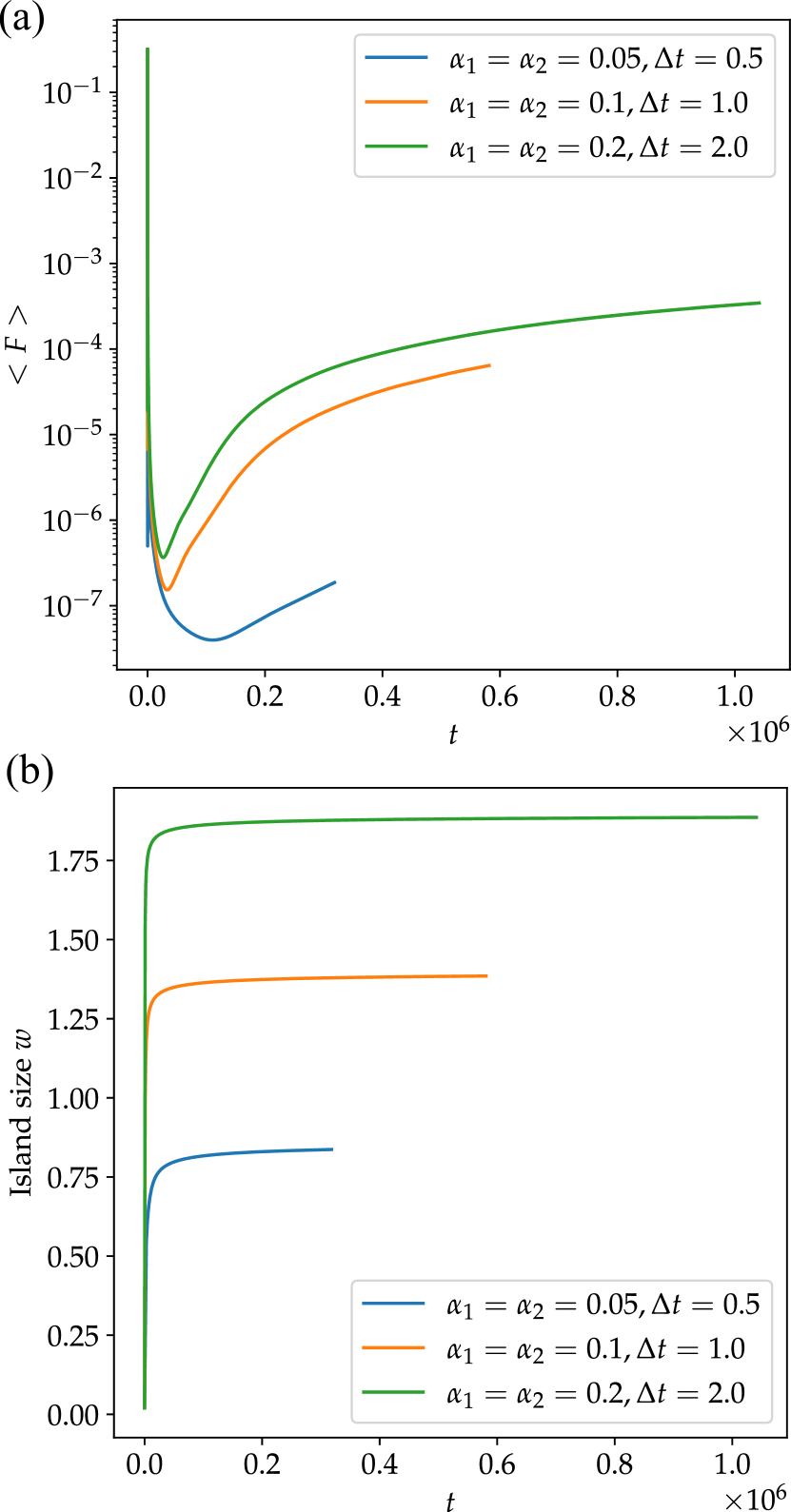
Figure 1: The averaged residual force (a) and the magnetic island size (b) versus time for runs with different Voigt coefficients and time steps.

Figure 2: A zoom-in view of the current density distribution near the X-point for the run with $\alpha_{1}=\alpha_{2}=0.1$ at a late time.

Now we apply the 2D Voigt-MHD code to some test problems. The first problem is to find an ideal MHD equilibrium, starting from a current sheet that is unstable to the tearing instability. We start from a one-dimensional equilibrium defined by[16]

$$\psi_{0}=a\left(\frac{1}{\cosh^{2}\left(y\right)}-1\right),$$ (25)

where the coefficient $a=3\sqrt{3}/4$. The corresponding current density is

$$J_{0}=a\left(\frac{2}{\cosh^{4}\left(y\right)}-\frac{4\tanh^{2}\left(y\right)}{\cosh^{2}\left(y\right)}\right).$$ (26)

Then we perturb the field by multiplying $\psi_{0}$ by a factor of $1+\epsilon\cos\left(2\pi x/L_{x}\right)$, where $\epsilon$ is a small parameter. This perturbation seeds a narrow island in the field.

In this set of runs, the resistivity $\eta$ and the external electric field $E_{\text{ext}}$ are set to zero. The Voigt term in the induction equation facilitates reconnection, allowing the island to grow. We set $L_{x}=4$, $L_{y}=2\pi,$ and $\epsilon=10^{-4}$. The resolution is $N_{x}=N_{y}=256$. The viscosity is set to $\nu=10^{-2}.$ We vary the Voigt coefficients for the following values $\alpha_{1}=\alpha_{2}=0.05,$ $0.1$, and $0.2$; the corresponding time steps are $\Delta t=0.5$, $1$, and $2$.

We test the convergence of the numerical solution toward the infinite-time asymptotic equilibrium by evaluating the averaged residual force over the whole volume

$$\left\langle F\right\rangle=\left\langle\left|-\nabla p+\boldsymbol{J}\times\boldsymbol{B}\right|\right\rangle.$$ (27)

Figure 1(a) shows the averaged residual force versus time for various runs. For all these runs, the averaged residual force initially tends to decrease rapidly, but eventually this tendency is arrested. Worse, the averaged residual force starts to increase gradually. As such, the numerical solutions of these runs do not appear to satisfactorily converge to asymptotic equilibria. Figure 1(b) plots the magnetic island size versus time for various runs, showing that the island size is still slowly growing at later times.

Inspecting the residual force distribution reveals that the unbalanced force is mostly localized along the separatrix near the X-point, where the current density $J$ becomes spiky (Figure 2). Inspecting the current density profile also suggests that this numerical calculation does not have sufficient resolution to resolve the spiky current density. Moreover, because the force balance condition $-\nabla p+\boldsymbol{J}\times\boldsymbol{B}=0$ in 2D implies $\boldsymbol{B}\cdot\nabla J=0$, the spiky $J$ near the X-point should spread out exactly along the separatrix such that $J=J\left(\psi\right)$. This condition is clearly not satisfied in Figure 2. To resolve this thin current structure, we must have high resolution not only near the X-point, but also along the separatrix. However, even if we have sufficient numerical resolution, the spreading of current density along the separatrix would likely take a long time.

Although our numerical solutions have not achieved desirable convergence and the magnetic island sizes are still slowly growing, it is clear that the final equilibrium depends on the Voigt coefficient $\alpha_{2}$. This fact can be inferred from Eq. (24) as follows. Because $\boldsymbol{u}=0$ at the X-point and the O-point, the quantity $\psi+\alpha_{2}J$ is time-independent at these two points. Neglecting the small initial seeded island, the reconnected magnetic flux is given by $\psi_{\text{O}}-\psi_{\text{X}}=\alpha_{2}\left(J_{\text{X}}-J_{\text{O}}\right)$, where the subscripts X and O specify the values evaluated at the X-point and the O-point, respectively. If the asymptotic solution is independent of $\alpha_{2}$, then both $\psi_{\text{O}}-\psi_{\text{X}}$ and $J_{\text{X}}-J_{\text{O}}$ are independent of $\alpha_{2}$, leading to a contradiction.

III.3 Resistive MHD Equilibria with External Electric Field

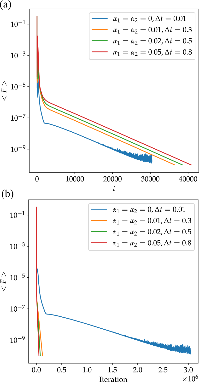
Figure 3: The averaged residual force versus time (a) and the number of iterations (b) for resistive tearing runs.

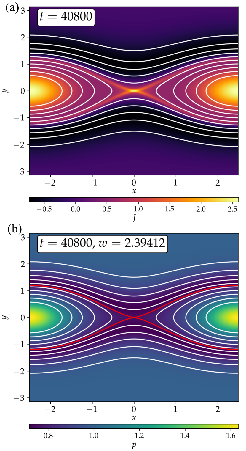
Figure 4: The current density (a) the pressure (b) distribution of converged equilibrium of the resistive tearing problem, from the calculation of $\alpha_{1}=\alpha_{2}=0.05$. White contours are samples of field lines, and the red contour denotes the saturated magnetic island.

Now we repeat the tearing mode problem by adding the resistivity. To prevent the solution from decaying to a vacuum field, an external electric field $E_{\text{ext}}=-\eta J_{0}$ is applied. For this set of runs, we set $\eta=\nu=10^{-3}$. The system size is given by $L_{x}=5$ and $L_{y}=2\pi$. The perturbation coefficient is $\epsilon=10^{-4}$. The resolution is $N_{x}=N_{y}=256$.

With a finite resistivity, the plasma flow in the final equilibrium no longer vanishes. Roughly speaking, the plasma flow is proportional to $\eta$. Because of the non-vanishing flow, the $\boldsymbol{u}\cdot\nabla\boldsymbol{u}$ term and the viscous term must be incorporated in the calculation of the averaged residual force:

$$\left\langle F\right\rangle=\left\langle\left|\nabla p+\boldsymbol{J}\times\boldsymbol{B}-\boldsymbol{u}\cdot\nabla\boldsymbol{u}+\nu\nabla^{2}\boldsymbol{u}\right|\right\rangle.$$ (28)

We vary the Voigt coefficients for the following values $\alpha_{1}=\alpha_{2}=0,$ $0.01$, $0.02$, and $0.05$; the corresponding time steps are $\Delta t=0.01$, $0.3,$ $0.5$, and $0.8$. Note that because of the flow, which ultimately limits the CFL condition, further increasing the Voigt coefficients does not allow significantly larger time-steps.

We run the simulations until the averaged residual force $\left\langle F\right\rangle\leq 10^{-10}$. Figure 3(a) shows the averaged residual force versus time for different Voigt coefficients. The results indicate that cases with larger Voigt coefficients take longer to converge with respect to the time variable. In practice, what really matters is the number of iterations it takes to obtain the converged solution. As can be seen in Figure 3 (b), cases with larger Voigt coefficients take fewer iterations to converge, because of the larger time-steps. Without Voigt regularization, it takes approximately three million iterations to achieve $\left\langle F\right\rangle<10^{-10}$, whereas with Voigt coefficients $\alpha_{1}=\alpha_{2}=0.05$, it takes approximately $51,000$ iterations for the same accuracy. That is approximately a factor of 60 speed-up.

The converged solutions are practically independent of the Voigt coefficients and time-steps. Figure 4 shows the current density and pressure distributions of the converged solution, obtained from the run with $\alpha_{1}=\alpha_{2}=0.05$, overlaid with field lines (white contours) and the outline of the magnetic island (red contours). The saturated island size $w\approx 2.3941$. Note that the current density near the X-point is smoother than the ideal case shown in Figure 2. Importantly, the presence of flow in the resistive case means the equilibrium no longer satisfies $\boldsymbol{B}\cdot\nabla J=0$, a condition that holds strictly in 2D ideal MHS equilibria. Therefore, the current density peak at the X-point does not exactly spread out along the separatrix.

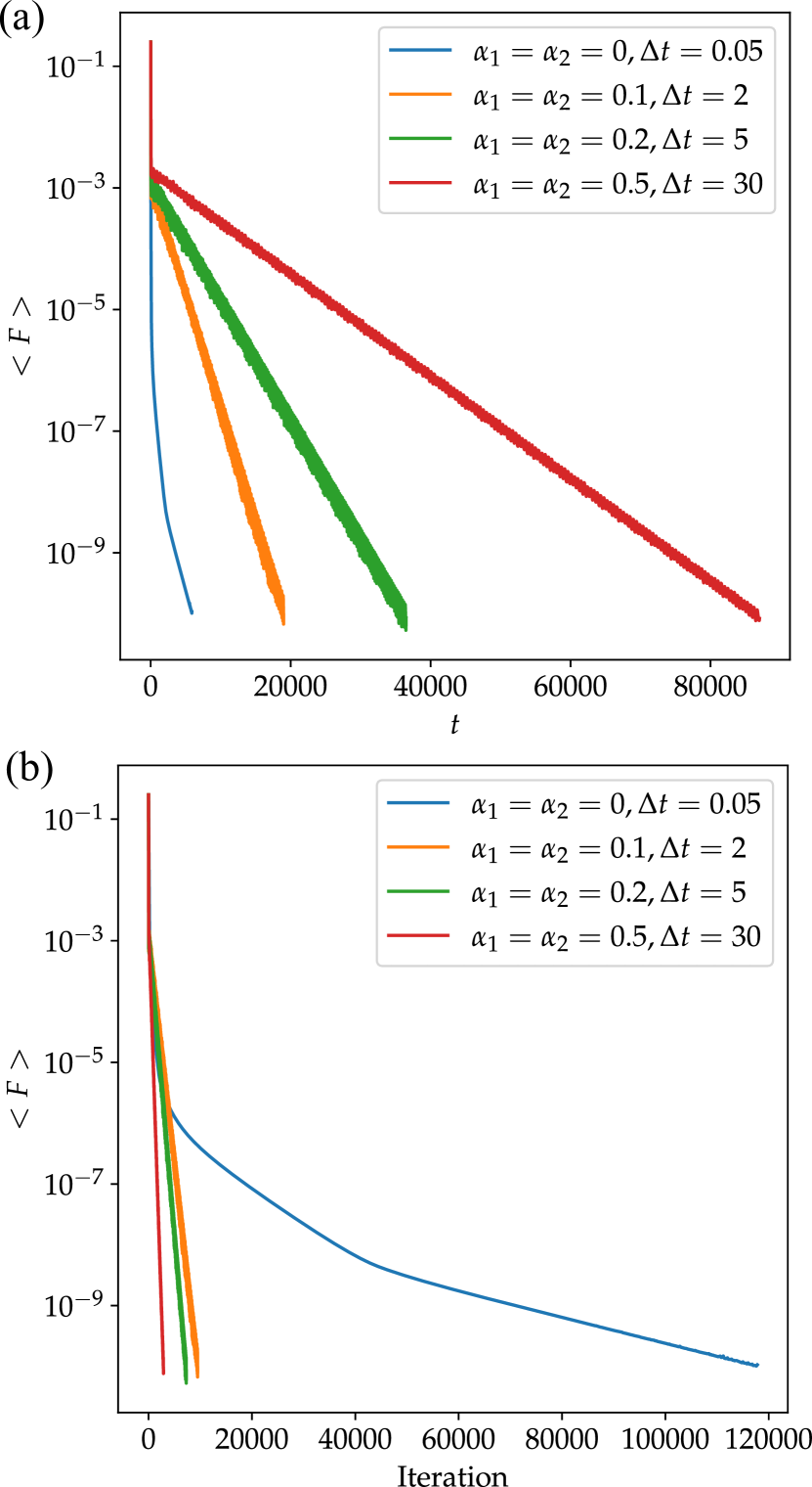
Figure 5: The averaged residual force versus time (a) and the number of iterations (b).

Figure 6: The pressure distribution of converged equilibrium of the HKT problem, from the calculation of $\alpha_{1}=\alpha_{2}=0$. White contours are samples of field lines, and the red contour denotes the saturated magnetic island.

The next test problem is the Hahm–Kulsrud–Taylor forced reconnection problem.[23] The initial condition is

$$\psi=\frac{1}{2}y^{2}\left(1+\epsilon\cos\left(2\pi x/L_{x}\right)\right),$$ (29)

corresponding to a uniformly sheared magnetic field $\boldsymbol{B}=y\boldsymbol{\hat{x}}$ with an added perturbation. We set $L_{x}=7$, $L_{y}=1,$ and $\epsilon=0.1$. The resolution is $N_{x}=N_{y}=128$. The viscosity and resistivity are set to $\eta=\nu=10^{-4}.$ We vary the Voigt coefficients for the following values $\alpha_{1}=\alpha_{2}=0,$ $0.1$, $0.2$, and $0.5$. The corresponding time-steps are $\Delta t=0.05$, $2$, $5$, and $30$. In this example, the plasma velocity asymptotically goes to zero. Therefore, the CFL condition is only limited by waves, and we can use much larger time-steps with the Voigt regularization.

We again run the simulations until the averaged residual force $\left\langle F\right\rangle\leq 10^{-10}$. Figure 5(a) shows the averaged residual force versus time for different Voigt coefficients. Again, cases with larger Voigt coefficients take longer to converge with respect to the time variable. On the other hand, as shown in Figure 5 (b), cases with larger Voigt coefficients take fewer iterations to converge, because of the larger time steps. Without Voigt regularization, it takes approximately $120,000$ iterations to achieve $\left\langle F\right\rangle<10^{-10}$, whereas with Voigt coefficients $\alpha_{1}=\alpha_{2}=0.5$, it only takes approximately $2,900$ iterations for the same accuracy, corresponding to a factor of 40 speed-up.

The converged solutions are again independent of the Voigt coefficients and time steps. Figure 6 shows the pressure profile of the converged solution, obtained from the run without Voigt regularization, overlaid with field lines (white contours) and the outline of the magnetic island (red contours). The saturated island size $w\approx 0.427872$.

IV Conclusions and Future Perspectives

In summary, this study represents the first investigation of Voigt regularization for obtaining MHD equilibria, demonstrating its potential for accelerating the convergence to solutions in resistive MHD problems while also highlighting challenges in applying the method to ideal MHD systems.

Despite the theorem of Constantin and Pasqualotto guaranteeing regular time-asymptotic solutions, our calculations of ideal MHD equilibria encounter difficulties in achieving full convergence, primarily due to insufficient resolution of the spiky current density near the X-point. Moreover, the strict requirement of current density being constant along magnetic field lines in 2D ideal MHS equilibria, coupled with the spiky current density at the X-point, may also require an impractically long time to relax to an equilibrium.

In contrast, our numerical experiments demonstrate that Voigt regularization can be a powerful technique to obtain resistive MHD equilibria with an external electric field. Because the Voigt terms slow down MHD waves, thereby allowing larger time-steps, the convergence to equilibrium solutions is significantly accelerated without affecting the final equilibrium state.

Our resistive MHD test problems serve as prototypes for more general problems incorporating transport effects and source terms. Examples include problems of slowly diffusing resistive equilibrium with particle sources[27, 28, 29] or problems with thermal conduction and heat sources. In practice, equilibria with sources and transports are physically more relevant than ideal MHD equilibria. Plasma flow that naturally arises in this type of equilibria may also mitigate some of the problems caused by the restrictions of ideal MHD equilibria, such as the strict enforcement of $\boldsymbol{B}\cdot\nabla p=0$ and $\boldsymbol{B}\cdot\nabla J=0$ (in 2D).

Many questions remain open for future investigations. An immediate next step is to increase the resolution in the ideal MHD test problem in Section III.2 to see if converged solutions can be obtained, perhaps using adaptive mesh refinemnt techniques.[30] Three-dimensional generalizations of the problem that allow formation of chaotic field line region should be attempted, as that could help alleviate some difficulties in Section III.2 due to 2D symmetry. Another question we have not explored deeply is how to optimally choose Voigt coefficients and time-steps to achieve fast convergence with a small number of iterations. Techniques such as pseudotransient continuation may further improve the convergence speed.[31] Finally, a generalization of Voigt regularization to compressible MHD, incorporating transports and various sources, should be explored. This could lead to development of more efficient and physically relevant MHD equilibrium solvers, further contribute to the design and optimization of future fusion devices.