Dyonic Taub-NUT-AdS Black Branes:
Thermodynamics and Phase Diagrams

Abstract

Motivated by the recent developments in the thermodynamics of Taub-NUT spaces and the absence of Misner strings in Taub-NUT solutions with flat horizons, we investigated the phase structure of dyonic Taub-NUT solutions. We follow the treatment proposed in arXiv:2206.09124 and arXiv:2304.06705 to introduce the nut parameter as a conserved charge to the first law. Although the calculated quantities satisfy the first law, we have found a larger class of charges that satisfy the first law and depend on some arbitrary parameter which we call $\alpha$. We choose to describe phase diagrams as NUT parameter-Temperature graphs to show borders of big and small black hole phases. We study the phase structure of these spaces in a mixed ensemble (i.e., we fix the electric potential, the nut parameter, and the magnetic charge), which we classify into different cases depending on the value of $\alpha$. In some of these cases we have first-order phase transitions that end with critical points. These classes could include up to four critical points, again, depending on $\alpha$ and the other quantities.

1 Introduction

One of the most attractive features of anti-de Sitter space solutions is the possibility of having positive specific heat [1]. This reflects the thermal stability of these AdS solutions in contrast to flat space solutions with negative specific heat. In their work, Hawking and Page [1] were able to show the existence of a phase transition between the black hole and the pure thermal AdS phases. Later, this was interpreted as the transition between the confinement and deconfinement phases of the dual gauge theory in the context of AdS/CFT correspondence [2]. After a year, this was extended to the AdS charged black hole [3, 4] where the authors found first-order phase transitions ending at a critical point, a very similar behavior to the well known liquid-gas phase transition.

Indeed, Working in AdS spaces enlarges the spectrum of various types of black holes, since they come with three horizon topologies; spherical, flat, or hyperbolic. Therefore, it is interesting to study the thermodynamics of AdS black holes with a flat horizon, which was investigated in [5, 6, 7]. Furthermore, their extended thermodynamics was studied in [8] as well. However, these investigations showed no sign of first-order phase transitions or critical behavior since the black hole horizon temperature varies monotonically as a function of the horizon radius! This is why some authors tried to use unconventional methods to obtain a system with a non-trivial phase diagram as in [9, 10, 11, 12]. In [9, 10, 11], for example, the authors introduced a complex scalar field that gave rise to a superconductor phase diagram with a second-order phase transition between a black brane with scalar hair at low temperature and a black brane with no hair at high temperature. In [12], on the other hand, the authors achieved phase transition and critical behavior by introducing higher curvature terms with certain topological features to the gravitational action.

One of the attractive classes of solutions studied in this duality is the AdS-Taub-Bolt/NUT black holes in four and higher dimensions [13, 14, 15, 16]. This class of solutions is a generalization to the Schwarzschild-AdS space with one additional parameter, the nut charge ”n”. An important feature of these solutions is that they possess string-like singularities known as Misner strings[17]. These strings are analogous to the Dirac string in electromagnetism and can be removed by imposing certain periodicity conditions, namely; the inverse temperature set to be $\beta=8\pi n$. In [13, 18, 14, 19, 20] the thermodynamics was studied and the authors revealed unusual features of these solutions. For example, the entropy is not the area of the horizon, even not always positive, and the horizon temperature and radius are fixed by the nut parameter n. Another unusual property of these solutions is that there are no additional terms in the first law due to the above relation between the nut charge and the horizon radius.

Motivated by some recent suggestions on the Taub-NUT thermodynamics [21, 22, 23, 24, 25, 26, 27, 28, 29, 30, 31, 32, 33, 34, 35] several authors tried to probe the possibility of relaxing the above periodicity condition, leaving the Misner string visible and allowing the NUT charge to appear in the first law as an independent charge with its conjugate potential.

In this work we study the regular thermodynamics of dyonic black branes with a non-vanishing NUT charge using the treatment introduced in [30, 33] where the authors introduced the NUT charge as a conserved charge which contributes to the first law with an extra work-term. Also, in [33], the authors found mass, angular momentum, NUT, electric, and magnetic charge densities distributed along Misner string when studying the dyonic Taub-NUT black hole solution. In fact, relaxing the periodicity condition was first considered by Bonner in [36] where he showed that the string singularity is a source of angular momentum.
In this study, we closely follow the approach outlined in [34], but with two major differences. Firstly, instead of focusing on black holes with spherical horizons, we will be examining black holes with flat horizons, also known as ”black branes”. Secondly, while authors in [34] studied the extended thermodynamics of black holes, which includes considerations such as varying the cosmological constant as a thermodynamic variable, our study will focus on the regular thermodynamics of black branes. We show that allowing the dyonic black brane to have a non-vanishing NUT charge while relaxing the Misner periodicity condition results in a consistent thermodynamics where the Gibbs-Duhem relation and the first law are both satisfied, the entropy is related to the horizon area, and the temperature goes to that of the NUT-less case as $n\rightarrow 0$. We also show that the phase diagram becomes nontrivial in this case, with first-order phase transitions, continuous phase transitions, and critical behavior taking place.

The paper is organized as follows; in section (2) we revisit the NUT-less dyonic black brane showing that its phase diagram is indeed trivial with no signs of phase transitions or critical behavior. In section (3) we study the Taub-NUT dyonic black brane, studying the regular thermodynamics of the mixed ensemble of the solution by calculating its thermodynamic quantities and showing that they alongside an arbitrary parameter $\alpha$ satisfy the first law and the Gibbs-Duhem relation in subsection (3.1), In (3.2) we divide the general case into sub-cases depending on the values of the thermodynamic quantities and studying the phase transitions and the phase diagram for each case. Finally in section (4) we discuss our treatment and present our conclusion while outlining possible extensions and future directions.

2 NUT-less Dyonic AdS Black Brane

The metric of the dyonic black brane in AdS space is given by

$$ds^{2}=-f(r)\,dt^{2}\,+\,\frac{dr^{2}}{f(r)}\,+\,\frac{r^{2}}{l^{2}}\,(\,dx^{2}+\,x^{2}\,d\varphi^{2}),$$ (1)

here $x\in[0,A]$, $\varphi\in[0,2\pi]$, and $l$ is the anti-de-Sitter radius given by $l=\sqrt{-\frac{3}{\Lambda}}$ where $\Lambda$ is the cosmological constant. The area of the brane is given by

$$\int_{0}^{2\pi}\int_{0}^{A}\frac{1}{l^{2}}\,x\,dx\,d\phi=\frac{\pi A^{2}}{l^{2}}=4\pi\sigma.$$ (2)

And $f(r)$ is given by

$$f(r)\,=\,\frac{r^{2}}{l^{2}}\,+\,\frac{q^{2}\,+p^{2}}{r^{2}}\,-\,\frac{2\,m}{r}\,.$$ (3)

Here $m$, $q$, and $p$ are constants, but as we will show in a short while they are related to the mass and charge densities of the brane.

From the horizon condition, $f(r_{h})=0$, the mass parameter, $m$, of the brane is given by

$$m=\frac{1}{2}\left(\frac{r_{h}^{3}}{l^{2}}+\frac{q^{2}+p^{2}}{r_{h}}\right),$$ (4)

The non-vanishing components of the gauge potential $A_{\mu}$ are given by

$$A_{t}\,=\,V-\frac{q}{r},$$ (5)

and

$$A_{\varphi}\,=\,\frac{p\,x^{2}}{2\,l^{2}}.$$ (6)

The square of the gauge potential, $A_{\mu}A^{\mu}$, is given by

$$A_{\mu}A^{\mu}\,=\,\frac{p^{2}\,x^{2}}{4\,r^{2}\,l^{2}}\,-\,\frac{(r\,V\,-\,q)^{2}}{r^{2}\,f(r)}.$$ (7)

To prevent $A_{\mu}A^{\mu}$ from blowing up at the horizon (see [37, 38]), $q$ must be related to $V$ in the following way

$$q\,=\,r_{h}\,V,$$ (8)

The electric and magnetic potentials can be calculated as follows

$$\phi_{e}\,=\,A_{t}|_{\infty}\,-\,A_{t}|_{r_{h}}\,=V=\frac{q}{r_{h}},$$ (9)

$$\phi_{m}\,=\,B_{t}|_{\infty}\,-\,B_{t}|_{r_{h}}=\frac{p}{r_{h}}.$$ (10)

Where the one form $B$ is the solution for $dB\,=\,*F$, where $*F$ is the Hodge dual of $F$, given by

$$(*F)_{\mu\nu}=\frac{1}{2}\,\epsilon^{\,\alpha\beta}_{\>\>\,\>\>\>\mu\nu}\,F_{\alpha\beta},$$ (11)

where $\epsilon$ is the Levi-Civita tensor. The electric and magnetic charge densities are calculated using Stokes’ theorem.

$$Q_{e}=\frac{1}{4\pi\sigma}\int_{\partial\Sigma}*F\,=\,q,$$ (12)

$$Q_{m}=-\frac{1}{4\pi\sigma}\int_{\partial\Sigma}F\,=\,p.$$ (13)

We must be careful when dealing with the boundary surface $\partial\Sigma$, as it is not simply the surface of constant $r$, but also consists of the surface of constant $x$.

Figure 2.1: The boundary of spacetime at spatial infinity. the boundary consists of the top cape of $r=\infty$ and the side of the cone at $x=A$ from $r=r_{h}$ to $r=\infty$. The dashed line represents the hypersurface of $r=r_{h}$.

From Eq.(12) and Eq.(13) we can see that $q$ and $p$ are proportional to the brane’s electric and magnetic charges per unit area, $\sigma$, respectively.

2.1 Thermodynamics

The Euclidean path integral boundary conditions fix the boundary metric and the spatial component of the gauge potential, which in turn fixes the electric potential and the magnetic charge density. Therefore, the ensemble in hand is a mixed ensemble with the partition function $Z=Z(T,\phi_{e},Q_{m})$ [38, 37].

The temperature of the horizon is calculated by performing a Wick rotation to the metric, with the temperature equal to the inverse of the periodicity of the imaginary time coordinate [39, 40, 38]

$$T_{h}\,=\,\frac{f^{\prime}(r)}{4\,\pi}\biggr{|}_{r=r_{h}}\,=\,\frac{1}{\,4\,\pi\,r_{h}}\left(\frac{3\,r_{h}^{2}}{l^{2}}-\frac{Q_{m}^{2}}{r_{h}^{2}}-\phi_{e}^{2}\right).$$ (14)

From Eq.(14) we can see that regardless of the values of $Q_{m}$ and $\phi_{e}$, the temperature is always a monotonic function in the horizon radius. This can be seen in Fig. 2.2.

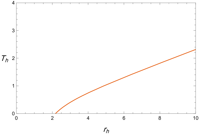
Figure 2.2: The temperature of the dyonic black brane as a function of its horizon radius for $Q_{m}=5$ and $\phi_{e}=3$. The graph shows that for any temperature, there exists only one possible black brane solution.

Moreover, we can see that there is always an extremal solution with radius $r_{e}$, where

$$r_{e}=\frac{\sqrt{6l^{2}\,\phi_{e}^{2}\,+\,6\,\sqrt{l^{4}\,\phi_{e}^{4}\,+\,12l^{2}Q_{m}^{2}}}}{6}.$$ (15)

As $f^{\prime}(r)\Bigr{|}_{r=r_{e}}=0$, the solution will not develop any conical singularity when the metric is Wick rotated. Therefore, the solution can have any arbitrary temperature, meaning it can exist at any temperature in that regard. However, as the surface gravity of the extremal black branes also vanishes, we do not expect that the extremal black brane can really exist at any temperature other than $T=0$. Indeed, we will find that at any non-zero temperature, there will always exist another solution with a lower grand potential density.

To calculate the grand potential density, one must first calculate the on-shell gravitational action. We will be calculating the on-shell action of the solution using the counter-term method [14] such that

$$I=I_{b}+I_{s}+I_{ct},$$ (16)

where $I_{b}$ is the Einstein-Hilbert action with negative cosmological constant and the electromagnetic contribution to the action which is given by

$$I_{b}=-\frac{1}{16\pi}\int_{\mathcal{M}}d^{4}x\,\sqrt{-g}\,(R-2\Lambda-F_{\mu\nu}F^{\mu\nu}),$$ (17)

and $I_{s}$ is the Gibbons–Hawking–York boundary term given by

$$I_{s}=-\frac{1}{8\pi}\int_{\partial\mathcal{M}}d^{3}x\,\sqrt{-h}\,K,$$ (18)

where $h$ is the determinant of the boundary metric and $K$ is the trace of the boundary’s extrinsic curvature $K^{\alpha\beta}$. The integral $I_{ct}$ is the counter-term to cancel the divergences that arise from integrating over an infinite AdS volume, which is given by

$$I_{ct}=\frac{1}{8\pi}\int_{\partial\mathcal{M}}d^{3}x\,\sqrt{-h}\,\left(\frac{2}{l}+\frac{l}{2}\mathcal{R}\right),$$ (19)

where $\mathcal{R}$ is the Ricci scalar for the boundary metric. The on-shell action density is evaluated to give

$$\mathcal{J}=\frac{I}{\sigma}=\beta\,\Omega=\frac{\beta}{2}\left(m+\frac{p^{2}-q^{2}}{r_{h}}-\frac{r_{h}^{3}}{l^{2}}\right)=\frac{\beta}{4}\left(\frac{3\,p^{2}}{r_{h}}-\frac{r_{h}^{3}}{l^{2}}-\phi_{e}^{2}r_{h}\right).$$ (20)

Where $\,\Omega\,$ is the grand potential density, which equals $\mathcal{J}/\beta$. The entropy density of the system can be calculated from the on-shell action density as follows

$$S=\beta\,\partial_{\beta}\mathcal{J}-\mathcal{J}=\pi r_{h}^{2},$$ (21)

which is consistent with the entropy being one-quarter of the black brane area. Moreover, the variation of $\,\Omega\,$ is consistent with Gibbs-Duhem relation

$$\mathrm{d}\Omega\,=\,-S\,\mathrm{d}T\,-\,Q_{e}\,\mathrm{d}\phi_{e}\,+\,\phi_{m}\,\mathrm{d}Q_{m},$$ (22)

with

$$\left(\frac{\partial{\Omega}}{\partial{T}}\right)_{\phi_{e},Q_{m}}=-S,\quad\left(\frac{\partial{\Omega}}{\partial{\phi_{e}}}\right)_{T,Q_{m}}=-Q_{e},\quad\left(\frac{\partial{\Omega}}{\partial{Q_{m}}}\right)_{T,\phi_{e}}=\phi_{m}.$$ (23)

Also, the total energy density of the solution can be calculated from the on-shell action density as follows

$$\mathfrak{M}=\partial_{\beta}\mathcal{J}\,+\,Q_{e}\,\phi_{e}=\frac{1}{2}\left(\frac{r_{h}^{3}}{l^{2}}+\frac{Q_{m}^{2}}{r_{h}}+\phi_{e}^{2}\,r_{h}\right)=m,$$ (24)

which means that $m$ is also proportional to the mass per unit area of the brane. The total energy density of the solution is also consistent with the first law

$$\mathrm{d}\mathfrak{M}=T\mathrm{d}S+\phi_{e}\,\mathrm{d}Q_{e}+\phi_{m}\,\mathrm{d}Q_{m},$$ (25)

with

$$\left(\frac{\partial{\mathfrak{M}}}{\partial{S}}\right)_{Q_{e},Q_{m}}=T,\quad\left(\frac{\partial{\mathfrak{M}}}{\partial{Q_{e}}}\right)_{S,Q_{m}}=\phi_{e},\quad\left(\frac{\partial{\mathfrak{M}}}{\partial{Q_{m}}}\right)_{S,Q_{e}}=\phi_{m}.$$ (26)

Next, we need to check the thermal stability of the black brane. We can see that the slope of the temperature curve is positive everywhere, Fig. 2.2, indicating that the black brane is thermally stable at any temperature.

To see that the dyonic black brane solution is always more thermodynamically preferable than its extremal solution as we mentioned earlier, the grand potential densities of both solutions are plotted in Fig. 2.3. it is clear from the Fig. that the dyonic black brane solution is always the most thermodynamically preferable solution for any non-zero value of the horizon temperature.

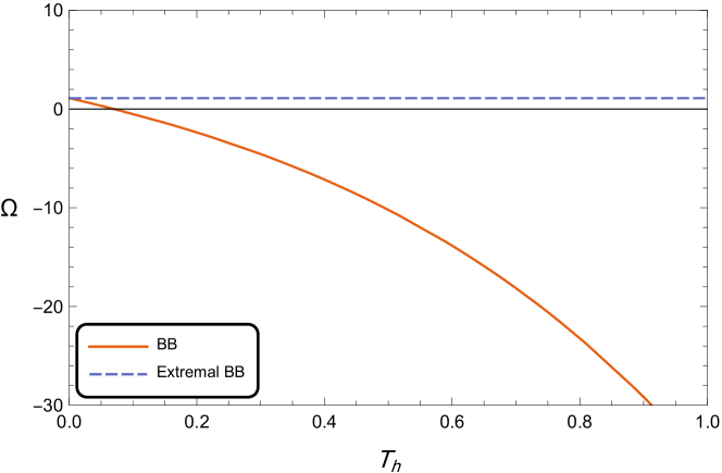
Figure 2.3: The grand potential densities of the possible phases as functions of their horizon temperature for $Q_{m}=5$ and $\phi_{e}=3$, the solid line represents the dyonic black brane, while the dotted line represents the extremal dyonic black brane. The graph shows that for any temperature the black brane solution always has a lower grand potential than the extremal black brane.

We can clearly see that for NUT-less dyonic black branes, the phase diagram is always trivial and phase transitions do not occur. In the next section, we will investigate the solution where the NUT charge is not zero to check if this will render a non-trivial phase structure.

3 Taub-NUT Dyonic AdS Black Brane

Now we will take a look at the same solution but with a non-vanishing NUT charge. More crucially, as we mentioned in the introduction, we will follow the same approach as in [34], where we relax the periodicity condition for the time coordinate, making the NUT charge a true independent charge that appears in the first law alongside its conjugate quantity $\phi_{n}$.

The metric for the Taub-Nut dyonic AdS black brane is given by

$$ds^{2}=-f(r)\,\left(dt\,-\,\frac{nx^{2}}{l^{2}}\,d\varphi\right)^{2}+\,\frac{dr^{2}}{f(r)}\,+\,\frac{r^{2}+n^{2}}{l^{2}}\,(\,dx^{2}+\,x^{2}\,d\varphi^{2}),$$ (27)

where the area of the brane and the ranges of both $x$ and $\phi$ are the same as those in the NUT-less case. The function $f(r)$ is now given by

$$f(r)\,=\,\frac{q^{2}+p^{2}-2\,m\,r}{r^{2}+n^{2}}\,+\,\frac{r^{4}+6\,n^{2}\,r^{2}-3\,n^{4}}{\left(r^{2}+n^{2}\right)\,l^{2}}.$$ (28)

Again, $m$, $q$, and $p$ are constants. The proper mass and charge densities will be calculated later.

Using $f(r_{h})=0$, the mass parameter, $m$, is related to the other parameters by

$$m=\frac{l^{2}\left(q^{2}+p^{2}\right)\,+\,r_{h}^{4}+6\,n^{2}\,r_{h}^{2}-3\,n^{4}}{2l^{2}r_{h}}.$$ (29)

The non-vanishing components of the gauge potential $A_{\mu}$ are

$$A_{t}=\frac{pn-qr}{r^{2}+n^{2}}+V,$$ (30)

and

$$A_{\varphi}=\frac{p\left(r^{2}-n^{2}\right)+2qnr}{2\,l^{2}\,\left(r^{2}+n^{2}\right)}\,x^{2},$$ (31)

To guarantee that the square of the gauge potential, $A_{\mu}A^{\mu}$, is regular at the horizon, the parameters $q$, $n$, and $V$ must be related through the relation

$$q\,=\,\frac{pn+V\left(r_{h}^{2}+n^{2}\right)}{r_{h}},$$ (32)

The electric and magnetic potentials are calculated from the relations

$$\phi_{e}\,=\,A_{t}|_{\infty}\,-\,A_{t}|_{r_{h}}\,=V$$ (33)

$$\phi_{m}\,=\,B_{t}|_{\infty}\,-\,B_{t}|_{r_{h}}=\frac{p+nV}{r_{h}}.$$ (34)

The electric and magnetic charge densities are calculated using Stokes’ theorem

$$Q_{e}=\frac{1}{4\pi\sigma}\int_{\partial\Sigma}*F,\quad\,Q_{m}=-\frac{1}{4\pi\sigma}\int_{\partial\Sigma}F$$ (35)

As seen before, the hypersurface at spatial infinity consists of two parts; the surface of constant $r$ with $r=\infty$ and $x\in[0,A]$, and the surface of constant $x$ with $x=A$ and $r\in[r_{h},\infty]$. The electric and magnetic charge densities are then given by

$$Q_{e}=\frac{1}{4\pi\sigma}\int_{0}^{2\pi}\int_{0}^{A}(*F)_{x\phi}\,\mathrm{d}x\mathrm{d}\phi\,+\frac{1}{4\pi\sigma}\int_{r_{h}}^{\infty}\int_{0}^{2\pi}(*F)_{\phi r}\,\mathrm{d}\phi\mathrm{d}r$$

$$=q-2n\phi_{m},$$ (36)

and,

$$Q_{m}=-\frac{1}{4\pi\sigma}\int_{0}^{2\pi}\int_{0}^{A}(F)_{x\phi}\,\mathrm{d}x\mathrm{d}\phi\,-\frac{1}{4\pi\sigma}\int_{r_{h}}^{\infty}\int_{0}^{2\pi}(F)_{\phi r}\,\mathrm{d}\phi\mathrm{d}r$$

$$=p+2n\phi_{e}.$$ (37)

In fact, if we choose the boundary at any generic radial distance with $r\,>\,r_{h}$, we will get the same results for the electric and magnetic charge densities. This is a very interesting result. Unlike the NUT-less case where there was no flux through the constant $x$ hypersurface, we get here an $r$-dependent electric and magnetic charge densities if we considered the surfaces of constant $r$ for any generic radial distance with $r>r_{h}$. This is a consequence of the flux leaking through the constant $x$ surface.

We can also calculate the conserved NUT charge density, $N$, as the dual to the mass density by the generalized Komar integral [41, 21]

$$N=\frac{1}{4\pi\sigma}\int_{\partial\Sigma}\mathrm{d}\xi-2\Lambda(*\omega)=\frac{4n^{3}}{l^{2}},$$ (38)

where $\xi=\partial_{t}$ is a time-like Killing vector and $\omega$ is the Killing potential satisfies $\xi^{\mu}=\nabla_{\nu}\omega^{\nu\mu}$ or $d\omega=*\xi$.

3.1 Thermodynamics

As discussed previously in the NUT-less case, the Euclidean path integral boundary conditions fix the electric potential and the magnetic charge density. In the NUTty case, they in addition fix the NUT charge density, $N$. The ensemble therefore is also a mixed ensemble with the partition function $Z=Z(T,\phi_{e},Q_{m},N)$ [30].

The temperature of the brane is given by

$$T_{h}\,=\,\frac{f^{\prime}(r)}{4\,\pi}\,=\frac{\left(3r_{h}^{2}-l^{2}\phi_{e}^{2}\right)\left(r_{h}^{2}+n^{2}\right)-l^{2}p\left(p+2n\phi_{e}\right)}{4\pi l^{2}r^{3}_{h}}.$$ (39)

As in the NUT-less case, we calculate the on-shell action density using the counter-term method, which yields

$$\mathcal{J}=\frac{I}{\sigma}=\beta\,\Omega=\frac{\beta}{2}\left(m-q\phi_{e}+\frac{\left(p+n\phi_{e}\right)\left(p+2n\phi_{e}\right)}{r_{h}}-\frac{r_{h}\left(r_{h}^{2}+3n^{2}\right)}{l^{2}}\right).$$ (40)

The entropy density of the system is given by

$$S=\beta\,\partial_{\beta}\mathcal{J}-\mathcal{J}=\pi\left(r_{h}^{2}+n^{2}\right),$$ (41)

which is consistent with being one-quarter of the brane area.

Earlier we calculated the conserved NUT charge density to be $\,N=\frac{4n^{3}}{l^{2}}$. Given that we are doing a regular treatment to the thermodynamics, i.e. the cosmological constant is not allowed to vary and $l$ is constant, $n$ is consequently a conserved quantity. For the convenience of calculations, from now on we will continue our treatment using the conserved quantity $n$.

It is important to see that the charge densities calculated earlier, $Q_{e}=\left(q-2n\phi_{m}\right)$ and $Q_{m}\,=\,\left(p\,+\,2n\phi_{e}\right)$, do not satisfy the first law and the Gibbs-Duhem relation. In fact, if we set the electric charge density to be $Q_{e}$, the magnetic charge density that satisfies the first law and the Gibbs-Duhem relation is $p$. And if we set the magnetic charge density to $Q_{m}$, the electric charge that satisfies the two relations is nothing but $q$. In short, to satisfy these relations one of the charges must be the charge at infinity and the other one the charge at the horizon! This fact was previously reported by several authors [22, 23, 27, 30, 33, 34, 35]. Two of these authors [23, 33] showed that there exist an infinite family of electric and magnetic charge densities that satisfy both relations. The two charge densities can be parameterized by a real parameter $\alpha$, in the following forms:

$$\widetilde{Q}_{e}(\alpha)=q+\left(\alpha-1\right)n\phi_{m},$$ (42)

$$\widetilde{Q}_{m}(\alpha)=p+(\alpha+1)n\phi_{e}.$$ (43)

Here we follow the same approach adopted in [33, 34] where the authors applied it to the dyonic Taub-NUT black holes with spherical horizons. However, in the case of the spherical horizon, $\alpha$ is fixed to some value that leaves the gauge potential regular along the Misner string. In our case, with a flat horizon, the lack of a Misner string allows $\alpha$ to become a free parameter. Later, we will see how the different choices of $\alpha$ affect the phase diagram of the solution. For now, the charges given by Eq.(42) and Eq.(43) are consistent with the Gibbs-Duhem relation

$$\mathrm{d}\Omega=-S\mathrm{d}T-\widetilde{Q}_{e}\mathrm{d}\phi_{e}+\phi_{m}\mathrm{d}\widetilde{Q}_{m}+\phi_{n}\mathrm{d}n$$ (44)

with

$$\left(\frac{\partial{\Omega}}{\partial{T}}\right)_{\phi_{e},\widetilde{Q}_{m},n}=-S,\quad\left(\frac{\partial{\Omega}}{\partial{\phi_{e}}}\right)_{T,\widetilde{Q}_{m},n}=-\widetilde{Q}_{e},$$

$$\left(\frac{\partial{\Omega}}{\partial{\widetilde{Q}_{m}}}\right)_{T,\phi_{e},n}=\phi_{m},\quad\left(\frac{\partial{\Omega}}{\partial{n}}\right)_{T,\phi_{e},\widetilde{Q}_{m}}=\phi_{n},$$ (45)

where $\phi_{n}$ is given by

$$\phi_{n}=\frac{1}{2\,n\,r_{h}}\bigg{(}\frac{3\,n^{2}-l^{2}\phi_{e}^{2}}{l^{2}}\left(r_{h}^{2}-n^{2}\right)-r_{h}^{2}\,\phi_{e}^{2}\left(\alpha^{2}-1\right)\\ +\frac{1}{\,r_{h}^{2}}\left(n\,\widetilde{Q}_{m}-\,\alpha\,\phi_{e}\left(r_{h}^{2}+n^{2}\right)\right)^{2}\bigg{)}.$$ (46)

Finally, the total energy density of the solution can be calculated from the on-shell action density as follows

$$\mathfrak{M}=\partial_{\beta}\mathcal{J}\,+\,\widetilde{Q}_{e}\,\phi_{e},$$ (47)

which evaluates to

$$\mathfrak{M}=\frac{r_{h}\left(r_{h}^{2}+3n^{2}\right)}{2l^{2}}+\frac{\widetilde{Q}_{m}^{2}+\phi_{e}^{2}\left(r_{h}^{2}-\alpha^{2}n^{2}\right)}{2r_{h}}=m-n\phi_{n}.$$ (48)

this satisfies the first law

$$\mathrm{d}\mathfrak{M}=T\mathrm{d}\,S+\phi_{e}\,\mathrm{d}\widetilde{Q}_{e}+\phi_{m}\,\mathrm{d}\widetilde{Q}_{m}+\phi_{n}\,\mathrm{d}n,$$ (49)

with

$$\left(\frac{\partial{\mathfrak{M}}}{\partial{S}}\right)_{\widetilde{Q}_{e},\widetilde{Q}_{m},n}=T,\quad\left(\frac{\partial{\mathfrak{M}}}{\partial{\widetilde{Q}_{e}}}\right)_{S,\widetilde{Q}_{m},n}=\phi_{e},$$

$$\left(\frac{\partial{\mathfrak{M}}}{\partial{\widetilde{Q}_{m}}}\right)_{S,\widetilde{Q}_{e},n}=\phi_{m},\quad\left(\frac{\partial{\mathfrak{M}}}{\partial{n}}\right)_{S,\widetilde{Q}_{e},\widetilde{Q}_{m}}=\phi_{n}.$$ (50)

We notice from Eq.(48) that unlike the NUT-less case, where the total energy density is just $m$, there exists an extra term here, $n\phi_{n}$, which also contributes to the total energy density of the solution.

The temperature written in terms of the independent thermodynamic quantities takes the form

$$T_{h}\,=\frac{3\left(r_{h}^{2}+n^{2}\right)}{4\pi l^{2}r_{h}}-\frac{r_{h}^{2}\phi_{e}^{2}+\left(\widetilde{Q}_{m}-\alpha n\phi_{e}\right)^{2}}{4\pi r^{3}_{h}}.$$ (51)

In the next subsection, we will show that the phase diagram of the NUTty solution contains 0, 1, 2, or 4 critical points, in contrast to Nutless case. The number of critical points depends on the values of $\alpha$, $\widetilde{Q}_{m}$, and $n$. The other free parameters of the solution, $l$ and $\phi_{e}$, only scale the phase diagram by changing the values of $\alpha$, $\widetilde{Q}_{m}$, and $n$ where critical behavior occurs. Therefore, we can choose the values of $l$ and $\phi_{e}$ arbitrarily without losing any generality.

3.2 Phase Transitions and Critical Points

Since the Dyonic Nutless case has no phase transitions to compare it to the present cases, we find it convenient to construct the phase diagram as a $n-T$ diagram. The values of $\alpha$ and $\widetilde{Q}_{m}$ will affect and characterize these phase diagrams.

Before starting our analysis, we can notice that the signs of $\alpha$ and $\widetilde{Q}_{m}$ only affect the term $\left(\widetilde{Q}_{m}-\alpha n\phi_{e}\right)^{2}$. If both $\alpha$ and $\widetilde{Q}_{m}$ switch signs, the system is unaffected, but if only one of $\alpha$ or $\widetilde{Q}_{m}$ switches sign, we will get a system where $n\longrightarrow-n$. In the following analysis we will use positive values for $\alpha$ and $\widetilde{Q}_{m}$ knowing that we are not losing any generality.

3.2.1 Case I: $\alpha=0$

For $\alpha=0$, the $n-T$ phase diagram will only depend on the value of $\widetilde{Q}_{m}$. Generally, we have two cases;

Case I.I: $\widetilde{Q}_{m}=0$

When fixing the values of $\alpha$ and $\widetilde{Q}_{m}$ to zero, the horizon temperature will take the form

$$T_{h}\,=\frac{3\left(r_{h}^{2}+n^{2}\right)}{4\pi l^{2}r_{h}}-\frac{\phi_{e}^{2}}{4\pi r_{h}}.$$ (52)

This case is very similar to the grand canonical ensemble of Reissner-Nordström-anti-de Sitter (RNAdS) black hole [4, 3].

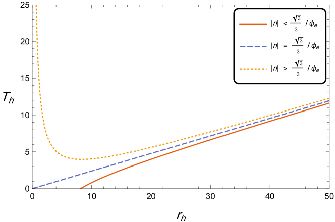
Figure 3.1: The temperature of the horizon of the black brane as a function of its horizon radius in case I.I for different values of $n$. The values used to draw this graph are ($l=1$, $\phi_{e}=15$, $\alpha=0$, $\widetilde{Q}_{m}=0$). The graph shows that for $n\leq\frac{\sqrt{3}}{3}l\phi_{e}$ the is only one possible black brane solution at any temperature, while for $n>\frac{\sqrt{3}}{3}l\phi_{e}$ there are two possible black brane solutions for $T_{h}\geq T_{min}$ and no possible solutions for $T_{h}<T_{min}.$

As shown in Fig.(3.1), if $\absolutevalue{n}\leq\frac{\sqrt{3}}{3}l\phi_{e}$, the temperature is a monotonic function of $r_{h}$, meaning that only one black brane can exist at any temperature. Also, there is always an extremal solution with a horizon radius $r_{e}$ given by

$$r_{e}=\frac{\sqrt{12\left(l^{2}\,\phi_{e}^{2}-3n^{2}\right)}}{6}.$$ (53)

However, if $\absolutevalue{n}>\frac{\sqrt{3}}{3}l\phi_{e}$, we see that the temperature has a minimum, $T_{min}$, at $r_{h}=r_{min}$ where

$$r_{min}=\frac{\sqrt{9n^{2}-3l^{2}\phi_{e}^{2}}}{3},$$ (54)

and

$$T_{min}\,=\frac{\sqrt{9n^{2}-3l^{2}\phi_{e}^{2}}}{2\pi l^{2}}.$$ (55)

It follows that at $T>T_{min}$ there are two possible black branes, a big black brane, and a small black brane. There is only one possible black brane at $T=T_{min}$. Finally, there are no possible black branes at $T<T_{min}$.

The Schwarzschild AdS solution [1] and some cases of the grand canonical ensemble of Reissner-Nordström AdS solution [4, 3] also have a minimum value for $T_{h}$. However, these cases always have a pure thermal solution that exists at any temperature which shares the same asymptotic metric as the black hole solutions. Our case lacks such a pure thermal solution. In fact, there is no known solution with the same asymptotic metric as the Taub-NUT dyonic AdS black brane metric. This means that in our case there are no known solutions that can exist at $T<T_{min}$. An educated guess would be that for $T<T_{min}$ the system will transit to a soliton-like solution, along the line that was presented in [42]. However, further investigation is required to confirm this assumption.

Using the same arguments as in the NUT-less case, we can see that the black brane is thermally stable when $\left(\frac{\partial{T}}{\partial{r_{h}}}\right)_{\phi_{e},\widetilde{Q}_{m},n}\geq 0$. In summary:

• For $\absolutevalue{n}>\frac{\sqrt{3}}{3}l\phi_{e}$ and $T<T_{min}$, there are no possible solutions.

• For $\absolutevalue{n}>\frac{\sqrt{3}}{3}l\phi_{e}$ and $T=T_{min}$, the only possible solution is one black brane solution, and it is thermally stable.

• For $\absolutevalue{n}>\frac{\sqrt{3}}{3}l\phi_{e}$ and $T>T_{min}$, there are two possible black brane solutions, the small black brane is thermally unstable while the big black brane is thermally stable.

• For $\absolutevalue{n}\leq\frac{\sqrt{3}}{3}l\phi_{e}$, the only possible solution is one black brane solution, and it is thermally stable.

Phase Diagram

To further investigate the different cases and the phases they contain, the grand potential density of the solution as a function of its horizon temperature is plotted for different values of $n$. This is shown n Fig. 3.2

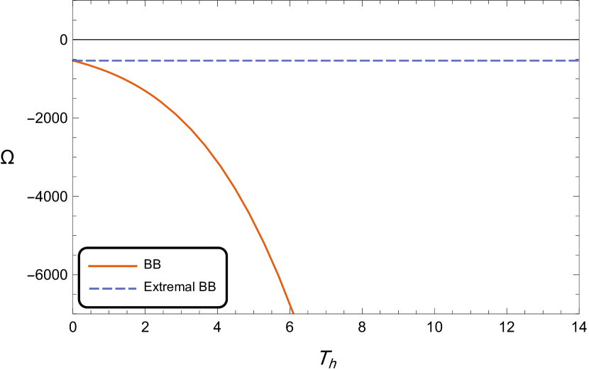
(a) $\absolutevalue{n}<\frac{\sqrt{3}}{3}l\phi_{e}$

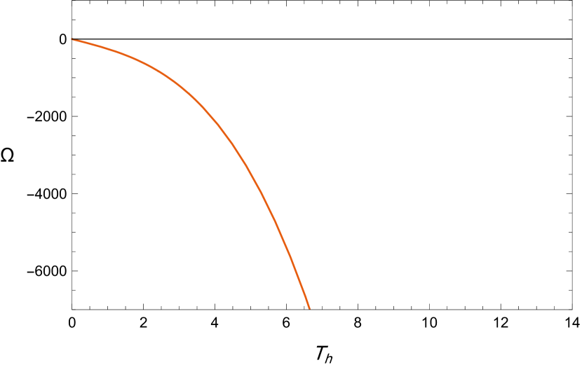
(b) $\absolutevalue{n}=\frac{\sqrt{3}}{3}l\phi_{e}$

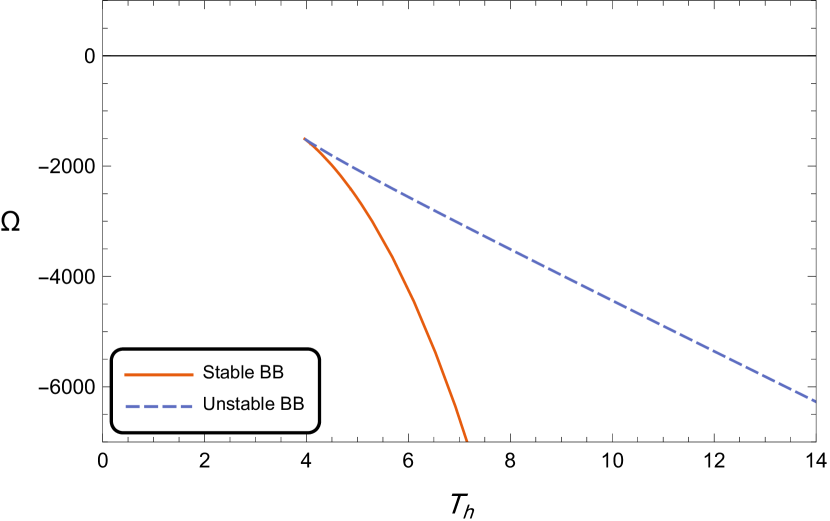
(c) $\absolutevalue{n}>\frac{\sqrt{3}}{3}l\phi_{e}$

Figure 3.2: The grand potential density of the black brane as a function of its horizon temperature in case I.I for different values of $n$. The values used to draw this graph are ($l=1$, $\phi_{e}=15$, $\alpha=0$, $\widetilde{Q}_{m}=0$). The graphs show that for $n\leq\frac{\sqrt{3}}{3}l\phi_{e}$ the grand potential of the black brane is always lower than that of the extremal black brane, while for $n>\frac{\sqrt{3}}{3}l\phi_{e}$ there is no extremal solution, and the stable black brane always have a lower grand potential than the unstable black brane.

From Fig. 3.2 we can see that for $\absolutevalue{n}<\frac{\sqrt{3}}{3}l\phi_{e}$ the non-extremal black brane always has a lower potential density than the extremal one, making it the thermodynamically preferable solution. For $\absolutevalue{n}>\frac{\sqrt{3}}{3}l\phi_{e}$ we can see the absence of an extremal solution. We can also see that no black brane can exist for $T<T_{min}$. On the other hand, for $T>T_{min}$ two black branes exist, with the thermally stable one always having a lower potential density than the non-stable one.

We are now fully acquainted with the required information to draw the $n-T$ phase diagram for this case. This is shown in Fig. 3.3. We can see from the figure that there is only one stable black brane everywhere except for the gray-shaded area where no black brane can exist.

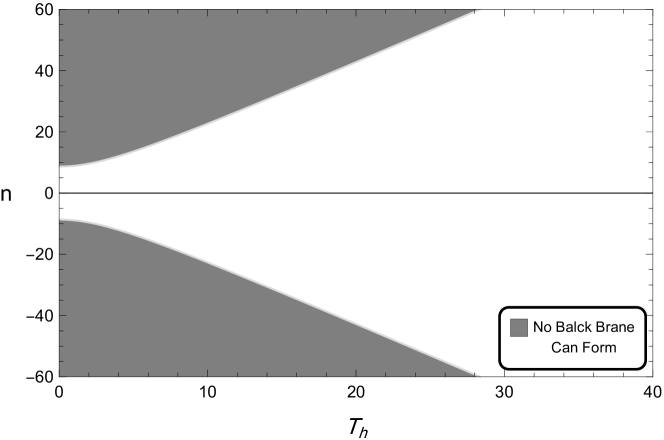
Figure 3.3: The $n-T$ phase diagram for case I.I. The values used to draw this graph are ($l=1$, $\phi_{e}=15$, $\alpha=0$, $\widetilde{Q}_{m}=0$). The graph shows that there exists only one phase everywhere except for the shaded gray area which marks where $T_{h}<T_{min}(n)$ and hence no black hole can exist in it.

Case I.II: $\widetilde{Q}_{m}\neq 0$

The non-vanishing magnetic charge density will make this case more interesting. The horizon temperature will take the form

$$T_{h}\,=\frac{3\left(r_{h}^{2}+n^{2}\right)}{4\pi l^{2}r_{h}}-\frac{\widetilde{Q}_{m}^{2}+r_{h}^{2}\phi_{e}^{2}}{4\pi r_{h}^{3}}.$$ (56)

Due to the non-vanishing $\widetilde{Q}_{m}$, an additional $-\frac{1}{r_{h}^{3}}$ term is present in the temperature formula. Fig. 3.4 shows that regardless the value of $n$, there always exists an extremal black brane with horizon radius $r_{e}$ given by

$$r_{e}=\frac{\sqrt{6\left(l^{2}\,\phi_{e}^{2}-3n^{2}\right)\,+\,6\,\sqrt{\left(l^{2}\,\phi_{e}^{2}-3n^{2}\right)^{2}\,+\,12l^{2}\widetilde{Q}_{m}^{2}}}}{6}.$$ (57)

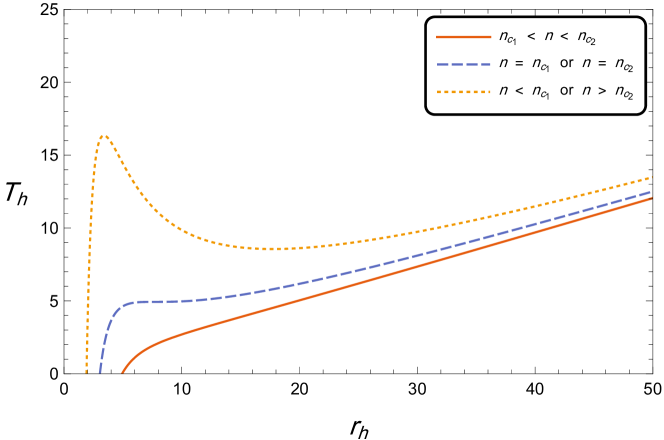
Figure 3.4: The temperature of the horizon of the black brane as a function of its horizon radius in case I.II for different values of $n$. Values used to draw this graph are ($l=1$, $\phi_{e}=15$, $\alpha=0$, $\widetilde{Q}_{m}=60$).

However, we either get three branches or one branch of the black brane solution depending on the value of $n$. We can also see that there are two critical values of $n$

$$n_{c_{1}}=-\frac{\sqrt{18l\widetilde{Q}_{m}+3l^{2}\phi_{e}^{2}}}{3},\quad n_{c_{2}}=\frac{\sqrt{18l\widetilde{Q}_{m}+3l^{2}\phi_{e}^{2}}}{3},$$ (58)

both corresponding to

$$r_{h(c)}=\sqrt{l\widetilde{Q}_{m}},$$ (59)

and

$$T_{c}=\frac{2\sqrt{l\widetilde{Q}_{m}}}{\pi l^{2}}.$$ (60)

For $n<n_{c_{1}}$ the horizon temperature of the black brane has a minimum value, $T_{min}$, at $r_{h}=r_{min}$ and a maximum value, $T_{max}$, at $r_{h}=r_{max}$. For $T<T_{min}$ or $T>T_{max}$ there exists only one black brane, while for $T\in(T_{min},T_{max})$ there exist three black branes. By increasing the value of $n$ the intervals $(T_{min},T_{max})$ and $(r_{min},r_{max})$ shrink until $n=n_{c_{1}}$, where $T_{min}$ and $T_{max}$ converge at $T_{c}$ and also $r_{min}$ and $r_{max}$ converge at $r_{h(c)}$. At this point, two branches of the black brane solution merge, while the third one disappears.

Increasing $n$ further, $T_{h}$ remains monotonic until $n=n_{c_{2}}$, after which the black brane solution re-splits into two branches while the third one reappears. The horizon temperature acquires minimum and maximum values again, with the intervals $(T_{min},T_{max})$ and $(r_{min},r_{max})$ keep widening as $n$ continues to increase.

From our previous discussion about the thermal stability of the black brane and from Fig. 3.4 we can then summarize the cases:

• For $n<n_{c_{1}}$ or $n>n_{c_{2}}$, and $T<T_{min}$ or $T>T_{max}$, the only possible solution is one black brane solution, and it is thermally stable.

• For $n<n_{c_{1}}$ or $n>n_{c_{2}}$, and $T\in(T_{min},T_{max})$, there are three possible black brane solutions, the small and the big black branes are thermally stable while the middle one is thermally unstable

• For $n<n_{c_{1}}$ or $n>n_{c_{2}}$, and $T=T_{min}$ or $T=T_{max}$, there are two possible black brane solutions, and both of them are thermally stable.

• For $n\in[n_{c_{1}},n_{c_{2}}]$, the only possible solution is one black brane solution, and it is thermally stable.

Phase Diagram

As before, we first plot the grand potential density of the solution as a function of its temperature, as it contains all the necessary information to explore the phase diagram of the solution. This is shown in Fig. 3.5.

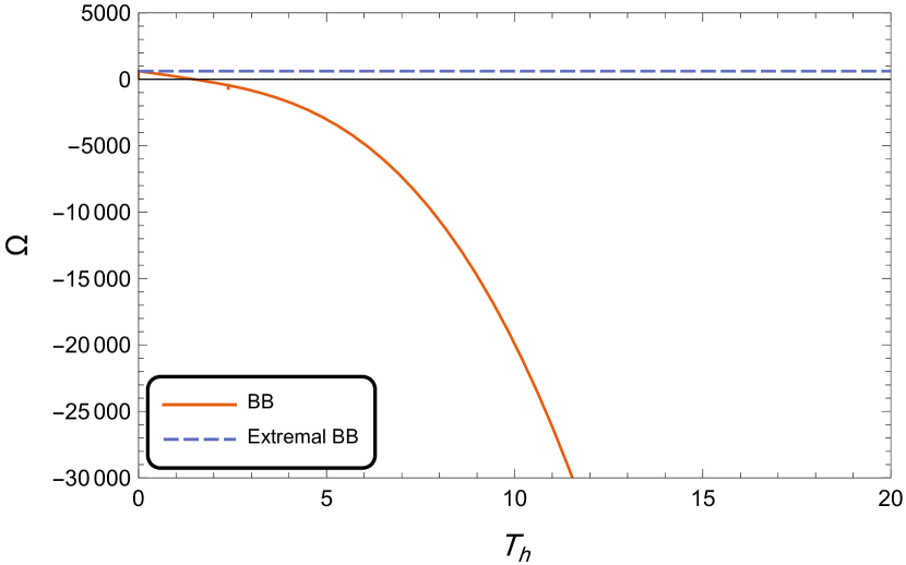
(a) $n_{c_{1}}<n<n_{c_{2}}$

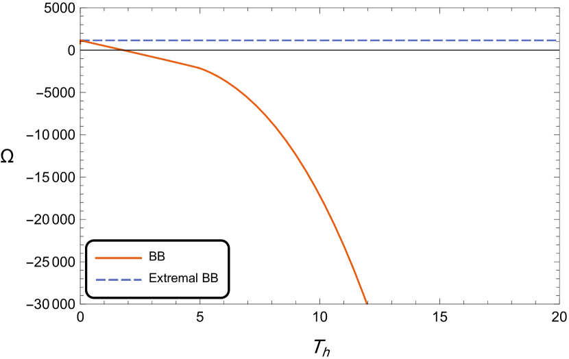
(b) $n=n_{c_{1}}$ or $n=n_{c_{2}}$

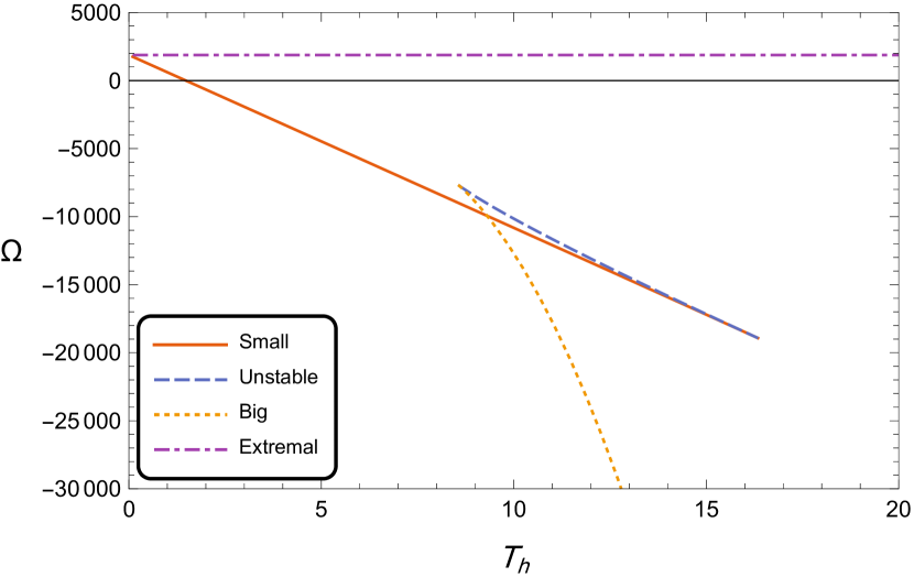
(c) $n<n_{c_{1}}$ or $n>n_{c_{2}}$

Figure 3.5: The grand potential density of the black brane as a function of its horizon temperature in case I.II for different values of $n$. The values used to draw this graph are ($l=1$, $\phi_{e}=15$, $\alpha=0$, $\widetilde{Q}_{m}=60$).

From Fig. 3.5, we can immediately notice the swallowtail behavior of the grand potential density for $n<n_{c_{1}}$ and $n>n_{c_{2}}$, signifying a first-order phase transition of the system. The grand potential densities of the small and the big black branes cross at $T=T_{tr}$, which marks a first-order phase transition between the two black branes. Also, we can notice that the unstable middle black brane is never thermodynamically preferred. Moreover, for any value of $n$ and non-zero temperatures, there is always a solution with grand potential density lower than the extremal black brane, meaning it is never thermodynamically preferred. Summarizing, we have

• For $n<n_{c_{1}}$ or $n>n_{c_{2}}$, and $T<T_{min}$ or $T>T_{max}$, the only stable solution is one black brane solution.

• For $n<n_{c_{1}}$ or $n>n_{c_{2}}$, and $T\in[T_{min},T_{tr})$, there are two stable black brane solutions, the small black brane is thermodynamically preferred while the big black brane is a metastable state.

• For $n<n_{c_{1}}$ or $n>n_{c_{2}}$, and $T=T_{tr}$, a first-order phase transition occurs between the small and the big black branes.

• For $n<n_{c_{1}}$ or $n>n_{c_{2}}$, and $T\in(T_{tr},T_{max}]$, there are two stable black brane solutions, the big black brane is thermodynamically preferred while the small black brane is a metastable state.

• For $n=n_{c_{1}}$ or $n=n_{c_{2}}$, and $T=T_{c}$, there is a critical point where the phase transition between the small and the big black branes vanishes and the two branes become indistinguishable.

• For $n\in[n_{c_{1}},n_{c_{2}}]$, the only stable solution is one black brane solution.

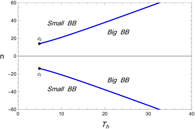
Figure 3.6: The $n-T$ phase diagram for case I.II. Values used to draw this graph are ($l=1$, $\phi_{e}=15$, $\alpha=0$, $\widetilde{Q}_{m}=60$).

From Fig. 3.6 and all the subsequent phase diagrams, we can see that no phase transitions or critical points exist along the line $n=0$ regardless of the values of the other thermodynamic quantities. This confirms that a non-zero NUT charge is the reason for these behaviors, as they disappear when $n$ vanishes. It is also important to stress that this is the first study to report first-order phase transitions and critical behavior when studying the regular thermodynamics of black holes with flat horizons without adding extra terms to the gravitational action.

3.2.2 Case II: $0<\absolutevalue{\alpha}\leq\frac{\sqrt{3}}{3}$

The non-vanishing $\alpha$ will make this case even more rich and understandably more complicated. With all of our thermodynamic quantities non-vanishing, the horizon temperature will take the general form in Eq.(51). Following the same approach, we divide this case into sub-cases depending on the value of $\widetilde{Q}_{m}$.

Case II.I: $\absolutevalue{\widetilde{Q}_{m}}<\frac{\alpha\,l\,\phi_{e}^{2}}{\sqrt{3}}$

This case is very close to case I.II in that regardless of the value of $n$ we always have an extremal solution with horizon radius $r_{e}$ given by

$$r_{e}=\frac{\sqrt{6\left(l^{2}\,\phi_{e}^{2}-3n^{2}\right)\,+\,6\,\sqrt{\left(l^{2}\,\phi_{e}^{2}-3n^{2}\right)^{2}\,+\,12l^{2}\left(\alpha n\phi_{e}-\widetilde{Q}_{m}\right)^{2}}}}{6},$$ (61)

and depending on the value of $n$ we either have one branch of the solution or three branches of the solution with two critical values of $n$,

$$n_{c_{1}}=-\frac{3\alpha^{2}l\phi_{e}^{2}+\sqrt{3\alpha^{2}l\phi_{e}^{2}\left(l\phi_{e}^{2}\,(3\alpha^{2}+1)+6\widetilde{Q}_{m}\right)}}{3\,\alpha\,\phi_{e}}$$

$$n_{c_{2}}=\frac{3\alpha^{2}l\phi_{e}^{2}+\sqrt{3\alpha^{2}l\phi_{e}^{2}\left(l\phi_{e}^{2}\,(3\alpha^{2}+1)-6\widetilde{Q}_{m}\right)}}{3\,\alpha\,\phi_{e}}$$ (62)

corresponding to

$$r_{h(c_{1})}=\frac{\sqrt{9\left(\alpha^{2}l^{2}\phi_{e}^{2}+l\widetilde{Q}_{m}\right)+3l\sqrt{3\alpha^{2}l\phi_{e}^{2}\left(l\phi_{e}^{2}\,(3\alpha^{2}+1)+6\widetilde{Q}_{m}\right)}}}{3},$$

$$r_{h(c_{2})}=\frac{\sqrt{9\left(\alpha^{2}l^{2}\phi_{e}^{2}-l\widetilde{Q}_{m}\right)+3l\sqrt{3\alpha^{2}l\phi_{e}^{2}\left(l\phi_{e}^{2}\,(3\alpha^{2}+1)-6\widetilde{Q}_{m}\right)}}}{3},$$ (63)

and

$$T_{c_{1}}=\frac{2}{3\pi l^{2}}\sqrt{9\left(\alpha^{2}l^{2}\phi_{e}^{2}+l\widetilde{Q}_{m}\right)+3l\sqrt{3\alpha^{2}l\phi_{e}^{2}\left(l\phi_{e}^{2}\,(3\alpha^{2}+1)+6\widetilde{Q}_{m}\right)}},$$

$$T_{c_{2}}=\frac{2}{3\pi l^{2}}\sqrt{9\left(\alpha^{2}l^{2}\phi_{e}^{2}-l\widetilde{Q}_{m}\right)+3l\sqrt{3\alpha^{2}l\phi_{e}^{2}\left(l\phi_{e}^{2}\,(3\alpha^{2}+1)-6\widetilde{Q}_{m}\right)}}.$$ (64)

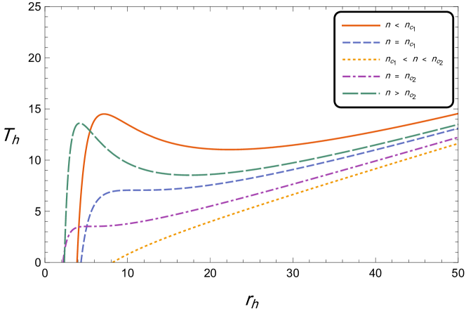
Figure 3.7: The temperature of the horizon of the black brane as a function of its horizon radius in case II.I for different values of $n$. Values used to draw this graph are ($l=1$, $\phi_{e}=15$, $\alpha=\frac{\sqrt{3}}{5}$, $\widetilde{Q}_{m}=30$).

However, as we can see from Fig. 3.7, unlike case I.II, $n_{c_{1}}\neq-n_{c_{2}}$, $r_{h(c_{1})}\neq r_{h(c_{2})}$, and $T_{c_{1}}\neq T_{c_{2}}$, except for the special case when $\widetilde{Q}_{m}=0$, making the $n-T$ phase diagram, Fig.(3.8), not symmetric in general under $n\longrightarrow-n$ except for $\widetilde{Q}_{m}=0$ as we mentioned.

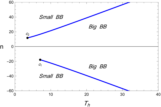
Figure 3.8: The $n-T$ phase diagram for case II.I. Values used to draw this graph are ($l=1$, $\phi_{e}=15$,$\alpha=\frac{\sqrt{3}}{5}$, $\widetilde{Q}_{m}=30$).

Varying $\absolutevalue{\widetilde{Q}_{m}}$ within the range $[0,\frac{\alpha\,l\,\phi_{e}^{2}}{\sqrt{3}})$ does not change the characteristics of the phase diagram but affects its shape. Decreasing $\absolutevalue{\widetilde{Q}_{m}}$ shrinks the interval $[T_{c_{1}},T_{c_{2}}]$ until $T_{c_{1}}=T_{c_{2}}$ at $\widetilde{Q}_{m}=0$. On the other hand, increasing $\absolutevalue{\widetilde{Q}_{m}}$ widens the interval $[T_{c_{1}},T_{c_{2}}]$ with $T_{c_{2}}\longrightarrow 0$ as $\absolutevalue{\widetilde{Q}_{m}}\longrightarrow\frac{\alpha\,l\,\phi_{e}^{2}}{\sqrt{3}}$.

Case II.II: $\absolutevalue{\widetilde{Q}_{m}}=\frac{\alpha\,l\,\phi_{e}^{2}}{\sqrt{3}}$

Substituting the value $\widetilde{Q}_{m}=\frac{\alpha\,l\,\phi_{e}^{2}}{\sqrt{3}}$ in the general formula of $T_{h}$ in Eq.(51) we get

$$T_{h}\,=\frac{3\left(r_{h}^{2}+n^{2}\right)}{4\pi l^{2}r_{h}}-\frac{3r_{h}^{2}\phi_{e}^{2}+\alpha^{2}\phi_{e}^{2}\left(\,l\,\phi_{e}-\sqrt{3}n\right)^{2}}{12\pi r^{3}_{h}}.$$ (65)

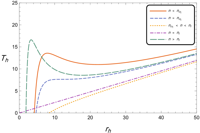
Figure 3.9: The temperature of the horizon of the black brane as a function of its horizon radius in case II.II for different values of $n$. The values used to draw this graph are ($l=1$, $\phi_{e}=15$, $\alpha=\frac{\sqrt{3}}{5}$, $\widetilde{Q}_{m}=45$).

Comparing this case with the previous one, we find that $n_{c_{1}}$ is the only critical point with

$$n_{c}=\alpha^{2}l^{2}\phi_{e}^{3}\left(\sqrt{3}+3\alpha\right)$$ (66)

corresponding to

$$r_{h(c)}=\frac{l\phi_{e}\sqrt{6\alpha\left(3\alpha+\sqrt{3}\right)}}{3},$$ (67)

and

$$T_{c}=\frac{2\phi_{e}\sqrt{6\alpha\left(3\alpha+\sqrt{3}\right)}}{3\pi l},$$

$n_{c_{2}}$ is no longer a critical point. However, it still separates between a three-branched solution and a one-branched solution for $T_{h}(r_{h})$. We will call it $n_{l}$, where

$$n_{l}=\alpha^{2}l^{2}\phi_{e}^{3}\left(\sqrt{3}-3\alpha\right)$$ (68)

The reason $n_{l}$ is not a critical value of $n$ is that, as we can see from Fig. 3.9, at $n=n_{l}$, the $T_{h}-r_{h}$ curve doesn’t have a saddle point. Instead, the horizon temperature of the black brane becomes a linear function of its horizon radius, $T_{h}=\frac{3r_{h}}{4\pi}$. That results in one of the phases being disjointed from the rest of the phases as seen in the phase diagram in Fig. 3.10.

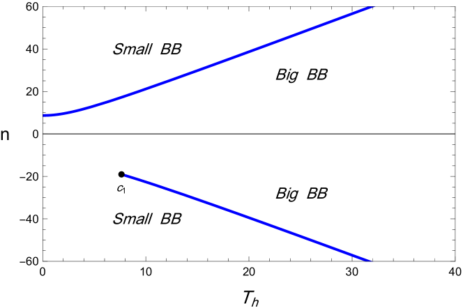
Figure 3.10: The $n-T$ phase diagram for case II.II. The values used to draw this graph are ($l=1$, $\phi_{e}=15$, $\alpha=\frac{\sqrt{3}}{5}$, $\widetilde{Q}_{m}=45$).

Case II.III: $\absolutevalue{\widetilde{Q}_{m}}>\frac{\alpha\,l\,\phi_{e}^{2}}{\sqrt{3}}$

This case is very similar to the canonical ensemble of Reissner-Nordström-anti-de Sitter (RNAdS) black hole [4, 3].

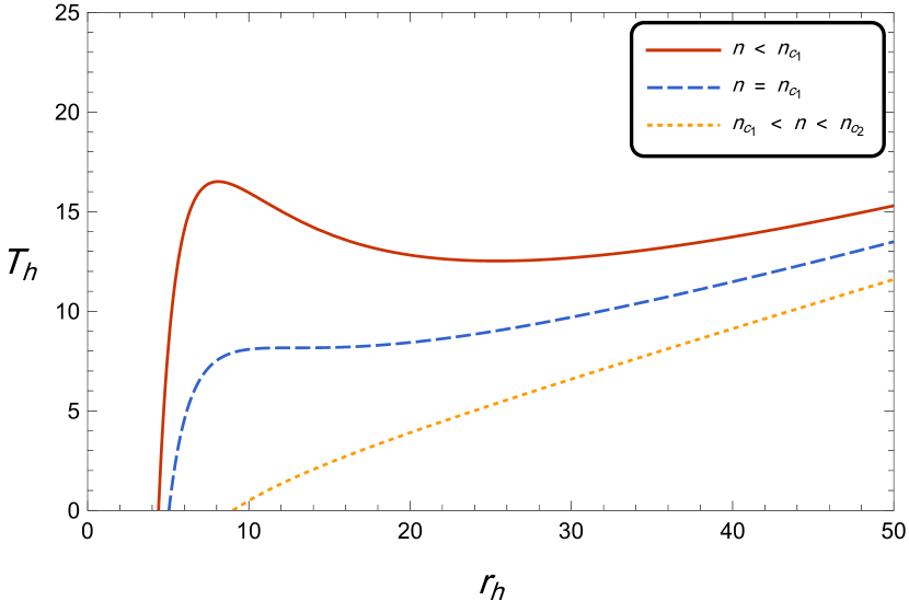
(a) $-\infty<n<n_{c_{2}}$

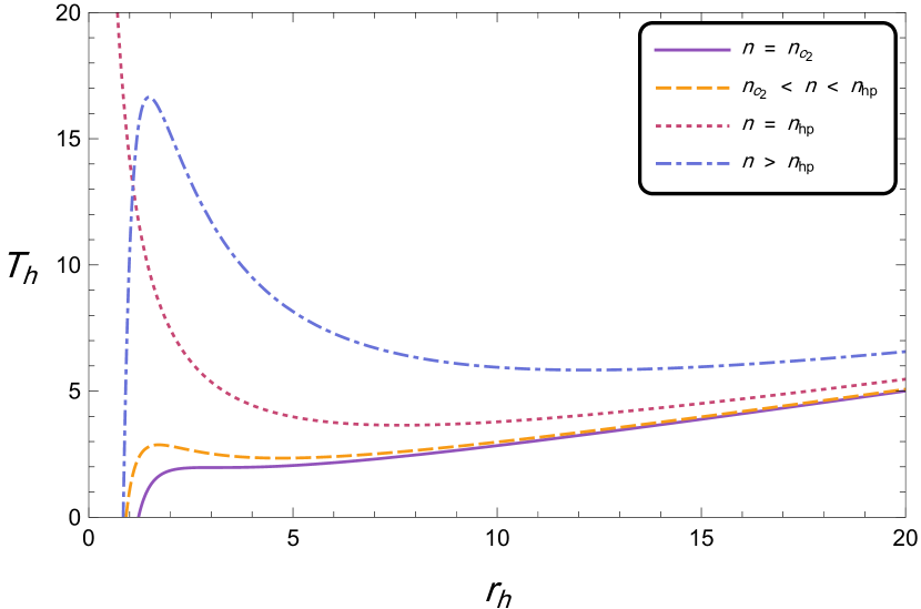
(b) $n_{c_{2}}\leq n<\infty$

Figure 3.11: The temperature of the horizon of the black brane as a function of its horizon radius in case II.III for different values of $n$. The values used to draw this graph are ($l=1$, $\phi_{e}=15$, $\alpha=\frac{\sqrt{3}}{5}$, $\widetilde{Q}_{m}=60$). Here we split the graph into two for clarity.

Similar to the previous case, we find two critical values for $n$,

$$n_{c_{1}}=-\frac{3\alpha^{2}l\phi_{e}^{2}+\sqrt{3\alpha^{2}l\phi_{e}^{2}\left(l\phi_{e}^{2}\,(3\alpha^{2}+1)+6\widetilde{Q}_{m}\right)}}{3\,\alpha\,\phi_{e}}$$

$$n_{c_{2}}=\frac{-3\alpha^{2}l\phi_{e}^{2}+\sqrt{3\alpha^{2}l\phi_{e}^{2}\left(l\phi_{e}^{2}\,(3\alpha^{2}+1)+6\widetilde{Q}_{m}\right)}}{3\,\alpha\,\phi_{e}},$$ (69)

corresponding to

$$r_{h(c_{1})}=\frac{\sqrt{9\left(\alpha^{2}l^{2}\phi_{e}^{2}+l\widetilde{Q}_{m}\right)+3l\sqrt{3\alpha^{2}l\phi_{e}^{2}\left(l\phi_{e}^{2}\,(3\alpha^{2}+1)+6\widetilde{Q}_{m}\right)}}}{3},$$

$$r_{h(c_{2})}=\frac{\sqrt{9\left(\alpha^{2}l^{2}\phi_{e}^{2}+l\widetilde{Q}_{m}\right)-3l\sqrt{3\alpha^{2}l\phi_{e}^{2}\left(l\phi_{e}^{2}\,(3\alpha^{2}+1)+6\widetilde{Q}_{m}\right)}}}{3},$$ (70)

and

$$T_{c_{1}}=\frac{2}{3\pi l^{2}}\sqrt{9\left(\alpha^{2}l^{2}\phi_{e}^{2}+l\widetilde{Q}_{m}\right)+3l\sqrt{3\alpha^{2}l\phi_{e}^{2}\left(l\phi_{e}^{2}\,(3\alpha^{2}+1)+6\widetilde{Q}_{m}\right)}},$$

$$T_{c_{2}}=\frac{2}{3\pi l^{2}}\sqrt{9\left(\alpha^{2}l^{2}\phi_{e}^{2}+l\widetilde{Q}_{m}\right)-3l\sqrt{3\alpha^{2}l\phi_{e}^{2}\left(l\phi_{e}^{2}\,(3\alpha^{2}+1)+6\widetilde{Q}_{m}\right)}},$$ (71)

with $T_{h}(r_{h})$ has one black brane branch for $n\in[n_{c_{1}},n_{c_{2}}]$ and three branches for $n<n_{c_{1}}$ or $n>n_{c_{2}}$, except when $n=\frac{\widetilde{Q}_{m}}{\alpha\phi_{e}}$. We will give this value of $n$ a special name, $n_{hp}$, where hp stands for Hawking-Page. The reason for this is that for $n=n_{hp}$ the solution behaves exactly like a Schwarzschild anti-de Sitter solution described in [1]. At this value of $n$, the horizon temperature has a minimum value $T_{min}$;

$$T_{min}\,=\frac{\sqrt{9\widetilde{Q}_{m}^{2}-3\alpha^{3}l^{2}\phi_{e}^{4}}}{2\pi\alpha\phi_{e}l^{2}}.$$ (72)

with

$$r_{min}=\frac{\sqrt{9\widetilde{Q}_{m}^{2}-3\alpha^{3}l^{2}\phi_{e}^{4}}}{3\alpha\phi_{e}},$$ (73)

For $T>T_{min}$, one thermally stable and one thermally unstable black brane exist. For $T=T_{min}$, one thermally stable black brane exists, and no black branes exist for $T<T_{min}$. In fact, as we discussed in case I.I, no known solution can exist at this range of temperatures. To check the thermal preferability of the phases, we plot $\Omega(T_{h})$, Fig 3.13.

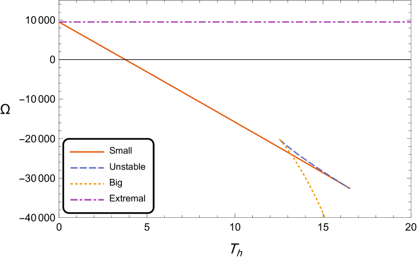
(a) $n<n_{c_{1}}$

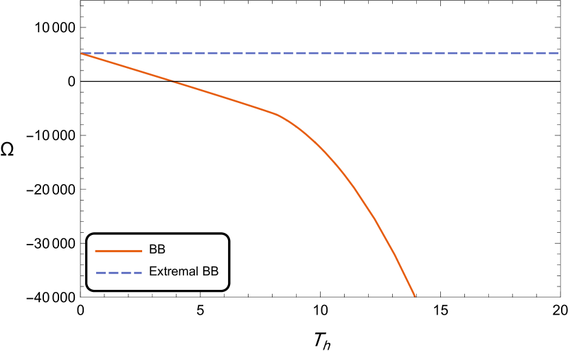
(b) $n=n_{c_{1}}$

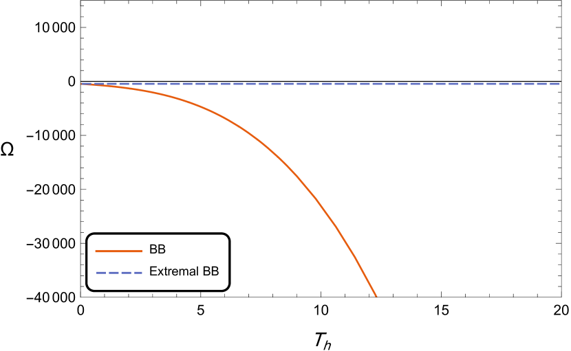
(c) $n_{c_{1}}<n<n_{c_{2}}$

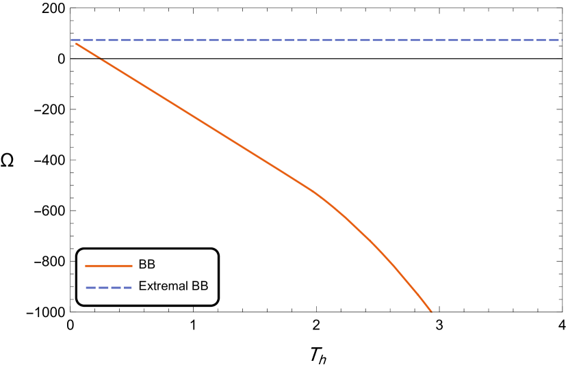
(d) $n=n_{c_{2}}$

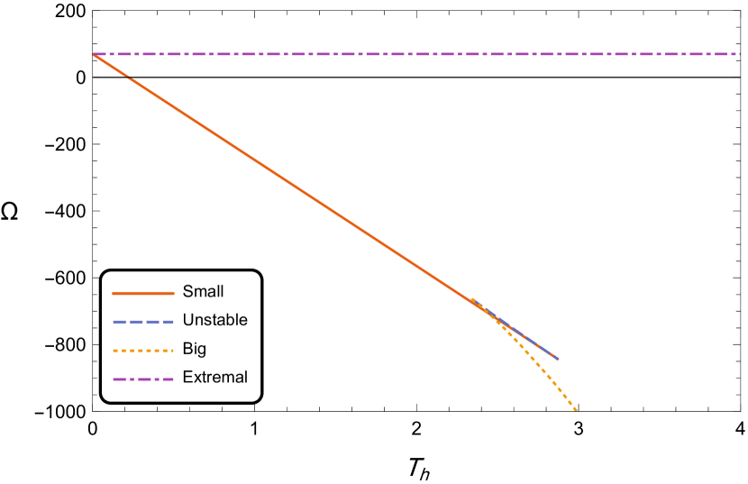
(e) $n_{c_{2}}<n<n_{hp}$

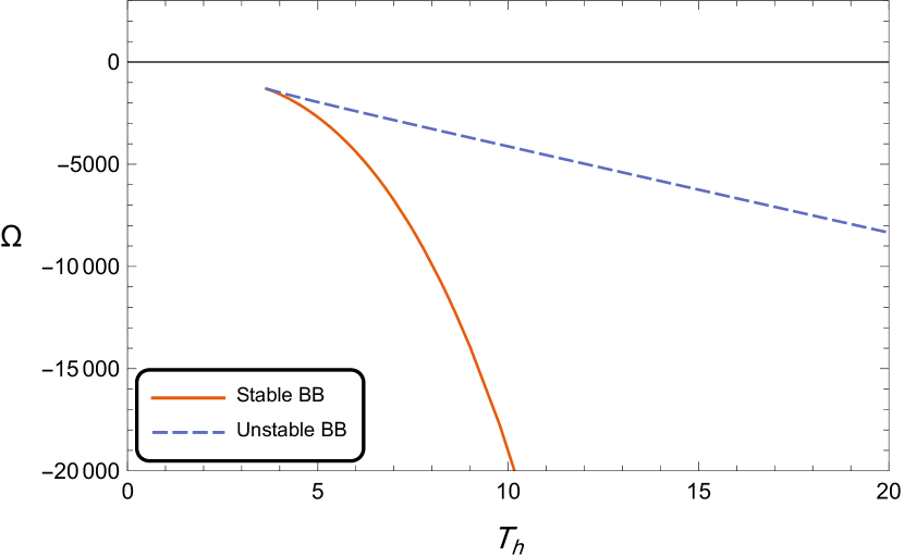
(f) $n=n_{hp}$

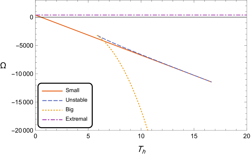
(a) $n>n_{hp}$

Figure 3.13: The grand potential density of the black brane as a function of its horizon temperature in case II.III for different values of $n$. The values used to draw this graph are ($l=1$, $\phi_{e}=15$, $\alpha=\frac{\sqrt{3}}{5}$, $\widetilde{Q}_{m}=60$).

Summarizing our results, we have:

• For $\,n<n_{c_{1}}$, $\;n\in(n_{c_{2}},n_{hp})$, or $\;n>n_{hp}\,$ and $\,T<T_{min}$ or $T>T_{max}\,$, the only stable solution is one black brane solution.

• For $\,n<n_{c_{1}}$, $\;n\in(n_{c_{2}},n_{hp})$, or $\;n>n_{hp}\,$ and $T\in[T_{min},T_{tr})$, there are two stable black brane solutions. The small black brane is thermodynamically preferred, while the big black brane is a metastable state.

• For $\,n<n_{c_{1}}$, $\;n\in(n_{c_{2}},n_{hp})$, or $\;n>n_{hp}\,$ and $T=T_{tr}$, first-order phase transition occurs between the small and the big black branes.

• For $\,n<n_{c_{1}}$, $\;n\in(n_{c_{2}},n_{hp})$, or $\;n>n_{hp}\,$ and $T\in(T_{tr},T_{max}]$, there are two stable black brane solutions. The big black brane is thermodynamically preferred while the small black brane is a metastable state.

• For $n=n_{c_{1}}$ and $T=T_{c_{1}}$ or $n=n_{c_{2}}$ and $T=T_{c_{2}}$, there is a critical point where the first-order phase transition between the small and the big black branes ends, and the two branes become indistinguishable.

• For $n\in[n_{c_{1}},n_{c_{2}}]$, the only stable solution is one black brane solution.

• For $n=n_{hp}$ and $T<T_{min}$, there are no possible solutions.

• For $n=n_{hp}$ and $T\geq T_{min}$, the only stable solution is a one black brane solution.

The complete phase diagram is shown in Fig 3.14.

(a)

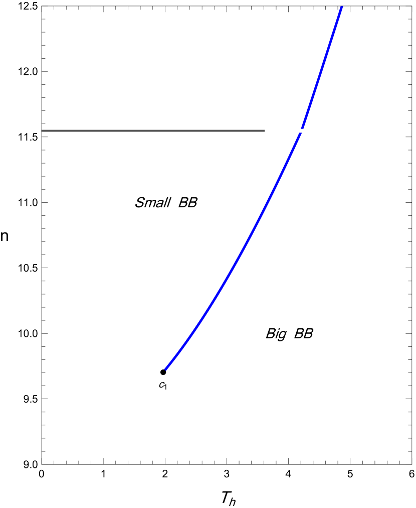
(b)

Figure 3.14: The $n-T$ phase diagram for case II.III. The values used to draw this graph are ($l=1$, $\phi_{e}=15$, $\alpha=\frac{\sqrt{3}}{5}$, $\widetilde{Q}_{m}=60$). The gray line at $n=n_{hp}$ shows the region where no black brane can exist.

3.2.3 Case III: $\absolutevalue{\alpha}>\frac{\sqrt{3}}{3}$

Similar to Case II, there are no vanishing thermodynamic quantities, so the temperature of the black brane takes the general form in Eq.(51). Results now depend on the value of $\widetilde{Q}_{m}$.

Case III.I: $\widetilde{Q}_{m}\in[-\frac{\alpha\,l\,\phi_{e}^{2}}{\sqrt{3}},\frac{\alpha\,l\,\phi_{e}^{2}}{\sqrt{3}}]$

This case is exactly the same as Case II.I

Case III.II: $\widetilde{Q}_{m}\in[-\frac{l\phi_{e}^{2}\left(1+3\alpha^{2}\right)}{6},-\frac{\alpha\,l\,\phi_{e}^{2}}{\sqrt{3}})$ or $\widetilde{Q}_{m}\in(\frac{\alpha\,l\,\phi_{e}^{2}}{\sqrt{3}},\frac{l\phi_{e}^{2}\left(1+3\alpha^{2}\right)}{6}]$

As stated earlier, the number of branches of the $T_{h}(r_{h})$ solution varies due to the value of $n$. In this case, there are four critical values of $n$,

$$n_{c_{1}}=-\frac{3\alpha^{2}l\phi_{e}^{2}+\sqrt{3\alpha^{2}l\phi_{e}^{2}\left(l\phi_{e}^{2}\,(3\alpha^{2}+1)+6\widetilde{Q}_{m}\right)}}{3\,\alpha\,\phi_{e}},$$

$$n_{c_{2}}=\frac{-3\alpha^{2}l\phi_{e}^{2}+\sqrt{3\alpha^{2}l\phi_{e}^{2}\left(l\phi_{e}^{2}\,(3\alpha^{2}+1)+6\widetilde{Q}_{m}\right)}}{3\,\alpha\,\phi_{e}},$$

$$n_{c_{3}}=\frac{3\alpha^{2}l\phi_{e}^{2}-\sqrt{3\alpha^{2}l\phi_{e}^{2}\left(l\phi_{e}^{2}\,(3\alpha^{2}+1)-6\widetilde{Q}_{m}\right)}}{3\,\alpha\,\phi_{e}},$$

$$n_{c_{4}}=\frac{3\alpha^{2}l\phi_{e}^{2}+\sqrt{3\alpha^{2}l\phi_{e}^{2}\left(l\phi_{e}^{2}\,(3\alpha^{2}+1)-6\widetilde{Q}_{m}\right)}}{3\,\alpha\,\phi_{e}}.$$ (74)

corresponding to

$$r_{h(c_{1})}=\frac{\sqrt{9\left(\alpha^{2}l^{2}\phi_{e}^{2}+l\widetilde{Q}_{m}\right)+3l\sqrt{3\alpha^{2}l\phi_{e}^{2}\left(l\phi_{e}^{2}\,(3\alpha^{2}+1)+6\widetilde{Q}_{m}\right)}}}{3},$$

$$r_{h(c_{2})}=\frac{\sqrt{9\left(\alpha^{2}l^{2}\phi_{e}^{2}+l\widetilde{Q}_{m}\right)-3l\sqrt{3\alpha^{2}l\phi_{e}^{2}\left(l\phi_{e}^{2}\,(3\alpha^{2}+1)+6\widetilde{Q}_{m}\right)}}}{3},$$

$$r_{h(c_{3})}=\frac{\sqrt{9\left(\alpha^{2}l^{2}\phi_{e}^{2}-l\widetilde{Q}_{m}\right)-3l\sqrt{3\alpha^{2}l\phi_{e}^{2}\left(l\phi_{e}^{2}\,(3\alpha^{2}+1)-6\widetilde{Q}_{m}\right)}}}{3},$$

$$r_{h(c_{4})}=\frac{\sqrt{9\left(\alpha^{2}l^{2}\phi_{e}^{2}-l\widetilde{Q}_{m}\right)+3l\sqrt{3\alpha^{2}l\phi_{e}^{2}\left(l\phi_{e}^{2}\,(3\alpha^{2}+1)-6\widetilde{Q}_{m}\right)}}}{3}.$$ (75)

and

$$T_{c_{1}}=\frac{2}{3\pi l^{2}}\sqrt{9\left(\alpha^{2}l^{2}\phi_{e}^{2}+l\widetilde{Q}_{m}\right)+3l\sqrt{3\alpha^{2}l\phi_{e}^{2}\left(l\phi_{e}^{2}\,(3\alpha^{2}+1)+6\widetilde{Q}_{m}\right)}},$$

$$T_{c_{2}}=\frac{2}{3\pi l^{2}}\sqrt{9\left(\alpha^{2}l^{2}\phi_{e}^{2}+l\widetilde{Q}_{m}\right)-3l\sqrt{3\alpha^{2}l\phi_{e}^{2}\left(l\phi_{e}^{2}\,(3\alpha^{2}+1)+6\widetilde{Q}_{m}\right)}},$$

$$T_{c_{3}}=\frac{2}{3\pi l^{2}}\sqrt{9\left(\alpha^{2}l^{2}\phi_{e}^{2}-l\widetilde{Q}_{m}\right)-3l\sqrt{3\alpha^{2}l\phi_{e}^{2}\left(l\phi_{e}^{2}\,(3\alpha^{2}+1)-6\widetilde{Q}_{m}\right)}},$$

$$T_{c_{4}}=\frac{2}{3\pi l^{2}}\sqrt{9\left(\alpha^{2}l^{2}\phi_{e}^{2}-l\widetilde{Q}_{m}\right)+3l\sqrt{3\alpha^{2}l\phi_{e}^{2}\left(l\phi_{e}^{2}\,(3\alpha^{2}+1)-6\widetilde{Q}_{m}\right)}}.$$ (76)

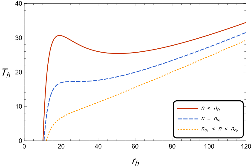
(a) $-\infty<n<n_{c_{2}}$

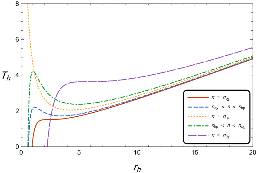
(b) $n_{c_{2}}\leq n\leq n_{c_{3}}$

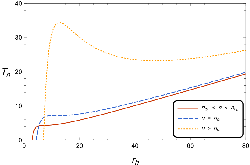
(c) $n_{c_{3}}<n<\infty$

Figure 3.15: The temperature of the horizon of the black brane as a function of its horizon radius in case III.II for different values of $n$. The values used to draw this graph are ($l=1$, $\phi_{e}=15$, $\alpha=1$, $\widetilde{Q}_{m}=145$). Here we split the graph into three for clarity.

From Fig. 3.15 we can see that for $n\in[n_{c_{1}},n_{c_{2}}]$ or $n\in[n_{c_{3}},n_{c_{4}}]$ the horizon temperature of the black brane, $T_{h}(r_{h})$, has only one branch. For $n<n_{c_{1}}$ or $n>n_{c_{4}}$, it has three branches. Finally, for $n\in(n_{c_{2}},n_{c_{3}})$, it also has three branches except for $n=n_{hp}=\frac{\widetilde{Q}_{m}}{\alpha\phi_{e}}$ where $T_{h}(r_{h})$ has two branches and a minimum value at $r_{h}=r_{min}$ given by Eq.(73) which corresponds to $T_{min}$ given by Eq.(72).

Following the same procedure as in the previous cases, we next check the thermal preferability of the phases by plotting $\Omega(T_{h})$, Fig. 3.17.

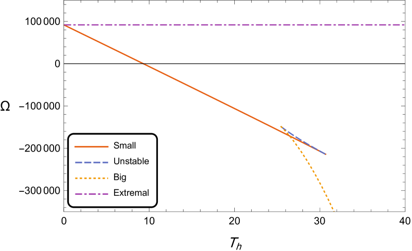
(a) $n<n_{c_{1}}$

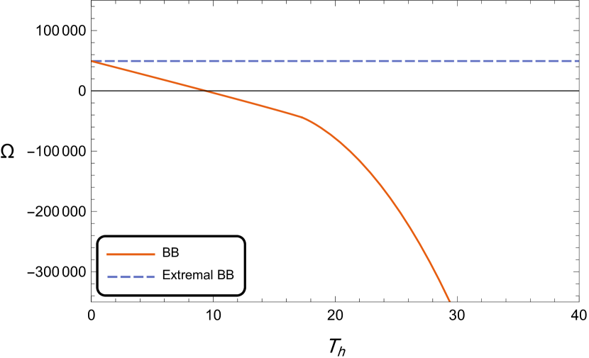
(b) $n=n_{c_{1}}$

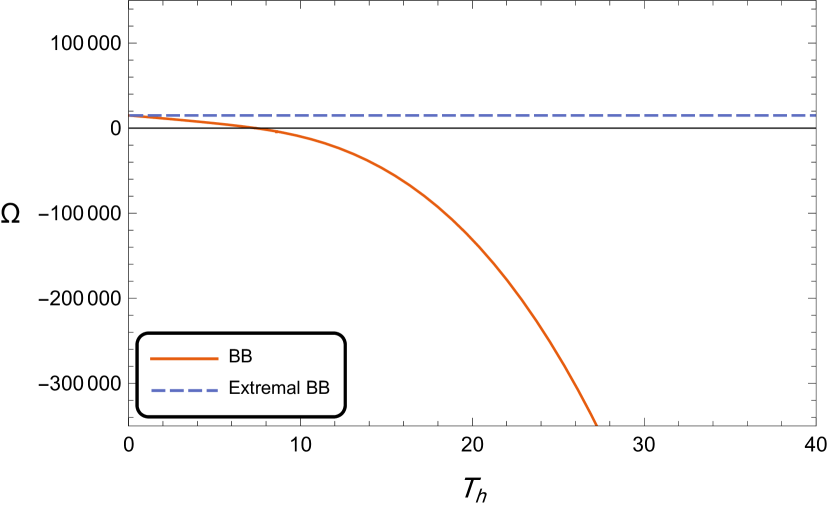
(c) $n_{c_{1}}<n<n_{c_{2}}$

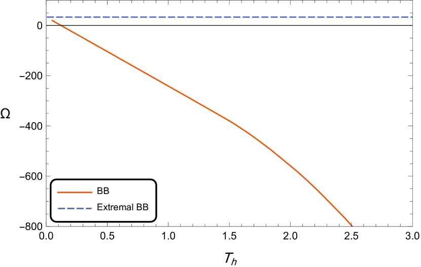
(d) $n=n_{c_{2}}$

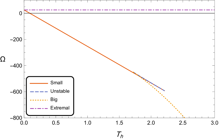
(e) $n_{c_{2}}<n<n_{hp}$

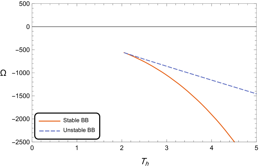
(f) $n=n_{hp}$

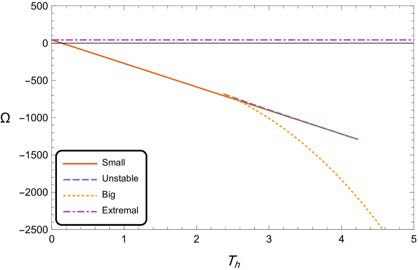
(a) $n_{hp}<n<n_{c_{3}}$

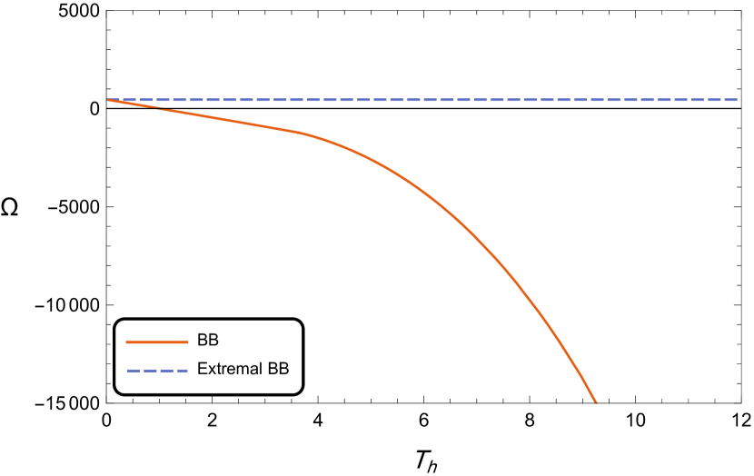
(b) $n=n_{c_{3}}$

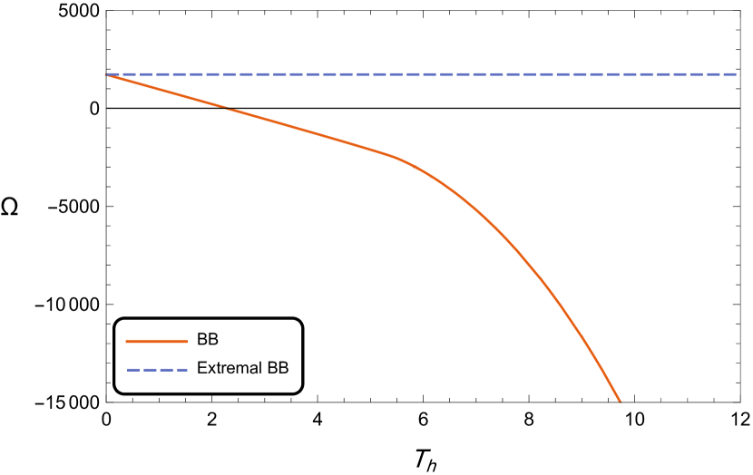
(c) $n_{c_{3}}<n<n_{c_{4}}$

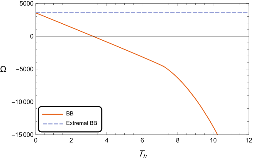
(d) $n=n_{c_{4}}$

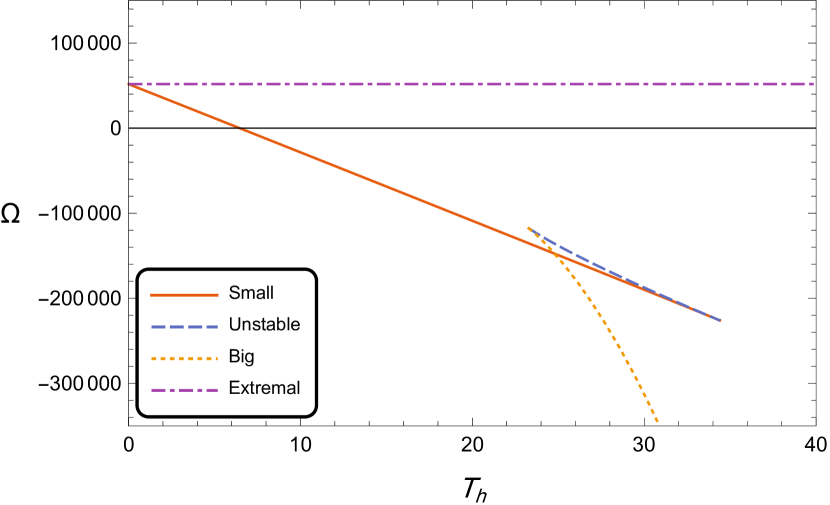
(e) $n>n_{c_{4}}$

Figure 3.17: The grand potential density of the black brane as a function of its horizon temperature in case III.II for different values of $n$. The values used to draw this graph are ($l=1$, $\phi_{e}=15$, $\alpha=1$, $\widetilde{Q}_{m}=145$).

In summary, we have

• For $\,n<n_{c_{1}}$, $\;n\in(n_{c_{2}},n_{hp})$, $\;n\in(n_{hp},n_{c_{3}})$, or $\;n>n_{c_{4}}\,$ and $\,T<T_{min}$ or $T>T_{max}\,$, the only stable solution is one black brane solution.

• For $\,n<n_{c_{1}}$, $\;n\in(n_{c_{2}},n_{hp})$, $\;n\in(n_{hp},n_{c_{3}})$, or $\;n>n_{c_{4}}\,$ and $T\in[T_{min},T_{tr})$, there are two stable black brane solutions, the small black brane is thermodynamically preferred while the big black brane is a metastable state.

• For $\,n<n_{c_{1}}$, $\;n\in(n_{c_{2}},n_{hp})$, $\;n\in(n_{hp},n_{c_{3}})$, or $\;n>n_{c_{4}}\,$ and $T=T_{tr}$, first-order phase transition occurs between the small and the big black branes.

• For $\,n<n_{c_{1}}$, $\;n\in(n_{c_{2}},n_{hp})$, $\;n\in(n_{hp},n_{c_{3}})$, or $\;n>n_{c_{4}}\,$ and $T\in(T_{tr},T_{max}]$, there are two stable black brane solutions, the big black brane is thermodynamically preferred while the small black brane is a metastable state.

• For $n=n_{c_{1}}$ and $T=T_{c_{1}}$, $n=n_{c_{2}}$ and $T=T_{c_{2}}$, $n=n_{c_{3}}$ and $T=T_{c_{3}}$ or $n=n_{c_{4}}$ and $T=T_{c_{4}}$, there is a critical point where the first-order phase transition between the small and the big black branes ends, and the two branes become indistinguishable.

• For $n\in[n_{c_{1}},n_{c_{2}}]$ or $n\in[n_{c_{3}},n_{c_{4}}]$, the only stable solution is one black brane solution.

• For $n=n_{hp}$ and $T<T_{min}$, there are no possible solutions.

• For $n=n_{hp}$ and $T\geq T_{min}$, the only stable solution is one black brane solution.

The complete phase diagram for this case is shown in Fig. 3.18

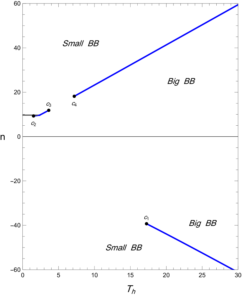
(a)

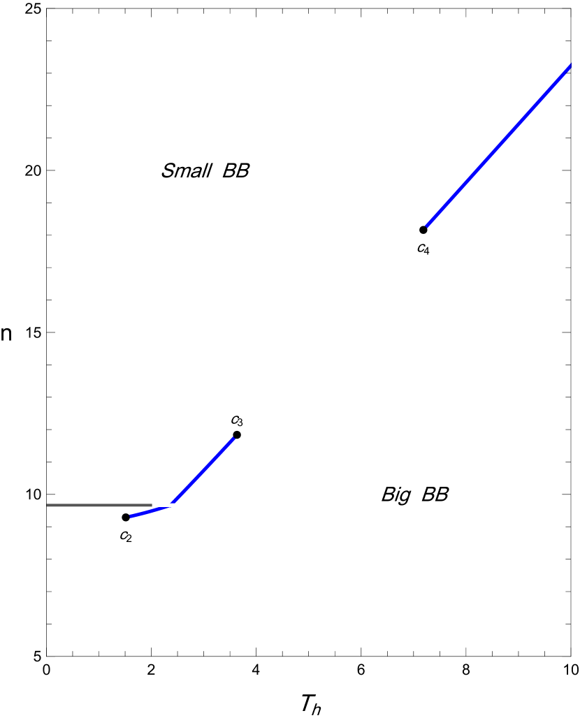
(b)

Figure 3.18: The $n-T$ phase diagram for case III.II. The values used to draw this graph are ($l=1$, $\phi_{e}=15$, $\alpha=1$, $\widetilde{Q}_{m}=145$). The gray line at $n=n_{hp}$ shows the region where no black brane can exist.

As the value of $\widetilde{Q}_{m}$ increases in the region $(\frac{\alpha\,l\,\phi_{e}^{2}}{\sqrt{3}},\frac{l\phi_{e}^{2}\left(1+3\alpha^{2}\right)}{6}]$, the intervals $(n_{c_{2}},n_{c_{3}})$ and $(T_{c_{2}},T_{c_{3}})$ shrink until the two critical points merge at $\widetilde{Q}_{m}=\frac{l\phi_{e}^{2}\left(1+3\alpha^{2}\right)}{6}$. This can be seen from the phase diagram in Fig. 3.19.

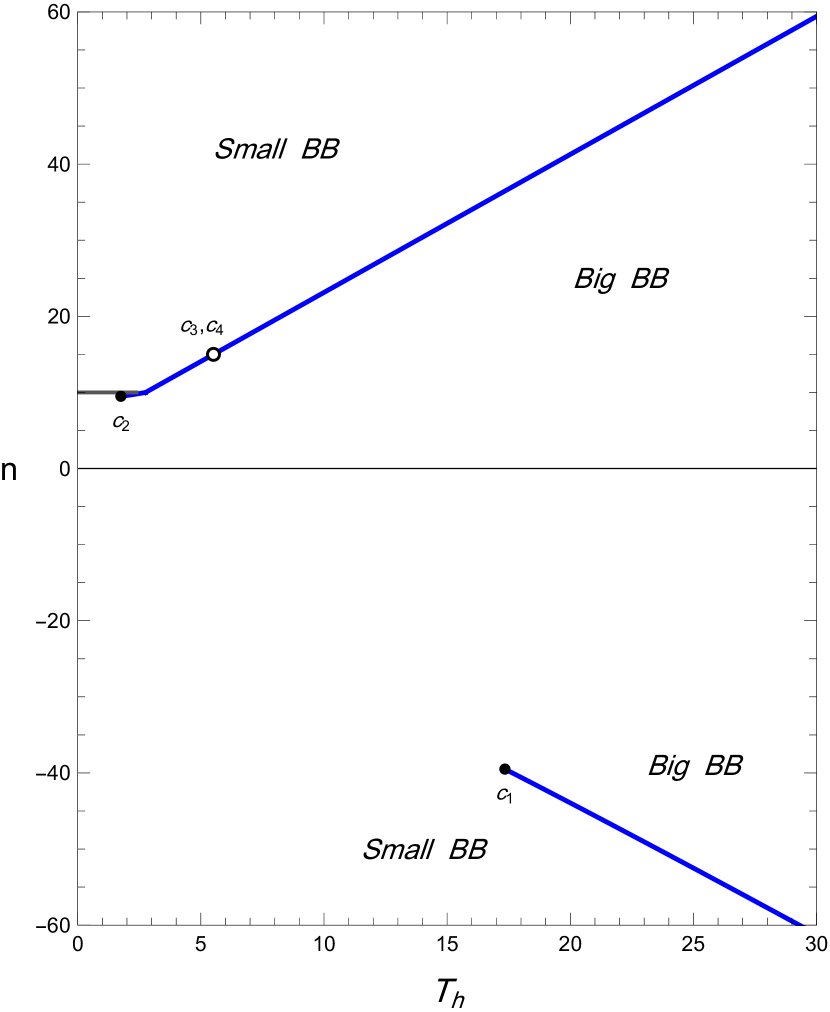
(a)

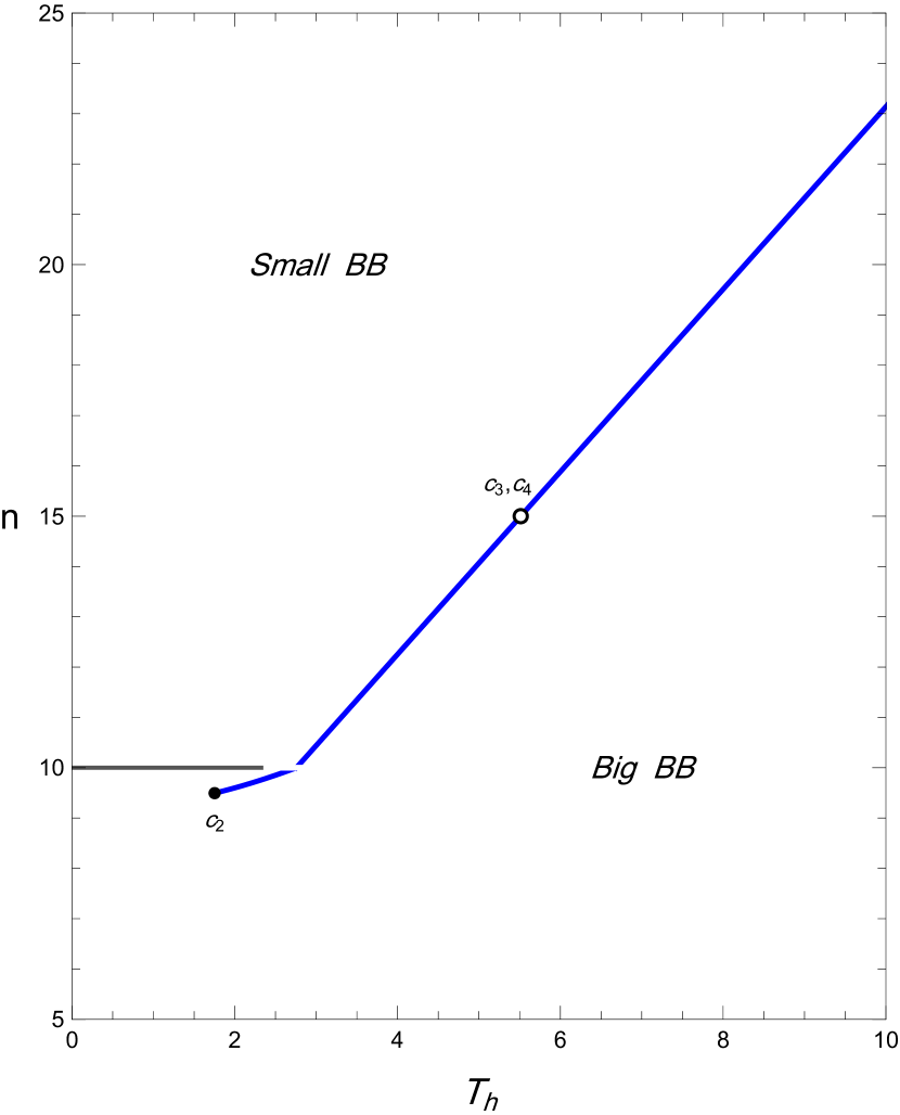
(b)

Figure 3.19: The $n-T$ phase diagram for case III.II where two of the critical points merge. Values used to draw this graph are ($l=1$, $\phi_{e}=15$, $\alpha=1$, $\widetilde{Q}_{m}=150$) The gray line at $n=n_{hp}$ shows the region where no black brane can exist.

Case III.III: $\absolutevalue{\widetilde{Q}_{m}}>\frac{l\phi_{e}^{2}\left(1+3\alpha^{2}\right)}{6}$

As the value of $\absolutevalue{\widetilde{Q}_{m}}$ increases to be greater than $\frac{l\phi_{e}^{2}\left(1+3\alpha^{2}\right)}{6}$ the two merged critical points vanish completely and the case becomes exactly the same as Case II.III.

4 Conclusion

We started with a review of the phase structure of the NUT-less dyonic black branes in the mixed ensemble, i.e. an ensemble with fixed electric potential and magnetic charge. Also, we have calculated the thermodynamic quantities of the solution and show that they obey the first law and Gibbs-Duhem relation. We showed that in the NUT-less case the phase structure is trivial since there are no phase transitions and the temperature is a monotonic function of the black hole horizon radius.

In the main work of the paper we have applied the thermodynamic treatment introduced in [33, 34] to the dyonic-NUT-AdS spacetimes with flat horizons to obtain various thermodynamic quantities. We showed that these quantities satisfy the first law as well as the Gibbs-Duhem relation. It was intriguing to notice that the first law is satisfied by a larger class of charges and potentials which depends on some additional arbitrary parameter $\alpha$ which in turn affects the phase structure. We analyzed the phase structure of these solutions through a mixed ensemble where we described the phase diagrams as NUT parameter-temperature graphs to show possible transitions between big and small black hole phases. We showed that due to the absence of Misner strings, one doesn’t need to fix $\alpha$, therefore, it takes any value [35]. Depending on the value of $\alpha$, one can classify the phase study into different distinct cases which could be further split into few sub-cases depending on the value of the other thermodynamic quantities. In most of these cases we have first-order phase transitions which end at one or more critical points. We found that these classes could have up to four critical points, again, depending on $\alpha$. It is important to notice that these phase structures are qualitatively different from the van der Waals structure of the liquid-gas phase transition.

One possible extension to this work is to study the Kerr-Newman-NUT in Minkowski as well as Anti-de Sitter spaces, which could enrich our understanding of the thermodynamics of the NUT-AdS spaces and their phase structure. Another extension of this work could be investigating the Plebanski-Demianski metric, a class of solutions that depends on seven parameters: mass, rotation, electric and magnetic charges, nut, acceleration, and cosmological constant. We hope that we can study one of these spacetimes in another work in the near future.

References

- Hawking and Page [1983] S. W. Hawking and D. N. Page, Commun. Math. Phys. 87, 577 (1983).
- Witten [1998] E. Witten, Adv. Theor. Math. Phys. 2, 253 (1998), hep-th/9802150.
- Chamblin et al. [1999a] A. Chamblin, R. Emparan, C. V. Johnson, and R. C. Myers, Phys. Rev. D 60, 064018 (1999a), hep-th/9902170.
- Chamblin et al. [1999b] A. Chamblin, R. Emparan, C. V. Johnson, and R. C. Myers, Phys. Rev. D 60, 104026 (1999b), hep-th/9904197.
- Vanzo [1997] L. Vanzo, Phys. Rev. D 56, 6475 (1997), gr-qc/9705004.
- Birmingham [1999] D. Birmingham, Class. Quant. Grav. 16, 1197 (1999), hep-th/9808032.
- Brill et al. [1997] D. R. Brill, J. Louko, and P. Peldan, Phys. Rev. D 56, 3600 (1997), gr-qc/9705012.
- Dutta et al. [2013] S. Dutta, A. Jain, and R. Soni, JHEP 12, 060 (2013), 1310.1748.
- Hartnoll et al. [2008a] S. A. Hartnoll, C. P. Herzog, and G. T. Horowitz, Phys. Rev. Lett. 101, 031601 (2008a), 0803.3295.
- Hartnoll et al. [2008b] S. A. Hartnoll, C. P. Herzog, and G. T. Horowitz, JHEP 12, 015 (2008b), 0810.1563.
- Horowitz and Roberts [2009] G. T. Horowitz and M. M. Roberts, JHEP 11, 015 (2009), 0908.3677.
- Hennigar [2017] R. A. Hennigar, JHEP 09, 082 (2017), 1705.07094.
- Chamblin et al. [1999c] A. Chamblin, R. Emparan, C. V. Johnson, and R. C. Myers, Phys. Rev. D 59, 064010 (1999c), hep-th/9808177.
- Emparan et al. [1999] R. Emparan, C. V. Johnson, and R. C. Myers, Phys. Rev. D 60, 104001 (1999), hep-th/9903238.
- Page and Pope [1987] D. N. Page and C. N. Pope, Class. Quant. Grav. 4, 213 (1987).
- Awad and Chamblin [2002] A. Awad and A. Chamblin, Class. Quant. Grav. 19, 2051 (2002), hep-th/0012240.
- Misner [1963] C. W. Misner, J. Math. Phys. 4, 924 (1963).
- Mann [1999] R. B. Mann, Phys. Rev. D 60, 104047 (1999), hep-th/9903229.
- Clarkson et al. [2003] R. Clarkson, L. Fatibene, and R. B. Mann, Nucl. Phys. B 652, 348 (2003), hep-th/0210280.
- Astefanesei et al. [2005] D. Astefanesei, R. B. Mann, and E. Radu, JHEP 01, 049 (2005), hep-th/0407110.
- Bordo et al. [2019a] A. B. Bordo, F. Gray, R. A. Hennigar, and D. Kubizňák, Class. Quant. Grav. 36, 194001 (2019a), 1905.03785.
- Bordo et al. [2019b] A. B. Bordo, F. Gray, and D. Kubizňák, JHEP 07, 119 (2019b), 1904.00030.
- Chen and Jiang [2019] Z. Chen and J. Jiang, Phys. Rev. D 100, 104016 (2019), 1910.10107.
- Hennigar et al. [2019] R. A. Hennigar, D. Kubizňák, and R. B. Mann, Phys. Rev. D 100, 064055 (2019), 1903.08668.
- Ballon Bordo et al. [2019] A. Ballon Bordo, F. Gray, R. A. Hennigar, and D. Kubizňák, Phys. Lett. B 798, 134972 (2019), 1905.06350.
- Wu and Wu [2019] S.-Q. Wu and D. Wu, Phys. Rev. D 100, 101501 (2019), 1909.07776.
- Ballon Bordo et al. [2020] A. Ballon Bordo, F. Gray, and D. Kubizňák, JHEP 05, 084 (2020), 2003.02268.
- Durka [2022] R. Durka, Int. J. Mod. Phys. D 31, 2250021 (2022), 1908.04238.
- Frodden and Hidalgo [2022] E. Frodden and D. Hidalgo, Phys. Lett. B 832, 137264 (2022), 2109.07715.
- Awad and Eissa [2020] A. Awad and S. Eissa, Phys. Rev. D 101, 124011 (2020), 2007.10489.
- Mann et al. [2021] R. B. Mann, L. A. Pando Zayas, and M. Park, JHEP 03, 039 (2021), 2012.13506.
- Abbasvandi et al. [2021] N. Abbasvandi, M. Tavakoli, and R. B. Mann, JHEP 08, 152 (2021), 2107.00182.
- Awad and Eissa [2022] A. Awad and S. Eissa, Phys. Rev. D 105, 124034 (2022), 2206.09124.
- Awad and Elkhateeb [2023] A. Awad and E. Elkhateeb, Phys. Rev. D 108, 064022 (2023), 2304.06705.
- Tharwat et al. [2024] M. Tharwat, A. AlBarqawy, A. Awad, and E. Elkhateeb, Phys. Rev. D 109, 084026 (2024), 2312.15811.
- Bonnor [1969] W. B. Bonnor, Math. Proc. Cambridge Phil. Soc. 66, 145 (1969).
- Hawking and Ross [1995] S. W. Hawking and S. F. Ross, Phys. Rev. D 52, 5865 (1995), hep-th/9504019.
- Gibbons and Hawking [1977] G. W. Gibbons and S. W. Hawking, Phys. Rev. D 15, 2752 (1977).
- Hartle and Hawking [1976] J. B. Hartle and S. W. Hawking, Phys. Rev. D 13, 2188 (1976).
- Gibbons and Perry [1978] G. W. Gibbons and M. J. Perry, Proc. Roy. Soc. Lond. A 358, 467 (1978).
- Kastor et al. [2009] D. Kastor, S. Ray, and J. Traschen, Class. Quant. Grav. 26, 195011 (2009), 0904.2765.
- Surya et al. [2001] S. Surya, K. Schleich, and D. M. Witt, Phys. Rev. Lett. 86, 5231 (2001), hep-th/0101134.