On the Interpolation Effect of Score Smoothing

Abstract

Score-based diffusion models have achieved remarkable progress in various domains with the ability to generate new data samples that do not exist in the training set. In this work, we examine the hypothesis that their generalization ability arises from an interpolation effect caused by a smoothing of the empirical score function. Focusing on settings where the training set lies uniformly in a one-dimensional linear subspace, we study the interplay between score smoothing and the denoising dynamics with mathematically solvable models. In particular, we demonstrate how a smoothed score function can lead to the generation of samples that interpolate among the training data within their subspace while avoiding full memorization. We also present evidence that learning score functions with regularized neural networks can have a similar effect on the denoising dynamics as score smoothing.

1 Introduction

In recent years, score-based diffusion models (DMs) have become an important pillar of generative modeling across a variety of domains from content generation to scientific computing (Sohl-Dickstein et al.,, 2015; Song and Ermon,, 2019; Ho et al.,, 2020; Ramesh et al.,, 2022; Abramson et al.,, 2024; Brooks et al.,, 2024). After being trained on datasets of actual images or molecular configurations, for instance, such models can transform noise samples into high-quality images or chemically-plausible molecules that do not belong to the training set, indicating an exciting capability of such models to generalize beyond what they have seen and, in a sense, be “creative”.

The mechanism behind the creativity of score-based DMs has been a topic of much theoretical interests. At the core of these models is the training of neural networks (NNs) to fit a series of target functions, often called the empirical score functions (ESFs), which are used to drive the denoising process at inference time. The precise form of these functions are determined by the training set and can be computed exactly in principle (though inefficient in practice), but when equipped with the exact precise ESF instead of the approximate version learned by NNs, the diffusion model will end up generate data points that already exist in the training set (Yi et al.,, 2023; Li et al., 2024a, ), a phenomenon commonly called memorization. This suggests that, for the models to generalize fresh samples beyond the training set, it is crucial to have certain regularizations on the score function (e.g., through NN training) that prevent the ESF from being learned exactly. From the viewpoint of density estimation, a number of important works have proved sample complexity guarantees for the estimation of score functions via regularized models (discussed in Section 7). However, as these results are often specialized for specific underlying distributions and model families, the probe into a more general and intuitive mechanism behind generalization in DMs is still largely open.

A particularly interesting hypothesis by Scarvelis et al., (2023) is that smoothing the ESF allows the model to generate samples that interpolate among training data points, which helps to achieve generalization. With this insight, they proposed alternative DMs based on computing the smoothed ESF explicitly, but a thorough understanding of the effect of score smoothing on the denoising dynamics was still lacking. On a different yet closely related front, to understand the hallucination phenomenon in DM, Aithal et al., (2024) observed that the models generate samples which interpolate between modes of the training distribution when the NN learns a smoother version of the ESF, but the theoretical mechanism behind this phenomenon also remains unclear.

In this work, we study the effect of score smoothing on the denoising dynamics mathematically and show how it can lead to data interpolation and subspace recovery in simple cases. Specifically,

1. When the training data are spaced uniformly in $1$-D, we show that the denoising dynamics under the smoothed score recovers a non-singular density that interpolates the training set;

2. If the $1$-D subspace is embedded in higher dimensions, we show that the denoising dynamics under the smoothed score converges to a non-singular interpolating density on the relevant subspace;

3. We give theoretical and empirical evidence that the our analysis based on score smoothing is relevant for understanding how NN-based DMs avoid memorization.

Together, we believe these results shed light on how score smoothing can be an important causal link for understanding how NN-based DMs avoid memorization and motivate the exploration of alternative designs of DMs that generalize.

The rest of the paper is organized as follows. After briefly reviewing the background in Section 2, we examine the smoothing of ESF in the one-dimensional ($1$-D) case and discuss its connections with NN regularization in Section 3. The trajectory of the denoising dynamics under the smoothed score is derived in Section 4. In Section 5, we generalize the analysis to the higher-dimensional case when the training data belongs to a hidden line segment. In Section 6, we provide experimental evidence that NN-learned SF also exhibits an interpolation effect that is similar to that of score smoothing.

Notations

For $x,\delta>0$, we write $p_{\mathcal{N}}(x;\sigma)=(\sqrt{2\pi}\sigma)^{-1}\exp(-x^{2}/(2\sigma^{2}))$ denote the $1$-D Gaussian density with mean zero and variance $\sigma^{2}$; $\bm{\delta}_{x}$ for the Dirac delta distribution centered at $x\in{\mathbb{R}}$; and $\text{sgn}(x)$ for the sign of $x$. We write $[n]\coloneqq\{1,..,n\}$ for $n\in{\mathbb{N}}_{+}$. For a vector ${\bm{x}}=[x_{1},...,x_{d}]\in{\mathbb{R}}^{d}$, we write $[{\bm{x}}]_{i}=x_{i}$ for $i\in[d]$. The use of big-O notations is explained in Appendix A.

2 Background

While score-based DMs have many variants, we will focus on a basic one (called the “Variance Exploding” version in Song et al., 2021b ) for simplicity, where the forward (or noising) process is defined by the following stochastic differential equation (SDE) in ${\mathbb{R}}^{d}$ for $t\geq 0$:

$$d{\mathbf{x}}_{t}=d{\mathbf{w}}_{t}~,\quad{\mathbf{x}}_{0}\sim p_{0}~,$$ (1)

where ${\mathbf{w}}$ is the Wiener process (a.k.a. Brownian motion) in ${\mathbb{R}}^{d}$. The marginal distribution of ${\mathbf{x}}_{t}$, denoted by $p_{t}$, is thus fully characterized by the initial distribution $p_{0}$ together with the conditional distribution, $p_{t|0}({\bm{x}}|{\bm{x}}^{\prime})=\prod_{i=1}^{d}p_{\mathcal{N}}([{\bm{x}}]_{i}-[{\bm{x}}^{\prime}]_{i};\sqrt{t})$. In other words, $p_{t}$ is obtained by convolving $p_{0}$ with an isotropic Gaussian distribution with variance $\sigma(t)^{2}=t$ in every direction.

A key observation is that this process is equivalent (in marginal distribution) to a deterministic dynamics often called the probability flow ordinary differential equation (ODE) (Song et al., 2021b, ):

$$d{\mathbf{x}}_{t}= ~-\tfrac{1}{2}{\bm{s}}_{t}({\mathbf{x}}_{t})dt~,$$ (2)

where ${\bm{s}}_{t}({\mathbf{x}})=\nabla\log p_{t}({\mathbf{x}})$ is the score function (SF) associated with the distribution $p_{t}$ (Hyvärinen and Dayan,, 2005). In generative modeling, $p_{0}$ is often a distribution of interest that is hard to sample directly (e.g. the distribution of cat images in pixel space), while when $T$ is large, $p_{T}$ is always close to a Gaussian distribution (with variance increasing in $T$), from which samples are easy to obtain. Thus, to obtain samples from $p_{0}$, a insightful idea is to first sample from $p_{T}$ and then follow the reverse (or denoising) process by simulating (2) backward-in-time (or its stochastic variants that are equivalent in marginal distribution, which we will not focus on.

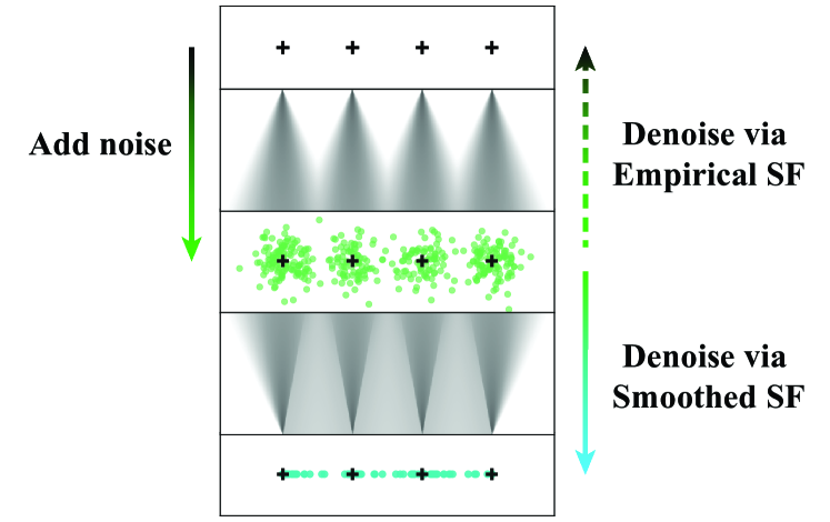
Figure 1: From the noised empirical distribution (i.e., $p^{(n)}_{t_{0}}$; middle), running the denoising dynamics (2) using the ESF (${\bm{s}}_{t}=\nabla\log p^{(n)}_{t}$) leads back to the empirical distribution of the training set (i.e., $p^{(n)}_{0}$; top), whereas using a smoothed SF (e.g. the LA-PL SF, ${\bm{s}}_{t}=\hat{{\bm{s}}}^{(n)}_{t,\delta_{t}}$; or NN-learned) produces a distribution that interpolates among the training set on the relevant subspace (e.g., $\hat{p}^{(n,t_{0})}_{0}$ in the case of LA-PL SF; bottom).

A main challenge in this procedure lies in the estimation of the family of SFs, $\nabla\log p_{t}$ for $t\in[0,T]$. In reality, we have no prior knowledge of each $p_{t}$ (or even $p_{0}$) but just a training set $S=\{{\bm{y}}_{k}\}_{k\in[n]}$ usually assumed to be sampled from $p_{0}$. Thus, we only have access to an empirical version of the noising process, where the same SDE (1) is initialized at $t=0$ with not $p_{0}$ but the uniform distribution over $S$ (i.e., ${\mathbf{x}}_{0}\sim p^{(n)}_{0}\coloneqq\frac{1}{n}\sum_{k=1}^{n}\delta_{{\bm{y}}_{k}}$), and hence the marginal distribution of ${\mathbf{x}}_{t}$ is $p^{(n)}_{t}({\bm{x}})\coloneqq\frac{1}{n}\sum_{k=1}^{n}p_{t|0}({\bm{x}}|{\bm{y}}_{k})$, called the noised empirical distribution at time $t$. To obtain a proxy for $\nabla\log p_{t}$, one often uses an NN to represent a (time-dependent) score estimator, $s_{\bm{\theta}}({\bm{x}},t)$, and train its parameters to minimize variants of the following time-averaged score matching loss (Song et al., 2021b, ):

$$\min_{\bm{\theta}}\frac{1}{T}\int_{0}^{T}L^{(n)}_{t}[s_{\bm{\theta}}(~\cdot~,t)]dt~,$$ (3)

where

$$L^{(n)}_{t}[f]\coloneqq t\cdot{\mathbb{E}}_{{\mathbf{x}}\sim p^{(n)}_{t}}\Big{[}\big{\|}f({\mathbf{x}})-\nabla\log p^{(n)}_{t}({\mathbf{x}})\big{\|}^{2}\Big{]}~$$ (4)

measures the $L^{2}$ distance between the score estimator and the empirical score function (ESF) at time $t$ — $\nabla\log p^{(n)}_{t}$ — with respect to $p^{(n)}_{t}$. The scaling factor of $t\propto 1/{\mathbb{E}}[\nabla\log p_{t|0}({\mathbf{x}}_{t}|{\mathbf{x}}_{0})]$ serves to balance the contribution to the loss at different $t$ (Song et al., 2021b, ).

In practice, the minimization problem (3) is often solved via Monte-Carlo sampling combined with ideas from Hyvärinen and Dayan, (2005); Vincent, (2011). However, we know the minimum is attained uniquely by the ESF itself, which can be computed in closed form based on $S$ (details in Section 3). So what if we use the ESF directly in the denoising dynamics (2) instead of an NN approximation? In that case, we arrive at an empirical version of the probability flow ODE:

$$d{\mathbf{x}}_{t}=-\tfrac{1}{2}\nabla\log p^{(n)}_{t}({\mathbf{x}}_{t})~,$$ (5)

which exactly reverses the empirical forward process that adds noise to the training set, and hence the outcome at $t=0$ is inevitably $p^{(n)}_{0}$. In other words, the model memorizes the training data instead of generating fresh samples. This suggests that the creativity of the diffusion model hinges on a sub-optimal solution to the minimization problem (3) and an imperfect approximation to the ESF. Indeed, the memorization phenomenon has been observed in practice when the models have large capacities relative to the training set size (Gu et al.,, 2023; Kadkhodaie et al.,, 2024), which likely results in too good an approximation to the ESF. This leads to the hypothesis that regularizing the score estimator gives rise to the model’s ability to generalize out of the training set, though a theoretical understanding of the mechanism is still under development.

In this work, we will focus on simple setups with fixed training sets to show mathematically how smoothing the ESF can enable the generation of new samples that interpolate among the training data.

3 Score Function and its Smoothing

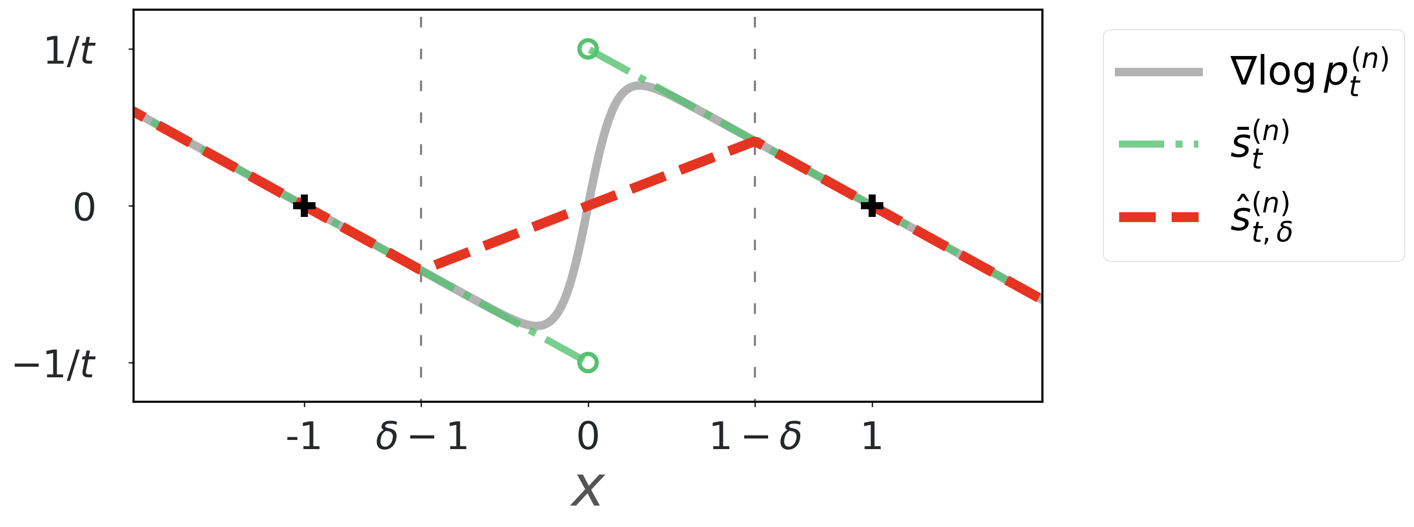
Figure 2: Comparing the ESF, $\nabla\log p^{(n)}_{t}$; its PL approximation (8), $\bar{s}^{(n)}_{t}$; and the LA-PL SF (31), $\hat{s}^{(n)}_{t,\delta}$ in the case of $d=1$ and $n=2$ discussed in Section 3.

Let us focus on a simplest setup where $d=1$ and $S=\{y_{1}=-1,y_{2}=1\}$ consists of only two points. In Appendix C, we give a straightforward generalization of the analyses in Sections 3 - 5 to the scenario where $S$ consists of $n$ points spaced uniformly on an interval $[-D,D]$.

In the $n=2$ case, at time $t$, the noised empirical distribution is $p^{(n)}_{t}(x)=\frac{1}{2}(p_{\mathcal{N}}(x+1;\sqrt{t})+p_{\mathcal{N}}(x-1;\sqrt{t}))$, and the (scalar-valued) ESF takes the form of

$$\tfrac{d}{dx}\log p^{(n)}_{t}(x)=(\hat{x}^{(n)}_{t}(x)-x)/t~,$$ (6)

where

$$\hat{x}^{(n)}_{t}(x)\coloneqq{\mathbb{E}}_{0|t}[{\mathbf{x}}_{0}|{\mathbf{x}}_{t}=x]=\tfrac{p_{\mathcal{N}}(x-1;\sqrt{t})-p_{\mathcal{N}}(x+1;\sqrt{t})}{p_{\mathcal{N}}(x-1;\sqrt{t})+p_{\mathcal{N}}(x+1;\sqrt{t})}$$ (7)

lies between $\pm 1$ and has the same sign as $x$. When $t$ decreases, the Gaussians sharpen and $\hat{x}^{(n)}_{t}(x)$ approaches $\text{sgn}(x)$, allowing us to approximate the ESF by a piece-wise linear (PL) function,

$$\bar{s}^{(n)}_{t}(x)=(\text{sgn}(x)-x)/t~.$$ (8)

It is then intuitive that the backward dynamics is attracted to either of $\pm 1$ (whichever is closer) thus explaining the collapse onto the training set when we denoise with the exact ESF. Hence, to avoid memorization, one needs to go beyond the exact ESF for driving the denoising dynamics.

In this work, we will mainly focus on the following family of SF and study its effect on the denoising dynamics (2) when $t$ is small:

$$\hat{s}^{(n)}_{t,\delta}(x)\coloneqq\begin{cases}-(x+1)/t~,&\quad\text{ if }x\leq\delta-1~,\\ -(x-1)/t~,&\quad\text{ if }x\geq 1-\delta~,\\ \delta/(1-\delta)\cdot x/t~,&\quad\text{ if }x\in(\delta-1,1-\delta)~.\end{cases}$$ (9)

where $\delta\in(0,1]$ can be chosen to depend on $t$. As illustrated in Figure 2, $\hat{s}^{(n)}_{t,\delta}$ is PL and matches $\bar{s}^{(n)}_{t}$ except on the interval $[\delta-1,1-\delta]$. When $\delta=1$, $\hat{s}^{(n)}_{t,1}\equiv\bar{s}^{(n)}_{t}$. When $\delta\in(0,1)$, as will be made clear in Section 3.1, we refer to $\hat{s}^{(n)}_{t,\delta}$ as a locally-averaged piece-wise-linearized (LA-PL) SF.

In the rest of this section, based on connections with function smoothing and NN learning, we discuss two motivations for studying the LA-PL SF (especially under a specific choice of $\delta$ as a function of $t$) as a smoothed estimator for the ESF.

3.1 Connection to Function Smoothing via Local Averaging

Given a function $f$ on ${\mathbb{R}}$ and $w>0$, we define a locally-averaged (LA) version of $f$ with window size $w$ to be the following function:

$$(w*f)(x)\coloneqq\frac{1}{2w}\int_{x-w}^{x+w}f(x^{\prime})dx^{\prime}~.$$ (10)

It is then not hard to see that, for $w\in(0,1]$,

$$(w*\bar{s}^{(n)}_{t})(x)=\hat{s}^{(n)}_{t,1-w}(x)~,\quad\forall x\in{\mathbb{R}}~.$$ (11)

This explains the naming of $\hat{s}^{(n)}_{t,\delta}$. In particular, a smaller $\delta$ means a higher level of local smoothing.

As $\bar{s}^{(n)}_{t}$ approximates the ESF when $t$ is small, we expect from (11) that $\hat{s}^{(n)}_{t,\delta}$ is also close to $(1-\delta)*\tfrac{d}{dx}\log p^{(n)}_{t}$. This can be made rigorous in the setting where $\delta$ is fixed while $t\to 0$, in which case the $L^{2}$ distance with respect to $p^{(n)}_{t}$ between the two functions decays exponentially fast in $1/t$ (proved in Appendix D):

Lemma 1

For any fixed $\delta\in(0,1]$, $\exists t_{1},C>0$ such that $\forall t\in(0,t_{1})$, it holds that

$$t\cdot{\mathbb{E}}_{x\sim p^{(n)}_{t}}\Big{[}\big{\|}\hat{s}^{(n)}_{t,\delta}(x)-((1-\delta)*\tfrac{d}{dx}\log p^{(n)}_{t})(x)\big{\|}^{2}\Big{]}\leq C\exp(-\delta^{2}/(9t))~.$$ (12)

This result motivates us to focus on $\hat{s}^{(n)}_{t,\delta}$ as a simpler proxy for understanding the smoothed ESF.

Coupling $\delta$ with $t$

Our subsequent analysis on the dynamics will focus on the LA-PL SF under a time-dependent $\delta$ that is chosen proportionally to $\sqrt{t}$, i.e., for some $\kappa>0$,

$$\delta_{t}=\kappa\sqrt{t}~,$$ (13)

corresponding to choosing a larger window size for LA as $t$ decreases. To motivate this choice, we observe that as $t\to 0$, the empirical distribution $p^{(n)}_{t}$ becomes increasingly concentrated near $\pm 1$, and hence for any fixed $\delta$, the difference between two functions on $[\delta-1,1-\delta]$ contributes less and less to their $L^{2}$ distance with respect to $p^{(n)}_{t}$. In fact, the following result (proved in Appendix E) shows that as $t\to 0$, the score matching loss still remains at a constant order even if we let $\delta_{t}$ decrease according to (13):

Proposition 2

Let $\delta_{t}=\kappa\sqrt{t}$ for some $\kappa>0$. Then $\exists t_{1},C>0$ such that $\forall t\in(0,t_{1})$,

$$\tfrac{1}{2}F(\kappa)-C\sqrt{t}\leq L^{(n)}_{t}[\hat{s}^{(n)}_{t,\delta_{t}}]\leq\tfrac{1}{2}F(\kappa)+C\sqrt{t}~,$$ (14)

where $t_{1}$ and $C$ depend only on $\kappa$ and the function $F$ decreases strictly from $1$ to $0$ on $[0,\infty)$.

Thus, if we choose $\hat{s}^{(n)}_{t,\delta_{t}}$ as the score estimator and set (13), then the time-averaged score matching loss (3) has roughly balanced contributions from different $t$ when $t$ is small.

3.2 Connection to Smoothness Measure Induced by NN Regularization

When fitting a function in one dimension, it is shown in Savarese et al., (2019) that controlling the weight norm of a two-layer ReLU NN (with unregularized bias and linear terms) is essentially equivalent to penalizing a certain non-smoothness measure of the estimated function defined as:

$$R[f]\coloneqq\int_{-\infty}^{\infty}|f^{\prime\prime}(x)|dx~,$$ (15)

where $f^{\prime\prime}$ is the weak second derivative of the function $f$. Inspired by this result, for $\epsilon,t>0$, we consider the following family of variational problems in function space:

$$\begin{split}r_{t,\epsilon}^{*}\quad\coloneqq\quad\inf_{f}\qquad&R[f]\\ \text{s.t.}\qquad&L^{(n)}_{t}[f]\leq\epsilon~,\end{split}$$ (16)

with the infimum taken over all functions $f$ on ${\mathbb{R}}$ that are twice differentiable except on a finite set (a broad class of functions that include, for example, any function representable by a finite-width NN). Thus, we are seeking to minimize the non-smoothness measure among functions that are $\epsilon$-close to the ESF according to the $L^{2}$ distance with respect to $p^{(n)}_{t}$. When $\epsilon=0$, only the ESF itself satisfies the constraint and hence it attains the minimum uniquely; whereas if $\epsilon$ is small but positive, this problem is concerned with on how the non-smoothness penalty biases the score estimator away from the ESF.

Due to non-differentiability of the functional $R$, the variational problem (16) is hard to solve directly. However, we can show that the series of functions $\hat{s}^{(n)}_{t,\delta_{t}}$ together with (13) achieves near optimality in the following sense:

Proposition 3

Given any fixed $\epsilon\in(0,0.015)$, if we choose $\delta_{t}=\kappa\sqrt{t}$ with any $\kappa\geq F^{-1}(\epsilon)$, then there exists $t_{1}>0$ (dependent on $\kappa$) such that the following holds for all $t\in(0,t_{1})$:

• $L^{(n)}_{t}[\hat{s}^{(n)}_{t,\delta_{t}}]<\epsilon$, and hence the function $\hat{s}^{(n)}_{t,\delta_{t}}$ belongs to the feasible set of (16);

• $R[\hat{s}^{(n)}_{t,\delta_{t}}]<(1+8\sqrt{\epsilon})r_{t,\epsilon}^{*}$.

The proof is given in Appendix F and based on the following observation: When $t$ is small, the empirical distribution $p^{(n)}_{t}$ is concentrated near $\{\pm 1\}$, and hence for any function belonging to the feasible set with a small enough $\epsilon$, its derivative near $\pm 1$ needs to be close to $\frac{d}{dx}\log p^{(n)}_{t}(\pm 1)\approx-1/t$. Combined with the fundamental theorem of calculus, this allows us to give a lower bound on $r^{*}_{t,\epsilon}$.

As $\epsilon$ controls the strength of the regularization relative to the score matching loss, this setting (fixed $\epsilon$ for different $t$) could be interpreted heuristically as having similar “amount” of regularization to the score estimator at different $t$, though the precise correspondence remains to be further elucidated in future work. Meanwhile, in Section 6, we show empirical evidence that a regularized NN can indeed learn a SF that is close to $\hat{s}^{(n)}_{t,\delta_{t}}$.

4 Effect on the Denoising Dynamics

With the motivations discussed above, we now study the effect on the denoising dynamics of substituting the ESF (6) with $\hat{s}^{(n)}_{t,\delta_{t}}$ where $\delta_{t}=\kappa\sqrt{t}$ for some $\kappa>0$, that is, replacing (5) by:

$$\tfrac{d}{dt}{\mathbf{x}}_{t}=-\tfrac{1}{2}\hat{s}^{(n)}_{t,\delta_{t}}({\mathbf{x}}_{t})~.$$ (17)

Thanks to the piece-wise linearity of (9), the backward-in-time dynamics of the ODE (17) can be solved analytically in terms of flow maps:

Proposition 4

For $0\leq s\leq t<1/\kappa^{2}$, the solution to (17) satisfies ${\mathbf{x}}_{s}=\phi_{s|t}({\mathbf{x}}_{t})$, where

$$\phi_{s|t}(x)=\begin{cases}(1-\delta_{s})/(1-\delta_{t})\cdot x~,&\quad\text{ if }x\in[\delta_{t}-1,1-\delta_{t}]\\ \sqrt{s}/\sqrt{t}\cdot x-(1-\sqrt{s}/\sqrt{t})~,&\quad\text{ if }x\leq\delta_{t}-1\\ \sqrt{s}/\sqrt{t}\cdot x+(1-\sqrt{s}/\sqrt{t})~,&\quad\text{ if }x\geq 1-\delta_{t}\\ \end{cases}$$ (18)

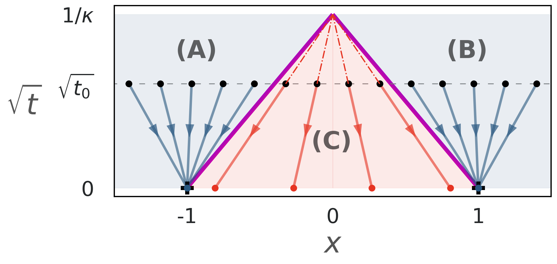
Figure 3: Phase diagram in the $x$-$\sqrt{t}$ plane for the flow solution (18) of the dynamics (17) in the $d=1$, $n=2$ case analyzed in Section 4.

The proposition is proved in Appendix H, and we illustrate the trajectories characterized by $\phi_{s|t}$ in Figure 3. The PL nature of $\hat{s}^{(n)}_{t,\delta_{t}}$ divides the $x-\sqrt{t}$ plane into three regions (A, B and C) with linear boundaries, each defined by $x\leq-1+\delta_{t}$, $x\geq 1-\delta_{t}$ and $\delta_{t}-1\leq x\leq 1-\delta_{t}$, respectively. Importantly, trajectories given by $\phi_{s|t}$ do not cross the region boundaries. If at $t_{0}>0$, ${\mathbf{x}}_{t_{0}}$ falls into region A (or B), then as $t$ decreases to $0$, it will follow a linear path in the $x-\sqrt{t}$ plane to $y_{1}=-1$ (or $y_{2}=1$). Meanwhile, if ${\mathbf{x}}_{t_{0}}$ falls into region C, then it will follow a linear path to the $x$-axis with a terminal value between $-1$ and $1$, which is given by

$$\phi_{0|t}(x)=\begin{cases}x/(1-\delta_{t})~,&\quad\text{ if }x\in[\delta_{t}-1,1-\delta_{t}]\\ \text{sgn}(x)~,&\quad\text{ otherwise}\\ \end{cases}$$ (19)

Now, we examine the evolution of the marginal distribution in light of the flow solution above. Suppose we run the denoising dynamics (17) backward-in-time from some $t_{0}\in(0,1/\kappa^{2})$ to $0$ and denote the marginal distribution of ${\mathbf{x}}_{t}$ by $\hat{p}^{(n,t_{0})}_{t}$ for $t\in[0,t_{0}]$. We assume that $\hat{p}^{(n,t_{0})}_{t_{0}}=p^{(n)}_{t_{0}}$ is the noised empirical distribution at time $t_{0}$. This can be viewed as starting from the noised empirical distribution at some large time $T$ (nearly Gaussian), first running the denoising process via the ESF until time $t_{0}$, and then switching to the LA-PL SF to drive the rest of the denoising process to time zero. In other words, score smoothing kicks in only when $t\in(0,t_{0})$. Another equivalent interpretation is that we add noise to the training data for time $t_{0}$ before denoising them with the LA-PL SF for the same amount (as illustrated in Figure 1).

For $0<s\leq t\leq t_{0}$, since the map $\phi_{s|t}$ is invertible and differentiable almost everywhere, we can apply the change-of-variable formula of push-forward distributions to obtain that

$$\hat{p}^{(n,t_{0})}_{s}(x)=\begin{cases}(1-\delta_{t})/(1-\delta_{s})\cdot\hat{p}^{(n,t_{0})}_{t}((1-\delta_{t})/(1-\delta_{s})\cdot x)~,&\text{if }x\in[\delta_{s}-1,1-\delta_{s}]\\ \delta_{t}/\delta_{s}\cdot\hat{p}^{(n,t_{0})}_{t}(\delta_{t}/\delta_{s}\cdot x+(\delta_{t}-\delta_{s})/\delta_{s})~,&\text{if }x\leq\delta_{s}-1\\ \delta_{t}/\delta_{s}\cdot\hat{p}^{(n,t_{0})}_{t}(\delta_{t}/\delta_{s}\cdot x-(\delta_{t}-\delta_{s})/\delta_{s})~,&\text{if }x\geq 1-\delta_{s}\end{cases}$$ (20)

The evolution of the density $\hat{p}^{(n,t_{0})}_{s}$ as $s$ decreases from $t_{0}$ to $0$ is visualized in the lower grey-colored heat map in Figure 1. When $s=0$, $\phi_{0|t}$ is invertible only when restricted to $[\delta_{t}-1,1-\delta_{t}]$, Thus, the terminal distribution can be decomposed as

$$\hat{p}^{(n,t_{0})}_{0}=a_{+}\bm{\delta}_{1}+a_{-}\bm{\delta}_{-1}+(1-a_{+}-a_{-})\tilde{p}^{(n,t_{0})}_{0}~,$$ (21)

where $\tilde{p}^{(n,t_{0})}_{0}$ is a probability distribution and for all $t\in(0,t_{0}]$, it holds that $a_{+}={\mathbb{E}}_{{\mathbf{x}}\sim\hat{p}^{(n,t_{0})}_{t}}[\mathds{1}_{{\mathbf{x}}\geq 1-\delta_{t}}]$, $a_{-}={\mathbb{E}}_{{\mathbf{x}}\sim\hat{p}^{(n,t_{0})}_{t}}[\mathds{1}_{{\mathbf{x}}\leq\delta_{t}-1}]$, and

$$\tilde{p}^{(n,t_{0})}_{0}(x)=\begin{cases}(1-\delta_{t})/(1-a_{+}-a_{-})\cdot\hat{p}^{(n,t_{0})}_{t}((1-\delta_{t})x)~,&\quad\text{ if }x\in[-1,1]\\ 0~,&\quad\text{ otherwise}\end{cases}$$ (22)

In particular, since $\hat{p}^{(n,t_{0})}_{t_{0}}$ has a positive density on $[\delta_{t_{0}}-1,1-\delta_{t_{0}}]$, $\tilde{p}^{(n,t_{0})}_{0}$ has a positive density on $[-1,1]$ as well, corresponding to a smooth interpolation between the two training data points.

Moreover, (22) allows us to prove KL-divergence bounds for $\hat{p}^{(n,t_{0})}_{0}$ based on those of $\hat{p}^{(n,t_{0})}_{t}$. For example, letting $u_{a}$ denote the uniform density on $[-a,a]$, we have:

Proposition 5

Let $\kappa>0$ and $0<t_{0}<1/\kappa^{2}$. If ${\mathbf{x}}_{t}$ solves (17) backward-in-time with ${\mathbf{x}}_{t_{0}}\sim p^{(n)}_{t_{0}}$, then there is $\text{KL}(u_{1}||\hat{p}^{(n,t_{0})}_{0})\leq\tfrac{1}{3t_{0}(1-\kappa\sqrt{t_{0}})}+\log\big{(}\tfrac{\sqrt{t_{0}}}{1-\kappa\sqrt{t_{0}}}\big{)}+\log(2\sqrt{2\pi})<\infty$.

This result is proved in Appendix I. We note that the choice of the uniform density as the target to compare $\hat{p}^{(n,t_{0})}_{0}$ with is an arbitrary one, since the training set is fixed rather than sampled from the uniform distribution. But our main point is to highlight the component of $\hat{p}^{(n,t_{0})}_{0}$ that smoothly interpolates among the training set. In contrast, running the entire denoising dynamics with the exact ESF results in $p^{(n)}_{0}$, which is fully singular and has an infinite KL-divergence with any smooth density on $[-1,1]$.

5 Higher Dimensions: Line Segment as Hidden Subspace

Let us consider a case where $S=\{{\bm{y}}_{1}=[-1,0,...,0],{\bm{y}}_{2}=[1,0,...,0]\}\subseteq{\mathbb{R}}^{d}$ consists of two points on the $[{\bm{x}}]_{1}$-axis (and as we show in Appendix C, the analysis can also be generalized to the case where $S$ contains $n$ points spaced uniformly on the $[{\bm{x}}]_{1}$-axis). In this case, the noised empirical density is $p^{(n)}_{t}({\bm{x}})=\frac{1}{2}\big{(}p_{\mathcal{N}}([{\bm{x}}]_{1}+1;\sqrt{t})+p_{\mathcal{N}}([{\bm{x}}]_{1}-1;\sqrt{t})\big{)}\prod_{i=2}^{d}p_{\mathcal{N}}([{\bm{x}}]_{i};\sqrt{t})$, and the (vector-valued) ESF is given by $\nabla\log p^{(n)}_{t}({\bm{x}})=[\partial_{1}\log p^{(n)}_{t}({\bm{x}}),...,\partial_{d}\log p^{(n)}_{t}({\bm{x}})]$, where

$$\begin{split}\partial_{1}\log p^{(n)}_{t}({\bm{x}})=&~\big{(}\hat{x}^{(n)}_{t}([{\bm{x}}]_{1})-[{\bm{x}}]_{1}\big{)}/t~,\\ \forall i\in\{2,...,n\}~,\quad\partial_{i}\log p^{(n)}_{t}({\bm{x}})=&~-[{\bm{x}}]_{i}/t~,\hskip 80.0pt\end{split}$$ (23)

where $\hat{x}^{(n)}_{t}$ is defined in the same way as in (7). Relative to the subspace on which the training set belongs — the $[{\bm{x}}]_{1}$-axis — we may refer to the first dimension as the tangent direction and the other dimensions as the normal directions.

To generalize the notion of score smoothing beyond dimension one, we first consider a simple extension of the definition (10) that takes averages over centered cubes in higher dimensions. Namely, given $w>0$ and a (vector-valued) function ${\bm{f}}$ on ${\mathbb{R}}^{d}$, we define

$$(w*{\bm{f}})({\bm{x}})=\frac{1}{(2w)^{d}}\int_{[{\bm{x}}]_{1}-w}^{[{\bm{x}}]_{1}+w}...\int_{[{\bm{x}}]_{d}-w}^{[{\bm{x}}]_{d}+w}{\bm{f}}({\bm{x}}^{\prime})d[{\bm{x}}^{\prime}]_{1}...d[{\bm{x}}^{\prime}]_{d}~.$$ (24)

To understand how the ESF behaves under (24), we first observe that for each $i\in[d]$, $\partial_{i}\log p^{(n)}_{t}({\bm{x}})$ depends only on the corresponding $x_{i}$, and hence the repeated integral in (24) reduces to only the one in the $i$th dimension. For $i>1$, $\partial_{i}\log p^{(n)}_{t}({\bm{x}})$ is a linear function of $[{\bm{x}}]_{i}$, which is invariant when averaged over a centered interval. For $i=1$, $w*\partial_{1}\log p^{(n)}_{t}({\bm{x}})$ has the same form as in the $d=1$ case after a projection onto the first dimension, which can therefore be approximated by $\hat{s}^{(n)}_{t,1-w}([{\bm{x}}]_{1})$ on the same theoretical ground as Lemma 1. In summary, for $w\in(0,1)$, we have

$$\begin{split}w*\nabla\log p^{(n)}_{t}({\bm{x}})=&~[w*\partial_{1}\log p^{(n)}_{t}({\bm{x}}),-[{\bm{x}}]_{2}/t,...,-[{\bm{x}}]_{d}/t]^{\intercal}\\ \approx&~[\hat{s}^{(n)}_{t,1-w}([{\bm{x}}]_{1}),-[{\bm{x}}]_{2}/t,...,-[{\bm{x}}]_{d}/t]^{\intercal}=\hat{{\bm{s}}}^{(n)}_{t,1-w}({\bm{x}})~,\end{split}$$ (25)

where for $\delta\in(0,1]$, we define a generalization of the LA-PL SF in this setting by

$$\hat{{\bm{s}}}^{(n)}_{t,\delta}({\bm{x}})\coloneqq[\hat{s}^{(n)}_{t,\delta}([{\bm{x}}]_{1}),-[{\bm{x}}]_{2}/t,...,-[{\bm{x}}]_{d}/t]^{\intercal}~,$$ (26)

with $\hat{s}^{(n)}_{t,\delta}:{\mathbb{R}}\to{\mathbb{R}}$ defined in the same way as in (9).

Similar to in Section 4, we consider a scenario where the smoothing level depends on time through $w_{t}=1-\delta_{t}$ with (13), in which case the dynamics is given by $\frac{d}{dt}{\mathbf{x}}_{t}=-\frac{1}{2}\hat{{\bm{s}}}^{(n)}_{t,\delta_{t}}({\mathbf{x}}_{t})$ and is nicely decoupled in different dimensions:

$$\tfrac{d}{dt}[{\mathbf{x}}_{t}]_{1}= ~-\tfrac{1}{2}\hat{s}^{(n)}_{t,\delta_{t}}([{\mathbf{x}}_{t}]_{1})~,$$ (27)

$$\forall i\in\{2,...,d\}~,\quad\tfrac{d}{dt}[{\mathbf{x}}_{t}]_{i}= ~\tfrac{1}{2}[{\mathbf{x}}_{t}]_{i}/t~.\hskip 80.0pt$$ (28)

Based on our findings in the $d=1$ case, we see that this dynamics can be solved as follows:

Proposition 6

For $0\leq s\leq t<1/\kappa^{2}$, the solution to (27, 28) is given by ${\mathbf{x}}_{s}=\Phi_{s|t}({\mathbf{x}}_{t})\coloneqq[\phi_{s|t}({\textnormal{x}}_{t,1}),0,...,0]$ with $\phi_{s|t}$ defined as in (18) and (19). Hence, if run backward-in-time with the marginal distribution of ${\mathbf{x}}_{t_{0}}$ being $\hat{p}^{(n,t_{0})}_{t_{0}}\times p_{\mathcal{N}}(~\cdot~;\sqrt{t_{0}})\times...\times p_{\mathcal{N}}(~\cdot~;\sqrt{t_{0}})$, the marginal distribution of ${\mathbf{x}}_{t}$ is given by $\hat{p}^{(n,t_{0})}_{t}\times p_{\mathcal{N}}(~\cdot~;\sqrt{t})\times...\times p_{\mathcal{N}}(~\cdot~;\sqrt{t})$, where $\hat{p}^{(n,t_{0})}_{t}$ satisfies (20) or (21).

Notably, we see distinct dynamical behaviors in the tangent versus normal directions. As $t\to 0$, the trajectory converges to zero at a rate of $\sqrt{t}$ in the normal directions, resulting in a uniform collapse of the $d$-dimensional space onto the $[{\bm{x}}]_{1}$-axis, whereas in the tangent direction the trajectory is equivalent to the $d=1$ case. In particular, if the marginal distribution of $[{\mathbf{x}}_{t}]_{1}$ has a positive density on $[\delta_{t}-1,1-\delta_{t}]$, then so will $[{\mathbf{x}}_{0}]_{1}$ on $[-1,1]$, meaning that ${\mathbf{x}}_{0}$ has a non-singular density that interpolates smoothly among the training data on the desired $1$-D subspace.

Comparison with inference-time early stopping.

The behavior above is different from what can be achieved by denoising under the exact ESF, either by running it fully to $t=0$ or by stopping it at some positive $t_{\min}$: in either case, the terminal distribution has infinite KL-divergence from any smooth density supported on the $1$-D subspace. Specifically, the former leads to the collapse onto the training data points (i.e., full memorization), while in the latter case the terminal distribution is still supported in all $d$ dimensions and equivalent to corrupting the training data directly by Gaussian noise. Hence, without modifying the ESF, early stopping alone is not sufficient for inducing a proper generalization behavior.

On coordinate dependence.

A caveat of the results above is that the definition (24) depends on the choice of the coordinate system while the hidden subspace is assumed to be one of the axes. In other words, by defining the smoothed score as such, we are possibly providing “hints” on which possible directions the hidden subspace might have. To avoid this concern, we may adopt alternative extensions of the definition (10) to higher dimensions that are invariant to coordinate rotations, an example of which is detailed in Appendix G. Notably, with this definition, the denoising dynamics via the smoothed score remains identical to (27) and (28) under the same PL approximation, hence achieving a more genuine form of subspace recovery without prior information of its direction.

6 Numerical Experiments

6.1 Experiment $1$: NN-learned SF ($d=1$)

To examine the smoothing effect of NN learning empirically, we compare NN-learned SF with the LA-PL SF in the setting of $d=1$ and $n=2$ considered in Section 3. We train a two-layer NN to fit the ESF at a fixed $t$ under weight decay regularization of various strengths, with additional details given in Appendix J.1. As shown in Figure 4, the score estimators learned by NNs are close to being PL and can be approximated remarkably well by $\hat{s}_{t,\delta}$ under suitable choices of $\delta$. In particular, a stronger level of regularization corresponds to a smaller $\delta$ and hence a larger degree of smoothing. This provides initial evidence that, despite the simplification, our theoretical analyses based on the LA-PL SF may indeed be relevant to understanding NN-learned SF.

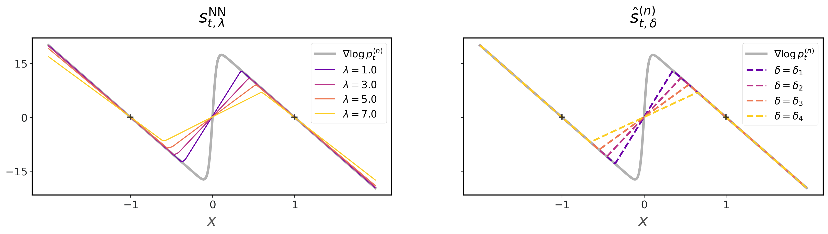
Figure 4: Similarities between NN-learned SF ($s^{\text{NN}}_{t,\lambda}$) under increasing strengths of regularization, $\lambda$ (Left) and the LA-PL SF ($\hat{s}^{(n)}_{t,\delta}$) with decreasing values of $\delta$ (Right) in the $d=1$, $n=2$ case with a fixed $t$. Details of the experiment setup are discussed in Section 6.1.

6.2 Experiment $2$: Denoising with Smoothed and NN-learned SF ($d=2$)

To validate the effect of score smoothing on the denoising dynamics and compare the different variants of smoothed SFs, we choose the setup in Section 5 with $d=2$ and $n=4$ and run the denoising dynamics (2) under three choices of the SF: (i) the ESF (${\bm{s}}_{t}=\nabla\log p^{(n)}_{t}$), (ii) the LA-PL SF (${\bm{s}}_{t}=\hat{{\bm{s}}}^{(n)}_{t,\delta_{t}}$ from (26)), and (iii) an NN-learned SF with $t$ as an input (${\bm{s}}_{t}={\bm{s}}^{\text{NN}}_{t}$).

All three processes are initialized at $t_{0}=0.02$ with the same marginal distribution ${\mathbf{x}}_{t_{0}}\sim p^{(n)}_{t_{0}}$ (and thus (i) is equivalent to an exact reversal of the forward process). The results are illustrated in Figure 5 and further details can be found in Appendix J.2.

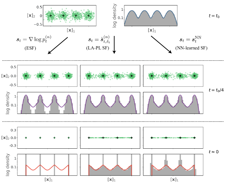
Figure 5: Results of the experiment described in Section 6.2, where each column shows the denoising process under one of three choices of the SF in the $d=2$, $n=4$ setting. Each process starts at $t=t_{0}=0.02$ with the marginal distribution $p^{(n)}_{t_{0}}$ and evolves backward-in-time according to the respective SF. At $t=t_{0}$, $t_{0}/4$ and $10^{-5}$, we plot (a) the samples from the denoising processes in ${\mathbb{R}}^{2}$ and (b) the density histograms (in log scale) of their projection onto the first dimension. In (b), the colored curves are the analytical predictions of $\hat{p}^{(n,t_{0})}_{t}$ (for $t=t_{0}$ and $t_{0}/4$) and $\tilde{p}^{(n,t_{0})}_{0}$ (for $t=10^{-5}$), with their formulas given in Appendix C.2. A direct comparison of the three SFs is given in Figures 7 - 9. A video animation of the three denoising processes and the evolution of the corresponding SFs can be found at this link.

Results.

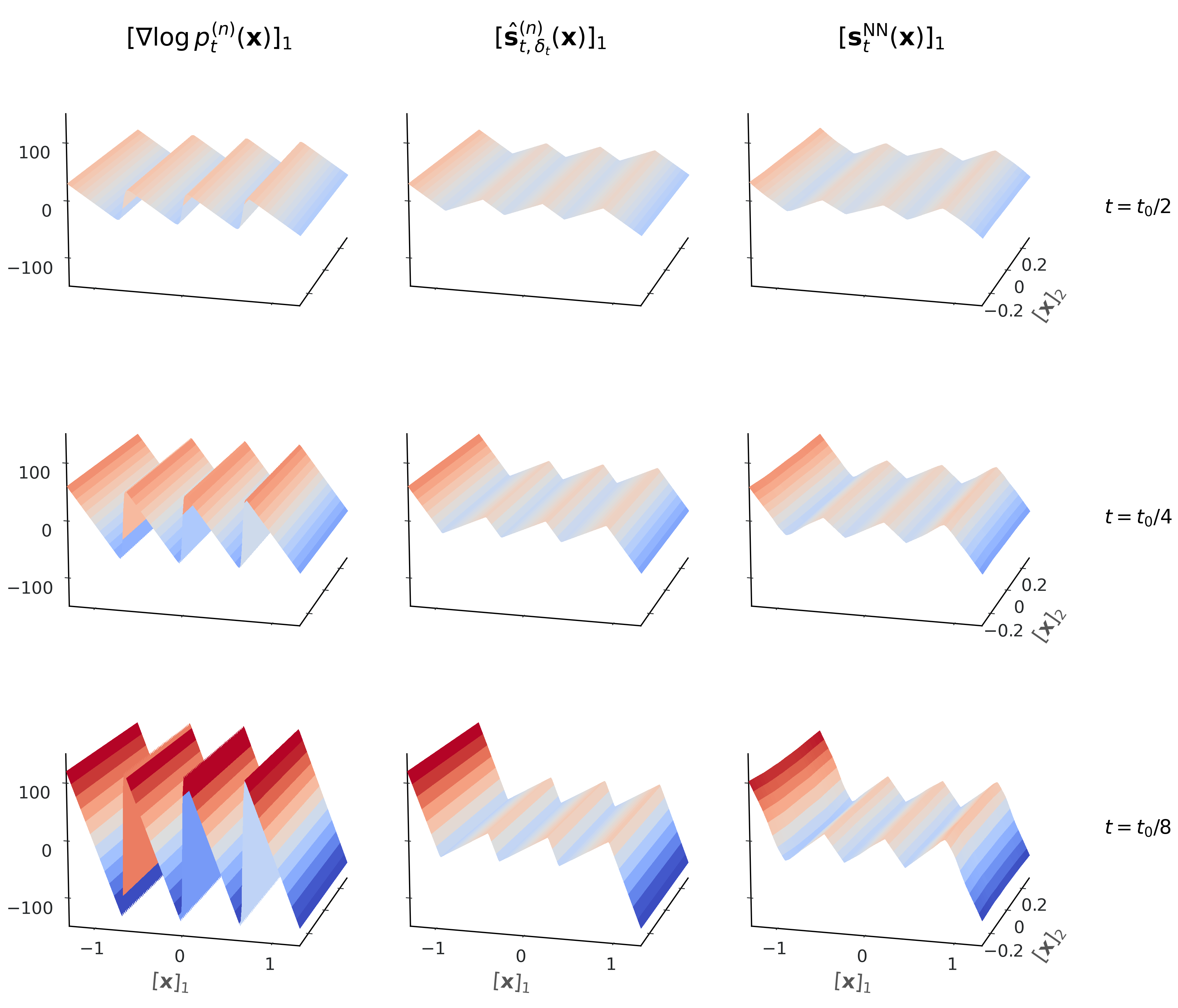
Figure 7: Comparing three SF variants from Experiment $2$ in their first (tangent) dimension at different $t$. We see a close proximity between the LA-PL SF and the NN-learned SF, both of which are smoother than the ESF especially at small $t$.

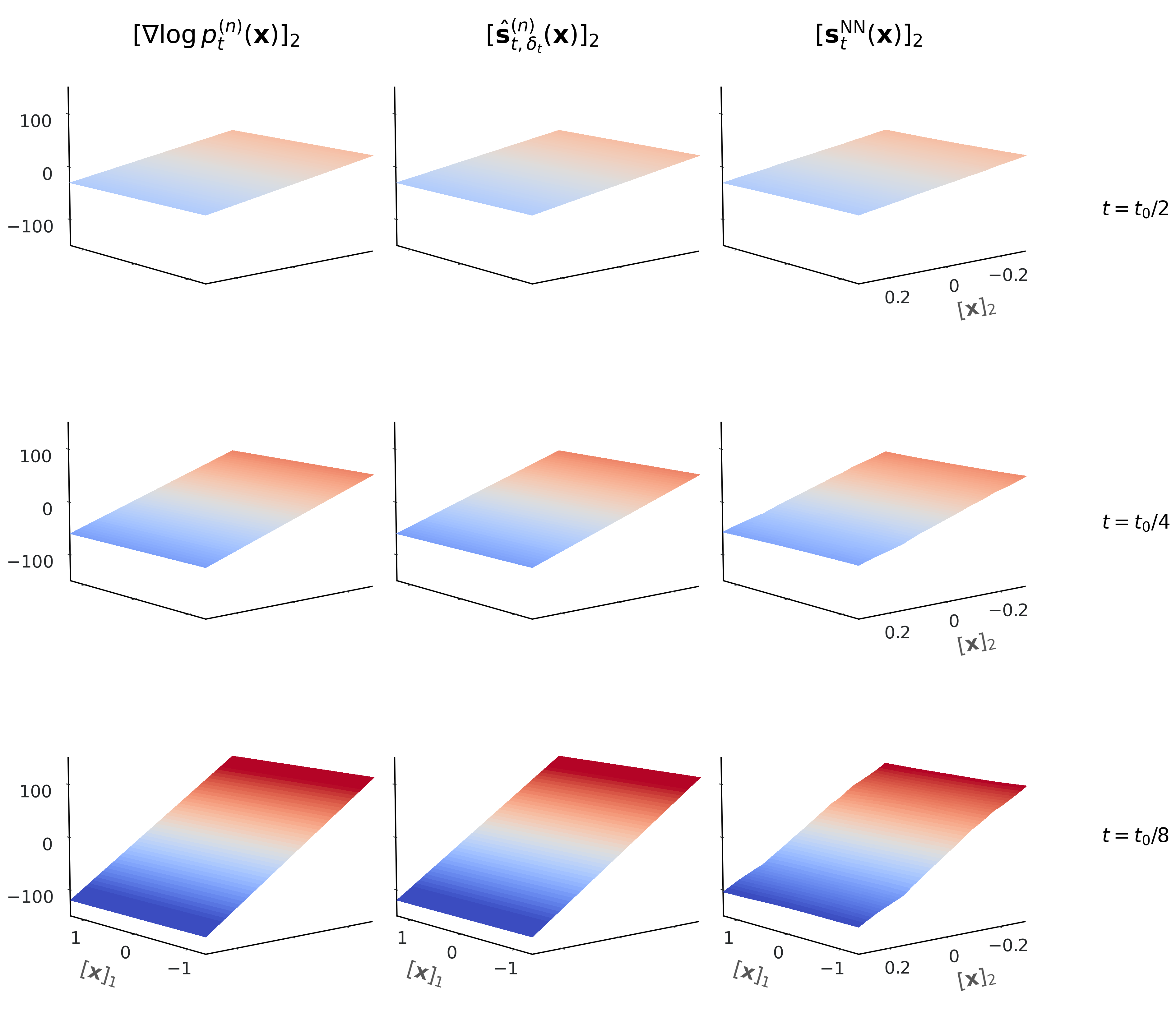
Figure 8: Comparing three SF variants from Experiment $2$ in their second (normal) dimension at different $t$. We see all three SF are relatively similar in the normal direction, except for a mild distortion of the NN-learned SF when $t$ is small and $[{\bm{x}}]_{2}$ is large (where $p^{(n)}_{t}$ has low density).

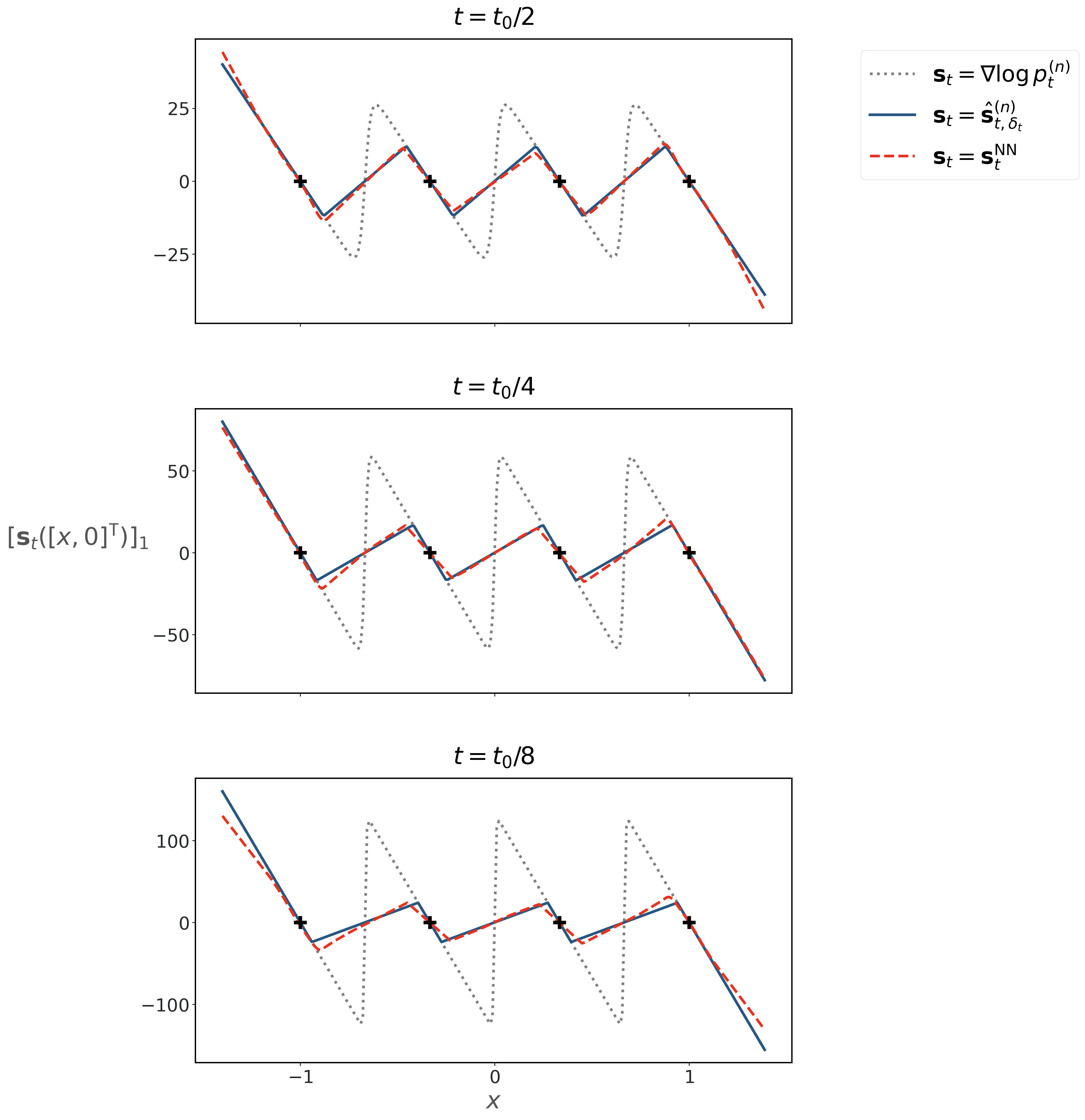
Figure 9: Comparing three SF variants from Experiment $2$ in their first (tangent) dimension at different $t$ when they are evaluated on the $[{\bm{x}}]_{1}$ axis. Again, we see a close proximity between the LA-PL SF and the NN-learned SF, both of which are smoother than the ESF.

We first observe that, in all three cases, the variance of the data distribution along the second dimension shrinks gradually to zero at a roughly similar rate as $t\to 0$, consistent with the theoretical argument in Section 5 that score smoothing does not interfere with the convergence in the normal direction. Meanwhile, in contrast with Column (i), where the variance along the first dimension shrinks to zero as well, we see in Column (ii) that the variance along the first dimension remains positive for all $t$, validating the interpolation effect caused by smoothing the ESF. Moreover, the density histograms in Column (ii) are closely matched by our analytical predictions of $\hat{p}^{(n,t_{0})}_{t}$ and $\tilde{p}^{(n,t_{0})}_{0}$ (the colored curves). Finally, we observe that Column (iii) is much closer to (ii) than (i) in terms of how the distribution (as well as the SF itself, as shown in Figures 7 - 9) evolves during denoising. This suggests that NN learning causes a similar smoothing effect on the SF and adds evidence that our analysis based on score smoothing is likely relevant for understanding how NN-based DMs avoid memorization.

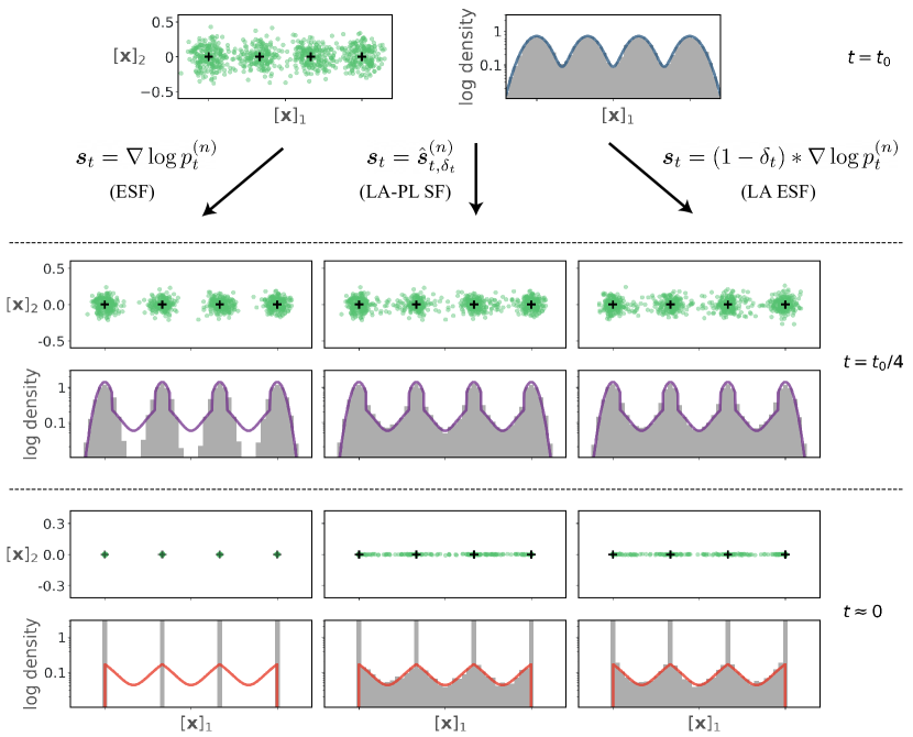
Figure 10: Additional results of Experiment $2$ discussed in Section 6.2. The only difference with Figure 5 is that the third column corresponds to driving the denoising dynamics with the locally-averaged ESF (${\bm{s}}_{t}=(1-\delta_{t})*\nabla\log p^{(n)}_{t}$). The fact that the last two columns are nearly identical gives evidence that the LA-PL SF is a good approximation to the locally-averaged ESF for the purpose of the denoising dynamics at small $t$.

In Figure 10, we also show that (ii) is nearly equivalent to the locally-averaged ESF (${\bm{s}}_{t}=(1-\delta_{t})*\nabla\log p^{(n)}_{t}$) for driving the denoising dynamics, which provides additional empirical justification for adopting the PL approximation at small $t$.

7 Related works

Generalization in DMs.

Several works have noted the transition from generalization to memorization behaviors in DMs when the model capacity increases relatively to the training set size (Gu et al.,, 2023; Yi et al.,, 2023; Carlini et al.,, 2023; Kadkhodaie et al.,, 2024; Li et al., 2024b, ). Using tools from statistical physics, Biroli et al., (2024) showed that the transition to memorization occurs in the crucial regime where $t$ is small relative to the training set sparsity, which is also the focus of our study.

To derive rigorous learning guarantees, one line of work showed that DMs can produce a distribution accurately given a good score estimator (Song et al., 2021a, ; Lee et al.,, 2022; De Bortoli,, 2022; Chen et al., 2023a, ; Chen et al., 2023c, ; Shah et al.,, 2023; Cole and Lu,, 2024; Benton et al.,, 2024; Huang et al., 2024a, ), which leaves open the question of how to estimate the SF of an underlying density from finite training data without overfitting. For score estimation, when the ground truth density or its SF belongs to certain function classes, prior works have constructed score estimators with guaranteed sample complexity (Block et al.,, 2020; Li et al.,, 2023; Zhang et al.,, 2024; Wibisono et al.,, 2024; Chen et al.,, 2024; Gatmiry et al.,, 2024; Boffi et al.,, 2025), including for scenarios where the data are supported on low-dimensional sub-manifolds (further discussed below). Unlike these approaches, which concern the estimation of densities from i.i.d. samples, our analysis does not assume a ground truth distribution. Based on a finite and fixed training set, our work focuses on the geometry of the SF when $t$ is small relative to the training set sparsity and elucidates how it determines the memorization behavior via an interplay with the denoising dynamics. For future work, it will be interesting to study the implication of score smoothing in the density estimation setting by potentially adapting our analysis to cases with randomly-sampled training data.

DMs and the manifold hypothesis.

An influential hypothesis is that high-dimensional real-world data often lie in low-dimensional sub-manifolds (Tenenbaum et al.,, 2000; Peyré,, 2009), and it has been argued that DMs can estimate their intrinsic dimensions (Stanczuk et al.,, 2024; Kamkari et al.,, 2024), learn manifold features in meaningful orders (Wang and Vastola,, 2023, 2024; Achilli et al.,, 2024), or perform subspace clustering implicitly (Wang et al.,, 2024). Under the manifold hypothesis, Pidstrigach, (2022); De Bortoli, (2022); Potaptchik et al., (2024); Huang et al., 2024b studied the convergence of DMs assuming a sufficiently good approximation to the true SF, while Oko et al., (2023); Chen et al., 2023b ; Azangulov et al., (2024) proved sample complexity guarantees for score estimation using NN models. In particular, prior works such as Chen et al., 2023b ; Wang and Vastola, (2024); Gao and Li, (2024); Ventura et al., (2024) have considered the decomposition of the SF into tangent and normal components. Our work is novel in showing how score smoothing can affect these two components differently: reducing the speed of convergence towards training data along the tangent direction (to avoid memorization) while preserving it along the normal direction (to ensure a convergence onto the subspace).

Score smoothing and regularization.

Aithal et al., (2024) showed empirically that NNs tend to learn smoother versions of the ESF and argued that this leads to a mode interpolation effect that explains model hallucination. Scarvelis et al., (2023) designed alternative closed-form DMs by smoothing the ESF, although the theoretical analysis therein is limited to showing that their smoothed SF is directed towards certain barycenters of the training data. Their work inspired our further theoretical analysis on how score smoothing affects the denoising dynamics and leads to a terminal distribution that interpolates the training data. In the context of image generation, Kamb and Ganguli, (2024) showed that imposing locality and equivariance to the score estimator allows the model to generalize better. In comparison, our work shows that the benefit of score regularization can manifest in more general settings via function smoothing.

Recent works including Wibisono et al., (2024); Baptista et al., (2025) considered other SF regularizers such as the empirical Bayes regularization (capping the magnitude in regions where $p^{(n)}_{t}$ is small) or Tikhonov regularization (constraining the norm averaged over $p^{(n)}_{t}$). In the linear subspace setting, these methods tend to reduce the magnitude of the SF in not only the tangent but also the normal directions, thus slowing down the convergence onto the subspace and resulting in a terminal distribution that still has a $d$-dimensional support. In contrast, as local averaging preserves the (linear) normal component, our smoothed score is less prone to this issue.

8 Conclusions and Limitations

Through theoretical analyses and numerical experiments, our work shows how score smoothing can enable the denoising dynamics to produce distributions on the training data subspace without fully memorizing the training set. Further, by showing connections between score smoothing and learning a score estimator with regularized NNs, our results shed light on an arguably core mechanism behind the ability of NN-based diffusion models to generalize and hallucinate. Additionally, viewing NN learning as just one way to achieve score smoothing, our work also motivates the exploration of alternative score estimators that facilitate generalization in DMs.

The present work focuses on a vastly simplified setup compared to real-world scenarios, and it would be valuable next steps to extend our theory to cases where training data are generally spaced, random or belonging to complex manifolds as well as to more general variants of DMs (De Bortoli et al.,, 2021; Albergo et al.,, 2023; Lipman et al.,, 2023; Liu et al.,, 2023). The connections between score smoothing and the implicit bias of NN training have also only been explored to a limited extent, especially in the higher-dimensional setting. Lastly, it will be useful to consider alternative forms of function smoothing as well as other ways regularization mechanisms beyond smoothing and better understand their interplay with the denoising dynamics.

Acknowledgment.

The author thanks Zhengjiang Lin, Pengning Chao, Pranjal Awasthi, Arnaud Doucet, Eric Vanden-Eijnden and Binxu Wang for valuable conversations and suggestions.

Appendix A Additional Notations

We use big-O notations only for denoting asymptotic relations as $t\to 0$. Specifically, for functions $f,g:{\mathbb{R}}_{+}\to{\mathbb{R}}_{+}$, we will write $f(t)=O(g(t))$ if $\exists t_{1},C>0$ (they may depend on other variables such as $\kappa$ and $\Delta$) such that $\forall t\in(0,t_{1})$, it holds that $f(t)\leq Cg(t)$. In addition, in several situations where $f$ decays exponentially fast in $1/t$ as $t\to 0$ but the exact exponent is not of much importance, we will simply write $f(t)=O(\exp(-C/t))$, which is intended to be interpreted as $\exists C>0$ such that $f(t)=O(\exp(-C/t))$ (and the value of $C$ can differ in different contexts).

Appendix B Connections Among the Different SF Variants

Figure 6: Different variants of the SF and their connections.

Appendix C Generalization to $n>2$

The analysis above can be generalized to the scenario where $S$ consists of $n>2$ points spaced uniformly on an interval $[-D,D]$, that is, $y_{k}\coloneqq 2(k-1)\Delta-D$ for $k\in[n]$, where $\Delta\coloneqq D/(n-1)=(y_{k+1}-y_{k})/2$. We additionally define $z_{k}\coloneqq y_{k}+\Delta=(y_{k}+y_{k+1})/2$ for $k\in[n-1]$.

C.1 Score Smoothing

In this case, we can still express the ESF as (6) except for replacing (7) by

$$\hat{x}^{(n)}_{t}(x)\coloneqq\frac{\sum_{k=1}^{n}y_{k}p_{\mathcal{N}}(x-y_{k},\sqrt{t})}{\sum_{k=1}^{n}p_{\mathcal{N}}(x-y_{k},\sqrt{t})}~,$$ (29)

and its PL approximation at small $t$ is now given by

$$\bar{s}^{(n)}_{t}(x)\coloneqq\begin{cases}(y_{1}-x)/t~,&\quad\text{ if }x\leq z_{1}~,\\ (y_{k}-x)/t~,&\quad\text{ if }x\in[z_{k-1},z_{k}]\text{ for }k\in\{2,...,n-1\}~,\\ (y_{n}-x)/t~,&\quad\text{ if }x\geq z_{n-1}~.\end{cases}$$ (30)

Moreover, the locally-averaged version of $\bar{s}^{(n)}_{t}$ can still be written via (11) for $\delta\in(0,\Delta)$, where we now define

$$\hat{s}^{(n)}_{t,\delta}(x)\coloneqq\begin{cases}(y_{1}-x)/t~,&~\text{ if }x\leq y_{1}+\delta~,\\ (y_{n}-x)/t~,&~\text{ if }x\geq y_{n-1}-\delta~,\\ (y_{k}-x)/t~,&~\text{ if }x\in[y_{k}-\delta,y_{k}+\delta],\exists k\in[n]~,\\ \delta/(\Delta-\delta)\cdot(x-z_{k})/t~,&~\text{ if }x\in[y_{k-1}+\delta,y_{k}-\delta],\exists k\in[n-1]~,\end{cases}$$ (31)

and it is not hard to show that Lemma 1 and Proposition 2 can be generalized to the following results, with their proofs given in Appendix D and E, respectively:

Lemma 7

For any fixed $\delta\in(0,\Delta]$, $\exists t_{1},C>0$ such that $\forall t\in(0,t_{1})$, it holds that

$$t\cdot{\mathbb{E}}_{x\sim p^{(n)}_{t}}\Big{[}\big{\|}\hat{s}^{(n)}_{t,\delta}(x)-((\Delta-\delta)*\tfrac{d}{dx}\log p^{(n)}_{t})(x)\big{\|}^{2}\Big{]}\leq C\exp(-\delta^{2}/(9t))~.$$ (32)

Proposition 8

Let $\delta_{t}=\kappa\sqrt{t}$ for some $\kappa>0$. Then $\exists t_{1},C>0$ such that $\forall t\in(0,t_{1})$,

$$\tfrac{n-1}{n}F(\kappa)-C\sqrt{t}\leq L^{(n)}_{t}[\hat{s}^{(n)}_{t,\delta_{t}}]\leq\tfrac{n-1}{n}F(\kappa)+C\sqrt{t}~,$$ (33)

where $t_{1}$ and $C$ depend only on $\kappa$ and $F$ is a function that strictly decreases from $1$ to $0$ on $[0,\infty)$.

C.2 Denoising Dynamics

The backward-in-time dynamics of (17) can also be solved analytically in a similar fashion, where (18) is replaced by

$$\phi_{s|t}(x)\coloneqq\begin{cases}\sqrt{\frac{s}{t}}(x-y_{1})+y_{1}~,&\text{ if }x\leq y_{1}+\delta_{t}~,\\ \sqrt{\frac{s}{t}}(x-y_{n})+y_{n}~,&\text{ if }x\geq y_{n}-\delta_{t}~,\\ \sqrt{\frac{s}{t}}(x-y_{k})+y_{k}~,&\text{ if }x\in[y_{k}-\delta_{t},y_{k}+\delta_{t}],\exists k\in\{2,...,n-1\}~,\\ \frac{\Delta-\delta_{s}}{\Delta-\delta_{t}}(x-z_{k})+z_{k}~,&\text{ if }x\in[y_{k}+\delta_{t},y_{k+1}-\delta_{t}],\exists k\in[n-1]~.\end{cases}$$ (34)

The formula (20) is then generalized to

$$\hat{p}^{(n,t_{0})}_{s}(x)=\begin{cases}\delta_{t}/\delta_{s}\cdot\hat{p}^{(n,t_{0})}_{t}(\delta_{t}/\delta_{s}\cdot x-(\delta_{t}-\delta_{s})/\delta_{s}\cdot y_{1})~,&\hskip-150.0pt\text{ if }x\leq y_{1}+\delta_{s}\\ \delta_{t}/\delta_{s}\cdot\hat{p}^{(n,t_{0})}_{t}(\delta_{t}/\delta_{s}\cdot x-(\delta_{t}-\delta_{s})/\delta_{s}\cdot y_{n})~,&\hskip-150.0pt\text{ if }x\geq y_{n}-\delta_{s}\\ \delta_{t}/\delta_{s}\cdot\hat{p}^{(n,t_{0})}_{t}(\delta_{t}/\delta_{s}\cdot x-(\delta_{t}-\delta_{s})/\delta_{s}\cdot y_{k})~,&\hskip-150.0pt\text{ if }x\in[y_{k}-\delta_{s},y_{k}+\delta_{s}]\\ (\Delta-\delta_{t})/(\Delta-\delta_{s})\cdot\hat{p}^{(n,t_{0})}_{t}((\Delta-\delta_{t})/(\Delta-\delta_{s})\cdot x+(\delta_{t}-\delta_{s})/(\Delta-\delta_{s})\cdot z_{k})~,\\ &\hskip-150.0pt\text{ if }x\in[y_{k}+\delta_{s},y_{k+1}-\delta_{s}]\end{cases}$$ (35)

When $s=0$, there is

$$\phi_{0|t}(x)=\begin{cases}(\Delta x-z_{k}\delta_{t})/(\Delta-\delta_{t})~,&\text{ if }x\in[y_{k}+\delta_{t},y_{k+1}-\delta_{t}],\exists k\in[n-1]~,\\ y_{\arg\min_{k}|y_{k}-x|}~,&\text{ otherwise. }\end{cases}$$ (36)

As $\phi_{0|t}(x)$ is invertible when restricted to $\cup_{k\in[n-1]}[y_{k}+\delta_{t},y_{k+1}-\delta_{t}]$, the terminal distribution can be decomposed as

$$\hat{p}^{(n,t_{0})}_{0}=\sum_{k=1}^{n}a_{k}\bm{\delta}_{y_{k}}+\Big{(}1-\sum_{k=1}^{n}a_{k}\bm{\delta}_{y_{k}}\Big{)}\tilde{p}^{(n,t_{0})}_{0}~,$$ (37)

where $\tilde{p}^{(n,t_{0})}_{0}$ is a probability distribution defined as

$$\tilde{p}^{(n,t_{0})}_{0}(x)=\begin{cases}(\Delta-\delta_{t})/\Delta\cdot\hat{p}^{(n,t_{0})}_{t}((\Delta-\delta_{t})/\Delta\cdot x+\delta_{t}/\Delta\cdot z_{k})~,&\quad\text{ if }x\in[y_{k},y_{k+1}]\\ 0~,&\quad\text{ otherwise}~.\end{cases}$$ (38)

and it holds for all $t\in(0,t_{0}]$ that

$$a_{k}=\begin{cases}{\mathbb{E}}_{{\mathbf{x}}\sim\hat{p}^{(n,t_{0})}_{t}}\big{[}\mathds{1}_{{\mathbf{x}}\geq-D+\delta_{t}}\big{]}~,&\quad\text{if }k=1~,\\ {\mathbb{E}}_{{\mathbf{x}}\sim\hat{p}^{(n,t_{0})}_{t}}\big{[}\mathds{1}_{{\mathbf{x}}\geq D-\delta_{t}}\big{]}~,&\quad\text{if }k=n~,\\ {\mathbb{E}}_{{\mathbf{x}}\sim\hat{p}^{(n,t_{0})}_{t}}\big{[}\mathds{1}_{y_{k}-\delta_{t}\leq{\mathbf{x}}\leq y_{k}+\delta_{t}}\big{]}~,&\quad\text{if }k\in\{2,...,n-1\}~.\end{cases}$$ (39)

C.3 Higher Dimensions

Thanks to the decoupling across dimensions, under the definition of local averaging over centered cubes (24), the LA-PL SF takes the same form as (26) and the denoising dynamics associated with it also follows (27) and (28). Hence, Proposition 6 still holds except with (18) - (21) replaced by (34), (36), (35), and (38), respectively.

Appendix D Proof of Lemma 1

Below we prove Lemma 7, which generalizes Lemma 1 to the case where $n>2$.

We write $w=\Delta-\delta$. By the definition of $p^{(n)}_{t}$, it suffices to show that $\forall k\in[n]$,

$$\int|(w*\tfrac{d}{dx}\log p^{(n)}_{t})(x)-(w*\bar{s}^{(n)}_{t})(x)|^{2}p_{\mathcal{N}}(x-y_{k};\sqrt{t})dx=O(\exp(-\delta^{2}/(9t)))~.$$ (40)

Consider any $k\in[n]$. The left-hand-side above can be rewritten as

$$\begin{split}&~\int_{-\infty}^{\infty}\left|\frac{1}{2w}\int_{x-w}^{x+w}\tfrac{d}{dx}\log p^{(n)}_{t}(x^{\prime})dx^{\prime}-\frac{1}{2w}\int_{x-w}^{x+w}\bar{s}^{(n)}_{t}(x^{\prime})dx^{\prime}\right|^{2}p_{\mathcal{N}}(x-y_{k};\sqrt{t})dx\\ =&~\int_{-\infty}^{\infty}\left|\frac{1}{2w}\int_{x-w}^{x+w}\left(\tfrac{d}{dx}\log p^{(n)}_{t}(x^{\prime})-\bar{s}^{(n)}_{t}(x^{\prime})\right)dx^{\prime}\right|^{2}p_{\mathcal{N}}(x-y_{k};\sqrt{t})dx\\ \leq&~\int_{-\infty}^{\infty}\frac{1}{2w}\int_{x-w}^{x+w}\left|\tfrac{d}{dx}\log p^{(n)}_{t}(x^{\prime})-\bar{s}^{(n)}_{t}(x^{\prime})\right|^{2}dx^{\prime}p_{\mathcal{N}}(x-y_{k};\sqrt{t})dx\\ =&~\int_{-\infty}^{\infty}\left|\tfrac{d}{dx}\log p^{(n)}_{t}(x^{\prime})-\bar{s}^{(n)}_{t}(x^{\prime})\right|^{2}\left(\frac{1}{2w}\int_{x^{\prime}-w}^{x^{\prime}+w}p_{\mathcal{N}}(x-y_{k};\sqrt{t})dx\right)dx^{\prime}\end{split}$$ (41)

We decompose the outer integral into three intervals and bound them separately. First, when $x\geq y_{k}+\frac{1}{2}(\Delta+w)>y_{k}+w$, there is $\sup_{x\in[x^{\prime}-w,x^{\prime}+w]}p_{\mathcal{N}}(x-y_{k};\sqrt{t})\leq p_{\mathcal{N}}(x^{\prime}-y_{k}-w;\sqrt{t})$. Hence, also noticing that $|\tfrac{d}{dx}\log p^{(n)}_{t}(x)|,|\bar{s}^{(n)}_{t}(x)|\leq(|x|+2D)/t$, we obtain that

$$\begin{split}&~\int_{y_{k}+\frac{1}{2}(\Delta+w)}^{\infty}\left|\tfrac{d}{dx}\log p^{(n)}_{t}(x^{\prime})-\bar{s}^{(n)}_{t}(x^{\prime})\right|^{2}\left(\frac{1}{2w}\int_{x^{\prime}-w}^{x^{\prime}+w}p_{\mathcal{N}}(x-y_{k};\sqrt{t})dx\right)dx^{\prime}\\ \leq&~\frac{1}{\sqrt{2\pi t}}\int_{y_{k}+\frac{1}{2}(\Delta+w)}^{\infty}\left|\tfrac{d}{dx}\log p^{(n)}_{t}(x^{\prime})-\bar{s}^{(n)}_{t}(x^{\prime})\right|^{2}\exp\left(-\frac{(x^{\prime}-y_{k}-w)^{2}}{2t}\right)dx^{\prime}\\ \leq&~\frac{1}{\sqrt{2\pi t}}\int_{y_{k}+\frac{1}{2}(\Delta+w)}^{\infty}\frac{4(|x^{\prime}|+2D)^{2}}{t^{2}}\exp\left(-\frac{(x^{\prime}-y_{k}-w)^{2}}{2t}\right)dx^{\prime}\\ \leq&~\frac{1}{\sqrt{2\pi t}}\int_{y_{k}+\frac{1}{2}(\Delta+w)}^{\infty}\frac{4(|x^{\prime}-y_{k}-w|+4D)^{2}}{t^{2}}\exp\left(-\frac{(x^{\prime}-y_{k}-w)^{2}}{2t}\right)dx^{\prime}\\ \leq&~\frac{8}{\sqrt{2\pi t^{3}}}\int_{y_{k}+\frac{1}{2}(\Delta+w)}^{\infty}\left(\left(\frac{x^{\prime}-y_{k}-w}{\sqrt{t}}\right)^{2}+\frac{16D^{2}}{t}\right)\exp\left(-\frac{(x^{\prime}-y_{k}-w)^{2}}{2t}\right)dx^{\prime}\\ =&~\frac{8}{\sqrt{2\pi t^{3}}}\int_{\frac{\delta}{2\sqrt{t}}}^{\infty}\left((\tilde{x})^{2}+\frac{16D^{2}}{t}\right)\exp\left(-\frac{(\tilde{x})^{2}}{2}\right)d\tilde{x}\\ \leq&~\frac{8}{\sqrt{2\pi t^{3}}}\left(\bigg{(}\frac{16D^{2}}{t}+1\bigg{)}\sqrt{\frac{\pi}{2}}+\frac{\delta}{2\sqrt{t}}\right)\exp\left(-\frac{\delta^{2}}{8t}\right)=O\left(\exp\left(-\frac{\delta^{2}}{9t}\right)\right)~,\end{split}$$ (42)

where for the last inequality we use Lemma 9 below.

A similar bound can be derived when the range of the outer integral is changed to between $-\infty$ and $y_{k}-\frac{1}{2}(\Delta+w)$.

Next, suppose $x\in[y_{k}-\frac{1}{2}(\Delta+w),y_{k}+\frac{1}{2}(\Delta+w)]$, which means that $|x-y_{k}|\leq\frac{1}{2}(\Delta+w)$ while $|x-y_{l}|\geq\frac{3}{2}\Delta-\frac{1}{2}w$ for $l\neq k$. Thus, it holds for any $l\neq k$ that

$$\begin{split}\frac{p_{\mathcal{N}}(x-y_{k};\sqrt{t})}{p_{\mathcal{N}}(x-x_{l};\sqrt{t})}=&~\exp\left(-\frac{|x-y_{k}|^{2}-|x-x_{l}^{2}|}{2t}\right)\geq\exp\left(\frac{\Delta\delta}{t}\right)\end{split}$$ (43)

Hence, writing $q_{t,k}(x)\coloneqq\frac{p_{\mathcal{N}}(x-y_{k};\sqrt{t})}{\sum_{l=1}^{n}p_{\mathcal{N}}(x-x_{l};\sqrt{t})}$, there is $q_{t,k}(x)\geq 1-(n-1)\exp\left(-\frac{\Delta\delta}{t}\right)$ and for $l\neq k$, $q_{t,l}(x)<\exp\left(-\frac{\Delta\delta}{t}\right)$. Therefore,

$$\begin{split}\left|\tfrac{d}{dx}\log p^{(n)}_{t}(x)-\bar{s}^{(n)}_{t}(x)\right|\leq&~\frac{|(q_{t,k}(x)-1)y_{k}|+\sum_{l\neq k}|q_{t,k}(x)y_{k}|}{t}\\ \leq&~\frac{2(n-1)D}{t}\exp\left(-\frac{\Delta\delta}{t}\right)=O\left(t^{-1}\exp\left(-\frac{\Delta\delta}{t}\right)\right)~.\end{split}$$ (44)

Since $\frac{1}{2w}\int_{x^{\prime}-w}^{x^{\prime}+w}p_{\mathcal{N}}(x-y_{k};\sqrt{t})dx\leq\frac{1}{\sqrt{2\pi t}}$ for any $x^{\prime}$, we then have

$$\begin{split}&~\int_{y_{k}-\frac{1}{2}(\Delta+w)}^{y_{k}+\frac{1}{2}(\Delta+w)}\left|\tfrac{d}{dx}\log p^{(n)}_{t}(x^{\prime})-\bar{s}^{(n)}_{t}(x^{\prime})\right|^{2}\left(\frac{1}{2w}\int_{x^{\prime}-w}^{x^{\prime}+w}p_{\mathcal{N}}(x-y_{k};\sqrt{t})dx\right)dx^{\prime}\\ \leq&~\frac{\Delta+w}{\sqrt{2\pi t}}\sup_{y_{k}-\frac{1}{2}(\Delta+w)\leq x^{\prime}\leq y_{k}+\frac{1}{2}(\Delta+w)}\left|\tfrac{d}{dx}\log p^{(n)}_{t}(x^{\prime})-\bar{s}^{(n)}_{t}(x^{\prime})\right|^{2}\\ =&~O\left(t^{-3}\exp\left(-\frac{2\Delta\delta}{t}\right)\right)\end{split}$$ (45)

Combining (42) with (45) yields the desired result.

$\square$

Lemma 9

For $u\geq 0$,

$$\int_{u}^{\infty}e^{-x^{2}/2}dx\leq ~\sqrt{\frac{\pi}{2}}e^{-u^{2}/2}$$ (46)

$$\int_{u}^{\infty}x^{2}e^{-x^{2}/2}dx\leq ~\left(\sqrt{\frac{\pi}{2}}+u\right)e^{-u^{2}/2}$$ (47)

Proof of Lemma 9: It known (e.g., Chang et al., 2011) that

$$\int_{u}^{\infty}e^{-x^{2}}dx\leq\frac{\sqrt{\pi}}{2}e^{-u^{2}}~,$$ (48)

from which (46) can be obtained by a simple change-of-variable.

Next, using integration-by-parts, we obtain that

$$\begin{split}\int_{a}^{b}x^{2}e^{-x^{2}/2}dx=&~x(-e^{-x^{2}/2})\big{|}_{a}^{b}-\int_{a}^{b}1\cdot(-e^{-\frac{x^{2}}{2}})dx\\ =&~(ae^{-a^{2}/2}-be^{-b^{2}/2})+\int_{a}^{b}e^{-x^{2}/2}dx\end{split}$$ (49)

Hence,

$$\begin{split}\int_{u}^{\infty}x^{2}e^{-x^{2}/2}dx\leq&~\int_{u}^{\infty}e^{-x^{2}/2}dx+ue^{-u^{2}/2}\\ \leq&~\left(\sqrt{\frac{\pi}{2}}+u\right)e^{-u^{2}/2}\end{split}$$ (50)

$\square$

Appendix E Proof of Proposition 2

Below we prove Proposition 8, which generalizes Proposition 2 to the case where $n>2$.

In light of Lemma 1, we only need to show that

$$t\int_{-\infty}^{\infty}|\hat{s}^{(n)}_{t,\delta_{t}}(x)-\bar{s}^{(n)}_{t}(x)|^{2}p^{(n)}_{t}(x)dx=\frac{n-1}{n}F(\kappa)+O(\sqrt{t})~.$$ (51)

By the definition of $p^{(n)}_{t}$, we can first evaluate the integral with respect to the density $p_{\mathcal{N}}(x-y_{k};\sqrt{t})$ for each $k\in[n]$ separately and then sum them up. We define

$$y_{k,-}=\begin{cases}-\infty~,&~\text{ if }k=1\\ y_{k}-\delta_{t}~,&~\text{ otherwise}\end{cases},\qquad y_{k,+}=\begin{cases}\infty~,&~\text{ if }k=n\\ y_{k}+\delta_{t}~,&~\text{ otherwise}\end{cases}$$ (52)

By construction, $\hat{s}^{(n)}_{t,\delta_{t}}$ is a PL function whose slope is changed only at each $y_{k,-}$ and $y_{k,+}$.

Let us fix a $k\in[n]$. Since $\hat{s}^{(n)}_{t,\delta_{t}}(x)=\bar{s}^{(n)}_{t}(x)$ when $x\in[y_{k,-},y_{k,+}]$, we only need to estimate the difference between the two outside of $[y_{k,-},y_{k,+}]$.

We first consider the interval $(y_{k,+},y_{k}+\Delta]=(y_{k}+\delta_{t},y_{k}+\Delta]$ when $k\in\{1,...,n-1\}$, on which it holds that

$$\hat{s}^{(n)}_{t,\delta_{t}}(x)-\bar{s}^{(n)}_{t}(x)=\frac{\Delta}{t}\cdot\frac{x-(y_{k}+\delta_{t})}{\Delta-\delta_{t}}~,$$ (53)

by the piecewise-linearity of the two functions. Hence,

$$\begin{split}&~t\int_{y_{k}+\delta_{t}}^{y_{k}+\Delta}|\hat{s}^{(n)}_{t,\delta_{t}}(x)-\bar{s}^{(n)}_{t}(x)|^{2}p_{\mathcal{N}}(x-y_{k};\sqrt{t})dx\\ =&~\left(\frac{\Delta}{\Delta-\delta_{t}}\right)^{2}\int_{y_{k}+\delta_{t}}^{y_{k}+\Delta}\left|\frac{x-y_{k}}{\sqrt{t}}-\frac{\delta_{t}}{\sqrt{t}}\right|^{2}p_{\mathcal{N}}(x-y_{k};\sqrt{t})dx\\ =&~\left(\frac{\Delta}{\Delta-\delta_{t}}\right)^{2}\bigg{(}\int_{y_{k}+\delta_{t}}^{\infty}\left|\frac{x-y_{k}}{\sqrt{t}}-\kappa\right|^{2}p_{\mathcal{N}}(x-y_{k};\sqrt{t})dx\\ &\hskip 50.0pt-\int_{y_{k}+\Delta}^{\infty}\left|\frac{x-y_{k}}{\sqrt{t}}-\kappa\right|^{2}p_{\mathcal{N}}(x-y_{k};\sqrt{t})dx\bigg{)}\end{split}$$ (54)

Note that by a change-of-variable $\tilde{x}\leftarrow(x-y_{k})/\sqrt{t}$, we obtain that

$$\begin{split}\int_{y_{k}+\delta_{t}}^{\infty}\left|\frac{x-y_{k}}{\sqrt{t}}-\kappa\right|^{2}p_{\mathcal{N}}(x-y_{k};\sqrt{t})dx=\frac{1}{2}F(\kappa)~,\end{split}$$ (55)

where we define

$$F(\kappa)\coloneqq 2\int_{\kappa}^{\infty}|u-\kappa|^{2}p_{\mathcal{N}}(u;1)du$$ (56)

It is straightforward to see that, as $\kappa$ increases from $0$ to $\infty$, $F$ strictly decreases from $1$ to $0$. Therefore,

$$\begin{split}&~t\int_{y_{k}+\delta_{t}}^{y_{k}+\Delta}|\hat{s}^{(n)}_{t,\delta_{t}}(x)-\bar{s}^{(n)}_{t}(x)|^{2}p_{\mathcal{N}}(x-y_{k};\sqrt{t})dx\\ =&~\left(\frac{\Delta}{\Delta-\delta_{t}}\right)^{2}\left(\frac{1}{2}F(\kappa)-\int_{\Delta/\sqrt{t}}^{\infty}\left|u-\kappa\right|^{2}p_{\mathcal{N}}(u;1)dx\right)\\ =&~\frac{1}{2}F(\kappa)+O(\sqrt{t})\end{split}$$ (57)

Next, we consider the interval $[y_{k}+\Delta,\infty)$, in which we have

$$|\hat{s}^{(n)}_{t,\delta_{t}}(x)-\bar{s}^{(n)}_{t}(x)|\leq\frac{\Delta}{t}~.$$ (58)

Thus,

$$\begin{split}t\int_{y_{k}+\Delta}^{\infty}|\hat{s}^{(n)}_{t,\delta_{t}}(x)-\bar{s}^{(n)}_{t}(x)|^{2}p_{\mathcal{N}}(x-y_{k};\sqrt{t})dx\leq&~t\int_{y_{k}+\Delta}^{\infty}\left|\frac{\Delta}{t}\right|^{2}p_{\mathcal{N}}(x-y_{k};\sqrt{t})dx\\ =&~\frac{\Delta^{2}}{t}\int_{\Delta/\sqrt{t}}^{\infty}p_{\mathcal{N}}(u;1)du\\ =&~O\left(t^{-1}\exp\bigg{(}-\frac{\Delta^{2}}{2t}\bigg{)}\right)\end{split}$$ (59)

Hence, we have

$$t\int_{y_{k}+\delta_{t}}^{\infty}|\hat{s}^{(n)}_{t,\delta_{t}}(x)-\bar{s}^{(n)}_{t}(x)|^{2}p_{\mathcal{N}}(x-y_{k};\sqrt{t})dx=\frac{1}{2}F(\kappa)+O(\sqrt{t})~.$$ (60)

Similarly, for $k\in\{2,...,n\}$, we can show that

$$t\int_{-\infty}^{y_{k}-\delta_{t}}|\hat{s}^{(n)}_{t,\delta_{t}}(x)-\bar{s}^{(n)}_{t}(x)|^{2}p_{\mathcal{N}}(x-y_{k};\sqrt{t})dx=\frac{1}{2}F(\kappa)+O(\sqrt{t})~.$$ (61)

Thus, there is

$$\begin{split}&t\int_{-\infty}^{\infty}|\hat{s}^{(n)}_{t,\delta_{t}}(x)-\bar{s}^{(n)}_{t}(x)|^{2}p_{\mathcal{N}}(x-y_{k};\sqrt{t})dx\\ =&~\begin{cases}F(\kappa)+O(\sqrt{t})~,&\quad\text{ if }k\in\{2,...,n-1\}\\ \frac{1}{2}F(\kappa)+O(\sqrt{t})~,&\quad\text{ if }k=1\text{ or }n~.\end{cases}\end{split}$$ (62)

Summing them together, we get that

$$t\int_{-\infty}^{\infty}|\hat{s}^{(n)}_{t,\delta_{t}}(x)-\bar{s}^{(n)}_{t}(x)|^{2}p^{(n)}_{t}(x)dx=\frac{n-1}{n}F(\kappa)+O(\sqrt{t})~.$$ (63)

This proves the proposition.

$\square$

Appendix F Proof of Proposition 3

The first claim is a straightforward consequence of Proposition 8: when $t$ is small enough (with threshold dependent on $\kappa$), there is

$$L^{(n)}_{t}[\hat{s}^{(n)}_{t,\delta_{t}}]\leq\frac{n-1}{n}F(\kappa)+C\sqrt{t}<F(\kappa)\leq F(F^{-1}(\epsilon))=\epsilon~.$$ (64)

Next we consider the second claim. On one hand, it is easy to compute that

$$\begin{split}R[\hat{s}^{(n)}_{t,\delta_{t}}]=&~\sum_{k=1}^{n-1}2\left(\frac{\delta_{t}}{t(\Delta-\delta_{t})}+\frac{1}{t}\right)=2(n-1)\frac{\Delta}{t(\Delta-\delta_{t})}\end{split}$$ (65)

On the other hand, let $f$ be any function on ${\mathbb{R}}$ that belongs to the feasible set of the minimization problem (16), meaning that $f$ is twice differentiable except on a set of measure zero and $L^{(n)}_{t}[f]<\epsilon$. Define $\epsilon_{k}\coloneqq t\int_{-\infty}^{\infty}|f(x)-\tfrac{d}{dx}\log p^{(n)}_{t}(x)|^{2}p_{\mathcal{N}}(x-y_{k};\sqrt{t})dx$ for each $k\in[n]$. By the definition of $p^{(n)}_{t}$, we then have $\sum_{k=1}^{n}\epsilon_{k}<n\epsilon$. If we consider a change-of-variable $\tilde{x}=(x-y_{k})/\sqrt{t}$ and define $\tilde{f}_{k}(\tilde{x})\coloneqq\sqrt{t}f(y_{k}+\sqrt{t}\tilde{x})$, there is

$$\begin{split}\int_{y_{k}-\Delta}^{y_{k}+\Delta}|f(x)-\bar{s}^{(n)}_{t}(x)|^{2}p_{\mathcal{N}}(x-y_{k};\sqrt{t})dx=&~\int_{y_{k}-\Delta}^{y_{k}+\Delta}\Big{|}f(x)-\frac{y_{k}-x}{t}\Big{|}^{2}p_{\mathcal{N}}(x-y_{k};\sqrt{t})dx\\ =&~t^{-1}\int_{-\Delta/\sqrt{t}}^{\Delta/\sqrt{t}}|\tilde{f}_{k}(\tilde{x})+\tilde{x}|^{2}p_{\mathcal{N}}(\tilde{x};1)d\tilde{x}~.\end{split}$$ (66)

Hence, using (40) with $\delta=\Delta$, we obtain that

$$\begin{split}\int_{-\Delta/\sqrt{t}}^{\Delta/\sqrt{t}}|\tilde{f}_{k}(\tilde{x})+\tilde{x}|^{2}p_{\mathcal{N}}(\tilde{x};1)d\tilde{x}\leq&~t\int_{-\infty}^{\infty}|f(x)-\bar{s}^{(n)}_{t}(x)|^{2}p_{\mathcal{N}}(x-y_{k};\sqrt{t})dx\\ \leq&~t\int_{-\infty}^{\infty}|f(x)-\tfrac{d}{dx}\log p^{(n)}_{t}(x)|^{2}p_{\mathcal{N}}(x-y_{k};\sqrt{t})dx\\ &~+t\int_{-\infty}^{\infty}\big{|}\tfrac{d}{dx}\log p^{(n)}_{t}(x)-\bar{s}^{(n)}_{t}(x)\big{|}^{2}p_{\mathcal{N}}(x-y_{k};\sqrt{t})dx\\ \leq&~\epsilon_{k}+O(\exp(-\Delta^{2}/(9t)))~.\end{split}$$ (67)

Thus, for $t$ small enough such that $\sqrt{t}<\Delta/3$, we can apply Lemma 10 from below to $\tilde{f}_{k}$, from which we obtain (after reversing the change-of-variable) that

$$\begin{split}\hskip 20.0pt\inf_{x\in[y_{k}-1.5\sigma,y_{k}+1.5\sigma]\setminus N}f^{\prime}(x)\leq&~(-1+2\sqrt{\epsilon_{k}})/t+O(\exp(-\Delta^{2}/(10t)))\\ \inf_{x\in[y_{k}+1.5\sigma,y_{k}+3\sigma]}f(x)\leq&~-0.5\\ \sup_{x\in[y_{k}-3\sigma,y_{k}-1.5\sigma]}f(x)\geq&~0.5~.\end{split}$$ (68)

Hence, $\exists a_{k}\in[y_{k}-1.5\sigma,y_{k}+1.5\sigma]\setminus N$, $b_{k,+}\in[y_{k}+1.5\sigma,y_{k}+3\sigma]$ and $b_{k,-}\in[y_{k}-3\sigma,y_{k}-1.5\sigma]$ such that $f^{\prime}(a_{k})\leq(-1+2\sqrt{\epsilon_{k}})/t+O(\exp(-\Delta^{2}/(10t)))$, $f(b_{k,+})\leq 0$ and $f(b_{k,-})\geq 0$. Furthermore, for $t$ small enough such that $\sqrt{t}<\Delta/6$, there is $b_{k,+}<b_{k+1,-}$ for $k\in[n-1]$, and hence by the fundamental theorem of calculus, $\exists c_{k}\in[b_{k,+},b_{k+1,-}]$ such that $f^{\prime}(c_{k})\geq 0$.

Now, we focus on the sequence of points, $a_{1}<c_{1}<a_{2}<...<c_{n-1}<a_{n}$. By the fundamental theorem of calculus and the fact that $f$ is twice differentiable except for on a finite set, there is

$$\int_{a_{k}}^{c_{k}}|f^{\prime\prime}(x)|dx\geq ~|f^{\prime}(c_{k})-f^{\prime}(a_{k})|\geq(1-2\sqrt{\epsilon_{k}})/t-O(\exp(-\Delta^{2}/(10t)))$$

$$\int_{c_{k}}^{a_{k+1}}|f^{\prime\prime}(x)|dx\geq ~|f^{\prime}(a_{k+1})-f^{\prime}(c_{k})|\geq(1-2\sqrt{\epsilon_{k+1}})/t-O(\exp(-\Delta^{2}/(10t)))$$

and hence it is clear that

$$\begin{split}R[f]=\int_{-\infty}^{\infty}|f^{\prime\prime}(x)|dx\geq&~\sum_{k=1}^{n-1}|f^{\prime}(c_{k})-f^{\prime}(a_{k})|+\sum_{k=1}^{n-1}|f^{\prime}(a_{k+1})-f^{\prime}(c_{k})|\\ \geq&~2\Big{(}n-1-\sum_{k=1}^{n}2\sqrt{\epsilon_{k}}\Big{)}/t-O(\exp(-\Delta^{2}/(10t)))\\ \geq&~2(n-1-2n\sqrt{\epsilon})/t-O(\exp(-\Delta^{2}/(10t)))~.\end{split}$$ (69)

Therefore, for $0<\epsilon<0.015$, as $n\geq 2$, it holds for $t$ sufficiently small that

$$\begin{split}\frac{R[\hat{s}^{(n)}_{t,\delta_{t}}]}{R[f]}\leq&~\frac{(n-1)\Delta}{(n-1-2n\sqrt{\epsilon})(\Delta-\delta_{t})-O(\exp(-\Delta^{2}/(10t)))}\\ \leq&~1+7.9\sqrt{\epsilon}+O(\sqrt{t})~,\end{split}$$ (70)

which is bounded by $1+8\sqrt{\epsilon}$. Since this holds for any $f$ in the feasible set, it also holds when the denominator on the left-hand-side is replaced by the infimum, $r_{t,\epsilon}^{*}$.

$\square$

Lemma 10

Suppose $f$ is twice differentiable on ${\mathbb{R}}$ except on a set $N$ of measure zero and $\int_{-3}^{3}|x+f(x)|^{2}p_{\mathcal{N}}(x;1)dx<\epsilon$ with $0<\epsilon<0.03$. Then we have

$$\inf_{x\in[-1.5,~1.5]\setminus N}f^{\prime}(x)\leq ~-1+2\sqrt{\epsilon}$$ (71)

$$\inf_{x\in[1.5,~3]}f(x)\leq ~-0.5$$ (72)

$$\sup_{x\in[-1.5,~-3]}f(x)\geq ~0.5$$ (73)

Proof of Lemma 10: We first prove (71) by supposing for contradiction that $\inf_{x\in[-1.5,~1.5]\setminus N}f^{\prime}(x)=-1+k_{\Delta}$ with $k_{\Delta}>2\sqrt{\epsilon}$. By the fundamental theorem of calculus, this means that the function $x+f(x)$ is monotonically increasing with slope at least $k_{\Delta}$ on $[-1.5,1.5]$. Hence, there exists $x_{1}\in\mathbb{R}$ such that $|x+f(x)|>k_{\Delta}|x-x_{1}|$ for $x\in[-1.5,1.5]$. Therefore,

$$\begin{split}\int_{-\infty}^{\infty}|x+f(x)|^{2}p_{\mathcal{N}}(x;1)dx\geq&~\int_{-1.5}^{1.5}|x+f(x)|^{2}p_{\mathcal{N}}(x;1)dx\\ \geq&~(k_{\Delta})^{2}\int_{-1.5}^{1.5}|x-x_{1}|^{2}p_{\mathcal{N}}(x;1)dx\\ =&~(k_{\Delta})^{2}\int_{-1.5}^{1.5}(x^{2}+2xx_{1}+(x_{1})^{2})p_{\mathcal{N}}(x;1)dx\\ \geq&~(k_{\Delta})^{2}\int_{-1.5}^{1.5}x^{2}p_{\mathcal{N}}(x;1)dx\\ >&~0.25(k_{\Delta})^{2}>\epsilon~,\end{split}$$ (74)

which shows a contradiction.

Next, we prove (72) by supposing for contradiction that $\inf_{x\in[1.5,~3]\setminus N}f(x)>-0.5$, in which case it holds that $\inf_{1.5\leq x\leq 3}|f(x)+x|>1$, and hence

$$\begin{split}\int_{-\infty}^{\infty}|x+f(x)|^{2}p_{\mathcal{N}}(x;1)dx\geq&~\int_{1.5}^{3}|x+f(x)|^{2}p_{\mathcal{N}}(x;1)dx\\ \geq&~\int_{1.5}^{3}p_{\mathcal{N}}(x;1)dx\\ >&~0.03>\epsilon\end{split}$$ (75)

which shows a contradiction. A similar argument can be used to prove (73).

$\square$

Appendix G Alternative Definition of Local Averaging in Higher Dimensions

Given a compact set of vectors, $A\subseteq{\mathbb{R}}^{d}$, we define its element with minimum Euclidean norm as

$$\gamma(A)\coloneqq\begin{cases}\arg\min_{{\bm{v}}\in A}\|{\bm{v}}\|_{2}~,&\quad\text{ if }\arg\min_{{\bm{v}}\in A}\|{\bm{v}}\|_{2}\text{ is unique}\\ {\bm{0}}~,&\quad\text{ otherwise }\end{cases}$$ (76)

Given $w>0$ and a vector-valued function ${\bm{f}}$ on ${\mathbb{R}}^{d}$, we consider

$$(w*{\bm{f}})({\bm{x}})\coloneqq\gamma\left(\left\{\frac{1}{2w}\int_{-w}^{w}{\bm{f}}({\bm{x}}+r{\bm{v}})dr:{\bm{v}}\in{\mathbb{S}}^{d-1}\right\}\right)~,$$ (77)

as an alternative definition of LA in higher dimensions. In contrast with (24), this new definition is invariant to translations and rotations to the coordinate system underlying ${\mathbb{R}}^{d}$.

As in Section 5, we will consider the PL approximation of the ESF when $t$ is small:

$$\begin{split}\nabla\log p^{(n)}_{t}({\bm{x}})=&~[\big{(}\hat{x}^{(n)}_{t}([{\bm{x}}]_{1})-[{\bm{x}}]_{1}\big{)}/t,-[{\bm{x}}]_{2}/t,...,-[{\bm{x}}]_{d}/t]^{\intercal}\\ \approx&~[\bar{s}^{(n)}_{t}([{\bm{x}}]_{1}),-[{\bm{x}}]_{2}/t,...,-[{\bm{x}}]_{d}/t]^{\intercal}=:\bar{{\bm{s}}}^{(n)}_{t}({\bm{x}})\end{split}$$ (78)

We will show that under the new definition of (77), performing LA on $\bar{{\bm{s}}}^{(n)}_{t}$ yields the same LA-PL SF as (26):

Proposition 11

Under (77), $w*\bar{{\bm{s}}}^{(n)}_{t}\equiv\hat{{\bm{s}}}^{(n)}_{t,1-w}$ for $w\in(0,1]$, with the latter defined as in (26).

Proof of Proposition 11: To ease notations, in the following we write ${\bm{s}}_{w,{\bm{v}}}({\bm{x}})\coloneqq\frac{1}{2w}\int_{-w}^{w}\bar{{\bm{s}}}^{(n)}_{t}({\bm{x}}+r{\bm{v}})dr$. For $i>1$, thanks to the linearity of $\partial_{i}\log p^{(n)}_{t}({\bm{x}})$, we have that $[{\bm{s}}_{w,{\bm{v}}}({\bm{x}})]_{i}=\partial_{i}\log p^{(n)}_{t}({\bm{x}})=-[{\bm{x}}]_{i}/t$. For $i=1$, there is

$$\begin{split}[{\bm{s}}_{w,{\bm{v}}}({\bm{x}})]_{1}=&~\frac{1}{2wt}\int_{-w}^{w}\bar{s}^{(n)}_{t}([{\bm{x}}]_{1}+rv_{1})dr\\ =&~\frac{1}{2w|v_{1}|t}\int_{-w|v_{1}|}^{w|v_{1}|}\bar{s}^{(n)}_{t}([{\bm{x}}]_{1}+\tilde{r})d\tilde{r}\\ =&~((w|v_{1}|)*\bar{s}^{(n)}_{t})([{\bm{x}}]_{1})~.\end{split}$$ (79)

Therefore, we obtain that

$$\big{\{}{\bm{s}}_{w,{\bm{v}}}({\bm{x}}):{\bm{v}}\in{\mathbb{S}}^{d-1}\}=\{[\hat{s}^{(n)}_{t,1-\tilde{w}}([{\bm{x}}]_{1}),-[{\bm{x}}]_{2}/t,...,-[{\bm{x}}]_{d}/t]^{\intercal}:\tilde{w}\in[0,w]\big{\}}~.$$ (80)

From (9) and Figure 2, it is clear that for any fixed $x$, as $\tilde{w}$ ranges from $0$ to $w$, $\hat{s}^{(n)}_{t,1-\tilde{w}}(x)$ keeps the same sign while its absolute value decreases. Therefore, we derive that

$$(w*\bar{{\bm{s}}}^{(n)}_{t})({\bm{x}})=\gamma(\big{\{}{\bm{s}}_{w,{\bm{v}}}({\bm{x}}):{\bm{v}}\in{\mathbb{S}}^{d-1}\})=[\hat{s}^{(n)}_{t,1-w}([{\bm{x}}]_{1}),-[{\bm{x}}]_{2}/t,...,-[{\bm{x}}]_{d}/t]^{\intercal}~.$$ (81)

$\square$

Hence, if in particular we choose $w_{t}=1-\delta_{t}$ with (13), we see that the dynamics described by (27) and (28) is indeed equivalent to

$$\tfrac{d}{dt}{\mathbf{x}}_{t}=-\tfrac{1}{2}(w*\bar{{\bm{s}}}^{(n)}_{t})({\mathbf{x}}_{t})~,$$ (82)

under the definition of (77).

Appendix H Proof of Proposition 4

We consider each of three cases separately.

Case I: $x\in[\delta_{t}-1,1-\delta_{t}]$.

In this case, it is easy to verify that $x_{s}=\frac{1-\delta_{s}}{1-\delta_{t}}x$ is a valid solution to the ODE

$$\frac{d}{ds}x_{s}=-\frac{1}{2}\frac{\delta_{s}}{1-\delta_{s}}\frac{x_{s}}{s}~,$$ (83)

on $[0,t]$ that satisfies the terminal condition $x_{t}=x$. It remains to verify that for all $s\in(0,t)$, it holds that $x_{s}\in[\delta_{s}-1,1-\delta_{s}]$ (i.e., the entire trajectory during $[0,t]$ remains in region C).

Suppose that $x\geq 0$. Then it is clear that $x_{s}\geq 0$, $\forall s\in[0,t]$. Moreover, it holds that

$$x_{s}-(1-\delta_{s})=\frac{1-\delta_{s}}{1-\delta_{t}}(x_{t}-(1-\delta_{t}))\leq 0$$ (84)

Therefore, $x_{s}\in[0,1-\delta_{s}]\subseteq[\delta_{s}-1,1-\delta_{s}]$. A similar argument can be made if $x<0$.

Case II: $x\leq\delta_{t}-1$.

In this case, it is also easy to verify that $x_{s}=\sqrt{\frac{s}{t}}(x+1)-1$ is a valid solution to the ODE

$$\frac{d}{ds}x_{s}=\frac{1}{2}\frac{x+1}{s}~,$$ (85)

on $[0,t]$ that satisfies the terminal condition $x_{t}=x$. It remains to verify that for all $s\in(0,t)$, it holds that $x_{s}\leq\delta_{s}-1$ (i.e., the entire trajectory during $[0,t]$ remains in region A). This is true because

$$(x_{s}+1)-\delta_{s}=\sqrt{\frac{s}{t}}(x+1)-\delta_{s}=\sqrt{\frac{s}{t}}(x+1-\delta_{t})\leq 0~.$$ (86)

Case III: $x\geq 1-\delta_{t}$.

A similar argument can be made as in Case II above.

$\square$

Appendix I Proof of Proposition 5

The proof relies on the following lemma, which allows us to relate the KL-divergence between $\hat{p}^{(n,t_{0})}_{0}$ and the uniform density via that of $\hat{p}^{(n,t_{0})}_{t_{0}}$:

Lemma 12

$\forall t\in[0,t_{0}]$, $\text{KL}(u_{1}||\hat{p}^{(n,t_{0})}_{0})=\text{KL}(u_{1-\delta_{t}}||\hat{p}^{(n,t_{0})}_{t})$.

Proof of Lemma 12:

$$\begin{split}\text{KL}(u_{1}||\hat{p}^{(n,t_{0})}_{0})=&~\int_{-1}^{1}\frac{1}{2}\cdot(-\log 2-\log(\tilde{p}^{(n,t_{0})}_{0}(x)))dx\\ =&~-\log 2-\frac{1}{2}\int_{-1}^{1}\log(\tilde{p}^{(n,t_{0})}_{0}(x))dx\\ =&~-\log 2-\frac{1}{2(1-\delta_{t})}\int_{\delta_{t}-1}^{1-\delta_{t}}\left(\log(1-\delta_{t})+\log(\hat{p}^{(n,t_{0})}_{t}(x^{\prime}))\right)dx^{\prime}\\ =&~\frac{1}{2(1-\delta_{t})}\int_{\delta_{t}-1}^{1-\delta_{t}}\log(1/(2(1-\delta_{t})))-\log(\hat{p}^{(n,t_{0})}_{t}(x^{\prime}))dx^{\prime}\\ =&~\text{KL}(u_{1-\delta_{t}}||\hat{p}^{(n,t_{0})}_{t})\end{split}$$ (87)

$\square$
In light of Lemma 12, we choose $t=t_{0}$ and examine the KL-divergence between $u_{1-\delta_{t_{0}}}$ and $\hat{p}^{(n,t_{0})}_{t_{0}}$. By symmetry, we only need to consider the right half of the interval, $[0,1-\delta_{t_{0}}]$, on which there is $\hat{p}^{(n,t_{0})}_{t_{0}}(x)=p^{(n)}_{t_{0}}(x)\geq\frac{1}{2}p_{\mathcal{N}}(x-1;\sqrt{t_{0}})$. We have

$$\begin{split}\int_{0}^{1-\delta_{t_{0}}}\log\left(p_{\mathcal{N}}(x-1;\sqrt{t_{0}})\right)dx=&~\int_{-1}^{-\delta_{t_{0}}}\log\left(\tfrac{1}{\sqrt{2\pi t_{0}}}\exp(-x^{2}/t_{0})\right)dx\\ =&~-\tfrac{1-\delta_{t_{0}}}{2}(\log(2\pi)+\log(t_{0}))-\tfrac{1}{t_{0}}\int_{-1}^{-\delta_{t_{0}}}x^{2}dx\\ \geq&~-\tfrac{1-\delta_{t_{0}}}{2}(\log(2\pi)+\log(t_{0}))-\tfrac{1}{3t_{0}}~.\end{split}$$ (88)

Therefore,

$$\begin{split}\text{KL}(u_{[0,1-\delta_{t_{0}}]}||\hat{p}^{(n,t_{0})}_{t_{0}})=&~\frac{1}{1-\delta_{t_{0}}}\int_{0}^{1-\delta_{t_{0}}}-\log(1-\delta_{t_{0}})-\log\left(\frac{1}{2}p_{\mathcal{N}}(x-1;\sqrt{t_{0}})\right)dx\\ \leq&~-\log(1-\delta_{t})+\log(2)-\tfrac{1}{1-\delta_{t_{0}}}\left(-\tfrac{1-\delta_{t_{0}}}{2}(\log(2\pi)+\log(t_{0}))-\tfrac{1}{3t_{0}}\right)\\ \leq&~\tfrac{1}{3t_{0}(1-\delta_{t_{0}})}+\log\big{(}\tfrac{\sqrt{t_{0}}}{1-\delta_{t_{0}}}\big{)}+\log(2\sqrt{2\pi})~.\end{split}$$ (89)

By symmetry, the same bound can be obtained for $\text{KL}(u_{1-\delta_{t_{0}}}||\hat{p}^{(n,t_{0})}_{t_{0}})$, which yields the desired result when combined with Lemma 12.

Appendix J Additional Details on the Numerical Experiments

J.1 Experiment 1

NN-learned SF.

We trained a two-layer MLP with a skip linear connection from the input layer to fit the ESF at $t=0.05$. The model is trained by the AdamW optimizer (Kingma and Ba,, 2015; Loshchilov and Hutter,, 2019) for $6000$ steps with learning rate $0.0002$, and we consider four choices of the weight decay coefficient: $\lambda_{1}=1.0$, $\lambda_{2}=3.0$, $\lambda_{3}=5.0$ and $\lambda_{4}=7.0$. At each training step, the optimization objective is an approximation of the expectation in (3) using a batch of $1024$ i.i.d. samples from $p^{(n)}_{t}$. We considered four choices of $\lambda$: $\lambda_{1}=1.0$, $\lambda_{2}=3.0$, $\lambda_{3}=5.0$ and $\lambda_{4}=7.0$.

LA-PL SF.

We chose $t=0.05$ and four values of $\delta$ ($\delta_{1}=0.648$, $\delta_{2}=0.548$, $\delta_{3}=0.453$, $\delta_{4}=0.346$), which were tuned to roughly match the corresponding curves in the left panel.

J.2 Experiment 2

We choose $\delta_{t}$ according to (13) with $\kappa=1.2$. The ESF is computed from its analytical expression (29), and the locally-averaged ESF is computed numerically through a Monte-Carlo approximation to the integral (24) with $512$ samples. To ensure numerical stability at small $t$, we truncate the sampled values of $\nabla\log p^{(n)}_{t}$ based on magnitude. At $t_{0}=0.02$, $20000$ realizations of ${\mathbf{x}}_{t_{0}}$ are sampled from $p^{(n)}_{t_{0}}$. Then, the ODEs are numerically solved backward-in-time to $t=10^{-5}$ using Euler’s method under the noise schedule from Karras et al., (2022) with $200$ steps and $\rho=2$.

For the NN-learned SF, after a rescaling by $\sqrt{t}$ (c.f. the discussion on output scaling in Karras et al., 2022), we parameterize ${\bm{s}}^{\text{NN}}_{t}$ with three two-layer MLP blocks ($\text{MLP}_{1}$, $\text{MLP}_{2}$, $\text{MLP}_{3}$): $\text{MLP}_{1}$ is applied to $\log(t)$ to compute a time embedding; $\text{MLP}_{2}$ is applied to the concatenation of ${\bm{x}}$ and the time embedding; $\text{MLP}_{3}$ is also applied to $\log(t)$ and its output modulates the output of $\text{MLP}_{2}$ similarly to the Adaptive Layer Norm modulation (Perez et al.,, 2018; Peebles and Xie,, 2023). $\text{MLP}_{1}$ and $\text{MLP}_{3}$ share the first-layer weights and biases. The model is trained to minimize a discretized version of (3) with $T=t_{0}$, where the integral is approximated by sampling $t$ from $[10^{-6},t_{0}]$ with $t^{1/3}$ uniformly distributed (inspired by the noise schedule of Karras et al., 2022) and then ${\bm{x}}$ from $p^{(n)}_{t}$. The parameters are updated by the AdamW optimizer with learning rate $0.00005$, batch size $1024$ and a total number of $150000$ steps, where weight decay (coefficient $3$) is applied only to the weights and biases of $\text{MLP}_{2}$.

References

- Abramson et al., (2024) Abramson, J., Adler, J., Dunger, J., Evans, R., Green, T., Pritzel, A., Ronneberger, O., Willmore, L., Ballard, A. J., Bambrick, J., et al. (2024). Accurate structure prediction of biomolecular interactions with alphafold 3. Nature, pages 1–3.
- Achilli et al., (2024) Achilli, B., Ventura, E., Silvestri, G., Pham, B., Raya, G., Krotov, D., Lucibello, C., and Ambrogioni, L. (2024). Losing dimensions: Geometric memorization in generative diffusion. arXiv preprint arXiv:2410.08727.
- Aithal et al., (2024) Aithal, S. K., Maini, P., Lipton, Z. C., and Kolter, J. Z. (2024). Understanding hallucinations in diffusion models through mode interpolation. In The Thirty-eighth Annual Conference on Neural Information Processing Systems.
- Albergo et al., (2023) Albergo, M. S., Boffi, N. M., and Vanden-Eijnden, E. (2023). Stochastic interpolants: A unifying framework for flows and diffusions. arXiv preprint arXiv:2303.08797.
- Azangulov et al., (2024) Azangulov, I., Deligiannidis, G., and Rousseau, J. (2024). Convergence of diffusion models under the manifold hypothesis in high-dimensions. arXiv preprint arXiv:2409.18804.
- Baptista et al., (2025) Baptista, R., Dasgupta, A., Kovachki, N. B., Oberai, A., and Stuart, A. M. (2025). Memorization and regularization in generative diffusion models. arXiv preprint arXiv:2501.15785.
- Benton et al., (2024) Benton, J., Bortoli, V. D., Doucet, A., and Deligiannidis, G. (2024). Nearly $d$-linear convergence bounds for diffusion models via stochastic localization. In The Twelfth International Conference on Learning Representations.
- Biroli et al., (2024) Biroli, G., Bonnaire, T., De Bortoli, V., and Mézard, M. (2024). Dynamical regimes of diffusion models. Nature Communications, 15(1):9957.
- Block et al., (2020) Block, A., Mroueh, Y., and Rakhlin, A. (2020). Generative modeling with denoising auto-encoders and langevin sampling. arXiv preprint arXiv:2002.00107.
- Boffi et al., (2025) Boffi, N. M., Jacot, A., Tu, S., and Ziemann, I. (2025). Shallow diffusion networks provably learn hidden low-dimensional structure. In The Thirteenth International Conference on Learning Representations.
- Brooks et al., (2024) Brooks, T., Peebles, B., Holmes, C., DePue, W., Guo, Y., Jing, L., Schnurr, D., Taylor, J., Luhman, T., Luhman, E., Ng, C., Wang, R., and Ramesh, A. (2024). Video generation models as world simulators.
- Carlini et al., (2023) Carlini, N., Hayes, J., Nasr, M., Jagielski, M., Sehwag, V., Tramèr, F., Balle, B., Ippolito, D., and Wallace, E. (2023). Extracting training data from diffusion models. In Proceedings of the 32nd USENIX Conference on Security Symposium, SEC ’23, USA. USENIX Association.
- Chang et al., (2011) Chang, S.-H., Cosman, P. C., and Milstein, L. B. (2011). Chernoff-type bounds for the gaussian error function. IEEE Transactions on Communications, 59(11):2939–2944.
- (14) Chen, H., Lee, H., and Lu, J. (2023a). Improved analysis of score-based generative modeling: User-friendly bounds under minimal smoothness assumptions. In International Conference on Machine Learning, pages 4735–4763. PMLR.
- (15) Chen, M., Huang, K., Zhao, T., and Wang, M. (2023b). Score approximation, estimation and distribution recovery of diffusion models on low-dimensional data. In International Conference on Machine Learning, pages 4672–4712. PMLR.
- (16) Chen, S., Chewi, S., Li, J., Li, Y., Salim, A., and Zhang, A. (2023c). Sampling is as easy as learning the score: theory for diffusion models with minimal data assumptions. In The Eleventh International Conference on Learning Representations.
- Chen et al., (2024) Chen, S., Kontonis, V., and Shah, K. (2024). Learning general gaussian mixtures with efficient score matching. arXiv preprint arXiv:2404.18893.
- Cole and Lu, (2024) Cole, F. and Lu, Y. (2024). Score-based generative models break the curse of dimensionality in learning a family of sub-gaussian distributions. In The Twelfth International Conference on Learning Representations.
- De Bortoli, (2022) De Bortoli, V. (2022). Convergence of denoising diffusion models under the manifold hypothesis. Transactions on Machine Learning Research. Expert Certification.
- De Bortoli et al., (2021) De Bortoli, V., Thornton, J., Heng, J., and Doucet, A. (2021). Diffusion schrödinger bridge with applications to score-based generative modeling. Advances in Neural Information Processing Systems, 34:17695–17709.
- Gao and Li, (2024) Gao, W. and Li, M. (2024). How do flow matching models memorize and generalize in sample data subspaces? arXiv preprint arXiv:2410.23594.
- Gatmiry et al., (2024) Gatmiry, K., Kelner, J., and Lee, H. (2024). Learning mixtures of gaussians using diffusion models. arXiv preprint arXiv:2404.18869.
- Gu et al., (2023) Gu, X., Du, C., Pang, T., Li, C., Lin, M., and Wang, Y. (2023). On memorization in diffusion models. arXiv preprint arXiv:2310.02664.
- Ho et al., (2020) Ho, J., Jain, A., and Abbeel, P. (2020). Denoising diffusion probabilistic models. Advances in neural information processing systems, 33:6840–6851.
- (25) Huang, D. Z., Huang, J., and Lin, Z. (2024a). Convergence analysis of probability flow ode for score-based generative models. arXiv preprint arXiv:2404.09730.
- (26) Huang, Z., Wei, Y., and Chen, Y. (2024b). Denoising diffusion probabilistic models are optimally adaptive to unknown low dimensionality. arXiv preprint arXiv:2410.18784.
- Hyvärinen and Dayan, (2005) Hyvärinen, A. and Dayan, P. (2005). Estimation of non-normalized statistical models by score matching. Journal of Machine Learning Research, 6(4).
- Kadkhodaie et al., (2024) Kadkhodaie, Z., Guth, F., Simoncelli, E. P., and Mallat, S. (2024). Generalization in diffusion models arises from geometry-adaptive harmonic representations. In The Twelfth International Conference on Learning Representations.
- Kamb and Ganguli, (2024) Kamb, M. and Ganguli, S. (2024). An analytic theory of creativity in convolutional diffusion models. arXiv preprint arXiv:2412.20292.
- Kamkari et al., (2024) Kamkari, H., Ross, B. L., Hosseinzadeh, R., Cresswell, J. C., and Loaiza-Ganem, G. (2024). A geometric view of data complexity: Efficient local intrinsic dimension estimation with diffusion models. In ICML 2024 Workshop on Structured Probabilistic Inference & Generative Modeling.
- Karras et al., (2022) Karras, T., Aittala, M., Aila, T., and Laine, S. (2022). Elucidating the design space of diffusion-based generative models. Advances in neural information processing systems, 35:26565–26577.
- Kingma and Ba, (2015) Kingma, D. P. and Ba, J. (2015). Adam: A method for stochastic optimization. In Bengio, Y. and LeCun, Y., editors, 3rd International Conference on Learning Representations, ICLR 2015, San Diego, CA, USA, May 7-9, 2015, Conference Track Proceedings.
- Lee et al., (2022) Lee, H., Lu, J., and Tan, Y. (2022). Convergence for score-based generative modeling with polynomial complexity. In Oh, A. H., Agarwal, A., Belgrave, D., and Cho, K., editors, Advances in Neural Information Processing Systems.
- Li et al., (2023) Li, P., Li, Z., Zhang, H., and Bian, J. (2023). On the generalization properties of diffusion models. In Thirty-seventh Conference on Neural Information Processing Systems.
- (35) Li, S., Chen, S., and Li, Q. (2024a). A good score does not lead to a good generative model. arXiv preprint arXiv:2401.04856.
- (36) Li, X., Dai, Y., and Qu, Q. (2024b). Understanding generalizability of diffusion models requires rethinking the hidden gaussian structure. In The Thirty-eighth Annual Conference on Neural Information Processing Systems.
- Lipman et al., (2023) Lipman, Y., Chen, R. T. Q., Ben-Hamu, H., Nickel, M., and Le, M. (2023). Flow matching for generative modeling. In The Eleventh International Conference on Learning Representations.
- Liu et al., (2023) Liu, X., Gong, C., and qiang liu (2023). Flow straight and fast: Learning to generate and transfer data with rectified flow. In The Eleventh International Conference on Learning Representations.
- Loshchilov and Hutter, (2019) Loshchilov, I. and Hutter, F. (2019). Decoupled weight decay regularization. In International Conference on Learning Representations.
- Oko et al., (2023) Oko, K., Akiyama, S., and Suzuki, T. (2023). Diffusion models are minimax optimal distribution estimators. In International Conference on Machine Learning, pages 26517–26582. PMLR.
- Peebles and Xie, (2023) Peebles, W. and Xie, S. (2023). Scalable diffusion models with transformers. In Proceedings of the IEEE/CVF International Conference on Computer Vision, pages 4195–4205.
- Perez et al., (2018) Perez, E., Strub, F., De Vries, H., Dumoulin, V., and Courville, A. (2018). Film: Visual reasoning with a general conditioning layer. In Proceedings of the AAAI conference on artificial intelligence, volume 32.
- Peyré, (2009) Peyré, G. (2009). Manifold models for signals and images. Computer vision and image understanding, 113(2):249–260.
- Pidstrigach, (2022) Pidstrigach, J. (2022). Score-based generative models detect manifolds. In Oh, A. H., Agarwal, A., Belgrave, D., and Cho, K., editors, Advances in Neural Information Processing Systems.
- Potaptchik et al., (2024) Potaptchik, P., Azangulov, I., and Deligiannidis, G. (2024). Linear convergence of diffusion models under the manifold hypothesis. arXiv preprint arXiv:2410.09046.
- Ramesh et al., (2022) Ramesh, A., Dhariwal, P., Nichol, A., Chu, C., and Chen, M. (2022). Hierarchical text-conditional image generation with clip latents. arXiv preprint arXiv:2204.06125, 1(2):3.
- Savarese et al., (2019) Savarese, P., Evron, I., Soudry, D., and Srebro, N. (2019). How do infinite width bounded norm networks look in function space? In Beygelzimer, A. and Hsu, D., editors, Proceedings of the Thirty-Second Conference on Learning Theory, volume 99 of Proceedings of Machine Learning Research, pages 2667–2690. PMLR.
- Scarvelis et al., (2023) Scarvelis, C., Borde, H. S. d. O., and Solomon, J. (2023). Closed-form diffusion models. arXiv preprint arXiv:2310.12395.
- Shah et al., (2023) Shah, K., Chen, S., and Klivans, A. (2023). Learning mixtures of gaussians using the DDPM objective. In Thirty-seventh Conference on Neural Information Processing Systems.
- Sohl-Dickstein et al., (2015) Sohl-Dickstein, J., Weiss, E., Maheswaranathan, N., and Ganguli, S. (2015). Deep unsupervised learning using nonequilibrium thermodynamics. In International conference on machine learning, pages 2256–2265. PMLR.
- (51) Song, Y., Durkan, C., Murray, I., and Ermon, S. (2021a). Maximum likelihood training of score-based diffusion models. In Ranzato, M., Beygelzimer, A., Dauphin, Y., Liang, P., and Vaughan, J. W., editors, Advances in Neural Information Processing Systems, volume 34, pages 1415–1428. Curran Associates, Inc.
- Song and Ermon, (2019) Song, Y. and Ermon, S. (2019). Generative modeling by estimating gradients of the data distribution. Advances in neural information processing systems, 32.
- (53) Song, Y., Sohl-Dickstein, J., Kingma, D. P., Kumar, A., Ermon, S., and Poole, B. (2021b). Score-based generative modeling through stochastic differential equations. In International Conference on Learning Representations.
- Stanczuk et al., (2024) Stanczuk, J. P., Batzolis, G., Deveney, T., and Schönlieb, C.-B. (2024). Diffusion models encode the intrinsic dimension of data manifolds. In Forty-first International Conference on Machine Learning.
- Tenenbaum et al., (2000) Tenenbaum, J. B., de Silva, V., and Langford, J. C. (2000). A global geometric framework for nonlinear dimensionality reduction. Science, 290(5500):2319–2323.
- Ventura et al., (2024) Ventura, E., Achilli, B., Silvestri, G., Lucibello, C., and Ambrogioni, L. (2024). Manifolds, random matrices and spectral gaps: The geometric phases of generative diffusion. arXiv preprint arXiv:2410.05898.
- Vincent, (2011) Vincent, P. (2011). A connection between score matching and denoising autoencoders. Neural Computation, 23(7):1661–1674.
- Wang and Vastola, (2024) Wang, B. and Vastola, J. (2024). The unreasonable effectiveness of gaussian score approximation for diffusion models and its applications. Transactions on Machine Learning Research.
- Wang and Vastola, (2023) Wang, B. and Vastola, J. J. (2023). Diffusion models generate images like painters: an analytical theory of outline first, details later. arXiv preprint arXiv:2303.02490.
- Wang et al., (2024) Wang, P., Zhang, H., Zhang, Z., Chen, S., Ma, Y., and Qu, Q. (2024). Diffusion models learn low-dimensional distributions via subspace clustering. arXiv preprint arXiv:2409.02426.
- Wibisono et al., (2024) Wibisono, A., Wu, Y., and Yang, K. Y. (2024). Optimal score estimation via empirical bayes smoothing. In Agrawal, S. and Roth, A., editors, Proceedings of Thirty Seventh Conference on Learning Theory, volume 247 of Proceedings of Machine Learning Research, pages 4958–4991. PMLR.
- Yi et al., (2023) Yi, M., Sun, J., and Li, Z. (2023). On the generalization of diffusion model. arXiv preprint arXiv:2305.14712.
- Zhang et al., (2024) Zhang, K., Yin, H., Liang, F., and Liu, J. (2024). Minimax optimality of score-based diffusion models: Beyond the density lower bound assumptions. In Forty-first International Conference on Machine Learning.