Single-band square lattice Hubbard model from twisted bilayer C₅₆₈

Abstract

We propose twisted homobilayer of a carbon allotrope, C₅₆₈, to be a promising platform to realize controllable square lattice single-band extended Hubbard model. This setup has the advantage of a widely tunable $t^{\prime}/t$ ratio without adding external fields, and the intermediate temperature $t\ll T\ll U$ regime can be easily achieved. We first analyze the continuum model obtained from symmetry analysis and first-principle calculations, and calculate the band structures. Subsequently, we derive the corresponding tight-binding models and fit the hopping parameters as well as the Coulomb interactions. When displacement field is applied, anisotropic nearest neighbor hoppings can further be achieved. If successfully fabricated, the device could be an important stepping stone towards understanding high-temperature superconductivity.

I Introduction

One of the most highly prized goals in condensed matter physics is to realize controllable high-temperature superconductivity. The cuprate materials comprise a famous family of high-temperature superconductors [1], which are fascinating but also challenging to understand. Recently, the rise of van der Waals heterostructures as highly controllable quantum simulators of various quantum systems [2], especially Hubbard models [3, 4] naturally lead us to wonder: can van der Waals materials simulate cuprate physics and particularly high-temperature superconductivity?

It is widely believed that the simplest effective model that captures essential cuprate physics is that of the single-band square-lattice Hubbard model. To simulate the latter, the minimal setup is the twisted homobilayers of square lattice materials. The monolayer material should have its band extremum sitting at the Brillouin zone center ($\Gamma$ point) or corner ($M$ point), in order to reach a single-band model. We will focus on the latter case as it is believed to have stronger interference effects [5], leading to deeper moiré potentials. Ref. [6] used a minimal theoretical model to examine this possibility and found a widely tunable $t-t^{\prime}-U$ Hubbard model when displacement field is present.

While some monolayer square lattice materials have been fabricated in the lab, non-degenerate $M$-point materials are sparse [7] and have not been experimentally realized to our best knowledge. One promising candidate is the monolayer carbon allotrope C₅₆₈, shown to be stable via first-principle calculations by independent groups [8, 9, 10, 11]. Its geometry contains pentagon, hexagon and octagon shapes, therefore the name. The conduction band minimum is predicted to be at the $\Gamma$-point, while the valence band maximum is at the $M$-point. Although hosting a square lattice structure, the material is non-planar and buckled such that the $C_{4z}$ symmetry is absent. Instead, there is a $S_{4}$ symmetry which is the composition of $C_{4z}$ and reflection with respect to the monolayer plane. This distinguishes C₅₆₈ from the previous theoretical analysis in ref. [6].

In this work, we examine twisted homobilayers of C₅₆₈. Through symmetry and first-principle analyses, we write down the bilayer continuum Hamiltonian with realistic parameters. Upon studying the band structures, both with and without external displacement fields, we derive the corresponding effective moiré Hubbard models. We find the effective model without field to be that of the single-band Hubbard model on the square lattice, unlike the case considered in Ref. [6]. Upon tuning the twisting angles, the nearest and next-nearest neighbor hopping strengths cross at around $8.5^{\circ}$. A widely tunable $t^{\prime}/t$ ratios plays an important role in realizing superconductivity in square lattice $t-t^{\prime}-U$ Hubbard model [12, 13, 14, 15] and $t-t^{\prime}-J$ models [16, 17], and also leads to the potential of frustrated magnetism [18, 19, 20, 21]. When displacement field is further added, an anisotropic nearest neighbor hopping $t_{x}\neq t_{y}$ can be reached, leading to imbalanced band flattening in the two directions, also found in moiré systems with generic symmetry, see for example [5, 22, 23]. We estimate the magnitude of both the onsite and the longer ranged the Coulomb interactions. At smaller twisting angles and fields, the system is in the strongly interacting regime. For example, when $\theta=3^{\circ}$ and $D=0$, we have the ratio $U/t_{x}\sim 10^{5}$, and $t_{x+y}/t_{x}=-0.7639$.

Other works on moiré square lattice systems have studied twisted bilayers of uniform [24] or staggered flux states [25], states with quadratic band touching [26], twisted bilayers of cuprates [27, 28, 29, 30, 31] and FeSe [32]. In particular, recently the possibility of using $90^{\circ}$-twisted homobilayer of GeSe its family to simulate cuprate physics have been proposed [33]. While the monolayer only has $C_{2v}$ symmetry, the $90^{\circ}$-twisted stacking generates an effective moiré square lattice model. The tunability of this promising setup, however, is limited as the angle is fixed and the moiré scale is not significantly larger than that of the parent lattice scale.

II Modeling from first-principles

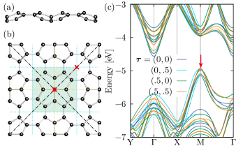
Figure 1: Side view (a) and the top view (b) of the lattice structure of monolayer C₅₆₈. In the top view, a unit cell is also indicated. (c) Band structures of untwisted bilayers with several selected displacements $\bm{\tau}$. In the picture, $\bm{\tau}$ is indicated in the unit of $a_{0}$.

The lattice structure of monolayer C₅₆₈ is shown in Figs. 1(a) and 1. Interestingly, the network consists of mixture of sp³ and sp² bondings, where the four sp³ bonds locate at the center of unit cell in Fig. 1(b). Due to the sp³ nature, the monolayer is buckled as clearly seen in Fig. 1(a). A key monolayer symmetry is roto-inversion $S_{4}$ associated with the sp³ bonds, which can equivalently be expressed as $C_{4z}\mathcal{M}_{xy}$, where $\mathcal{M}_{xy}$ is a reflection with respect to the plane of monolayer. Note that $S_{4}$ automatically gives $C_{2z}$ with respect to the $S_{4}$ center. (Due to the lattice translation symmetry, there appears the other $S_{4}$ center at the corner of a unit cell.) The monolayer breaks inversion symmetry. The other important symmetry is reflection with respect to the plane perpendicular to the layer and running along horizontal or vertical directions in Fig. 1(b). The plane passes through either the center or the corner of a unit cell. There is also a $C_{2}$ axis along the diagonal direction in Fig. 1(b). This in-plane $C_{2}$ operation can be decomposed into $\mathcal{M}_{xy}$ and a reflection with respect to the diagonal lines in Fig. 1(b), which we name $\mathcal{M}_{d}$.

Monolayer C₅₆₈ is predicted has been [8] to be a semiconductor with its valence top at the $M$-point in the Brillouin zone. These crystalline and electronic structures are reproduced in our DFT calculations, see Appendix A for computational details. In this paper, we focus on electronic structures near the valence top.

The moiré pattern in twisted bilayer stems from the position dependence of relative shift $\bm{\tau}$ between two layers. For small twist angles, a moiré system is locally well approximated by untwisted bilayer with relative lateral shift $\bm{\tau}$, and investigating $\bm{\tau}$-dependence of band energy near the valence top in the untwisted bilayer gives information for constructing a moiré twisted bilayer model. Since monolayer C₅₆₈ breaks spatial inversion symmetry, there are two types of stacking patterns: one with two identical copies of monolayers and one between two inversion images of each other. The former still breaks inversion symmetry after stacking while the latter restores inversion symmetry after stacking. In this paper, we focus on the former with the aim of realizing the square lattice Hubbard model in twisted bilayers.

Investigation of $\bm{\tau}$-dependence starts with deriving $\bm{\tau}$-dependence of the layer distance, which corresponds to corrugation in moiré bilayers. For this, we derive total energies within DFT for each $\bm{\tau}$ as functions of interlayer distance with fixed intralayer coordinates, and determine the optimized distance by minimizing the total energy. (See Appendix for details.) Using the optimized distance for each $\bm{\tau}$, the band structures are derived in a normal procedure in DFT. Because of layer doubling, there are two bands near the valence top, and the energies of these two bands are used in extracting parameters for an effective model. Figure 1(c) shows bilayer band structures for several selected $\bm{\tau}$s. Focusing on the valence top at M-point, sizable $\bm{\tau}$ dependence is observed, indicative of strong band reconstruction in twisted bilayer cases.

The effective continuum model for untwisted bilayer expanded near the Brillouin zone corner $\bm{k}_{M}$ can be written as

$$H=H_{0}(\bm{k}_{M})\sigma_{0}+V_{\text{pot}}(\bm{\tau}),\quad V_{\text{pot}}(\bm{\tau})=\sum_{a=0}^{3}V_{a,\bm{k}_{M}}(\bm{\tau})\sigma_{a},$$ (1)

where $V_{\text{pot}}$ describes the the layer potential. $\sigma_{a}$ label the Pauli matrices acting in the layer space and $\sigma_{0}$ is identity. The associated energies are

$$E_{\pm}(\bm{k}_{M},\bm{\tau})=H_{0}(\bm{k}_{M})+V_{0,\bm{k}_{M}}(\bm{\tau})\pm\left(\sum_{a=1}^{3}V_{a,\bm{k}_{M}}(\bm{\tau})^{2}\right)^{1/2}.$$ (2)

We choose the zero-energy level $H_{0}(\bm{k}_{M})=0$ for convenience and will omit the subscript $\bm{k}_{M}$ in $V_{a}$ from now on. The $V$-functions can be determined by comparing these energies with the DFT results.

The symmetry of $V_{\text{pot}}$ is essential for constructing an effective model. In the monolayer case, roto-inversion symmetry $S_{4}=C_{4z}\mathcal{M}_{xy}$. For bilayers, $\mathcal{M}_{xy}$ interchanges two layers, therefore the $S_{4}$ constraint reads

$$V_{\text{pot}}(C_{4z}\bm{\tau})=\sigma_{1}V_{\text{pot}}(\bm{\tau})\sigma_{1}.$$ (3)

More specifically $V_{0,1}(C_{4z}\bm{\tau})=V_{0,1}(\bm{\tau})$ and $V_{2,3}(C_{4z}\bm{\tau})=-V_{2,3}(\bm{\tau}).$ The monolayer in-plane $C_{2}=\mathcal{M}_{d}\mathcal{M}_{xy}$, and leads to

$$V_{\text{pot}}(\mathcal{M}_{d}\bm{\tau})=\sigma_{1}V_{\text{pot}}(\bm{\tau})\sigma_{1}.$$ (4)

Specifically this gives constraints $V_{0,1}(\mathcal{M}_{d}\bm{\tau})=V_{0,1}(\bm{\tau})$ and $V_{2,3}(\mathcal{M}_{d}\bm{\tau})=-V_{2,3}(\bm{\tau}).$ Lastly, since the M-point is a high symmetry point in the Brillouin zone, quantum interference can eliminate interlayer tunneling for specific $\bm{\tau}$ points [34, 5]. In this case, the reflection symmetry in monolayer leads to $V_{1,2}(\bm{\tau})=0$ when $\bm{\tau}$ is at the boundary of a unit cell. In addition, on the diagonal lines in the unit cell which satisfy $\mathcal{M}_{d}\bm{\tau}=\bm{\tau}$, $V_{3}$ vanishes. Also, since M-point is time reversal invariant momentum, there exists a basis such that the Hamiltonian becomes real. In that basis, $V_{2}$ is zero and there remain three functions to be determined.

However, easily obtained inputs from DFT are only two functions, $E_{\pm}(\bm{k}_{M},\bm{\tau})$. To overcome this issue, we adopt lower harmonics expansion of $V_{i}$ respecting crystalline symmetries, and fix required coefficients by the least square fitting to DFT data. (See Appendix B for details.) The prepared lower harmonics expansions are

$$\begin{split}V_{0}(\bm{\tau})=&\ \gamma_{0}+\gamma_{1}(\cos\tilde{\tau}_{x}+\cos\tilde{\tau}_{y})+2\gamma_{2}\cos(\tilde{\tau}_{x})\cos(\tilde{\tau}_{y})\\ &+\gamma_{3}(\cos 2\tilde{\tau}_{x}+\cos 2\tilde{\tau}_{y})\\ &+2\gamma_{4}(\cos(2\tilde{\tau}_{x})\cos(\tilde{\tau}_{y})+\cos(\tilde{\tau}_{x})\cos(2\tilde{\tau}_{y})),\\ V_{1}(\bm{\tau})=&\alpha_{1}\cos\frac{\tilde{\tau}_{x}}{2}\cos\frac{\tilde{\tau}_{y}}{2}\\ &+\alpha_{2}\big{(}\cos\frac{3\tilde{\tau}_{x}}{2}\cos\frac{\tilde{\tau}_{y}}{2}+\cos\frac{\tilde{\tau}_{x}}{2}\cos\frac{3\tilde{\tau}_{y}}{2}\big{)},\\ V_{3}(\bm{\tau})=&\beta_{1}(\cos\tilde{\tau}_{x}-\cos\tilde{\tau}_{y})+\beta_{2}(\cos 2\tilde{\tau}_{x}-\cos 2\tilde{\tau}_{y})\\ &+\beta_{3}(\cos 3\tilde{\tau}_{x}-\cos 3\tilde{\tau}_{y}),\end{split}$$ (5)

where $\tilde{\tau}_{\mu}=2\pi\tau_{\mu}/a_{0}$. These expansions satisfy all the symmetry constraints described above.

When fitting with the DFT data, coefficients in $V_{0}$ can be determined using a data set $(E_{+}+E_{-})/2$. The remaining data set $(E_{+}-E_{-})/2$ can be used for determining two functions $V_{1}$ and $V_{3}$: at the boundary of a unit cell, $V_{1}=0$ and $(E_{+}-E_{-})/2$ is solely determined from $V_{3}$; on the other hand, on the diagonal lines in a unit cell that satisfies $\mathcal{M}_{d}\bm{\tau}=\bm{\tau}$, the symmetry constraints leads to $V_{3}=0$, and $(E_{+}-E_{-})/2$ is solely determined from $V_{1}$. Using these facts, we obtain

$$\begin{split}&\alpha_{1}=0.194,\ \alpha_{2}=-0.052,\ \gamma_{0}=-2.292,\\ &\gamma_{1}=-0.011,\ \gamma_{2}=0.021,\ \gamma_{3}=-0.007,\ \gamma_{4}=-0.001,\\ &\beta_{1}=-0.024,\ \beta_{2}=-0.008,\ \beta_{3}=-0.011,\end{split}$$ (6)

all in the unit of eV. The lower harmonics expansion and the DFT results are compared in Fig. 2. Considering the simplicity of the approximation and limitation in converting $E_{\pm}$ data set to the coefficients, the match between the data and the lower harmonics expansion is remarkable.

Figure 2: $E_{+}(\bm{k}_{M},\bm{\tau})$ and $E_{-}(\bm{k}_{M},\bm{\tau})$ obtained with the lower harmonics expansion (lines) and DFT (points).

III Twisted bilayer model

In this section, we specify to the rigid twist case with dispacement $\bm{\tau}(\bm{r})=2\sin\frac{\theta}{2}\hat{z}\times\bm{r}.$ The moiré lattice constant is thus $a_{M}\approx a_{0}/\theta$ at small twisting angles. We will denote the moiré lattice vectors by $\bm{R}_{1},\bm{R}_{2}$ and the moiré reciprocal lattice vectors by $\bm{q}_{1},\bm{q}_{2}$. The continuum Hamiltonian reads

$$H=\begin{pmatrix}H_{-}(-i\bm{\nabla})+V_{0}+V_{3}&e^{\mathrm{i}\bm{\delta k}\cdot\bm{r}}V_{1}\\ e^{-\mathrm{i}\bm{\delta k}\cdot\bm{r}}V_{1}&H_{+}(-i\bm{\nabla})+V_{0}-V_{3}\end{pmatrix},$$ (7)

where $H_{\pm}(-i\bm{\nabla})=\frac{\hbar^{2}}{2m_{*}}(-i\bm{\nabla}-\bm{k}_{M}\pm\delta\bm{k}/2)^{2}$ and $\delta\bm{k}=2\sin\frac{\theta}{2}(\hat{\bm{z}}\times\bm{k}_{M})=(\bm{q}_{1}-\bm{q}_{2})/2,$ which is depicted in Fig. 3.

When $V_{0}=V_{3}=0$ and in (7) and keeping only the leading term in $V_{1}$, i.e., $V_{1}=\alpha_{1}\cos(\frac{\pi}{a_{0}}\tau_{1})\cos(\frac{\pi}{a_{0}}\tau_{2})=\alpha_{2}\cos(\frac{\pi}{a_{M}}y)\cos(\frac{\pi}{a_{M}}x),$ the model reduces to that studied in [6]: there is an emergent symmetry at small twisting angles $\mathcal{L}_{0}=\sigma_{x}e^{i\sigma_{z}\delta\bm{k}\cdot\bm{r}}$. This symmetry forces the band maxima to be degenerate $E_{\Gamma}=E_{M}$ leads to the vanishing of nearest neighbor hopping in the effective tight binding model defined on the moiré lattice. Adding $V_{0}$ as well as the sub-leading terms in $V_{1}$ don’t change the physics.

A finite $V_{3}$ term breaks $\mathcal{L}_{0}$, but a variation of it which involves the fourfold rotation remains as an approximate symmetry at small twisting angles. To understand the effect of the emergent symmetry on the moiré momentum space, we apply the following convenient unitary transformation ${\mathcal{U}}=e^{i\bm{k}_{0}\cdot\bm{r}}\sigma_{0}$ where $\bm{k}_{0}=\bm{k}_{M}+(\bm{q}_{1}+\bm{q}_{2})/4$ , such that ${H}^{\prime}={\mathcal{U}^{\dagger}}H{\mathcal{U}}$ has similar form as in (7) but with $H_{\pm}$ replaced by $H_{\pm}^{\prime}=\frac{\hbar^{2}}{2m_{*}}(-i\bm{\nabla}-\bm{k}_{\bm{M}}+\bm{k}_{0}\pm\delta\bm{k}/2)$. We can now label any momentum using its shift from $\bm{k}_{0}:$ $\bm{q}=\bm{k}-\bm{k}_{0}$, where $\bm{k}_{0}$ is the $\Gamma_{m}$ point in the shifted Brillouin zone plotted in the right panel of figure 3. Then we conveniently have

$$\begin{split}&H_{+}^{\prime}=\frac{\hbar^{2}}{2m_{*}}(-i\bm{\nabla}+\bm{q}+\bm{q}_{1}/2)^{2},\\ &H_{-}^{\prime}=\frac{\hbar^{2}}{2m_{*}}(-i\bm{\nabla}+\bm{q}+\bm{q}_{2}/2)^{2}.\end{split}$$ (8)

It is easy to check (details are shown in appendix D) that the following operation leaves the Hamiltonian invariant:

$$\mathcal{L}=e^{-\frac{\mathrm{i}}{2}\bm{q}_{2}\cdot\bm{r}(\sigma_{3}+\sigma_{0})/2}\sigma_{1}C_{4z},\quad H^{\prime}(\bm{q})=\mathcal{L}H^{\prime}(R_{\pi/2}\bm{q})\mathcal{L}^{-1}.$$ (9)

Figure 3: Left: Brillouin zones of the top and bottom layers. Dashed blue square is the moiré Brillouin zone, and dashed red square is the shifted moiré Brillouin zone under the transformation $U$. Right: High symmetry points in the shifted moiré Brillouin zone. $\Gamma_{m}$ point has momentum $\bm{k}_{0}.$

Consequently, as long as the band is non-degenerate, the energy of the Hamiltonian $H^{\prime}$ must satisfy

$$E(\bm{q})=E(R_{\pi/2}\bm{q}),$$ (10)

which leads to $E(X_{m})=E(Y_{m})$ in the shifted moiré Brillouin zone shown in fig. 3.

Using the fitted parameters found in (6) and keeping only those whose magnitudes are larger than $0.01$ eV , we show the band structure $E(\bm{q})$ along high symmetry lines in fig. LABEL:fig:band: the band top lives at the $M_{m}$ point, and the band bottom is at the $\Gamma_{m}$ point in the shifted Brillouin zone. The shoulders at $X_{m}$ and $Y_{m}$ points have the same energies consistent with (10). The band structure LABEL:fig:band clearly resembles that of the tight-binding Hamiltonian on square lattice with nearest neighbor hopping.

For example at $\theta=1.8^{\circ}$, the flat moiré band is separated from the neighboring band by a large gap of $\sim 4.2$ meV, which is about $300$ times the bandwidth of the top flat band.

III.1 Displacement field

Upon adding a displacement field $D\sigma_{z},$ the emergent $\mathcal{L}$ symmetry which involves layer exchange is absent. In the shifted moiré Brillouin zone plotted in the right panel of fig. 3, this translates into the asymmetry $E_{X}\neq E_{Y}.$ Taking into account all the terms in the Hamiltonian, a small and negative $D$ already shifts the band extrema: $E_{Y}>E_{M}>E_{\Gamma}>E_{X}$. Further increasing the magnitude, when $D=-0.17$ eV, band crossings between the top two moiré bands are induced, and beyond which $E_{M}<E_{\Gamma}$. The band crossings always happen along the Brillouin zone boundary which respects the reflection symmetry. See Fig. LABEL:fig:D for typical band structures. For the a positive $D$, the evolution of band structures is similar but with $X\leftrightarrow Y$ exchanged.

IV Tight binding model

In this section we analyze the effective tight-binding model for the twisted bilayer. At small twisting angles, it is sufficient to include only the nearest neighbor $t_{x},t_{y}$ and the next nearest neighbor hoppings $t_{x+y}$, $t_{x-y}$. Time reversal symmetry requires them to be real. Reflection symmetries with respect to the $x$- and $y$- axes require the next nearest neighbor hoppings, $t_{x+y}=t_{x-y}$. The corresponding dispersion is:

$$E(\bm{k})=E_{0}-t_{x}\cos k_{x}-t_{y}\cos k_{y}-2t_{x+y}\cos k_{x}\cos k_{y}.$$ (11)

The emergent $\mathcal{L}$ symmetry, when present, imposes that the nearest neighbor hopping $t_{x}=t_{y}$.

IV.1 The hopping parameters

The four parameters $\{E_{0},t_{x},t_{y},t_{x+y}\}$ can be easily solved by requiring that at high symmetry points $\Gamma_{m},X_{m},Y_{m},M_{m}$ defined in fig. 3, the energies computed from the twisted bilayer model and that from the tight binding model (11) should match with each other. This method works well at small twisting angles where the longer ranged hoppings can be ignored. For example at $D=0$ and $\theta=3.6^{\circ}$, we have $t_{x}=t_{y}=0.171$ meV, $t_{1}=0.014$ meV. We plot the dispersions calculated both from the tight-binding model and the lowest-harmonics twisted bilayer model in fig. 6 below and they match nicely.

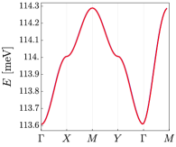
Figure 6: Top bands structures at $D=0,\theta=3.6^{\circ}.$ Calculation from the twisted bilayer model is shown in blue, and that from the tight-binding model is shown in red - they completely overlap.

While one can also plot $t$ as a function of twisting angle and displacement field using this simple method, below we will perform a more careful numerical examination.

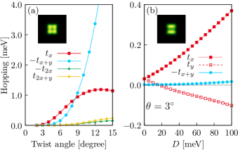
Figure 7: Hopping parameters derived using full parameters and Wannier functions. (a) Twist angle dependence. $t_{1}$ to $t_{4}$ correspond to the first to the fourth nearest neighbor hoppings in the square lattice. (b) Displacement field dependence for $\phi=3^{\circ}$. Insets: total charge (sum of the charges on the upper and the lower layer) for a Wannier function at $\phi=3^{\circ}$ with (a) $D=0$ and (b) $D=50$ meV.

The elaboration is done in the following aspects: (i) taking all $\gamma_{i}$, $\alpha_{i}$, and $\beta_{i}$ into account, and (ii) deriving the Wannier orbitals for the highest energy band. In the parameter range showing no crossing between the top and second bands, the highest energy band is well isolated from the other bands, and it is justified to have reasonably localized Wannier orbitals. In practice, we prepare Bloch wave functions for the highest energy band in the continuum Hamiltonian Eq. (7) (with full account of $\gamma_{i}$, $\alpha_{i}$, and $\beta_{i}$) on $13\times 13$ regular grid in the moire Brillouin zone, and project them to an ansatz Gaussian function to fix the phases required in constructing Wannier functions. (This procedure is the same as the projection on initial guess functions in Ref. [35].)

The obtained hopping parameters are plotted in Fig. 7. The angle dependence without displacement field is summarized in Fig. 7(a). A characteristic crossover from the regime $|t_{x}|<|t_{x+y}|$ to the regime $|t_{x}|>|t_{x+y}|$ takes place at around $8.5^{\circ}$ as the twist angle is decreased. Within the investigated range of the twist angle, $|t_{2x}|$ and $|t_{2x+y}|$ are significantly smaller than $|t_{x}|$ and $|t_{x+y}|$, indicating the validity of the model Eq. (11). The displacement field $D$ dependence at $\theta=3^{\circ}$ is shown in Fig. 7(b). As we have seen in the simplified model, $t_{x}=t_{y}$ for $D=0$ due to the emergent $\mathcal{L}$ symmetry, and finite $D$ lifts this degeneracy. Interestingly, there is a point where $t_{y}=0$, i.e., almost purely one-dimensional state. (There remains slight two-dimensional nature due to small but finite $|t_{x+y}|$ and longer range hoppings.) In the large $D$ side, $|t_{x}|$ and $|t_{y}|$ grows much faster than $|t_{x+y}|$.

The insets in Fig. 7 show the typical Wannier functions where the color corresponds to the sum of the wave function weights for the upper and the lower layers, which we write $\rho(\bm{r})$. The $S_{4}$ symmetry involves the layer exchange, but if we focus on the sum over the two layers, $\rho(\bm{r})$ should look $C_{4}$ symmetric for $D=0$, which is consistent with the inset of Fig. 7(a). On the other hand, finite $D$ breaks the $S_{4}$ symmetry, $\rho(\bm{r})$ should look distorted, which is consistent with the inset of Fig. 7(b).

IV.2 Hubbard $U$ parameters

Having the Wannier functions, the matrix elements for Coulomb interaction, in other words the Hubbard $U_{\bm{R}}$ parameters can be estimated, where $\bm{R}$ represents relative coordinate between two Wannier functions. We have adapted the formula

$$\begin{split}U_{\bm{R}}&=\int d^{2}\bm{r}\rho(\bm{r}+\bm{R})V(\bm{r}-\bm{r}^{\prime})\rho(\bm{r}^{\prime})\\ &=\int\frac{d^{2}\bm{q}}{(2\pi)^{2}}\rho_{\bm{q}}\rho_{-\bm{q}}V_{\bm{q}}e^{-i\bm{q}\cdot\bm{R}},\end{split}$$ (12)

where $\rho_{\bm{q}}$ is a Fourier component of $\rho(\bm{r})$, and

$$V_{\bm{q}}=\frac{e^{2}}{2\epsilon\epsilon_{0}|\bm{q}|}\tanh(|\bm{q}|\xi).$$ (13)

Here, we assume that the Coulomb interaction is screened by top and bottom metallic gates placed with the distance $\xi$ from the sample [36, 37, 38]. From Eq. (13), we can see that the screening effect is significant when the length scale $1/|\bm{q}|$ is much larger than $\xi$. Note that this is an estimation of the upper limit of $U$ because the screening effect from higher energy bands in addition to the one from the substrate has been ignored.

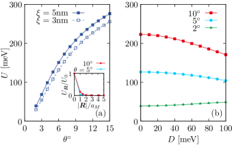
Figure 8: Hubbard $U$ estimated using the Wannier functions. (a) Twist angle dependence for $\xi=3$nm and $\xi=5$nm. Inset shows $|\bm{R}|$ dependence at $\xi=3$nm. (b) Displacement field dependence for selected twisted angles with $\xi=5$nm.

The twist angle dependence of $U\equiv U_{0}$ without displacement field is plotted in Fig. 8(a). Here, we employ $\epsilon=6$, a typical value for a hBN substrate, to take into account the screening effect from the substrate. The Hubbard $U$ is typically in the range of a few hundreds of meV, which is significantly larger than the hopping parameters. As the twist angle gets smaller, $U$ is also decreasing since the moiré length scale becomes larger. Figure 8(b) is for the displacement field dependence, showing that $U$ only weakly or moderately depends on $D$. The inset of Fig. 8(a) is for $|\bm{R}|$ dependence of $U_{\bm{R}}$ with $\xi=3$nm, showing rapid decay of $U_{\bm{R}}$. The decay rate is determined by the screening effect from the metallic gates, and depends on the twist angle, since the length scale is different for different twist angles.

In order to have an intuition on the size of $U$, we estimate the Coulomb interaction via $U(\epsilon)=\frac{e^{2}}{4\pi\epsilon\epsilon_{0}l}$, where $l$ is the size of the Wannier orbital. The latter can be obtained from the harmonic oscillator approximation of the leading moiré potential $\alpha_{1}:$

$$\frac{\hbar^{2}}{2m_{*}}\frac{1}{l^{2}}=\frac{1}{2}\alpha_{1}\pi^{2}\frac{l^{2}}{a_{M}^{2}}.$$ (14)

Inserting realistic numbers $m_{*}=0.64m_{0},$ $a_{0}=5.725$Å, we can solve $l=1.6515$ nm at $\theta=3^{\circ}$ and $D=0$. If the relative permittivity is taken to be $\epsilon=6,$ it leads to $U=0.1453$ eV, which is significantly larger than the bandwidth of $0.2984$ meV for the same parameter choice. If instead one plugs in the $l$ found from Wannier function calculations described above, at $\theta=3^{\circ}$ we would have $l=2.9562$ nm and $U=0.0812$ eV. These estimates match with the orders of magnitude in first-principle calculation, but the detailed discrepancies could be due to the oversimplified treatment where we only take into account $\alpha_{1}$ and the spherical approximation of the potential.

V Discussion

We proposed twisted homobilayer C₅₆₈ to be a promising device in realizing the (extended) single-band square-lattice Hubbard model. If successfully fabricated, the device could shed important light on the mechanism of high temperature superconductivity realized in other square lattice materials. At negligible displacement field, the system is naturally in the strong coupling limit, exhibiting a remarkably high $U/t$ ratio. For instance, when the twisting angle is at $3^{\circ}$ and $9^{\circ}$, the $U/t$ ratio is of the order $10^{5}$ and $10^{2}$, respectively. One can then probe the intermediate temperature regime, of $t\ll T\ll U$, which is hard to achieve in electronic materials. Taking into account additional screening effects from higher energy bands, we expect these $U/t$ values to decrease, potentially reaching a minimum value of $U/t\sim 10$, a regime closely resembling cuprate physics. Additionally, the bilayer offers great flexibility: by tuning the twisting angle, a wide range of ratios between next-nearest-neighbor and nearest-neighbor hoppings can be achieved. Furthermore, the introduction of a displacement field induces anisotropy between hoppings in different directions $t_{x},t_{y}$. The orientation of this anisotropy can be rotated by $90^{\circ}$ simply by reversing the sign of the vertical electric field. Notably, within an experimentally accessible range, the hopping amplitudes can change sign upon increasing $|D|$, with $t_{y}$ $(t_{x})$ crossing from positive to negative when $D>0$ $(D<0)$.

In addition to reproducing the target single-band square lattice Hubbard model, twisted homobilayer C₅₆₈ can host interesting new phenomena. One possibility is tunable metal-insulator transition. Fig. 9 plots the bandwidth of the top moiré band. Away from band crossing, the bandwidth reflects the magnitudes of the hopping amplitudes in the system. Comparing with the onsite Coulomb energy shown in Fig. 8, we see that at larger twisting angles and larger displacement fields (such that the system is highly anisotropic), the Coulomb interaction can have the same order of magnitude as that of the bandwidth. Consequently, there can potentially be a metal-insulator transition tuned by displacement field. However, we have also shown in Fig. LABEL:fig:D that the top two moiré bands will cross at larger displacement fields $|D|\sim 170$ meV. Therefore, a full description of the potential transition requires a two-band tight-binding model. Since the large parameter space is beyond the scope of the current paper, we leave a careful examination for future work.

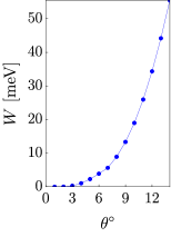
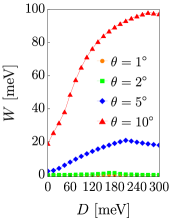
Figure 9: Left: Band width $W$ as a function of twisting angle when displacement field $D=0$. Right: Band width as a function of $D$ for different twisting angles.

Another interesting variation of the model is the following. In this paper, we focus on the stacking of two identical copies of a monolayer. In the case of the other type of stacking, i.e., stacking between inversion images, both of Eqs. (3) and (4) reduce to

$$V_{\text{pot}}(\bm{\tau})=\sigma_{1}V_{\text{pot}}(\bm{\tau})\sigma_{1},$$ (15)

which kills $V_{2,3}$ and induces no constraint on $V_{0,1}$. When there is no constraint, there is no reason for low energy effective model to have the symmetry of the square lattice. Namely, we expect $|t_{x}|\neq|t_{y}|$ even in the absence of a displacement fields. Thus, the successful fabrication of this family of structures would both shed important light on old problems and stimulate a host of new investigations.

Appendix A Density functional theory

In this study, the density functional theory calculations have been done using Quantum Espresso package [39, 40]. For the exchange-correlation functional, we have adopted rev-vdW-DF2 functional [41] to take van der Waals forces into account. Pseudopotentials are from PSlibrary [42, 43], and we use projector augmented wave method to include core state information in pseudopotentials. In order to handle our target two-dimensional material, a 30Å thick supercell in $z$-direction is used. The parameters for our continuum model are derived with a naive supercell method, but we have confirmed that dipole field effects are small and our conclusions are not affected.

Appendix B Lower harmonics expansion and the least square fit

Let us assume $\bm{\tau}$ dependence of some physical quantity $Q(\bm{\tau})$ can be written as

$$Q(\bm{\tau})=\sum_{l=1}^{N}c_{l}g_{l}(\bm{\tau})$$ (16)

where each $g_{l}(\bm{\tau})$ function is some combination of harmonic functions that respects symmetry and periodicity of the system. Here, $N$ is the number of coefficients, or in other words, the number of degrees of freedom. On the other hand, let us assume that we have data (from DFT) for that quantity $D(\bm{\tau})$ on some finite grid in $\bm{\tau}$ space. Basically, $c_{l}$ is simply fixed by minimizing

$$\Xi=\sum_{\bm{\tau}\in\text{grid}}|Q(\bm{\tau})-D(\bm{\tau})|^{2}.$$ (17)

However, we sometimes want to apply constraints. For instance, we may take a special care about the values at $\bm{\tau}$ with high symmetry, e.g., $\bm{\tau}$ at zone corners or zone boundaries. Then, $\Xi$ is minimized under the condition that $Q(\bm{\tau})$ values at selected $\bm{\tau}$ points are pinned down to $D(\bm{\tau})$. Let $N_{c}$ be the number of constraints. Then, $N_{c}$ should not exceed $N$. For convenience, $N_{c}$ constrained grids are labeled by $i$. We first define $N_{c}\times N_{c}$-matrix $\hat{A}$, $N_{c}\times(N-N_{c})$-matrix $\hat{B}$, and $N_{c}$-dimensional vector $\bm{D}$ as

$$A_{i,l} =g_{l}(\bm{\tau}_{i}),\quad(l\leq N_{c})$$ (18)

$$B_{i,l-N_{c}} =g_{l}(\bm{\tau}_{i}),\quad(l>N_{c})$$ (19)

$$D_{i} =D(\bm{\tau}_{i}).$$ (20)

Using these entities, $N_{c}$-dimensional vector $\bm{C}^{(0)}$ and $(N-N_{c})\times N_{c}$-matrix $\bm{C}^{(1)}$ are defined as

$$\bm{C}^{(0)} =\hat{A}^{-1}\bm{D},$$ (21)

$$\hat{C}^{(1)} ={}^{t}(\hat{A}^{-1}\hat{B}).$$ (22)

Now, new functions $\tilde{g}_{l}(\bm{\tau})$ for $l>N_{c}$ are introduced as

$$\tilde{g}_{l}(\bm{\tau})=g_{l}(\bm{\tau})-\sum_{l^{\prime}=1}^{N_{c}}C^{(1)}_{l-N_{c},l^{\prime}}g_{l^{\prime}}(\bm{\tau}),$$ (23)

and the constrained function $Q(\bm{\tau})$ is written as

$$Q(\bm{\tau})=\sum_{l=1}^{N_{c}}C^{(0)}_{l}g_{l}(\bm{\tau})+\sum_{l>N_{c}}^{N}c_{l}\tilde{g}_{l}(\bm{\tau}).$$ (24)

Note that we have $\tilde{g}_{l}(\bm{\tau}_{i})=0$, which is confirmed as

$$\begin{split}\tilde{g}_{l}(\bm{\tau}_{i})&=B_{i,l-N_{c}}-\sum_{l^{\prime}=1}^{N_{c}}(\hat{A}^{-1}\hat{B})_{l^{\prime},l-N_{c}}A_{i,l^{\prime}}\\ &=B_{i,l-N_{c}}-(\hat{A}\hat{A}^{-1}\hat{B})_{i,l-N_{c}}=0,\end{split}$$ (25)

and we have $Q(\bm{\tau}_{i})=D(\bm{\tau}_{i})$, which is confirmed as

$$\begin{split}Q(\bm{\tau}_{i})&=\sum_{l=1}^{N_{c}}(\hat{A}^{-1}\bm{D})_{l}A_{i,l}\\ &=(\hat{A}\hat{A}^{-1}\bm{D})_{i}=D(\bm{\tau}_{i}).\end{split}$$ (26)

To minimize $\Xi$, we take derivative of $\Xi$ with respect to $c_{l}$, leading to

$$\frac{\partial\Xi}{\partial c_{l}}=2\sum_{l^{\prime}}M_{l,l^{\prime}}c_{l^{\prime}}-2X_{l},$$ (27)

where

$$M_{l,l^{\prime}} =\sum_{\bm{\tau}\in\text{grid}}\tilde{g}_{l}(\bm{\tau})\tilde{g}_{l^{\prime}}(\bm{\tau}),$$ (28)

$$X_{l} =\sum_{\bm{\tau}\in\text{grid}}\tilde{g}_{l}(\bm{\tau})(D(\bm{\tau})-\sum_{l^{\prime}}C^{(0)}_{l^{\prime}}g_{l^{\prime}}(\bm{\tau})).$$ (29)

Then, the optimized $c_{l}$ can be obtained from

$$\bm{c}=\hat{M}^{-1}\bm{X}.$$ (30)

Appendix C Interlayer distance

To obtain $E_{\pm}(\bm{k}_{M},\bm{\tau})$ within DFT, we need to estimate the interlayer distance $d_{z}$ for each $\bm{\tau}$. We first derive $d_{z}$ dependence of the total energy within DFT, and choose $d_{z}$ that realizes minimum total energy. While scanning over $d_{z}$, the intralayer coordinates are fixed. Note that if in-plane relaxation is also allowed, $\bm{\tau}$ can flow into the one with lower total energy, which prevents us from getting $\bm{\tau}$ dependence. In practice, $d_{z}$-scan is done over finite set of $d_{z}$ values. Then, for each $\bm{\tau}$, the obtained data are used to fit an approximated expression

$$E_{\text{tot}}(d_{z})=\alpha e^{-\beta(d_{z}-d_{0})}-\gamma\Bigl{(}\frac{d_{0}}{d_{z}}\Bigr{)}^{\delta}.$$ (31)

Here, $d_{0}$ is chosen to be 4Å, and $\{\alpha,\beta,\gamma,\delta\}$ are the adjustable parameters in the fitting. The fitting is done with FindFit function in Mathematica.

The $\bm{\tau}$ dependence is approximated by

$$\begin{split}d_{z}(\bm{\tau})=c_{0}&+c_{1}(\cos\tilde{\tau}_{x}+\cos\tilde{\tau}_{y})\\ &+c_{2}(\cos(\tilde{\tau}_{x}+\tilde{\tau}_{y})-\cos(\tilde{\tau}_{x}+\tilde{\tau}_{y}))\\ &+c_{3}(\cos 2\tilde{\tau}_{x}+\cos 2\tilde{\tau}_{y})\\ &+c_{4}(\cos(2\tilde{\tau}_{x}+\tilde{\tau}_{y})+\cos(\tilde{\tau}_{x}+2\tilde{\tau}_{y})\\ &\quad\quad+\cos(2\tilde{\tau}_{x}-\tilde{\tau}_{y})+\cos(\tilde{\tau}_{x}-2\tilde{\tau}_{y})).\end{split}$$ (32)

The coefficients are fixed by the constrained least square algorithm above. Here, DFT calculations are done on $8\times 8$ regular grids in a unit cell, and the constraint is such that the fitting faithfully reproduce the DFT results at $\bm{\tau}=(0,0)$, $(a_{0}/2,0)$, and $(a_{0}/2,a_{0}/2)$, which correspond to the unit cell center, the center of the unit cell edge, and the unit cell corner, respectively. Using the obtained coefficients,

$$c_{0}=3.896,\,c_{1}=-0.093,\,c_{2}=0.007$$ (33)

$$c_{3}=0.021,\,c_{4}=-0.028,$$ (34)

which are in the unit of Å, the fitting and the DFT results compare as in Fig. 10, showing satisfactory match between them.

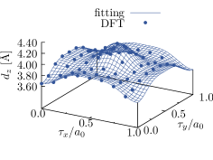
Figure 10: Interlayer distance obtained by the lower harmonics expansion (lines) and DFT (points).

Appendix D Emergent symmetry $\mathcal{L}$

In the convenient basis described near equation (8), the Hamiltonian is

$$H^{\prime}(\bm{q})=\begin{pmatrix}H_{-}^{\prime}(\bm{q})+V_{0}+V_{3}&e^{\mathrm{i}\delta\bm{k}\cdot\bm{r}}V_{1}(\bm{r})\\ e^{-\mathrm{i}\delta\bm{k}\cdot\bm{r}}V_{1}(\bm{r})&H_{+}^{\prime}(\bm{q})+V_{0}-V_{3}\end{pmatrix}.$$ (35)

Under $C_{4z}$ rotation, different terms in the Hamiltonian transforms as

$$\begin{split}&C_{4z}H^{\prime}_{+}(\bm{q})C_{4z}^{-1}\\ =&\frac{\hbar^{2}}{2m_{*}}\left[-i\bm{\nabla}+R_{-\pi/2}\bm{q}+R_{-\pi/2}\bm{q}_{1}/2\right]^{2}\\ =&\frac{\hbar^{2}}{2m_{*}}\left[-i\bm{\nabla}+R_{-\pi/2}\bm{q}-\bm{q}_{2}/2\right]^{2}\\ =&e^{\mathrm{i}\bm{q}_{2}\cdot\bm{r}}H_{-}^{\prime}(R_{-\pi/2}\bm{q})e^{-\mathrm{i}\bm{q}_{2}\cdot\bm{r}}.\end{split}$$ (36)

Similarly,

$$\begin{split}&C_{4z}H^{\prime}_{-}(\bm{q})C_{4z}^{-1}\\ =&\frac{\hbar^{2}}{2m_{*}}\left[-i\bm{\nabla}+R_{-\pi/2}\bm{q}+R_{-\pi/2}\bm{q}_{2}/2\right]^{2}\\ =&\frac{\hbar^{2}}{2m_{*}}\left[-i\bm{\nabla}+R_{-\pi/2}\bm{q}+\bm{q}_{1}/2\right]^{2}=H^{\prime}_{+}(R_{-\pi/2}\bm{q}).\end{split}$$ (37)

As for the moiré potentials,

$$V_{0,1}(R_{\pi/2}\bm{r})=V_{0,1}(\bm{r}),\quad V_{3}(R_{\pi/2}\bm{r})=-V_{3}(\bm{r}).$$ (38)

Putting everything together, the whole Hamiltonian transforms as

$$\begin{split}&C_{4z}\tilde{H}(\bm{q})C_{4z}^{-1}=V_{0}\sigma_{0}-V_{3}\sigma_{3}\\ &\quad\quad+\begin{pmatrix}H_{+}^{\prime}(R_{-\pi/2}\bm{q})&e^{\mathrm{i}\delta\bm{k}\cdot R_{\pi/2}\bm{r}}V_{1}\\ e^{-\mathrm{i}\delta\bm{k}\cdot R_{\pi/2}\bm{r}}V_{1}&e^{\mathrm{i}\bm{q}_{2}\cdot\bm{r}}H_{-}^{\prime}(R_{-\pi/2}\bm{q})e^{-\mathrm{i}\bm{q}_{2}\cdot\bm{r}})\end{pmatrix}\end{split}$$ (39)

The second line can be further simplified to

$$\begin{split}&\begin{pmatrix}H_{+}^{\prime}(R_{-\pi/2}\bm{q})&e^{\mathrm{i}R_{-\pi/2}\delta\bm{k}\cdot\bm{r}}V_{1}\\ e^{-\mathrm{i}R_{-\pi/2}\delta\bm{k}\cdot\bm{r}}V_{1}&e^{\mathrm{i}\bm{q}_{2}\cdot\bm{r}}H_{-}^{\prime}(R_{-\pi/2}\bm{q})e^{-\mathrm{i}\bm{q}_{2}\cdot\bm{r}})\end{pmatrix}\\ =&\begin{pmatrix}H_{+}^{\prime}(R_{-\pi/2}\bm{q})&e^{-\mathrm{i}\delta\bm{k}\cdot\bm{r}}e^{-\mathrm{i}\bm{q}_{2}\cdot\bm{r}}V_{1}\\ e^{+\mathrm{i}\delta\bm{k}\cdot\bm{r}}e^{\mathrm{i}\bm{q}_{2}\cdot\bm{r}}V_{1}&e^{\mathrm{i}\bm{q}_{2}\cdot\bm{r}}H_{-}^{\prime}(R_{-\pi/2}\bm{q})e^{-\mathrm{i}\bm{q}_{2}\cdot\bm{r}})\end{pmatrix}\end{split}$$ (40)

where we have used

$$R_{-\pi/2}\delta\bm{k}=(-\bm{q}_{1}-\bm{q}_{2})/2=-\delta\bm{k}-\bm{q}_{2}.$$ (41)

Further, applying $e^{-\frac{\mathrm{i}}{2}\bm{q}_{2}\cdot\bm{r}(\sigma_{3}+\sigma_{0})}\sigma_{1}$, we obtain

$$\begin{split}\mathcal{L}\tilde{H}(\bm{q})\mathcal{L}^{-1}=&e^{-\frac{\mathrm{i}}{2}\bm{q}_{2}\cdot\bm{r}(\sigma_{3}+\sigma_{0})}\sigma_{1}C_{4z}\tilde{H}(\bm{q})C_{4z}^{-1}\sigma_{1}e^{\frac{\mathrm{i}}{2}\bm{q}_{2}\cdot\bm{r}(\sigma_{3}+\sigma_{0})}\\ =&\tilde{H}(R_{-\pi/2}\bm{q}).\end{split}$$ (42)

References

- Keimer et al. [2015] B. Keimer, S. A. Kivelson, M. R. Norman, S. Uchida, and J. Zaanen, Nature 518, 179 (2015).
- Kennes et al. [2021] D. M. Kennes, M. Claassen, L. Xian, A. Georges, A. J. Millis, J. Hone, C. R. Dean, D. Basov, A. N. Pasupathy, and A. Rubio, Nature Physics 17, 155 (2021).
- Wu et al. [2018] F. Wu, T. Lovorn, E. Tutuc, and A. H. MacDonald, Phys. Rev. Lett. 121, 026402 (2018).
- Tang et al. [2020] Y. Tang, L. Li, T. Li, Y. Xu, S. Liu, K. Barmak, K. Watanabe, T. Taniguchi, A. H. MacDonald, J. Shan, et al., Nature 579, 353 (2020).
- Kariyado and Vishwanath [2019] T. Kariyado and A. Vishwanath, Phys. Rev. Research 1, 033076 (2019).
- Eugenio et al. [2024] P. M. Eugenio, Z.-X. Luo, A. Vishwanath, and P. A. Volkov, Tunable hubbard models in twisted square homobilayers (2024), arXiv:2406.02448 [cond-mat.str-el] .
- Mounet et al. [2018] N. Mounet, M. Gibertini, P. Schwaller, D. Campi, A. Merkys, A. Marrazzo, T. Sohier, I. E. Castelli, A. Cepellotti, G. Pizzi, et al., Nature nanotechnology 13, 246 (2018).
- Ram and Mizuseki [2020] B. Ram and H. Mizuseki, Carbon 158, 827 (2020).
- Gao” et al. [2020] Q. Gao”, H. Sahin”, and J. Kang”, Strain tunable band structure of a new 2d carbon allotrope c¡sub¿568¡/sub¿ (2020).
- Lu et al. [2022] K. Lu, T. Wang, X. Li, L. Dai, J. Yin, and Y. Ding, Fullerenes, Nanotubes and Carbon Nanostructures 30, 385 (2022), https://doi.org/10.1080/1536383X.2021.1944119 .
- Zhao et al. [2023a] W.-H. Zhao, F.-Y. Li, H.-X. Zhang, R. I. Eglitis, J. Wang, and R. Jia, Applied Surface Science 607, 154895 (2023a).
- Jiang and Devereaux [2019] H.-C. Jiang and T. P. Devereaux, Science 365, 1424 (2019), https://www.science.org/doi/pdf/10.1126/science.aal5304 .
- Chung et al. [2020] C.-M. Chung, M. Qin, S. Zhang, U. Schollwöck, and S. R. White (The Simons Collaboration on the Many-Electron Problem), Phys. Rev. B 102, 041106 (2020).
- Jiang et al. [2020] Y.-F. Jiang, J. Zaanen, T. P. Devereaux, and H.-C. Jiang, Phys. Rev. Res. 2, 033073 (2020).
- Danilov et al. [2022] M. Danilov, E. G. van Loon, S. Brener, S. Iskakov, M. I. Katsnelson, and A. I. Lichtenstein, npj Quantum Materials 7, 50 (2022).
- Lu et al. [2024] X. Lu, F. Chen, W. Zhu, D. N. Sheng, and S.-S. Gong, Phys. Rev. Lett. 132, 066002 (2024).
- Jiang et al. [2021] S. Jiang, D. J. Scalapino, and S. R. White, Proceedings of the National Academy of Sciences 118, e2109978118 (2021), https://www.pnas.org/doi/pdf/10.1073/pnas.2109978118 .
- Jiang et al. [2012] H.-C. Jiang, H. Yao, and L. Balents, Phys. Rev. B 86, 024424 (2012).
- Nomura and Imada [2021] Y. Nomura and M. Imada, Phys. Rev. X 11, 031034 (2021).
- Qian and Qin [2024] X. Qian and M. Qin, Phys. Rev. B 109, L161103 (2024).
- Rückriegel et al. [2024] A. Rückriegel, D. Tarasevych, and P. Kopietz, Phys. Rev. B 109, 184410 (2024).
- Kariyado [2023] T. Kariyado, Phys. Rev. B 107, 085127 (2023).
- Volkov et al. [2023a] P. A. Volkov, J. H. Wilson, K. P. Lucht, and J. H. Pixley, Phys. Rev. B 107, 174506 (2023a).
- Soeda et al. [2022] Y. Soeda, K. Asaga, and T. Fukui, Phys. Rev. B 105, 165422 (2022).
- Luo et al. [2021] Z.-X. Luo, C. Xu, and C.-M. Jian, Phys. Rev. B 104, 035136 (2021).
- Li et al. [2022] M.-R. Li, A.-L. He, and H. Yao, Phys. Rev. Res. 4, 043151 (2022).
- Can et al. [2021] O. Can, T. Tummuru, R. P. Day, I. Elfimov, A. Damascelli, and M. Franz, Nature Physics 17, 519 (2021).
- Zhao et al. [2023b] S. Y. F. Zhao, X. Cui, P. A. Volkov, H. Yoo, S. Lee, J. A. Gardener, A. J. Akey, R. Engelke, Y. Ronen, R. Zhong, G. Gu, S. Plugge, T. Tummuru, M. Kim, M. Franz, J. H. Pixley, N. Poccia, and P. Kim, Science 382, 1422 (2023b), https://www.science.org/doi/pdf/10.1126/science.abl8371 .
- Song et al. [2022] X.-Y. Song, Y.-H. Zhang, and A. Vishwanath, Phys. Rev. B 105, L201102 (2022).
- Haenel et al. [2022] R. Haenel, T. Tummuru, and M. Franz, Phys. Rev. B 106, 104505 (2022).
- Volkov et al. [2023b] P. A. Volkov, J. H. Wilson, K. P. Lucht, and J. H. Pixley, Phys. Rev. Lett. 130, 186001 (2023b).
- Eugenio and Vafek [2023] P. M. Eugenio and O. Vafek, SciPost Phys. 15, 081 (2023).
- Xu et al. [2024] Q. Xu, N. Tancogne-Dejean, E. V. Boström, D. M. Kennes, M. Claassen, A. Rubio, and L. Xian, Engineering 2d square lattice hubbard models in 90∘ twisted ge/snx (x=s, se) moiré supperlattices (2024), arXiv:2406.05626 [cond-mat.str-el] .
- Akashi et al. [2017] R. Akashi, Y. Iida, K. Yamamoto, and K. Yoshizawa, Phys. Rev. B 95, 245401 (2017).
- Marzari and Vanderbilt [1997] N. Marzari and D. Vanderbilt, Phys. Rev. B 56, 12847 (1997).
- Cea et al. [2019] T. Cea, N. R. Walet, and F. Guinea, Phys. Rev. B 100, 205113 (2019).
- Kang and Vafek [2020] J. Kang and O. Vafek, Phys. Rev. B 102, 035161 (2020).
- Cea and Guinea [2020] T. Cea and F. Guinea, Phys. Rev. B 102, 045107 (2020).
- Giannozzi et al. [2009] P. Giannozzi, S. Baroni, N. Bonini, M. Calandra, R. Car, C. Cavazzoni, D. Ceresoli, G. L. Chiarotti, M. Cococcioni, I. Dabo, A. D. Corso, S. de Gironcoli, S. Fabris, G. Fratesi, R. Gebauer, U. Gerstmann, C. Gougoussis, A. Kokalj, M. Lazzeri, L. Martin-Samos, N. Marzari, F. Mauri, R. Mazzarello, S. Paolini, A. Pasquarello, L. Paulatto, C. Sbraccia, S. Scandolo, G. Sclauzero, A. P. Seitsonen, A. Smogunov, P. Umari, and R. M. Wentzcovitch, J. Phys. Condens. Matter 21, 395502 (2009).
- Giannozzi et al. [2017] P. Giannozzi, O. Andreussi, T. Brumme, O. Bunau, M. B. Nardelli, M. Calandra, R. Car, C. Cavazzoni, D. Ceresoli, M. Cococcioni, N. Colonna, I. Carnimeo, A. D. Corso, S. de Gironcoli, P. Delugas, R. A. DiStasio, A. Ferretti, A. Floris, G. Fratesi, G. Fugallo, R. Gebauer, U. Gerstmann, F. Giustino, T. Gorni, J. Jia, M. Kawamura, H.-Y. Ko, A. Kokalj, E. Küçükbenli, M. Lazzeri, M. Marsili, N. Marzari, F. Mauri, N. L. Nguyen, H.-V. Nguyen, A. O. de-la Roza, L. Paulatto, S. Poncé, D. Rocca, R. Sabatini, B. Santra, M. Schlipf, A. P. Seitsonen, A. Smogunov, I. Timrov, T. Thonhauser, P. Umari, N. Vast, X. Wu, and S. Baroni, J. Phys. Condens. Matter 29, 465901 (2017).
- Hamada [2014] I. Hamada, Phys. Rev. B 89, 121103(R) (2014).
- Dal Corso [2014] A. Dal Corso, Comput. Mater. Sci. 95, 337 (2014).
- [43] https://dalcorso.github.io/pslibrary/.