[figure]style=plain,font=normalsize,footnoterule=none,subcapbesideposition=top

Probing Green’s Function Zeros by Co-tunneling through Mott Insulators

Abstract

Quantum tunneling experiments have provided deep insights into basic excitations occurring as Green’s function poles in the realm of complex quantum matter. However, strongly correlated quantum materials also allow for Green’s functions zeros (GFZ) that may be seen as an antidote to the familiar poles, and have so far largely eluded direct experimental study. Here, we propose and investigate theoretically how co-tunneling through Mott insulators enables direct access to the shadow band structure of GFZ. In particular, we derive an effective Hamiltonian for the GFZ that is shown to govern the co-tunneling amplitude and reveal fingerprints of many-body correlations clearly distinguishing the GFZ structure from the underlying free Bloch band structure of the system. Our perturbative analytical results are corroborated by numerical data both in the framework of exact diagonalization and matrix product state simulations for a one-dimensional model system consisting of a Su-Schrieffer-Heeger-Hubbard model coupled to two single level quantum dots.

Quantum tunneling and transport probes are among the most versatile diagnostic tools for gaining insight into the microscopic structure of quantum matter [1, 2, 3, 4]. In the realm of strongly correlated systems [5, 6, 7, 8], experimental breakthroughs along these lines range from single electron control in co-tunneling experiments through quantum dots in the Coulomb blockade regime [9, 10, 11, 12, 13, 14] to probing the fractional statistics of anyonic quasiparticles in topological phases [15, 16, 17, 18]. However, despite this remarkable progress, the complexity of correlated many-body systems still retains a plethora of secrets, thus promising novel physical phenomena yet to be revealed. As an exciting example, Green’s function zeros (GFZ) in Mott insulators [19, 20, 21, 22, 23, 24] have recently been predicted to appear as a shadow of the underlying Bloch band structure [25, 26, 27, 28, 29, 30, 31, 32, 33, 34], i.e., of the poles in the single particle Green’s function (GF) of a quantum material. Owing to Cauchy’s argument principle, such GFZ and poles play a reciprocal role reminiscent of matter and anti-matter in particle physics, and their cancellation at material interfaces has been recently discussed in the context of topological edge modes [33]. Yet, a direct experimental probe of GFZ as a counterpart to well established spectroscopy methods for conventional Bloch bands of GF poles has not been identified.

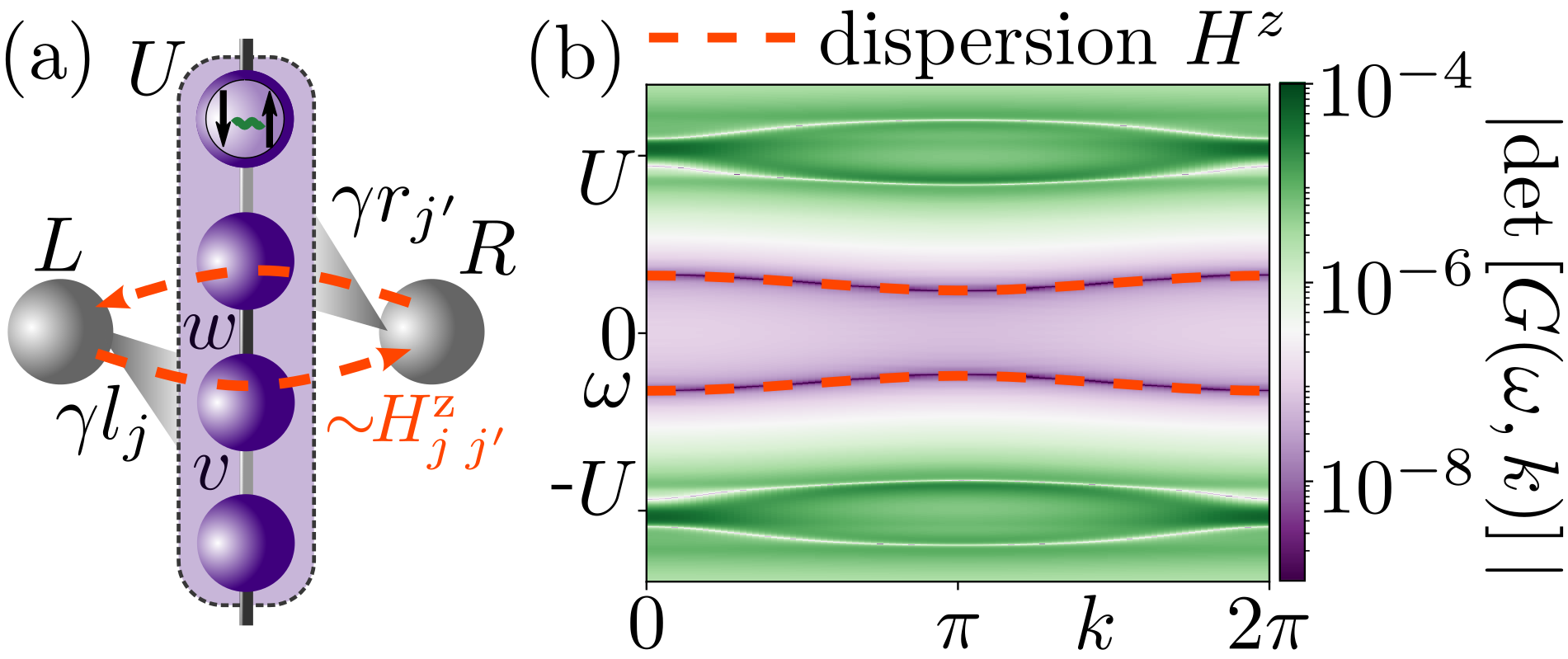
Figure 1: Cotunneling reveals GFZ Hamiltonian $H^{\text{z}}$: (a) Two spinful auxiliary sites $\{L,R\}$ weakly coupled by tunneling amplitudes $\{\gamma l_{j},\gamma r_{j^{\prime}}\}$ to a Hubbard system in Mott regime. Elastic cotunneling establishes an effective coupling between $L$ and $R$ (red, dashed line). (b) Numerical results (MPS) for the determinate of GF $|\text{det}[G(\omega,k)]|$: SSH-Hubbard model at half-filling with $N=60$ spinful sites, $v=0.75,w=1.0$, $U=10$, analytic prediction of the in-gap zero dispersion of $H^{\text{z}}$ (red, dashed line).

Here, we study co-tunneling through Mott insulators as a novel tool to reveal the shadow band structure of GFZ. As a setting (see Fig. 1 for an illustration), we propose a re-interpretation and generalization of the well-established experimental platform of co-tunneling measurements through quantum dots [9, 35, 36, 37, 38, 14, 39, 40, 41] by replacing a quantum dot in the Coulomb-blockade regime with a many-body system in a Mott phase that may even be engineered as a synthetic quantum material consisting of an array of coupled quantum dots [10, 9, 11]. We pinpoint two fundamental differences between our strongly correlated scenario and a tunneling probe for an uncorrelated band insulator. First, the band structure of GFZ appear in the numerator of the co-tunneling amplitude, contrary to an energy denominator for an uncorrelated insulator. Second, genuine correlation effects modify the zero-bands decisively as compared to the underlying free band structure of the Mott insulator. Using the striking example of topological distinction between zero-bands and the corresponding pole-bands, we demonstrate how these subtle fingerprints of many-body correlations can be directly observed through the co-tunneling amplitude.

Zeros band structure through perturbation theory

– To describe how to probe a solid-state system spectroscopically, we use the formalism of Green’s functions. At the one-particle level, this allows to quantify the response of the system upon adding or removing an electron, taking into account correlations effects. The single-particle electronic Green’s function in the Källén-Lehmann representation at zero temperature is explicitly dependent on the spectrum of excitations of the system [42, 43]:

$$G_{j,\sigma;j^{\prime},\sigma^{\prime}}(\omega) =\sum_{\nu}\Bigg{[}\frac{\langle GS|c_{j,\sigma}|E_{\nu}\rangle\langle E_{\nu}|c_{j^{\prime},\sigma^{\prime}}^{\dagger}|GS\rangle}{\omega+E_{GS}-E_{\nu}}$$

$$+\frac{\langle GS|c_{j^{\prime},\sigma^{\prime}}^{\dagger}|E_{\nu}\rangle\langle E_{\nu}|c_{j,\sigma}|GS\rangle}{\omega+E_{\nu}-E_{GS}}\Bigg{]}\text{.}$$ (1)

where $c^{(\dagger)}_{j,\sigma}$ denote the annihilation and creation operators for site $j$ and spin $\sigma$. In the non-interacting limit, the Hamiltonian and $G(\omega)$ are readily diagonalizable in a single-particle basis. The determination of the spectral and geometrical properties of the system then amounts to the study of the poles of $G(\omega)$, each of which represents an infinitely long-lived single-particle eigenmode. However, in presence of correlations, a large amount of matrix elements in the numerator become nonzero, reflecting the multitude of scattering events promoted by the many-body interaction term. As a result, the spectral weight distribution is broadened in the frequency-momentum plane. There is, however, a remarkable consequence of this scenario: in the spectral distribution, a set of isolated Green’s function zeros (GFZ) can emerge. Their presence has been linked to peculiar thermodynamic [44] and topological properties [25, 26, 33, 34, 27, 28, 29, 30, 31, 32], and the study of their dispersion is hence an intriguing, if nontrivial endeavor.

The GFZ are defined as zero eigenvalues of $G$, or equivalently as the points at which its determinant vanishes [25]. In the noninteracting limit, there are no isolated zeros. In the opposite case, where the system is deep in the Mott phase, two incoherent Hubbard bands form at high frequency, which contain the totality of the poles of the Green’s function, and a large number of zeros. However, inside the hard Mott gap between the two Hubbard bands no poles are present. By contrast, GFZ can and do manifest at low energy, irrespective of the system size. The focus of this work lies on how to detect these isolated in-gap GFZ which are entirely responsible for the low energy properties of the GF of Mott insulators [19, 20, 21, 22, 23, 24, 25, 26, 27, 28, 29, 30, 31, 32, 33, 34].

As a first step in our discussion, we derive a remarkably simple and intuitive expression for $G$ at low energies ($\omega\ll U$). Our non-interacting Hamiltonian $H_{0}=\sum h_{i\sigma;j\sigma^{\prime}}c^{\dagger}_{i,\sigma}c_{j,\sigma^{\prime}}$ consists of a linear combination of on-site terms, which we denote by $M$, and non-local hopping terms ($W$). The interaction term is of the Hubbard type $UH_{\text{int}}=2U\sum_{j}(n_{j,\downarrow}-\frac{1}{2})(n_{j,\uparrow}-\frac{1}{2})$, where $j$ labels the lattice site and $\sigma=\uparrow,\downarrow$ is the spin. The two competing energy scales are the bandwidth of $H_{0}$, $2D$ and the local Coulomb interaction strength $U$. In the half-filled Mott insulator, $U\gg D$. For convenience, we introduce the rescaled non-interacting Hamiltonian term $H^{\prime}_{0}=\frac{1}{D}H_{0}$, as well as the small parameter $\phi=\frac{D}{U}$. The Hamiltonian can therefore be rewritten as

$$H_{\text{H}}=U(\phi H^{\prime}_{0}+H_{\text{int}}).$$ (2)

In this form, $H_{\text{H}}$ naturally suggests a perturbative analysis in $\phi$: indeed, by applying degenerate perturbation theory [45] up to first order in $\phi$ we determine the perturbed eigenenergies eigenenergies $E_{\nu}^{P}$ and eigenstates $|E_{\nu}^{P}\rangle$, which we can then conveniently insert in Eq. (1) to obtain the perturbed Mott Green’s function. It is finally a matter of collecting all the lowest terms in $\phi$, to come to a key expression for the Green’s function which is valid at low energies $\omega\ll U$ :

$$G_{j,\sigma;j^{\prime},\sigma^{\prime}}(\omega)\underset{\omega,D\ll U}{\approx}\frac{1}{U^{2}}\left[-\omega\mathbb{I}+H^{\text{z}}\right]_{j,\sigma;j^{\prime},\sigma^{\prime}}+\mathcal{O}(\phi^{3}).$$ (3)

This expression is intuitively consistent with the strongly suppressed in-gap spectral distribution of a Mott insulator. More than that, it immediately and clearly highlights the presence, inside of the Mott gap, of points where the determinant of the Green’s function is exactly zero. These are the roots of the expression $H^{z}-\omega\mathbb{I}$. In other words, and inline with [33], we find that the low-energy isolated zeros of a Mott insulator are described by an effective Hamiltonian $H^{\text{z}}$. The detailed derivation of Eq. (3) can be found in the supplemental material [47].

Our approach is able to precisely characterize the effective Hamiltonian, and leads to a second interesting result about the GFZ: in this limit $H^{z}$ has, modulo some exactly quantifiable renormalization, the same form as the non-interacting term $H_{0}$ of the original Hamiltonian Eq. (2).

For strong Coulomb repulsion $U$ and at half-filling, the Hubbard model at low energies is well described by an effective spin-$1/2$ model [7, 8, 5, 6]. We can therefore rewrite the lowest-order terms in $G$ in the spin basis, thereby obtaining an expression linking the approximated Green’s function to spin-spin correlators, as derived in detail in [47]. For a $SU(2)$-symmetric groundstate and bare Hamiltonian $(H_{0})_{j,\sigma;j^{\prime},\sigma^{\prime}}=(M+W)_{jj^{\prime}}\delta_{\sigma,\sigma^{\prime}}$, we find a remarkably elegant expression for the effective Hamiltonian of the GFZ:

$$H^{\text{z}}_{jj^{\prime}}=M_{jj^{\prime}}\delta_{j,j^{\prime}}+4\langle\overrightarrow{S}_{j}\cdot\overrightarrow{S}_{j^{\prime}}\rangle_{j\neq j^{\prime}}W_{jj^{\prime}},$$ (4)

where $j,j^{\prime}$ are lattice sites. Here, expectation values are evaluated with respect to the groundstate eigenvector $|GS^{0}\rangle$ of the corresponding effective spin-$1/2$ model , and are hence accessible for a large variety of Hubbard models. A general discussion of $SU(2)$-breaking bare Hamiltonians is presented in [47], while we will restrict ourselves in the following to $SU(2)$-symmetric systems. The effective zeros Hamiltonian can then be decomposed in two terms, in a striking analogy with the on-site and hopping terms of the bare Hamiltonian $H_{0}$: (i) the on-site terms of the non-interacting Hamiltonian, described by $M$, are carried over in the dispersion of the zeros without renormalization, while (ii) the hopping terms, described by $W$, are re-scaled by the spin correlation function $\langle\overrightarrow{S}_{j}\cdot\overrightarrow{S}_{j^{\prime}}\rangle$ . This follows naturally from the combination of our perturbative approach around the atomic limit and the nature of competing energy scales in the system: any quadratic on-site term commutes with $H$ in the atomic limit, and the perturbed energy is just shifted by $M$ without renormalization. On the contrary, hopping and interaction strength are in direct competition: treating the first order perturbatively results in a lowest-order correction to the atomic limit Hamiltonian which famously depends on the spin-spin correlation function, as in the derivation of the superexchange [50, 51, 52, 8].

Probing the zeros

– As clearly evidenced by Eqs. (3) and (4), the knowledge of the zeros dispersion is sufficient to determine the spectral properties of the Mott system at low frequency. Obtaining a clear hint of the zeros’ behavior from experimental observations is instead less straightforward since any spectral measurement (e.g. via photoemission) would just give confirmation of the presence of a gap, without being able to resolve the elusive zeros within. We propose a novel approach to the problem which is, at the same time, surprisingly simple to implement: instead of directly performing spectroscopic measurements on the Mott insulator, we employ it as the potential barrier in a co-tunneling experiment, and study the effective coupling between the leads. We illustrate the setup via a minimal example, which is a convenient adaption of already existing quantum dot experimental setups [36, 11, 9, 10]. This is sketched in Fig.1 (a) and described by

$$H_{\text{tot}}=H_{\text{H}}+\gamma C+H_{\text{D}}$$ (5)

The system consists of two quantum dots, henceforth L and R, and a central tunneling medium. The Hamiltonian of the quantum dots, $H_{\text{D}}$, is that of a Hubbard atom with Coulomb repulsion $2U$, while the central element is a spin-isotropic Hubbard model in the Mott phase, described by the previously discussed Eq. (2). The chemical potential of the quantum dots is increased by $U$ in relation to the central Hubbard model, and independently adjustable by $\mu_{\text{L}},\mu_{\text{R}}$. The system-dot coupling $C$ is given by arbitrary hopping amplitudes $\{l_{i}\}$ and $\{r_{i}\}$ between the $i$-th site of the central Mott insulator and the L and R quantum dots. For simplicity, we will from now on omit the spin index $\sigma$, and restrict ourselves to the case where $l_{i}=\delta_{i,j}$ and $r_{i}=\delta_{i,j^{\prime}}$ for two sites $j\neq j^{\prime}$. The full derivation for the general case with arbitrary hopping array is provided in [47]. In a co-tunneling experiment, only the leads are directly probed. This amounts to tracing away the degrees of freedom associated to the central system, and only considering the overall propagation amplitude of excitation leaving (entering) the two leads via the quantum dots. These processes are, in our proposed setting, exactly described by the one-particle Green’s function of the central Mott insulator. If we are interested in the low-frequency excitations of the system, the picture can be simplified further, making use of the previously derived approximation for the Green’s function. In short, by applying two Schrieffer-Wolff transformations [53, 54, 55] in the limit of weak system-dot coupling $\gamma\ll D,U$, and assuming a large interaction $U$, we derive an effective spin-isotropic low energy Hamiltonian $\bar{h}$. It describes the dynamics of a single particle co-tunneling between the left and right quantum dots through the half-filled Mott-insulator:

$$\bar{h}=\begin{pmatrix}\mu_{\text{L}}+u_{\text{L}}(\mu_{\text{L}},\mu_{\text{R}})&t^{\ast}_{\text{co}}(\bar{\mu})\\ t_{\text{co}}(\bar{\mu})&\mu_{\text{R}}+u_{\text{R}}(\mu_{\text{L}},\mu_{\text{R}})\end{pmatrix}$$ (6)

where $\bar{\mu}$ is an “average” chemical potential $\frac{1}{2}\left(\mu_{\text{L}}+\mu_{\text{R}}\right)$. The presence of the central Mott insulator provides a renormalization to the on-site energies, given by $u_{L/R}\sim\mathcal{O}(\frac{\gamma^{2}}{U})$, which can be conveniently reabsorbed by tuning the quantum dot chemical potentials. The most relevant parameter in Eq. (6) is the amplitude

$$t_{\text{co}}(\bar{\mu})=\gamma^{2}G_{j,j^{\prime}}(\bar{\mu}),$$ (7)

which describes the co-tunneling mediated coupling between the left and right quantum dot via the central Mott insulator. We immediately to notice how, through Eq. (3), the co-tunneling amplitude $t_{\text{co}}$ is directly related to the GFZ-Hamiltonian $H^{\text{z}}$ of Eq.(4) via $t_{\text{co}}=\frac{\gamma^{2}}{U^{2}}\left(H^{\text{z}}\right)_{j,j^{\prime}}$. This clarifies the correspondence between the Mott Green’s function and the tunneling amplitude: instead of directly probing the features of the vanishing spectral function inside the Mott gap, a nearly impossible task, we are now recasting the same information into what is effectively a potential barrier for the evanescent wave of the co-tunneling experiment. Its features, and in particular the spectroscopically undetectable zeros, have a macroscopic effect on the measured occupations of the leads. As a further benefit, we can now take advantage of the well established theoretical tools and experimental techniques employed in the study of quantum tunneling, such as charge stability diagrams [56, 57, 58, 11, 59]and time-resolved charge detection of single tunneling events [60, 61, 62, 36].

Numerical results

– We now provide numerical evidence of our key findings by considering the paradigmatic case of the one-dimensional Su-Schrieffer-Heeger (SSH)-Hubbard model[33, 63], consisting of a bipartite chain with alternating hoppings $v$ and $w$, and arbitrary on-site potentials. We numerically solve the Hamiltonian of the co-tunneling setup by using a combination of Density Matrix Renormalization Group (DMRG) [64, 65], time-dependent variational principle (TDVP) [66, 67, 68] and exact diagonalization (ED) methods, by first computing the real time GF and then transforming it into the frequency domain, thus gaining access to the GFZ.

We first prove that our analytical formula for the zeros Hamiltonian is an adequate approximation of the in-gap spectral features of a Mott insulator. Fig.1 (b) shows a comparison between the determinant of the Green’s function of the SSH-Hubbard model, obtained via DMRG, and the approximated formula for the zeros effective Hamiltonian of Eq. (4). We note that the isolated zeros (dark purple regions of the color plot), which are formed in the Mott gap, are in perfect agreement with the eigenvalues of $H^{\text{z}}$ already at the intermediate value of $\phi\approx 1/10$.

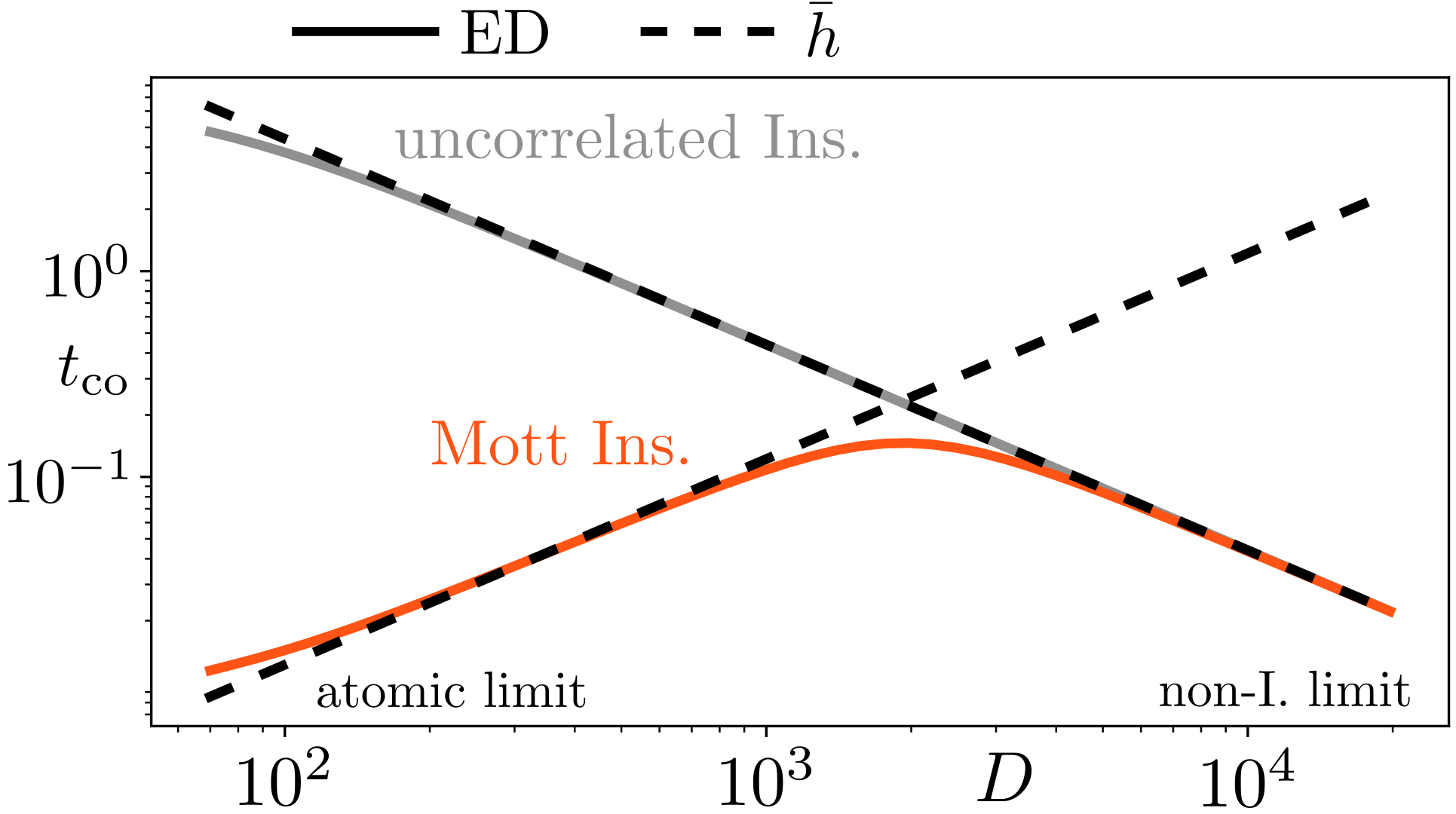
Figure 2: Co-tunneling amplitude $t_{\text{co}}$ as function of bandwidth $D$(fixed $U=2000$, $N=16$, $\gamma=20$,$l_{i}=\delta_{i,2}$,$r_{i}=\delta_{i,3}$, $v=0.9w$, PBC). SSH-Hubbard model (solid,red) shows linear $D$ dependence within the the Mott regime $\frac{D}{U}<1$, due to energy nominator in GF Eq.(3). Non-interacting insulator (solid,grey) with energy denominator (parameters as above but $U=0$). Analytical results, Eq.(7) (dashed).

We then turn our attention to the co-tunneling setup, numerically simulated by supplementing the quantum dots and coupling terms, $H_{\text{D}}$ and $C$, to the SSH-Hubbard Hamiltonian.

In Fig.2 we show the emergent co-tunneling amplitude for the experimental setup in Fig.1(a) between two interacting auxiliary quantum dots, as a function of the bandwidth $D$. We compare their behavior in the case of a Mott insulator and a conventional non-interacting insulator, and plot the two resulting curves (red and grey) as a function of $D$. The numerically obtained curves are to be compared with the two dashed lines, which show the two different behaviors in the non-interacting and Mott limits and can be extracted from Eq. (7). In the non-interacting limit, the behavior of the Green’s function $G$, as defined in Eq.(1), is determined by a single energy scale, the non-interacting bandwidth appearing at the denominator [42, 43]. Hence, $t_{\text{co}}\sim D^{-1}$, and the two solid lines are on top of each other and agree with the non-interacting behavior (negative slope in the logarithmic plot). At around $\frac{D}{U}\approx 1$, i.e. near the Mott transition, the behavior of the interacting system changes: now, the dominant energy scale of the system is the Coulomb interaction $U$, and approximation Eq. (3) holds. $H^{z}$, though renormalized as in Eq. (4), has a $\sim D$ dependence on the bandwidth, and the Mott co-tunneling amplitude indeed agrees with the positive-slope dashed line. The general agreement between the approximated value of $t_{\text{co}}$ and the numerically determined ones is remarkable, confirming the robustness of Eq.(7). Only at small bandwidth $D$ our co-tunneling approximation breaks down ($\gamma\approx D$) and higher order tunneling processes become relevant.

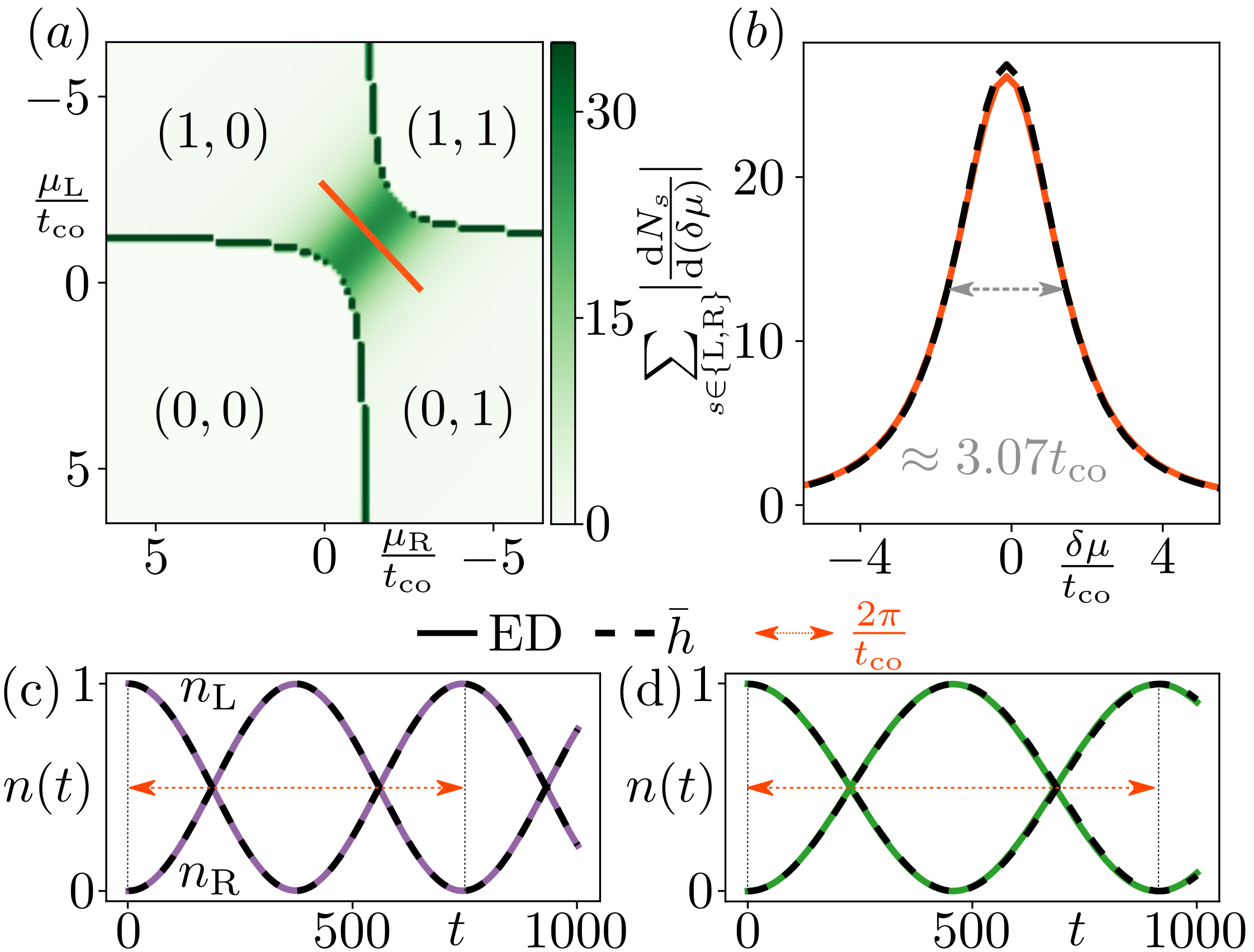
Figure 3: Charge stability diagram (ED, $U=200$ $N=16$, $\gamma=4$,$l_{i}=\delta_{i,2}$,$r_{i}=\delta_{i,3}$, $v=18$, $w=20$,PBC) : (a) Derivative particle number $N_{L}$($N_{R}$) on left(right) dot for varying potentials $\mu_{\text{L}},\mu_{\text{R}}$. In (b): cut through (a) (red line), FWHM is proportional to co-tunneling $t_{\text{co}}$. (c) and (d): charge oscillations between aux. dots (initial localization left dot) same parameter as (a), but OBC, $N=20$, $l_{i}=\delta_{i,1}$,$r_{i}=\delta_{i,2}$ in (c) and $l_{i}=\delta_{i,3}$,$r_{i}=\delta_{i,4}$ in (d). Analytical results (dashed) from Eq.(7).

Our co-tunneling approach to detecting Green’s function zeros can be nicely illustrated with the well established tool of charge-stability diagrams [56, 57, 58, 11, 59], which is commonly used to describe the behavior of quantum dots as a function of control voltages. In Fig.3 (a) we show the charge-stability diagram of our co-tunneling setup, by plotting the derivative of the charge occupation $N_{L/R}$ with respect to the detuning $\delta\mu=\mu_{\text{L}}-\mu_{\text{R}}$ at varying chemical potentials $\mu_{\text{L}},\mu_{\text{R}}$. Due to the finite tunneling amplitude $t_{\text{co}}$, the boundaries of the characteristic checkerboard structure of the uncoupled system ($\gamma=0$) are smeared out and and the localization of a single particle can be tuned smoothly from the left dot $(1,0)$ to the right dot $(0,1)$. Fig.3 (b) shows a diagonal cut through Fig.3 (a) at a fixed average potential $\bar{\mu}=\frac{1}{2}\left(\mu_{\text{L}}+\mu_{\text{R}}\right)$ (red line). The FWHM of the Lorentzian dispersion is directly proportional to the co-tunneling amplitude. An alternative way of probing the co-tunneling amplitude is to measure the frequency of Rabi-charge oscillations between the dots [60, 61, 62, 36], which can be extracted by the time-evolution of a localized state and compared with the theoretical value $\Omega\approx\sqrt{|t_{\text{co}}|^{2}+\omega^{2}_{D}}$, where $\omega_{D}\approx\frac{1}{2}\delta\mu+\mathcal{O}(\frac{\gamma^{2}}{U})$ is a shifted detuning between the two quantum dots, easily controllable via $\mu_{L}$ and $\mu_{R}$. In Fig.3 (c) and (d) we plot the numerically calculated time-dependent charge occupation values of the two quantum dots on resonance $\omega_{D}=0$ (at peak maximum in Fig.3 (b)), when the system is initialized in the completely localized (1,0)-state. The data are in perfect agreement with the predicted oscillation frequency, which can be easily extracted by Eq.(6). In a real experiment, the perturbative limit $\frac{\gamma}{D}\ll\frac{D}{U}\ll 1$, may not be perfectly accessible and is further inherently tied to an small co-tunneling amplitude, making it experimentally challenging. Despite this limitation, macroscopic values of $t_{\text{co}}$ ($\geq 0.5\mu eV$) can still be achieved for a broad range of typical parameters $U,D$ and $\gamma$, within an acceptable quantitative deviation ($\leq 10\%$) from the effective Hamiltonian $\bar{h}$ (see [47] for details). Interestingly, we also find that the striking spin renormalization in Eq.(4) can be probed qualitatively, without requiring fine-tuning of the dots. More specifically, we find a notable amplification of the tunneling amplitude as function of varying boundary conditions as a characteristic signature of the spin-spin correlations (see [47] for further details).

Conclusion

– Starting from a degenerate perturbation theory around the atomic limit, we have derived a simple yet highly accurate approximation for the low-frequency features of a Mott Green’s function, which can be completely described by a dispersion relation for the Green’s function zeros. This situation is reminiscent of a non-interacting system with the important distinction that the effective dispersion of zeros appears in the numerator of the Green’s functions, and is renormalized compared to the underlying free band structure by means of spin correlators, as we have quantified. Our main result is the establishment of a direct link between the dispersion of zeros and the transmission amplitude naturally probed in a co-tunneling experiment, which drastically simplifies the task of observing and characterizing Green’s function zeros. We have provided extensive numerical proof of the correctness and resilience of our approximation, and suggested a feasible experimental setup for the verification of our key findings. Numerical simulations suggest that the fingerprints of the zeros dispersion and renormalization are observable already for small systems: specifically, an ensemble of six quantum dots (2 leads and 4 in the central Hubbard tunneling medium) is already sufficient to quantify an interesting correlation induced renormalization of band parameters.

Acknowledgments

– We acknowledge financial support from the German Research Foundation (DFG) through the Collaborative Research Centre SFB 1143 (Project-ID 247310070), the Cluster of Excellence ct.qmat (Project-ID 390858490). Our numerical calculations have been performed at the Center for Information Services and High Performance Computing (ZIH) at TU Dresden.

Appendix A Perturbation theory for the Green’s function

In the following section we derive the GF for the Hubbard model within the strongly correlated limit $\frac{D}{U}\rightarrow 0$ , i.e., deep in the Mott regime. The general Hubbard Hamiltonian is given as:

$$H_{\text{H}} =H_{0}+UH_{\text{int}}=D\phi^{-1}\left(\phi H^{\prime}_{0}+H_{\text{int}}\right)$$ (8)

$$H_{\text{int}} =2\sum_{j,\alpha}(n_{j,\downarrow}-\frac{1}{2})(n_{j,\uparrow}-\frac{1}{2})\text{,}$$ (9)

where the non-interacting Hamiltonian $H_{0}=\sum c^{\dagger}_{j,\sigma}h_{j,\sigma;j^{\prime},\sigma^{\prime}}c_{j^{\prime},\sigma^{\prime}}$ is quadratic in its creation(annihilation) operators $c^{\dagger}_{j,\sigma}$ ($c_{j,\sigma}$) and obeys the bandwidth $2D$. The Hubbard interaction $H_{\text{int}}$ consists on the local density operators $n_{j,\sigma}=c^{\dagger}_{j,\sigma}c_{j,\sigma}$, acting on the spinful lattice sites $j$.

Deep in the Mott regime, Eq.(8) implies an perturbative expansion [45] of the eigenstates in $\phi=\frac{D}{U}$, where the rescaled bare Hamiltonian $H^{\prime}_{0}=\frac{1}{D}H_{0}$ acts as perturbation. Then, we insert the resulting expanded eigenstates and eigenenergies into the Källen-Lehmann representation and eventually collect all terms up to the second order. Thereby, we will first derive an rescaled GF $G^{\prime}(\phi\frac{\omega}{D})=\frac{D}{\phi}G(\omega)$, where $G^{\prime}$ denotes the GF corresponding to the Hamiltonian $D^{-1}\phi H_{\text{H}}$, afterwards we can easily readout $G(\omega)$.

A.1 Eigenvector structure towards the strongly correlated limit

The Hubbard interaction $H_{\text{int}}$ towards strong correlation $\phi\rightarrow 0$ avoids empty and double occupied sites, i.e., they cost an energy amount of $2D\phi^{-1}=2U$ . The eigenenergies will then arrange in well separated energy sectors according the amount of empty and double occupied sides (see Fig.4). We will expand the eigenstates around this strongly correlated limit, hence for house-holding reasons we will index-labelling all the unperturbed eigenstates $\{|E^{0,m}_{\nu,l}\rangle\}$ according to their energy sectors. In the following we denote by $m=N-N_{h}$ the relative particle number, with the total particle number $N=\sum_{j,\sigma}n_{j,\sigma}$ and the particle number at half-filling $N_{h}$. Furthermore, by $l$ we count the empty or double occupied sites additional to the lowest energy state of the corresponding particle sector $m$. In combination, the indices $l$ and $m$ fully determine the energy of each eigenstate in the atomic limit:

$$E^{0,m}_{\nu,l}=E_{0}+U(|m|+2l)\text{.}$$ (10)

Here $E_{0}=-\frac{U}{2}N_{s}$ denotes a global offset, with the number of all spinful sites $N_{s}$. The last index $\nu$ differentiates between the additional degenerated eigenstates within a particle sector $m,l$.

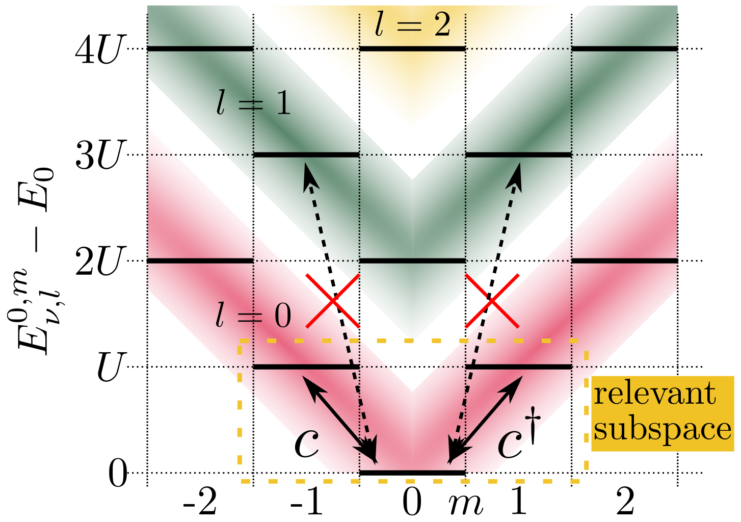
Figure 4: Energy levels $E^{0,m}_{\nu,l}=E_{0}+U(|m|+2l)$ for a typical Hubbard system in the Mott regime (atomic limit): all eigenstates can be sorted with respect to the particle-number deviation from half-filling $N=N_{h}+m$ and the amount of empty(douple occupied) sites $l$ additional to the lowest states for a fixed particle-number sector (coloured regions). For each energy there is a huge degeneracy denoted by $\nu$. The energy $E_{0}$ denotes the lowest global energy. In order to get the zero temperature GF the only relevant subspace consist of the global groundstate and the lowest energy sector with $m=|1|,l=0$ (yellow box). Direct Scattering from the groundstate into higher energies with $l>0$ is forbidden within the atomic limit (black arrows).

A.2 Decomposition of the non-interacting Hamiltonian

The bare hopping $H_{0}$ contains various terms which can be resorted with respect to the energy-increase regarding the strongly interacting limit,i.e., their ability to produce empty and double-occupied sites by acting on the groundstate at half-filling $H_{0}|GS_{0}\rangle$.

$$H_{0}=\sum_{l}H_{0,l}$$ (11)

Here $H_{0,l}$ scatters the groundstate $|GS_{0}\rangle$ into the energy level $l$ within the half-filled particle sector $m=0$.

For the generic Hubbard model there are only local terms $H_{0,l=0}$($\equiv M$ in the letter), like on-site potentials and spin-flip terms, and non-local terms $H_{0,l=1}$($\equiv W$ in the letter), e.g., site-to-site hopping terms.

A.3 First order perturbation theory

As first step we formally expand the perturbed eigenstates(-energies) $|E^{P,m}_{\nu,l}\rangle$($E^{P,m}_{\nu,l}$) of $\frac{\phi}{D}H_{\text{H}}$ in Eq.(8) towards the unperturbed limit, up to the first order in $\phi$. This is essentially standard degenerated perturbation theory [45] and maps the atomic eigenstates(-energies) $|E^{0,m}_{\nu,l}\rangle$($E^{0,m}_{\nu,l}$) smoothly to the perturbed ones.

$$E^{P,m}_{\nu,l} \approx E^{0,m}_{\nu,l}+\phi\langle E^{0,m}_{\nu,l}|H^{\prime}_{0}|E^{0,m}_{\nu,l}\rangle+\mathcal{O}(\phi^{2})$$ (12)

$$|E^{P,m}_{\nu,l}\rangle \approx|E^{0,m}_{\nu,l}\rangle+\phi\sum_{l^{\prime}\neq l}\frac{P_{l^{\prime}}^{m}H^{\prime}_{0}|E^{0,m}_{\nu,l}\rangle}{2(l-l^{\prime})}+\mathcal{O}(\phi^{2})$$ (13)

$$P_{l^{\prime}}^{m} =\sum_{\nu^{\prime}}|E^{0,m}_{\nu^{\prime},l^{\prime}}\rangle\langle E^{0,m}_{\nu^{\prime},l^{\prime}}|$$

Here, we introduce the energy-sector projector $P_{l}^{m}$. It is important to note that the degeneracy within each sector $(m,l)$, denoted by $\nu$, must, in principle, be resolved by applying non-trivial higher-order perturbation theory [45]. However, for the final result, it suffices that such an expansion exists. Moreover, Eq. (13) can be interpreted as an inverse Schrieffer-Wolff transformation [53, 55, 54], which maps the eigenstates of an effective model defined in the atomic limit back to the original basis.

Let’s insert the perturbed eigenstates(-energies) Eq.(13) into the Källen-Lehmann representation:

$$G^{\prime}_{j,\sigma;j^{\prime},\sigma^{\prime}}(\phi\omega^{\prime}) =\sum_{\nu,l}\Bigg{[}\frac{\left<GS^{P}|c_{j,\sigma}|E_{\nu,l}^{P,+}\right>\left<E_{\nu,l}^{P,+}|c^{\dagger}_{j^{\prime},\sigma^{\prime}}|GS^{P}\right>}{\phi\omega^{\prime}+E_{0}^{P}-E_{\nu,l}^{P,+}}+\frac{\left<E_{\nu,l}^{P,-}|c_{j,\sigma}|GS^{P}\right>\left<GS^{P}|c^{\dagger}_{j^{\prime},\sigma^{\prime}}|E_{\nu,l}^{P,-}\right>}{\phi\omega^{\prime}+E_{\nu,l}^{P,-}-E_{0}^{P}}\Bigg{]}$$

$$=\sum_{\nu,l}\Bigg{[}\frac{A_{j,\sigma;j^{\prime},\sigma^{\prime}}^{\nu,l}}{\phi\omega^{\prime}+E_{0}^{P}-E_{\nu,l}^{P,+}}+\frac{B_{j,\sigma;j^{\prime},\sigma^{\prime}}^{\nu,l}}{\phi\omega^{\prime}+E_{\nu,l}^{P,-}-E_{0}^{P}}\Bigg{]}\text{.}$$ (14)

We already rescaled the frequency $\phi\omega^{\prime}$, where $\omega^{\prime}=\frac{\omega}{D}$. We find for the expanded $A_{j,\sigma;j^{\prime},\sigma^{\prime}}^{\nu,l}$:

$$A_{j,\sigma;j^{\prime},\sigma^{\prime}}^{\nu,l} =\langle GS^{P}|c_{j,\sigma}|E^{P,+}_{\nu,l}\rangle\langle E^{P,+}_{\nu,l}|c^{\dagger}_{j^{\prime},\sigma^{\prime}}|GS^{P}\rangle$$

$$\approx\langle GS^{0}|\left(1-\sum_{k>0}\frac{\phi}{2k}H^{\prime}_{0}P^{0}_{k}\right)c_{j,\sigma}\left(1+\sum_{l^{\prime}\neq l}\frac{\phi}{2(l-l^{\prime})}P^{+}_{l}H^{\prime}_{0}\right)|E^{0,+}_{\nu,l}\rangle$$

$$\times\langle E^{0,+}_{\nu,l}|\left(1+\sum_{l^{\prime}\neq l}\frac{\phi}{2(l-l^{\prime})}H^{\prime}_{0}P^{+}_{l}\right)c^{\dagger}_{j^{\prime},\sigma^{\prime}}\left(1-\sum_{k>0}\frac{\phi}{2k}P^{0}_{k}H^{\prime}_{0}\right)|GS^{0}\rangle$$

$$\approx\langle GS^{0}|c_{j,\sigma}+\phi\left[-\sum_{k>0}\frac{1}{2k}H^{\prime}_{0}P^{0}_{k}c_{j,\sigma}+c_{j,\sigma}\sum_{l^{\prime}\neq l}\frac{1}{2(l-l^{\prime})}P^{+}_{l^{\prime}}H^{\prime}_{0}\right]|E^{0,+}_{\nu,l}\rangle$$

$$\times\langle E^{0,+}_{\nu,l}|c^{\dagger}_{j^{\prime},\sigma^{\prime}}+\phi\left[\sum_{l^{\prime}\neq l}\frac{1}{2(l-l^{\prime})}H^{\prime}_{0}P^{+}_{l^{\prime}}c^{\dagger}_{j^{\prime},\sigma^{\prime}}-c^{\dagger}_{j^{\prime},\sigma^{\prime}}\sum_{k>0}\frac{1}{2k}P^{0}_{k}H^{\prime}_{0}\right]|GS^{0}\rangle$$

$$\approx\langle GS^{0}|c_{j,\sigma}|E^{0,+}_{\nu,l}\rangle\langle E^{0,+}_{\nu,l}|c^{\dagger}_{j^{\prime},\sigma^{\prime}}|GS^{0}\rangle+\phi\langle GS^{0}|c_{j,\sigma}|E^{0,+}_{\nu,l}\rangle\langle E^{0,+}_{\nu,l}|\sum_{l^{\prime}\neq l}\frac{1}{2(l-l^{\prime})}H^{\prime}_{0}P^{+}_{l^{\prime}}c^{\dagger}_{j^{\prime},\sigma^{\prime}}|GS^{0}\rangle$$

$$-\phi\langle GS^{0}|c_{j,\sigma}|E^{0,+}_{\nu,l}\rangle\langle E^{0,+}_{\nu,l}|c^{\dagger}_{j^{\prime},\sigma^{\prime}}\sum_{k>0}\frac{1}{2k}P^{0}_{k}H^{\prime}_{0}|GS^{0}\rangle-\phi\langle GS^{0}|\sum_{k>0}\frac{1}{2k}H^{\prime}_{0}P^{0}_{k}c_{j,\sigma}|E^{0,+}_{\nu,l}\rangle\langle E^{0,+}_{\nu,l}|c^{\dagger}_{j^{\prime},\sigma^{\prime}}|GS^{0}\rangle$$

$$+\phi\langle GS^{0}|c_{j,\sigma}\sum_{l^{\prime}\neq l}\frac{1}{2(l-l^{\prime})}P^{+}_{l^{\prime}}H^{\prime}_{0}|E^{0,+}_{\nu,l}\rangle\langle E^{0,+}_{\nu,l}|c^{\dagger}_{j^{\prime},\sigma^{\prime}}|GS^{0}\rangle$$

$$=A_{j,\sigma;j^{\prime},\sigma^{\prime}}^{0,\nu,l=0}+\frac{\phi}{2}A_{j,\sigma;j^{\prime},\sigma^{\prime}}^{1,\nu,l=0}+\mathcal{O}(\phi^{2})$$ (15)

Only the lowest energy subspace with $l=0$ is relevant for our expansion, since terms like $\langle GS^{0}|c_{j,\sigma}|E^{0,+}_{\nu,l}\rangle,\langle E^{0,+}_{\nu,l}|c^{\dagger}_{j,\sigma}|GS^{0}\rangle$ are subspace conserving. Similar we find for $B_{j,\sigma;j^{\prime},\sigma^{\prime}}^{\nu,l}$:

$$B_{j,\sigma;j^{\prime},\sigma^{\prime}}^{\nu,l} =\langle GS^{P}|c^{\dagger}_{j^{\prime},\sigma^{\prime}}|E^{P,-}_{\nu,l}\rangle\langle E^{P,-}_{\nu,l}|c_{j,\sigma}|GS^{P}\rangle$$

$$\approx\langle GS^{0}|\left(1-\sum_{k>0}\frac{\phi}{2k}H^{\prime}_{0}P^{0}_{k}\right)c^{\dagger}_{j^{\prime},\sigma^{\prime}}\left(1+\sum_{l^{\prime}\neq l}\frac{\phi}{2(l-l^{\prime})}P^{-}_{l}H^{\prime}_{0}\right)|E^{0,-}_{\nu,l}\rangle$$

$$\times\langle E^{0,-}_{\nu,l}|\left(1+\sum_{l^{\prime}\neq l}\frac{\phi}{2(l-l^{\prime})}H^{\prime}_{0}P^{-}_{l}\right)c_{j,\sigma}\left(1-\sum_{k>0}\frac{\phi}{2k}P^{0}_{k}H^{\prime}_{0}\right)|GS^{0}\rangle$$

$$\approx\langle GS^{0}|c^{\dagger}_{j^{\prime},\sigma^{\prime}}+\phi\left[-\sum_{k>0}\frac{1}{2k}H^{\prime}_{0}P^{0}_{k}c^{\dagger}_{j^{\prime},\sigma^{\prime}}+c^{\dagger}_{j^{\prime},\sigma^{\prime}}\sum_{l^{\prime}\neq l}\frac{1}{2(l-l^{\prime})}P^{-}_{l^{\prime}}H^{\prime}_{0}\right]|E^{0,-}_{\nu,l}\rangle$$

$$\times\langle E^{0,-}_{\nu,l}|c_{j,\sigma}\phi\left[\sum_{l^{\prime}\neq l}\frac{1}{2(l-l^{\prime})}H^{\prime}_{0}P^{-}_{l^{\prime}}c_{j,\sigma}-c_{j,\sigma}\sum_{k>0}\frac{1}{2k}P^{0}_{k}H^{\prime}_{0}\right]|GS^{0}\rangle$$

$$\approx\langle GS^{0}|c^{\dagger}_{j^{\prime},\sigma^{\prime}}|E^{0,-}_{\nu,l}\rangle\langle E^{0,-}_{\nu,l}|c_{j,\sigma}|GS^{0}\rangle$$

$$+\phi\langle GS^{0}|c^{\dagger}_{j^{\prime},\sigma^{\prime}}|E^{0,-}_{\nu,l}\rangle\langle E^{0,-}_{\nu,l}|\sum_{l^{\prime}\neq l}\frac{1}{2(l-l^{\prime})}H^{\prime}_{0}P^{-}_{l^{\prime}}c_{j,\sigma}|GS^{0}\rangle+\phi\langle GS^{0}|c^{\dagger}_{j^{\prime},\sigma^{\prime}}\sum_{l^{\prime}\neq l}\frac{1}{2(l-l^{\prime})}P^{-}_{l^{\prime}}H^{\prime}_{0}|E^{0,-}_{\nu,l}\rangle\langle E^{0,-}_{\nu,l}|c_{j,\sigma}|GS^{0}\rangle$$

$$-\phi\langle GS^{0}|c^{\dagger}_{j^{\prime},\sigma^{\prime}}|E^{0,-}_{\nu,l}\rangle\langle E^{0,-}_{\nu,l}|c_{j,\sigma}\sum_{k>0}\frac{1}{2k}P^{0}_{k}H^{\prime}_{0}|GS^{0}\rangle-\phi\langle GS^{0}|\sum_{k>0}\frac{1}{2k}H^{\prime}_{0}P^{0}_{k}c^{\dagger}_{j^{\prime},\sigma^{\prime}}|E^{0,-}_{\nu,l}\rangle\langle E^{0,-}_{\nu,l}|c_{j,\sigma}|GS^{0}\rangle$$

$$=B_{j,\sigma;j^{\prime},\sigma^{\prime}}^{0,\nu,l=0}+\frac{\phi}{2}B_{j,\sigma;j^{\prime},\sigma^{\prime}}^{1,\nu,l=0}+\mathcal{O}(\phi^{2})$$ (16)

As next step, we expand the energies in the corresponding denominators with Eq.(12):

$$\frac{1}{\phi\omega^{\prime}+E^{P}_{0}-E^{P,+}_{\nu,l}}\approx\frac{1}{\phi\omega^{\prime}-1-2l+\phi\langle GS^{0}|H^{\prime}_{0}|GS^{0}\rangle-\phi\langle E^{0,+}_{\nu,l}|H^{\prime}_{0}|E^{0,+}_{\nu,l}\rangle}\text{.}$$ (17)

Similarly, we get the second denominator:

$$\frac{1}{\phi\omega^{\prime}-E^{P}_{0}+E^{P,-}_{\nu,l}}\approx\frac{1}{\phi\omega^{\prime}+1+2l-\phi\langle GS^{0}|H^{\prime}_{0}|GS^{0}\rangle+\phi\langle E^{0,-}_{\nu,l}|H^{\prime}_{0}|E^{0,-}_{\nu,l}\rangle}\text{.}$$ (18)

Then, we expand the denominators at $\phi=0$. Notice that $l=0$ due to Eq.(15) and Eq.(16):

$$\frac{A_{j,\sigma;j^{\prime},\sigma^{\prime}}^{\nu,0}}{\phi\omega^{\prime}+E^{P}_{0}-E^{P,+}_{\nu,0}}\approx-A_{j,\sigma;j^{\prime},\sigma^{\prime}}^{0,\nu,0}+\frac{\phi}{2}\left[-A_{j,\sigma;j^{\prime},\sigma^{\prime}}^{1,\nu,0}-2A_{j,\sigma;j^{\prime},\sigma^{\prime}}^{0,\nu,0}\left(\omega^{\prime}+\langle GS^{0}|H^{\prime}_{0}|GS^{0}\rangle-\langle E^{0,+}_{\nu,0}|H^{\prime}_{0}|E^{0,+}_{\nu,0}\rangle\right)\right]+\mathcal{O}(\phi^{2})\text{,}$$ (19)

$$\frac{B_{j,\sigma;j^{\prime},\sigma^{\prime}}^{\nu,0}}{\phi\omega^{\prime}-E^{P}_{0}+E^{P,-}_{\nu,0}}\approx B_{j,\sigma;j^{\prime},\sigma^{\prime}}^{0,\nu,0}+\frac{\phi}{2}\left[B_{j,\sigma;j^{\prime},\sigma^{\prime}}^{1,\nu,0}+2B_{j,\sigma;j^{\prime},\sigma^{\prime}}^{0,\nu,0}\left(-\omega^{\prime}+\langle GS^{0}|H^{\prime}_{0}|GS^{0}\rangle-\langle E^{0,-}_{\nu,0}|H^{\prime}_{0}|E^{0,-}_{\nu,0}\rangle\right)\right]+\mathcal{O}(\phi^{2})\text{.}$$ (20)

The last step involves expanding a rational function, which is valid only for frequencies $|\omega^{\prime}|\ll 1$, i.e., well within the Mott gap. Otherwise, performing this expansion near a pole would result in significant errors. Including the summation in Eq.14 we can simplify each term even further:

$$-\sum_{\nu}A_{j,\sigma;j^{\prime},\sigma^{\prime}}^{0,\nu,0} =-\sum_{\nu}\langle GS^{0}|c_{j,\sigma}|E^{0,+}_{\nu,0}\rangle\langle E^{0,+}_{\nu,0}|c_{j^{\prime},\sigma^{\prime}}^{\dagger}|GS^{0}\rangle=-\langle GS^{0}|c_{j,\sigma}c_{j^{\prime},\sigma^{\prime}}^{\dagger}|GS^{0}\rangle\text{ ,}$$ (21)

$$-\sum_{\nu}A_{j,\sigma;j^{\prime},\sigma^{\prime}}^{1,\nu,0} =\sum_{\nu}\langle GS^{0}|c_{j,\sigma}|E^{0,+}_{\nu,0}\rangle\langle E^{0,+}_{\nu,0}|\sum_{l^{\prime}\neq 0}\frac{1}{l^{\prime}}H^{\prime}_{0}P^{+}_{l^{\prime}}c_{j^{\prime},\sigma^{\prime}}^{\dagger}+c_{j^{\prime},\sigma^{\prime}}^{\dagger}\sum_{k>0}\frac{1}{k}P^{0}_{k}H^{\prime}_{0}|GS^{0}\rangle$$

$$+\langle GS^{0}|\sum_{k>0}\frac{1}{k}H^{\prime}_{0}P^{0}_{k}c_{j,\sigma}+c_{j,\sigma}\sum_{l^{\prime}\neq 0}\frac{1}{l^{\prime}}P^{+}_{l^{\prime}}H^{\prime}_{0}|E^{0,+}_{\nu,0}\rangle\langle E^{0,+}_{\nu,0}|c_{j^{\prime},\sigma^{\prime}}^{\dagger}|GS^{0}\rangle$$

$$=\langle GS^{0}|c_{j,\sigma}c_{j^{\prime},\sigma^{\prime}}^{\dagger}\sum_{k>0}\frac{1}{k}P^{0}_{k}H^{\prime}_{0}|GS^{0}\rangle+\langle GS^{0}|H^{\prime}_{0}\sum_{k>0}\frac{1}{k}P^{0}_{k}c_{j,\sigma}c_{j^{\prime},\sigma^{\prime}}^{\dagger}|GS^{0}\rangle$$

$$=\sum_{k>0}\frac{1}{k}\langle GS^{0}|\left[c_{j,\sigma}c_{j^{\prime},\sigma^{\prime}}^{\dagger},H^{\prime}_{0,k}\right]_{+}|GS^{0}\rangle\text{ ,}$$ (22)

$$\sum_{\nu}A_{j,\sigma;j^{\prime},\sigma^{\prime}}^{0,\nu,0}\langle E^{0,+}_{\nu,0}|H^{\prime}_{0}|E^{0,+}_{\nu,0}\rangle =\sum_{\nu}\langle GS^{0}|c_{j,\sigma}|E^{0,+}_{\nu,0}\rangle\langle E^{0,+}_{\nu,0}|c_{j^{\prime},\sigma^{\prime}}^{\dagger}|GS^{0}\rangle\langle E^{0,+}_{\nu,0}|H^{\prime}_{0}|E^{0,+}_{\nu,0}\rangle$$

$$=\langle GS^{0}|c_{j,\sigma}H^{\prime}_{0}c_{j^{\prime},\sigma^{\prime}}^{\dagger}|GS^{0}\rangle\text{.}$$ (23)

We find similar results for the $B$-terms:

$$\sum_{\nu}B_{j,\sigma;j^{\prime},\sigma^{\prime}}^{0,\nu,0} =\sum_{\nu}\langle GS^{0}|c_{j^{\prime},\sigma^{\prime}}^{\dagger}|E^{0,-}_{\nu,0}\rangle\langle E^{0,-}_{\nu,0}|c_{j,\sigma}|GS^{0}\rangle=\langle GS^{0}|c_{j^{\prime},\sigma^{\prime}}^{\dagger}c_{j,\sigma}|GS^{0}\rangle\text{ ,}$$ (24)

$$\sum_{\nu}B_{j,\sigma;j^{\prime},\sigma^{\prime}}^{1,\nu,0} =-\sum_{\nu}\langle GS^{0}|c_{j^{\prime},\sigma^{\prime}}^{\dagger}|E^{0,-}_{\nu,0}\rangle\langle E^{0,-}_{\nu,0}|\sum_{l^{\prime}\neq 0}\frac{1}{l^{\prime}}H^{\prime}_{0}P^{-}_{l^{\prime}}c_{j,\sigma}+c_{j,\sigma}\sum_{k>0}\frac{1}{k}P^{0}_{k}H^{\prime}_{0}|GS^{0}\rangle$$

$$-\sum_{\nu}\langle GS^{0}|\sum_{k>0}\frac{1}{k}H^{\prime}_{0}P^{0}_{k}c_{j^{\prime},\sigma^{\prime}}^{\dagger}+c_{j^{\prime},\sigma^{\prime}}^{\dagger}\sum_{l^{\prime}\neq 0}\frac{1}{l^{\prime}}P^{-}_{l^{\prime}}H^{\prime}_{0}|E^{0,-}_{\nu,0}\rangle\langle E^{0,-}_{\nu,0}|c_{j,\sigma}|GS^{0}\rangle$$

$$=-\sum_{k>0}\frac{1}{k}\langle GS^{0}|\left[c_{j^{\prime},\sigma^{\prime}}^{\dagger}c_{j,\sigma},H^{\prime}_{0,k}\right]_{+}|GS^{0}\rangle\text{ ,}$$ (25)

$$\sum_{\nu}B_{j,\sigma;j^{\prime},\sigma^{\prime}}^{0,\nu,0}\langle E^{0,-}_{\nu,0}|H^{\prime}_{0}|E^{0,-}_{\nu,0}\rangle =\sum_{\nu}\langle GS^{0}|c_{j^{\prime},\sigma^{\prime}}^{\dagger}|E^{0,-}_{\nu,0}\rangle\langle E^{0,-}_{\nu,0}|c_{j,\sigma}|GS^{0}\rangle\langle E^{0,-}_{\nu,0}|H^{\prime}_{0}|E^{0,-}_{\nu,0}\rangle$$

$$=\langle GS^{0}|c_{j^{\prime},\sigma^{\prime}}^{\dagger}H^{\prime}_{0}c_{j,\sigma}|GS^{0}\rangle\text{.}$$ (26)

All terms together: Eq.(14), Eq.(19),Eq.(20), Eq.(21), Eq.(22), Eq.(23), Eq.(24), Eq.(25), Eq.(26), result in the first order approximation of the GF:

$$G^{\prime}_{j,\sigma;j^{\prime},\sigma^{\prime}}(\phi\omega^{\prime}) \approx\left(G^{\prime}_{0}\right)_{j,\sigma;j^{\prime},\sigma^{\prime}}+\phi\left(G^{\prime}_{1}\right)_{j,\sigma;j^{\prime},\sigma^{\prime}}-\phi\omega^{\prime}+\mathcal{O}(\phi^{2})$$ (27)

$$\left(G^{\prime}_{0}\right)_{j,\sigma;j^{\prime},\sigma^{\prime}} =\langle GS^{0}|c_{j^{\prime},\sigma^{\prime}}^{\dagger}c_{j,\sigma}|GS^{0}\rangle-\langle GS^{0}|c_{j,\sigma}c_{j^{\prime},\sigma^{\prime}}^{\dagger}|GS^{0}\rangle$$ (28)

$$\left(G^{\prime}_{1}\right)_{j,\sigma;j^{\prime},\sigma^{\prime}} =\sum_{k>0}\frac{1}{2k}\left[\langle GS^{0}|\left[c_{j,\sigma}c_{j^{\prime},\sigma^{\prime}}^{\dagger},H^{\prime}_{0,k}\right]_{+}|GS^{0}\rangle-\langle GS^{0}|\left[c_{j^{\prime},\sigma^{\prime}}^{\dagger}c_{j,\sigma},H^{\prime}_{0,k}\right]_{+}|GS^{0}\rangle\right]$$

$$\quad+\left[\langle GS^{0}|c_{j,\sigma}(H^{\prime}_{0}-\Delta^{\prime}_{0})c_{j^{\prime},\sigma^{\prime}}^{\dagger}|GS^{0}\rangle-\langle GS^{0}|c_{j^{\prime},\sigma^{\prime}}^{\dagger}(H^{\prime}_{0}-\Delta^{\prime}_{0})c_{j,\sigma}|GS^{0}\rangle\right]$$ (29)

$$\Delta^{\prime}_{0} =\langle GS^{0}|H^{\prime}_{0}|GS^{0}\rangle$$ (30)

Since $k>0$ and due to the single occupation constrain we can simplify:

$$\langle GS^{0}|\left[c_{j^{\prime},\sigma^{\prime}}^{\dagger}c_{j,\sigma},H^{\prime}_{0,k}\right]_{+}|GS^{0}\rangle=-\langle GS^{0}|\left[c_{j,\sigma}c_{j^{\prime},\sigma^{\prime}}^{\dagger},H^{\prime}_{0,k}\right]_{+}|GS^{0}\rangle\text{.}$$ (31)

Hence we find:

$$\left(G^{\prime}_{0}\right)_{j,\sigma;j^{\prime},\sigma^{\prime}} =\sum_{k>0}\frac{1}{k}\langle GS^{0}|\left[c_{j,\sigma}c_{j^{\prime},\sigma^{\prime}}^{\dagger},H^{\prime}_{0,k}\right]_{+}|GS^{0}\rangle$$

$$\quad+\left[\langle GS^{0}|c_{j,\sigma}(H^{\prime}_{0}-\Delta^{\prime}_{0})c_{j^{\prime},\sigma^{\prime}}^{\dagger}|GS^{0}\rangle-\langle GS^{0}|c_{j^{\prime},\sigma^{\prime}}^{\dagger}(H^{\prime}_{0}-\Delta^{\prime}_{0})c_{j,\sigma}|GS^{0}\rangle\right]\text{.}$$ (32)

Notice that for the generic Hubbard model $k\leq 1$, i.e., the non-interacting Hamiltonian $H^{\prime}_{0}$ can be fully decomposed into local terms $H^{\prime}_{0,l=0}$ and non-local terms $H^{\prime}_{0,l=1}$. As final step we do the rescaling, $G(\omega)=\frac{\phi}{D}G^{\prime}(\phi\frac{\omega}{D})$, and introduce the Hamiltonian of zeros $H^{\text{z}}$:

$$G(\omega) \approx\frac{\phi^{2}}{D^{2}}\left[H^{\text{z}}-\omega\right]+\mathcal{O}(\phi^{3})\text{ ,}$$ (33)

$$H^{\text{z}} =D\phi^{-1}G^{0}+G^{1}\text{.}$$ (34)

where $G^{0}=G^{\prime}_{0}$ and $G^{1}=DG^{\prime}_{1}$. Surprisingly, the only remaining non-trivial task is to evaluate the correct groundstate $|GS^{0}\rangle$ towards the atomic limit $\phi\rightarrow 0$ (that is degenerated perturbation theory [45]), which is at half-filling generically the groundstate of the corresponding low-energy effective spin-$1/2$ Hamiltonian.

A.4 Rewriting the GF approximation Eq.(34) for generic Hubbard Hamiltonians

The non-trivial groundstate $|GS^{0}\rangle$ at half-filling lives in the subspace of singly occupied sites ($m=0,l=0$), what allows to rewrite the creation(annihilation)-operator strings in Eq.(28) and Eq.(29) as spin operators (Jordan-Wigner transformation). The spin representation is defined as:

$$\overrightarrow{S}_{j}=\frac{1}{2}\Bigg{(}c^{\dagger}_{j,\uparrow}c_{j,\downarrow}+c^{\dagger}_{j,\downarrow}c_{j,\uparrow},-i(c^{\dagger}_{j,\uparrow}c_{j,\downarrow}-c^{\dagger}_{j,\downarrow}c_{j,\uparrow}),n_{j,\uparrow}-n_{j,\downarrow}\Bigg{)}\text{.}$$ (35)

Furthermore, within the singly occupied subspace we introduce the following useful identities, $\overrightarrow{\tau}=(\tau_{x},\tau_{y},\tau_{z})$ denotes the Pauli matrices:

$$c_{j,\sigma}c^{\dagger}_{j,\sigma^{\prime}}=\left(c_{j}c^{\dagger}_{j}\right)_{\sigma,\sigma^{\prime}}=\left(\frac{1}{2}\tau_{0}-\overrightarrow{S}_{j}\cdot\overrightarrow{\tau}\right)_{\sigma,\sigma^{\prime}}\text{,}$$ (36)

$$c^{\dagger}_{j,\sigma^{\prime}}c_{j,\sigma}=\left(c^{\dagger}_{j}c_{j}\right)_{\sigma,\sigma^{\prime}}=\left(\frac{1}{2}\tau_{0}+\overrightarrow{S}_{j}\cdot\overrightarrow{\tau}\right)_{\sigma,\sigma^{\prime}}\text{.}$$ (37)

The zeroth order $G^{0}$ is fully independent of the non-interacting Hamiltonian $H_{0}$ and we can directly apply the previous identities:

$$G^{0}_{j,\sigma;j^{\prime},\sigma^{\prime}} =2\langle\overrightarrow{S}_{j}\rangle\cdot\overrightarrow{\tau}\delta_{j,j^{\prime}}\text{.}$$ (38)

For the first order contribution $G^{1}$, the non-interacting Hamiltonian $H_{0}$ plays a crucial role. In the following, we provide a detailed derivation for a common bare Hamiltonian $H_{0}$. We begin by decomposing $G^{1}$ in Eq.(29) as:

$$G^{1} =L+R-W$$ (39)

$$L_{j,\sigma;j^{\prime},\sigma^{\prime}} =\sum_{k>0}\frac{1}{2k}\left[\langle GS^{0}|\left[c_{j,\sigma}c_{j^{\prime},\sigma^{\prime}}^{\dagger},H_{0,k}\right]_{+}|GS^{0}\rangle-\langle GS^{0}|\left[c_{j^{\prime},\sigma^{\prime}}^{\dagger}c_{j,\sigma},H_{0,k}\right]_{+}|GS^{0}\rangle\right]$$ (40)

$$R_{j,\sigma;j^{\prime},\sigma^{\prime}} =\langle GS^{0}|c_{j,\sigma}(H_{0}-\Delta_{0})c_{j^{\prime},\sigma^{\prime}}^{\dagger}|GS^{0}\rangle$$ (41)

$$V_{j,\sigma;j^{\prime},\sigma^{\prime}} =\langle GS^{0}|c_{j^{\prime},\sigma^{\prime}}^{\dagger}(H_{0}-\Delta_{0})c_{j,\sigma}|GS^{0}\rangle$$ (42)

Each term in $H_{0}$ can be studied separately, due to the linearity one can add all corresponding $G^{1}$ in the final result. First we investigate terms acting as arbitrary on-site potentials $M$ ($\equiv H_{0,l=0}$ ):

$$M =\sum_{k,\sigma}\mu_{k,\sigma}n_{k,\sigma}=\sum_{k}\frac{1}{2}(\mu_{k,\uparrow}+\mu_{k,\downarrow})(n_{k,\uparrow}+n_{k,\downarrow})+\frac{1}{2}(\mu_{k,\uparrow}-\mu_{k,\downarrow})(n_{k,\uparrow}-n_{k,\downarrow})$$

$$=\sum_{k}\bar{\mu}_{k}(n_{k,\uparrow}+n_{k,\downarrow})+h_{k}\frac{1}{2}(n_{k,\uparrow}-n_{k,\downarrow})=\sum_{k}\bar{\mu}_{k}(n_{k,\uparrow}+n_{k,\downarrow})+h_{k}S^{z}_{k}\text{.}$$ (43)

Here, we decomposed the terms into an spin-isotropic potential $\bar{\mu}_{k}$ and a local magnetic field $h_{k}$. The individual components of $G^{1}$ (compare to Eqs.(40), (41),(42)) can be simplified as:

$$\Delta_{0} =\langle M\rangle=\sum_{k}\bar{\mu}_{k}+\sum_{k}h_{k}\langle S^{z}_{k}\rangle$$ (44)

$$L_{j,\sigma;j^{\prime},\sigma^{\prime}} =0$$ (45)

$$R_{j,\sigma;j^{\prime},\sigma^{\prime}} =\langle c_{j,\sigma}(M-\Delta_{0})c_{j^{\prime},\sigma^{\prime}}^{\dagger}\rangle$$

$$=\sum_{k}\bar{\mu}_{k}\langle c_{j,\sigma}\left[\left(n_{k,\uparrow}+n_{k,\downarrow}\right)-1\right]c_{j^{\prime},\sigma^{\prime}}^{\dagger}\rangle+\sum_{k}h_{k}\langle c_{j,\sigma}\left[S^{z}_{k}-\langle S^{z}_{k}\rangle\right]c_{j^{\prime},\sigma^{\prime}}^{\dagger}\rangle$$

$$=\sum_{k}\bar{\mu}_{k}\langle c_{j,\sigma}\left[n_{k,\uparrow}+n_{k,\downarrow},c_{j^{\prime},\sigma^{\prime}}^{\dagger}\right]\rangle$$

$$+\frac{1}{2}\sum_{k}h_{k}\langle c_{j,\sigma}c_{j^{\prime},\sigma^{\prime}}^{\dagger}\left[S^{z}_{k}-\langle S^{z}_{k}\rangle\right]\rangle+\frac{1}{2}\sum_{k}h_{k}\langle\left[S^{z}_{k}-\langle S^{z}_{k}\rangle\right]c_{j,\sigma}c_{j^{\prime},\sigma^{\prime}}^{\dagger}\rangle$$

$$+\frac{1}{2}\sum_{k}h_{k}\langle c_{j,\sigma}\left[S^{z}_{k},c_{j^{\prime},\sigma^{\prime}}^{\dagger}\right]\rangle+\frac{1}{2}\sum_{k}h_{k}\langle\left[c_{j,\sigma},S^{z}_{k}\right]c_{j^{\prime},\sigma^{\prime}}^{\dagger}\rangle$$

$$=\bar{\mu}_{j}\delta_{j,j^{\prime}}\left(\frac{1}{2}\tau_{0}-\overrightarrow{\tau}\cdot\langle\overrightarrow{S}_{j}\rangle\right)_{\sigma,\sigma^{\prime}}+\frac{1}{2}\delta_{j,j^{\prime}}\langle\left[\left(\frac{1}{2}\tau_{0}-\overrightarrow{\tau}\cdot\overrightarrow{S}_{j}\right)_{\sigma,\sigma^{\prime}},\sum_{k}h_{k}\left[S^{z}_{k}-\langle S^{z}_{k}\rangle\right]\right]_{+}\rangle$$

$$+\frac{h_{j}}{4}\delta_{j,j^{\prime}}\left[\left(\frac{1}{2}\tau_{0}-\overrightarrow{\tau}\cdot\langle\overrightarrow{S}_{j}\rangle\right)_{\sigma,\sigma^{\prime}},\sigma_{z}\right]_{+}$$

$$=\delta_{j,j^{\prime}}\frac{1}{2}\left(\bar{\mu}_{j}\tau_{0}+\frac{h_{j}}{2}\sigma_{z}\right)_{\sigma,\sigma^{\prime}}-\delta_{j,j^{\prime}}\left(\frac{h_{j}}{2}\langle S^{z}_{j}\rangle\tau_{0}+\bar{\mu}_{j}\overrightarrow{\tau}\cdot\langle\overrightarrow{S}_{j}\rangle\right)_{\sigma,\sigma^{\prime}}$$

$$+\frac{1}{2}\delta_{j,j^{\prime}}\langle\left[\left(\frac{1}{2}\tau_{0}-\overrightarrow{\tau}\cdot\overrightarrow{S}_{j}\right),\sum_{k}h_{k}(S^{z}_{k}-\langle S^{z}_{k}\rangle)_{\sigma,\sigma^{\prime}}\right]_{+}\rangle$$ (46)

$$V_{j,\sigma;j^{\prime},\sigma^{\prime}} =\langle c_{j^{\prime},\sigma^{\prime}}^{\dagger}(M-\Delta_{0})c_{j,\sigma}\rangle$$

$$=\sum_{k}\bar{\mu}_{k}\langle c_{j^{\prime},\sigma^{\prime}}^{\dagger}\left[\left(n_{k,\uparrow}+n_{k,\downarrow}\right)-1\right]c_{j,\sigma}\rangle+\sum_{k}h_{k}\langle c_{j^{\prime},\sigma^{\prime}}^{\dagger}\left[S^{z}_{k}-\langle S^{z}_{k}\rangle\right]c_{j,\sigma}\rangle$$

$$=\sum_{k}\bar{\mu}_{k}\langle c_{j^{\prime},\sigma^{\prime}}^{\dagger}\left[n_{k,\uparrow}+n_{k,\downarrow},c_{j,\sigma}\right]\rangle$$

$$+\frac{1}{2}\sum_{k}h_{k}\langle c_{j^{\prime},\sigma^{\prime}}^{\dagger}c_{j,\sigma}\left[S^{z}_{k}-\langle S^{z}_{k}\rangle\right]\rangle+\frac{1}{2}\sum_{k}h_{k}\langle\left[S^{z}_{k}-\langle S^{z}_{k}\rangle\right]c_{j^{\prime},\sigma^{\prime}}^{\dagger}c_{j,\sigma}\rangle$$

$$+\frac{1}{2}\sum_{k}h_{k}\langle c_{j^{\prime},\sigma^{\prime}}^{\dagger}\left[S^{z}_{k},c_{j,\sigma}\right]\rangle+\frac{1}{2}\sum_{k}h_{k}\langle\left[c_{j^{\prime},\sigma^{\prime}}^{\dagger},S^{z}_{k}\right]c_{j,\sigma}\rangle$$

$$=-\bar{\mu}_{j}\delta_{j,j^{\prime}}\left(\frac{1}{2}\tau_{0}+\overrightarrow{\tau}\cdot\langle\overrightarrow{S}_{j}\rangle\right)_{\sigma,\sigma^{\prime}}+\frac{1}{2}\delta_{j,j^{\prime}}\langle\left[\left(\frac{1}{2}\tau_{0}+\overrightarrow{\tau}\cdot\overrightarrow{S}_{j}\right)_{\sigma,\sigma^{\prime}},\sum_{k}h_{k}\left[S^{z}_{k}-\langle S^{z}_{k}\rangle\right]\right]_{+}\rangle$$

$$-\frac{h_{j}}{4}\delta_{j,j^{\prime}}\left[\left(\frac{1}{2}\tau_{0}+\overrightarrow{\tau}\cdot\langle\overrightarrow{S}_{j}\rangle\right)_{\sigma,\sigma^{\prime}},\sigma_{z}\right]_{+}$$

$$=-\delta_{j,j^{\prime}}\frac{1}{2}\left(\bar{\mu}_{j}\tau_{0}+\frac{h_{j}}{2}\sigma_{z}\right)_{\sigma,\sigma^{\prime}}-\delta_{j,j^{\prime}}\left(\frac{h_{j}}{2}\langle S^{z}_{j}\rangle\tau_{0}+\bar{\mu}_{j}\overrightarrow{\tau}\cdot\langle\overrightarrow{S}_{j}\rangle\right)_{\sigma,\sigma^{\prime}}$$

$$+\frac{1}{2}\delta_{j,j^{\prime}}\langle\left[\left(\frac{1}{2}\tau_{0}+\overrightarrow{\tau}\cdot\overrightarrow{S}_{j}\right)_{\sigma,\sigma^{\prime}},\sum_{k}h_{k}\left[S^{z}_{k}-\langle S^{z}_{k}\rangle\right]\right]_{+}\rangle$$ (47)

Finally, we find for $G^{1}$ (add all terms as in Eq.(39)):

$$G^{1}_{j,\sigma;j^{\prime},\sigma^{\prime}} =\delta_{j,j^{\prime}}\left[\left(\bar{\mu}_{j^{\prime}}\tau_{0}+\frac{h_{j}}{2}\sigma_{z}\right)-\langle\left[\overrightarrow{\tau}\cdot\overrightarrow{S}_{j},\sum_{k}h_{k}(S^{z}_{k}-\langle S^{z}_{k}\rangle)\right]_{+}\rangle\right]_{\sigma,\sigma^{\prime}}$$

$$=M_{j,\sigma;j^{\prime},\sigma^{\prime}}-\delta_{j,j^{\prime}}\left[\langle\left[\overrightarrow{\tau}\cdot\overrightarrow{S}_{j},\sum_{k}h_{k}(S^{z}_{k}-\langle S^{z}_{k}\rangle)\right]_{+}\rangle\right]_{\sigma,\sigma^{\prime}}$$ (48)

Notice that for an $SU(2)$-symmetric bare Hamiltonian $M$ the magnetic field $h_{k}$ vanishes, and $G^{1}$ equals $M$.

As second bare hopping Hamiltonian we investigate a typical spin-isotropic hopping $W$($\equiv H_{0,l=1}$):

$$W=\frac{1}{2}\sum_{k,k^{\prime},\rho}t_{k,k^{\prime}}c_{k,\rho}^{\dagger}c_{k^{\prime},\rho}+\text{h.c. ,}\quad t_{k,k}=0$$ (49)

$$L_{j,\sigma;j^{\prime},\sigma^{\prime}} =\frac{1}{2}\sum_{k,k^{\prime},\rho}\left(t_{k,k^{\prime}}\langle\left[c_{j,\sigma}c^{\dagger}_{j^{\prime},\sigma^{\prime}},c_{k,\rho}^{\dagger}c_{k^{\prime},\rho}\right]_{+}\rangle+t^{\ast}_{k,k^{\prime}}\langle\left[c_{j,\sigma}c^{\dagger}_{j^{\prime},\sigma^{\prime}},c_{k^{\prime},\rho}^{\dagger}c_{k,\rho}\right]_{+}\rangle\right)$$

$$=\sum_{\rho}t_{j,j^{\prime}}\langle\left[c_{j,\sigma}c^{\dagger}_{j^{\prime},\sigma^{\prime}},c_{j,\rho}^{\dagger}c_{j^{\prime},\rho}\right]_{+}\rangle$$

$$=-\sum_{\rho}t_{j,j^{\prime}}\left[\langle c_{j\sigma}c_{j,\rho}^{\dagger}c^{\dagger}_{j^{\prime},\sigma^{\prime}}c_{j^{\prime},\rho}\rangle+\langle c_{j,\rho}^{\dagger}c_{j,\sigma}c_{j^{\prime},\rho}c^{\dagger}_{j^{\prime},\sigma^{\prime}}\rangle\right]$$

$$=-\sum_{\rho}t_{j,j^{\prime}}\left[\langle\left(\frac{1}{2}\tau_{0}-\overrightarrow{S}_{j}\cdot\overrightarrow{\tau}\right)_{\sigma\rho}\left(\frac{1}{2}\tau_{0}+\overrightarrow{S}_{j^{\prime}}\cdot\overrightarrow{\tau}\right)_{\rho\sigma^{\prime}}\rangle+\langle\left(\frac{1}{2}\tau_{0}+\overrightarrow{S}_{j}\cdot\overrightarrow{\tau}\right)_{\sigma\rho}\left(\frac{1}{2}\tau_{0}-\overrightarrow{S}_{j^{\prime}}\cdot\overrightarrow{\tau}\right)_{\rho\sigma^{\prime}}\rangle\right]$$

$$=-t_{j,j^{\prime}}\left[\langle\left(\frac{1}{2}-2\overrightarrow{S}_{j}\cdot\overrightarrow{S}_{j^{\prime}}\right)\tau_{0}-2i\left(\overrightarrow{S}_{j}\times\overrightarrow{S}_{j^{\prime}}\right)\cdot\overrightarrow{\tau}\rangle\right]_{\sigma\sigma^{\prime}}$$ (50)

$$R_{j,\sigma;j^{\prime},\sigma^{\prime}} =\frac{1}{2}\sum_{k,k^{\prime},\rho}\left(t_{k,k^{\prime}}\langle c_{j,\sigma}c_{k,\rho}^{\dagger}c_{k^{\prime},\rho}c^{\dagger}_{j^{\prime},\sigma^{\prime}}\rangle+t^{\ast}_{k,k^{\prime}}\langle c_{j,\sigma}c_{k^{\prime},\rho}^{\dagger}c_{k,\rho}c^{\dagger}_{j^{\prime},\sigma^{\prime}}\rangle\right)$$

$$=\sum_{\rho}t_{j,j^{\prime}}\langle\left(\frac{1}{2}\tau_{0}-\overrightarrow{S}_{j}\cdot\overrightarrow{\tau}\right)_{\sigma\rho}\left(\frac{1}{2}\tau_{0}-\overrightarrow{S}_{j^{\prime}}\cdot\overrightarrow{\tau}\right)_{\rho\sigma^{\prime}}\rangle$$

$$=t_{j,j^{\prime}}\left[\langle\left(\frac{1}{4}+\overrightarrow{S}_{j}\cdot\overrightarrow{S}_{j^{\prime}}\right)\tau_{0}+\left(i\left(\overrightarrow{S}_{j}\times\overrightarrow{S}_{j^{\prime}}\right)\cdot\overrightarrow{\tau}-\frac{1}{2}\overrightarrow{S}_{j^{\prime}}\cdot\overrightarrow{\tau}-\frac{1}{2}\overrightarrow{S}_{j}\cdot\overrightarrow{\tau}\right)\rangle\right]_{\sigma\sigma^{\prime}}$$ (51)

$$V_{j,\sigma;j^{\prime},\sigma^{\prime}} =\frac{1}{2}\sum_{k,k^{\prime},\rho}\left(t_{k,k^{\prime}}\langle c^{\dagger}_{j^{\prime},\sigma^{\prime}}c_{k,\rho}^{\dagger}c_{k^{\prime},\rho}c_{j,\sigma}\rangle+t^{\ast}_{k,k^{\prime}}\langle c^{\dagger}_{j^{\prime},\sigma^{\prime}}c_{k^{\prime},\rho}^{\dagger}c_{k,\rho}c_{j,\sigma}\rangle\right)$$

$$=-\sum_{\rho}t_{j,j^{\prime}}\langle c_{j,\rho}^{\dagger}c_{j,\sigma}c^{\dagger}_{j^{\prime},\sigma^{\prime}}c_{j^{\prime},\rho}\rangle$$

$$=-\sum_{\rho}t_{j,j^{\prime}}\langle\left(\frac{1}{2}\tau_{0}+\overrightarrow{S}_{j}\cdot\overrightarrow{\tau}\right)_{\sigma\rho}\left(\frac{1}{2}\tau_{0}+\overrightarrow{S}_{j^{\prime}}\cdot\overrightarrow{\tau}\right)_{\rho\sigma^{\prime}}\rangle$$

$$=-t_{j,j^{\prime}}\left[\langle\left(\frac{1}{4}+\overrightarrow{S}_{j}\cdot\overrightarrow{S}_{j^{\prime}}\right)\tau_{0}+\left(i\left(\overrightarrow{S}_{j}\times\overrightarrow{S}_{j^{\prime}}\right)\cdot\overrightarrow{\tau}+\frac{1}{2}\overrightarrow{S}_{j^{\prime}}\cdot\overrightarrow{\tau}+\frac{1}{2}\overrightarrow{S}_{j}\cdot\overrightarrow{\tau}\right)\rangle\right]_{\sigma\sigma^{\prime}}$$ (52)

In total we find:

$$G^{1}_{j,\sigma;j^{\prime},\sigma^{\prime}} =4t_{j,j^{\prime}}\left[\langle\overrightarrow{S}_{j}\cdot\overrightarrow{S}_{j^{\prime}}\rangle\tau_{0}+i\langle\overrightarrow{S}_{j}\times\overrightarrow{S}_{j^{\prime}}\rangle\cdot\overrightarrow{\tau}\right]_{\sigma,\sigma^{\prime}}$$ (53)

The final expression for $G^{1}$ corresponding to the total bare Hamiltonian, $H_{0}=W+M$, is obtained by summing all individual contributions to $G^{1}$. Using $G^{0}$ and $G^{1}$, we can determine the Hamiltonian of zeros, $H^{\text{z}}$. For a spin-isotropic $H_{0}$ (i.e., in the absence of a magnetic field, $h_{j}=0~\forall~j$) we find:

$$H^{\text{z}}_{j,\sigma;j^{\prime},\sigma^{\prime}}=\left[\left(4W_{j,j^{\prime}}\langle\overrightarrow{S}_{j}\cdot\overrightarrow{S}_{j^{\prime}}\rangle_{j\neq j^{\prime}}+M_{j,j^{\prime}}\delta_{j,j^{\prime}}\right)\tau_{0}+4iW_{j,j^{\prime}}\langle\overrightarrow{S}_{j}\times\overrightarrow{S}_{j^{\prime}}\rangle_{j\neq j^{\prime}}\cdot\overrightarrow{\tau}+2D\phi^{-1}\delta_{j,j^{\prime}}\langle\overrightarrow{S}_{j}\rangle\cdot\overrightarrow{\tau}\right]_{\sigma,\sigma^{\prime}}$$ (54)

For brevity, we omit the spin indices of the spin-isotropic bare Hamiltonian, where $(H_{0})_{j,\uparrow;j^{\prime},\uparrow}=(H_{0})_{j,\downarrow;j^{\prime},\downarrow}=(H_{0})_{j,j^{\prime}}$. Furthermore, by construction, $M$ is strictly local, satisfying $M_{j;j^{\prime}}=M_{j;j}\delta_{j,j^{\prime}}$, while $W$ is strictly non-local, $W_{j;j}=0$. For an $SU(2)$-symmetric Hamiltonian of finite size, the groundstate typically retains $SU(2)$-symmetry. In this case, the local spin polarization vanishes, $\langle\overrightarrow{S}_{j}\rangle=0$. Additionally, the spin cross-product also vanishes, $\langle\overrightarrow{S}_{j}\times\overrightarrow{S}_{j^{\prime}}\rangle=0$, as this follows from its invariance under global spin rotations. Thus, for an $SU(2)$-symmetric Hamiltonian with $SU(2)$-symmetric groundstate, we obtain the elegant result presented in our letter:

$$H^{\text{z}}_{j,\sigma;j^{\prime},\sigma^{\prime}}=\left(4W_{j,j^{\prime}}\langle\overrightarrow{S}_{j}\cdot\overrightarrow{S}_{j^{\prime}}\rangle_{j\neq j^{\prime}}+M_{j,j^{\prime}}\delta_{j,j^{\prime}}\right)\delta_{\sigma,\sigma^{\prime}}$$ (55)

As a final result, and in line with [33], we observe that the local terms of the bare Hamiltonian $M$ reemerge unrenormalized in the $H^{z}$-Hamiltonian, while the non-local terms $W$ are rescaled by the spin correlation function at the corresponding bond, $\langle\overrightarrow{S}_{j}\cdot\overrightarrow{S}_{j^{\prime}}\rangle_{j\neq j^{\prime}}$. The expectation values are taken with respect to the groundstate $|GS_{0}\rangle$ in the unperturbed limit,i.e., is the groundstate of an effective spin-$1/2$ model (degenerated perturbation theory). Although $|GS_{0}\rangle$ is defined within the subspace of the atomic limit, it remains generally non-trivial, i.e., long-range correlations can occur:

$$\lim_{\phi\rightarrow 0}\langle\overrightarrow{S}_{j}\cdot\overrightarrow{S}_{j^{\prime}}\rangle\neq\langle\overrightarrow{S}_{j}\cdot\overrightarrow{S}_{j^{\prime}}\rangle_{\phi=0}\text{.}$$ (56)

Due to the additive structure of the GF, Eq.(14), our results are valid for any density matrix $\rho=\sum_{\nu}w_{\nu}|E^{P,m}_{\nu,l}\rangle\langle E^{P,m}_{\nu,l}|$, which contains only states from the lowest energy sector $m=0,~l=0$. This includes approximately the Gibbs state at very low temperatures. All the expectation values have to be simply updated:

$$\langle~\cdot~\rangle=\langle GS^{0}|\cdot|GS^{0}\rangle\rightarrow\text{Tr}\left[\rho~\cdot~\right]\text{.}$$ (57)

A.5 Self-consistent selfenergy construction

The selfenergy $\Sigma$ is formally defined by the Dyson equation:

$$\Sigma=G_{0}^{-1}-G^{-1}\text{.}$$ (58)

Here, the GFZ of $G$ imply poles of the selfenergy $\Sigma$ , since the bare inverse GF $G_{0}^{-1}$ is bounded. Knowing the expansion of $G$ in terms of the correlation strength $\phi$, Eq.(58) implies a similar expansion for the selfenergy $\Sigma$, where we can eventually read out order-by-order an approximated selfenergy $\Sigma$. However, we have found that in general such an approximation does not preserve the GFZ. Therefore, in the following we will construct a selfenergy which, for a given approximated GF $G$, preserves the zeros and formally satisfies the Dyson equation. First, we factorize the roots of the GF with an appropriate $H^{z}(\omega,\phi)$:

$$G =\mathcal{G}_{\text{H}}\tilde{G}^{-1}$$ (59)

$$\tilde{G} =\left(\omega-H^{z}(\omega,\phi)\right)^{-1}\text{,}$$ (60)

here $\tilde{G}$ should correctly reproduce $G$ at its roots, but is not unique away from the roots. The resulting $\mathcal{G}_{\text{H}}$ can be assumed to be locally invertible. Now we propose an ansatz for the selfenergy $\Sigma$ with an invertible $\mathcal{S}$:

$$\Sigma =\left(\omega-H^{z}\right)^{-1}\mathcal{S}=\tilde{G}\mathcal{S}\text{,}$$ (61)

which by construction leads to the correct poles. Now we find for the Dyson equation:

$$-G\Sigma=-\mathcal{G}_{\text{H}}\mathcal{S}=\left[\mathbb{I}-\Sigma^{-1}G_{0}^{-1}\right]^{-1}=\left[\mathbb{I}-\mathcal{S}^{-1}\tilde{G}^{-1}G_{0}^{-1}\right]^{-1}\text{.}$$ (62)

Assuming a small $||\mathcal{S}^{-1}\tilde{G}^{-1}G_{0}^{-1}||<1$ (self-consistency condition), we can expand the right site as a Neumann series and find:

$$\mathcal{G}_{\text{H}}\mathcal{S}=-\sum_{k=0}\left[\mathcal{S}^{-1}\tilde{G}^{-1}G_{0}^{-1}\right]^{k}\text{.}$$ (63)

As last step we multiply by $\mathcal{S}^{-1}$ from right and expand both ,$\mathcal{G}_{\text{H}}$ and $\mathcal{S}^{-1}$, in orders of $\phi$ (up to the highest known order $n$ of $\mathcal{G}_{\text{H}}$ ):

$$\mathcal{G}_{\text{H}} \approx\sum_{k=2}^{n}\phi^{k}\mathcal{G}_{\text{H},k}+\mathcal{O}(\phi^{n+1})\text{ ,}$$ (64)

$$\mathcal{S}^{-1} \approx\sum_{k=0}^{n}\phi^{k}\mathcal{S}^{-1}_{k}+\mathcal{O}(\phi^{n+1})\text{ ,}$$ (65)

$$\mathcal{G}_{\text{H}} \approx-\sum_{k=0}^{n}\left[\left(\sum_{m=0}^{n}\phi^{m}\mathcal{S}^{-1}_{m}\right)\tilde{G}^{-1}G_{0}^{-1}\right]^{k}\left(\sum_{l=0}^{n}\phi^{l}\mathcal{S}^{-1}_{l}\right)+\mathcal{O}(\phi^{n+1})\text{.}$$ (66)

Eq.(66) is valid for a vanishing zeroth order $\mathcal{G}_{\text{H},0}=0$, what implies $\mathcal{S}^{-1}_{0}=0$. We then find an iterative series for $\mathcal{S}^{-1}_{k}$:

$$\mathcal{S}^{-1}_{k}=-\mathcal{G}_{\text{H},k}-F_{k}(\mathcal{S}^{-1}_{k-1},...,\mathcal{S}^{-1}_{2})\text{.}$$ (67)

The $F_{k}(\mathcal{S}^{-1}_{k-1},...,\mathcal{S}^{-1}_{2})$ are in general quite complicated, but do not involve any critical matrix inversion. Given all the $\mathcal{S}^{-1}_{k}$, we are able to find an approximation of $\mathcal{S}^{-1}$ and get a selfenergy $\Sigma=\tilde{G}\mathcal{S}$. The constructed selfenergy $\Sigma$ does correctly reproduce the GF $G$ and fulfills the Dyson equation up to the highest known order $n$ of $G$:

$$\|\mathcal{G}_{\text{H}}\tilde{G}^{-1}-\left[G_{0}^{-1}-\Sigma\right]^{-1}\| =\|\mathcal{G}_{\text{H}}\tilde{G}^{-1}-\left[\mathcal{S}^{-1}\tilde{G}^{-1}G_{0}^{-1}-\mathbb{I}\right]^{-1}\mathcal{S}^{-1}\tilde{G}^{-1}\|$$

$$\leq\|\mathcal{G}_{\text{H}}-\left[\mathcal{S}^{-1}\tilde{G}^{-1}G_{0}^{-1}-\mathbb{I}\right]^{-1}\mathcal{S}^{-1}\|\|\tilde{G}^{-1}\|$$

$$\leq\|\mathcal{G}_{\text{H}}+\sum_{k=0}\left[\mathcal{S}^{-1}\tilde{G}^{-1}G_{0}^{-1}\right]^{k}\mathcal{S}^{-1}\|\|\tilde{G}^{-1}\|$$

$$\leq\|\sum_{k=n+1}\left[\left(\sum_{m=n+1}\phi^{m}\mathcal{S}^{-1}_{m}\right)\tilde{G}^{-1}G_{0}^{-1}\right]^{k}\left(\sum_{l=n+1}\phi^{l}\mathcal{S}^{-1}_{l}\right)\|\|\tilde{G}^{-1}\|$$

$$\leq\mathcal{O}(\phi^{n+1})\|\tilde{G}^{-1}\|=\mathcal{O}(\phi^{n+1})$$ (68)

Within this letter we already derived the GF $G$ in Eq.(34) up to the second order in $\phi$:

$$G(\omega,\phi)\approx\frac{1}{D^{2}}\phi^{2}\left[H^{z}-\omega\right]+\mathcal{O}(\phi^{3})$$ (69)

the natural decomposition is then:

$$\tilde{G}^{-1} =-\left[H^{z}-\omega\right]$$ (70)

$$\mathcal{G}_{\text{H}} =-\frac{\phi^{2}}{D^{2}}\mathbb{I}$$ (71)

Order-by-order, Eq.(66) then leads to:

$$\mathcal{S}^{-1}_{0} =0$$ (72)

$$\mathcal{S}^{-1}_{1} =0$$ (73)

$$\mathcal{S}^{-1}_{2} =\frac{D^{2}}{\phi^{2}}\mathbb{I}\text{.}$$ (74)

Eventually we can approximate the selfenergy by:

$$\Sigma \approx\frac{D^{2}}{\phi^{2}}\left[\omega-H^{z}\right]^{-1}$$ (75)

Appendix B Perturbation theory for two auxiliary spinful quantum dots

In the following, we investigate the co-tunneling process through an $SU(2)$-symmetric Hubbard model. In addition to the Hubbard Hamiltonian $H_{\text{H}}$ from Eq.(8), we introduce two auxiliary quantum dots described by $H_{\text{D}}$, with the two subsystems being weakly coupled via $C$. The total Hamiltonian is then given by:

$$H_{\text{tot}} =H_{\text{H}}+\gamma C+H_{\text{D}},$$ (76)

$$C =\sum_{j,\sigma}l_{j}c^{\dagger}_{j\sigma}c_{L,\sigma}+r_{j}c^{\dagger}_{j\sigma}c_{R,\sigma}+\text{h.c.},$$ (77)

$$H_{\text{D}} =\sum_{\sigma}\mu_{\text{L}}c_{L,\sigma}^{\dagger}c_{L,\sigma}+\mu_{\text{R}}c_{R,\sigma}^{\dagger}c_{R,\sigma}+2U\sum_{s\in{L,R}}n_{s,\uparrow}n_{s,\downarrow}.$$ (78)

Here, the small dimensionless parameter $\gamma$ quantifies the coupling between the system and the quantum dots, while the tunneling amplitudes $l_{j}$ and $r_{j}$ describe the local coupling structure, which can be chosen arbitrarily. The total Hamiltonian $H_{\text{tot}}$ is assumed to exhibit $SU(2)$-symmetry. The auxiliary dots are detuned by $U$ from the central Hubbard system $H_{\text{H}}$, ensuring that an additional particle beyond the half-filled Hubbard system is forced onto the lead dots. In the following, we focus on this regime, where the Hubbard system remains half-filled, and a single additional particle occupies the quantum dots. Further fine-tuning of the dot potentials is described by the weak $\mu_{\text{L}}$, $\mu_{\text{R}}$. For the unperturbed system, where $\gamma=0$, and weak dot potentials, $\mu_{L}$ and $\mu_{R}$, we obtain four low-energy states that describe the low-energy subspace $\mathcal{H}^{0}$:

$$\mathcal{H}^{0} =\mathcal{H}^{D}\otimes|GS\rangle=\{|s,\sigma,GS\rangle\}~\text{with }s\in\{L,R\},\sigma\in\{\uparrow,\downarrow\}$$ (79)

$$\mathcal{H}^{D} =\{|0,\uparrow\rangle,|0,\downarrow\rangle,|\uparrow,0\rangle,|\downarrow,0\rangle\}$$ (80)

Here, the additional electron, with spin $\sigma\in\{\uparrow,\downarrow\}$, can occupy either the left or right quantum dot, labeled by $s\in\{L,R\}$, while the central Mott insulator is always in its half-filled groundstate.

We now apply a Schrieffer-Wolff transformation [53, 55, 54, 69], projecting $H_{\text{tot}}$ on the low-energy states $\mathcal{H}^{0}$. The tunneling term $\gamma C$ is treated as a perturbation. The resulting effective Hamiltonian $\bar{h}$ will describe the co-tunneling process at zero temperature and, up to second order in $\gamma$, is given by (see, e.g. Eq. A36 in [69]):

$$\bar{h}_{s,\sigma;s^{\prime},\sigma^{\prime}} \approx E_{GS}+\langle s,\sigma|H_{\text{D}}|s^{\prime},\sigma^{\prime}\rangle+\frac{\gamma^{2}}{2}\sum_{k}\frac{\langle s,\sigma,GS|C|E_{k}\rangle\langle E_{k}|C|s^{\prime},\sigma^{\prime},GS\rangle}{\mu_{s}+E_{GS}-E_{k}}$$

$$\quad+\frac{\gamma^{2}}{2}\sum_{k}\frac{\langle s,\sigma,GS|C|E_{k}\rangle\langle E_{k}|C|s^{\prime},\sigma^{\prime},GS\rangle}{\mu_{s^{\prime}}+E_{GS}-E_{k}}+\mathcal{O}(\gamma^{3})\text{.}$$ (81)

Here, we sum over all eigenstates $E_{k}$ that are complementary to the low-energy subspace $\mathcal{H}^{0}$. A careful evaluation of Eq.(81) then leads to:

$$\bar{h} =\begin{pmatrix}\left(\mu_{\text{L}}-\gamma^{2}\sum_{\sigma}\langle r\sigma|G^{B}(\mu_{R})|r\sigma\rangle\right)\tau_{0}+\gamma^{2}h_{l}(\mu_{\text{L}})&\frac{\gamma^{2}}{2}\left[h_{t}^{\dagger}(\mu_{\text{L}})+h_{t}^{\dagger}(\mu_{\text{R}})\right]\\ \frac{\gamma^{2}}{2}\left[h_{t}(\mu_{\text{L}})+h_{t}(\mu_{\text{R}})\right]&\left(\mu_{\text{R}}-\gamma^{2}\sum_{\sigma}\langle l\sigma|G^{B}(\mu_{L})|l\sigma\rangle\right)\tau_{0}+\gamma^{2}h_{r}(\mu_{\text{R}})\end{pmatrix}$$ (82)

$$h_{s\in\{l,r\}}(\omega) =\begin{pmatrix}\langle s\uparrow|G^{A}(\omega)|s\uparrow\rangle-\langle s\downarrow|G^{B}(\omega+2U)|s\downarrow\rangle&\langle s\uparrow|G^{A}(\omega)|s\downarrow\rangle+\langle s\downarrow|G^{B}(\omega+2U)|s\uparrow\rangle\\ \langle s\downarrow|G^{A}(\omega)|s\uparrow\rangle+\langle s\uparrow|G^{B}(\omega+2U)|s\downarrow\rangle&\langle s\downarrow|G^{A}(\omega)|s\downarrow\rangle-\langle s\uparrow|G^{B}(\omega+2U)|s\uparrow\rangle\end{pmatrix}$$ (83)

$$h_{t}(\omega) =\begin{pmatrix}\langle r\uparrow|G(\omega)|l\uparrow\rangle&\langle r\uparrow|G(\omega)|l\downarrow\rangle\\ \langle r\downarrow|G(\omega)|l\uparrow\rangle&\langle r\downarrow|G(\omega)|l\downarrow\rangle\end{pmatrix}$$ (84)

For brevity, we introduced the tunneling vectors $|s\sigma\rangle$, encoding the amplitudes $l_{i},r_{i}$ by $\langle i\sigma|l\sigma^{\prime}\rangle=\delta_{\sigma,\sigma^{\prime}}l_{i}$ (same for $\{r_{i}\}$). They act on the matrix-valued GF s $G,G^{A},G^{B}$. The GF components are defined as:

$$G_{j,\sigma;j^{\prime},\sigma^{\prime}}(\omega) =G^{A}_{j,\sigma;j^{\prime},\sigma^{\prime}}(\omega)+G^{B}_{j,\sigma;j^{\prime},\sigma^{\prime}}(\omega)$$ (85)

$$G^{A}_{j,\sigma;j^{\prime},\sigma^{\prime}}(\omega) =\sum_{\eta,l}\frac{\langle E_{GS}|c_{j,\sigma}|E^{+}_{\eta,l}\rangle\langle E^{+}_{\eta,l}|c^{\dagger}_{j^{\prime},\sigma^{\prime}}|E_{GS}\rangle}{\omega+E_{GS}-E^{+}_{\eta,l}}$$ (86)

$$G^{B}_{j,\sigma;j^{\prime},\sigma^{\prime}}(\omega) =\sum_{\eta,l}\frac{\langle E_{GS}|c^{\dagger}_{j^{\prime},\sigma^{\prime}}|E^{-}_{\eta,l}\rangle\langle E^{-}_{\eta,l}|c_{j,\sigma}|E_{GS}\rangle}{\omega+E^{-}_{\eta,l}-E_{GS}}$$ (87)

Remarkably, the microscopic details of the central Hubbard system in the effective Hamiltonian $\bar{h}$ are fully captured by the GF $G$ and its constituents $G^{A},G^{B}$. For large interaction strengths $U$, that will be a Mott insulator for which we already derived its GF in the previous section. Following the same steps (Eq.(46), Eq.(48), Eq.(50), Eq.(51) and Eq.(52)) we derive the Mott-insulating GF up to the third order in $\phi$. For a $SU(2)$-symmetric Hubbard system with a unique, non-magnetic groundstate we find:

$$G^{A}(\omega+\alpha U) \approx\frac{1}{2U^{2}}\frac{1}{\left(\alpha-1\right)^{2}}\left[H^{\text{z}}-\omega-U+\alpha U+\frac{\alpha}{2}\left(H_{0}-H^{\text{z}}\right)\right]+\mathcal{O}(\phi^{3})$$ (88)

$$G^{B}(\omega+\alpha U) \approx\frac{1}{2U^{2}}\frac{1}{\left(\alpha+1\right)^{2}}\left[H^{\text{z}}-\omega+U+\alpha U-\frac{\alpha}{2}\left(H_{0}-H^{\text{z}}\right)\right]+\mathcal{O}(\phi^{3})\text{.}$$ (89)

The GFZ-Hamiltonian $H^{\text{z}}$ was already derived in Eq.(55), while $H_{0}$ denotes the bare non-interacting Hamiltonian. The result is valid for $\omega\ll U$, where either $\alpha=0$ or $|\alpha|\geq 2$. For $0<|\alpha|<2$ the expansion is close to the singularities in the Hubbard band. Together with Eq.(82) we can further simplify:

$$\bar{h} =\begin{pmatrix}(\mu_{\text{L}}+a_{L}(\mu_{\text{L}})-2b_{R}(\mu_{\text{R}}))\tau_{0}&t^{\ast}_{\text{co}}(\bar{\mu})\tau_{0}\\ t_{\text{co}}(\bar{\mu})\tau_{0}&(\mu_{\text{R}}+a_{R}(\mu_{\text{R}})-2b_{L}(\mu_{\text{L}}))\tau_{0}\end{pmatrix}$$ (90)

$$a_{s\in\{\text{L},\text{R}\}}(\omega) =a_{s\sigma}(\omega)=\frac{\gamma^{2}}{2U^{2}}\langle s\sigma|\left[\frac{7}{9}H^{\text{z}}-\frac{8}{9}\omega-\frac{4}{3}U+\frac{1}{9}H_{0}\right]|s\sigma\rangle$$ (91)

$$b_{s\in\{\text{L},\text{R}\}}(\omega) =b_{s\sigma}(\omega)=\frac{\gamma^{2}}{2U^{2}}\langle s\sigma|\left[H^{\text{z}}-\omega+U\right]|s\sigma\rangle$$ (92)

$$t_{\text{co}}(\bar{\mu}) =t_{co,\sigma}(\bar{\mu})=\frac{\gamma^{2}}{U^{2}}\langle r\sigma|\left[H^{\text{z}}-\bar{\mu}\right]|l\sigma\rangle\quad\quad\bar{\mu}=\frac{1}{2}\left(\mu_{\text{L}}+\mu_{\text{R}}\right)$$ (93)

Notice that due to spin isotropy $a_{s\uparrow}=a_{s\downarrow}$, $b_{s\uparrow}=a_{b\downarrow}$ and $t_{co,\uparrow}=t_{co,\downarrow}$, thus for brevity reasons we can also discard $\tau_{0}$. The effective Hamiltonian $\bar{h}$ describes the co-tunneling dynamics through the Mott insulator at zero temperature and is fully defined on the dots. Single entries of $H^{\text{z}}$ can be accessed by choosing local tunnel couplings, i.e., $l_{k}\propto\delta_{ik},~r_{k^{\prime}}\propto\delta_{jk^{\prime}},~i\neq j$ then $t_{\text{co}}\propto\left(H^{\text{z}}\right)_{i,j}$. By fine-tuning the dot potentials, $\mu_{\text{L}}$ and $\mu_{\text{R}}$, it is also possible to make the diagonal entries in $\bar{h}$ vanish.

Appendix C Charge stability diagram

We compute the stability diagram by determining the global groundstate of the full Hamiltonian $H_{\text{tot}}$ in Eq.(76) for varying weak dot potentials $\mu_{\text{L}},\mu_{\text{R}}$. The groundstate obeys a half-filled Hubbard system for small potentials $\mu_{\text{L}},\mu_{\text{R}}$, while there are either zero $(0,0)$, one $(1,0)$ (dominantly at the left dot), $(0,1)$ (dominantly at the right dot) or two $(1,1)$ particles at the auxiliary dots. We then determine the dot occupations $N_{L}(\mu_{\text{L}},\mu_{\text{R}}),N_{R}(\mu_{\text{L}},\mu_{\text{R}})$. With the onset of the co-tunneling induced coupling between the auxiliary dots, we find that there is a smooth transition between the two localized regimes $(1,0)$ and $(0,1)$. The resulting charge curve $N_{L}(\mu_{\text{L}},\mu_{\text{R}})$ ,$N_{R}(\mu_{\text{L}},\mu_{\text{R}})$ in this regime can be derived from Eq.(90). Let us rewrite:

$$\bar{h} =C_{0}(\bar{\mu},\delta\mu)\tau_{0}+\begin{pmatrix}C_{1}\bar{\mu}+C_{2}\delta\mu+C_{3}&t^{\ast}_{\text{co}}(\bar{\mu})\\ t_{\text{co}}(\bar{\mu})&-(C_{1}\bar{\mu}+C_{2}\delta\mu+C_{3})\end{pmatrix}$$ (94)

$$\delta\mu =\mu_{\text{L}}-\mu_{\text{R}}\quad\quad\bar{\mu}=\frac{1}{2}\left(\mu_{\text{L}}+\mu_{\text{R}}\right)$$ (95)

Where we used that $a_{s}(\omega)$ and $b_{s}(\omega)$ are linear in the frequency $\omega$. Now for the eigenstates we can neglect the overall shift $C_{0}$ and for a fixed $\bar{\mu}$ introduce the shifted potential difference $\tilde{\delta}\mu=\delta\mu+\frac{C_{1}\bar{\mu}+C_{3}}{C_{2}}$:

$$\bar{h} =\begin{pmatrix}C_{2}\tilde{\delta}\mu&t^{\ast}_{\text{co}}(\bar{\mu})\\ t_{\text{co}}(\bar{\mu})&-C_{2}\tilde{\delta}\mu\end{pmatrix}$$ (96)

. (97)

The lowest eigenstate $|\varepsilon_{-}\rangle$ is:

$$|\varepsilon_{-}\rangle =\frac{1}{\sqrt{\left(\chi-\sqrt{\chi^{2}+1}\right)^{2}+1}}\begin{pmatrix}\chi-\sqrt{\chi^{2}+1}\\ 1\end{pmatrix}$$ (98)

$$\chi =\frac{C_{2}\tilde{\delta}\mu}{|t_{\text{co}}(\bar{\mu})|}$$ (99)

The occupations on the dots $N_{L}(\bar{\mu},\tilde{\delta}\mu)$,$N_{R}(\bar{\mu},\tilde{\delta}\mu)$ are then given by:

$$N_{R}(\bar{\mu},\tilde{\delta}\mu) =\frac{1}{\left(\chi-\sqrt{\chi^{2}+1}\right)^{2}+1}$$ (100)

$$N_{L} =1-N_{R}$$ (101)

For a fixed $\bar{\mu}$ we calculate the derivative with respect to the bare $\delta\mu$:

$$\frac{dN_{R}(\bar{\mu},\tilde{\delta}\mu)}{d(\delta\mu)} =\frac{1}{2}\frac{1}{\left(\sqrt{\chi^{2}+1}\right)^{3}}\frac{d\chi}{d(\delta\mu)}=\frac{1}{2}\frac{1}{\left(\sqrt{\chi^{2}+1}\right)^{3}}\frac{C_{2}}{|t_{\text{co}}(\bar{\mu})|}$$ (102)

The Full-Width-at-Half-Maximum is then given by $\Delta_{FWHM}=2\sqrt{2^{\frac{2}{3}}-1}\frac{|t_{\text{co}}(\bar{\mu})|}{C_{2}}\approx 1.53\frac{|t_{\text{co}}(\bar{\mu})|}{C_{2}}$. Moreover, we can approximate $C_{2}\approx\frac{1}{2}+\mathcal{O}(\frac{\gamma^{2}}{U^{2}})$ and in the case of a strictly local system-dot couplings $l_{k}\propto\delta_{ik},r_{k^{\prime}}\propto\delta_{jk^{\prime}},i\neq j$, the co-tunneling $t_{\text{co}}$ is also independent of $\bar{\mu}$. In total we find a universal curve with $\Delta_{FWHM}\approx 3.07|t_{\text{co}}|$.

Appendix D Deviations for state-of-the-art quantum dot parameters

Figure 5: Co-tunneling $t_{\text{co}}$: numerical results (ED) vs analytical results (Eq.(93)) for the SSH-Hubbard chain ($N=16$, $w=0.8v$, PBC, $l_{i}=\delta_{i,1}$,$r_{i}=\delta_{i,2}$). In (a): Co-tunneling $t_{\text{co}}$ as function of $\alpha$ and different relative interaction strengths $\phi$, $D=100$ fixed, numerical results(dashed, green) and analytical results(solid,red). In (b): relative error of $t_{\text{co}}$ determined by Eq.(93) compared to the exact result for various $D$,$U$ and fixed $\gamma=30$. In (c): absolute value of $t_{\text{co}}$, same parameters as in (b). As reference: contour lines of constant $\alpha$, $\phi$ and $t_{\text{co}}$ (grey, green,black).

In the literature, a wide range of realistic quantum dot parameters $\gamma,U$ and $D$ can be found [9, 35, 36, 37, 38, 14, 39, 40, 41] . Accordingly, in Fig. 5, we present an overview of the parameter regime where our perturbative approach is applicable and estimate the expected relative error, which accounts for the impact of neglected higher-order perturbations. In the derivation of Eq.(90), we assumed the limit of large interactions ($U$) and weak lead-system coupling ($\gamma$), a regime where the co-tunneling amplitude $t_{\text{co}}$ is expected to be a small quantity of order $\mathcal{O}(\frac{\gamma^{2}}{U^{2}})$. While this presents a potential limitation, we find that macroscopic values of $t_{\text{co}}$ can still be achieved with sufficient accuracy within our theoretical framework. The three material parameters $\gamma,U$ and $D$ can be re-parametrized as:

$$\phi^{-1}=\frac{U}{D},\quad\alpha=\frac{\gamma U}{D^{2}}\text{.}$$ (103)

Both are sufficient to describe the universal behavior, as a global rescaling of the original parameters does not affect the underlying physics. The previously discussed parameter $\phi$ characterizes the Mottness of the central Hubbard system, while $\alpha$ represents the ratio of $\gamma$ to the well-known exchange coupling $J=\frac{D^{2}}{U}$, which corresponds to the half-bandwidth of the effective low-energy Heisenberg model. In Fig. 5(a), we present the co-tunneling amplitude $t_{\text{co}}$ as function of the coupling ratio $\alpha$ and for various relative interaction strengths $\phi$ in the SSH-Hubbard chain ($w=0.8v$, PBC, $D=(v+w)/2$) with local couplings $l_{i}=\delta_{i,1}$ and $r_{i}=\delta_{i,2}$:

$$H_{0}=\sum_{j,\sigma}vc_{2j,\sigma}^{\dagger}c_{2j-1,\sigma}+wc_{2j+1,\sigma}^{\dagger}c_{2j,\sigma}+\text{h.c. .}$$ (104)

We find that the exact results (dashed, green) show excellent agreement with our analytical approach (solid, red), as given by Eq. (90), already at $\phi\approx 0.2$ and up to relatively large values of $\alpha\approx 2$. As expected, increasing Mottness and weaker lead-system coupling cause the exact results to converge toward the analytical predictions. More surprising, however, is the large value $\alpha$ with a good agreement, which we interpret as effect of the vanishing first-order contributions of the weak lead-system hopping $C$ in Eq.(78). The drastic change for $\phi>0.2$ signals the Mott transition. From Fig. 5(a), the bare parameters $\gamma,U$ and $D$ can be directly extracted. For example, for $\phi=0.2$ and $\alpha=1.5$ let us fix a half-bandwidth $D=100\mu eV$, then we obtain $U=500\mu eV$, $\gamma=30\mu eV$, and $t_{\text{co}}\approx 1\mu eV$.

In Fig. 5 (b), we present the relative error:

$$\frac{\Delta t_{\text{co}}}{t_{\text{co}}}=\frac{t_{\text{co}}^{\text{ana}}-t_{\text{co}}^{\text{exact}}}{t_{\text{co}}^{\text{ana}}}$$ (105)

as a function of the bare parameters $U$ and $D$, with a fixed lead-system coupling $\gamma=30$. For reference, we also include contour lines corresponding to constant values of $\phi$ and $\alpha$. The relative error $\frac{\Delta t_{\text{co}}}{t_{\text{co}}}$ does show the relevance of the neglected higher order contribution in our theoretical framework. As shown in Figure 5 (b) there is a broad parameter regime where the relative error remains sufficiently small. However, notable deviations occur in two limiting cases: (i) for large half-bandwidth $D$, where the Mott transition takes place, and (ii) for strong lead-system coupling $\gamma$ relative to $D$. The expected co-tunneling amplitudes $t_{\text{co}}$ in this regime are shown in Fig. 5 (c). A macroscopic co-tunneling amplitude $t_{\text{co}}>1\mu eV$ can be reached at smaller interaction strengths $U$, while this is also tied to a larger relative error (see Fig. 5 (b)). Notably, all results presented here exhibit scale invariance: a global scaling of $U$,$D$ and $\gamma$ by a factor $\lambda$ results in a corresponding scaling of the co-tunneling amplitude, $t_{\text{co}}\rightarrow\lambda t_{\text{co}}$, while the overall structure of the figures remains unchanged, apart from the axes rescaling.

Appendix E Spin renormalization of the GFZ Hamiltonian

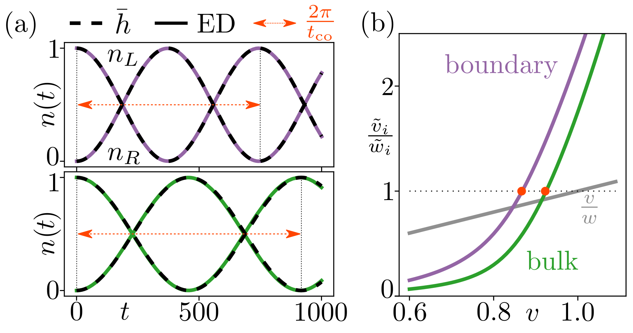
Figure 6: In (a): charge oscillations between aux. dots (initial localization left dot, ED,$U=200$ $N=20$, $\gamma=2$, $v=18$, $w=20$, OBC), with $l_{i}=\delta_{i,1}$,$r_{i}=\delta_{i,2}$ (upper,violet) and $l_{i}=\delta_{i,3}$,$r_{i}=\delta_{i,4}$ (lower,green). Analytical result (dashed) governed by Eq.(90). In (b): staggering for OBC inverting at the boundary close to topological transition $v=w$. Same parameters as in $(a)$.

We comment on the renormalization of the GFZ-Hamiltonian of Eq.(55) by the spin-spin correlation functions. In particular, we focus on the topological features of the underlying SSH model. We consider a finite-size SSH-Hubbard chain, where the non-interacting system shows zero-energy edge modes as a function of the staggered hopping ratio $v/w$. As described by to Eq.(55), the bare hoppings get renormalized significantly by the spin-correlation values. Since the SSH model at large U is effectively a spin chain, its ground state will obey Affleck-Kennedy-Lieb-Tasaki (AKLT) physics [70], with the formation of spin-singlet dimers in correspondence with the stronger bonds. As a consequence, the original imbalance between the non-interacting $v$ and $w$ is further amplified. In Fig.(6)(b) we show the behavior of the renormalized ratio $\frac{\tilde{v}}{\tilde{w}}$ as a function of $v$, for $w=20$ and $U=200$. The grey line shows the behavior of the bare hopping ratio. It is immediate to notice how the renormalized ratio varies much more heavily, passing from strong suppression to strong enhancement. The purple and green curves in the plot refer to different positions along the finite SSH chain, respectively near the boundary and deep in the bulk. Finite-size effect entail a different renormalization in the two cases, and the topological transition, denoted by the red dots, happens at the boundary sites for a lower value of $v/w$ than in the bulk. In the region between the two red dots, the boundary sites are already in the trivial phase, while the bulk is topological. As a consequence, edge state reconstruction ensues [71], with the topological edge zero described in [33] shifting into the bulk.

Appendix F Minimal chain to resolve the spin renormalization

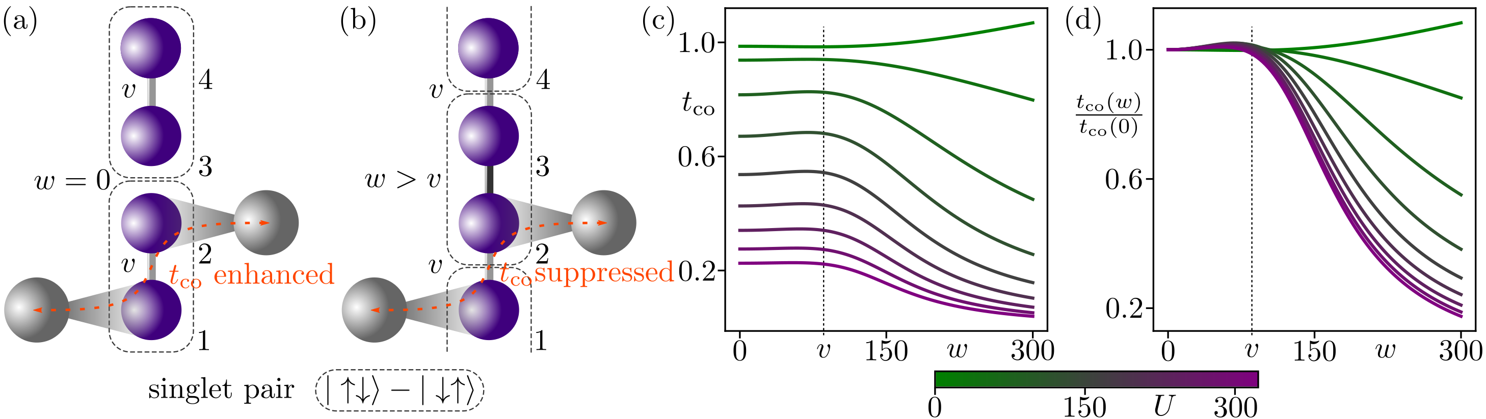
Figure 7: In (a) and (b): small chain of two coupled Hubbard dimers and lead dots at site 1 and 2 $l_{i}=\delta_{i,1}$,$r_{i}=\delta_{i,2}$. (a): Two uncoupled dimers with spin-singlet at bonds 1-2 and 3-4, probed $t_{\text{co}}$ at bond 1-2 is enhanced by the spin correlation $\langle\overrightarrow{S}_{1}\cdot\overrightarrow{S}_{2}\rangle$. (b): spin-singlet at bonds 2-3 and 1-4, probed $t_{\text{co}}$ at bond 1-2 is suppressed by the spin correlation $\langle\overrightarrow{S}_{1}\cdot\overrightarrow{S}_{2}\rangle$. In (c) and (d): expected (normalized) co-tunneling $t_{\text{co}}$ as function of $w$ and $U$ (ED, $N=12$, fixed $U=400$ on the lead dots, $v=100$, $l_{i}=\delta_{i,1}$,$r_{i}=\delta_{i,2}$), showing decreasing $t_{\text{co}}$ for increasing $w$ within the Mott regime (purple).

The minimal chain to resolve the spin renormalization consists of four quantum dots modeling the central Hubbard system. Thereby, two Hubbard dimers are coupled by the tunable tunneling $w$ (see Fig.7 (a) and (b)). Then, depending on $w$, we probe two regimes: first for $v>w$ (Fig.7 (a)), the system behaves as two uncoupled Hubbard dimers. In the strongly correlated limit its groundstate is then effectively described by two spin-singlets along the outer bonds. Secondly, for $w>v$ (Fig.7 (b)), the situation is quite different, now it forms a spin-singlet at the central bond and between the spins a the edges. As a result, the spin correlation along the probed, lower bond $\langle\overrightarrow{S}_{1}\cdot\overrightarrow{S}_{2}\rangle$ is maximal in the first case ($v>w$) since both the spins at site 1 and site 2 are maximally entangled. Whereas in the second case ($v<w$), $\langle\overrightarrow{S}_{1}\cdot\overrightarrow{S}_{2}\rangle$ is decreased, as both the spins at site 1 and site 2 are essentially uncorrelated. Via Eq.(55), the correlation function significantly alters the hopping in the GFZ Hamiltonian $H^{z}$ at the probed bond and eventually the measured co-tunneling amplitude $t_{\text{co}}$. In Fig.7 (c) we show the expected co-tunneling amplitude as function of the central tunneling $w$ for various correlation strengths $U$. When the system is deep in the Mott regime (large $U$, dark purple), the tunneling amplitude remains nearly constant for $v<w$ but decreases for $w>v$. Remarkably, this effect persists even outside the optimal Mott regime and only vanishes beyond the Mott transition. Where in the weakly interacting regime (green), the trend is slightly inverted: the co-tunneling amplitude increases with larger $w$, ruling out alternative explanations for the tunneling suppression observed in the Mott regime. In Fig.7 (d) we normalized each curve by the initial value at $w=0$, to highlight this effect . For an experimental verification, it is sufficient to observe the decreasing co-tunneling amplitude with increasing $w$, providing a clear qualitative signature of the effect. Precise fine-tuning or knowledge of the tunnelings $v,w$, correlation strength $U$ or the lead-system coupling $C$ is not necessary.

References

- Datta [1995] S. Datta, Electronic Transport in Mesoscopic Systems, Cambridge Studies in Semiconductor Physics and Microelectronic Engineering (Cambridge University Press, 1995).
- Ryndyk et al. [2009] D. A. Ryndyk, R. Gutiérrez, B. Song, and G. Cuniberti, Green Function Techniques in the Treatment of Quantum Transport at the Molecular Scale, in Energy Transfer Dynamics in Biomaterial Systems, edited by I. Burghardt, V. May, D. A. Micha, and E. R. Bittner (Springer Berlin Heidelberg, Berlin, Heidelberg, 2009) pp. 213–335.
- Ihn [2009] T. Ihn, Semiconductor Nanostructures: Quantum states and electronic transport (Oxford University Press, 2009).
- van der Wiel et al. [2002] W. G. van der Wiel, S. De Franceschi, J. M. Elzerman, T. Fujisawa, S. Tarucha, and L. P. Kouwenhoven, Electron transport through double quantum dots, Rev. Mod. Phys. 75, 1 (2002).
- Anisimov and Izyumov [2010] V. Anisimov and Y. Izyumov, Electronic Structure of Strongly Correlated Materials (Springer Berlin, Heidelberg, 2010) p. 291.
- Avella and Mancini [2011] A. Avella and F. Mancini, Strongly Correlated Systems: Theoretical Methods (Springer Berlin, Heidelberg, 2011) p. 464.
- Qin et al. [2022] M. Qin, T. Schäfer, S. Andergassen, P. Corboz, and E. Gull, The Hubbard Model: A Computational Perspective, Annual Review of Condensed Matter Physics 13, 275–302 (2022).
- Arovas et al. [2022] D. P. Arovas, E. Berg, S. A. Kivelson, and S. Raghu, The hubbard model, Annual Review of Condensed Matter Physics 13, 239–274 (2022).
- Barthelemy and Vandersypen [2013] P. Barthelemy and L. M. K. Vandersypen, Quantum Dot Systems: a versatile platform for quantum simulations, Annalen der Physik 525, 808 (2013).
- Nichol [2022] J. M. Nichol, Quantum-Dot Spin Chains, in Entanglement in Spin Chains: From Theory to Quantum Technology Applications, edited by A. Bayat, S. Bose, and H. Johannesson (Springer International Publishing, Cham, 2022) pp. 505–538.
- Hensgens et al. [2017] T. Hensgens, T. Fujita, L. Janssen, X. Li, C. J. Van Diepen, C. Reichl, W. Wegscheider, S. Das Sarma, and L. M. K. Vandersypen, Quantum simulation of a Fermi–Hubbard model using a semiconductor quantum dot array, Nature 548, 70–73 (2017).
- Qiao et al. [2020] H. Qiao, Y. P. Kandel, S. K. Manikandan, A. N. Jordan, S. Fallahi, G. C. Gardner, M. J. Manfra, and J. M. Nichol, Conditional teleportation of quantum-dot spin states, Nature Communications 11 (2020).
- Pustilnik and Glazman [2004] M. Pustilnik and L. Glazman, Kondo effect in quantum dots, Journal of Physics: Condensed Matter 16, R513–R537 (2004).
- Wang et al. [2023] Q. Wang, S. L. D. ten Haaf, I. Kulesh, D. Xiao, C. Thomas, M. J. Manfra, and S. Goswami, Triplet correlations in Cooper pair splitters realized in a two-dimensional electron gas, Nature Communications 14 (2023).
- Banerjee et al. [2018] M. Banerjee, M. Heiblum, V. Umansky, D. E. Feldman, Y. Oreg, and A. Stern, Observation of half-integer thermal hall conductance, Nature 559, 205–210 (2018).
- Kasahara et al. [2018] Y. Kasahara, T. Ohnishi, Y. Mizukami, O. Tanaka, S. Ma, K. Sugii, N. Kurita, H. Tanaka, J. Nasu, Y. Motome, T. Shibauchi, and Y. Matsuda, Majorana quantization and half-integer thermal quantum Hall effect in a Kitaev spin liquid, Nature 559, 227–231 (2018).
- Bartolomei et al. [2020] H. Bartolomei, M. Kumar, R. Bisognin, A. Marguerite, J.-M. Berroir, E. Bocquillon, B. Plaçais, A. Cavanna, Q. Dong, U. Gennser, Y. Jin, and G. Fève, Fractional statistics in anyon collisions, Science 368, 173–177 (2020).
- Nakamura et al. [2020] J. Nakamura, S. Liang, G. C. Gardner, and M. J. Manfra, Direct observation of anyonic braiding statistics, Nature Physics 16, 931–936 (2020).
- Dzyaloshinskii [2003] I. Dzyaloshinskii, Some consequences of the Luttinger theorem: The Luttinger surfaces in non-Fermi liquids and Mott insulators, Phys. Rev. B 68, 085113 (2003).
- Stanescu et al. [2007] T. D. Stanescu, P. Phillips, and T.-P. Choy, Theory of the Luttinger surface in doped Mott insulators, Phys. Rev. B 75, 104503 (2007).
- Sakai et al. [2009] S. Sakai, Y. Motome, and M. Imada, Evolution of electronic structure of doped Mott insulators: Reconstruction of poles and zeros of Green’s function, Phys. Rev. Lett. 102, 056404 (2009).
- Sakai et al. [2010] S. Sakai, Y. Motome, and M. Imada, Doped high- cuprate superconductors elucidated in the light of zeros and poles of the electronic Green’s function, Phys. Rev. B 82, 134505 (2010).
- Dave et al. [2013] K. B. Dave, P. W. Phillips, and C. L. Kane, Absence of Luttinger’s theorem due to zeros in the single-particle Green function, Phys. Rev. Lett. 110, 090403 (2013).
- Rosch [2007] A. Rosch, Breakdown of luttinger’s theorem in two-orbital mott insulators, Eur. Phys. J. B 59, 495–502 (2007).
- Gurarie [2011] V. Gurarie, Single-particle Green’s functions and interacting topological insulators, Phys. Rev. B 83, 085426 (2011).
- Essin and Gurarie [2011] A. M. Essin and V. Gurarie, Bulk-boundary correspondence of topological insulators from their respective green’s functions, Phys. Rev. B 84, 125132 (2011).
- Bollmann et al. [2024] S. Bollmann, C. Setty, U. F. P. Seifert, and E. J. König, Topological Green’s function zeros in an exactly solved model and beyond, Phys. Rev. Lett. 133, 136504 (2024).
- Zhao et al. [2023] J. Zhao, P. Mai, B. Bradlyn, and P. Phillips, Failure of topological invariants in strongly correlated matter, Phys. Rev. Lett. 131, 106601 (2023).
- Setty et al. [2024] C. Setty, F. Xie, S. Sur, L. Chen, M. G. Vergniory, and Q. Si, Electronic properties, correlated topology, and Green’s function zeros, Phys. Rev. Res. 6, 033235 (2024).
- Peralta Gavensky et al. [2023] L. Peralta Gavensky, S. Sachdev, and N. Goldman, Connecting the many-body Chern number to Luttinger’s theorem through Středa’s formula, Phys. Rev. Lett. 131, 236601 (2023).
- Pasqua et al. [2024] I. Pasqua, A. Blason, and M. Fabrizio, Exciton condensation driven by bound states of Green’s function zeros, Phys. Rev. B 110, 125144 (2024).
- Blason and Fabrizio [2023] A. Blason and M. Fabrizio, Unified role of Green’s function poles and zeros in correlated topological insulators, Phys. Rev. B 108, 125115 (2023).
- Wagner et al. [2023] N. Wagner, L. Crippa, A. Amaricci, P. Hansmann, M. Klett, E. J. König, T. Schäfer, D. D. Sante, J. Cano, A. J. Millis, A. Georges, and G. Sangiovanni, Mott insulators with boundary zeros, Nature Communications 14 (2023).
- Wagner et al. [2024] N. Wagner, D. Guerci, A. J. Millis, and G. Sangiovanni, Edge zeros and boundary spinons in topological Mott insulators, Phys. Rev. Lett. 133, 126504 (2024).
- Schleser et al. [2005] R. Schleser, T. Ihn, E. Ruh, K. Ensslin, M. Tews, D. Pfannkuche, D. C. Driscoll, and A. C. Gossard, Cotunneling-mediated transport through excited states in the Coulomb-blockade regime, Phys. Rev. Lett. 94, 206805 (2005).
- Braakman et al. [2013] F. R. Braakman, P. Barthelemy, C. Reichl, W. Wegscheider, and L. M. K. Vandersypen, Long-distance coherent coupling in a quantum dot array, Nature Nanotechnology 8, 432–437 (2013).
- Sánchez et al. [2014] R. Sánchez, G. Granger, L. Gaudreau, A. Kam, M. Pioro-Ladrière, S. A. Studenikin, P. Zawadzki, A. S. Sachrajda, and G. Platero, Long-range spin transfer in triple quantum dots, Phys. Rev. Lett. 112, 176803 (2014).
- Bordin et al. [2024] A. Bordin, X. Li, D. van Driel, J. C. Wolff, Q. Wang, S. L. D. ten Haaf, G. Wang, N. van Loo, L. P. Kouwenhoven, and T. Dvir, Crossed Andreev reflection and elastic cotunneling in three quantum dots coupled by superconductors, Phys. Rev. Lett. 132, 056602 (2024).
- Ranni et al. [2021] A. Ranni, F. Brange, E. T. Mannila, C. Flindt, and V. F. Maisi, Real-time observation of Cooper pair splitting showing strong non-local correlations, Nature Communications 12 (2021).
- Schindele et al. [2014] J. Schindele, A. Baumgartner, R. Maurand, M. Weiss, and C. Schönenberger, Nonlocal spectroscopy of Andreev bound states, Phys. Rev. B 89, 045422 (2014).
- Liu et al. [2022] C.-X. Liu, G. Wang, T. Dvir, and M. Wimmer, Tunable superconducting coupling of quantum dots via Andreev bound states in semiconductor-superconductor nanowires, Physical Review Letters 129 (2022).
- Mahan [1990] G. D. Mahan, Green’s functions at finite temperatures, in Many-Particle Physics (Springer US, Boston, MA, 1990) pp. 133–238.
- Bruus and Flensberg [2004] H. Bruus and K. Flensberg, Green’s functions, in Many–Body Quantum Theory in Condensed Matter Physics: An Introduction (Oxford University Press, 2004) p. 120–138.
- Fabrizio [2022] M. Fabrizio, Emergent quasiparticles at Luttinger surfaces, Nature Communications 13, 1561 (2022).
- Sakurai and Napolitano [2020] J. J. Sakurai and J. Napolitano, Approximation methods, in Modern Quantum Mechanics (Cambridge University Press, 2020) p. 288–370.
- Note [1] Due to expansions of terms, our approximation breaks down at large energies .
- Lehmann [2024] C. Lehmann, Supplemental Material (Appendix) (2025).
- Note [2] That is the correct groundstate towards the unperturbed limit and follows from degenerated perturbation theory.
- Note [3] The correlation value is evaluated in the limit towards, not at, the atomic limit, making it generally non-trivial.
- Anderson [1963] P. W. Anderson, Theory of magnetic exchange interactions: Exchange in insulators and semiconductors, in Solid State Physics, Solid State Physics, Vol. 14, edited by F. Seitz and D. Turnbull (Academic Press, 1963) pp. 99–214.
- Koch [2017] E. Koch, ed., Exchange Mechanisms (Autumn School on Correlated Electrons: The Physics of Correlated Insulators, Metals, and Superconductors, Jülich (Germany), 26 Sep 2017 - 26 Sep 2017, 2017).
- Pavarini et al. [2015] E. Pavarini, E. Koch, and P. Coleman, eds., Many-Body Physics: From Kondo to Hubbard, Schriften des Forschungszentrums Jülich. Reihe modeling and simulation, Vol. 5, Autumn School on Correlated Electrons, Jülich (Germany), 21 Sep 2015 - 25 Sep 2015 (Forschungszentrum Jülich GmbH Zentralbibliothek, Verlag, Jülich, 2015).
- Schrieffer and Wolff [1966] J. R. Schrieffer and P. A. Wolff, Relation between the Anderson and Kondo Hamiltonians, Phys. Rev. 149, 491 (1966).
- Bravyi et al. [2011] S. Bravyi, D. P. DiVincenzo, and D. Loss, Schrieffer–Wolff Transformation for Quantum Many-Body Systems, Annals of Physics 326, 2793–2826 (2011).
- Bir and Pikus [1974] G. Bir and G. Pikus, Irreducible representations and classification of terms, normal modes, perturbation theory, in Symmetry and Strain-induced Effects in Semiconductors, A Halsted Press book (Wiley, 1974) pp. 125–140.
- DiCarlo et al. [2004] L. DiCarlo, H. J. Lynch, A. C. Johnson, L. I. Childress, K. Crockett, C. M. Marcus, M. P. Hanson, and A. C. Gossard, Differential charge sensing and charge delocalization in a tunable double quantum dot, Phys. Rev. Lett. 92, 226801 (2004).
- Gaudreau et al. [2006] L. Gaudreau, S. A. Studenikin, A. S. Sachrajda, P. Zawadzki, A. Kam, J. Lapointe, M. Korkusinski, and P. Hawrylak, Stability diagram of a few-electron triple dot, Phys. Rev. Lett. 97, 036807 (2006).
- Wang et al. [2011] X. Wang, S. Yang, and S. Das Sarma, Quantum theory of the charge-stability diagram of semiconductor double-quantum-dot systems, Phys. Rev. B 84, 115301 (2011).
- Foulk and Das Sarma [2024] N. L. Foulk and S. Das Sarma, Theory of charge stability diagrams in coupled quantum dot qubits, Phys. Rev. B 110, 205428 (2024).
- Schleser et al. [2004] R. Schleser, E. Ruh, T. Ihn, K. Ensslin, D. C. Driscoll, and A. C. Gossard, Time-resolved detection of individual electrons in a quantum dot, Applied Physics Letters 85, 2005 (2004).
- Gustavsson et al. [2008] S. Gustavsson, R. Leturcq, B. Simovič, R. Schleser, T. Ihn, P. Studerus, K. Ensslin, D. C. Driscoll, and A. C. Gossard, Counting statistics of single electron transport in a semiconductor quantum dot, in Advances in Solid State Physics (Springer Berlin Heidelberg, Berlin, Heidelberg, 2008) pp. 31–43.
- Gustavsson et al. [2009] S. Gustavsson, R. Leturcq, M. Studer, I. Shorubalko, T. Ihn, K. Ensslin, D. Driscoll, and A. Gossard, Electron counting in quantum dots, Surface Science Reports 64, 191–232 (2009).
- Su et al. [1980] W. P. Su, J. R. Schrieffer, and A. J. Heeger, Soliton excitations in polyacetylene, Phys. Rev. B 22, 2099 (1980).
- Schollwöck [2005] U. Schollwöck, The density-matrix renormalization group, Reviews of Modern Physics 77, 259–315 (2005).
- Schollwöck [2011] U. Schollwöck, The density-matrix renormalization group in the age of matrix product states, Annals of Physics 326, 96–192 (2011).
- Yang and White [2020] M. Yang and S. R. White, Time-dependent variational principle with ancillary Krylov subspace, Phys. Rev. B 102, 094315 (2020).
- Paeckel et al. [2019] S. Paeckel, T. Köhler, A. Swoboda, S. R. Manmana, U. Schollwöck, and C. Hubig, Time-evolution methods for matrix-product states, Annals of Physics 411, 167998 (2019).
- Goto and Danshita [2019] S. Goto and I. Danshita, Performance of the time-dependent variational principle for matrix product states in the long-time evolution of a pure state, Phys. Rev. B 99, 054307 (2019).
- García Ripoll [2022] J. J. García Ripoll, Hamiltonian diagonalizations, in Quantum Information and Quantum Optics with Superconducting Circuits (Cambridge University Press, 2022) p. 270–276.
- Affleck et al. [1987] I. Affleck, T. Kennedy, E. H. Lieb, and H. Tasaki, Rigorous results on valence-bond ground states in antiferromagnets, Phys. Rev. Lett. 59, 799 (1987).
- Amaricci et al. [2017] A. Amaricci, L. Privitera, F. Petocchi, M. Capone, G. Sangiovanni, and B. Trauzettel, Edge state reconstruction from strong correlations in quantum spin Hall insulators, Phys. Rev. B 95, 205120 (2017).