Detecting Supernova Axions with IAXO

Abstract

We investigate the potential of IAXO and its intermediate version, BabyIAXO, to detect axions produced in core-collapse supernovae (SNe). Our study demonstrates that these experiments have realistic chances of identifying SN axions, offering crucial insights into both axion physics and SN dynamics. IAXO’s sensitivity to SN axions allows for the exploration of regions of the axion parameter space inaccessible through solar observations. In addition, in the event of a nearby SN, $d\sim\mathcal{O}(100)$ pc, and sufficiently large axion couplings, $g_{a\gamma}\gtrsim 10^{-11}\,{\rm GeV^{-1}}$, IAXO could have a chance to significantly advance our understanding of axion production in nuclear matter and provide valuable information about the physics of SNe, such as pion abundance, the equation of state, and other nuclear processes occurring in extreme environments.

March 5, 2025

1 Introduction

Axions [1, 2] are theoretically well-motivated pseudo-scalar particles, predicted by several extensions of the Standard Model. They are a robust prediction of the Peccei-Quinn (PQ) mechanism [3, 4] of the strong CP problem, which remains one of the great challenges in particle physics. Moreover, they are attractive dark matter (DM) candidates [5, 6, 7]. A quite extensive program is in place, worldwide, to detect these elusive particles. One of the most ambitious proposals is the International Axion Observatory (IAXO) [8], a new generation axion helioscope, which provides the sensitivity needed to probe a large section of the axion parameter space for a wide mass range. As a first step, the collaboration is building an intermediate-scale version, called BabyIAXO, which will function as a technological prototype for IAXO, as well as an independent physics experiment, with considerable discovery potential [9].

The size of the IAXO and BabyIAXO magnets provides a large conversion volume which, combined with a novel tracking system might permit the detection of an axion flux from a nearby supernova (SN), as originally proposed in Ref. [10, 11]. Though the closest SN candidates are at $\mathcal{O}(100)$ pc from us, the very large temperature and density in the core of the exploding star could generate an axion flux large enough to be detected by a next generation helioscope. Specifically, for a sufficiently near candidate, the axion flux on Earth (in ${\rm cm^{-2}\,s^{-1}}$) might be (even significantly) larger than the expected solar axion flux. The main difficulty, however, is that the SN axion flux drops rapidly after a few seconds, demanding readiness and a prompt intervention in case of such an event. Therefore, the helioscope as SN-scope concept should rely on an efficient alert system for coming SN events. The ability to anticipate a supernova event far enough in advance to prepare for observations is a topic of significant interest in current research. A methodology for a pre-supernova alert has been already implemented in KamLAND [12], and SNEWS 2.0 intends to develop and provide a pre-SN alert to inform of the coming CC event (see Sec. 4 of Ref. [13]). This capability practically relies on the detection of neutrinos emitted during the late evolutionary stages of a supergiant, particularly during the silicon-burning phase, which directly precedes the explosion (see Sec. 3 for more details).

The fast response time implemented in the IAXO and BabyIAXO helioscopes facilitates the implementation of IAXO as a SN-scope. In contrast to helioscope searches, where the expected axion signature is X-rays in the keV regime, the different SN production mechanisms lead to axion energies in the $10-250~\mathrm{MeV}$ energy range. Therefore, the detection of SN axions relies on the development of a highly efficient gamma-ray detector in addition to the X-ray detector. In particular, the gamma-ray detector should provide topological information to distinguish the signature of high energy axions from background events.

Given the current technology capabilities, the detection of axions from a nearby SN event is a realistic possibility and the construction of a dedicated MeV detector for the next generation of axion helioscopes is highly motivated. First, a sensitivity to SN axions would allow us to explore regions of the axion parameter space not accessible through solar observations. Second, such a detection could shed light on important aspects of the SN physics, not accessible through other experimental tests. SNe are very rare events with current estimates predicting a rate of $1.63\pm 0.46$ per century [14]. It is, therefore, imperative to ensure the highest level of preparedness for such an eventuality.

In this work, we focus on the theoretical and phenomenological aspects of the helioscope potential to detect axions from a nearby SN event. The discussion of the most appropriate MeV detector configuration for IAXO is presently ongoing and will be presented in a separate work.

This article is organized as follows. In Section 2 we summarize the different SN axion production mechanisms. Section 3 describes the different technical aspects for the implementation of IAXO and BabyIAXO for the detection of SN axions. In Section 4 the sensitivity prospects in different scenarios are presented. Finally, we conclude our discussion of IAXO as a SN-scope in Section 5. There follow Appendices with more technical details of our analysis.

2 Supernova axion production

Core-collapse SNe are among the most powerful astrophysical factories for the production of feebly-interacting particles. Indeed, the series of catastrophic events occurring during the onset of the gravitational collapse induces extreme conditions of temperature and density in the inner regions of the core (see Refs. [15, 16, 17] for some reviews). In particular, at the beginning of the cooling phase the core of an exploding SN is expected to be characterized by temperatures $T\sim 30-40\,\operatorname{MeV}$ and densities around the nuclear saturation $\rho\sim 10^{14}\,\operatorname{g}\,\operatorname{cm}^{-3}$. Under these conditions, the production of feebly-interacting particles, like axions and axion-like particles (ALPs), could be significantly enhanced. Therefore, a future galactic SN event may represent a once-in-a-lifetime opportunity to probe axion physics.

If axions are coupled to nuclear matter, the main production channels in the hot and dense SN core depend on their coupling to nucleons $g_{aN}$, with $N=n,\,p$ for neutrons and protons respectively [18, 19, 20]. The first considered channel for axion emission from the SN nuclear medium is $NN$ bremsstrahlung $N+N\rightarrow N+N+a$ [21, 22, 23, 24, 25]. As depicted in the left panel of Fig. 1, in this process an axion is produced as a consequence of strong interactions between two nucleons in the medium. The state-of-the-art calculation for the bremsstrahlung emission rate has been performed in Ref. [26] and accounts for corrections beyond the usual one-pion exchange (OPE) approximation for the nuclear interaction potential. In particular, a non-vanishing mass for the exchanged pion [27], the contribution from the two-pion exchange [28], effective in-medium nucleon masses and multiple nucleon scattering effects [29, 30] have to be taken into account to obtain a reliable estimation of the bremsstrahlung emissivity. Finally, Ref. [31] has discussed the impact of finite-density effects over ALP-nucleon couplings in dense environments. Furthermore, the right panel of Fig. 1 displays a schematic representation of pionic Compton-like processes $\pi+N\rightarrow a+N$, in which a pion is converted into an axion after the scattering onto a non-relativistic nucleon. Since in the SN nuclear medium the fraction of thermal pions $Y_{\pi}$ was expected to be extremely small $Y_{\pi}\sim\mathcal{O}(10^{-4})$ [32], the contribution from pion conversions has been overlooked for a long time. Nevertheless, the authors of Ref. [33] pointed out that strong interactions can magnify the abundance of negatively-charged pions. Thus, the pion conversion emission rate has been re-estimated in Ref. [34], realizing that, under the assumption of Ref. [33], it could be comparable and even dominant over the bremsstrahlung contribution. Moreover, it has been recently shown that the contribution from the contact interaction term [35] and the $\Delta(1232)$ resonance [36] can significantly enhance axion emissivity via pion conversion. We address the reader to Refs. [18, 37] for the complete expressions of both $NN$ bremsstrahlung and pion conversion emission rates.

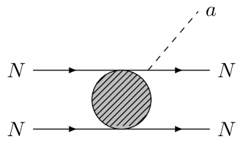
Figure 1: Schematic representation of the Feynman diagrams for the $NN$ bremsstrahlung (left panel) and the pionic Compton-like process (right panel).

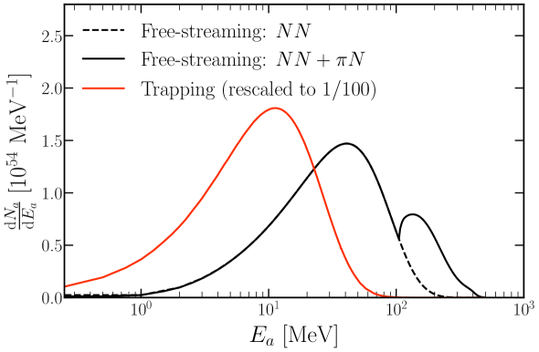
Figure 2: Time-integrated ALP emission spectrum from our benchmark SN model [38]. The continuous black line depicts the spectrum line-shape including both contributions from $NN$ bremsstrahlung ($NN$) and pion conversions ($\pi N$), while the dashed black line refers to the bremsstrahlung-only contribution in the free-streaming regime. The corresponding spectrum for the trapping regime is depicted as a continuous red line. Note that we rescaled the trapping curve by a factor of 1/100 for the visualization. Here the ALP-neutron coupling is fixed at $g_{an}=0$, while the ALP-proton coupling is set at $g_{ap}=5\times 10^{-10}$ free streaming scenario and at $g_{ap}=3\times 10^{-6}$ in the trapping case.

If axions are weakly coupled to nuclear matter, ${g_{aN}\lesssim 10^{-8}}$, they are in the free-streaming regime, in which they can leave the star without being reabsorbed by the nuclear medium in the SN core. Therefore, they can act as an additional energy-loss channel during the SN cooling phase, contributing to the shortening of the neutrino burst duration [39]. In particular, consistency with observations of the neutrino burst from SN 1987A requires ${g_{ap}\lesssim 5\times 10^{-10}}$ [19]. On the other hand, for sufficiently large couplings $g_{aN}\gtrsim 10^{-8}$, the SN core becomes “optically thick” for the produced axions, so that they can be also reabsorbed inside the core by means of the inverse processes $N+N+a\rightarrow N+N$ and $a+N\rightarrow\pi+N$ [19]. In this regime, dubbed trapping regime, axions are not able to escape the inner regions of the core and their emission can be approximately described as a blackbody radiation from a last-scattering surface [41], in close analogy with the case of neutrinos. We highlight that a complete treatment of the trapping regime would require the self-consistent addition of axions in SN simulations, since they could significantly impact the SN evolution. Relying just on the SN cooling argument, the range $5\times 10^{-10}\lesssim g_{ap}\lesssim 3\times 10^{-6}$ is excluded. However, larger values of the coupling can be constrained by the non observation of axion-induced events in Kamiokande-II during SN 1987A [42, 19]. Nevertheless, despite these constraints, even the trapped region remains a subject of interest for axion experiments [17].

In the following, we adopt as benchmark SN model the 1D spherical-symmetric GARCHING group’s SN model SFHo-s18.8 provided in Ref. [38], used also in previous studies about SN axions (see, e.g. Refs. [43, 44, 45, 18, 19, 46, 20]). The simulation, based on the neutrino-hydrodynamics code PROMETHEUS-VERTEX [47], is launched from a stellar progenitor with mass $18.8~M_{\odot}$ [48] and leads to a neutron star (NS) with baryonic mass $1.35~M_{\odot}$, a typical value expected for a SN explosion event [15]. More details on the employed SN model are provided in Appendix A. The presence of pions in the SN core has been taken into account by following the procedure illustrated in Ref. [49], including the pion-nucleon interaction as described in Ref. [33]. Figure 2 shows the axion emission spectrum integrated over $10\,\operatorname{s}$ in both the free-streaming (black lines) and trapping regimes (red line) for our benchmark SN model. In the free-streaming regime, the spectrum is characterized by a bimodal shape, since the emission peak associated with the $NN$ bremsstrahlung is located at axion energies $E_{a}\sim 50\,\operatorname{MeV}$, while the pion conversion contribution peaks at $E_{a}\sim 200\,\operatorname{MeV}$ [18, 19]. This is related to the different nature of the two processes. In particular, the bremsstrahlung behaves as a quasi-thermal process, so that the average energy of the emitted ALP can be estimated as $E_{a}\simeq\frac{3}{2}T$  [46]. On the other hand, the pion conversion is highly non-thermal and the average ALP energy is given by $E_{a}\simeq\,m_{\pi}+\frac{3}{2}T$, where $m_{\pi}\simeq 135\,\operatorname{MeV}$ is the pion mass.

By summing the contributions from both nuclear processes, the axion emission spectrum is expected to have the form [18, 19]

$$\frac{dN_{a}}{dE_{a}}=A\,g_{aN}^{2}\left[F_{NN}(E_{a})+\delta\,F_{\pi N}(E_{a})\right]\,.$$ (2.1)

Here, $A$ is a normalization factor, with the dependence on the axion coupling constant factorized for convenience. The functions $F_{NN}$ and $F_{\pi N}$ encode the spectral shape of bremsstrahlung and pionic processes, respectively. These functions, as well as $A$, depend on the specific SN model, in particular on the equation of state employed and on the specific plasma conditions in the SN nuclear medium (simple fitting expressions for axion spectra, considering a range of supernova simulations, can be found in Ref. [46]). Finally, $\delta$ is a free parameter that quantifies the relative contributions of $F_{NN}$ and $F_{\pi N}$ with respect to the benchmark model (corresponding to $\delta=1$ and shown in Fig. 2). Therefore, $\delta$ serves as an indicator of the pion abundance in the proto-neutron star (PNS), normalized so that $\delta=1$ corresponds to a pion-to-nucleon fraction $Y_{\pi}\sim\mathcal{O}(1)\%$ in the inner core regions (see Appendix A for further details).

In the trapping regime, axions are emitted from outer regions of the SN core at ${R\sim 15-20\,\operatorname{km}}$ where the temperature is in the range of few MeV. Under these conditions, the pion conversion peak is completely suppressed, while the average energy of ALPs produced by $NN$ bremsstrahlung processes is shifted towards lower values $E_{a}\sim 10\,\operatorname{MeV}$ [19].

3 Direct detection of SN axions in IAXO

The novel tracking system for new generation axion helioscopes offers the possibility to point at a specific target within a few minutes [9]. We plan to take advantage of this system to detect SN axions with IAXO, by orienting it toward the SN. In this section we present a detailed and realistic analysis for the detection possibilities with IAXO.

The list of nearby SN candidates is presented in Table  1. A corresponding Mollweide projection of the position of the listed candidates in the galactic plane is subsequently presented in Figure 3. Examples of the error expected in the directional determination for three selected candidates are shown in Tab. 2. The data is available in Ref. [50], though we have integrated it with the more recent red supergiant catalog presented in Ref. [51] and crosschecked with the simbad database [52]. We limit our list to $d<300$ pc as the axion flux from more distant stars would be too small to be detected with IAXO.

$N$	Catalog Name	Common Name	Distance [kpc]	RA [J2000]	Dec [J2000]
1	HD 116658	Spica/$\alpha$ Virginis	0.077 $\pm$ 0.004	13:25:11.58	-11:09:40.8
2	HD 149757	$\zeta$ Ophiuchi	0.112 $\pm$ 0.002	16:37:09.53	-10:34:01.5
3	HD 129056	$\alpha$ Lupi	0.143 $\pm$ 0.003	14:41:55.79	-47:23:17.52
4	HD 78647	$\lambda$ Velorum	0.167 $\pm$ 0.003	09:02:06.85	-43:31:17.72
5	HD 148478	Antares/$\alpha$ Scorpii	0.169 $\pm$ 0.003	16:29:24.46	-26:25:55.2
6	HD 206778	$\epsilon$ Pegasi	0.211 $\pm$ 0.006	21:44:11.16	+09:52:30.0
7	HD 157244	$\beta$ Arae	$0.219\pm 0.010$	17:25:17.99	-55:31:47.57
8	HD 39801	Betelgeuse/$\alpha$ Orionis	0.222 $\pm$ 0.040	05:55:10.31	+07:24:25.4
9	HD 89388	q Car/V337 Car	0.230 $\pm$ 0.022	10:21:20.75	-61:48:29.2
10	HD 210745	$\zeta$ Cephei	0.256 $\pm$ 0.006	22:10:51.23	+58:12:04.4
11	HD 34085	Rigel/$\beta$ Orionis	0.264 $\pm$ 0.024	05:14:32.27	-08:12:05.9
12	HD 209005	$\zeta$ Cygni	0.278 $\pm$ 0.029	21:19:51.82	+30:13:49.2
13	HD 47839	S Monocerotis A	0.282 $\pm$ 0.040	06:40:58.66	+09:53:44.7
14	HD 47839	S Monocerotis B	0.282 $\pm$ 0.040	06:40:58.66	+09:53:44.7
15	HD 93070	q Car/V520 Car	0.294 $\pm$ 0.023	10:43:32.49	-60:06:29.0

Table 1: List of all SN candidates at distance $d\leq 300$ pc. The catalog name refers to the Henry Draper (HD) catalog number. Data from Refs. [50, 51] and the simbad database [52].

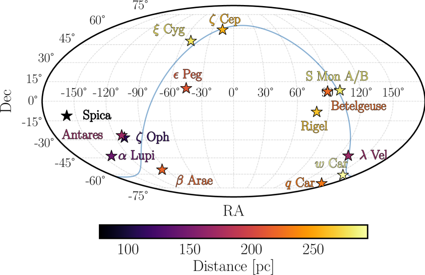
Figure 3: Mollweide projection of the SN candidates presented in Tab. 1. The Galactic plane, defined by latitude 0 in the Galactic coordinate system, is depicted as a continuous blue line across the sky. The color scheme encodes the distance of the stars from Earth in parsec.

It is evident that the detection of SN axions using IAXO and BabyIAXO relies heavily on our ability to predict core-collapse SN events with sufficient advance notice and angular precision to plan observations effectively. For this purpose, one has to rely on an early-alert system. Effectively, this is possible through the observation of pre-SN neutrinos, as the neutrino production rises rapidly during the last stages of nuclear burning [53]. Although the flux remains substantially lower—and at lower energies—than what is expected during the explosion itself, these neutrino fluxes are predicted to be observable in dedicated detectors minutes to days before the rise of the electromagnetic emission, providing the desired early alert (see, e.g., Ref. [53]). Dedicated analyses indicate, for example, that the combined analysis of KamLAND and Super-Kamiokande (SK) can detect the pre-SN neutrino flux from stars up to $\sim$ 500 pc, providing an early warning up to $\sim 12$ hours before the SN event [54]. Extracting directional information is more challenging. A detailed study of the potential to accurately detect the position of the source from pre-SN observations was presented in Ref. [50]. Information about the upcoming event, including positional data, is expected to be available hours before the event, a time more than sufficient to turn the IAXO telescope towards the star. The directional sensitivity of these events is relatively low, due to the weak forward-backward asymmetry of the inverse beta decay process used to detect the neutrino events. For current liquid scintillators, the low value of this asymmetry translates into a moderate angular resolution of around $60^{\circ}$ when 200 events are detected, which is realistic for a star like Betelgeuse. The use of a lithium-loaded liquid scintillator (LS-Li) would substantially increase the forward-backward asymmetry, pushing the angular resolution to about $15^{\circ}$ with the same number of events. Further improvements are possible with proposed future neutrino detectors, such as THEIA [55].

$N$	Time before Supernova	Angular Error (68.8% C.L.)	Candidates within Cone
5	$4\,\text{h}$	$16.44^{\circ}$	2
5	$1\,\text{h}$	$11.16^{\circ}$	1
5	$2\,\text{min}$	$8.54^{\circ}$	1
8	$4\,\text{h}$	$23.24^{\circ}$	4
8	$1\,\text{h}$	$15.47^{\circ}$	3
8	$2\,\text{min}$	$11.63^{\circ}$	1-2
13	$2\,\text{h}$	$48.26^{\circ}$	7
13	$1\,\text{h}$	$19.00^{\circ}$	2-3
13	$2\,\text{min}$	$9.84^{\circ}$	1

Table 2: Angular error and number of candidates within the error cone over time for three supernovae candidates assuming the usage of LS-Li detectors. All three candidates are visible more then 50% of the time for BabyIAXO. The candidates are identified by their index $N$ from Tab. 1. Data from Ref. [50].

Despite the moderate angular precision expected in the case of pre-SN neutrino events, the information provided by an early warning system may suffice to identify the SN candidate, given that the sample of possible close-by candidates is known (see Tab. 1), and that their relative angular distances are in most cases relatively large (cf. Tab. 5 in Appendix B).

An important consideration is the tracking range of IAXO, for which no definite configuration has been determined, aside from the requirement that the altitude angle, measured relative to the horizon, covers a symmetric range that extends at least from $-21.1^{\circ}$ to $+21.1^{\circ}$ [56, 9]. For reference, in our analysis we consider three realistic scenarios corresponding to altitude ranges of $\pm 20^{\circ}$, $\pm 25^{\circ}$, and $\pm 30^{\circ}$. In Fig. 4, we show the example of the daily variation of the altitude of three representative SN candidates, Spica, Antares and Betelgeuse, as seen from an observatory located at DESY (Hamburg, Germany), where (Baby)IAXO will be hosted.

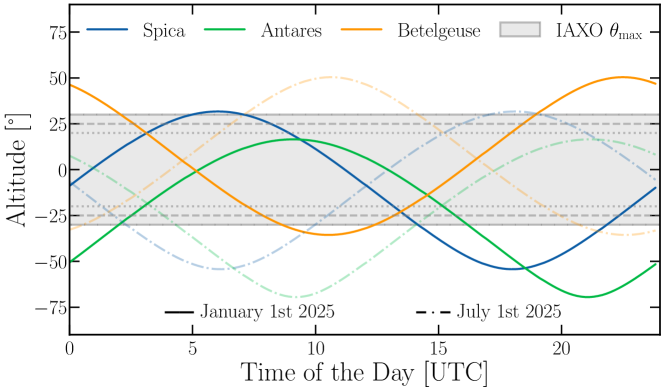
Figure 4: Daily variation of the altitude of three representative SN candidates, Spica, Antares and Betelgeuse, as observed from DESY on the first of January and on the first of July 2025. The gray area highlights the altitudes accessible by IAXO for the three cases $\theta_{\mathrm{max}}$ = 20° (dotted), 25° (dashed) and 30° (solid line) studied in this work, cf. Tab. 3.

The figure shows the altitude for two representative days (chosen without any specific reason) to highlight the annual modulation induced by the Earth rotation. It is evident that the limited tracking possibilities of the telescope prevent the observation of the star in some period of the day. We have calculated the percentage of the time during which each star in Tab. 1 is visible from DESY. The results are shown in Tab. 3, where the stars are identified via their index $N$ and common name, as defined in Tab. 1.

$N$	Common Name	Observable Time Fraction [%]
		$\theta_{\rm max}=20^{\circ}$	$\theta_{\rm max}=25^{\circ}$	$\theta_{\rm max}=30^{\circ}$
1	Spica/$\alpha$ Virginis	43	63	70
2	$\zeta$ Ophiuchi	42	59	71
3	$\alpha$ Lupi	28	36	43
4	$\lambda$ Velorum	33	40	46
5	Antares/$\alpha$ Scorpii	49	54	59
6	$\epsilon$ Pegasi	42	57	71
7	$\beta$ Arae	9	24	34
8	Betelgeuse/$\alpha$ Orionis	41	54	74
9	q Car/V337 Car	0	0	23
10	$\zeta$ Cephei	0	18	30
11	Rigel/$\beta$ Orionis	41	55	73
12	$\zeta$ Cygni	46	51	56
13	S Monocerotis A	42	57	71
14	S Monocerotis B	42	57	71
15	q Car/V520 Car	0	11	26

Table 3: Potential time fractions for observations of the stars listed in Tab. 1, identified by their index $N$ and common names.

4 Sensitivity prospects

Axions could be abundantly produced during a core-collapse SN event with energies of about 10–250 MeV, as shown in Fig. 2. The probability of axion to photon conversion inside an approximately uniform magnetic field $B$ with a length $L$ can be reduced to [57, 58]

$$P_{a\rightarrow\gamma}=\left(\frac{g_{a\gamma}BL}{2}\right)^{2}\left[\frac{\sin\left(\frac{qL}{2}\right)}{\frac{qL}{2}}\right]^{2},$$ (4.1)

where $g_{a\gamma}$ is the axion-to-photon coupling constant and $q$ is the momentum transfer between the axion and the photon. In the relativistic limit, in vacuum,

$$q=\frac{m_{a}^{2}}{2E_{a}},$$ (4.2)

where $m_{a}$ is the axion mass and $E_{a}$ the axion energy. Therefore, the number of expected signal counts $S_{\gamma}$ associated to the ALP emission during the SN cooling phase lasting $\sim 10\,\operatorname{s}$, is given by

$$S_{\gamma}=\frac{1}{4\pi D^{2}}\int_{E_{i}}^{E_{f}}\mathrm{d}E\,\frac{\mathrm{d}N_{a}}{\mathrm{d}E}\,P_{a\rightarrow\gamma}\,\epsilon\,A=g_{a\gamma}^{2}\,g_{aN}^{2}\int_{E_{i}}^{E_{f}}\mathrm{d}E\,\frac{\mathrm{d}n_{\gamma}}{\mathrm{d}E},$$ (4.3)

where ${\mathrm{d}N_{a}}/{\mathrm{d}E}$ is the emitted axion spectrum integrated over $\sim 10\,\operatorname{s}$, defined in Eq. (2.1); $D$ is the SN distance; $P_{a\rightarrow\gamma}$ is the conversion probability of the axion into a photon in a uniform magnetic field, presented in Eq. (4.1); $\epsilon$ is the detector efficiency and $A$ is the magnet bore area. The second identity of Eq. (4.3), together with Eq. (2.1), define the quantity $dn_{\gamma}/dE$, which parameterizes (though it is not exactly equal to) the number counts per energy. For future convenience, it is useful to split this function into the bremsstrahlung and pion parts:

$$n_{\gamma}=n_{\gamma}^{NN}+\delta\cdot n_{\gamma}^{\pi N}\,,$$ (4.4)

which follows our definition in Eq. (2.1). Under the assumption of zero detected counts and zero background expected counts, the exclusion limit at a 95% of C.L. is given by:

$$S_{\gamma}=g_{a\gamma}^{2}\,g_{aN}^{2}\int_{E_{i}}^{E_{f}}\mathrm{d}E\,\frac{\mathrm{d}n_{\gamma}}{\mathrm{d}E}\leq\operatorname{ln}(20)$$ (4.5)

Sensitivity prospects are shown in Fig. 5 and 6 for two different SN progenitor candidates, namely Spica ($\alpha$ Virginis) and Betelgeuse ($\alpha$ Orionis). These prospects have been computed in different helioscope scenarios: BabyIAXO, consisting of two magnetic bores, with a length $L=10$ m and an area $A=0.77$ m² as well as an average magnetic field $B=2$ T; IAXO, which will be equipped with 8 magnet bores with $L=20$ m and $A=2.3$ m², providing a magnetic field of strength $B=2.5$ T; and IAXO+, which represents an enhanced version of IAXO, with a magnetic field $B=3.5$ T, an area $A=3.9$ m² and magnet bores with $L=22$ m. These helioscope scenarios are described in Ref. [9] and summarized in Table 4. For the high-energy gamma detector we assume a conservative detection efficiency of $\epsilon=95\%$ and an energy threshold of 3 MeV.

	$B$ (T)	$L$ (m)	$A$ (m2)
BabyIAXO	2	10	0.77
IAXO	2.5	20	2.3
IAXO+	3.5	22	3.9

Table 4: Magnetic field strength $B$, length $L$, and cross sectional area $A$ for BabyIAXO, IAXO and IAXO+ [9].

In contrast to helioscope searches, where the sensitivity drops rapidly after 10 meV, the coherence region for SN axions is extended to above 1 eV. This allows for a wider range of the parameter space to be explored, including the theoretically most favoured axion models.

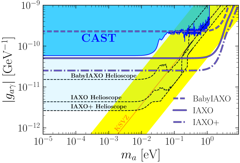
(a) $NN$: Betelgeuse

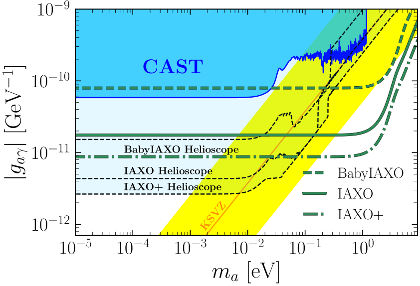
(b) $NN$: Spica

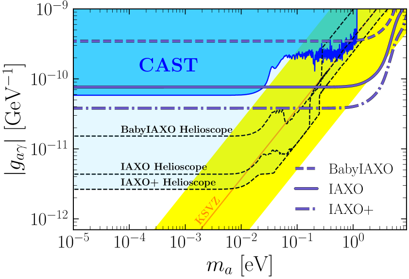
(c) $NN+\pi N$: Betelgeuse

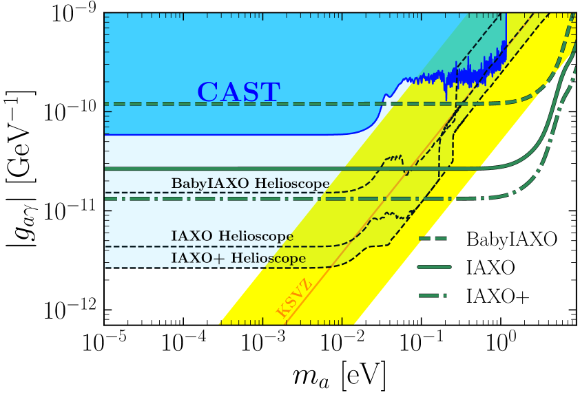
(d) $NN+\pi N$: Spica

Figure 5: Sensitivity prospects for BabyIAXO, IAXO and IAXO+ as SNScopes for Betelgeuse (violet, left panel) and Spica (green, right panel) in the ALP free streaming regime considering bremsstrahlung emission and both bremsstrahlung and pion conversion emission. In the upper panels, we set the ALP-nucleon coupling to ${g_{aN}=10^{-9}}$, while in the lower panels we set it to the maximum value allowed by the the SN cooling argument ${g_{aN}=5\times 10^{-10}}$. The black transparent regions show the sensivity prospects of IAXO, BabyIAXO and IAXO+ as helioscopes.

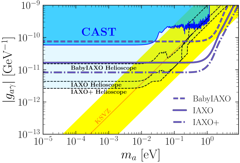
(a) Trapping: Betelgeuse

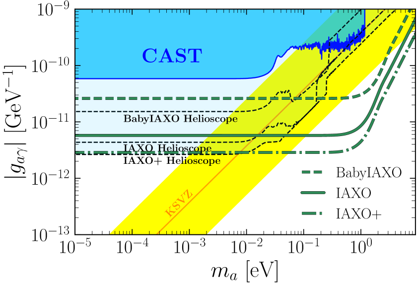
(b) Trapping: Spica

Figure 6: Sensivity prospects for BabyIAXO, IAXO and IAXO+ as SNScopes for Betelgeuse (violet, left panel) and Spica (green, right panel) in the trapping regime. Again, here we set the ALP-nucleon coupling to the minimum value allowed by the upper limit of SN cooling bound ${g_{aN}=3\times 10^{-6}}$ [19]. The blue transparent regions show the sensivity prospects of IAXO, BabyIAXO and IAXO+ as helioscopes.

In case of a positive SN axion signature, the energy spectrum of the detected counts will provide precious information about the axion production mechanisms during the core-collapse SN. Here we discuss the signal analysis for the free-streaming regime under the assumption of bremsstrahlung and pion conversion emission. At given value of the ALP-nucleon coupling $g_{aN}$, the number of axions emitted via pion conversion processes is highly dependent on the pion abundance in the supernova core, a factor which remains under investigation. In order to perform a model independent signal analysis, we employ a two-dimensional likelihood analysis in which the probability density function is given by the Poisson distribution. Thus, the likelihood function can be written as

$$L=\frac{1}{L_{0}}\prod_{i=1}^{n}e^{-\operatorname{s}_{i}}\frac{\operatorname{s}_{i}^{ni}}{n_{i}!},\qquad L_{0}=\prod_{i=1}^{n}e^{-n_{i}}\frac{n_{i}^{ni}}{n_{i}!},$$ (4.6)

where $L_{0}$ is the normalization factor, the index $i$ refers to the energy bin, $n_{i}$ is the number of counts measured in the $i$th bin and $\operatorname{s}_{i}$ is the expected number of signal counts in the $i$th bin,

$$\operatorname{s}_{i}=g_{a\gamma}^{2}\,g_{aN}^{2}\int_{E_{i}}^{E_{i}+\Delta E}\mathrm{d}E\,\frac{\mathrm{d}n_{\gamma}^{NN}}{\mathrm{d}E}\,+\,g_{a\gamma}^{2}\,g_{aN}^{2}\,\delta\,\int_{E_{i}}^{E_{i}+\Delta E}\frac{\mathrm{d}n_{\gamma}^{\pi N}}{\mathrm{d}E}\mathrm{d}E,$$ (4.7)

with the integral over the signal counts performed between $E_{i}$ and $E_{i}+\Delta E$, referring to the corresponding energy bin $i$ and assuming a bin size of $\Delta E$ =1 MeV.

Instead of using the natural likelihood, it is more convenient to work with the logarithm of the likelihood $\ln{L}$. According to Wilks’ theorem [59], if certain general conditions are satisfied, the minimum of $-2\ln{L}$ approaches a $\chi^{2}$ distribution

$$-\frac{\chi^{2}}{2}=\ln{L}=\sum_{i=1}^{n}n_{i}-\operatorname{s}_{i}+n_{i}\log{\frac{\operatorname{s}_{i}}{n_{i}}}.$$ (4.8)

The likelihood analysis is performed for a fixed axion mass in the coherence region ($m_{a}=0.01$ eV) while scanning over the $g_{a\gamma}^{2}\times g_{aN}^{2}$ and $\delta$ parameter space. The minimum of the $\chi^{2}$ distribution is extracted, in which the shift of one $\chi^{2}$ unit corresponds to one standard deviation ($\sigma$) in the parameter estimation. Fig. 7 and Fig. 8 show an illustrative example of the likelihood analysis results for 10 detected counts, using as input distribution the free streaming case of Fig. 2 with $\delta=1$ and a coupling constant of $g_{aN}=5\times 10^{-10}$. Being the best fit parameters close to their truth values, these results probe the physics potential of IAXO in reconstructing quantities relevant for SN axion emission, if a detection is achieved.

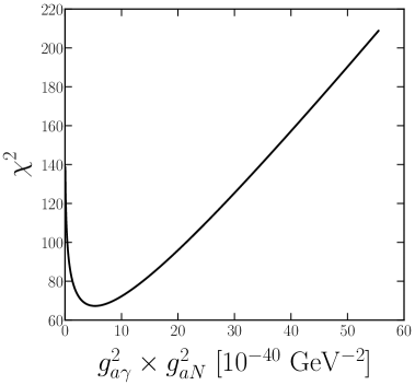
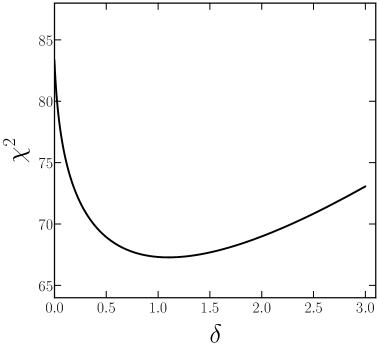
Figure 7: $\chi^{2}$ as a function the different likelihood analysis parameters: $g_{a\gamma}^{2}g_{aN}^{2}$ (left) and the fraction of pions $\delta$ (right).

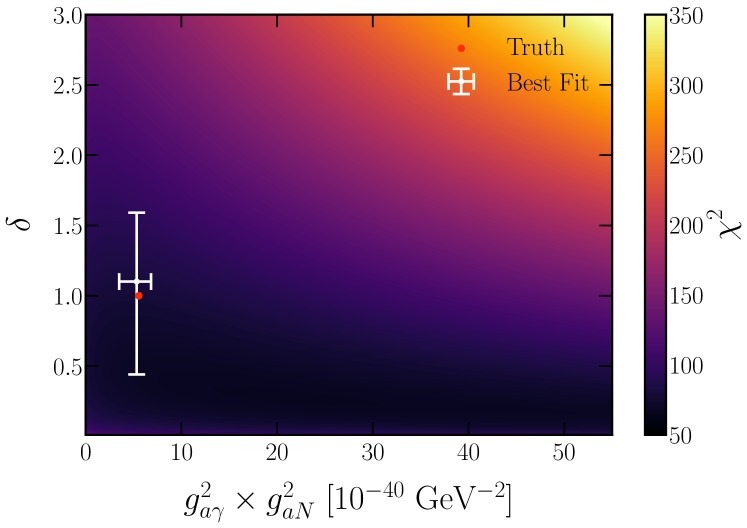
Figure 8: Likelihood analysis results in the $g_{a\gamma}^{2}g_{aN}^{2}$ and $\delta$ parameter space, in which the color palette shows the value of the $\chi^{2}$ distribution. The red dot represents the truth value of the SN axion model used as input for the calculations, while the white marker shows the minimum of the likelihood analysis in which the error bars correspond to one standard deviation ($\sigma$).

5 Discussion and Conclusions

In this work, we have presented an updated study of the SN axion flux expected from a nearby SN and the corresponding signal it would generate in a helioscope experiment. Our analysis includes axion production from pion-Compton processes, which had not been previously accounted for, despite potentially being the dominant production channel.

We have shown that if a nearby supernova (SN) occurs, IAXO—and, to a somewhat lesser extent, BabyIAXO—could have a realistic chance of detecting QCD axions in regions of parameter space that are inaccessible to other experiments. The parameter space that could be explored extends beyond the stellar bounds derived from globular clusters [60, 61, 62] and even surpasses the regions recently probed through solar observations with NuSTAR [63]. Furthermore, our study demonstrates that the area of parameter space accessible to (Baby)IAXO in the case of SN axions extends beyond that explored by standard solar searches of the same instrument. This implies that SN axions could, in principle, be discovered by a helioscope before solar axions. Consequently, a SN observation offers a genuine discovery opportunity.

Such a detection could provide valuable insights into SN physics, particularly regarding the abundance of negative pions in the SN core. This would be highly significant, as such a measurement could shed light on the equation of state of matter under extreme conditions. Experimentally accessing this information is notoriously difficult. While proposals exist in the literature, they primarily focus on very light axion-like particles rather than QCD axions [46]. In this sense, this work highlights the scientific impact that a future Galactic SN could have for both particle physics and astrophysics, were axions to be detected.

Our study validates the feasibility and scientific value of detecting SN axions with BabyIAXO and IAXO. These observations could open new avenues in astrophysics and particle physics, providing insights into the fundamental properties of axions as well as on supernovae, revealing some of their properties which are hard or perhaps impossible to test in other ways. A nearby SN event is a very rare possibility and we should be as ready as possible in case such an event were to occur in the next few years.

Appendix A SN models

The results discussed in this work are obtained using as a benchmark the state-of-the-art 1D spherical-symmetric GARCHING group’s SN model SFHo-s18.8 provided in Ref. [38], already used in Refs. [43, 44, 45, 18, 19, 46, 20]. This model, launched from a stellar progenitor with mass $18.8~M_{\odot}$ [48] and leading to a NS with baryonic mass $1.35~M_{\odot}$, is based on the neutrino-hydrodynamics code PROMETHEUS-VERTEX [47]. As further discussed in Ref. [40], the code takes into account all neutrino reactions relevant for core-collapse SNe [64, 65, 66], and includes a 1D treatment of PNS convection via a mixing-length description of the convective fluxes [16] as well as muon physics [66]. On the other hand, current state-of-the-art simulations do not include pions, since their properties in the hot PNS are still under debate. Thus, the presence of pions in the SN core has been taken into account by following the procedure illustrated in Ref. [49], including the pion-nucleon interaction as described in Ref. [33].

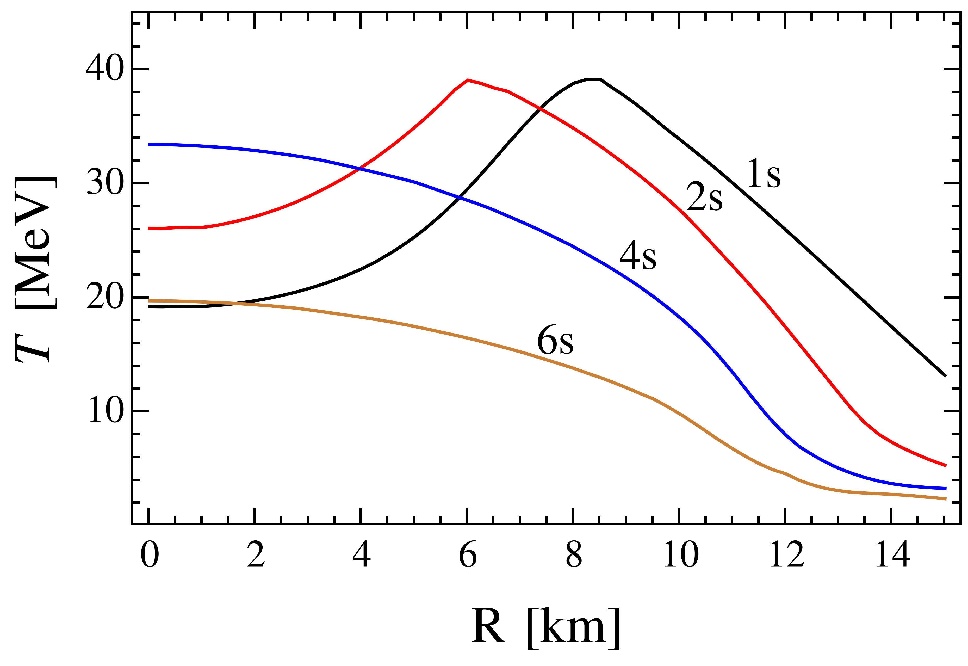
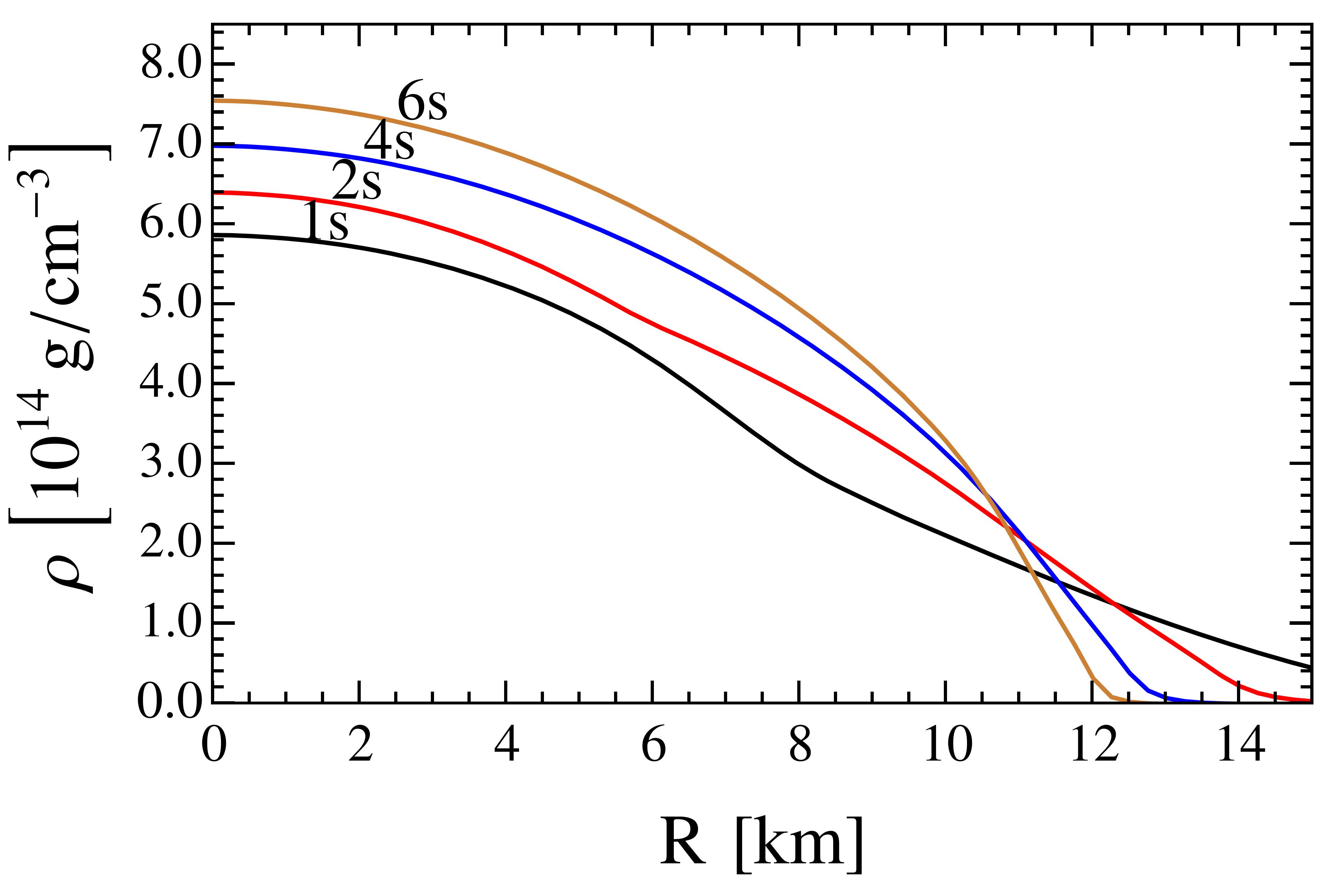
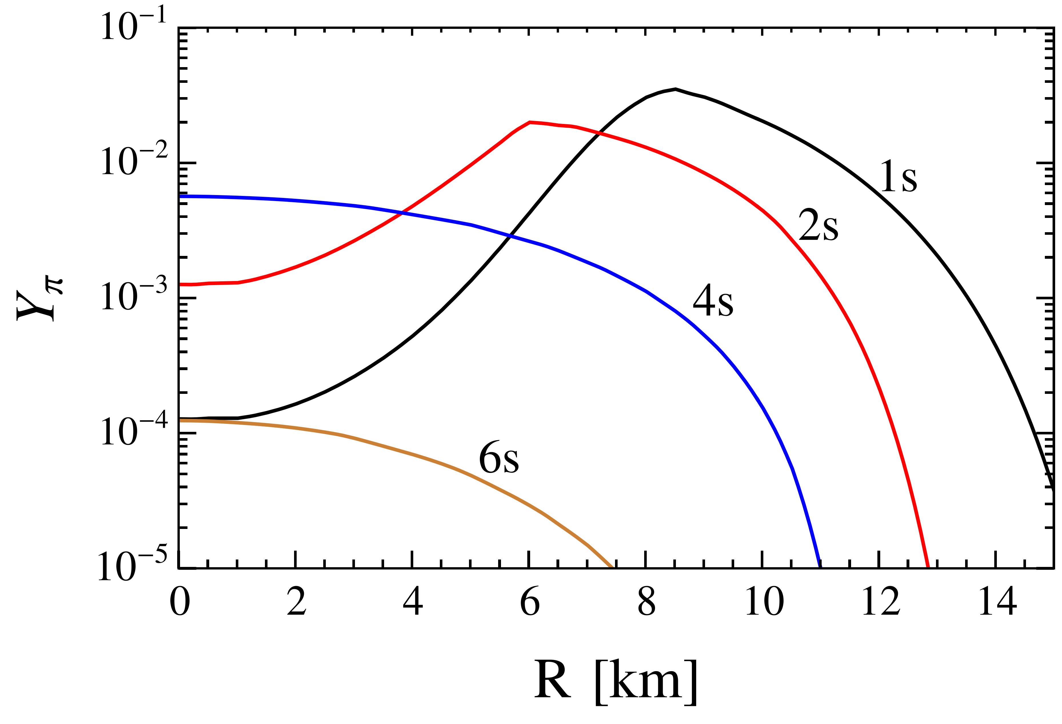
Figure 9: Radial profiles of the temperature $T$ (upper panel), density $\rho$ (central panel) and pion fraction $Y_{\pi}$ (lower panel) for our benchmark SN model SFHo-s18.8 at different post-bounce times.

We show in Fig. 9 the radial profile of the temperature (upper panel), density (central panel) and pion fraction (lower panel), at post-bounce times $t=1$ s (black), $t=2$ s (red), $t=4$ s (blue) and $t=6$ s (brown) for our benchmark model. In the early-cooling phase, at $t=1-2$ s, the highest temperature ($T_{\rm max}\approx 40$ MeV) is reached at $R\approx 6-9$ km, while at late time ($t\gtrsim 4$ s) the temperature is peaked in the center ($T_{\rm max}\approx 32$ MeV at $t=4$ s and $T_{\rm max}\approx 20$ MeV at $t=6$ s) and decreases at larger radii. On the other hand, due to the protoneutron star contraction, the inner-core density monotonically increases from $\rho_{\rm max}\approx 6\times 10^{14}~{\rm g}/\operatorname{cm}^{3}$ at $t=1$ s to $\rho_{\rm max}\approx 8\times 10^{14}~{\rm g}/\operatorname{cm}^{3}$ at $t=6$ s. Finally, the pion fraction peaks in coincidence to the temperature peak and follows the time behavior of the temperature profile. In particular, the highest pion abundances in the core are expected to be at $t=1-2$ s, where they can reach values as high as $Y_{\pi}\sim 2-3\,\%$, while they are significantly suppressed at later times. These conditions lead to the time evolution of the axion emission spectrum for our benchmark model, described in Appendix A.1 of Ref. [46]. In this work, we perform our analysis using the axion emission spectrum integrated over 10 s after the core bounce.

Appendix B Angular Separations between SN Candidates

In this appendix we give details on the angular separation between all the stars presented in Tab. 1. The stars are identified by their index, defined in column $N$. The angular distance matrix is evidently symmetric

$$\Delta\Theta_{ij}=\begin{cases}0&\text{if }i=j,\\ \Delta\theta_{ij}&\text{if }i<j,\\ \Delta\theta_{ji}&\text{if }i>j,\end{cases}$$ (B.1)

where $\Delta\theta_{ij}=\Delta\theta_{ji}$. For the SN candidates considered in this work (cf. Table 1), the separation angles are shown in Tab. 5, where $i\in\left(1,\dots,14\right)$, $j\in\left(2,\dots,15\right)$. The minimal angular separation, i.e. the angular distance to the closest neighbour is highlighted.

Table 5: Angular distances between all the stars in Tab. 1. The stars are identified by the $i,~j$ indexes. Colored data indicate the smallest angle separation associated with each star.

$\Delta\theta_{ij}$	2	3	4	5	6	7	8	9	10	11	12	13	14	15
1	47.1	39.7	63.8	45.9	125.8	83.2	113.4	60.6	120.4	119.8	115.6	98.8	98.8	57.6
2		44.1	98.3	16.0	79.1	66.9	160.5	83.1	95.5	159.1	81.4	143.0	143.0	80.0
3			55.8	29.7	108.0	108.5	122.8	39.0	139.5	115.0	124.0	102.1	102.1	36.0
4				85.4	145.8	143.0	67.0	20.6	162.3	61.6	179.3	46.3	46.3	22.3
5					84.6	82.8	152.1	68.4	109.9	143.7	94.4	131.6	131.6	65.5
6						67.4	120.3	128.5	48.3	113.5	34.8	134.9	134.9	128.4
7							116.8	143.4	37.3	132.6	36.3	132.0	132.0	140.2
8								85.2	96.9	18.6	113.2	20.7	20.7	87.9
9									176.8	75.9	159.6	64.6	64.6	3.3
10										105.3	17.5	117.5	117.5	175.2
11											118.8	21.4	21.4	79.1
12												133.9	133.9	157.8
13													0.0	67.2
14														67.2

References

- [1] S. Weinberg, A New Light Boson?, Phys. Rev. Lett. 40 (1978) 223.
- [2] F. Wilczek, Problem of Strong and Invariance in the Presence of Instantons, Phys. Rev. Lett. 40 (1978) 279.
- [3] R. D. Peccei and H. R. Quinn, CP Conservation in the Presence of Instantons, Phys. Rev. Lett. 38 (1977) 1440.
- [4] R. D. Peccei and H. R. Quinn, Constraints Imposed by CP Conservation in the Presence of Instantons, Phys. Rev. D 16 (1977) 1791.
- [5] L. F. Abbott and P. Sikivie, A Cosmological Bound on the Invisible Axion, Phys. Lett. B 120 (1983) 133.
- [6] M. Dine and W. Fischler, The Not So Harmless Axion, Phys. Lett. B 120 (1983) 137.
- [7] J. Preskill, M. B. Wise and F. Wilczek, Cosmology of the Invisible Axion, Phys. Lett. B 120 (1983) 127.
- [8] I. G. Irastorza et al., Towards a new generation axion helioscope, JCAP 06 (2011) 013.
- [9] IAXO Collaboration, A. Abeln et al., Conceptual design of BabyIAXO, the intermediate stage towards the International Axion Observatory, JHEP 05 (2021) 137 [2010.12076].
- [10] G. G. Raffelt, J. Redondo and N. Viaux Maira, The meV mass frontier of axion physics, Phys. Rev. D 84 (2011) 103008 [1110.6397].
- [11] S.-F. Ge, K. Hamaguchi, K. Ichimura, K. Ishidoshiro, Y. Kanazawa, Y. Kishimoto, N. Nagata and J. Zheng, Supernova-scope for the Direct Search of Supernova Axions, JCAP 11 (2020) 059 [2008.03924].
- [12] KamLAND Collaboration, K. Asakura et al., KamLAND Sensitivity to Neutrinos from Pre-Supernova Stars, Astrophys. J. 818 (2016) 91 [1506.01175].
- [13] SNEWS Collaboration, S. Al Kharusi et al., SNEWS 2.0: a next-generation supernova early warning system for multi-messenger astronomy, New J. Phys. 23 (2021) 031201 [2011.00035].
- [14] K. Rozwadowska, F. Vissani and E. Cappellaro, On the rate of core collapse supernovae in the milky way, New Astron. 83 (2021) 101498 [2009.03438].
- [15] H.-T. Janka, K. Langanke, A. Marek, G. Martinez-Pinedo and B. Mueller, Theory of Core-Collapse Supernovae, Phys. Rept. 442 (2007) 38 [astro-ph/0612072].
- [16] A. Mirizzi, I. Tamborra, H.-T. Janka, N. Saviano, K. Scholberg, R. Bollig, L. Hudepohl and S. Chakraborty, Supernova Neutrinos: Production, Oscillations and Detection, Riv. Nuovo Cim. 39 (2016) 1 [1508.00785].
- [17] P. Carenza, M. Giannotti, J. Isern, A. Mirizzi and O. Straniero, Axion Astrophysics, 2411.02492.
- [18] A. Lella, P. Carenza, G. Lucente, M. Giannotti and A. Mirizzi, Protoneutron stars as cosmic factories for massive axionlike particles, Phys. Rev. D 107 (2023) 103017 [2211.13760].
- [19] A. Lella, P. Carenza, G. Co’, G. Lucente, M. Giannotti, A. Mirizzi and T. Rauscher, Getting the most on supernova axions, Phys. Rev. D 109 (2024) 023001 [2306.01048].
- [20] A. Lella, E. Ravensburg, P. Carenza and M. C. D. Marsh, Supernova limits on QCD axionlike particles, Phys. Rev. D 110 (2024) 043019 [2405.00153].
- [21] M. Carena and R. D. Peccei, The Effective Lagrangian for Axion Emission From SN1987A, Phys. Rev. D 40 (1989) 652.
- [22] R. P. Brinkmann and M. S. Turner, Numerical Rates for Nucleon-Nucleon Axion Bremsstrahlung, Phys. Rev. D 38 (1988) 2338.
- [23] M. S. Turner, Dirac neutrinos and SN1987A, Phys. Rev. D 45 (1992) 1066.
- [24] G. G. Raffelt, Stars as laboratories for fundamental physics: The astrophysics of neutrinos, axions, and other weakly interacting particles. 5, 1996.
- [25] W. Keil, H.-T. Janka, D. N. Schramm, G. Sigl, M. S. Turner and J. R. Ellis, A Fresh look at axions and SN-1987A, Phys. Rev. D 56 (1997) 2419 [astro-ph/9612222].
- [26] P. Carenza, T. Fischer, M. Giannotti, G. Guo, G. Martínez-Pinedo and A. Mirizzi, Improved axion emissivity from a supernova via nucleon-nucleon bremsstrahlung, JCAP 10 (2019) 016 [1906.11844]. [Erratum: JCAP 05, E01 (2020)].
- [27] S. Stoica, B. Pastrav, J. E. Horvath and M. P. Allen, Pion mass effects on axion emission from neutron stars through NN bremsstrahlung processes, Nucl. Phys. A 828 (2009) 439 [0906.3134]. [Erratum: Nucl.Phys.A 832, 148 (2010)].
- [28] T. E. O. Ericson and J. F. Mathiot, Axion Emission from SN 1987a: Nuclear Physics Constraints, Phys. Lett. B 219 (1989) 507.
- [29] G. Raffelt and D. Seckel, Multiple scattering suppression of the bremsstrahlung emission of neutrinos and axions in supernovae, Phys. Rev. Lett. 67 (1991) 2605.
- [30] H.-T. Janka, W. Keil, G. Raffelt and D. Seckel, Nucleon spin fluctuations and the supernova emission of neutrinos and axions, Phys. Rev. Lett. 76 (1996) 2621 [astro-ph/9507023].
- [31] K. Springmann, M. Stadlbauer, S. Stelzl and A. Weiler, From Supernovae to Neutron Stars: A Systematic Approach to Axion Production at Finite Density, 2410.10945.
- [32] A. Caputo and G. Raffelt, Astrophysical Axion Bounds: The 2024 Edition, PoS COSMICWISPers (2024) 041 [2401.13728].
- [33] B. Fore and S. Reddy, Pions in hot dense matter and their astrophysical implications, Phys. Rev. C 101 (2020) 035809 [1911.02632].
- [34] P. Carenza, B. Fore, M. Giannotti, A. Mirizzi and S. Reddy, Enhanced Supernova Axion Emission and its Implications, Phys. Rev. Lett. 126 (2021) 071102 [2010.02943].
- [35] K. Choi, H. J. Kim, H. Seong and C. S. Shin, Axion emission from supernova with axion-pion-nucleon contact interaction, JHEP 02 (2022) 143 [2110.01972].
- [36] S.-Y. Ho, J. Kim, P. Ko and J.-h. Park, Supernova axion emissivity with (1232) resonance in heavy baryon chiral perturbation theory, Phys. Rev. D 107 (2023) 075002 [2212.01155].
- [37] P. Carenza, Axion emission from supernovae: a cheatsheet, Eur. Phys. J. Plus 138 (2023) 836 [2309.14798].
- [38] Garching core-collapse supernova research archive, https://wwwmpa.mpa-garching.mpg.de/ccsnarchive//.
- [39] G. Raffelt and D. Seckel, Bounds on Exotic Particle Interactions from SN 1987a, Phys. Rev. Lett. 60 (1988) 1793.
- [40] D. F. G. Fiorillo, M. Heinlein, H.-T. Janka, G. Raffelt, E. Vitagliano and R. Bollig, Supernova simulations confront SN 1987A neutrinos, Phys. Rev. D 108 (2023) 083040 [2308.01403].
- [41] A. Caputo, G. Raffelt and E. Vitagliano, Radiative transfer in stars by feebly interacting bosons, JCAP 08 (2022) 045 [2204.11862].
- [42] J. Engel, D. Seckel and A. C. Hayes, Emission and detectability of hadronic axions from SN1987A, Phys. Rev. Lett. 65 (1990) 960.
- [43] R. Bollig, W. DeRocco, P. W. Graham and H.-T. Janka, Muons in Supernovae: Implications for the Axion-Muon Coupling, Phys. Rev. Lett. 125 (2020) 051104 [2005.07141]. [Erratum: Phys.Rev.Lett. 126, 189901 (2021)].
- [44] A. Caputo, G. Raffelt and E. Vitagliano, Muonic boson limits: Supernova redux, Phys. Rev. D 105 (2022) 035022 [2109.03244].
- [45] A. Caputo, H.-T. Janka, G. Raffelt and E. Vitagliano, Low-Energy Supernovae Severely Constrain Radiative Particle Decays, Phys. Rev. Lett. 128 (2022) 221103 [2201.09890].
- [46] A. Lella, F. Calore, P. Carenza, C. Eckner, M. Giannotti, G. Lucente and A. Mirizzi, Probing protoneutron stars with gamma-ray axionscopes, JCAP 11 (2024) 009 [2405.02395].
- [47] M. Rampp and H. T. Janka, Radiation hydrodynamics with neutrinos: Variable Eddington factor method for core collapse supernova simulations, Astron. Astrophys. 396 (2002) 361 [astro-ph/0203101].
- [48] T. Sukhbold, S. Woosley and A. Heger, A High-resolution Study of Presupernova Core Structure, Astrophys. J. 860 (2018) 93 [1710.03243].
- [49] T. Fischer, P. Carenza, B. Fore, M. Giannotti, A. Mirizzi and S. Reddy, Observable signatures of enhanced axion emission from protoneutron stars, Phys. Rev. D 104 (2021) 103012 [2108.13726].
- [50] M. Mukhopadhyay, C. Lunardini, F. X. Timmes and K. Zuber, Presupernova neutrinos: directional sensitivity and prospects for progenitor identification, Astrophys. J. 899 (2020) 153 [2004.02045].
- [51] S. Healy, S. Horiuchi, M. Colomer Molla, D. Milisavljevic, J. Tseng, F. Bergin, K. Weil and M. Tanaka, Red Supergiant Candidates for Multimessenger Monitoring of the Next Galactic Supernova, Mon. Not. Roy. Astron. Soc. 529 (2024) 3630 [2307.08785].
- [52] M. Wenger et al., The simbad astronomical database, Astron. Astrophys. Suppl. Ser. 143 (2000) 9 [astro-ph/0002110].
- [53] K. M. Patton, C. Lunardini, R. J. Farmer and F. X. Timmes, Neutrinos from beta processes in a presupernova: probing the isotopic evolution of a massive star, Astrophys. J. 851 (2017) 6 [1709.01877].
- [54] KamLAND, Super-Kamiokande Collaboration, S. Abe et al., Combined Pre-supernova Alert System with KamLAND and Super-Kamiokande, Astrophys. J. 973 (2024) 140 [2404.09920].
- [55] Theia Collaboration, M. Askins et al., THEIA: an advanced optical neutrino detector, Eur. Phys. J. C 80 (2020) 416 [1911.03501].
- [56] IAXO Collaboration, E. Armengaud et al., Physics potential of the International Axion Observatory (IAXO), JCAP 06 (2019) 047 [1904.09155].
- [57] G. Raffelt and L. Stodolsky, Mixing of the Photon with Low Mass Particles, Phys. Rev. D 37 (1988) 1237.
- [58] K. van Bibber, P. McIntyre, D. Morris and G. Raffelt, Design for a practical laboratory detector for solar axions, Physical Review D 39 (1989) 2089.
- [59] S. Wilks, The large-sample distribution of the likelihood ratio for testing composite hypotheses, Annals of Mathematical StatisticsS 9 (1938) 60.
- [60] A. Ayala, I. Domínguez, M. Giannotti, A. Mirizzi and O. Straniero, Revisiting the bound on axion-photon coupling from Globular Clusters, Phys. Rev. Lett. 113 (2014) 191302 [1406.6053].
- [61] O. Straniero, A. Ayala, M. Giannotti, A. Mirizzi and I. Dominguez, Axion-Photon Coupling: Astrophysical Constraints, in 11th Patras Workshop on Axions, WIMPs and WISPs, pp. 77–81, 2015, DOI.
- [62] M. J. Dolan, F. J. Hiskens and R. R. Volkas, Advancing globular cluster constraints on the axion-photon coupling, JCAP 10 (2022) 096 [2207.03102].
- [63] J. Ruz et al., NuSTAR as an Axion Helioscope, 2407.03828.
- [64] R. Buras, M. Rampp, H. T. Janka and K. Kifonidis, Two-dimensional hydrodynamic core-collapse supernova simulations with spectral neutrino transport. 1. Numerical method and results for a 15 solar mass star, Astron. Astrophys. 447 (2006) 1049 [astro-ph/0507135].
- [65] H.-T. Janka, Explosion Mechanisms of Core-Collapse Supernovae, Ann. Rev. Nucl. Part. Sci. 62 (2012) 407 [1206.2503].
- [66] R. Bollig, H. T. Janka, A. Lohs, G. Martinez-Pinedo, C. J. Horowitz and T. Melson, Muon Creation in Supernova Matter Facilitates Neutrino-driven Explosions, Phys. Rev. Lett. 119 (2017) 242702 [1706.04630].