Comment on “Dark Energy from Time Crystals”

Abstract

It was recently proposed (https://arxiv.org/pdf/2502.08887) that the time crystal Lagrangian introduced by Shapere and Wilczek in 2012 could be a model of dark energy. I point out that the model has an instability that drives its energy density to negative values, which may render it unsuitable as a model of dark energy.

Recently Ref. Mersini-Houghton:2025ybm proposed that a higher-derivative scalar field theory, with a Lagrangian of the form

$${\cal L}=-\kappa X+\lambda X^{2}-V(\phi)\,,$$ (1)

could be a viable model of dark energy, where $X={\textstyle{1\over 2}}\partial_{\mu}\phi\partial^{\mu}\phi={\textstyle{1\over 2}}(\dot{\phi}^{2}-(\nabla\phi)^{2})$, and $\lambda,\kappa$ are positive constants. This is similar to a model that was proposed in Ref. Shapere:2012nq in the context of point particle mechanics, and dubbed “time crystals”, by virtue of spontaneously breaking time translation symmetry in a periodic fashion. In fact, in the absence of spatial derivatives, Eq. (1) is identical to the first model presented in Ref. Shapere:2012nq . In their paper, those authors point out that the relativistic version of the model suffers from gradient instabilities, that could be cured by considering instead a Lagrangian of the form $+\lambda X-\kappa X^{2}+\eta X^{3}$ whose energy is bounded from below. However, that was not the kind of model considered in Ref. Mersini-Houghton:2025ybm . Here I will explicitly show how the gradient instability in (1) leads to a loss of energy in the homogeneous mode that is supposed to provide the dark energy, driving it to negative values.

I start with a description of the dynamics of the homogeneous solutions, since we need to perturb around them to exhibit the instability. The Lagrangian equation of motion is

$$\ddot{\phi}(\kappa-\lambda\dot{\phi}^{2})={dV\over d\phi}\,,$$ (2)

which has a first integral of motion, the conserved energy density

$$E=V-{\textstyle{1\over 2}}\dot{\phi}^{2}\left(\kappa-{\textstyle{3\over 2}}\lambda\dot{\phi}^{2}\right)\,.$$ (3)

In Ref. Mersini-Houghton:2025ybm , the form of the potential was not specified (except for being positive semidefinite); I will assume $V={\textstyle{1\over 2}}m^{2}\phi^{2}$ for simplicity.

As Ref. Shapere:2012nq explained, the dynamics associated with (3) are those of a particle bouncing between two brick walls: the field velocity changes sign suddenly when it reaches a value that minimizes the kinetic energy, $\dot{\phi}^{2}=\kappa/(3\lambda)$. This can be understood by plotting the phase-space trajectories for fixed energy, as in Fig. 1. A strange feature of these trajectories is the presence of bifurcation points after the velocity jumps, where there is a choice of two possible solutions to join onto. At these points, $\dot{\phi}$ can either start decreasing or increasing, while $\phi$ can only either increase or decrease. The four branches, that are separated by the two bifurcation points plus their reflections, correspond to the four roots of the quartic equation (3) for $\dot{\phi}$.

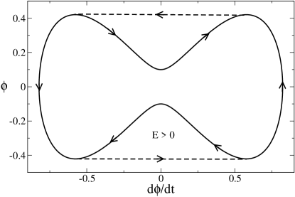
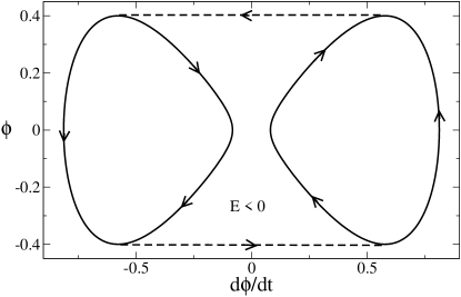
Figure 1: Phase space trajectories for closed orbits in the time crystal model. The dashed lines indicate where the field velocity discontinuously reverses its sign after hitting the “brick wall.” Left plot shows positive energy and right shows negative energy solutions. In either case there is a bifurcation point after the velocity changes sign, and the field has to “decide” which trajectory to follow. When $E=0$, an additional bifurcation point appears at the origin.

Next, we perturb the full equation of motion, including field gradients, around a spatially homogeneous solution $\phi_{0}(t)$. The result is

$$(\kappa - 3\lambda\dot{\phi}_{0}^{2})\,\delta\ddot{\phi}-(\kappa-\lambda\dot{\phi}_{0}^{2})\,\nabla^{2}\delta\phi$$ (4)

$$+ \left(6\lambda m^{2}\dot{\phi}_{0}\phi_{0}\over\kappa-\lambda\dot{\phi}_{0}^{2}\right)\delta\dot{\phi}-m^{2}\delta\phi=0\,.$$

In the damping term $\delta\dot{\phi}$ we used the zeroth order equation (2) to eliminate $\ddot{\phi}_{0}$. Except for $m^{2}=V^{\prime\prime}(\phi)$, all the coefficients are time-dependent since $\phi_{0}$ is oscillating. However, we are interested in the secular growth of $\delta\phi$, so we can average these coefficients over one period. The average value of $\dot{\phi}_{0}^{2}$ is of order $\kappa/(6\lambda)$. Moreover we can take $\delta\phi\sim e^{i(\omega t-\vec{k}\cdot\vec{x})}$. And the coefficient of the damping term averages to zero because $\phi_{0}\dot{\phi}_{0}$ changes sign midway through each oscillation. Then approximately

$$-{\textstyle{1\over 2}}\omega^{2}+{\textstyle{5\over 6}}k^{2}-{m^{2}\over\kappa}=0\,.$$ (5)

This gives imaginary frequencies for wave numbers in the instability band $k\lesssim m/\sqrt{\kappa}$, with

$$\omega\sim\pm i\sqrt{2m^{2}/\kappa-5k^{2}/3}\,.$$ (6)

To produce the unstable fluctuations, energy must be removed from the homogeneous mode, at a rate of order $m/\sqrt{\kappa}$. In the present peculiar theory, one should verify that these fluctuations actually carry positive energy in order to be sure that energy is really lost from the homogeneous mode. For this purpose, we expand the Lagrangian to second order in the perturbation around the homogeneous background. In the extreme case where $\dot{\phi}_{0}^{2}=\kappa/(3\lambda)$ which we will argue below is the endpoint of the evolution of the system, this gives

$$\delta^{2}{\cal L}={\textstyle{1\over 2}}\kappa(\delta\dot{\phi})^{2}+{\textstyle{1\over 3}}\kappa(\nabla\delta\phi)^{2}-{\textstyle{1\over 2}}m^{2}(\delta\phi^{2})\,.$$ (7)

Thus the kinetic energy of the fluctuation is positive, but the gradient energy is negative. Nevertheless, the total energy density of the fluctuations is given by

$$E_{\delta\phi}=\left[\kappa({\textstyle{1\over 2}}|\omega|^{2}-{\textstyle{1\over 3}}k^{2})+{\textstyle{1\over 2}}m^{2}\right](\delta\phi)^{2}\,,$$ (8)

and one can verify that for $k$ within the instability band, it is positive.

Notice that $\kappa$ is dimensionless, presumably $O(1)$, although Ref. Mersini-Houghton:2025ybm gives us no indication as to what values of $\kappa$, $\lambda$, or $m$ might be desirable. By evaluating the energy density $E$ at the turning point, where $\phi$ attains its maximum amplitude $\phi_{t}$, we have

$$E={\textstyle{1\over 2}}m^{2}\phi_{t}^{2}-{\kappa^{2}\over 12\lambda}\,.$$ (9)

As a consequence of the instability, $\phi_{t}$ decreases with time at the rate $|\omega|\sim m/\sqrt{\kappa}$, until the homogeneous mode degenerates into a zero-amplitude oscillation that has infinite frequency, with $\dot{\phi}_{0}$ continuously switching between $\pm\sqrt{\kappa/(3\lambda)}$. The energy density of the homogeneous component reaches a minimum value of $-{\kappa^{2}/(12\lambda)}$ and the Universe will evolve differently than expected from a typical dark energy model. In particular, both the energy density and the pressure $p=-5\kappa^{2}/(36\lambda)$ are negative, which will have peculiar consequences, perhaps only sensible if the contributions from the inhomogeneous components are also taken into account. Whether it is possible to choose values of parameters that postpone this until sufficiently far in the future (requiring $m/\sqrt{\kappa}\lesssim H_{0}$, the present Hubble rate), while allowing the model to be a viable description of dark energy in the present, would require further study to determine.

I thank S. Caron-Huot and L. Mersini-Houghton for enlightening discussions.

References

- (1) L. Mersini-Houghton, “Dark Energy from Time Crystals,” arXiv:2502.08887 [hep-ph].
- (2) A. Shapere and F. Wilczek, “Classical Time Crystals,” Phys. Rev. Lett. 109 (2012) 160402, arXiv:1202.2537 [cond-mat.other].