A geometric derivation of Noether’s theorem

Abstract

Nother’s theorem is a cornerstone of analytical mechanics, making the link between symmetries and conserved quantities. In this article, I propose a simple, geometric derivation of this theorem that circumvent the usual difficulties that a student of this field usually encounters. The derivation is based on the integration the differential form $dS=\mathbf{p}d\mathbf{q}-Hdt$, where $S$ is the action function, $\mathbf{p}$ the momentum and $H$ the Hamiltonian, over a closed path.

I Introduction.

Noether’s theorem [1] is one of the most celebrated theorem in physics, linking symmetries to conserved quantities.

Early in their education, physics undergraduates learn that the well-known conservation laws—momentum, energy, and angular momentum—are connected to symmetries in nature, such as translation in space and time, as well as rotation. This important relationship applies across all areas of physics and was established by the mathematician Emmy Noether in 1918. However, despite this beauty, they discover that most classical textbooks on mechanics don’t mention this theorem[2, 3], or devote a very small place to it[4, 5], or give a limited version of it [6] or postpone it to the very last section[7] (for an exception, see [8] ).

There are excellent books[9] dedicated to Noether’s theorem. Moreover, there are no shortage of articles in physics journal [10, 11, 12, 13] and public resources such as Wikipedia, to which the interested student can turn to. There are however several pitfalls for students before they can grasp the depth of Noether’s theorem. The symmetry of Noether’s theorem is not the symmetry of the potential energy, not even the symmetry of the Lagrangian ${\cal L}$ (which is harder to grasp, as the latter evaluates over trajectories, not point of space), but the invariance of ${\cal L}dt$ under a transformation. The classical examples of translation and rotation symmetry are slightly misleading, because the student could get the impression that these are simply those of the of potential energy.

The classical examples of applications of Noether’s theorem are also slightly underwhelming, as the usual conservation laws can be obtained simply by the method of cyclic or ignorable variables, where the shape of the potential is a guide for the choice of coordinates. Finally, when all the above pitfalls are overcome, students have to digest the heavy developments of the Rund-Trautman identity, making sense of derivation in respect to time versus the transformation parameter, apply that to an optimum trajectory, and discover that “miraculously”, most of the terms cancel out and lead to a simple expression where the momentum $\mathbf{p}$ and the Hamiltonian $H$ appear in a symmetric form reminiscent of relativity. For completeness, the Rund-Trautman derivation is detailed in subsection IV.2

These are in my opinion some of the reasons why most physics students are unaware of the meaning of this beautiful theorem. The Noether’s theorem however is so elegant, has such a deep meaning and makes connections between so many fields of physics that I believe it should be part of the background of any advanced undergraduate or graduate student. The theorem is also a first glimpse for students at Lie’s theory of continuous transformations, which was introduced in the 1880 precisely to study systematically the classification of differential equations according to their symmetries[14].

To overcome the difficulties enumerated above, I propose an alternative and simple derivation of the Noether’s theorem, highlighting its geometrical meaning. The derivation is based on the fundamental theorem of calculus that states that, for an analytical function $S$

$$\oint dS=0$$ (1)

where the integration is taken on a curve ${\cal C}$ inside the domain where $S$ is analytical (figure 3). The function $S\text{({q}},t)$ here is the action function that is the solution of the Hamilton-Jacobi (HJ) equation, i.e. the functional $S$ computed over actual trajectories, where

$$dS=\mathbf{p}d\mathbf{q}-Hdt$$ (2)

The curve ${\cal C}$ is formed of four branches, two of them being actual trajectories, where one is the transformed of the other under the transformation $(\phi_{\mathbf{q}},\phi_{t})$. If we suppose that the integral over these two branches are equal (to first order in a small parameter $\epsilon$), we must conclude that the integral over the two other branches must also be equal, leading naturally to Noether’s theorem that

$$I=\mathbf{p}\phi_{\mathbf{q}}-H\phi_{t}$$ (3)

is a conserved quantity along the trajectory. There is nothing miraculous in the simplifications of Rund-Trautman identity, these are a simple consequence of the fundamental theorem of calculus (1). This derivation is given in subsection IV.1. To be complete, the derivation using the Rund-Trautman identity is given in subsection IV.2. Before getting there however, I recall in section II the essential concepts of transformation groups and infinitesimal generators that are needed for this derivation. These concepts are the basis for the Lie theory of continuous transformations but can be presented simply without the full development of Lie groups. Section III is devoted to recalling the essential ingredients of analytical mechanics and its different formulations, mainly the Lagrangian and HJ formulation. Section VI is devoted to final concluding remarks. An appendix contains miscellaneous details that are recalled here for clarity.

II Point transformation and invariance

II.1 Definitions.

A continuous, one parameter transformation $T_{s}$ ($s\in\mathbb{R}$) transforms each point of the space $\boldsymbol{\mathbf{r}}$ into a new one

$$\boldsymbol{\mathbf{r}}^{\prime}=T_{s}(\boldsymbol{\mathbf{r}})$$ (4)

We restrict the discussion here to the case where transformations $T_{s}$ form a group [15]. Prime examples of such transformations are translations and rotations.

In order to characterize a transformation $T_{s}$, we only need to know its infinitesimal generator , i.e. how points are transformed for infinitesimal values of the parameter $s$. For example, in a two dimensional space referred to by the euclidean coordinates $(x,y)$, an infinitesimal rotation $\epsilon$ around the origin is characterized by

$$x^{\prime} = x-\epsilon y$$ (5)

$$y^{\prime} = y+\epsilon x$$ (6)

In vectorial notation, we write the infinitesimal transformation as

$$\boldsymbol{\mathbf{r}}^{\prime}=\boldsymbol{\mathbf{r}}+\epsilon\boldsymbol{\phi}(\boldsymbol{\mathbf{r}})$$ (7)

where the vector field $\boldsymbol{\phi}(\mathbf{r})$ is called the infinitesimal generator of the the transformation $T_{s}$ (figure 1). The vector field $\boldsymbol{\phi}(\mathbf{r})$ entirely characterizes the transformation $T_{s}$ : if we want to know the transformation for a finite value of $s$, we need to apply the transformation $T_{\epsilon}$ repeatedly, which is equivalent to solving the differential equation

$$\frac{d\boldsymbol{\mathbf{r}}}{ds}=\boldsymbol{\phi}(\boldsymbol{\mathbf{r}})$$ (8)

Solving the above equation for example for rotations (equations (5,6) ), we find the usual expression for 2d rotations :

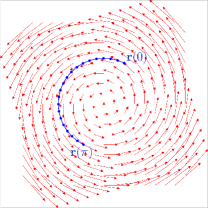
Figure 1: A vector field (red arrow) that transform (infinitesimally) each point into another $\boldsymbol{\mathbf{r}}^{\prime}=\boldsymbol{\mathbf{r}}+\epsilon\boldsymbol{\phi}(\boldsymbol{\mathbf{r}})$. In this example, the field corresponds to a rotation. To rotate by a finite quantity $\theta$, the infinitesimal transformation is applied $M$ times, where $M\epsilon=\theta$. This is equivalent to solving the differential equation (8), or finding the curve that is tangent to the vector field at each point (blue curve).

$$x(s) = x(0)\cos(s)-y(0)\sin(s)$$ (9)

$$y(s) = x(0)\sin(s)+y(0)\cos(s)$$ (10)

II.2 Symmetry and invariance.

Consider a function $f(\mathbf{r})$ defined over the points of space $\mathbf{r}=(r^{1},\ldots r^{n})$. The function is said to be invariant under a transformation $T_{s}$ if for every point of space,

$$f(T_{s}\mathbf{r})=f(\mathbf{r})$$ (11)

For the relation (11) to be valid, we only need it to be valid for an infinitesimal transformation :

$$f\left(\mathbf{r}+\epsilon\boldsymbol{\phi}(\boldsymbol{\mathbf{r}})\right)=f(\mathbf{r})$$ (12)

Developing to the first order in $\epsilon$, we then must have

$$\sum\frac{\partial f}{\partial r^{i}}\phi^{i}(\mathbf{r})=\left(\frac{\partial f}{\partial r^{1}},\ldots,\frac{\partial f}{\partial r^{n}}\right)\left(\begin{array}[]{c}\phi^{1}\\ \vdots\\ \phi^{n}\end{array}\right)=0$$ (13)

The application of the linear form $(\partial_{1}f,\ldots,\partial_{n}f)$ to the vector $\boldsymbol{\phi}$ must be null. The relation (13) is the condition for a function to be invariant under a transformation $\phi$.

For a given transformation $\phi$, solving the partial differential equation (13) gives the family of function that are invariant under this transformation. For example, consider a function $f(x,y)$ that is invariant under rotations. The infinitesimal generator of rotations is the vector field $\mathbf{\phi}=(-y,x)$, therefore we must have

$$-\frac{\partial f}{\partial x}y+\frac{\partial f}{\partial y}x=0$$ (14)

It is straightforward to check that any function of the form $f(x,y)=g(x^{2}+y^{2})$ is a solution of equation (14).

In classical mechanics, one of the coordinates, usually called time $t$, is distinguished from all the others called space $\mathbf{q}$. The vector field of a transformation is broken into its space and time components $\boldsymbol{\phi}(\mathbf{r})=\left(\boldsymbol{\phi}_{\mathbf{q}};\phi_{t}\right)^{T}$ ; this complicated notation better corresponds to our everyday experience, where we measure space by a stick and time by a clock. In the following sections, we will use this convention of classical mechanics.

III Formulations of mechanics

There are three different and equivalent formulations of analytical mechanics. We recall below the Lagrangian (see for example [2, 7]) and the Hamilton-Jacobi formulations (see for example [5], p248 or [16]). The Hamilton description, obtained through a Legendre transform of the Lagrangian, is not necessary for the present discussion of Noether’s theorem and is omitted.

III.1 Lagrangian formulations

The first approach to analytical mechanics is the Lagrangian one. In this formulation, a system is specified by a Lagrangian ${\cal L}(\mathbf{q},\dot{\mathbf{q}},t)$, where $\mathbf{q}(t)=\left(q^{1}(t),\ldots q^{n}(t)\right)^{T}$ is the position of the system at time $t$ in a given system of coordinates and $\dot{\mathbf{q}}=d\mathbf{q}/dt$ is its generalized velocity. To find the trajectory $\mathbf{q}(t)$ of the system one defines the momentum

$$\mathbf{p}=\frac{\partial{\cal L}}{\partial\dot{\mathbf{q}}}$$ (15)

and then uses the Euler-Lagrange equation

$$\frac{d}{dt}\mathbf{p}=\frac{\partial{\cal L}}{\partial\mathbf{q}}$$ (16)

to find the trajectories. In most problems of classical mechanics, equation (16) is a system of second order differential equations in $q^{i}(t)$.

It is important to precise the notations used here. Equation (15) is a short hand notation for

$$p_{i}=\frac{\partial{\cal L}}{\partial\dot{q}^{i}}$$ (17)

and $\mathbf{p}=(p_{1},\ldots,p_{n})$. Note that $\mathbf{p}$ is not a vector, but a linear form. In Linear algebra, vectors components are often grouped into a column vector, while linear forms are represented by a row vector. Here we make the distinction by using upper indexes for vector components (contravariant vector) and lower indexes for linear forms (covariant vectors). Applications of a linear form to a vector produces a scalar. For example,

$$\mathbf{p}\dot{\mathbf{q}}=\sum p_{i}\dot{q}^{i}$$ (18)

An important scalar quantity that is deduced from the Lagrangian is the Hamiltonian

$$H=\mathbf{p}\dot{\mathbf{q}}-{\cal L}$$ (19)

From the above relation, it is straightforward to deduce that (see subsection A.1)

$$\frac{dH}{dt}=-\frac{\partial{\cal L}}{\partial t}$$ (20)

if the Lagrangian does not contain time explicitly, then the Hamiltonian is conserved along a trajectory.

As an example, consider a two dimensional harmonic oscillator, where the Lagrangian is given by

$${\cal L}=\frac{m}{2}\left(\dot{x}^{2}+\dot{y}^{2}\right)-\frac{k}{2}\left(x^{2}+y^{2}\right)$$ (21)

The momentum is $\mathbf{p}=m(\dot{x},\dot{y})$ and the Hamiltonian is therefore

$$H=\frac{m}{2}\left(\dot{x}^{2}+\dot{y}^{2}\right)+\frac{k}{2}\left(x^{2}+y^{2}\right)$$ (22)

As we will see in the next section, the generalized $n+1$ linear form

$$(\mathbf{p},-H)$$ (23)

plays the central role in the Noether’s theorem : If the vector field $\left(\mathbf{\phi_{\mathbf{q}}};\phi_{t}\right)^{T}$ is the infinitesimal generator of a symmetry of the system, the conserved quantity along a trajectory is the scalar

$$(\mathbf{p},-H)\left(\begin{array}[]{c}\mathbf{\phi_{\mathbf{q}}}\\ \phi_{t}\end{array}\right)=\mathbf{p}\phi_{\mathbf{q}}-H\phi_{t}$$ (24)

Note that, as mentioned in the previous section, the term “generalized” is an exaggeration. Classically, one coordinate, called time $t$, is distinguished from the others, called space $\mathbf{q}$ and therefore various objects such as vectors and linear forms are broken into their time and space components, hiding the symmetry of the notations. The linear form $(\mathbf{p},-H)$ is widely used in special relativity : its transpose $(\mathbf{p},H)^{T}$ for a particle is called the four-vector momentum ; The sign (-) is the signature of our space-time.

Note also that the Lagrangian is not unique and is defined up a to a total derivative. If ${\cal L}(\mathbf{q},\dot{\mathbf{q}},t)$ describes a system and gives its trajectories, the Lagrangian

$${\cal L}^{\dagger}(\mathbf{q},\dot{\mathbf{q}},t)={\cal L}(\mathbf{q},\dot{\mathbf{q}},t)+\frac{d}{dt}F(\mathbf{q},t)$$ (25)

describes the same system and gives the same trajectories (see A.2). This indeterminacy in the Lagrangian introduces also an additional term in the most general statement of Noether’s theorem, which we will consider in A.2.

III.2 Hamilton-Jacobi formulation.

The Euler-Lagrange equation (16) is a consequence of an “extremum” concept. Given a functional $S$ of trajectories, called the “action”

$$S[\mathbf{q}(t)]=\int_{A}^{B}{\cal L}(\mathbf{q},\dot{\mathbf{q}},t)dt$$ (26)

where $A=(\mathbf{q}_{0},t_{0})$ and $B=(\mathbf{q}_{1},t_{1})$ are two end points of the curves, the trajectory followed by a system is one that corresponds to the extremum of the action. Such a trajectory is shown to obey the Euler-Lagrange equation (16).

On the other hand, if we know the real trajectories, $S=S(\mathbf{q}_{1},t_{1})$ becomes a simple function of the points in space, given an initial condition. The function $S$ is computed by evaluating the integral (26) over the known trajectories, themselves computed from the Euler-Lagrange equation (16). We can envisage $S(\mathbf{q}_{1},t_{1})$ as a wave front at time $t_{1}$ in analogy with geometrical optics.

As in the case of geometrical optics (which is a particular case of analytical mechanics), there is a duality between trajectories and wave fronts[16]. For optics, the duality was first developed by Huygens [17] in 1690 and it was fully integrated into analytical mechanics by Hamilton and Jacobi[18].

By duality, we mean that if we know the the action function $S(\mathbf{q},t)$ at all points of the space, we can deduce the trajectories (figure 2). The action function is related to the generalized momentum (23) through the relations (see A.3) :

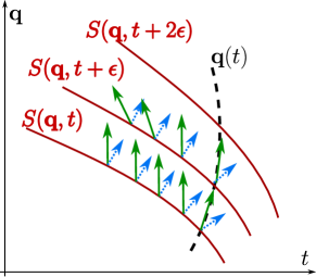
Figure 2: Computing the trajectories from the action $S(\mathbf{q},t)$ (here schematized by a 2d red contour plot). At each point, the momentum $(\mathbf{p},-H)=(\partial S/\partial\mathbf{q},\partial S/\partial t)$ (in blue) can be computed ; knowing $\mathbf{p}$, we can compute, from relation (15) the tangent to the trajectory $(\dot{\mathbf{q}},1)^{T}$ (in green). The trajectory (in black) is found by following a given line of tangents.

$$\frac{\partial S}{\partial\mathbf{q}} = \mathbf{p}$$ (27)

$$\frac{\partial S}{\partial t} = -H$$ (28)

Therefore, at each point of space, $(\mathbf{p},-H)$ is known. Knowing $\mathbf{p}$, we can find $\dot{\mathbf{q}}$ by solving the equation (15), which is usually an algebraic expression ; knowing $\dot{\mathbf{q}}(\mathbf{q},t)$, we solve the first degree ODE to find $\mathbf{q}(t)$ (figure 2).

The action $S(\mathbf{q},t)$ itself is computed from a first order nonlinear partial differential equation equation called the Hamilton-Jacobi equation (see A.3). The Hamilton-Jacobi approach, in the words of Arnold[5], is “[…] the most powerful method known for the exact integration [of Hamilton equations]”. The aim of this article is not to study the H-J approach (see for more details for example [16]). For the discussion of Noether’s theorem, we only need to know that the function $S(\mathbf{q},t)$ exists, is computable and analytical. Moreover, its differential, according to relations (27,28) is

$$dS=\mathbf{p}d\mathbf{q}-Hdt$$ (29)

which is the linear form (23) we briefly discussed in the previous subsection.

IV Noether’s theorem

There are various formulation of the Noether’s theorem. The simplest one, in our opinion, is the following:

If the action

$$S=\int_{A}^{B}{\cal L}(\mathbf{q},\dot{\mathbf{q}},t)dt$$ (30)

remains invariant under an infinitesimal transformation

$$\mathbf{\Phi=}(\mathbf{\phi}_{\mathbf{q}},\mathbf{\phi}_{t})$$ (31)

then the quantity

$$I=(\mathbf{p},-H)\left(\begin{array}[]{c}\mathbf{\phi_{\mathbf{q}}}\\ \phi_{t}\end{array}\right)=\mathbf{p}\phi_{\mathbf{q}}-H\phi_{t}$$ (32)

is conserved along the trajectory taken by the system.

The invariance means that under the transformation

$$\mathbf{q}^{\prime} = \mathbf{q}+\epsilon\mathbf{\phi_{\mathbf{q}}}$$ (33)

$$t^{\prime} = t+\epsilon\phi_{t}$$ (34)

We must have $S^{\prime}=S$ to the first order in $\epsilon$, or in other words,

$${\cal L}(\mathbf{q}^{\prime},\dot{\mathbf{q}^{\prime}},t^{\prime})dt^{\prime}={\cal L}(\mathbf{q},\dot{\mathbf{q}},t)dt$$ (35)

to the first order in $\epsilon$. This obviously implies that if $\mathbf{q}(t)$ is an extremum of the functional $S$, then $\mathbf{q}^{\prime}(t^{\prime})$ is an extremum of $S^{\prime}$ : the transformation (31) transforms extremum trajectories into extremum trajectories.

Let us precise the contour of Noether’s theorem. This theorem allows us, if we know of a symmetry, to deduce the conserved quantities. It does not allow us to find the symmetries in a efficient way ; for this purpose, there are other methods such as canonical transformation or the HJE equation. Moreover, it states that to a given symmetry a conserved quantity is associated. The converse however is not generally true, all conserved quantities do not derive from a symmetry, and not all transformations that transform a trajectory into a trajectory conserve the Lagrangian[5, subsection 4.20].

Finally, the most general form of Noether’s condition allows for the Lagrangians difference to be equal to a total time derivative to the first order in $\epsilon$ :

$${\cal L}(\mathbf{q}^{\prime},\dot{\mathbf{q}^{\prime}},t^{\prime})\frac{dt^{\prime}}{dt}={\cal L}(\mathbf{q},\dot{\mathbf{q}},t)+\epsilon\frac{d}{dt}F(\mathbf{q},t)$$ (36)

in which case, the conserved quantity along a trajectory is

$$\mathbf{p}\phi_{\mathbf{q}}-H\phi_{t}-F(\mathbf{q},t)$$ (37)

This generalization is considered in A.2.

IV.1 H-J Approach

Consider the action function $S(\mathbf{q},t)$ as defined in subsection IV.1, i.e. as the integral of the Lagrangian from an initial point $(\mathbf{q}_{0},t_{0})$ to the point $(\mathbf{q},t)$ over optimal paths. The hypotheses of the Noether’s theorem is equivalent to stating that $S$ is invariant (up to an additive constant) under the transformation field $\Phi=(\phi_{\mathbf{q}},\phi_{t})$. Now, consider a given action function $S(\mathbf{q},t)$ and two close trajectories ${\cal C}$ and ${\cal C}^{\prime}$ that are associated to $S$, by the procedure described in subsection III.2, and where ${\cal C}^{\prime}$ is a transform of ${\cal C}$ by the field $\Phi=(\phi_{\mathbf{q}},\phi_{t})$ (figure 3). Let us define a closed path ${\cal P}=AA^{\prime}B^{\prime}BA$ where the branches $AB={\cal C}$ and $A^{\prime}B^{\prime}={\cal C}^{\prime}$.

By the virtue of the fundamental theorem of Calculus[19] (see also A.4), we know that for a function $S$ analytic in a domain ${\cal D}$, we have

$$\oint dS=0$$ (38)

where the integration path ${\cal P}$ is inside the domain ${\cal D}$. By the hypothesis of Noether’s theorem, we have

$$\int_{{\cal C}}dS=\int_{{\cal C}^{\prime}}dS$$ (39)

therefore, by virtue of theorem (38), we also must have

$$\int_{A}^{A^{\prime}}dS=\int_{B}^{B^{\prime}}dS$$ (40)

Along the $AA^{\prime}$ branch, $d\mathbf{q}=\epsilon\phi_{\mathbf{q}}$ and $dt=\epsilon\phi_{t}$. The integral along the $AA^{\prime}$ branch, to the first order in $\epsilon$, is then simply

$$\int_{A}^{A^{\prime}}dS=\epsilon\left(\mathbf{p}\phi_{\mathbf{q}}-H\phi_{t}\right)+o(\epsilon)$$ (41)

Therefore, the quantity

$$I=\mathbf{p}\phi_{\mathbf{q}}-H\phi_{t}$$ (42)

is conserved along the trajectory.

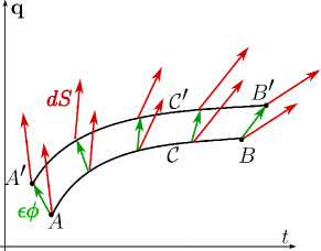
Figure 3: The integration path of $dS$ along a closed circuit ${\cal P}$. In red, the linear form $dS=\mathbf{p}d\mathbf{q}-Hdt$. The green vectors refer to the transformation $\Phi$.

IV.2 Lagrangian approach.

The Noether’s theorem in all sources I am aware of is demonstrated using the Lagrangian approach. This demonstration is equivalent to demonstrating that $dS$ is a closed form. We recall this demonstration here.

Consider a curve ${\cal C}$ parameterized by the coordinate $t$ and written as $\mathbf{q}(t)$ (figure 4). Consider a field of transformation $\mathbf{\Phi=}\left(\mathbf{\phi}_{\mathbf{q}}(\mathbf{q},t),\mathbf{\phi}_{t}(\mathbf{q},t)\right)$:

$$\mathbf{q}^{\prime} = \mathbf{q}+\epsilon\mathbf{\phi_{\mathbf{q}}}$$ (43)

$$t^{\prime} = t+\epsilon\phi_{t}$$ (44)

Along the curve ${\cal C}$, $\Phi$ itself can be parameterized by $t$

$$\Phi(t)=\Phi(\mathbf{q}(t),t)$$ (45)

and therefore, along the curve, the derivative $d\Phi/dt$ is well defined. Consider now two close points along the curve ${\cal C}$ with parameter $t_{1}$ and $t_{2}=t_{1}+dt$. The image of these points on ${\cal C}^{\prime}$ are given by $t^{\prime}_{1}=t_{1}+\epsilon\phi_{t}(t_{1})$ and

$$t^{\prime}_{2}=t_{2}+\epsilon\phi_{t}(t_{1}+dt)=t_{2}+\frac{d\phi_{t}}{dt}\epsilon dt$$ (46)

Therefore

$$dt^{\prime}=t^{\prime}_{2}-t^{\prime}_{1}=\left(1+\epsilon\frac{d\phi_{t}}{dt}\right)dt$$ (47)

By the same method, we obtain

$$d\mathbf{q}^{\prime}=d\mathbf{q}+\epsilon\frac{d\phi_{\mathbf{q}}}{dt}dt$$ (48)

Therefore, the quantity

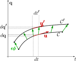
Figure 4: Scheme of transformation of a curve ${\cal C}$ into the curve ${\cal C}^{\prime}$ by the vector field $\Phi$. the vector $\mathbf{u}=(\dot{\mathbf{q}},1)$ in red is the tangent vector to the curve ${\cal C}$.

$$\dot{\mathbf{q}}(t)=\frac{\mathbf{q}(t+dt)-\mathbf{q}(t)}{dt}$$ (49)

transforms as

$$\dot{\mathbf{q}}^{\prime}(t)=\frac{d\mathbf{q}^{\prime}}{dt^{\prime}}=\dot{\mathbf{q}}(t)+\epsilon\left(\frac{d\phi_{\mathbf{q}}}{dt}-\dot{\mathbf{q}}\frac{d\phi_{t}}{dt}\right)$$ (50)

Recall that the hypothesis of the Nother’s theorem is that

$${\cal L}(\mathbf{q}^{\prime},\dot{\mathbf{q}^{\prime}},t^{\prime})dt^{\prime}={\cal L}(\mathbf{q},\dot{\mathbf{q}},t)dt$$ (51)

The relations (43,44,50) allow us to expand relation (51) to the first order in $\epsilon$ and write

$$\left[{\cal L}+\epsilon\left(\frac{\partial{\cal L}}{\partial\mathbf{q}}\mathbf{\phi_{\mathbf{q}}}+\frac{\partial{\cal L}}{\partial\dot{\mathbf{q}}}\left(\frac{d\phi_{\mathbf{q}}}{dt}-\dot{\mathbf{q}}\frac{d\phi_{t}}{dt}\right)+\frac{\partial{\cal L}}{\partial t}\phi_{t}\right)\right]$$

$$\times\left(1+\epsilon\frac{d\phi_{t}}{dt}\right)={\cal L}$$ (52)

Now, we suppose that the curve ${\cal C}$ is a trajectory of the system and obeys the Euler-Lagrange equation. Therefore, in the above relation, we can replace (figure 5) $\partial{\cal L}/\partial\dot{\mathbf{q}}=\mathbf{p}$ , $\partial{\cal L}/\partial\mathbf{q}=d\mathbf{p}/dt$ , $\partial{\cal L}/\partial t=dH/dt$ and ${\cal L}=\mathbf{p}\dot{\mathbf{q}}-H$. With these replacements, relation (52) is written, to the first order in $\epsilon$, as

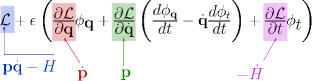
Figure 5: Scheme of replacements in expression (52).

$$\dot{\mathbf{p}}\phi_{\mathbf{q}}+\mathbf{p}\left(\dot{\phi}_{\mathbf{q}}-\dot{\mathbf{q}}\dot{\phi}_{t}\right)-\dot{H}\phi_{t}+\left(\mathbf{p}\dot{\mathbf{q}}-H\right)\dot{\phi}_{t}=0$$ (53)

We now only have to notice that the terms in $\mathbf{p}\dot{\mathbf{q}}\dot{\phi}_{t}$ cancel out in (53), and the remaining terms can be grouped into

$$\frac{d}{dt}\left(\mathbf{p}\phi_{\mathbf{q}}-H\phi_{t}\right)=0$$ (54)

In other words, the quantity between parenthesis in the above expression is conserved along a trajectory. These cancellations and grouping to give the final result would have seemed miraculous or mysterious, if we had not, in the previous subsection, given the geometric reason behind them.

V Applications

Let us suppose that we are given a certain symmetry and let us study its consequence, for some simple systems.

For a purely spatial symmetry where $\phi_{t}=0$, the conservation law reduces to

$$\mathbf{p}\boldsymbol{\phi}_{\mathbf{q}}=\text{constant}$$ (55)

For a pure translation symmetry where $\boldsymbol{\phi}_{\mathbf{q}}=\mathbf{u}$ (a constant vector), we have simply

$$\mathbf{p}\mathbf{u}=\sum p_{i}u^{i}=\text{constant}$$ (56)

i.e. the momentum in the direction of the vector $\mathbf{u}$ is conserved. For a rotation symmetry around the $z$ axis (relations 5,6), the conservation law is

$$L_{z}=m\left(-y\dot{x}+x\dot{y}\right)=\text{constant}$$ (57)

On the other hand, for a pure time translation where $\boldsymbol{\phi}_{\mathbf{q}}=\mathbf{0}$ and $\phi_{t}=a$, we have trivially

$$H=\text{constant}$$ (58)

We can use the Noether’s theorem in reverse and search for Lagrangians that are compatible with a given symmetry. Consider for example the Lagrangians for geodesics in two dimensional Euclidean geometry that are strictly compatible with a rotation symmetry and depend only on the first derivative :

$${\cal L}=f(\dot{y})$$ (59)

where $(x,y)$ are Cartesian coordinates of the plane, $\dot{y}=dy/dx$ ($x$ is the independent variable and $y$ the dependent one). For the rotation symmetry, $x^{\prime}=x-\epsilon y$, $y^{\prime}=y+\epsilon x$ and therefore, $\dot{y}^{\prime}=\dot{y}+\epsilon(1+\dot{y}^{2})$. Imposing the strict equality

$${\cal L}^{\prime}dx^{\prime}={\cal L}dx$$ (60)

and developing to the first order in $\epsilon$ results in the differential equation

$$(1+\dot{y}^{2})f^{\prime}(\dot{y})-\dot{y}f(\dot{y})=0$$ (61)

The solution of the above equation is $f(\dot{y})=C\sqrt{1+\dot{y}^{2}}.$ This form of the Lagrangian is not surprising, given the fact that rotations are precisely the transformations that preserve the usual distance.

For a Lorentz transformation

$$x^{\prime}=\gamma(x-vt)\,\,;\,\,t^{\prime}=\gamma(t-vx)$$ (62)

where $\gamma=1/\sqrt{1-v^{2}}$, the Infinitesimal generator is $\phi_{x}=-t$, $\phi_{t}=-x$. Repeating the above computation, one find that for a free particle, the Lagrangian compatible with Lorentz transform must be

$${\cal L}=C\sqrt{1-\dot{x}^{2}}$$ (63)

The above computations can be generalized without too much difficulty to Lagrangians of the form

$${\cal L}=f(\dot{y},y,t)$$ (64)

to find the general form of such a function. In particular, Lagrangians of the form ${\cal L}=a(\dot{y})+\dot{y}b(y,t)+c(y,t)$ will lead to the general form of Lagrangians for electromagnetic problems compatible with the requested symmetry. A detailed study of the Noether’s theorem for a charged particle in an electromagnetic field can be found in [20].

In principle, for a given Lagrangian, we can also look for the transformations that lead to invariance. This task however is achieved more efficiently by studying directly the Hamilton-Jacobi equation or by canonical transformations. Note that by these approaches, invariant quantities that are not obviously linked to symmetries can be recovered, as for example in the problem of attraction by two fixed center[21].

VI Conclusions

I have discussed in this article the geometrical meaning of the Noether’s theorem and its simple derivation from basics principles. The materials developed in this short article, which does not contain the usual mathematical complexities of Rund-Trautman approach found in most textbooks, can be covered in one lecture and I hope help students to get a basic understanding of one of the most elegant theorem of physics.

Acknowledgment.

I’m grateful to Cyril Falvo for crtical reading of the manuscript and fruitful discussions.

Appendix A Miscellaneous results.

A.1 Hamiltonian variation as a function of time.

The Hamiltonian is defined as

$$H=\mathbf{p}\dot{\mathbf{q}}-{\cal L}$$ (65)

Its variation along a trajectory is given by

$$\frac{dH}{dt}=\frac{d}{dt}\left(\mathbf{p}\dot{\mathbf{q}}\right)-\frac{d{\cal L}}{dt}$$ (66)

On one hand, we have

$$\frac{d{\cal L}}{dt} = \frac{\partial{\cal L}}{\partial\dot{\mathbf{q}}}\frac{d\dot{\mathbf{q}}}{dt}+\frac{\partial{\cal L}}{\partial\mathbf{q}}\frac{d\mathbf{q}}{dt}+\frac{\partial{\cal L}}{\partial t}$$ (67)

$$= \mathbf{p}\ddot{\mathbf{q}}+\dot{\mathbf{p}}\dot{\mathbf{q}}+\frac{\partial{\cal L}}{\partial t}$$ (68)

On the other hand,

$$\frac{d}{dt}\left(\mathbf{p}\dot{\mathbf{q}}\right)=\mathbf{p}\ddot{\mathbf{q}}+\dot{\mathbf{p}}\dot{\mathbf{q}}$$ (69)

Therefore, expression (66) is reduced to

$$\frac{dH}{dt}=-\frac{d{\cal L}}{dt}$$ (70)

A.2 Non-unicity of the Lagrangian and the general Noether’s theorem..

Consider two Lagrangians ${\cal L}(\mathbf{q},\dot{\mathbf{q}},t)$ and ${\cal L}^{\dagger}(\mathbf{q},\dot{\mathbf{q}},t)$ related through

$${\cal L}^{\dagger}(\mathbf{q},\dot{\mathbf{q}},t) = {\cal L}(\mathbf{q},\dot{\mathbf{q}},t)+\frac{d}{dt}F(\mathbf{q},t)$$ (71)

$$= {\cal L}(\mathbf{q},\dot{\mathbf{q}},t)+\dot{\mathbf{q}}\frac{\partial F}{\partial\mathbf{q}}+\frac{\partial F}{\partial t}$$ (72)

We have

$$\frac{\partial{\cal L}^{\dagger}}{\partial\dot{\mathbf{q}}}=\frac{\partial{\cal L}}{\partial\dot{\mathbf{q}}}+\frac{\partial F}{\partial\mathbf{q}}$$ (73)

and therefore

$$\frac{d}{dt}\left(\frac{\partial{\cal L}^{\dagger}}{\partial\dot{\mathbf{q}}}\right) = \frac{d}{dt}\left(\frac{\partial{\cal L}}{\partial\dot{\mathbf{q}}}\right)+\dot{\mathbf{q}}\frac{\partial^{2}F}{\partial\mathbf{q}^{2}}+\frac{\partial^{2}F}{\partial\mathbf{q}\partial t}$$ (74)

$$\frac{\partial{\cal L}^{\dagger}}{\partial\mathbf{q}} = \frac{\partial{\cal L}}{\partial\mathbf{q}}+\dot{\mathbf{q}}\frac{\partial^{2}F}{\partial\mathbf{q}^{2}}+\frac{\partial^{2}F}{\partial\mathbf{q}\partial t}$$ (75)

As a consequence,

$$\frac{d}{dt}\left(\frac{\partial{\cal L}^{\dagger}}{\partial\dot{\mathbf{q}}}\right)-\frac{\partial{\cal L}^{\dagger}}{\partial\mathbf{q}}=\frac{d}{dt}\left(\frac{\partial{\cal L}}{\partial\dot{\mathbf{q}}}\right)-\frac{\partial{\cal L}}{\partial\mathbf{q}}$$ (76)

Both Lagrangians give rise to the same equations of motion. Note that for clarity, we have used the vectorial notations instead of expressions containing explicitly the indexes. Usually, expressions such as (72) are written as

$${\cal L}^{\dagger}(\mathbf{q},\dot{\mathbf{q}},t)={\cal L}(\mathbf{q},\dot{\mathbf{q}},t)+\sum_{j}\dot{q}^{j}\frac{\partial F}{\partial q^{j}}+\frac{\partial F}{\partial t}$$ (77)

and for example

$$\frac{d}{dt}\left(\frac{\partial{\cal L}^{\dagger}}{\partial\dot{q}^{i}}\right)=\frac{d}{dt}\left(\frac{\partial{\cal L}^{\dagger}}{\partial\dot{q}^{i}}\right)+\sum_{j}\frac{\partial^{2}F}{\partial q^{i}\partial q^{j}}\dot{q}^{j}+\frac{\partial^{2}F}{\partial q^{i}\partial t}$$ (78)

The non-unicity of the Lagrangian has a consequence in the statement of the Noether’s theorem. In relation (35), the condition for the theorem to apply was stated as

$${\cal L}^{\prime}\frac{dt^{\prime}}{dt}={\cal L}$$ (79)

to the first order in $\epsilon$. As we saw above, the addition of a total time derivative does not change the trajectories, therefore we can now slightly relax the Noether’s condition and set the condition as

$${\cal L}^{\prime}\frac{dt^{\prime}}{dt}={\cal L}+\epsilon\frac{d}{dt}F(\mathbf{q},t)+o(\epsilon)$$ (80)

where $F$ is an arbitrary function. In this case, the computations of subsection IV.2 can be repeated to show that the conserved quantity in this case is

$$I=\mathbf{p}\phi_{\mathbf{q}}-H\phi_{t}-F$$ (81)

The geometric derivation of relation follows the computations of subsection IV.1 : Consider again the closed path ${\cal P}=AA^{\prime}B^{\prime}BA$ of figure 3. As mentioned, we must have $\oint dS=0$. If we have

$$\int_{A^{\prime}}^{B^{\prime}}dS-\int_{A}^{B}dS=\epsilon\int_{A}^{B}dF$$ (82)

we also must have

$$\int_{A}^{A^{\prime}}dS-\int_{B}^{B^{\prime}}dS=-\epsilon\int_{A}^{B}dF=-\epsilon\left(F(B)-F(A)\right)$$ (83)

which again leads to the generalized Noether’s charge of relation (81).

This generalized relation does not introduce anything new. To fix the idea, consider the two dimensional Lagrangian for movement in a central field

$${\cal L}=\frac{m}{2}\left(\dot{x}^{2}+\dot{y}^{2}\right)-U(x^{2}+y^{2})+\frac{d}{dt}F(x,y)$$ (84)

Without the additional total time derivative, the Lagrangian is invariant under rotational symmetry $\phi_{x}=-y$, $\phi_{y}=x$ and the conserved quantity is the angular momentum

$$L=m(-\dot{x}y+\dot{y}x)$$ (85)

With the additional term, the expression of $\mathbf{p}$ changes (for example, $p_{x}=m\dot{x}+\partial_{x}F$) and computing the Noether’s charge (relation 81) produces exactly the same angular momentum (relation 85) as the conserved quantity.

A.3 Variation of the function $S(\mathbf{q},t)$ and the Hamilton-Jacobi equation.

Consider an optimal trajectory $\mathbf{q}(t)$ with endpoints $(\mathbf{q}_{0},t_{0})$ and $(\mathbf{q}_{1},t_{1})$. Keeping the initial point fixed, the function $S(\mathbf{q}_{1},t_{1})$ is the action function. We are interested in computing the variation of $S()$ when the end point varies by a small quantity $(d\mathbf{q},dt)$ and obtain relations (27,28) of subsection III.2. We begin by keeping the final time fixed at $t_{1}$ but move the final position by $dq$ (figure 6). The trajectory $q(t)$ will vary by $\delta q(t)$ where $\delta q(t_{0})=0$ and $\delta q(t_{1})=dq$. The variation in $S$ is

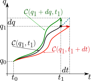
Figure 6: Varying the end points of a movement for computation of $\partial_{q}S$ and $\partial_{t}S$.

$$\delta S=\int_{t_{0}}^{t_{1}}\left\{\frac{\partial{\cal L}}{\partial\dot{q}}\delta\dot{q}+\frac{\partial{\cal L}}{\partial q}\delta q\right\}dt$$ (86)

However, the trajectories obey the Euler-Lagrange equation and we must have

$$\frac{\partial{\cal L}}{\partial q}=\frac{d}{dt}\frac{\partial{\cal L}}{\partial\dot{q}}$$

On the other hand, $\delta\dot{q}=d(\delta q)/dt$. Using these relations, we can rewrite equation (86) as

$$\delta S = \int_{t_{0}}^{t_{1}}\left\{\frac{\partial{\cal L}}{\partial\dot{q}}\frac{d\left(\delta q\right)}{dt}+\frac{d}{dt}\left(\frac{\partial{\cal L}}{\partial\dot{q}}\right)\delta q\right\}dt$$

$$= \int_{t_{0}}^{t_{1}}\frac{d}{dt}\left\{\frac{\partial{\cal L}}{\partial\dot{q}}\delta q\right\}dt$$

$$= \left[\frac{\partial{\cal L}}{\partial\dot{q}}\delta q\right]_{t_{0}}^{t_{1}}=\left.\frac{\partial{\cal L}}{\partial\dot{q}}\right|_{t_{1}}dq$$

As we have kept the final time fixed, $\delta S=\left(\partial S/\partial q\right)dq$ and therefore

$$\frac{\partial S}{\partial q}=\left.\frac{\partial{\cal L}}{\partial\dot{q}}\right|_{t_{1}}=p(t_{1})$$ (87)

If we vary the end point $q_{1}$, the relative variation in $S$ is the momentum $p$ at the end point, as stated in relation (27)

To compute the variation of $S$ as a function of the end point’s time, consider letting the original trajectory to continue along its optimal path. Then $dS={\cal L}dt.$ On the other hand

$$dS={\cal L}dt=\frac{\partial S}{\partial q}dq+\frac{\partial S}{\partial t}dt$$

Using our previous result (87), we have

$${\cal L}dt=pdq+\frac{\partial S}{\partial t}dt=\left(p\dot{q}+\frac{\partial S}{\partial t}\right)dt$$

and therefore

$$\frac{\partial S}{\partial t}={\cal L}-p\dot{q}=-H$$ (88)

which is relation (28).

The full derivation of the Hamilton-Jacobi equation can be found in ([16], we recall here only its form and use. The function $S(\mathbf{q},t)$ obeys the Hamilton-Jacobi equation ((HJE)

$$\frac{\partial S}{\partial t}+H\left(\mathbf{q},\frac{\partial S}{\partial\mathbf{q}},t\right)=0$$ (89)

which is a first order partial differential equation in $S$. The function $H$ is the Hamiltonian, written as a function of $\mathbf{q}$ and the momentum $\mathbf{p}$. Consider for example the 2d harmonic oscillator (relation 22)

$$H=\frac{m}{2}\left(\dot{x}^{2}+\dot{y}^{2}\right)+\frac{k}{2}\left(x^{2}+y^{2}\right)$$ (90)

and $\mathbf{p}=(p_{x},p_{y})=m(\dot{x},\dot{y})$. We rewrite the Hamiltonian as

$$H=\frac{1}{2m}\left(p_{x}^{2}+p_{y}^{2}\right)+\frac{k}{2}\left(x^{2}+y^{2}\right)$$ (91)

The HJ equation for the harmonic oscillator is then

$$\frac{\partial S}{\partial t}+\frac{1}{2m}\left(\left(\frac{\partial S}{\partial x}\right)^{2}+\left(\frac{\partial S}{\partial y}\right)^{2}\right)+\frac{k}{2}\left(x^{2}+y^{2}\right)=0$$ (92)

Even though HJE could seem complicated, there exist a systematic method to search for its solution, called canonical transformations (see for example [7, section 10.4]). When the potential function is separable $V(\mathbf{q})=\sum_{i}V_{i}(q_{i})$, we can look for a separable solution of the HJE.

A.4 Fundamental Theorem of calculus.

The fundamental theorem of calculus of integration of an exact “differential” for a multi-variable function over a closed path states that

$$\oint df=0$$ (93)

This theorem is known by various names to physics students such as the Stokes or the gradient theorem which is written in vector calculus as

$$\oint\nabla f.d\mathbf{r}=0$$

For example, if $f(\mathbf{r})$ is the electric potential, $\nabla f$ is the electric field and its circulation over a closed path is zero.

The most general approach to its demonstration is through the use of the language of differential forms[19] that provides a unified approach to integrals over curves, surfaces and higher order manifolds. I briefly summarize here the main results of this field that are related to relation (93). For a space referred by coordinates $\mathbf{x=}(x_{1},\ldots x_{n})$, a 1-form is an object such as

$$\omega=A_{1}(x_{1},\ldots x_{n})dx_{1}+\ldots A_{n}(x_{1},\ldots x_{n})dx_{n}$$ (94)

where $A_{i}(\mathbf{x})$ are functions of $n-$variables. A $2-$form involves elements such as $dx_{i}dx_{j}$ with the property that

$$dx_{i}dx_{j}=-dx_{j}dx_{i}\,\,\,;\,\,\,\,dx_{i}dx_{i}=0$$

and can be written as

$$\omega=\sum_{i,j,i\neq j}A_{ij}(\mathbf{x})dx_{i}dx_{j}$$ (95)

The definition can be generalized to $k-$forms. A zero-form is a scalar function. The exterior derivative transforms a $k-$form into a $(k+1)-$form. For example,

$$df=\sum_{i=1}^{n}\frac{\partial f}{\partial x_{i}}dx_{i}$$

The exterior derivative of a $1-$form such as $\alpha=A(\mathbf{r})dx_{k}$ is

$$d\alpha=\sum_{i=1,i\neq k}^{n}\frac{\partial A}{\partial x_{i}}dx_{i}dx_{k}$$

because, by definition, $dx_{i}dx_{i}=0$. This process can be used to define the exterior derivation of arbitrary $k-$form. In particular, for any differential form $\omega$

$$d(d\omega)=0$$ (96)

because such a derivation involves only terms of the form

$$\frac{\partial^{2}A}{\partial x_{i}\partial x_{j}}-\frac{\partial^{2}A}{\partial x_{j}\partial x_{i}}=0$$

A differential form that is the derivative of another one is called an exact form.

The integration of a differential $k-$form over a domain ${\cal D}$ corresponds to the usual definition of integration of multi-variable functions. The main theorem of integration of differential forms, known often as the generalized Stokes theorem states that

$$\int_{{\cal\partial D}}\omega=\int_{{\cal D}}d\omega$$ (97)

where $\partial D$ is the boundary of ${\cal D}$. Physics students often encounter specific cases of the above relations in vector calculus as Stokes and divergence (Ostrogradsky) theorems. For a function of one variable $f(x)$ integrated over the interval $[a,b]$, the above relation is the classical

$$\int_{a}^{b}df=f(b)-f(a)$$

Now, consider the exact form $\omega=df$ where $f(\mathbf{x})$ is a function a $n-$variable and its integration over a closed path $\partial{\cal D}$ :

$$\int_{{\cal\partial D}}df=\int_{{\cal D}}d(df)=0$$

by the virtue of relation (96).

References

- [1] Emmy Noether. Invariant Variation Problems (english translation by M. A. Tavel). Transport Theory and Statistical Physics, 1(3):186–207, January 1971.
- [2] Cornelius Lanczos. The Variational Principles of Mechanics. Dover Publications, 4th revised ed. édition edition, April 2012.
- [3] Richard P. Feynman, Robert B. Leighton, and Matthew Sands. The Feynman Lectures on Physics, Vol. I: The New Millennium Edition: Mainly Mechanics, Radiation, and Heat. Basic Books, new millennium ed. édition edition, September 2015.
- [4] L. D. Landau and E. M. Lifshitz. Mechanics: Volume 1. Butterworth-Heinemann, Amsterdam u.a, 3e édition edition, January 1976.
- [5] V. I. Arnol’d, K. Vogtmann, and A. Weinstein. Mathematical Methods of Classical Mechanics. Springer-Verlag New York Inc., New York, 2nd ed. 1989. corr. 4th printing 1997 édition edition, September 1997.
- [6] David Morin. Introduction to Classical Mechanics With Problems and Solutions. Cambridge India, first edition edition, January 2009.
- [7] Herbert Goldstein. Classical Mechanics. Pearson, Harlow, 3e édition edition, August 2013.
- [8] M G Calkin. Lagrangian and Hamiltonian Mechanics. WORLD SCIENTIFIC, July 1996.
- [9] Dwight E. Neuenschwander. Emmy Noether’s Wonderful Theorem. Johns Hopkins University Press, revised and updated edition edition, 2017.
- [10] Jean-Marc Lévy-Leblond. Conservation Laws for Gauge-Variant Lagrangians in Classical Mechanics. American Journal of Physics, 39(5):502–506, May 1971.
- [11] Edward A. Desloge and Robert I. Karch. Noether’s theorem in classical mechanics. American Journal of Physics, 45(4):336–339, April 1977.
- [12] Jozef Hanc, Slavomir Tuleja, and Martina Hancova. Symmetries and conservation laws: Consequences of Noether’s theorem. American Journal of Physics, 72(4):428–435, April 2004.
- [13] Gianluca Gorni and Gaetano Zampieri. Revisiting Noether’s Theorem on constants of motion. Journal of Nonlinear Mathematical Physics, 21(1):43–73, March 2014.
- [14] B. L. van der Waerden. A History of Algebra: From Al-Khwarizmi to Emmy Noether. Springer Verlag, Berlin Heidelberg, first edition edition, January 1985.
- [15] Anthony Zee. Group Theory in a Nutshell for Physicists. Princeton University Press, Princeton Oxford, March 2016.
- [16] Bahram Houchmandzadeh. The Hamilton–Jacobi equation: An alternative approach. American Journal of Physics, 88(5):353–359, April 2020.
- [17] A. E. Shapiro. Huygens’ ’Traité de la Lumière’ and Newton’s ’Opticks’: Pursuing and Eschewing Hypotheses. Notes and Records of the Royal Society of London, 43(2):223–247, 1989.
- [18] René Dugas. A History of Mechanics. Dover Publications, November 2012.
- [19] Harold M. Edwards. Advanced Calculus: A Differential Forms Approach. Birkhauser Verlag AG, Boston, 3e édition edition, November 1993.
- [20] Donald H. Kobe. Noether’s theorem and the work-energy theorem for a charged particle in an electromagnetic field. American Journal of Physics, 81(3):186–189, March 2013.
- [21] Holger Waalkens, Holger R. Dullin, and Peter H. Richter. The problem of two fixed centers: Bifurcations, actions, monodromy. Physica D: Nonlinear Phenomena, 196(3):265–310, September 2004.