A Study of the Provincial Road Networks of Canada as Complex Networks

Abstract

In this paper, we report on a study of the road networks of the provinces of Canada as complex networks. A number of statistical features have been analysed and compared with two random models. In addition, we have also studied the resilience of these road networks under random failures and targeted attacks.

1 Introduction

Statistical properties of protein-protein interaction networks, social networks, the world-wide web etc., have been studied in the framework of complex networks, leading to interesting insights into the function and properties of these networks. Motivated by this, we study the statistical properties of road networks of the 10 provinces of Canada. In addition, such a study would be an invaluable resource document for planning new transport infrastructure to address the needs of a dynamically growing population.

A random graph provides the mathematical model that serves as a benchmark or null hypothesis for studying real networks. Thus in this study, the statistics of each of the ten road networks is compared with a random graph, with the same number of nodes and edges, generated in Erdos-Renyi random graph model and another generated in the more general and versatile random graph model, known as the configuration model.

In the next section, we describe the data collection process; in the following section, we study some select statistical features of the road networks. Motivated by potentially catastrophic disruptions (climatic, for example) of a road network, in section 4 we investigate the resilience of the road networks under random and targeted disruptions.

2 Data Extraction Methodology

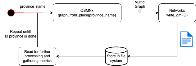
Figure 1: Flow Diagram of data extraction

The OSMnx [1] Python module is a powerful toolkit for extracting, modeling, and analyzing geographical networks, with a special emphasis on road networks. OSMnx uses data from OpenStreetMap to allow users to choose a geographical location, such as a province, and returns the accompanying road network as a graph. Figure 1 shows the data flow diagram (DFD) of the process that extracts a geographical network using the OSMnx library. The initial input is a province name to the function graph_from_place(province_name), which outputs a directed multi-graph $G(V,E)$. The nodes of $G$ represent the road intersections and the edges of $G$ represent the road segments that define this intersection. That $G$ is a directed multigraph means all the edges have directions and more than one edge can connect two arbitrary nodes $u,v$ of $G$. Next, using the versatile Networkx [5] python package used in the analysis of networks, graph $G$ is saved into the file system as a GML (Graph Modelling Language) file. GML is a text-based format commonly used for representing directed or undirected graphs, making it suitable for storing complex network structures like a province’s road network. This makes the task of analyzing the networks easier and also provides a way to replicate the results discussed in the subsequent sections.

3 Some Select Statistical Features

In any network analysis, the first metric that merits scrutiny is the number of nodes and edges in the network. Table 1 encapsulates this information about the road networks of all 10 provinces. We note that there are big differences in the number of road segments and the number of intersections among the provinces. Ontario, Quebec, Alberta, British Columbia and Saskatchewan have more than 100k nodes or intersections whereas the other provinces have fewer, with Prince Edward Island having the least of them all with just over 10k intersections. The number of edges or road segments also follows a similar pattern.

Province	Number of Nodes	Number of Edges
Nova Scotia	46,182	111,310
Ontario	359,535	938,322
Manitoba	70,694	197,154
Quebec	265,932	682,993
Alberta	256,831	631,772
Saskatchewan	126,405	348,263
New Brunswick	44,220	106,184
British Columbia	133,872	321,925
Prince Edward Island	10,078	25,172
Newfoundland and Labrador	35,329	80,704

Table 1: Sizes of the Province Road Networks

This is expected as the road network is built to cater to the population in these provinces and the population Table 2 below validates this correlation. The population data of each province has been obtained from the Statscan website [8].

Province	Number of Nodes	Number of Edges	Population
Ontario	359535	938322	15911285
Quebec	265932	682993	8984918
British Columbia	133872	321925	5431355
Alberta	256831	631772	4800768
Saskatchewan	126405	348263	1225493
Manitoba	70694	197154	1474439
Nova Scotia	46182	111310	1069364
New Brunswick	44220	106184	846190
Newfoundland and Labrador	35329	80704	540552
Prince Edward Island	10078	25172	176162

Table 2: Network Size versus Population Size

3.1 Clustering Coefficient

The local clustering coefficient of a node $i$ quantifies the cliquishness (or connectivity) of a node’s neighbourhood [3].

$$c_{u}=\frac{T(u)}{2(\deg^{\text{tot}}(u)(\deg^{\text{tot}}(u)-1)-2\deg^{\leftrightarrow}(u))}$$

where:

• $T(u)$ is the number of directed triangles through node $u$.

• $\deg^{\text{tot}}(u)$ is the sum of the in-degree and out-degree of node $u$.

• $\deg^{\leftrightarrow}(u)$ is the reciprocal degree of node $u$.

A global estimate of this measure for the entire graph is obtained by computing the average of the local clustering coefficients of all the vertices in the graph as below:

$$c=\frac{1}{N}\sum_{i\in V}c_{i}$$

where $c_{i}$ represents local clustering coefficient of vertex $i$ and $N$ represents the total number of nodes in the graph.

From table 3 we observe that the average local clustering coefficient is high for each province in comparison with their respective random graph models. We note that the global clustering coefficient also shows a similar trend. This indicates the presence of clusters in all the provincial road networks.

In [3], eight different clustering coefficients are defined, depending on the directedness of each edge that makes up a directed triangle incident on vertex $i$. These in turn are grouped into four types: cycle, middleman, in and out(see Fig. 2). Since the road networks of the provinces are essentially undirected graphs, we have not computed these different types of clustering coefficients.

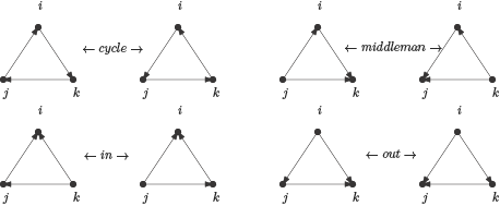
Figure 2: Directed triangles incident on vertex $i$

Graph Name	Global Clustering Coefficient
Nova Scotia	0.037522069345074884
Erdos Renyi Nova Scotia	4.543921329682012e-05
Configuration Model Nova Scotia	3.3073079389826195e-05
Ontario	0.048251411459397396
Erdos Renyi Ontario	7.202935777344378e-06
Configuration Model Ontario	9.834130990624786e-06
Manitoba	0.045504921394801494
Erdos Renyi Manitoba	2.9501882205081896e-05
Configuration Model Manitoba	3.431960953108434e-05
Quebec	0.046020266257265526
Erdos Renyi Quebec	8.090116275667468e-06
Configuration Model Quebec	1.1003529008131684e-05
Alberta	0.036883182912724945
Erdos Renyi Alberta	8.561449353254079e-06
Configuration Model Alberta	9.896261224955968e-06
Saskatchewan	0.03776036534494564
Erdos Renyi Saskatchewan	1.8667895136389256e-05
Configuration Model Saskatchewan	2.178372238891995e-05
New Brunswick	0.04130921468990875
Erdos Renyi New Brunswick	5.171839900269941e-05
Configuration Model New Brunswick	5.255109732721673e-05
British Columbia	0.039608137638506
Erdos Renyi British Columbia	2.1391931574792806e-05
Configuration Model British Columbia	1.4299373388652718e-05
Prince Edward Island	0.040585359107387045
Erdos Renyi Prince Edward Island	0.0001865929158050611
Configuration Model Prince Edward Island	0.0003859184078473619
Newfoundland and Labrador	0.03286609049537554
Erdos Renyi Newfoundland and Labrador	4.4805584871819415e-05
Configuration Model Newfoundland and Labrador	7.652555771664716e-05

Table 3: Global Clustering Coefficients

3.2 Average Shortest Distance

The next topological property studied is the average shortest distance that estimates the shortest distance between any two distinct nodes, picked at random. The distance measure here is the number of directed edges along the shortest path between any two nodes. This is calculated using the equation given below:

$$D=\frac{1}{N(N-1)}\sum_{s,t\in V}d(s,t)$$

where $d(s,t)$ is a measure of the shortest path from $s$ to $t$, $V$ is the set of all nodes in the graph and $N=|V|$.

If there is no path from a node $u$ to a node $v$, then the default shortest distance is set to a maximum integer value of 2147483647. From the table, we observe that, despite the size of the graph, the average shortest distance between vertices is small for all the provinces. Another intriguing observation is that for all the provinces the random graph constructed using the Erdos Renyi model has a significantly higher value, whereas the random graph generated using the configuration model has a value of the same order as the provinces. The Erdos Renyi model’s high values can be attributed to the presence of many unreachable paths.

Graph Name	Avg Shortest Distance
Nova Scotia	22.15222561
Erdos_Renyi_Nova Scotia	10341.70208
Configuration_Model_Nova Scotia	15.10254497
Ontario	4.900450389
Erdos_Renyi_Ontario	1073.49372
Configuration_Model_Ontario	4.268804188
Manitoba	44.67356109
Erdos_Renyi_Manitoba	4492.89145
Configuration_Model_Manitoba	34.36634661
Quebec	5.435196569
Erdos_Renyi_Quebec	1524.372326
Configuration_Model_Quebec	4.281091444
Alberta	16.01079995
Erdos_Renyi_Alberta	1789.856991
Configuration_Model_Alberta	13.86329372
Saskatchewan	20.55355934
Erdos_Renyi_Saskatchewan	2589.355722
Configuration_Model_Saskatchewan	6.988198076
New Brunswick	47.20932853
Erdos_Renyi_New Brunswick	11069.10252
Configuration_Model_New Brunswick	24.15828839
British Columbia	15.93452592
Erdos_Renyi_British Columbia	3651.772081
Configuration_Model_British Columbia	13.77707738
Prince Edward Island	295.8976174
Erdos_Renyi_Prince Edward Island	44953.9689
Configuration_Model_Prince Edward Island	147.9858415
Newfoundland and Labrador	30.97069985
Erdos_Renyi_Newfoundland and Labrador	15622.19806
Configuration_Model_Newfoundland and Labrador	18.92512441

Table 4: Average Shortest Distances

Average shortest distance values are ranked among provinces and are shown in the table 5. We observe that provinces with greater numbers of nodes and edges have smaller average shortest distances. Prince Edward Island has the highest value. This pattern is expected because a higher number of nodes and edges are required to support the population and their needs.

Province	Avg Shortest Distance
Ontario	4.900450389
Quebec	5.435196569
British Columbia	15.93452592
Alberta	16.01079995
Saskatchewan	20.55355934
Nova Scotia	22.15222561
Newfoundland and Labrador	30.97069985
Manitoba	44.67356109
New Brunswick	47.20932853
Prince Edward Island	295.8976174

Table 5: Average Shortest Distances Ranked

A small-world network has the following two distinctive characteristics (see[9]).

• High clustering coefficient when compared to a random network of the same size.

• The average node-to-node distance is approximately $\log(N)$

. All the province networks satisfy the first criteria, but not all provinces have an average shortest distance in the range of $\log(N)$. Specifically, the province of Prince Edward Island has a high average node-to-node distance.

3.3 Degree Distribution

The next parameter studied is the degree distribution of all the networks. In a directed graph there are two types of degrees for a vertex: in-degree and out-degree . In-degree is the number of the edges that come into the vertex and out-degree is the number of edges that leave the vertex. In this study, the degree of a vertex is defined as the sum of its in-degree and out-degree.

The degree distribution is the probability of finding a vertex with the given degree. It signifies the probability of occurrence of junctions with 2, 4, 6, etc. number of roads intersecting to form that junction. From Figures 3 and 4 below, we observe that, as expected, the Erdos-Renyi model graphs exhibit exponential degree distribution as represented by the blue bell curve, but the same is not true for the network of a province and its corresponding network in the configuration model. However, the latter two networks exhibit the same degree distribution. This can be attributed to the fact that the configuration model network graph is generated using the in-degree and out-degree sequence of that province. All the provinces exhibit a similar-looking degree distribution. This can be attributed to the fact that we are using junctions as nodes and the roads forming the junctions as edges.

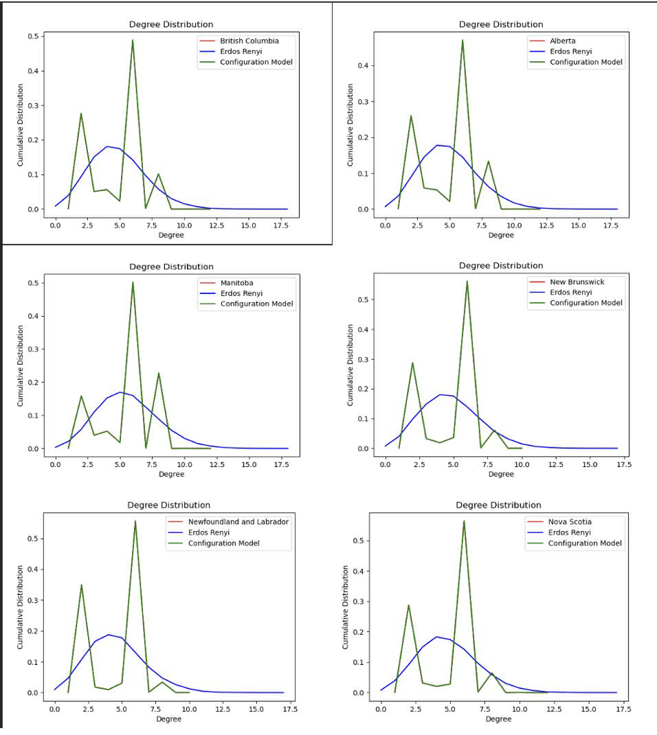
Figure 3: Degree distribution of each province

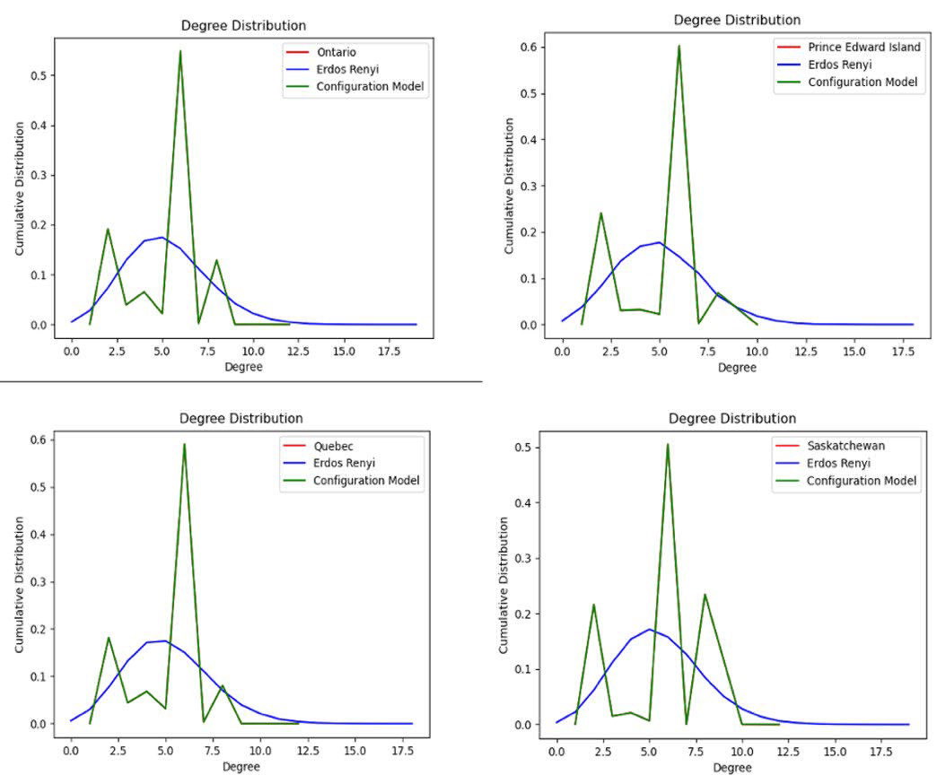
Figure 4: Degree distributions of each province

3.4 Average Degree of Neighbours

The average degree of neighbours is a measure used to identify the kind of neighbours a node associates with. It is a measure to identify if there is interdependence from one intersection to another. One should expect for the actual network of the province, the average degree of neighbours increases as the degree of the node increases. This is because the purpose of the transport network is to support movement and to prevent congestion there is a low possibility that an intersection’s neighbours have small degrees.

From Figure 5 below, we observe that in all the province networks the average degree of nearest neighbours of a node increases with its degree, whereas for the random networks, it is relatively constant. This agrees with our expectation and the assortativity measure studied in the next section, lends support to this.

Table 4 shows the global average degree of neighbours for all the networks.

Figure 5: Average degree of neighbours

Graph Name	Avg Degree of Neighbours
Nova Scotia	5.76932931
Erdos_Renyi_Nova Scotia	5.446416528
Configuration_Model_Nova Scotia	5.684723332
Ontario	5.648767403
Erdos_Renyi_Ontario	5.959860155
Configuration_Model_Ontario	5.889503094
Manitoba	5.456051606
Erdos_Renyi_Manitoba	6.208088796
Configuration_Model_Manitoba	6.273989996
Quebec	5.507781483
Erdos_Renyi_Quebec	5.792333836
Configuration_Model_Quebec	5.78562714
Alberta	5.309459965
Erdos_Renyi_Alberta	5.616876808
Configuration_Model_Alberta	5.846647238
Saskatchewan	5.60740285
Erdos_Renyi_Saskatchewan	6.117146874
Configuration_Model_Saskatchewan	6.310307503
New Brunswick	5.274978991
Erdos_Renyi_New Brunswick	5.580254002
Configuration_Model_New Brunswick	5.528243765
British Columbia	5.373841507
Erdos_Renyi_British Columbia	5.46544186
Configuration_Model_British Columbia	5.670169289
Prince Edward Island	5.394721234
Erdos_Renyi_Prince Edward Island	5.685891107
Configuration_Model_Prince Edward Island	5.751521122
Newfoundland and Labrador	5.18232645
Erdos_Renyi_Newfoundland and Labrador	5.275580474
Configuration_Model_Newfoundland and Labrador	5.422694977

Table 6: Average degree of neighbors by graph type and province

3.5 Topological Assortativity

In the previous section we observed that there is a positive correlation between degree of a node and average degree of its neighbours. Another parameter that estimates this correlation is Assortativity. Assortativity measures to which kind of neighbours a node prefers to attach. In other words it tries to answer the question on whether high degree nodes prefer to attach to other high degree node or not [7]. Following [4], we have computed four different types of assortativity, using the correlation formula below:

$$r(\alpha,\beta)=\frac{E^{-1}\Sigma_{i}(j_{i}^{\alpha}-\overline{j^{\alpha}})(k_{i}^{\beta}-\overline{k^{\beta}})}{\sigma^{\alpha}\sigma^{\beta}},$$

where $E$ is the set of all the edges in the network and $i$ is label of the $i$-th edge; the variables $\alpha$ and $\beta$ are in the set $\{in,out\}$, $j$ and $k$ are, respectively, the labels of the source and target vertex, $\overline{j^{\alpha}}$ is the mean of the $j_{i}^{\alpha}$ values taken over all the edges $E$, while $\sigma^{\alpha}=\sqrt{E^{-1}\Sigma_{i}(j_{i}^{\alpha}-\overline{j^{\alpha}})^{2}}$. The terms $\overline{j^{\beta}}$ and $\sigma^{\beta}$ have analogous definitons.

Road Network ID	In-In	Out-Out	In-Out	Out-In
Nova Scotia	-0.0009	-0.0009	0.0239	0.0004
Erdos_Renyi_Nova Scotia	-0.0001	0.0014	0.0044	0.0011
Configuration_Model_Nova Scotia	0.0012	0.0007	0.0011	0.0009
Ontario	0.1581	0.1587	0.1862	0.1572
Erdos_Renyi_Ontario	-0.0006	0.0013	0.0012	0.0001
Configuration_Model_Ontario	-0.0010	-0.0009	-0.0010	-0.0008
Manitoba	0.2119	0.2121	0.2366	0.2084
Erdos_Renyi_Manitoba	0.0022	-0.0017	0.0005	-0.0001
Configuration_Model_Manitoba	0.0011	.0015	0.0014	0.0009
Quebec	0.1197	0.1204	0.1591	0.1218
Erdos_Renyi_Quebec	-0.0007	0.0021	0.0008	0.0015
Configuration_Model_Quebec	0.0007	0.0002	0.0008	0.0001
Alberta	0.0.1268	0.0.1309	0.1590	0.1254
Erdos_Renyi_Alberta	0.0003	-0.0008	-0.0011	0.0009
Configuration_Model_Alberta	-0.0004	-0.0007	-0.0007	-0.0004
Saskatchewan	0.1102	0.1110	0.1208	0.1087
Erdos_Renyi_Saskatchewan	-0.0006	-0.0013	-0.0035	-0.0018
Configuration_Model_Saskatchewan	-0.0009	-0.0010	-0.0009	-0.0010
New Brunswick	-0.0364	-0.0372	-0.0070	-0.0316
Erdos_Renyi_New Brunswick	0.0003	0.0013	0.0000	0.0057
Configuration_Model_New Brunswick	0.0038	0.0032	0.0036	0.0034
British Columbia	0.0603	0.0604	0.0847	0.0608
Erdos_Renyi_British Columbia	0.0008	-0.0017	0.0022	-0.0021
Configuration_Model_British Columbia	0.0008	0.0008	0.0009	0.0007
Prince Edward Island	-0.0027	-0.0016	-0.0027	-0.0015
Erdos_Renyi_Prince Edward Island	0.0003	-0.0086	0.0004	-0.0025
Configuration_Model_Prince Edward Island	0.0216	0.0217	0.0486	0.0227
Newfoundland and Labrador	-0.1416	-0.1429	-0.1232	-0.1382
Erdos_Renyi_Newfoundland and Labrador	-0.0025	-0.0016	0.0050	-0.0018
Configuration_Model_Newfoundland and Labrador	-0.0091	-0.0091	-0.0094	-0.0088

Table 7: Assortativity Types

From the table 7, we observe that the both in-assortativity and out-assortativity coefficients are relatively high and are positive for all province networks barring the road network of Newfoundland and Labrador. This implies that there is assortative mixing in these networks except for the province of Newfoundland and Labrador and is consistent with the results from the graphs shown above.

4 Network Resilience

In the context of complex networks, network resilience involves studying how various types of networks, such as social networks, transportation systems, power grids, or computer networks, respond and adapt to disruptions (targeted attacks) or failures. Simulating attacks on a network can also be used to measure a network’s resilience.

There are two types network attack possible: one is a vertex-based attack and the other is an edge-based attack. Holme et al. [6] compared both types of attack for two real-world networks and four model networks, one of which is the Erdos Renyi model. Here we conduct a similar kind of study with an actual network and a corresponding random model network, generated using the configuration model.

The description of the various kinds of attacks and the inferences we can draw from these simulations are addressed in the following sections. For all the computations we have assumed that the road networks are all undirected.

4.1 Vertex Based Attack

A vertex-based attack identifies how the network behaves when vertices are removed from a network. When we remove a vertex $v$, all the incident edges are also removed.

There are many strategies available to remove vertices from a network. In this study, we discuss two of them: random removal of vertices and removal of vertices in descending order of vertex betweenness. The vertex betweenness measure identifies important vertices in the network.

The betweeeness centrality, $C_{B}(v)$, of a vertex $v$ is defined as below (see [2] for more details):

$$C_{B}(v)={\sum_{s\neq v\neq t}\frac{\sigma_{st}(v)}{\sigma_{st}}}\\$$ (1)

where:

• $\sigma_{st}$ is the total number of shortest paths from node $s$ to node $t$.

• $\sigma_{st}(v)$ is the number of those paths that pass through the node $v$.

• The sum is taken over all pairs of nodes $s$ and $t$, where $s\neq t$ and $s,t\neq v$.

In random vertex removal, we repeatedly remove 10% of the current vertices, selected at random from the network and to quantify network behaviour, the average shortest distance is then re-calculated for the residual (90%) vertices.

Another strategy we have explored is to remove repeatedly the top 10% of the current set of vertices in decreasing order of vertex betweenness and recalculate the average shortest distance of the residual (90%) vertices.

Both strategies are repeated for the random graph, generated using the configuration model.

We have plotted a graph that shows how the average shortest distance varies for each province in the targeted removal of vertices (6). From this figure, we can see that for Prince Edward Island there is a steep increase in the average shortest distance as vertices are removed. For the other provinces, the increase is gradual, implying other provinces are more resilient towards targeted vertex-based attack. Another insight we can gather from this plot is that bigger networks are more resilient. Understandably so, as in the bigger networks there are multiple ways to get to a target node.

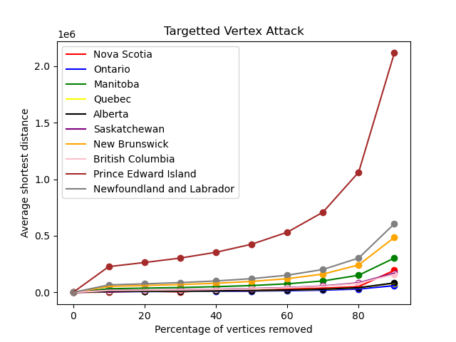
Figure 6: Average Shortest Distance vs Percentage of Nodes Removed

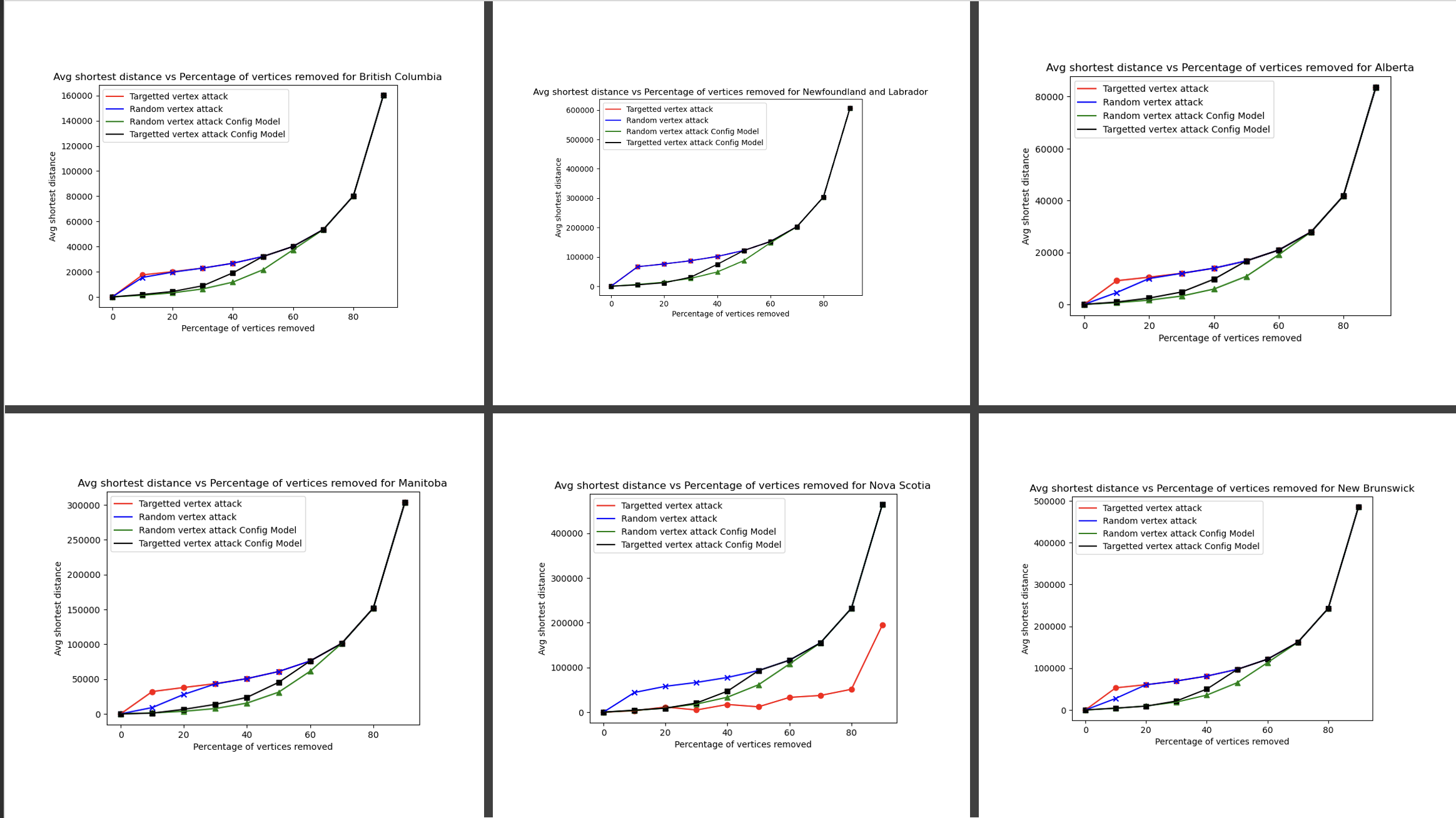
Figure 7: Random vs Targeted Vertex Attack

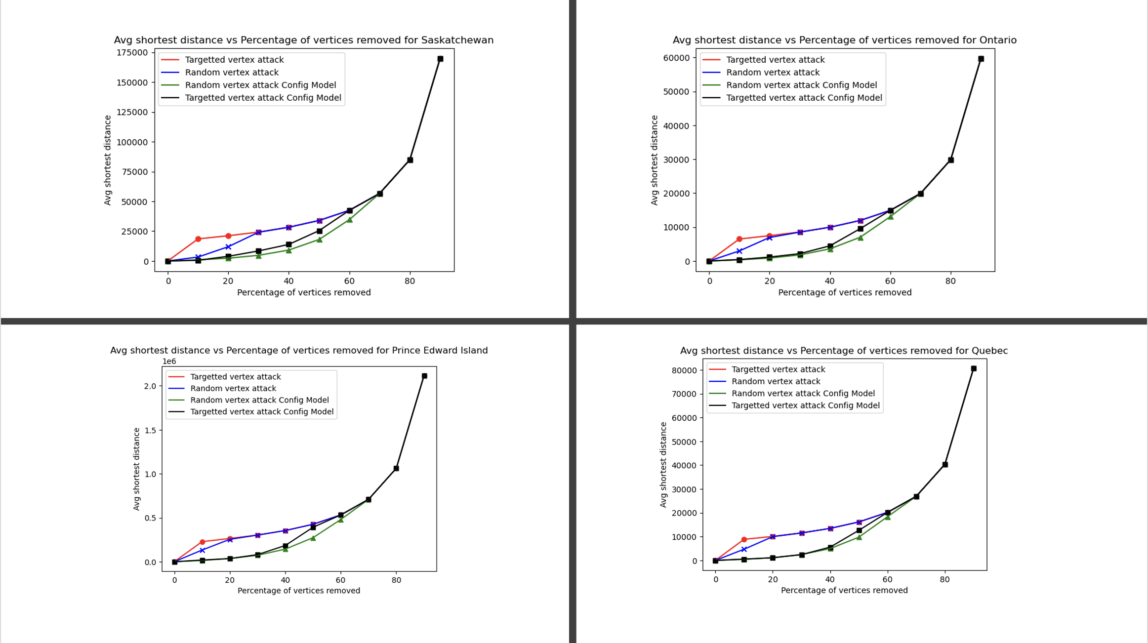
Figure 8: Random vs Targeted Vertex Attack

Figures 7 and 8 compare the impact on the average shortest distance of the random removal of vertices and targeted removal of vertices for the province networks and the random model networks.

Given the definition of vertex betweenness, one should expect the average shortest distance to increase at first because important vertices are removed and then follow the trend of random removal as more and more vertices are removed. This behaviour is seen in almost all provinces except for Nova Scotia.

Another observation is that in the random model, the impact of vertex removal is much more gradual when compared with the actual network. One possible explanation for this could be that in the actual network, the intersection and the road segments forming the intersection are interdependent. In contrast, in the random model, it is completely probabilistic.

4.2 Edge Based Attack

An edge-based attack quantifies how the network behaves on removal of edges from the network. Since the removal of an edge does not affect the vertices, repeated removal of edges leaves the network with isolated vertices.

As in the case of vertex removals, two strategies for removing edges are explored here: one is the random removal of edges, where in every iteration 10% of edges are selected at random and removed and is repeated until 90% of the edges are removed. In every iteration the new average shortest distance between vertices of the network is calculated and the graph of how it varies is plotted. Second is the targeted removal of edges where again 10% of the edges are removed in each iteration in the decreasing order of edge betweeness. Edge betweenness, $C_{B}(e)$, is calculated using the following formula [2]:

$$C_{B}(e)=\sum_{s\neq t}\frac{\sigma_{st}(e)}{\sigma_{st}}$$ (2)

where:

• $C_{B}(e)$ represents the betweenness centrality of an edge $e$.

• $\sigma_{st}$ is the total number of shortest paths from node $s$ to node $t$.

• $\sigma_{st}(e)$ is the number of those paths that pass through the edge $e$.

• The summation is taken over all pairs of nodes $s$ and $t$ in the graph, where $s\neq t$.

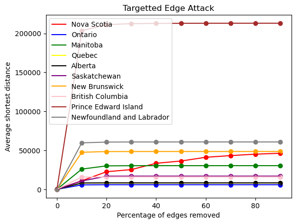
Figure 9: Avg Shortest Distance vs Percentage of edges Removed

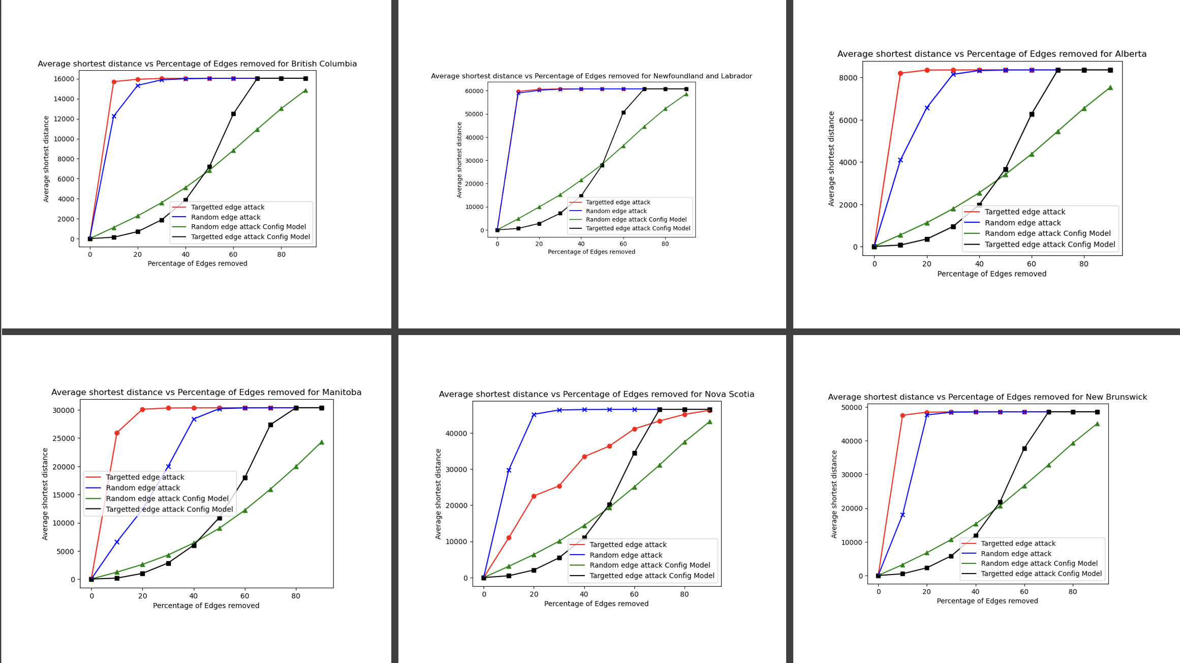
Figure 10: Random vs Targeted Edge Attack

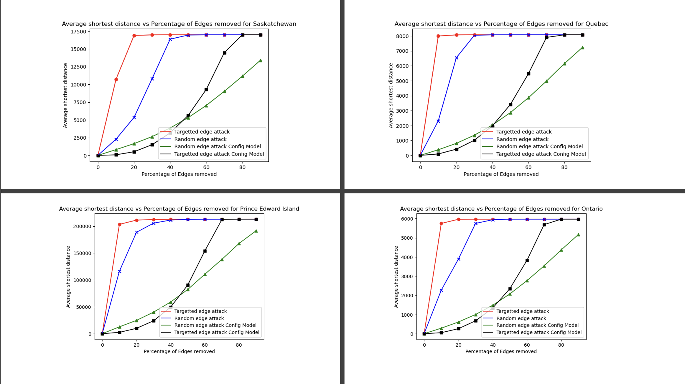
Figure 11: Random vs Targeted Edge Attack

Edge attacks as a whole have the same effect on province and random networks as vertex attacks seen in the previous section. Figure 9 shows that bigger networks are less susceptible to this kind of attack. Figures 10 and 11 also show that the average shortest distance increases gradually as compared with their respective actual province network. This strongly indicates that there is an interdependence between the vertices and edges of the network.

5 Conclusion

In this paper, the province networks of 10 provinces are extracted. Two random graphs, one using the Erdos Renyi model and the other using the configuration model with the same number of nodes and the same number of edges as the province network are generated. Parameters like clustering coefficient, degree distribution, average degree of neighbours and assortativity are compared among provinces and with their respective random graphs. An approach to quantify network resilience is discussed and is compared with one of the random models and among provinces. We found that the province network did not exhibit small-world properties, the larger the size of the province network more resilient it was to both vertex-based attacks and edge-based attacks and finally as expected there is an interdependence between edges and nodes of a network. We also noted that the configuration model was able to model the network more closely than Erdos-Renyi model.

References

- [1] Geoff Boeing. OSMnx: New methods for acquiring, constructing, analyzing, and visualizing complex street networks. Computers, Environment and Urban Systems, 65:126–139, 2017.
- [2] Ulrik Brandes. A faster algorithm for betweenness centrality. Journal of Mathematical Sociology, 25(2):163–177, 2001.
- [3] Giorgio Fagiolo. Clustering in complex directed networks. Phys. Rev. E, 76:026107, Aug 2007.
- [4] Jacob G. Foster, David V. Foster, Peter Grassberger, and Maya Paczuski. Edge direction and the structure of networks. Proceedings of the National Academy of Sciences, 107(24):10815–10820, 2010.
- [5] Aric Hagberg and Drew Conway. Networkx: Network analysis with python. URL: https://networkx. github. io, 2020.
- [6] Petter Holme, Beom Jun Kim, Chang No Yoon, and Seung Kee Han. Attack vulnerability of complex networks. Physical Review E, 65(5):056109, 2002.
- [7] Mark EJ Newman. The structure and function of complex networks. SIAM Review, 45(2):167–256, 2003.
- [8] Statistics Canada. Population estimates, quarterly. DOI, 2024.
- [9] Duncan J Watts and Steven H Strogatz. Collective dynamics of ‘small-world’ networks. Nature, 393(6684):440–442, 1998.