Work and heat exchanged during sudden quenches
of strongly coupled quantum systems

Abstract

How should one define thermodynamic quantities (internal energy, work, heat, etc.) for quantum systems coupled to their environments strongly? We examine three (classically equivalent) definitions of a quantum system’s internal energy under strong-coupling conditions. Each internal-energy definition implies a definition of work and a definition of heat. Our study focuses on quenches, common processes in which the Hamiltonian changes abruptly. In these processes, the first law of thermodynamics holds for each set of definitions by construction. However, we prove that only two sets obey the second law. We illustrate our findings using a simple spin model. Our results guide studies of thermodynamic quantities in strongly coupled quantum systems.

I Introduction

Quantum thermodynamics generalizes nineteenth-century principles about energy processing to quantum systems [1, 2, 3, 4, 5]. The field has advanced the studies of thermalization [6, 7], fluctuation theorems (extensions of the second law) [8, 9, 10, 11], thermal machines [12, 13, 14], energetic and informational resources [15, 16], and more. Controlled quantum systems have enabled experimental tests of quantum-thermodynamic predictions [17, 18, 19, 14, 20, 21, 22]. Yet how to define basic quantum-thermodynamic quantities (internal energy, work, heat, etc.) remains an open question [23, 24, 25, 26, 27, 28, 29, 30, 31, 32, 33, 34, 35, 36, 37, 38, 39, 40].

A standard thermodynamic setting features two subsystems: a system $S$ of interest and a thermal reservoir $R$. Typically, $S$ and $R$ satisfy the weak-coupling assumption: the subsystems’ interaction energy is negligible compared to the system’s and reservoir’s energies. The total system-reservoir internal energy then approximately equals the sum of the subsystems’ internal energies. This decomposition motivates the notion of heat as the energy lost by $R$ and gained by $S$ [41, 42].

Macroscopic systems obey the weak-coupling assumption. The reason is, the interaction energy scales as the system-reservoir boundary’s surface area, while the system’s and reservoir’s energies scale with the subsystems’ volumes. When $S$ is microscopic, this argument does not apply, and the weak-coupling assumption can break down. The weak-coupling assumption can break also under long-range interactions between a system’s and reservoir’s degrees of freedom (DOFs). These examples fall into the strong-coupling regime. In this regime, whether the interaction energy should be attributed to $S$ or to $R$, or somehow split between the two, is unclear . For classical systems, thermodynamic quantities (internal energy, entropy, heat, work, etc.) can nonetheless be defined in the strong-coupling regime consistently with the first and second laws of thermodynamics [44, 45, 46].

Several approaches have been proposed for extending the strong-coupling framework into the quantum regime [32, 33, 46, 47, 36, 48, 49, 50]. We collate three candidate definitions for internal energy [44, 51, 46]. Classically, these definitions lead to work and heat definitions that obey the second law. In the quantum case, we prove, only two definitions satisfy the second law; the third definition does not. (All internal-energy, heat, and work quantities in this paper are averages, i.e., expectation values.) Our proof applies to quench processes, in which the Hamiltonian changes abruptly. Such processes enable us to naturally partition the internal-energy change into work and heat. In summary, our results advance quantum thermodynamics, by defining quantities consistently with thermodynamic laws.

Our paper is organized as follows: Sections˜II and III specify the setup and three internal-energy definitions. Section˜IV describes our quench processes, as well as the partitioning of internal-energy changes into heat and work. Section˜V identifies the definitions that obey the second law. A spin model illustrates our findings in Sec.˜VI.

II Preliminaries

Consider a finite quantum system ${S\cup R}$ composed of subsystems $S$ and $R$. The Hamiltonian of ${S\cup R}$ is

$$\hat{H}_{{S\cup R}}\coloneqq\hat{H}_{S}\otimes\hat{\mathbbm{1}}_{R}+\hat{\mathbbm{1}}_{S}\otimes\hat{H}_{R}+\hat{V}_{{S\cup R}}\,.$$ (1)

$\hat{H}_{S}$ and $\hat{\mathbbm{1}}_{S}$ ($\hat{H}_{R}$ and $\hat{\mathbbm{1}}_{R}$) act on the Hilbert space of $S$ ($R$). $\hat{V}_{{S\cup R}}$ denotes the interaction between the subsystems. Throughout this paper, we call $S$ the system of interest or the system and call $R$ the reservoir. Also, we use the shorthand $\hat{H}_{{S\cup R}}=\hat{H}_{S}+\hat{H}_{R}+\hat{V}_{{S\cup R}}$.

We denote by $\hat{\rho}_{{S\cup R}}$ a state, pure or mixed, of ${{S\cup R}}$. The system’s reduced state follows from tracing out the reservoir: $\hat{\rho}_{S}\coloneqq{\mathrm{Tr}}_{R}\left(\hat{\rho}_{{S\cup R}}\right)$. We suppose that the global equilibrium state is the Gibbs state

$$\hat{\pi}_{{S\cup R}}\coloneqq\frac{e^{-\beta\hat{H}_{{S\cup R}}}}{Z_{{S\cup R}}}\,.$$ (2)

$\beta\coloneqq(k_{\rm B}T)^{-1}$ denotes the inverse temperature; $k_{\rm B}$, the Boltzmann factor; and $T$, the temperature. The partition function is $Z_{{S\cup R}}\coloneqq{\mathrm{Tr}}_{SR}(e^{-\beta\hat{H}_{{S\cup R}}})$. Consequently, the system’s equilibrium state is

$$\hat{\pi}_{S}\coloneqq{\mathrm{Tr}}_{R}\left(\hat{\pi}_{{S\cup R}}\right)\equiv\frac{e^{-\beta\hat{H}_{S}^{*}}}{Z_{S}^{*}}\,.$$ (3)

This equation introduces the Hamiltonian of mean force [46, 47, 52, 53, 54, 55],

$$\hat{H}_{S}^{*}\coloneq-\frac{1}{\beta}\ln{\left(\frac{{\mathrm{Tr}}_{R}\left(e^{-\beta\hat{H}_{{S\cup R}}}\right)}{{\mathrm{Tr}}_{R}\left(e^{-\beta\hat{H}_{R}}\right)}\right)}$$ (4)

and partition function $Z_{S}^{*}\coloneqq{\mathrm{Tr}}_{S}(e^{-\beta\hat{H}_{S}^{*}})$. Throughout this paper, we denote equilibrium states by $\hat{\pi}$, as in Eqs.˜2 and 3.

When $\hat{V}_{{S\cup R}}$ is negligible, one can treat $\hat{\pi}_{{S\cup R}}$ as a product $\hat{\pi}_{S}^{0}\otimes\hat{\pi}_{R}^{0}$ of system and reservoir Gibbs states,

$$\hat{\pi}_{S}^{0}\coloneqq\frac{e^{-\beta\hat{H}_{S}}}{Z_{S}}\quad\text{and}\quad\hat{\pi}_{R}^{0}\coloneqq\frac{e^{-\beta\hat{H}_{R}}}{Z_{R}}\,,$$ (5)

wherein $Z_{S}\coloneqq{\mathrm{Tr}}_{S}(e^{-\beta\hat{H}_{S}})$ and $Z_{R}\coloneqq{\mathrm{Tr}}_{R}(e^{-\beta\hat{H}_{R}})$. In this weak-coupling regime, $\hat{H}_{S}^{*}\approx\hat{H}_{S}$. When $\hat{V}_{{S\cup R}}$ is non-negligible, $\hat{H}_{S}^{*}$ acts as a modified system Hamiltonian in Eq.˜3, capturing the interaction’s effects on the system’s equilibrium state.

To the equilibrium states $\hat{\pi}_{{S\cup R}}$, $\hat{\pi}_{S}$, and $\hat{\pi}_{R}^{0}$, we ascribe the free energies [46]

$$F_{{S\cup R}}\coloneq-\frac{1}{\beta}\ln{\left(Z_{{S\cup R}}\right)}\,,$$ (6)

$$F_{S}\coloneq-\frac{1}{\beta}\ln{\left(Z_{S}^{*}\right)}\,,$$ (7)

and

$$F_{R}\coloneq-\frac{1}{\beta}\ln{\left(Z_{R}\right)}\,.$$ (8)

All effects of $V_{{S\cup R}}$ are bundled into $F_{S}$. In contrast, $F_{R}$ does not depend on the system-reservoir interaction. Due to the identity $Z_{{S\cup R}}=Z_{S}^{*}Z_{R}$ [47], Eqs.˜6, 7, and 8 imply $F_{{S\cup R}}=F_{S}+F_{R}$.

The total internal energy in $\hat{\rho}_{{S\cup R}}$ is defined as the expectation value of $\hat{H}_{{S\cup R}}$:

$$U_{{S\cup R}}\coloneq{\mathrm{Tr}}_{SR}\left(\hat{H}_{{S\cup R}}\;\hat{\rho}_{{S\cup R}}\right)\,.$$ (9)

To state the first and the second laws of thermodynamics, we need also a definition of the system internal energy $U_{S}$. If the system-reservoir coupling is strong, the definition of $U_{S}$ is unclear. The reason is, $U_{{S\cup R}}$ does not partition neatly into system and reservoir contributions: part of the total energy resides in the interaction term, which $S$ and $R$ share. In the next section, we discuss three possible definitions of $U_{S}$.

III Three definitions of internal energy

We draw three candidate definitions for the system’s internal energy, $U_{S}$, from the strong-coupling-thermodynamics literature [51, 46, 44, 45]. These definitions are expressed in terms of expectation values of energy operators, representing the average internal energy of $S$.

The first definition comes from classical stochastic thermodynamics [44]. The system’s internal energy equals the difference between the total internal energy and an isolated reservoir’s energy:

$$U_{\mathrm{diff}}\coloneqq U_{{S\cup R}}-U_{R}^{0}\,.$$ (10)

$U_{R}^{0}\coloneqq{\mathrm{Tr}}_{R}\left(\hat{H}_{R}\hat{\pi}_{R}^{0}\right)$ is the reservoir’s equilibrium internal energy in the system’s absence. Equation˜10 portrays $U_{R}^{0}$ as a fixed reference energy for the reservoir. The remaining energy of ${S\cup R}$, including contributions from $\hat{V}_{{S\cup R}}$, is assigned to $S$. When $\hat{V}_{{S\cup R}}$ is non-negligible, $U_{\mathrm{diff}}$ differs from $U_{S}^{0}\coloneqq{\mathrm{Tr}}_{S}\left(\hat{H}_{S}\;\hat{\pi}_{S}^{0}\right)$, the system’s equilibrium internal energy in the reservoir’s absence.

The second $U_{S}$ definition portrays $\hat{H}_{S}^{*}$ as an effective energy operator. Thus, the system’s internal energy is the expectation value of this operator [51, 45]:

$$U_{H^{*}}\coloneqq{\mathrm{Tr}}_{S}\left(\hat{H}_{S}^{*}\;\hat{\rho}_{S}\right)\,.$$ (11)

Finally, Refs. [44, 46] introduce another effective system Hamiltonian,

$$\hat{E}_{S}^{*}\coloneqq\partial_{\beta}(\beta\hat{H}_{S}^{*})\,.$$ (12)

This operator leads to the third definition of the system’s internal energy,

$$U_{E^{*}}\coloneqq{\mathrm{Tr}}_{S}\left(\hat{E}_{S}^{*}\;\hat{\rho}_{S}\right)\,.$$ (13)

In summary, $U_{\mathrm{diff}}$, $U_{H^{*}}$, and $U_{E^{*}}$ represent three plausible definitions of the system’s internal energy. These definitions can lead to different internal-energy values. Under certain conditions, however, the definitions are equivalent. We show in Appendix˜A that $U_{\mathrm{diff}}=U_{H^{*}}=U_{E^{*}}=U_{S}^{0}$ if two conditions are met: (i) ${S\cup R}$ is in a Gibbs state, $\hat{\pi}_{S\cup R}$, and (ii) $V_{S\cup R}$ is negligible. If (ii) is satisfied but (i) is not, then $U_{H^{*}}=U_{E^{*}}$, but both can differ from $U_{\mathrm{diff}}$ (Appendix˜A). Conversely, if (i) is satisfied but (ii) is not, then $U_{\mathrm{diff}}=U_{E^{*}}$, but both can differ from $U_{H^{*}}$ (Appendix˜B) .

Later, we focus on processes in which ${S\cup R}$ begins in a global Gibbs state, $\hat{\pi}_{{S\cup R}}$, at a given temperature. This temperature—often the problem’s only well-defined temperature [51]—appears implicitly in the definitions of $U_{\mathrm{diff}}$, $U_{H^{*}}$, and $U_{E^{*}}$. This approach follows that in classical stochastic thermodynamics. There, the second law of thermodynamics and variations thereon, for systems driven away from an initial equilibrium state, depend on the initial state’s temperature [57, 58].

IV Quench processes

We now consider quench processes in which ${S\cup R}$ begins in a global Gibbs state at time $t=0^{-}$. Each such process consists of two stages. First, at $t=0$, a quench occurs: the Hamiltonian, $\hat{H}_{{S\cup R}}$, is changed abruptly. Then, from $t=0^{+}$ to $t_{\rm{f}}$, ${S\cup R}$ evolves under the new, fixed, Hamiltonian. The quench process allows us to naturally separate the system’s internal-energy change into work and heat, as we show shortly. Furthermore, quench experiments have verified quantum-thermodynamic predictions [59, 60, 61, 62, 63, 21, 64, 65, 66, 67], including about nonequilibrium phenomena [62, 68, 69, 70], quantum ergodicity [71], and quantum phases [72, 73].

To describe the quench, we introduce a parameter $\lambda$ whose value changes from $A$ to $B$ at $t=0$. We analyze two quench scenarios. In the first, $\hat{H}_{{S\cup R}}$ depends on $\lambda$ through the system Hamiltonian:

$$\hat{H}_{{S\cup R}}^{\lambda}\coloneq\hat{H}_{S}^{\lambda}+\hat{H}_{R}+\hat{V}_{{S\cup R}}\,.$$ (14)

We call this scenario a system quench. In the second scenario, $\hat{H}_{{S\cup R}}$ depends on $\lambda$ through the interaction term:

$$\hat{H}_{{S\cup R}}^{\lambda}\coloneq\hat{H}_{S}+\hat{H}_{R}+\lambda\hat{V}_{{S\cup R}}\,.$$ (15)

Here, $\lambda$ changes from ${A}=0$ to ${B}=1$, turning on the system-reservoir interaction. We call this scenario an interaction quench. Table˜1 summarizes, and Fig.˜1 illustrates, the two quench processes.

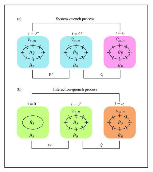
Figure 1: Quench processes. (a) A system-quench process begins with a Gibbs state relative to the Hamiltonian $\hat{H}_{S\cup R}=\hat{H}_{S}^{{A}}+\hat{H}_{R}+\hat{V}_{{S\cup R}}$. The system’s Hamiltonian is quenched to $\hat{H}_{S}^{{B}}$ at $t=0$. ${S\cup R}$ then evolves until time $t_{\rm f}$. (b) An interaction-quench process begins with a separable Gibbs state relative to the Hamiltonian $\hat{H}_{{S\cup R}}=\hat{H}_{S}+\hat{H}_{R}$. The interaction, $\hat{V}_{S\cup R}$, is turned on at $t=0$. In both processes, the quench injects work $W$ into the system. The system absorbs heat $Q$ during the subsequent evolution. A colored box represents ${S\cup R}$, and a black ellipse encloses $S$. Identical colors represent identical states. Squiggly lines indicate the interaction, $\hat{V}_{{S\cup R}}$.

System-quench process
Time	$\hat{H}_{{S\cup R}}(t)$	$\hat{\rho}_{S}(t)$
$t=0^{-}$	$\hat{H}_{S}^{A}+\hat{H}_{R}+\hat{V}_{{S\cup R}}$	$\hat{\pi}_{S}^{A}$
$t=0^{+}$	$\hat{H}_{S}^{B}+\hat{H}_{R}+\hat{V}_{{S\cup R}}$	$\hat{\pi}_{S}^{A}$
$t=t_{\rm f}$	$\hat{H}_{S}^{B}+\hat{H}_{R}+\hat{V}_{{S\cup R}}$	$\hat{\rho}_{S}(t_{\rm f})$
Interaction-quench process
Time	$\hat{H}_{{S\cup R}}(t)$	$\hat{\rho}_{S}(t)$
$t=0^{-}$	$\hat{H}_{S}+\hat{H}_{R}$	$\hat{\pi}_{S}^{A}=\hat{\pi}_{S}^{0}$
$t=0^{+}$	$\hat{H}_{S}+\hat{H}_{R}+\hat{V}_{{S\cup R}}$	$\hat{\pi}_{S}^{A}=\hat{\pi}_{S}^{0}$
$t=t_{\rm f}$	$\hat{H}_{S}+\hat{H}_{R}+\hat{V}_{{S\cup R}}$	$\hat{\rho}_{S}(t_{\rm f})$

Table 1: Overview of system- and interaction-quench processes.

These processes involve the following states. The global Gibbs state, relative to the Hamiltonian $\hat{H}_{{S\cup R}}^{\lambda}$, is $\hat{\pi}_{{S\cup R}}^{\lambda}$. The system’s corresponding equilibrium state is

$$\hat{\pi}_{S}^{\lambda}\coloneqq{\mathrm{Tr}}_{R}(\hat{\pi}_{{S\cup R}}^{\lambda})\equiv\frac{e^{-\beta\hat{H}_{S}^{*\lambda}}}{Z_{S}^{*\lambda}}\,.$$ (16)

At time $t$, ${S\cup R}$ and $S$ are in the states $\hat{\rho}_{{S\cup R}}(t)$ and $\hat{\rho}_{S}(t)$, respectively. By assumption, ${S\cup R}$ begins in equilibrium: $\hat{\rho}_{{S\cup R}}(0^{-})=\hat{\pi}_{{S\cup R}}^{{A}}$. In the interaction quench, $\hat{\pi}_{{S\cup R}}^{{A}}=\hat{\pi}_{S}^{0}\otimes\hat{\pi}_{R}^{0}$, wherein Eq.˜5 specifies $\hat{\pi}_{S}^{0}$ and $\hat{\pi}_{R}^{0}$. The state of ${S\cup R}$ does not change during either quench, by the sudden approximation :

$$\hat{\rho}_{S}(0^{+})=\hat{\rho}_{S}(0^{-})=\hat{\pi}_{S}^{A}\,.$$ (17)

From $t=0^{+}$ to $t_{\mathrm{f}}$, ${S\cup R}$ evolves under a fixed Hamiltonian: $\hat{H}_{S\cup R}(t)=\hat{H}_{{S\cup R}}^{{B}}$. We discuss this evolution at the end of Sec.˜V.

V Work, heat, and the second law

We now identify the work $W$ performed on, and the heat $Q$ absorbed by, the system during a quench process. The three internal-energy definitions (Sec.˜III) imply corresponding definitions of work and heat. As in classical contexts [75, 51, 45, 44], we determine which definitions satisfy the first and second laws of thermodynamics.

$U_{S}(t)$ denotes the system’s internal energy at time $t$, wherein $U_{S}$ denotes one of the candidate definitions: $U_{\mathrm{diff}}$, $U_{H*}$, or $U_{E^{*}}$. During a quench process, the system’s internal energy changes by an amount

$$\Delta U_{S}\coloneqq U_{S}\left(t_{\rm{f}}\right)-U_{S}\left(0^{-}\right)\,.$$ (18)

The first law of thermodynamics attributes the energy change to work and heat:

$$\Delta U_{S}=W+Q\,.$$ (19)

During the quench, no energy flows between the system and the reservoir, as neither subsystem’s state changes. Consequently, $S$ absorbs no heat; any change in the system’s internal energy (due to the sudden change in the Hamiltonian) is interpreted as work:

$$W\coloneqq U_{S}\left(0^{+}\right)-U_{S}\left(0^{-}\right)\,.$$ (20)

After the quench (from $t=0^{+}$ to $t_{\rm{f}}$), the state $\hat{\rho}_{S\cup R}$ evolves under a fixed Hamiltonian, $\hat{H}_{{S\cup R}}^{{B}}$. The energy transferred between $S$ and $R$ is interpreted as heat [58, 76]:

$$Q\coloneqq U_{S}\left(t_{\rm{f}}\right)-U_{S}\left(0^{+}\right)\,.$$ (21)

Equations˜20 and 21 satisfy the first law [Eq.˜19] by construction. They are motivated by the standard definitions used in weak-coupling quantum thermodynamics [77, 23, 76].

Different choices for $U_{S}$ in Eqs.˜20 and 21—$U_{\mathrm{diff}}$, $U_{H^{*}}$, and $U_{E^{*}}$—lead to different expressions for the work performed on $S$:

$$W_{\mathrm{diff}}\coloneqq{\mathrm{Tr}}_{SR}\left(\left[\hat{H}_{{S\cup R}}^{B}-\hat{H}_{{S\cup R}}^{A}\right]\;\hat{\pi}_{{S\cup R}}^{A}\right)\,,$$ (22)

$$W_{H^{*}}\coloneqq{\mathrm{Tr}}_{S}\left(\left[\hat{H}_{S}^{*B}-\hat{H}_{S}^{*A}\right]\;\pi_{S}^{A}\right)\,,$$ (23)

and

$$W_{E^{*}}\coloneqq{\mathrm{Tr}}_{S}\left(\left[\hat{E}_{S}^{*B}-\hat{E}_{S}^{*A}\right]\;\hat{\pi}_{S}^{A}\right)\,.$$ (24)

Similarly, different $U_{S}$ definitions yield different definitions for the heat absorbed by $S$:

$$Q_{\mathrm{diff}}\coloneqq{\mathrm{Tr}}_{SR}\left(\hat{H}_{{S\cup R}}^{B}\left[\hat{\rho}_{{S\cup R}}(t_{\rm f})-\hat{\pi}_{{S\cup R}}^{A}\right]\right)\,,$$ (25)

$$Q_{H^{*}}\coloneqq{\mathrm{Tr}}_{S}\left(\hat{H}_{S}^{*B}\left[\hat{\rho}_{S}(t_{\rm f})-\hat{\pi}_{S}^{A}\right]\right)\,,$$ (26)

and

$$Q_{E^{*}}\coloneqq{\mathrm{Tr}}_{S}\left(\hat{E}_{S}^{*B}\left[\hat{\rho}_{S}(t_{\rm f})-\hat{\pi}_{S}^{A}\right]\right)\,.$$ (27)

To state the second law, we introduce further notation. Denote by $F_{S}^{{A}}\coloneqq-\beta^{-1}\ln Z_{S}^{A*}$ the free energy of $S$ in the equilibrium state relative to the initial Hamiltonian. Define $F_{S}^{{B}}$ analogously relative to the final Hamiltonian. Because $S$ begins in the equilibrium state $\hat{\pi}_{S}^{{A}}$, the second law of thermodynamics assumes the form 

$$W\geq\Delta F_{S}\,,$$ (28)

wherein $\Delta F_{S}\coloneqq F_{S}^{{B}}-F_{S}^{{A}}$. In classical thermodynamics, Eq.˜28 is the statement of the second law for a system in contact with one thermal reservoir [42]. Equation˜28 remains valid even under strong system-reservoir coupling [44, 45], and even if $S$ does not end in equilibrium [57]. Rearranging Eq.˜28 yields $W-\Delta F_{S}\geq 0$. The greater the dissipated work $W-\Delta F_{S}$, the more irreversible the process [58].

We now show that two work definitions [Eqs.˜22 and 23] satisfy the second law. In each case, we calculate $W-\Delta F_{S}$ and prove the inequality in Eq.˜28. First consider $W_{\mathrm{diff}}$:

$$\beta\left(W_{\mathrm{diff}}-\Delta F_{S}\right) =\beta\left\{{\mathrm{Tr}}_{SR}\left(\left[\hat{H}_{{S\cup R}}^{{B}}-\hat{H}_{{S\cup R}}^{{A}}\right]\hat{\pi}_{{S\cup R}}^{{A}}\right)-\left(F_{S}^{{B}}-F_{S}^{{A}}\right)\right\}$$ (29a)

$$={\mathrm{Tr}}_{SR}\left(\left\{\beta\left[\hat{H}_{{S\cup R}}^{{B}}-F_{{S\cup R}}^{{B}}\right]-\beta\left[\hat{H}_{{S\cup R}}^{{A}}-F_{{S\cup R}}^{{A}}\right]\;\right\}\hat{\pi}_{{S\cup R}}^{A}\right)$$ (29b)

$$={\mathrm{Tr}}_{SR}\left(\left[\ln\hat{\pi}_{{S\cup R}}^{{A}}-\ln\hat{\pi}_{{S\cup R}}^{{B}}\right]\;\hat{\pi}_{{S\cup R}}^{{A}}\right)\geq 0\,.$$ (29c)

Equation˜29b follows from $F_{{S\cup R}}=F_{S}+F_{R}$ [from below Eqs.˜6, 7, and 8] and from ${\mathrm{Tr}}_{SR}(\hat{\pi}^{A/B}_{S\cup R})=1$; the equality in Eq.˜29c, from $\hat{\pi}_{{S\cup R}}=e^{-\beta\left(\hat{H}_{{S\cup R}}-F_{{S\cup R}}\right)}$; and the inequality, from the quantum relative entropy’s non-negativity . Similarly, for $W_{H^{*}}$,

$$\beta\left(W_{H^{*}}-\Delta F_{S}\right) =\beta\left\{{\mathrm{Tr}}_{S}\left(\left[\hat{H}_{S}^{*B}-\hat{H}_{S}^{*A}\right]\;\hat{\pi}_{S}^{{A}}\right)-\left(F_{S}^{{B}}-F_{S}^{{A}}\right)\right\}$$ (30a)

$$={\mathrm{Tr}}_{S}\left(\left\{\beta\left[\hat{H}_{S}^{*B}-F_{S}^{{B}}\right]-\beta\left[\hat{H}_{S}^{*A}-F_{S}^{{A}}\right]\right\}\;\hat{\pi}_{S}^{{A}}\right)$$ (30b)

$$={\mathrm{Tr}}_{S}\left(\left[\ln\hat{\pi}_{S}^{{A}}-\ln\hat{\pi}_{S}^{{B}}\right]\;\hat{\pi}_{S}^{{A}}\right)\geq 0\,.$$ (30c)

The equality in Eq.˜30c follows from $\hat{\pi}_{S}=e^{-\beta(\hat{H}_{S}^{*}-F_{S})}$. We lack an analogous derivation for $W_{E^{*}}$, and Sec.˜VI illustrates numerically that $W_{E*}$ can violate Eq.˜28. Thus, of the three quantum work definitions, only $W_{\mathrm{diff}}$ and $W_{H^{*}}$ satisfy the second law for our quench processes.

The values of $W_{\mathrm{diff}}$, $W_{H^{*}}$, and $W_{E^{*}}$ can differ. For system quenches, however, we show in Appendix˜C that, if

$$\left[\hat{H}_{S}^{A},\hat{V}_{{S\cup R}}\right]=\left[\hat{H}_{S}^{B},\hat{V}_{{S\cup R}}\right]=0\,,$$ (31)

then

$$W_{\mathrm{diff}}=W_{H^{*}}=W_{E^{*}}\,.$$ (32)

For classical systems undergoing system quenches, $W_{\mathrm{diff}}$, $W_{H^{*}}$, and $W_{E^{*}}$ are identical [44, 45].

If the system begins and ends in equilibrium, one can express the second law in terms of heat and entropy. Define the (thermal) entropy of an equilibrium state $\hat{\pi}_{S}$ [Eq.˜3] using the thermodynamic relation

$$\mathcal{S}\coloneq\beta(U_{S}-F_{S})\,.$$ (33)

$U_{S}$ evaluates to $U_{\mathrm{diff}}$, $U_{H^{*}}$, or $U_{E^{*}}$; and Eq.˜7 specifies $F_{S}$. Suppose $S$ ends in an equilibrium state at inverse temperature $\beta$,

$$\hat{\rho}_{S}(t_{\mathrm{f}})=\hat{\pi}_{S}^{{B}}\,.$$ (34)

Equation˜33, with the first law [Eq.˜19], implies that $W-\Delta F_{S}=\beta^{-1}\Delta\mathcal{S}-Q$. Hence the second law [Eq.˜28] is equivalent to

$$Q\leq\beta^{-1}\Delta\mathcal{S}\,.$$ (35)

Since Eqs.˜28 and 35 are equivalent when $S$ ends in equilibrium, Eqs.˜29 and 30 imply

$$Q_{\mathrm{diff}}\leq\beta^{-1}\Delta\mathcal{S}_{\mathrm{diff}}\,$$ (36)

and

$$Q_{H^{*}}\leq\beta^{-1}\Delta\mathcal{S}_{H^{*}}\,,$$ (37)

respectively. We show numerically in Sec.˜VI that $Q_{E^{*}}$ can violate Eq.˜35.

We derived Eqs.˜36 and 37 by assuming that $S$ ends in the equilibrium state $\hat{\pi}_{S}^{{B}}$ [Eq.˜34]. At least two realistic scenarios motivate this assumption:

1. Suppose that ${S\cup R}$ is a closed quantum system evolving unitarily under $\hat{H}_{{S\cup R}}^{{B}}$. Let ${S\cup R}$ satisfy the eigenstate thermalization hypothesis [80], and let $R$ have a thermal reservoir’s generic properties: macroscopically many DOFs and a heat capacity much greater than the system’s. For sufficiently large $t_{\mathrm{f}}$, one expects ${S\cup R}$ to equilibrate to a temperature essentially identical to the initial temperature, $\beta^{-1}$. In this case, $S$ ends in the state $\hat{\pi}_{S}^{{B}}$.

2. Suppose that ${S\cup R}$ couples weakly to a much larger, thermal super-reservoir at a temperature $\beta^{-1}$. If $t_{\mathrm{f}}$ is sufficiently large, then ${S\cup R}$ relaxes to the global Gibbs state $\hat{\pi}_{S\cup R}^{B}$, which implies Eq.˜34.

VI Two-spin model

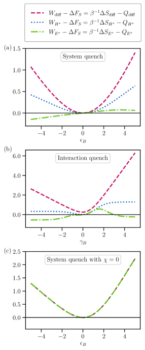
Figure 2: Thermodynamic quantities of the two-spin model. (a) During a system quench, the $\epsilon$ in Eq.˜38 changes from $\epsilon_{{A}}=0$ to $\epsilon_{{B}}$. The dissipated work is plotted as a function of $\epsilon_{{B}}$, with $\alpha=0.8$, $\gamma=1.2$, and $\chi=1.8$. $W_{\mathrm{diff}}$ and $W_{H^{*}}$ satisfy the second law [Eq.˜28]; consequently, so do $Q_{\mathrm{diff}}$ and $Q_{H^{*}}$ [Eq.˜35]. $W_{E^{*}}$ and $Q_{E^{*}}$ do not. (b) During an interaction quench, the coupling constants $\gamma$ and $\chi$ change from $\gamma_{A}=\chi_{A}=0$ to $\gamma_{B}$ and $\chi_{B}$. Dissipated work is plotted as a function of $\gamma_{B}$, with $\epsilon=1.0$, $\alpha=5.0$, and $\chi_{B}=1.2$. Qualitatively similar results follow from plotting the dissipated work as a function of $\chi_{B}$ at fixed $\epsilon$, $\alpha$, and $\gamma_{B}$. (c) We set $\chi=0$ in Eq.˜38, such that $\hat{H}_{S}$ commutes with $\hat{V}_{{S\cup R}}$ before and after the quench [Eq.˜31]. The work dissipated during a system quench is plotted as a function of $\epsilon_{{B}}$, with fixed $\epsilon_{{A}}=0$, $\alpha=0.8$, and $\gamma=1.2$. The three curves coincide, as expected [Eq.˜32].

A simple, illustrative model features spins $S$ and $R$. Denote by $\sigma_{a}^{i}$ the Pauli operator with $a\in\{S,R\}$ and $i\in\{x,z\}$. The spins evolve under the Hamiltonian

$$\hat{H}_{{S\cup R}}=\frac{\epsilon}{2}\sigma_{S}^{z}+\frac{\alpha}{2}\sigma_{R}^{z}+\gamma\sigma_{S}^{z}\sigma_{R}^{z}+\chi\sigma_{S}^{x}\sigma_{R}^{x}\,,$$ (38)

wherein $\gamma$ and $\chi$ denote coupling strengths. We assume ${S\cup R}$ couples weakly to a thermal super-reservoir at a temperature $\beta^{-1}$. Moreover, we assume $t_{\rm f}$ is sufficiently large for ${S\cup R}$ to equilibrate with the super-reservoir, postquench. (We do not model the super-reservoir explicitly.) These assumptions realize scenario (ii), sketched at the end of Sec.˜V. We compute the work, heat, free-energy change, and entropy change relevant to each quench described in Table˜1. Appendix˜D lists analytical expressions for these quantities. Here, we illustrate the conclusions of Sec.˜V by evaluating these expressions at specific $\epsilon$, $\alpha$, $\gamma$ and $\chi$ values. Throughout this section, $\beta=1$.

During a system quench, $\hat{H}_{S}\coloneqq\frac{\epsilon}{2}\,\sigma_{S}^{z}$ changes abruptly: $\epsilon$ switches from $\epsilon_{{A}}=0$ to $\epsilon_{{B}}$. $\alpha$, $\gamma$, and $\chi$ remain fixed. Figure˜2(a) displays the dissipated work, $W-\Delta F_{S}$, as a function of $\epsilon_{{B}}$. $W_{\mathrm{diff}}$ and $W_{H^{*}}$ satisfy the second law, in agreement with Eqs.˜29 and 30. In contrast, $W_{E^{*}}$ violates the second law at certain $\epsilon_{B}$ values.

During an interaction quench, $\gamma$ and $\chi$ change suddenly from $\gamma_{{A}}=\chi_{{A}}=0$ to $\gamma_{{B}}$ and $\chi_{{B}}$. Figure˜2(b) displays the dissipated work as a function of $\gamma_{B}$. The other parameters remain fixed. Again, $W_{\mathrm{diff}}$ and $W_{H^{*}}$ satisfy the second law. However, $W_{E^{*}}$ violates it at some $\gamma_{B}$ values.

Turning to Fig.˜2(c), we return to the system quench. However, we now set $\chi=0$ in Eq.˜38, to satisfy the commutation relations in Eq.˜31. In agreement with Eq.˜32, the three dissipated-work quantities equal each other. Additionally, they obey the second law.

Strong-coupling quantum thermodynamics naturally applies to lattice gauge theories, as proposed in Ref. [81]. Gauge theories and their lattice formulations are crucial to high-energy and nuclear physics [82, 83], condensed and synthetic quantum matter [84, 85, 86, 87], and quantum information science [88, 89, 90, 91, 92, 93, 94, 95]. Local constraints among DOFs define lattice gauge theories. Physical systems can only be in states consistent with those constraints. A slight modification converts our two-spin model into a simple lattice gauge theory. We introduce an LGT-type constraint by setting $k=-\gamma>0$ and adding a term $k\mathbbm{1}_{{S\cup R}}$ to $\hat{H}_{{S\cup R}}$ in Eq.˜38:

$$\hat{H}_{{S\cup R}}=\frac{\epsilon}{2}\sigma_{S}^{z}+\frac{\alpha}{2}\sigma_{R}^{z}+\chi\sigma_{S}^{x}\sigma_{R}^{x}+k(\mathbbm{1}_{{S\cup R}}-\sigma_{S}^{z}\sigma_{R}^{z})\,.$$ (39)

In the limit as $k\to\infty$ (at a fixed, finite temperature), the last term acts as an energy penalty: it constrains the system to the eigenvalue-1 eigenspace of $\sigma^{z}_{S}\sigma^{z}_{R}$. This operator serves as a Gauss-law operator. It specifies which states satisfy the constraint. Since the interactions in Eq.˜39 are non-negligible, strong-coupling quantum thermodynamics applies to this model, as to other lattice gauge theories [81].

VII Discussion and outlook

We have scrutinized definitions of thermodynamic properties of strongly coupled quantum systems. We compared three definitions of the system’s internal energy—$U_{\mathrm{diff}}$, $U_{H^{*}}$, and $U_{E^{*}}$ [Eqs.˜10, 11, and 13]—during quench processes. All three lead to work and heat definitions that satisfy the first law of thermodynamics, by construction. However, we found, only the definitions based on $U_{\mathrm{diff}}$ and $U_{H^{*}}$ satisfy the second law. These conclusions hold independently of the final states when the second law is expressed in terms of work and free energy. If the system equilibrates after the quench, the same conclusions hold when the second law is expressed in terms of heat and entropy. We illustrated these general results with a simple model of two coupled spins. These conclusions distinguish quantum from classical thermodynamics. Our work can therefore guide the thermodynamics of strongly coupled quantum systems of relevance to condensed matter, high-energy and nuclear physics, quantum chemistry, and quantum error correction (see, e.g., Refs. [96, 81, 97, 98]).

This work opens the door to further opportunities:

• We focused on quench processes because they allow for naturally partitioning the system’s internal-energy change into work and heat, even when the system and reservoir couple strongly. Our results may extend to thermodynamic processes beyond quenches, where the partitioning is less clear. Examples include quantum-adiabatic processes, used to prepare quantum states in quantum simulations, and particle collisions, relevant to hydrodynamics [99] and nuclear and high-energy physics [81, 100, 101].

• In this work, we have defined average work and heat quantities. One can define classical work and heat as fluctuating quantities, whose values differ from realization to realization of a process. Fluctuation theorems (extensions of the second law), derived in this setting [75, 102, 51, 57, 45, 103, 104, 105, 52, 44, 106, 107], have been extended to strong system-reservoir couplings [51, 44, 45, 52]. Can one define fluctuating work and heat exchanged within strongly coupled quantum systems? For example, the two-point-measurement definition of work supports a fluctuation theorem for closed quantum systems [8, 9, 10, 55, 108, 25, 109]. One can apply this scheme in strong-coupling contexts by treating ${S\cup R}$ as a closed quantum system. Yet can one infer the fluctuating work performed on $S$ from measurements of $S$ alone?

• Of the two internal-energy definitions that obey the second law, one [Eq.˜11] stems from the Hamiltonian of mean force, $\hat{H}_{S}^{*}$ [Eq.˜4]. This operator is related to the system’s entanglement Hamiltonian if ${S\cup R}$ is in equilibrium [81]. Entanglement-Hamiltonian tomography enables efficient experimental measurements, or numerical determinations, of a subsystem’s quantum state [110, 111, 112, 113, 114]. Such tomography has been applied to ground, excited, and nonequilibrium states of isolated systems [115, 116, 117, 118, 59, 119, 120, 121]. Future work will extend entanglement-Hamiltonian tomography to thermal states. This extension will allow one to access thermodynamic quantities in the strong-coupling regime of quantum simulations.

VIII Acknowledgments

We thank Sherry Wang for valuable feedback on the manuscript. Z. D., G. O., and C. P. were supported by the National Science Foundation (NSF) Quantum Leap Challenge Institutes (QLCI) (award no. OMA-2120757). Z. D. further acknowledges funding by the Department of Energy (DOE), Office of Science, Early Career Award (award no. DESC0020271), as well as by the Department of Physics; Maryland Center for Fundamental Physics; and College of Computer, Mathematical, and Natural Sciences at the University of Maryland, College Park. She is grateful for the hospitality of Perimeter Institute, and of Kavli Institute for Theoretical Physics (KITP), where part of this work was carried out. Research at Perimeter Institute is supported in part by the Government of Canada through the Department of Innovation, Science, and Economic Development and by the Province of Ontario through the Ministry of Colleges and Universities. Z. D. was also supported in part by the Simons Foundation through the Simons Foundation Emmy Noether Fellows Program at Perimeter Institute. Research at the KITP was supported in part by the NSF award PHY-2309135. C. J. and N. Y. H. further acknowledge support from John Templeton Foundation (award no. 62422). N. Y. H. thanks Harry Miller for conversations about strong-coupling thermodynamics. N. M. acknowledges funding by the DOE, Office of Science, Office of Nuclear Physics, IQuS (https://iqus.uw.edu), via the program on Quantum Horizons: QIS Research and Innovation for Nuclear Science under Award DE-SC0020970. C. P. is grateful for discussions about thermal gauge theories with Robert Pisarski and for the hospitality of Brookhaven National Laboratory, which hosted C. P. as part of an Office of Science Graduate Student Research Fellowship. G. O. further acknowledges support from the American Association of University Women through an International Fellowship. Finally, N. M., G. O., C. P., and N. Y. H. thank the participants of the InQubator for Quantum Simulation (IQuS) workshop “Thermalization, from Cold Atoms to Hot Quantum Chromodynamics,” which took place at the University of Washington in September 2023, for valuable discussions.

Appendix A Weak-coupling limit

In the weak-coupling limit, the interactions between $S$ and $R$, while nonvanishing, are small enough to be neglected in calculations of partition functions and free energies. Therefore, we model the weak-coupling limit by setting $V_{{S\cup R}}=0$ in Eq.˜1:

$$\hat{H}_{{S\cup R}}=\hat{H}_{S}+\hat{H}_{R}\,.$$ (40)

In this limit, we demonstrate, the main text’s three internal-energy definitions are equivalent.

Under the assumption in Eq.˜40, one obtains

$$\hat{H}_{S}^{*}\coloneqq-\frac{1}{\beta}\ln{\left(\frac{{\mathrm{Tr}}_{R}\left(e^{-\beta\left(\hat{H}_{S}+\hat{H}_{R}\right)}\right)}{{\mathrm{Tr}}_{R}\left(e^{-\beta\hat{H}_{R}}\right)}\right)}=-\frac{1}{\beta}\ln{\left(e^{-\beta\hat{H}_{S}}\right)}=\hat{H}_{S}\,$$ (41)

and

$$\hat{E}_{S}^{*}\coloneqq\partial_{\beta}\left(\beta\hat{H}_{S}^{*}\right)=\partial_{\beta}\left(\beta\hat{H}_{S}\right)=\hat{H}_{S}\,.$$ (42)

Thus, both $\hat{H}_{S}^{*}$ and $\hat{E}_{S}^{*}$ reduce to the system Hamiltonian $\hat{H}_{S}$ in the weak-coupling limit. Consequently, by Eqs.˜11 and 13,

$$U_{H^{*}}=U_{E^{*}}={\mathrm{Tr}}_{S}\left(\hat{H}_{S}\;\hat{\rho}_{S}\right)\,,$$ (43)

for any state $\hat{\rho}_{S}$.

We now additionally assume that ${S\cup R}$ is in a global Gibbs state. As a result, $\hat{\rho}_{S}=\hat{\pi}_{S}^{0}$, $U_{H^{*}}=U_{E^{*}}=U_{S}^{0}$, and

$$U_{\mathrm{diff}} ={\mathrm{Tr}}_{SR}\left(\left[\hat{H}_{S}\otimes\hat{\mathbbm{1}}_{R}+\hat{\mathbbm{1}}_{S}\otimes\hat{H}_{R}\right]\left[\hat{\pi}_{S}^{0}\otimes\hat{\pi}_{R}^{0}\right]\right)-{\mathrm{Tr}}_{R}\left(\hat{H}_{R}\;\hat{\pi}_{R}^{0}\right)$$ (44a)

$$={\mathrm{Tr}}_{S}\left(\hat{H}_{S}\;\hat{\pi}_{S}^{0}\right)+{\mathrm{Tr}}_{R}\left(\hat{H}_{R}\;\hat{\pi}_{R}^{0}\right)-{\mathrm{Tr}}_{R}\left(\hat{H}_{R}\;\hat{\pi}_{R}^{0}\right)$$ (44b)

$$={\mathrm{Tr}}_{S}\left(\hat{H}_{S}\;\hat{\pi}_{S}^{0}\right)=U_{S}^{0}\,.$$ (44c)

Thus,

$$U_{\mathrm{diff}}=U_{H^{*}}=U_{E^{*}}=U_{S}^{0}\,.$$ (45)

Three internal-energy definitions would be equivalent in the weak-coupling limit if one defined $U_{\mathrm{diff}}$ differently from Eq.˜10. Define $U_{R}\coloneqq{\mathrm{Tr}}_{R}(\hat{H}_{R}\rho_{R})$ and $\widetilde{U}_{\mathrm{diff}}\coloneqq U_{{S\cup R}}-U_{R}$. If $\rho_{{S\cup R}}$ is any product state $\rho_{S}\otimes\rho_{R}$, then $\widetilde{U}_{\mathrm{diff}}=U_{H^{*}}=U_{E^{*}}$. Since $\widetilde{U}_{\mathrm{diff}}$ is nonstandard, we use Eq.˜10 in this manuscript.

Appendix B Equivalence of $U_{\mathrm{diff}}$ and $U_{E^{*}}$ when $S\cup R$ is in a global Gibbs state

In this appendix, we show that $U_{E^{*}}=U_{\mathrm{diff}}$ when ${S\cup R}$ is in a global Gibbs state. The classical analogue was proved in Ref. [44], then used in Ref. [46] to derive quantum fluctuation theorems. We do not assume, in this appendix, that the coupling is weak.

We begin by rewriting Eq.˜12:

$$\hat{E}_{S}^{*} =\partial_{\beta}\left(\beta\hat{H}_{S}^{*}\right)$$ (46a)

$$=\partial_{\beta}\left[-\ln{\left(\frac{{\mathrm{Tr}}_{R}\left(e^{-\beta\hat{H}_{{S\cup R}}}\right)}{{\mathrm{Tr}}_{R}\left(e^{-\beta\hat{H}_{R}}\right)}\right)}\;\right]$$ (46b)

$$=-\frac{\partial_{\beta}\left[{\mathrm{Tr}}_{R}\left(e^{-\beta\hat{H}_{{S\cup R}}}\right)\right]}{{\mathrm{Tr}}_{R}\left(e^{-\beta\hat{H}_{{S\cup R}}}\right)}+\frac{\partial_{\beta}\left[{\mathrm{Tr}}_{R}\left(e^{-\beta\hat{H}_{R}}\right)\right]}{{\mathrm{Tr}}_{R}\left(e^{-\beta\hat{H}_{R}}\right)}\,.$$ (46c)

Consider applying the derivative’s definition to the first term:

$$\partial_{\beta}\left[{\mathrm{Tr}}_{R}\left(e^{-\beta\hat{H}_{{S\cup R}}}\right)\right] =\lim_{\delta\beta\to 0}\frac{{\mathrm{Tr}}_{R}\left(e^{-\left(\beta+\delta\beta\right)\hat{H}_{{S\cup R}}}\right)-{\mathrm{Tr}}_{R}\left(e^{-\beta\hat{H}_{{S\cup R}}}\right)}{\delta\beta}$$ (47a)

$$=\lim_{\delta\beta\to 0}{\mathrm{Tr}}_{R}\left(e^{-\beta\hat{H}_{{S\cup R}}}\frac{\left(e^{-\delta\beta\hat{H}_{{S\cup R}}}-1\right)}{\delta\beta}\right)$$ (47b)

$$=-{\mathrm{Tr}}_{R}\left(\hat{H}_{{S\cup R}}\;e^{-\beta\hat{H}_{{S\cup R}}}\right)\,.$$ (47c)

The final term in Eq.˜46 simplifies similarly. Therefore,

$$\hat{E}_{S}^{*}=\frac{{\mathrm{Tr}}_{R}\left(\hat{H}_{{S\cup R}}\;e^{-\beta\hat{H}_{{S\cup R}}}\right)}{{\mathrm{Tr}}_{R}\left(e^{-\beta\hat{H}_{{S\cup R}}}\right)}-\frac{{\mathrm{Tr}}_{R}\left(\hat{H}_{R}\;e^{-\beta\hat{H}_{R}}\right)}{{\mathrm{Tr}}_{R}\left(e^{-\beta\hat{H}_{R}}\right)}\,.$$ (48)

To calculate $U_{E^{*}}$, one takes the expectation value of $\hat{E}_{S}^{*}$ in the state $\hat{\pi}_{S}$:

$$U_{E^{*}}={\mathrm{Tr}}_{S}\left(\hat{E}_{S}^{*}\;\hat{\pi}_{S}\right)\,.$$ (49)

Substituting $\hat{\pi}_{S}={\mathrm{Tr}}_{R}\left(\hat{\pi}_{{S\cup R}}\right)$, and $\hat{E}^{*}_{S}$ from Eq.˜48, gives

$$U_{E^{*}}=\frac{1}{Z_{{S\cup R}}}{\mathrm{Tr}}_{S}\bm{\big{(}}{\mathrm{Tr}}_{R}\big{(}\hat{H}_{{S\cup R}}\;e^{-\beta\hat{H}_{{S\cup R}}}\big{)}\bm{\big{)}}-\frac{1}{Z_{R}}{\mathrm{Tr}}_{S}\bm{\big{(}}\hat{\pi}_{S}\;{\mathrm{Tr}}_{R}\big{(}\hat{H}_{R}e^{-\beta\hat{H}_{R}}\big{)}\bm{\big{)}}\,.$$ (50)

By distributing and evaluating the traces, one obtains

$$U_{E^{*}} ={\mathrm{Tr}}_{SR}\left(\hat{H}_{{S\cup R}}\;\hat{\pi}_{{S\cup R}}\right)-{\mathrm{Tr}}_{S}\left(\hat{\pi}_{S}\right){\mathrm{Tr}}_{R}\left(\hat{H}_{R}\;\hat{\pi}_{R}\right)$$ (51a)

$$={\mathrm{Tr}}_{SR}\left(\hat{H}_{{S\cup R}}\;\hat{\pi}_{{S\cup R}}\right)-U_{R}^{0}\,.$$ (51b)

Therefore, when $\hat{\rho}_{S\cup R}=\hat{\pi}_{S\cup R}$,

$$U_{E^{*}}=U_{\mathrm{diff}}\,.$$ (52)

Appendix C Operator commutativity and equal work quantities in a system quench

We show here that, if the commutation relations in Eq.˜31 hold, then $W_{\mathrm{diff}}=W_{H^{*}}=W_{E^{*}}$ during a system quench. One should expect this result for two reasons: the corresponding classical work definitions are equivalent for a system quench (although heat definitions are not) [45], and classical observables commute.

Recall that a system-quench process proceeds as follows. ${S\cup R}$ begins in the Gibbs state $\hat{\pi}_{{S\cup R}}^{{A}}$ at $t=0^{-}$. At $t=0$, one quenches the system Hamiltonian from $\hat{H}_{S}^{{A}}$ to $\hat{H}_{S}^{{B}}$. From $t=0^{+}$ to $t_{\mathrm{f}}$, ${S\cup R}$ evolves under $\hat{H}_{S\cup R}^{{B}}$.

First, we show that $W_{\mathrm{diff}}=W_{H^{*}}$ if the commutation relations (31) hold. Substituting the $\hat{H}_{S}^{*}$ definition [Eq.˜4] into the $W_{H^{*}}$ definition [Eq.˜23], one obtains

$$W_{H^{*}}=-\frac{1}{\beta}{\mathrm{Tr}}_{S}\bm{\Big{(}}\ln{\left({\mathrm{Tr}}_{R}\left(e^{-\beta\hat{H}_{{S\cup R}}^{{B}}}\right)\right)}\hat{\pi}_{S}^{{A}}\bm{\Big{)}}+\frac{1}{\beta}{\mathrm{Tr}}_{S}\bm{\Big{(}}\ln{\left({\mathrm{Tr}}_{R}\left(e^{-\beta\hat{H}_{{S\cup R}}^{{A}}}\right)\right)}\hat{\pi}_{S}^{{A}}\bm{\Big{)}}\,.$$ (53)

The expression simplifies because $\hat{H}_{S}^{{A}}$ and $\hat{H}_{S}^{{B}}$ commute with $\hat{V}_{{S\cup R}}$:

$$W_{H^{*}}= -\frac{1}{\beta}{\mathrm{Tr}}_{S}\bm{\Big{(}}\ln{\left(e^{-\beta\hat{H}_{S}^{B}}{\mathrm{Tr}}_{R}\left(e^{-\beta(\hat{H}_{R}+\hat{V}_{{S\cup R}})}\right)\right)}\hat{\pi}_{S}^{{A}}\bm{\Big{)}}+\frac{1}{\beta}{\mathrm{Tr}}_{S}\bm{\Big{(}}\ln{\left(e^{-\beta\hat{H}_{S}^{A}}{\mathrm{Tr}}_{R}\left(e^{-\beta(\hat{H}_{R}+\hat{V}_{{S\cup R}})}\right)\right)}\hat{\pi}_{S}^{{A}}\bm{\Big{)}}$$ (54a)

$$= -\frac{1}{\beta}{\mathrm{Tr}}_{S}\bm{\Big{(}}\ln{\left(e^{-\beta\hat{H}_{S}^{B}}\right)}\hat{\pi}_{S}^{{A}}\bm{\Big{)}}+\frac{1}{\beta}{\mathrm{Tr}}_{S}\bm{\Big{(}}\ln{\left(e^{-\beta\hat{H}_{S}^{A}}\right)}\hat{\pi}_{S}^{{A}}\bm{\Big{)}}\,.$$ (54b)

We substitute $\hat{\pi}_{S}^{{A}}={\mathrm{Tr}}_{R}(\hat{\pi}_{{S\cup R}}^{{A}})$, rearrange the traces, and recall that $\hat{H}_{S}^{{B}}-\hat{H}_{S}^{{A}}=\hat{H}_{{S\cup R}}^{{B}}-\hat{H}_{{S\cup R}}^{{A}}$:

$$W_{H^{*}}={\mathrm{Tr}}_{SR}\left(\left[\hat{H}_{{S\cup R}}^{{B}}-\hat{H}_{{S\cup R}}^{{A}}\right]\hat{\pi}_{{S\cup R}}^{{A}}\right)=W_{\mathrm{diff}}\,.$$ (55)

To obtain a similar expression for $W_{E^{*}}$, we apply the definitions of $\hat{H}_{S}^{*}$ [Eq.˜4] and $\hat{E}_{S}^{*}$ [Eq.˜12], as well as the commutation relations [Eq.˜31]. The difference $\hat{E}_{S}^{*B}-\hat{E}_{S}^{*A}$ becomes

$$\hat{E}_{S}^{*B}-\hat{E}_{S}^{*A} =\partial_{\beta}\left(\beta\hat{H}_{S}^{*B}-\beta\hat{H}_{S}^{*A}\right)$$ (56a)

$$=-\partial_{\beta}\left[\ln\bigg{(}{\mathrm{Tr}}_{R}\left(e^{-\beta\hat{H}_{{S\cup R}}^{{B}}}\right)\bigg{)}-\ln\bigg{(}{\mathrm{Tr}}_{R}\left(e^{-\beta\hat{H}_{{S\cup R}}^{{A}}}\right)\bigg{)}\right]$$ (56b)

$$=-\partial_{\beta}\Biggl{[}\ln\bigg{(}e^{-\beta\hat{H}_{S}^{B}}{\mathrm{Tr}}_{R}\left(e^{-\beta(\hat{H}_{R}+\hat{V}_{{S\cup R}})}\right)\bigg{)}-\ln\bigg{(}e^{-\beta\hat{H}_{S}^{A}}{\mathrm{Tr}}_{R}\left(e^{-\beta(\hat{H}_{R}+\hat{V}_{{S\cup R}})}\right)\bigg{)}\Biggl{]}$$ (56c)

$$=\hat{H}_{S}^{{B}}-\hat{H}_{S}^{{A}}\,.$$ (56d)

Inserting Eq.˜56d into Eq.˜24, with $\hat{\pi}_{S}^{A}={\mathrm{Tr}}_{R}\left(\hat{\pi}_{{S\cup R}}^{{A}}\right)$, gives

$$W_{E^{*}}={\mathrm{Tr}}_{SR}\left(\left[\hat{H}_{{S\cup R}}^{{B}}-\hat{H}_{{S\cup R}}^{{A}}\right]\hat{\pi}_{{S\cup R}}^{{A}}\right)=W_{\mathrm{diff}}\,.$$ (57)

Thus, $W_{\mathrm{diff}}=W_{H^{*}}=W_{E^{*}}$ when a system quench obeys the commutation relations (31). In contrast, even when the commutation relations hold, the three work quantities differ if the interaction term changes abruptly. We speculate that this observation extends to the analogous classical setup.

Appendix D Explicit expressions for work and heat exchanged in the two-spin model

We analytically derive expressions for the work, heat, entropy, and free energy in the two-spin model of Sec.˜VI. We use these expressions to generate Fig.˜2.

The spin Hamiltonian $\hat{H}_{{S\cup R}}$ [Eq.˜38] can be diagonalized easily. In terms of the eigenbasis of $\hat{H}_{{S\cup R}}$, the Gibbs state is

$$\hat{\pi}_{{S\cup R}}=\frac{1}{Z_{{S\cup R}}}\text{diag}\left(e^{-\beta(\gamma-\eta_{+})},e^{-\beta(\gamma+\eta_{+})},e^{\beta(\gamma+\eta_{-})},e^{\beta(\gamma-\eta_{-})}\right)\,.$$ (58)

We have defined $\eta_{\pm}\coloneqq\sqrt{{\left(\frac{\epsilon}{2}\pm\frac{\alpha}{2}\right)}^{2}+\chi^{2}}$, where $\epsilon$, $\alpha$, and $\chi$ are the Hamiltonian parameters. The partition function is

$$Z_{{S\cup R}}=2e^{-\beta\gamma}\cosh{\left(\beta\eta_{+}\right)}+2e^{\beta\gamma}\cosh{\left(\beta\eta_{-}\right)}\,.$$ (59)

To calculate the system’s thermal state, we trace out the reservoir from $\hat{\pi}_{{S\cup R}}$. In terms of the $\sigma_{S}^{z}$ eigenbasis,

$$\hat{\pi}_{S}=\frac{1}{Z_{{S\cup R}}}\begin{pmatrix}X_{-}&0\\ 0&X_{+}\end{pmatrix}\ ,$$ (60)

wherein

$$X_{\pm}=e^{-\beta\gamma}\left[\cosh{\left(\beta\eta_{+}\right)}\pm\frac{a_{+}}{\eta_{+}}\sinh{\left(\beta\eta_{+}\right)}\right]+e^{\beta\gamma}\left[\cosh{\left(\beta\eta_{-}\right)}\pm\frac{a_{-}}{\eta_{-}}\sinh{\left(\beta\eta_{-}\right)}\right]\,$$ (61)

and $a_{\pm}=(\epsilon\pm\alpha)/2$. Using the same basis, we also calculate $\hat{H}_{S}^{*}$ and $\hat{E}_{S}^{*}$:

$$\hat{H}_{S}^{*}=-\frac{1}{\beta}\begin{pmatrix}\ln{\left(\frac{X_{-}}{2\cosh{\left(\frac{\beta\alpha}{2}\right)}}\right)}&0\\ 0&\ln{\left(\frac{X_{+}}{2\cosh{\left(\frac{\beta\alpha}{2}\right)}}\right)}\end{pmatrix}\,,$$ (62)

and

$$\hat{E}_{S}^{*}=\begin{pmatrix}-\frac{\partial_{\beta}X_{-}}{X_{-}}+\frac{\alpha}{2}\tanh{\left(\frac{\beta\alpha}{2}\right)}&0\\ 0&-\frac{\partial_{\beta}X_{+}}{X_{+}}+\frac{\alpha}{2}\tanh{\left(\frac{\beta\alpha}{2}\right)}\end{pmatrix}\,.$$ (63)

D.1 System quench

During the system quench, the system-Hamiltonian parameter $\epsilon$ in Eq.˜38 changes from $\epsilon_{{A}}$ to $\epsilon_{B}$ [see Table˜1 and Fig.˜1(a)]. Let us define $a_{+}^{{A}}\coloneqq a_{+}\lvert_{\epsilon=\epsilon_{{A}}}$. We analogously define other quantities that carry ${A}$ or ${B}$ superscripts.

Equations˜22, 23, and 24 show the three work definitions. The first evaluates to

$$W_{\mathrm{diff}}=\frac{\left(\epsilon_{{A}}-\epsilon_{{B}}\right)}{Z_{{S\cup R}}^{{A}}}\left[\frac{a_{+}^{{A}}}{\eta_{+}^{{A}}}e^{-\beta\gamma}\sinh{\left(\beta\eta_{+}^{{A}}\right)}+\frac{a_{-}^{{A}}}{\eta_{-}^{{A}}}e^{\beta\gamma}\sinh{\left(\beta\eta_{-}^{{A}}\right)}\right]\,.$$ (64)

We substitute Eqs.˜60 and 62 into Eq.˜23, with superscripts $A$ and $B$ denoting the parameter values $\epsilon_{{A}}$ and $\epsilon_{{B}}$:

$$W_{H^{*}}=\frac{-1}{\beta Z_{{S\cup R}}^{{A}}}\left[X_{-}^{{A}}\ln{\left(\frac{X_{-}^{{B}}}{X_{-}^{{A}}}\right)}+X_{+}^{{A}}\ln{\left(\frac{X_{+}^{{B}}}{X_{+}^{{A}}}\right)}\right]\ .$$ (65)

Analogously, we calculate $W_{E^{*}}$ using Eqs.˜60, 63, and 24:

$$W_{E^{*}}=\frac{1}{Z_{{S\cup R}}^{{A}}}\Big{(}\partial_{\beta}X_{-}^{{A}}-\frac{X_{-}^{{A}}}{X_{-}^{{B}}}\partial_{\beta}X_{-}^{{B}}+\partial_{\beta}X_{+}^{{A}}-\frac{X_{+}^{{A}}}{X_{+}^{{B}}}\partial_{\beta}X_{+}^{{B}}\Big{)}\,.$$ (66)

One can calculate the heat similarly:

$$Q_{\mathrm{diff}} =\frac{1}{Z_{{S\cup R}}^{{B}}}\left\{2\gamma\left[e^{-\beta\gamma}\cosh{\left(\beta\eta_{+}^{{B}}\right)}-e^{\beta\gamma}\cosh{\left(\beta\eta_{-}^{{B}}\right)}\right]-2\eta_{+}^{{B}}e^{-\beta\gamma}\sinh{\left(\beta\eta_{+}^{{B}}\right)}-2\eta_{-}^{{B}}e^{\beta\gamma}\sinh{\left(\beta\eta_{-}^{{B}}\right)}\right\}$$

$$+\frac{1}{Z_{{S\cup R}}^{{A}}}\Big{\{}2\gamma\left[-e^{-\beta\gamma}\cosh{\left(\beta\eta_{+}^{{A}}\right)}+e^{\beta\gamma}\cosh{\left(\beta\eta_{-}^{{A}}\right)}\right]+2e^{-\beta\gamma}\sinh{\left(\beta\eta_{+}^{{A}}\right)}\left(\frac{a_{+}^{{B}}a_{+}^{{A}}+\chi^{2}}{\eta_{+}^{{A}}}\right)+2e^{\beta\gamma}\sinh{\left(\beta\eta_{-}^{{A}}\right)}\left(\frac{a_{-}^{{B}}a_{-}^{{A}}+\chi^{2}}{\eta_{-}^{{A}}}\right)\Big{\}}\,,$$ (67)

$$Q_{H^{*}}=\frac{1}{\beta}\Bigg{[}\left(\frac{X_{-}^{{A}}}{Z_{{S\cup R}}^{{A}}}-\frac{X_{-}^{{B}}}{Z_{{S\cup R}}^{{B}}}\right)\ln{X_{-}^{{B}}}+\left(\frac{X_{+}^{{A}}}{Z_{{S\cup R}}^{{A}}}-\frac{X_{+}^{{B}}}{Z_{{S\cup R}}^{{B}}}\right)\ln{X_{+}^{{B}}}\Bigg{]}\,,$$ (68)

and

$$Q_{E^{*}}=\left(\frac{X_{-}^{{A}}}{Z_{{S\cup R}}^{{A}}}-\frac{X_{-}^{{B}}}{Z_{{S\cup R}}^{{B}}}\right)\frac{\partial_{\beta}X_{-}^{{B}}}{X_{-}^{{B}}}+\left(\frac{X_{+}^{{A}}}{Z_{{S\cup R}}^{{A}}}-\frac{X_{+}^{{B}}}{Z_{{S\cup R}}^{{B}}}\right)\frac{\partial_{\beta}X_{+}^{{B}}}{X_{+}^{{B}}}\,.$$ (69)

During a system quench, the system’s free energy [Eq.˜7] changes by an amount

$$\Delta F_{S}=-\frac{1}{\beta}\ln{\left(\frac{e^{-\beta\gamma}\cosh{\left(\beta\eta_{+}^{{B}}\right)}+e^{\beta\gamma}\cosh{\left(\beta\eta_{-}^{{B}}\right)}}{e^{-\beta\gamma}\cosh{\left(\beta\eta_{+}^{{A}}\right)}+e^{\beta\gamma}\cosh{\left(\beta\eta_{-}^{{A}}\right)}}\right)}\,.$$ (70)

The three internal-energy definitions lead to three entropy definitions via Eq.˜33:

$$\Delta\mathcal{S}_{\mathrm{diff}}=\Delta\mathcal{S}_{E^{*}}=-\beta\Biggl{(}\frac{\partial_{\beta}X_{-}^{{B}}+\partial_{\beta}X_{+}^{{B}}}{Z_{{S\cup R}}^{{B}}}-\frac{\partial_{\beta}X_{-}^{{A}}+\partial_{\beta}X_{+}^{{A}}}{Z_{{S\cup R}}^{{A}}}\Biggr{)}+\ln{\left(\frac{Z_{{S\cup R}}^{{B}}}{Z_{{S\cup R}}^{{A}}}\right)}\,,$$ (71)

and

$$\Delta\mathcal{S}_{H^{*}}=\frac{X_{-}^{{B}}}{Z_{{S\cup R}}^{{B}}}\ln{\left(\frac{Z_{{S\cup R}}^{{B}}}{X_{-}^{{B}}}\right)}-\frac{X_{-}^{{A}}}{Z_{{S\cup R}}^{{A}}}\ln{\left(\frac{Z_{{S\cup R}}^{{A}}}{X_{-}^{{A}}}\right)}+\frac{X_{+}^{{B}}}{Z_{{S\cup R}}^{{B}}}\ln{\left(\frac{Z_{{S\cup R}}^{{B}}}{X_{+}^{{B}}}\right)}-\frac{X_{+}^{{A}}}{Z_{{S\cup R}}^{{A}}}\ln{\left(\frac{Z_{{S\cup R}}^{{A}}}{X_{+}^{{A}}}\right)}\,.$$ (72)

Since ${S\cup R}$ begins and ends in a Gibbs state, $\Delta U_{\mathrm{diff}}=\Delta U_{E^{*}}$ implies that $\Delta S_{\mathrm{diff}}=\Delta S_{E^{*}}$ [Eqs.˜33 and 52].

D.2 Interaction quench

During an interaction quench, the system-reservoir interaction changes abruptly [see Table˜1 and Fig.˜1(b)]. The coupling parameters, $\gamma$ and $\chi$, change from zero to $\gamma_{{B}}$ and $\chi_{{B}}$ at $t=0$. Subsequently, ${S\cup R}$ evolves to a Gibbs state of the Hamiltonian $\hat{H}_{S\cup R}^{B}$ [Eq.˜38]. The initial state $\hat{\pi}_{S}^{0}\otimes\hat{\pi}_{R}^{0}$ contains the factors

$$\hat{\pi}_{S}^{0}=\frac{1}{2\cosh{\left({\beta\epsilon}/{2}\right)}}\begin{pmatrix}\epsilon/2&0\\ 0&-\epsilon/2\end{pmatrix}\,$$ (73)

and

$$\hat{\pi}_{R}^{0}=\frac{1}{2\cosh{\left({\beta\alpha}/{2}\right)}}\begin{pmatrix}\alpha/2&0\\ 0&-\alpha/2\end{pmatrix}\,,$$ (74)

in terms of the $\sigma_{S}^{z}$ and $\sigma_{R}^{z}$ eigenbases, respectively. At $t=0^{-}$, $S$ and $R$ do not interact; hence $\gamma_{{A}}=\chi_{{A}}=0$, and $\hat{H}_{S}^{*A}=\hat{E}_{S}^{*A}=\hat{H}_{S}^{{A}}$ (see appendix˜A). When $t>0$, $\hat{H}_{S}^{*B}$ and $\hat{E}_{S}^{*B}$ have the forms in Eqs.˜62 and 63, with $\gamma_{{B}},\chi_{{B}}\neq 0$. Equation˜58 specifies the final ${S\cup R}$ state, $\hat{\pi}_{{S\cup R}}^{B}$; and Eq.˜60, the final $S$ state, $\hat{\pi}_{S}^{B}$. The final total partition function is

$$Z_{{S\cup R}}^{{B}}=2e^{-\beta\gamma}\cosh{\left(\beta\eta_{1}\right)}+2e^{\beta\gamma}\cosh{\left(\beta\eta_{2}\right)}\,.$$ (75)

Here and below, to prevent clutter, we drop subscripts and denote the coupling parameters by $\gamma_{{B}}=\gamma$ and $\chi_{{B}}=\chi$. Evaluating Eqs.˜22, 23, and 24, we arrive at the following expressions for work:

$$W_{\mathrm{diff}}=\frac{\epsilon}{2}\tanh{\left(\frac{\beta\epsilon}{2}\right)}+\frac{\alpha}{2}\tanh{\left(\frac{\beta\alpha}{2}\right)}-\frac{2a_{+}\sinh{\left(\beta a_{+}\right)}-2\gamma\cosh{\left(\beta a_{+}\right)}+2a_{-}\sinh{\left(\beta a_{-}\right)}+2\gamma\cosh{\left(\beta a_{-}\right)}}{4\cosh{\left(\beta\epsilon/2\right)}\cosh{\left(\beta\alpha/2\right)}}\,,$$ (76)

$$W_{H^{*}}=-\frac{1}{\beta}\Bigg{[}\frac{e^{-\beta\epsilon/2}\ln{({X_{-}})}+e^{\beta\epsilon/2}\ln{({X_{+}})}}{2\cosh{\left(\beta\epsilon/2\right)}}-\ln{\left(2\cosh{\left(\frac{\beta\alpha}{2}\right)}\right)}\Bigg{]}+\frac{\epsilon}{2}\tanh{\left(\frac{\beta\epsilon}{2}\right)}\,,$$ (77)

and

$$W_{E^{*}}=\frac{\epsilon}{2}\tanh{\left(\frac{\beta\epsilon}{2}\right)}+\frac{\alpha}{2}\tanh{\left(\frac{\beta\alpha}{2}\right)}-\frac{1}{2\cosh{\left(\beta\epsilon/2\right)}}\left[e^{-\beta\epsilon/2}\left(\frac{\partial_{\beta}{X_{-}}}{{X_{-}}}\right)+e^{\beta\epsilon/2}\left(\frac{\partial_{\beta}{X_{+}}}{{X_{+}}}\right)\right]\,.$$ (78)

Similarly, heat expressions follow from Eqs.˜25, 26, and 27:

$$Q_{\mathrm{diff}} =\;\frac{1}{Z_{{S\cup R}}^{{B}}}\left\{2\gamma\left[e^{-\beta\gamma}\cosh{\left(\beta\eta_{+}\right)}-e^{\beta\gamma}\cosh{\left(\beta\eta_{-}\right)}\right]-2\eta_{+}e^{-\beta\gamma}\sinh{\left(\beta\eta_{+}\right)}-2\eta_{-}e^{\beta\gamma}\sinh{\left(\beta\eta_{-}\right)}\right\}$$

$$\qquad\qquad\>+\frac{2a_{+}\sinh{\left(\beta a_{+}\right)}-2\gamma\cosh{\left(\beta a_{+}\right)}+2a_{-}\sinh{\left(\beta a_{-}\right)}+2\gamma\cosh{\left(\beta a_{-}\right)}}{4\cosh{\left(\beta\epsilon/2\right)}\cosh{\left(\beta\alpha/2\right)}}\,,$$ (79)

$$Q_{H^{*}}=\frac{1}{\beta}\Biggl{\{}\;\left[\frac{e^{-\beta\epsilon/2}}{2\cosh{\left(\beta\epsilon/2\right)}}-\frac{{X_{-}}}{Z_{{S\cup R}}^{{B}}}\right]\ln{({X_{-}})}+\left[\frac{e^{\beta\epsilon/2}}{2\cosh{\left(\beta\epsilon/2\right)}}-\frac{{X_{+}}}{Z_{{S\cup R}}^{{B}}}\right]\ln{({X_{+}})}\Biggl{\}}\,,$$ (80)

and

$$Q_{E^{*}}=\left(\frac{e^{-\beta\epsilon/2}}{2{X_{-}}\cosh{\left(\beta\epsilon/2\right)}}-\frac{1}{Z_{{S\cup R}}^{{B}}}\right)\partial_{\beta}{X_{-}}+\left(\frac{e^{\beta\epsilon/2}}{2{X_{+}}\cosh{\left(\beta\epsilon/2\right)}}-\frac{1}{Z_{{S\cup R}}^{{B}}}\right)\partial_{\beta}{X_{+}}\,.$$ (81)

The system’s free energy changes by an amount

$$\Delta F_{S}=-\frac{1}{\beta}\ln{\left(\frac{e^{-\beta\gamma}\cosh{\left(\beta\eta_{+}\right)}+e^{\beta\gamma}\cosh{\left(\beta\eta_{-}\right)}}{2\cosh{\left(\beta\epsilon/2\right)}\cosh{\left(\beta\alpha/2\right)}}\right)}\,.$$ (82)

We compute the entropy change as we did for a system quench process (Section˜D.1), obtaining

$$\Delta\mathcal{S}_{\mathrm{diff}}=\Delta\mathcal{S}_{E^{*}}=\frac{\beta\epsilon}{2}\tanh{\left(\frac{\beta\epsilon}{2}\right)}+\frac{\beta\alpha}{2}\tanh{\left(\frac{\beta\alpha}{2}\right)}-\frac{\beta}{Z_{{S\cup R}}^{{B}}}\left(\partial_{\beta}{X_{-}}+\partial_{\beta}{X_{+}}\right)+\ln{\left[\frac{Z_{{S\cup R}}^{{B}}}{4\cosh{\left(\beta\epsilon/2\right)}\cosh{\left(\beta\alpha/2\right)}}\right]}\,$$ (83)

and

$$\Delta\mathcal{S}_{H^{*}}=\frac{\beta\epsilon}{2}\tanh{\left(\frac{\beta\epsilon}{2}\right)}-\frac{1}{Z_{{S\cup R}}^{{B}}}\left({X_{-}}\ln{{X_{-}}}+{X_{+}}\ln{{X_{+}}}\right)+\ln{\left[2\cosh{\left(\frac{\beta\alpha}{2}\right)}\right]}+\ln{\left[\frac{Z_{{S\cup R}}^{{B}}}{4\cosh{\left(\beta\epsilon/2\right)}\cosh{\left(\beta\alpha/2\right)}}\right]}\,.$$ (84)

References

- Goold et al. [2016] J. Goold, M. Huber, A. Riera, L. del Rio, and P. Skrzypczyk, Journal of Physics A: Mathematical and Theoretical 49, 143001 (2016).
- Vinjanampathy and Anders [2016] S. Vinjanampathy and J. Anders, Contemporary Physics 57, 545 (2016), https://doi.org/10.1080/00107514.2016.1201896 .
- Millen and Xuereb [2016] J. Millen and A. Xuereb, New Journal of Physics 18, 011002 (2016).
- Alicki and Kosloff [2018] R. Alicki and R. Kosloff, in Thermodynamics in the Quantum Regime: Fundamental Aspects and New Directions, Fundamental Theories of Physics, edited by F. Binder, L. A. Correa, C. Gogolin, J. Anders, and G. Adesso (Springer International Publishing, Cham, 2018) pp. 1–33.
- Binder et al. [2018] F. Binder, L. A. Correa, C. Gogolin, J. Anders, and G. Adesso, eds., Thermodynamics in the Quantum Regime: Fundamental Aspects and New Directions, Fundamental Theories of Physics, Vol. 195 (Springer International Publishing, Cham, 2018).
- Gogolin and Eisert [2016] C. Gogolin and J. Eisert, Reports on Progress in Physics 79, 056001 (2016).
- Majidy et al. [2023] S. Majidy, W. F. Braasch Jr, A. Lasek, T. Upadhyaya, A. Kalev, and N. Yunger Halpern, Nature Reviews Physics 5, 689 (2023).
- Tasaki [2000] H. Tasaki, Jarzynski relations for quantum systems and some applications (2000), arXiv:cond-mat/0009244 [cond-mat.stat-mech] .
- Kurchan [2001] J. Kurchan, A quantum fluctuation theorem (2001), arXiv:cond-mat/0007360 [cond-mat.stat-mech] .
- Mukamel [2003] S. Mukamel, Phys. Rev. Lett. 90, 170604 (2003).
- Campisi et al. [2011] M. Campisi, P. Hänggi, and P. Talkner, Rev. Mod. Phys. 83, 771 (2011).
- Mitchison [2019] M. T. Mitchison, Contemporary Physics 60, 164 (2019), https://doi.org/10.1080/00107514.2019.1631555 .
- Mukherjee and Divakaran [2021] V. Mukherjee and U. Divakaran, Journal of Physics: Condensed Matter 33, 454001 (2021).
- Marín Guzmán et al. [2024] J. A. Marín Guzmán, P. Erker, S. Gasparinetti, M. Huber, and N. Yunger Halpern, Reports on Progress in Physics 87, 122001 (2024).
- Chitambar and Gour [2019] E. Chitambar and G. Gour, Rev. Mod. Phys. 91, 025001 (2019).
- Lostaglio [2019] M. Lostaglio, Reports on Progress in Physics 82, 114001 (2019).
- An et al. [2015] S. An, J.-N. Zhang, M. Um, D. Lv, Y. Lu, J. Zhang, Z.-Q. Yin, H. T. Quan, and K. Kim, Nature Physics 11, 193 (2015).
- Xiong et al. [2018] T. P. Xiong, L. L. Yan, F. Zhou, K. Rehan, D. F. Liang, L. Chen, W. L. Yang, Z. H. Ma, M. Feng, and V. Vedral, Phys. Rev. Lett. 120, 010601 (2018).
- Schuckert et al. [2023] A. Schuckert, A. Bohrdt, E. Crane, and M. Knap, Phys. Rev. B 107, L140410 (2023).
- Kaufman et al. [2016] A. M. Kaufman, M. E. Tai, A. Lukin, M. Rispoli, R. Schittko, P. M. Preiss, and M. Greiner, Science 353, 794 (2016), https://www.science.org/doi/pdf/10.1126/science.aaf6725 .
- Kranzl et al. [2023] F. Kranzl, A. Lasek, M. K. Joshi, A. Kalev, R. Blatt, C. F. Roos, and N. Yunger Halpern, PRX Quantum 4, 020318 (2023).
- Hahn et al. [2023] D. Hahn, M. Dupont, M. Schmitt, D. J. Luitz, and M. Bukov, Phys. Rev. X 13, 041023 (2023).
- Alicki [1979] R. Alicki, Journal of Physics A: Mathematical and General 12, L103 (1979).
- Kosloff [1984] R. Kosloff, The Journal of Chemical Physics 80, 1625 (1984).
- Talkner et al. [2009] P. Talkner, M. Campisi, and P. Hänggi, Journal of Statistical Mechanics: Theory and Experiment 2009, P02025 (2009).
- Alipour et al. [2016] S. Alipour, F. Benatti, F. Bakhshinezhad, M. Afsary, S. Marcantoni, and A. T. Rezakhani, Scientific Reports 6, 35568 (2016).
- Ahmadi et al. [2023] B. Ahmadi, S. Salimi, and A. S. Khorashad, Scientific Reports 13, 160 (2023), publisher: Nature Publishing Group.
- Binder et al. [2015] F. Binder, S. Vinjanampathy, K. Modi, and J. Goold, Phys. Rev. E 91, 032119 (2015).
- Colla and Breuer [2022] A. Colla and H.-P. Breuer, Physical Review A 105, 052216 (2022).
- Gallego et al. [2014] R. Gallego, A. Riera, and J. Eisert, New Journal of Physics 16, 125009 (2014), publisher: IOP Publishing.
- Guarnieri et al. [2019] G. Guarnieri, N. H. Y. Ng, K. Modi, J. Eisert, M. Paternostro, and J. Goold, Physical Review E 99, 050101 (2019).
- Rivas [2019] Á. Rivas, Entropy 21, 10.3390/e21080725 (2019).
- Rivas [2020] Á. Rivas, Phys. Rev. Lett. 124, 160601 (2020).
- Silva and Angelo [2021] T. A. B. P. Silva and R. M. Angelo, Phys. Rev. A 104, 042215 (2021).
- Sone et al. [2020] A. Sone, Y.-X. Liu, and P. Cappellaro, Phys. Rev. Lett. 125, 060602 (2020).
- Strasberg and Esposito [2019] P. Strasberg and M. Esposito, Phys. Rev. E 99, 012120 (2019).
- Talkner and Hänggi [2016] P. Talkner and P. Hänggi, Phys. Rev. E 93, 022131 (2016).
- Anto-Sztrikacs et al. [2023] N. Anto-Sztrikacs, A. Nazir, and D. Segal, PRX Quantum 4, 020307 (2023), publisher: American Physical Society.
- Dann and Kosloff [2023] R. Dann and R. Kosloff, New Journal of Physics 25, 043019 (2023).
- Deffner et al. [2016] S. Deffner, J. P. Paz, and W. H. Zurek, Phys. Rev. E 94, 010103 (2016).
- Feynman et al. [1963] R. P. Feynman, R. B. Leighton, and M. Sands, The Feynman Lectures on Physics: Volume 1, 2nd ed., The Feynman Lectures on Physics, Vol. 1 (Addison-Wesley, Boston, 1963).
- Callen [1985] H. B. Callen, Thermodynamics and an introduction to thermostatistics; 2nd ed. (Wiley, New York, NY, 1985).
- Note [1] One could attribute the interaction energy to neither nor . This approach falls outside the standard thermodynamic understanding of heat as energy lost by to . Therefore, we will not consider this approach.
- Seifert [2016] U. Seifert, Phys. Rev. Lett. 116, 020601 (2016).
- Jarzynski [2017] C. Jarzynski, Phys. Rev. X 7, 011008 (2017).
- Miller [2018] H. J. D. Miller, in Thermodynamics in the Quantum Regime: Fundamental Aspects and New Directions, Fundamental Theories of Physics, edited by F. Binder, L. A. Correa, C. Gogolin, J. Anders, and G. Adesso (Springer International Publishing, Cham, 2018) pp. 531–549.
- Campisi et al. [2009a] M. Campisi, P. Talkner, and P. Hänggi, Journal of Physics A: Mathematical and Theoretical 42, 392002 (2009a).
- Hsiang and Hu [2018] J.-T. Hsiang and B.-L. Hu, Entropy 20, 10.3390/e20060423 (2018).
- Rivas [2017] Á. Rivas, Phys. Rev. A 95, 042104 (2017).
- García-March et al. [2016] M. Á. García-March, T. Fogarty, S. Campbell, T. Busch, and M. Paternostro, New Journal of Physics 18, 103035 (2016).
- Jarzynski [2004] C. Jarzynski, Journal of Statistical Mechanics: Theory and Experiment 2004, P09005 (2004).
- Miller and Anders [2017] H. J. D. Miller and J. Anders, Physical Review E 95, 062123 (2017).
- Philbin and Anders [2016] T. G. Philbin and J. Anders, Journal of Physics A: Mathematical and Theoretical 49, 215303 (2016).
- Trushechkin et al. [2022] A. S. Trushechkin, M. Merkli, J. D. Cresser, and J. Anders, AVS Quantum Science 4, 012301 (2022).
- Campisi et al. [2009b] M. Campisi, P. Talkner, and P. Hänggi, Phys. Rev. Lett. 102, 210401 (2009b).
- Note [2] Reference [44] introduced the classical analog of as an internal-energy observable. The justification relied on the equivalence of and under condition (i).
- Jarzynski [2011] C. Jarzynski, Annual Review of Condensed Matter Physics 2, 329 (2011).
- Seifert [2012] U. Seifert, Rep. Prog. Phys. 75, 126001 (2012).
- Joshi et al. [2023] M. K. Joshi, C. Kokail, R. van Bijnen, F. Kranzl, T. V. Zache, R. Blatt, C. F. Roos, and P. Zoller, Nature 624, 539 (2023).
- Fusco et al. [2014] L. Fusco, S. Pigeon, T. J. G. Apollaro, A. Xuereb, L. Mazzola, M. Campisi, A. Ferraro, M. Paternostro, and G. De Chiara, Phys. Rev. X 4, 031029 (2014).
- Jurcevic et al. [2017] P. Jurcevic, H. Shen, P. Hauke, C. Maier, T. Brydges, C. Hempel, B. P. Lanyon, M. Heyl, R. Blatt, and C. F. Roos, Phys. Rev. Lett. 119, 080501 (2017).
- Eisert et al. [2015] J. Eisert, M. Friesdorf, and C. Gogolin, Nature Physics 11, 124 (2015).
- Qi et al. [2019] X.-L. Qi, E. J. Davis, A. Periwal, and M. Schleier-Smith, Measuring operator size growth in quantum quench experiments (2019), arXiv:1906.00524 [quant-ph] .
- Alba and Calabrese [2017] V. Alba and P. Calabrese, Proceedings of the National Academy of Sciences 114, 7947 (2017).
- Dorner et al. [2012] R. Dorner, J. Goold, C. Cormick, M. Paternostro, and V. Vedral, Phys. Rev. Lett. 109, 160601 (2012).
- Joshi and Campisi [2013] D. G. Joshi and M. Campisi, The European Physical Journal B 86, 157 (2013).
- Canovi et al. [2011] E. Canovi, D. Rossini, R. Fazio, G. E. Santoro, and A. Silva, Phys. Rev. B 83, 094431 (2011).
- Zvyagin [2016] A. A. Zvyagin, Low Temperature Physics 42, 971 (2016).
- Mitra [2018] A. Mitra, Annual Review of Condensed Matter Physics 9, 245 (2018).
- Heyl [2018] M. Heyl, Reports on Progress in Physics 81, 054001 (2018).
- Arrais et al. [2018] E. G. Arrais, D. A. Wisniacki, L. C. Céleri, N. G. de Almeida, A. J. Roncaglia, and F. Toscano, Phys. Rev. E 98, 012106 (2018).
- De Grandi et al. [2010] C. De Grandi, V. Gritsev, and A. Polkovnikov, Phys. Rev. B 81, 224301 (2010).
- Zhang et al. [2017] J. Zhang, G. Pagano, P. W. Hess, A. Kyprianidis, P. Becker, H. Kaplan, A. V. Gorshkov, Z.-X. Gong, and C. Monroe, Nature 551, 601 (2017).
- Note [3] The quench satisfies the sudden approximation [122] because it occurs instantaneously.
- Jarzynski [1997] C. Jarzynski, Phys. Rev. Lett. 78, 2690 (1997).
- Peliti and Pigolotti [2021] L. Peliti and S. Pigolotti, Stochastic Thermodynamics: An Introduction (Princeton University Press, 2021).
- Schrödinger [1989] E. Schrödinger, Statistical Thermodynamics (Dover Publications, 1989).
- Note [4] Equation˜28 commonly expresses the second law when a system (in contact with one thermal reservoir) begins and ends in equilibrium. This statement remains true if the system ends in a nonequilibrium state, upon beginning in equilibrium. See comment 2 at the end of Sec. 2.1 in Ref. [57].
- Note [5] The quantum relative entropy between density matrices and is [123, 124, 125].
- Srednicki [1994] M. Srednicki, Phys. Rev. E 50, 888 (1994).
- Davoudi et al. [2024] Z. Davoudi, C. Jarzynski, N. Mueller, G. Oruganti, C. Powers, and N. Yunger Halpern, Phys. Rev. Lett. 133, 250402 (2024).
- Aitchison and Hey [2012] I. J. Aitchison and A. J. Hey, Gauge Theories in Particle Physics: A Practical Introduction, -2 Volume set (Taylor & Francis, 2012).
- Quigg [2021] C. Quigg, Gauge theories of strong, weak, and electromagnetic interactions (CRC Press, 2021).
- Fradkin [2013] E. Fradkin, Field theories of condensed matter physics (Cambridge University Press, 2013).
- Kleinert [1989] H. Kleinert, Gauge Fields in Condensed Matter: Vol. 1: Superflow and Vortex Lines (Disorder Fields, Phase Transitions) Vol. 2: Stresses and Defects (Differential Geometry, Crystal Melting) (World Scientific, 1989).
- Wen [1990] X.-G. Wen, International Journal of Modern Physics B 4, 239 (1990).
- Levin and Wen [2005] M. A. Levin and X.-G. Wen, Physical Review B 71, 045110 (2005).
- Chen et al. [2018] Y.-A. Chen, A. Kapustin, and D. Radičević, Annals of Physics 393, 234 (2018).
- Chen [2020] Y.-A. Chen, Physical Review Research 2, 033527 (2020).
- Chen and Xu [2023] Y.-A. Chen and Y. Xu, PRX Quantum 4, 010326 (2023).
- Kitaev [2003] A. Y. Kitaev, Annals of physics 303, 2 (2003).
- Kitaev [2006] A. Kitaev, Annals of Physics 321, 2 (2006).
- Das Sarma et al. [2006] S. Das Sarma, M. Freedman, and C. Nayak, Physics Today 59, 32 (2006).
- Nayak et al. [2008] C. Nayak, S. H. Simon, A. Stern, M. Freedman, and S. Das Sarma, Rev. Mod. Phys. 80, 1083 (2008).
- Lahtinen and Pachos [2017] V. Lahtinen and J. K. Pachos, SciPost Phys. 3, 021 (2017).
- Ferraz et al. [2020] A. Ferraz, K. S. Gupta, G. W. Semenoff, and P. Sodano, eds., Strongly Coupled Field Theories for Condensed Matter and Quantum Information Theory (Springer Cham, 2020).
- Sun et al. [2024] K. Sun, M. Kang, H. Nuomin, G. Schwartz, D. N. Beratan, K. R. Brown, and J. Kim, Quantum simulation of spin-boson models with structured bath (2024), arXiv:2405.14624 [quant-ph] .
- Bilokur et al. [2024] M. Bilokur, S. Gopalakrishnan, and S. Majidy, Thermodynamic limitations on fault-tolerant quantum computing (2024), arXiv:2411.12805 [quant-ph] .
- Tsubota et al. [2013] M. Tsubota, M. Kobayashi, and H. Takeuchi, Physics Reports 522, 191 (2013).
- Surace et al. [2024] F. M. Surace, A. Lerose, O. Katz, E. R. Bennewitz, A. Schuckert, D. Luo, A. De, B. Ware, W. Morong, K. Collins, C. Monroe, Z. Davoudi, and A. V. Gorshkov, String-breaking dynamics in quantum adiabatic and diabatic processes (2024), arXiv:2411.10652 [quant-ph] .
- Jacob et al. [2024] S. L. Jacob, J. Goold, G. T. Landi, and F. Barra, Phys. Rev. Lett. 133, 207101 (2024).
- Jarzynski [2000] C. Jarzynski, Journal of Statistical Physics 98, 77 (2000).
- Crooks [1999] G. E. Crooks, Phys. Rev. E 60, 2721 (1999).
- Esposito et al. [2010] M. Esposito, K. Lindenberg, and C. V. den Broeck, New Journal of Physics 12, 013013 (2010).
- Korbel and Wolpert [2024] J. Korbel and D. H. Wolpert, Nonequilibrium thermodynamics of uncertain stochastic processes (2024).
- Esposito and Van den Broeck [2010] M. Esposito and C. Van den Broeck, Phys. Rev. Lett. 104, 090601 (2010).
- Horowitz and Jarzynski [2007] J. Horowitz and C. Jarzynski, Journal of Statistical Mechanics: Theory and Experiment 2007, P11002 (2007).
- Talkner et al. [2007] P. Talkner, E. Lutz, and P. Hänggi, Phys. Rev. E 75, 050102 (2007).
- Funo et al. [2018] K. Funo, M. Ueda, and T. Sagawa, in Thermodynamics in the Quantum Regime: Fundamental Aspects and New Directions, Fundamental Theories of Physics, edited by F. Binder, L. A. Correa, C. Gogolin, J. Anders, and G. Adesso (Springer International Publishing, Cham, 2018) pp. 249–273.
- Dalmonte et al. [2022] M. Dalmonte, V. Eisler, M. Falconi, and B. Vermersch, Annalen der Physik 534, 2200064 (2022).
- Elben et al. [2019] A. Elben, B. Vermersch, C. F. Roos, and P. Zoller, Physical Review A 99, 052323 (2019).
- Huang et al. [2020] H.-Y. Huang, R. Kueng, and J. Preskill, Nature Physics 16, 1050 (2020).
- Huang et al. [2022] H.-Y. Huang, M. Broughton, J. Cotler, S. Chen, J. Li, M. Mohseni, H. Neven, R. Babbush, R. Kueng, J. Preskill, et al., Science 376, 1182 (2022).
- Elben et al. [2023] A. Elben, S. T. Flammia, H.-Y. Huang, R. Kueng, J. Preskill, B. Vermersch, and P. Zoller, Nature Reviews Physics 5, 9 (2023).
- Pichler et al. [2016] H. Pichler, G. Zhu, A. Seif, P. Zoller, and M. Hafezi, Physical Review X 6, 041033 (2016).
- Dalmonte et al. [2018] M. Dalmonte, B. Vermersch, and P. Zoller, Nature Physics 14, 827 (2018).
- Kokail et al. [2021a] C. Kokail, R. van Bijnen, A. Elben, B. Vermersch, and P. Zoller, Nature Physics 17, 936 (2021a).
- Kokail et al. [2021b] C. Kokail, B. Sundar, T. V. Zache, A. Elben, B. Vermersch, M. Dalmonte, R. van Bijnen, and P. Zoller, Phys. Rev. Lett. 127, 170501 (2021b).
- Mueller et al. [2023] N. Mueller, J. A. Carolan, A. Connelly, Z. Davoudi, E. F. Dumitrescu, and K. Yeter-Aydeniz, PRX Quantum 4, 030323 (2023).
- Bringewatt et al. [2024] J. Bringewatt, J. Kunjummen, and N. Mueller, Quantum 8, 1300 (2024).
- Mueller et al. [2024] N. Mueller, T. Wang, O. Katz, Z. Davoudi, and M. Cetina, arXiv preprint arXiv:2408.00069 (2024).
- Sakurai [1993] J. J. Sakurai, Modern Quantum Mechanics (Revised Edition), 1st ed. (Addison Wesley, 1993).
- Uhlmann [1977] A. Uhlmann, Communications in Mathematical Physics 54, 21 (1977).
- Lindblad [1974] G. Lindblad, Communications in Mathematical Physics 39, 111 (1974).
- Donald [1986] M. J. Donald, Communications in Mathematical Physics 105, 13 (1986).