Seimei KOOLS-IFU mapping of the gas and dust distributions in Galactic PNe: the origin and evolution of DdDm 1

Abstract

We conduct a detailed study of the planetary nebula (PN) DdDm 1 in the Galactic halo field. DdDm 1 is a metal-deficient and the most carbon-poor PN (${\rm C/O}=0.11\pm 0.02$) identified in the Galaxy. We aim to verify whether it evolved into a PN without experiencing the third dredge-up (TDU) during the thermal pulse asymptotic giant branch (AGB) phase and to investigate its origin and evolution through accurate measurements of the physical parameters of the nebula and its central star. We perform a comprehensive investigation of DdDm 1 using multiwavelength spectra. The KOOLS-IFU emission line images achieve $\sim 0.9$ arcsec resolution, resolving the elliptical nebula and revealing a compact spatial distribution of the [Fe iii] line compared to the [O iii] line, despite their similar volume emissivities. This indicates that iron, with its higher condensation temperature than oxygen, is easily incorporated into dust grains such as silicate, making the iron abundance estimate prone to underestimation. Using a fully data-driven approach, we directly derive ten elemental abundances, the gas-to-dust mass ratio, and the gas and dust masses based on our own heliocentric distance scale (19.4 kpc) and the emitting volumes of gas and dust. Our analysis reveals that DdDm 1 is a unique PN evolved from a single star with an initial mass of $\sim 1.0$ M_⊙ and a metallicity $Z$ of 0.18 Z_⊙. Thus, DdDm 1 is the only known PN that is confirmed to have evolved without experiencing TDUs. The photoionization model reproduces all observed quantities in excellent agreement with predictions from AGB nucleosynthesis, post-AGB evolution, and AGB dust production models. Our study provides new insights into the internal evolution of low-mass and metal-deficient stars like DdDm 1 and highlights the role of PN progenitors in the chemical enrichment of the Galaxy.

1 Introduction

Planetary nebulae (PNe) represent the terminal evolutionary stage of low- to intermediate-mass stars with initial masses ranging from $\sim$1 M_⊙ to $\sim$8 M_⊙ (e.g., Kwok, 2000). These objects provide invaluable insights into stellar evolution, nucleosynthesis, mass-loss history, and even the chemical enrichment of galaxies.

In the Milky Way, over 3000 PNe have been cataloged, the majority belonging to the Galactic disk (Parker et al., 2016). In contrast, a smaller subset of 13 PNe in the Galactic halo has been identified (Otsuka et al., 2023). Halo PNe are notable for their low metallicity, with an average [Ar/H] of $\sim-1.33$ (see table 1 of Otsuka et al., 2023). This characteristic, along with the retention of asymptotic giant branch (AGB) nucleosynthesis signatures, makes halo PNe invaluable for studying the early Galactic environment. Studies of objects such as K 648 (Torres-Peimbert & Peimbert, 1979; Pena et al., 1992; Rauch et al., 2002; Otsuka et al., 2015; Jacoby et al., 2017), H 4-1 (Torres-Peimbert & Peimbert, 1979; Otsuka et al., 2015, 2023), BoBn 1 (Pena et al., 1991; Peña et al., 1993; Zijlstra et al., 2006; Otsuka et al., 2008, 2010), and DdDm 1 (Clegg et al., 1987; Pena et al., 1992; Wesson et al., 2005; Henry et al., 2008; Otsuka et al., 2009) have significantly advanced our understanding of their unique evolutionary pathways and low metallicity, offering rare insights into the conditions of the early Galaxy.

DdDm 1 is one of the field halo PNe, with its metallicity close to the average [Ar/H] value among halo PNe. The basic physical parameters of DdDm 1 are summarized in table 1 of Otsuka et al. (2009). Unlike most other halo PNe, which are predominantly C-rich, DdDm 1 is the only known O-rich (i.e., C/O $<1$) halo PN and exhibits the most C-poor abundance among the Galactic PNe. The C-poorness and normal N and O abundances suggest that DdDm 1 experienced neither efficient third dredge-up (TDU) events nor hot bottom burning during the thermal pulse AGB phase. Consequently, the studies by Clegg et al. (1987), Henry et al. (2008), and Otsuka et al. (2009) have concluded that DdDm 1 evolved from a progenitor star with an initial mass of $\sim 1$ M_⊙.

However, this conclusion lacks sufficient theoretical validation. At that time, neither theoretical AGB nucleosynthesis models nor post-AGB evolution models were available for stars with an initial mass of $\sim 1$ M_⊙ and a metallicity $Z$ of $\sim 0.1$ Z_⊙. As a result, we could not rigorously compare the observed elemental abundances of DdDm 1 with the values predicted by such models. Additionally, there has been insufficient investigation into whether the central star’s effective temperature, luminosity, surface gravity, and the amount of gas/dust masses ejected during its evolution, as estimated from photoionization models, align with the predictions of post-AGB evolutionary models for such stars. Furthermore, these nebular and central star’s parameters and the distance to DdDm 1 derived from photoionization models are based on physical parameters derived from nebular spectra obtained through limited wavelength coverage and slit positions. There is no guarantee that the physical parameters derived from such data truly reflect the intrinsic properties of DdDm 1. Therefore, the origin and evolutionary history of DdDm 1 remain unclear.

Over the past decade, significant advancements have been made in AGB nucleosynthesis and post-AGB stellar evolutionary models as well as in observational instruments such as integral field spectrograph like Seimei/KOOLS-IFU. These instruments can capture wide wavelength spectra of entire nebulae in a single exposure. Leveraging these developments, we revisit the origin and evolution of DdDm 1.

The primary aim of this paper is twofold. First, we verify whether DdDm 1 experienced TDUs by comparing observed elemental abundances with theoretical AGB model prediction. If proven, it would represent a unique and rare PN without experiencing TDUs. This finding would raise questions about the evolution and particularly carbon production in PN progenitors. Second, we seek to create a coherent and detailed picture of DdDm 1. We construct a comprehensive photoionization model that achieves perfect consistency between the observed quantities and the theoretical model predictions, based on a multiwavelength dataset. Our model will allow us to derive the current status of the central star and the ejected gas/dust masses, shedding light on the unique properties of DdDm 1. Beyond this specific target, our study will offer broader implications for understanding the evolution of metal-poor stars and their contributions to the early Galaxy.

This paper is organized as follows. In sections 2 and 3, we describe the Seimei/KOOLS-IFU observations, the other used dataset, and the data reduction processes. In section 5, we perform detailed plasma diagnostics. A comprehensive abundance analysis is presented in section 6, followed by empirical calculations of gas and dust masses and the gas-to-dust mass ratio in section 7. In section 8, we discuss the evolutionary history of DdDm 1. Lastly, we summarize the present work in section 9.

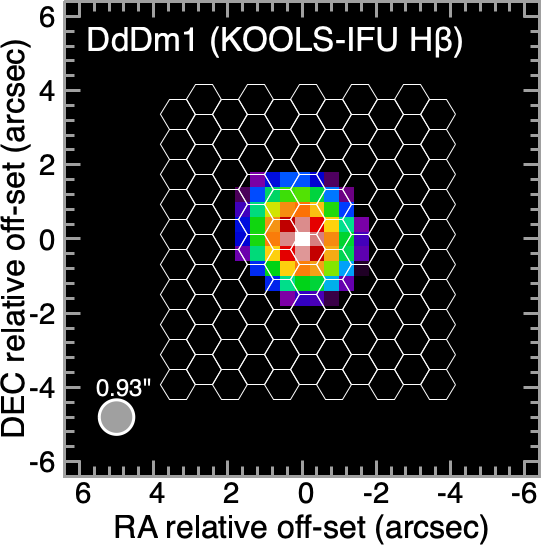
Figure 1: A dither position of the packed fiber array in KOOLS-IFU observations is overlaid on the PSF-deconvolved H$\beta$ emission image derived from the KOOLS-IFU data cube. The intensity scale is shown in logarithmic units, ranging from minimum to maximum. The gray circle represents the spatial resolution of the image. Each hexagon denotes the position and dimensions of the 110 fibers. Alt text: A PSF-deconvolved H$\beta$ emission image from the KOOLS-IFU dataset, overlaid with dithered positions of the packed fiber array.

2 Dataset and reduction

We explain the dataset and data reduction processes below. The logs of the spectroscopic observations are summarized in table 1.

2.1 Seimei/KOOLS-IFU observation

Table 1: Summary of spectroscopic observations for DdDm 1.

Date	Telescope/Inst.	Range ()	$R$
2024/07/21	Seimei/KOOLS-IFU	$0.400~-~0.853$	$\sim 820$
2024/07/21	Seimei/KOOLS-IFU	$0.560~-~1.010$	$\sim 900$
1990/09/06	IUE/SWP	$0.115~-~0.198$	$\sim 300$
1984/09/01,04	IUE/SWP	$0.115~-~0.198$	$\sim 300$
2008/07/08	Subaru/HDS	$0.39~-~0.66$	$\sim 72000$
2008/07/08	Subaru/HDS	$0.30~-~0.46$	$\sim 72000$
2006/05/11	Spitzer/IRS SL	$5.2~-~14.5$	$\sim 100$
2006/05/11	Spitzer/IRS SH, LH	$9.9~-~37.2$	$\sim 600$

We performed the dither-mapping observation (figure 1) using the Kyoto Okayama Optical Low-dispersion Spectrograph with optical-fiber integral field unit (KOOLS-IFU; Matsubayashi et al., 2019) attached to one of the two Nasmyth foci of the Kyoto University Seimei 3.8 m telescope (Kurita et al., 2020).

The observation was carried out under clear and stable sky conditions on 2024 July 21. The seeing, measured by the Shack–Hartmann camera, was $\sim 1{\arcsec}$ in the $R$-band at full width at half maximum (FWHM). The data were obtained at an airmass range of $1.01-1.09$ (average 1.04) for the VPH-blue setting and $1.19-1.51$ (average 1.35) for the VPH-red setting. We performed $7\times 300$ sec and $3\times 360$ sec exposures for the blue observations, and $6\times 300$ sec and $3\times 360$ sec exposures for the red observations, respectively. In each exposure, the data were taken with a sub-fiber pitch shift, increasing the spatial sampling from 0.8 spaxel^-1 to 0.4 spaxel^-1. Additionally, off-source frames were taken for background sky subtraction.

To perform flux calibration and remove telluric absorption, we observed HD192281 (O4.5V(n)) every 30 min using the same dithering pattern as employed for DdDm 1. To further evaluate light loss in the KOOLS-IFU field, BD+39 3026 (F5) nearby DdDm 1 was observed at every increase of 0.1 in airmass. We also obtained instrumental flat, twilight sky, and Hg/Ne/Xe-arc frames for baseline calibration.

2.2 Seimei/KOOLS-IFU data reduction

We reduced the data using our codes and IRAF (Tody, 1986) by following Otsuka (2022). Wavelength calibration was performed using over 40 Hg/Ne/Xe-arc lines that cover the full range of effective wavelengths. The resultant RMS errors in wavelength determination were 0.09 Å for the VPH-blue and 0.10 Å for the VPH-red. We adopted a constant plate scale of 2.5 Å. The average spectral resolution ($R$, defined as $\lambda$/Gaussian FWHM) measured from the arc lines was $\sim 820$ and $\sim 900$ for the VPH-blue and VPH-red spectra, respectively. We calibrated the extinction caused by airmass using the extinction magnitude-to-airmass ratio curve measured at Okayama Observatory in 2022. This curve was derived over the wavelength range of $4000-10000$ Å, with measurements taken at intervals of 2.5 Å.

We obtained an RA-DEC-wavelength datacube using our codes for image-data reconstruction based on the drizzle technique. We corrected the spatial displacements caused by atmospheric dispersion at each wavelength by following Otsuka (2022). We adopted a constant plate scale of 0.40 per spaxel, which provides a good signal-to-noise ratio (SNR) in each spaxel. During this procedure, we also generated the SNR map required for uncertainty evaluation for each wavelength image in the subsequent analyses. We evaluated the off-center value in RA and DEC relative to a reference position by measuring the center coordinates of the standard star in the 3-D datacube: the offset did not exceed 0.02 (0.05 pixel) in both directions over the wavelengths.

For flux calibration and telluric removal, we synthesized the non-LTE theoretical spectrum of HD192281 by fitting its archived Keck-II/ESI spectrum ($3850-9360$ Å, $R\sim 6200$ at 5020 Å; Sheinis et al., 2002) with the Tlusty code (Hubeny, 1988). We reduced the raw data (Program ID: W171, PI: Ferre-Mateu) downloaded from the Keck Observatory Archive webpage. By following a traditional fitting method with the aid of a genetic algorithm, we successfully determined seven elemental abundances, surface gravity ($\log_{10}\,g)=3.53$ cm s^-2, effective temperature ($T_{\rm eff})=38051$ K, and rotational velocity ($v\sin\,i$) = 298 km s^-1. We calculated the color excess between B and V bands, $E(B-V)=0.628$, toward HD192281 with a total-to-selective extinction $R_{\rm V}=3.1$ by comparing the synthesized spectrum and the Gaia BP/RP spectrum after spectral resolution matching. In this procedure, we adopted the reddening law of Cardelli et al. (1989). Flux calibration and telluric removal were simultaneously performed using the function derived by comparing this reddened telluric-free theoretical spectrum and the 1-D spectrum extracted from the observed 3-D datacube.

2.3 Seimei/KOOLS-IFU data point-spread function

We evaluated the achieved spatial resolution by measuring the Moffat function’s FWHM of the standard stars’ PSF at every wavelength. The Moffat function is represented as follows:

$$I(r) = \left[1+\left(r/{\alpha}\right)^{2}\right]^{-\beta},$$ (1)

$${\alpha} = {\rm FWHM}\left[2^{\left(1/{\beta}\right)}-1\right]^{-0.5},$$ (2)

where $I(r)$ is the radial profile of the PSF of the standard stars, and $\beta$ is the shape parameter and is fixed to 4.4 at all wavelengths. To correct for image quality degradation due to airmass, we adopted the equation established by Otsuka (2022). Consequently, the expected Moffat PSF’s FWHM of DdDm 1’s KOOLS-IFU images in arcsec can be expressed as a function of $\lambda$ in using equation (5).

$${\rm FWHM}=\left\{\begin{array}[]{ll}(1.67\pm 0.01)\,(\lambda/0.55)^{-0.18\pm 0.01}&\mbox{(blue)}\\ (1.90\pm 0.01)\,(\lambda/0.55)^{-0.17\pm 0.01}&\mbox{(red)}\end{array}\right.$$ (5)

After performing PSF matching in all spectral bins in the datacube using equation (5), we carried out spectral analysis.

2.4 Subaru/HDS spectrum of the central star

We investigate the natures of the central star with its high-dispersion echelle spectra taken using the High Dispersion Spectrograph (HDS; Noguchi et al., 2002) attached to one of Nasmyth foci of the Subaru 8.2 m telescope atop of Mt. Mauna Kea in Hawaii. We downloaded the archival raw data (PI: A. Tajitsu) from the Subaru Mitaka Okayama Kiso Archive (SMOKA). The observation was conducted under stable sky condition with a seeing of $\sim 0.6$ measured from the HDS slit-viewer camera. The slit-entrance has dimensions of 0.5 in width and 3.0 in length. Spectra were obtained using the blue and red cross dispersers, covering wavelength ranges of $2974-4610$ Å and $3945-5210$ Å, respectively. The image-de-rotators to keep position angle (P.A.) of 0 were used for both settings. For the red setting, we use an atmospheric dispersion corrector (ADC). We took a single 1800 sec exposure for both settings. We reduced the data with our codes and IRAF packages. We adopted a constant plate scale of 0.025 Å pixel^-1.

2.5 UV IUE and mid-infrared Spitzer spectra

We downloaded the SWP23840, 23872 (IUE program ID: GM115, PI: R.E.S. Clegg), and SWP39590 (ID: PNMMP, PI: M. Pẽna) obtained by the International Ultraviolet Explorer (IUE) from the Mikulski Archive for Space Telescopes (MAST). The IUE spectrum was used to derive the C²⁺ and N²⁺ ionic abundances from their collisionally excited lines (CELs). The size of the slit (9.9 $\times$ 22) covered the entire nebula of DdDm 1. We combined these spectra into a single $1150-1980$ Å spectrum using an SNR-weighted averaging method. The spectrum was then scaled to match the photometry measured from the Galaxy Evolution Explorer (GALEX; Bianchi et al., 2017) FUV channel image ($F_{\rm FUV}=(9.90\pm 0.10)\times 10^{-14}$ erg s^-1 cm^-2 Å^-1).

We also used the archived mid-IR Spitzer/Infrared Spectrograph (IRS; Houck et al., 2004) short-low (SL), short-high (SH), and long-high (LH) spectra (AOR key: 16808448 and 16808704, PI: K. B. Kwitter). The size of the slit was $3.7\arcsec\times 57\arcsec$ in SL, $4.7\arcsec\times 11.3\arcsec$ in SH, and $11.1\arcsec\times 22.3\arcsec$ in LH. These spectra were used to derive the Ne^+,2+, S^2+,3+, Ar^+,2+, and Fe²⁺ ionic abundances from their fine-structure lines and to examine dust features. We degraded the spectral resolution of the SH and LH spectra to match that of the SL spectrum and then combined these three spectra into a single spectrum. Finally, we scaled the flux density to match the mid-IR AKARI/IRC 18  band flux density ($F_{18\,{\micron}}=(2.16\pm 0.14)\times 10^{-12}$ erg s^-1 cm^-2 -1 ; Ishihara et al., 2010).

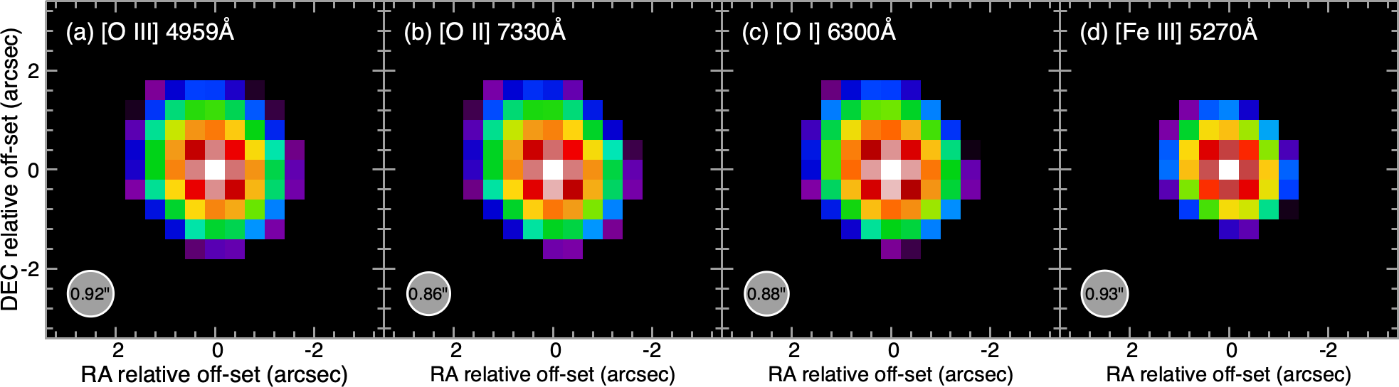
Figure 2: Selected PSF-deconvolved KOOLS-IFU emission-line images. The intensity is presented on a logarithmic scale, spanning from the minimum to the maximum values. The achieved spatial resolution is indicated by the gray circle. The spatial distribution of the [Fe iii] 5270 Å emission is much smaller in radius compared to that of the [O iii] 4959 Å emission, suggesting that a significant fraction of iron is locked in dust grains. See the main text for further details. Alt text: The PSF-deconvolved images of the four emission lines. The spatial distribution of the [Fe iii] line is more compact than that of [O iii], suggesting that a significant fraction of iron is locked in dust grains.

3 Results of the KOOLS-IFU observations

Before starting analyses, we check the accuracy of the data. We compare the flux density directly measured from the Pan-STARRS $r$-band image (downloaded from the Pan-STARRS1 data archive) with that derived from the synthesized $r$-band image created from the KOOLS-IFU datacube using the Pan-STARRS $r$-band filter transmission curve. The difference between the measured flux densities from both the two sources is only $\sim 0.7$ $\%$, with values of $(7.74\pm 0.02)\times 10^{-15}$ erg s^-1 cm^-2 Å^-1 for Pan-STARRS and $(7.69\pm 0.01)\times 10^{-15}$ erg s^-1 cm^-2 Å^-1 for KOOLS-IFU. Therefore, we can confidently conclude that our KOOLS-IFU data achieves sufficient accuracy in photometry.

3.1 Spatial distribution of emission lines

In figure 2, we present the images of the [O iii] 4959 Å, [O ii] 7330 Å, [O i] 6300 Å, and [Fe iii] 5270 Å lines, which are used to examine the ionization stratification and the spatial deficiency of ionized iron. These images were created by measuring the line fluxes in each spectrum for every spaxel using the automated line-fitting algorithm Alfa (Wesson, 2016), followed by a Lucy-Richardson PSF-deconvolution with fifteen iterations. To our knowledge, such emission-line images have never been presented before.

DdDm 1 is apparently very compact and exhibits a slightly elongated nebula with a position angle of $47{\degree}-52{\degree}$. This is consistent with the findings of Otsuka et al. (2009) and Henry et al. (2008), who demonstrated the elliptical nebular morphology of DdDm 1 using the broadband HST/WFPC1 F675W image. The three-sigma Gaussian radius along the major axis is estimated to be 1.03, 1.10, and 1.18 in [O iii], [O ii], and [O i], respectively. These values correspond to $3\times(\sigma_{\rm obs}^{2}-\sigma_{\rm res}^{2})^{0.5}$, where $\sigma_{\rm obs}$ denotes the Gaussian sigma of the emission-line distribution after PSF deconvolution, and $\sigma_{\rm res}$ represents the Gaussian sigma of the achieved spatial resolution. This calculation evaluates the intrinsic spatial extent of the emission-line distribution by accounting for and removing the broadening effects caused by seeing and instrumental resolution. Using these sub-arcsecond-resolution images, we confirm the ionization stratification, i.e., the nebular radius decreases as the ionization degree increases.

It is well known that the deficiency of elemental iron abundance relative to the Sun is consistently significantly lower than that of other elements, such as oxygen. This has been confirmed in ionized nebulae including PNe. Indeed, the present work derived [O/H] = $-0.64\pm 0.06$ and [Fe/H] = $-1.32\pm 0.13$ from our abundance analysis (subsection 6.3). This is because iron is a refractory element, while oxygen is a volatile element. Since iron atoms tend to exist as dust grains, we expect that the spatial distributions of ionized atomic iron emission lines in ionized nebulae are more compact than those of volatile elements, even with the same ionization degrees. We verify this through measurements of the spatial distributions of [O iii] 4959 Å (figure 2a) and the [Fe iii] 5270 Å (figure 2d). The spatial distribution of the [Fe iii] 5270 Å emission is noticeably more compact than that of the [O iii] 4959 Å emission; the three-$\sigma$ Gaussian radius along the major axis is 0.61 for [Fe iii] 5270 Å, which is approximately half of the 1.03 radius measured for [O iii] 4959 Å. At the [O iii] electron temperature $T_{\rm e}$([O iii]) and the [Cl iii] electron density $n_{\rm e}$([Cl iii]) (subsection 6.1), the volume emissivity of the [Fe iii] 5270 Å line is $(2.29\pm 0.81)\times 10^{-21}$ erg s^-1 cm³, while that of the [O iii] 4959 Å line is $(1.86\pm 0.03)\times 10^{-21}$ erg s^-1 cm³. Therefore, we infer that their spatial extent is not attributable to the difference in volume emissivity but rather to the difference in the spatial distributions of Fe²⁺ and O²⁺. This supports our expectation that iron emission lines are spatially more compact due to dust formation.

In many studies, the Fe abundance in ionized gas is determined using the Fe²⁺ abundance and the O/O²⁺ ratio. However, the spatial distribution differences between Fe²⁺ and O²⁺ must be considered; otherwise, the Fe abundance may inevitably be underestimated. Careful attention is required when interpreting the Fe abundance estimates.

3.2 Spatially-integrated 1D-spectrum

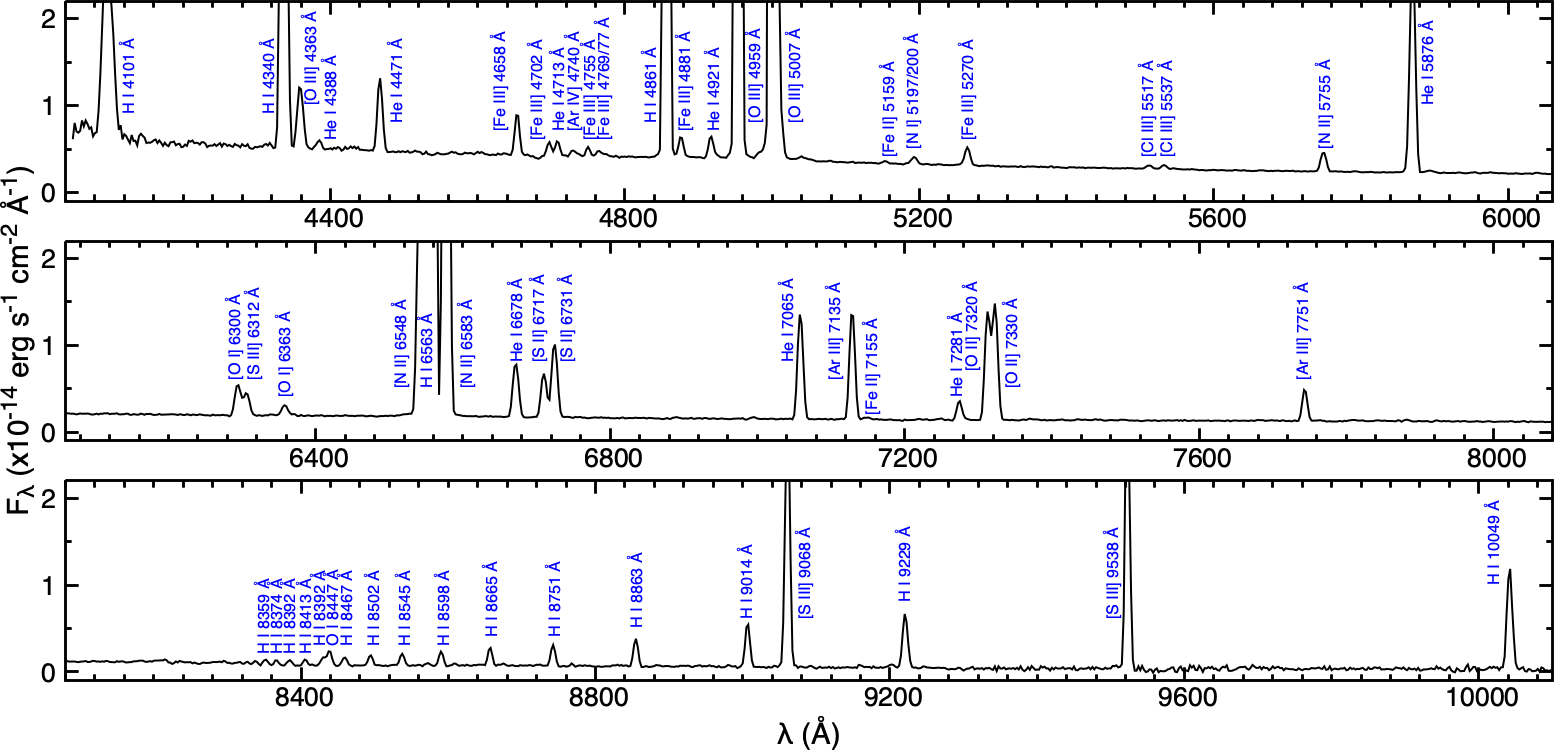
Figure 3: The KOOLS-IFU 1-D spectrum. Prominent lines among the identified emission lines are indicated in blue. The wavelengths are given in air and include a heliocentric correction. The dark-gray shaded region indicates the one-sigma uncertainty at each wavelength. Alt text: A spatially integrated 1-D spectrum generated from the KOOLS-IFU datacube. The horizontal and vertical axes are wavelength and flux density, respectively.

As shown in figure 3, we analyze the spatially integrated 1-D spectrum obtained from the KOOLS-IFU datacube. The spectrum is presented in air wavelengths with heliocentric corrections applied, and the heliocentric radial velocity is measured as $-308.2\pm 8.2$ km s^-1, consistent with Otsuka et al. (2009, $-309.14\pm 1.22$ km s^-1). Numerous prominent emission lines are clearly detected, while no carbon recombination lines are observed. This spectrum serves as the basis for the detailed analyses presented in the following sections.

4 Mid-infrared features

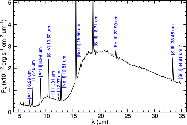
Figure 4: The Spitzer/IRS spectrum. The detected emission lines are indicated in blue. The wavelengths are given in vacuum. Alt text: The Spitzer/IRS spectrum. The horizontal and vertical axes are wavelength and flux density, respectively.

The Spitzer/IRS spectrum (figure 4) clearly shows two broad features attributed to amorphous silicate grains; the features centered at 9  and 18  are due to the Si-O stretching mode and the O-Si-O bending mode, respectively. Crystalline silicate emission are not detected in the spectrum around 11, 19.5, 23–24, 28, and 33.6 . Crystallization requires a re-heating process of amorphous dust. In the case of DdDm 1, this process is likely insufficient, resulting in the dominance of amorphous silicates. No carbon-based dust grains and molecules are not confirmed in the IRS spectrum. Therefore, DdDm 1 is certainly a O-rich dust PN.

5 Dust extinction and line flux measurement

We measure the line fluxes of atomic species in the 1-D KOOLS-IFU, IUE, and Spitzer spectra by fitting multiple Gaussian functions to their line profiles. The observed flux $F$($\lambda$) (and flux density $F_{\lambda}$) is reddened by both the interstellar and also the circumstellar dust. We obtain the dust extinction-free flux $I$($\lambda$) (and flux density $I_{\lambda}$) using equation (6):

$$I(\lambda) = F(\lambda)~\cdot~10^{c({\rm H\beta})(1+f(\lambda))},$$ (6)

where $c$(H$\beta$) ($=\log_{10}$ $I$(H$\beta$)/$F$(H$\beta$)) is the line-of-sight logarithmic reddening coefficient at H$\beta$ 4861.33 Å. The $c$(H$\beta$) value can be expressed as $1.45\,E(B-V)$ under $R_{\rm V}=3.1$ and the reddening law of Cardelli et al. (1989). The $E(B-V)$ value within a $2{\degree}\times 2{\degree}$ area centered on the coordinates of DdDm 1 is $(9.8\pm 0.7)\times 10^{-3}$, according to the Galaxy extinction map of Schlafly & Finkbeiner (2011). Thus, the $c$(H$\beta$) value is calculated to be $0.014\pm 0.001$. Note that this value originates from the average global interstellar dust over a large solid angle around DdDm 1, as the Galaxy extinction map is not high enough to resolve individual objects. Therefore, it is necessary to calculate the $c$(H$\beta$) value stemming from the combined contributions of interstellar and circumstellar dust. This can be achieved by comparing the observed extincted H i line fluxes with the corresponding extinction-free H i line fluxes, calculated using the H i emissivity of Storey & Hummer (1995) under the assumption of Case B. For this purpose, we employed H i lines detected in the KOOLS-IFU spectrum.

The H$\alpha$/H$\beta$ ratio is often assumed to be a constant value (e.g., 2.85), and this assumption is commonly used to calculate the $c$(H$\beta$) value. While this assumption is widely adopted as it simplifies calculations, it is not always appropriate. This is because the H i line emissivity depends on electron temperature ($T_{\rm e}$) and electron density ($n_{\rm e}$), which cannot be determined without performing plasma diagnostics based on de-reddened line fluxes. Correcting line reddening based on incorrect assumptions and using the resulting physical quantities for further discussion is problematic and potentially misleading. To avoid such issues and to derive a self-consistent $c$(H$\beta$) value, $T_{\rm e}$, and $n_{\rm e}$, it is essential to calculate them iteratively within a calculation loop. By iteratively refining these parameters, this approach ensures that the derived $c$(H$\beta$) value aligns consistently with the H i line emissivity determined by the plasma diagnostics, ultimately enabling more physically reliable interpretations.

This iterative loop for $c$(H$\beta$) derivation incorporates observed $T_{\rm e}$ and $n_{\rm e}$ diagnostic line fluxes, observed H i line fluxes, and the theoretical H i emissivity. For $T_{\rm e}$ diagnostics, we use the [O iii] lines at 4363, 4959, and 5007 Å. For $n_{\rm e}$ diagnostics, the [Cl iii] lines at 5517 Å and 5537 Å are selected, considering the ionization degree of [O iii] and [Cl iii]. We select the H i lines at 4101, 4340, 4863, 6563, 8665, 8751, 8863, 9229, and 10049 Å, using their eight ratios relative to H$\beta$. These H i lines are chosen to optimize dust reddening corrections across the KOOLS-IFU wavelength range. We keep $R_{\rm V}=3.1$ through our calculations.

The process begins by assuming an initial $c$(H$\beta$) value, set to 0 for the first iteration. Using this value, we apply reddening corrections to the [O iii] and [Cl iii] lines and determined $T_{\rm e}$([O iii]) and $n_{\rm e}$([Cl iii]). Theoretical H i line ratios are then calculated based on the derived $T_{\rm e}$([O iii]) and $n_{\rm e}$([Cl iii]). These theoretical ratios are compared with observed values, yielding eight individual $c$(H$\beta$) estimates. Outliers are removed via three-sigma clipping, and the mean of the remaining $c$(H$\beta$) values is computed. From the mean $c$(H$\beta$) and the remaining values along with their one-sigma uncertainties, the reduced-$\chi^{2}$ value is calculated. This process is iteratively repeated, updating the $c$(H$\beta$) value until the reduced-$\chi^{2}$ reaches its minimum (2.43).

Through this iterative approach, we derive $c$(H$\beta$) = $0.136\pm 0.013$, $T_{\rm e}$([O iii]) = $11896\pm 54$ K, and $n_{\rm e}$([Cl iii]) = $2536\pm 759$ cm^-3. The derived $c$(H$\beta$) value represents the combined contributions from both circumstellar and interstellar dust. Referring to Green et al. (2019), we estimate $c$(H$\beta$) value solely from the interstellar dust to be $0.04\pm 0.03$. By subtracting this interstellar component from the total $c$(H$\beta$) value of $0.136\pm 0.013$, we determine $c$(H$\beta$) = $0.098\pm 0.041$ as the contribution from circumstellar dust. For the extinction correction in following sections, we adopt the total value of $c$(H$\beta$) = $0.136\pm 0.013$.

In the 3-4th and 8-9th columns of table 6, we list the dereddened line fluxes normalized to the flux of H$\beta$, which is set to an intensity of 100: the observed quantities $I$(obs) and ${\delta}I$(obs) represent the normalized dereddened line fluxes and their one-$\sigma$ uncertainty, respectively. The dereddened H$\beta$ line flux $I$(H$\beta$) for the entire nebula is measured to be ($2.54\pm 0.08$)$\times 10^{-12}$ erg s^-1 cm^-2.

Table 2: Derived $T_{\rm e}$ and $n_{\rm e}$ in DdDm 1.

Parameter	$T_{\rm e}$ diagnostic line ratio	Value (K)
$T_{\rm e}$([O iii])	$I$(4959 Å+5007 Å)/$I$(4363 Å)	$11896~\pm~54$
$T_{\rm e}$([S iii])opt	$I$(9068 Å)/$I$(6312 Å)	$13179~\pm~626$
$T_{\rm e}$([S iii])opt/ir	$I$(9068 Å)/$I$(18.71 )	$13129~\pm~810$
$T_{\rm e}$([Ar iii])	$I$(7135 Å+7751 Å)/$I$(8.99 )	$11373~\pm~30$
$T_{\rm e}$([Fe iii])	$I$(4881)/$I$(22.90 )	$10911~\pm~1406$
$T_{\rm e}$([N ii])	$I$(6548 Å+6583 Å)/$I$(5755 Å)	$13192~\pm~247$
$T_{\rm e}$(He i)	He i lines	$11793~\pm~1241$
Parameter	$n_{\rm e}$ diagnostic line ratio	Value (cm-3)
$n_{\rm e}$([S iii])	$I$(18.71 )/$I$(33.48 )	$2656~\pm~722$
$n_{\rm e}$([Cl iii])	$I$(5517 Å)/$I$(5537 Å)	$2536~\pm~759$
$n_{\rm e}$([S ii])	$I$(6717 Å)/$I$(6731 Å)	$3454~\pm~879$

6 Plasma diagnostics

6.1 $T_{\rm e}$ and $n_{\rm e}$ derivations

Table 2 summarizes the derived $T_{\rm e}$ and $n_{\rm e}$ values. The $n_{\rm e}$ and $T_{\rm e}$ values from CELs are determined at the intersection points of the diagnostic $n_{\rm e}$–$T_{\rm e}$ curves for each ionization zone. The $T_{\rm e}$([O iii]), $T_{\rm e}$([Ar iii]), and $T_{\rm e}$([Fe iii]) values correspond to the intersection points of their respective $n_{\rm e}$–$T_{\rm e}$ curves with the one derived from $n_{\rm e}$([Cl iii]). Even when the $n_{\rm e}$–$T_{\rm e}$ curve derived from $n_{\rm e}$([S iii]) is used instead of $n_{\rm e}$([Cl iii]), these $T_{\rm e}$ values remain nearly identical. This consistency can be attributed to the fact that $n_{\rm e}$([S iii]) and $n_{\rm e}$([Cl iii]) diagnose similar physical conditions, resulting in comparable outputs.

Both $T_{\rm e}$([S iii])${\rm opt}$ and $T_{\rm e}$([S iii])${\rm opt/ir}$ correspond to the intersection points of their respective $n_{\rm e}$–$T_{\rm e}$ curves with the $n_{\rm e}$–$T_{\rm e}$ curve derived from $n_{\rm e}$([S iii]). Although they represent the same ionization stage, the calculated $T_{\rm e}$([S iii]) values are slightly higher than those of $T_{\rm e}$([O iii]), $T_{\rm e}$([Ar iii]), and $T_{\rm e}$([Fe iii]). This difference is likely caused by uncertainties in the flux calibration of [S iii] 9069 Å due to atmospheric extinction.

In the calculation of $T_{\rm e}$([N ii]), the recombination contribution of N²⁺ to the [N ii] 5755 Å line flux by following Liu et al. (2000) is first subtracted. The resulting $T_{\rm e}$([N ii]) value corresponds to the intersection point of its respective $n_{\rm e}$–$T_{\rm e}$ curve with the one derived from $n_{\rm e}$([S ii]).

$T_{\rm e}$(He i) has been calculated using the flux ratio of selected pairs of He i lines, such as He i at 7281, 6678, and 4921 Å (singlet lines) or 5876 Å and 4471 Å (triplet lines). However, as this method is highly optimized for the specific line pairs chosen, the ionic He⁺ abundances derived using $T_{\rm e}$(He i) and the He i line fluxes occasionally exhibit scatter among the different lines. As demonstrated by Otsuka et al. (2009), various He i ratios produce slightly differing $T_{\rm e}$(He i) values. To address the He⁺ abundance inconsistencies arising from $T_{\rm e}$(He i), we calculate a $T_{\rm e}$(He i) value that minimizes the scatter between the He⁺ abundances obtained from individual He i lines and the average He⁺ abundance derived across all He i lines. In this process, we utilize the $n_{\rm e}$–$T_{\rm e}$ logarithmic interpolation function of the He i effective recombination coefficients by Otsuka (2022) along with the $n_{\rm e}$ diagnostics and the $n_{\rm e}$ value determined from [Cl iii]. Notably, even if $n_{\rm e}$([S ii]) is used instead of $n_{\rm e}$([Cl iii]), the $T_{\rm e}$(He i) value remains essentially unchanged.

6.2 Ionic abundances

Table 3: Derived ionic abundances in DdDm 1.

Ion Xi+	Adopted $T_{\rm e}$/$n_{\rm e}$	$n$(Xi+)/$n$(H+)
He+ (5)	$T_{\rm e}$(He i)/$n_{\rm e}$([Cl iii])	$9.11\times 10^{-2}~\pm~6.61\times 10^{-3}$
C2+ (1)	$T_{\rm e}$([O iii])/$n_{\rm e}$([Cl iii])	$9.48\times 10^{-6}~\pm~1.40\times 10^{-6}$
N0 (1)	$T_{\rm e}$([N ii])/$n_{\rm e}$([S ii])	$2.46\times 10^{-7}~\pm~4.15\times 10^{-8}$
N+ (3)	$T_{\rm e}$([N ii])/$n_{\rm e}$([S ii])	$4.80\times 10^{-6}~\pm~1.88\times 10^{-7}$
N2+ (1)	$T_{\rm e}$([O iii])/$n_{\rm e}$([Cl iii])	$1.48\times 10^{-5}~\pm~2.74\times 10^{-6}$
O0+ (2)	$T_{\rm e}$([N ii])/$n_{\rm e}$([S ii])	$1.53\times 10^{-6}~\pm~8.32\times 10^{-8}$
O1+ (2)	$T_{\rm e}$([N ii])/$n_{\rm e}$([S ii])	$2.68\times 10^{-5}~\pm~5.84\times 10^{-6}$
O2+ (4)	$T_{\rm e}$([O iii])/$n_{\rm e}$([Cl iii])	$8.45\times 10^{-5}~\pm~1.18\times 10^{-6}$
Ne+ (1)	$T_{\rm e}$([N ii])/$n_{\rm e}$([S ii])	$8.14\times 10^{-6}~\pm~7.23\times 10^{-7}$
Ne2+ (1)	$T_{\rm e}$([O iii])/$n_{\rm e}$([Cl iii])	$1.67\times 10^{-5}~\pm~1.43\times 10^{-6}$
Si2+ (2)	$T_{\rm e}$([O iii])/$n_{\rm e}$([Cl iii])	$1.47\times 10^{-6}~\pm~2.07\times 10^{-7}$
S+ (2)	$T_{\rm e}$([N ii])/$n_{\rm e}$([S ii])	$1.61\times 10^{-7}~\pm~1.41\times 10^{-8}$
S2+ (4)	$T_{\rm e}$([S iii])opt/$n_{\rm e}$([S iii])	$1.13\times 10^{-6}~\pm~7.46\times 10^{-8}$
S3+ (1)	$T_{\rm e}$([S iii])opt/$n_{\rm e}$([S iii])	$2.41\times 10^{-7}~\pm~2.88\times 10^{-8}$
Cl2+ (2)	$T_{\rm e}$([O iii])/$n_{\rm e}$([Cl iii])	$1.64\times 10^{-8}~\pm~8.42\times 10^{-10}$
Ar1+ (1)	$T_{\rm e}$([N ii])/$n_{\rm e}$([S ii])	$6.56\times 10^{-8}~\pm~6.07\times 10^{-9}$
Ar2+ (3)	$T_{\rm e}$([Ar iii])/$n_{\rm e}$([Cl iii])	$4.38\times 10^{-7}~\pm~8.31\times 10^{-9}$
Ar3+ (1)	$T_{\rm e}$([Ar iii])/$n_{\rm e}$([Cl iii])	$2.92\times 10^{-8}~\pm~6.03\times 10^{-9}$
Fe2+ (5)	$T_{\rm e}$([Fe iii])/$n_{\rm e}$([Cl iii])	$6.37\times 10^{-7}~\pm~1.07\times 10^{-7}$

The ionic abundances $n$(Xⁱ⁺)/$n$(H⁺) are summarized in table 3. The number in parentheses in the 1st column indicates the number of emission lines used for each ionic abundance calculation. The ionic abundances except for the He⁺ abundance are determined by solving the population equations for multiple energy levels using the $T_{\rm e}$ and $n_{\rm e}$ values listed in the second column. When multiple lines are available, the ionic abundance is calculated for each line individually, followed by a three-sigma clipped averaging of the results. By following Liu et al. (2000), the respective O⁺ and N⁺ abundances derived from the [O ii] 7320/7330 Å and [N ii] 5755 Å lines are corrected for the recombination contribution from O²⁺ and N²⁺. In calculating Xⁱ⁺/H⁺, the $T_{\rm e}$ and $n_{\rm e}$ values for H⁺ are assumed to be the same as those for the co-existing Xⁱ⁺.

6.3 Elemental abundances

Table 4: Comparisons between elemental abundances in DdDm 1 and the AGB nucleosynthesis result.

X	$n$(X)/$n$(H)	$12+\log_{10}\,$$n$(X)/$n$(H)					[X/H]
	this work	this work	Ref.(1)	Ref.(2)	Ref.(3)	AGB model	this work
He	$9.11\times 10^{-2}~\pm~6.61\times 10^{-3}$	$10.96~\pm~0.03$	$10.95$	$10.97~\pm~0.06$	$11.01~\pm~0.04$	$10.98$	$+0.03~\pm~0.03$
C	$1.27\times 10^{-5}~\pm~2.10\times 10^{-6}$	$7.10~\pm~0.07$	$7.05$	$7.05~\pm~0.20$	$7.02~\pm~0.06$	$7.66$	$-1.33~\pm~0.09$
N	$1.99\times 10^{-5}~\pm~2.74\times 10^{-6}$	$7.30~\pm~0.06$	$7.40$	$7.40~\pm~0.11$	$7.36~\pm~0.02$	$7.47$	$-0.53~\pm~0.08$
O	$1.13\times 10^{-4}~\pm~5.96\times 10^{-6}$	$8.05~\pm~0.02$	$8.06$	$8.06~\pm~0.09$	$8.07~\pm~0.01$	$8.01$	$-0.64~\pm~0.06$
Ne	$2.52\times 10^{-5}~\pm~2.49\times 10^{-6}$	$7.40~\pm~0.04$	$7.24$	$7.32~\pm~0.08$	$7.45~\pm~0.01$	$7.27$	$-0.53~\pm~0.11$
Si	$1.96\times 10^{-6}~\pm~3.13\times 10^{-7}$	$6.29~\pm~0.07$	$\cdots$	$6.25~\pm~0.13$	$6.58~\pm~0.15$	$6.85$	$-1.22~\pm~0.08$
S	$1.53\times 10^{-6}~\pm~2.53\times 10^{-7}$	$6.19~\pm~0.07$	$6.35$	$6.31~\pm~0.12$	$6.35~\pm~0.01$	$6.46$	$-0.94~\pm~0.08$
Cl	$2.00\times 10^{-8}~\pm~1.94\times 10^{-9}$	$4.30~\pm~0.04$	$4.69$	$4.42~\pm~0.10$	$4.61~\pm~0.08$	$4.53$	$-1.20~\pm~0.30$
Ar	$5.33\times 10^{-7}~\pm~3.10\times 10^{-8}$	$5.73~\pm~0.03$	$5.16$	$5.81~\pm~0.10$	$5.79~\pm~0.09$	$5.74$	$-0.67~\pm~0.13$
Fe	$1.52\times 10^{-6}~\pm~4.65\times 10^{-7}$	$6.18~\pm~0.13$	$\cdots$	$\cdots$	$6.58~\pm~0.14$	$6.84$	$-1.32~\pm~0.13$

Note – The C abundance are derived from CELs. Solar abundances are taken from Asplund et al. (2009). The AGB model result is taken from Karakas et al. (2018) where adopts the following values for the initial elemental abundances: He:10.92, C:7.75, N:7.15, O:8.01, Ne:7.25, Si:6.83, S:6.44, Cl:4.51, Ar:5.72, Fe:6.82.
References – (1) Wesson et al. (2005); (2) Henry et al. (2008); (3) Otsuka et al. (2009).

Table 4 summarizes the derived elemental abundance $n$(X)/$n$(H) and $12+\log_{10}\,$$n$(X)/$n$(H). We emphasize that the values presented here are based on spectro-photometry of the entire nebula with absolutely no flux loss.

The elemental abundances are calculated by introducing the ionization correction factor (ICF) for each element X. ICFs account for the ionic abundances of unobserved ionization stages within the observed spectral coverage. $n$(X)/$n$(H) can be expressed as ICF(X)$\cdot$$\sum n$(Xⁱ⁺)/$n$(H⁺)_obs, where $n$(Xⁱ⁺)/$n$(H⁺)_obs refers to the ionic abundances derived from the observed spectra. The ICF values for He, N, O, S, and Ar are set to unity because the central star of DdDm 1 has a low temperature, meaning the nebular He²⁺, N³⁺, O³⁺, S⁴⁺, and Ar⁴⁺ abundances are expected to be negligible. For both C and Si, the ICF is given as $n$(O)/$n$(O²⁺). For Ne, it is $n$(O)/($n$(O⁺) + $n$(O²⁺)). The ICF for Cl is $n$(Ar)/$n$(Ar²⁺). For Fe, we adopt the ICF presented by Delgado Inglada et al. (2009). The last column of table 4 shows the enhancement of each element with respect to solar abundances, where we refer to Asplund et al. (2009).

7 Gas-to-Dust mass ratio, gas and dust masses

We estimate the gas-to-dust mass ratio (GDR, $\psi$) and the gas/dust masses ($m_{\rm g}$/$m_{\rm d}$) following Otsuka (2022). When gas and dust grains coexist in the same volume, $\psi$ can be expressed as follows:

$$\psi = \frac{C(\log_{10}\,e)\kappa_{{\rm H}\beta}}{c({\rm H}\beta)_{\rm cir}}\cdot\sum\frac{4\pi I_{g}\mu_{g}}{n_{\rm e}j_{\rm g}(T_{\rm e},n_{\rm e})},$$

$$\kappa_{{\rm H}\beta} = \frac{\int_{min}^{max}\pi a^{2}Q_{\rm ext}({\rm H}\beta,a)n(a)da}{\int_{min}^{max}\frac{4}{3}\pi a^{3}\rho_{\rm d}n(a)da},$$ (7)

where $C$ is a dimensionless constant: assuming that the nebular shape is circular with a radius $r=1$ (subsection 3.1) when projected on sky, and it equals $\pi^{-1}(4.848\times 10^{-6}~r)^{-2}$. $\kappa_{{\rm H}\beta}$ is the mass extinction coefficient. $Q_{\rm ext}$(H$\beta$,$a$) is the extinction coefficient of a grain with radius $a$ at H$\beta$. $\rho_{\rm d}$ is the mass density of the grain (2.228 g cm^-3). We adopt the optical constant of amorphous silicate grain taken from Laor & Draine (1993). $n(a)$ is the grain size distribution; we adopt $n(a)\propto a^{-3.5}$. We calculate the $\kappa_{{\rm H}\beta}$ value of $3.99\times 10^{4}$ cm² g^-1 between the maximum radius 0.25  and the minimum radius 0.03  by following Mie theory. $c$(H$\beta$)_cir is the extinction coefficient at H$\beta$ stemming from circumstellar dust (i.e., $0.098\pm 0.041$ estimated in section 5). $n{\rm g}$ and $\mu_{\rm g}$ denote the number density and atomic weight of the target gas, respectively. $j_{\rm g}$($T_{\rm e}$,$n_{\rm e}$) represents the volume emissivity of the gas component per $n_{\rm g}n_{\rm e}$. $I_{\rm g}$ is the observed extinction-free line flux of the gas component. In calculating GDR, we utilize the H i and He i lines. For each ion, we adopt the same $T_{\rm e}$ and $n_{\rm e}$ values listed in table 2. Then, we obtain GDR of $619\pm 102$.

Next, using equation (8), we directly calculate the total atomic gas mass $m_{\rm g}$ of $(1.26\pm 0.15)\times 10^{-3}$ $D_{\rm kpc}^{2}$ $f$ M_⊙, where $D_{\rm kpc}$ is the distance in kpc and $f$ is a correction factor for the gas density assuming a uniform distribution (i.e., filling factor of the gas and dust emitting volume).

$$m_{\rm g} = \sum\frac{4\pi D^{2}I_{g}\mu_{g}f}{n_{\rm e}j_{\rm g}(T_{\rm e},n_{\rm e})}.$$ (8)

Using the derived $m_{\rm g}$ and GDR values, we estimate the dust mass $m_{\rm d}$ to be $(4.05\pm 0.86)\times 10^{-6}$ $D_{\rm kpc}^{2}$ $f$ M_⊙. We use equation (8) to avoid uncertainties related to the unknown geometric structure of the emitting region, under the assumption that the gas is uniformly distributed.

So far, the only report on GDR in DdDm 1 comes from the pioneering work of Hoare & Clegg (1988). This study employed silicate dust radiative transfer models adopting $n(a)\propto a^{-3.5}$ with $a$ ranging from 0.005 to 0.25 , and obtained a GDR of 769 by fitting to the IRAS four-band flux densities. However, the IRAS 12  and 100  flux densities are upper limits, while the uncertainties for the 25  and 60  flux densities would be 30 $\%$ or greater. Since silicate dust peaks at 9  and 18 , the uncertainties in the 12  and 25  data would undoubtedly have a significant impact on the model fitting. Thus, the GDR reported by Hoare & Clegg (1988) likely includes an uncertainty of at least $\sim 30$ $\%$, leading to their GDR = $769\pm 230$. If we adopt $a=0.005-0.25$  with $n(a)\propto a^{-3.5}$, we derive the GDR of $481\pm 79$. In both $a$ ranges, our derived GDR values are consistent with that of Hoare & Clegg (1988) within one-$\sigma$ uncertainty.

8 Discussion

8.1 Comparison of elemental abundances

We compare our results for DdDm 1 with three previously conducted observations in the 4-6th columns of table 4. The used datasets are as follows: Henry et al. (2008) utilized spectro-photometry obtained by a long-slit with a slit-width of 5 putting along P.A. = 90, Otsuka et al. (2009) employed an echelle spectrum obtained with a slit-width of 0.6 and an ADC, and Wesson et al. (2005) used a long-slit spectrum obtained by a long-slit with a slit-width of 0.9 putting along P.A. = 0, without an ADC. While our result is in excellent agreement with Henry et al. (2008), significant discrepancies of approximately a factor of two in the Cl abundance are seen when compared to the others. We examine the causes of these discrepancies.

First, we consider the discrepancy between our results and those of Otsuka et al. (2009). This discrepancy likely arises from differences in the spectral extraction region and the adopted $c$(H$\beta$) value. The KOOLS-IFU spatially integrated 1-D spectra encompass the entire nebula, whereas Otsuka et al. (2009) focused on the bright central region. The [Cl iii] line maps generated from KOOLS-IFU reveal that their spatial distributions are concentrated in the central region and are more compact than that of the H$\beta$ line. Therefore, we speculate that the flux ratio of [Cl iii] to H$\beta$ lines in Otsuka et al. (2009) is larger than our results. To verify this hypothesis, we extracted a pseudo-spectrum from the KOOLS-IFU datacube, simulating the slit dimensions used by Otsuka et al. (2009), and measured the flux ratio $F$([Cl iii] 5537 Å)/$F$(H$\beta$). Our measurement reproduces their results well: $0.302\pm 0.060$ in the pseudo-spectrum compared to $0.357\pm 0.050$ reported by Otsuka et al. (2009). Thus, we conclude that the differences in observational methods and spatial extraction regions are the primary reasons for the discrepancy in the chlorine abundance measurements.

Next, we address the discrepancy with Wesson et al. (2005). While this discrepancy may partly arise from differences in the spectral extraction regions, a significant issue lies in the detection of the [Cl iii] 5537 Å line itself. They report detecting only the [Cl iii] 5537 Å line; however, this is highly unusual. This is because the [Cl iii] 5517 Å line flux is comparable to that of [Cl iii] 5537 Å line in DdDm 1, as confirmed by all other observational results. In our observation, the ratio of [Cl iii] $F$(5517 Å) to $F$(5537 Å) is $0.969\pm 0.060$, which is consistent with previous measurements. The [Cl iii] $F$(5517 Å)/$F$(5537 Å) ratio indicates that both lines should be detectable with comparable fluxes. Therefore, the reported detection of only the [Cl iii] 5537 Å line in Wesson et al. (2005) strongly suggests inaccuracies in their measurement, and the Cl abundance derived from their results cannot be considered reliable.

Wesson et al. (2005) did not calculate the Ne⁺ abundance and adopted a higher $T_{\rm e}$ value than ours for the Ar²⁺ abundance derivation. As a result, noticeable discrepancies in Ne and Ar abundances are found between Wesson et al. (2005) and ours. The discrepancies in Si and Fe abundances between Otsuka et al. (2009) and our results are due to differences in the adopted ICFs: Otsuka et al. (2009) used the O/O⁺ ratio, whereas we adopt the O/O²⁺ ratio for Si and 1.1 (O⁺/O²⁺)^0.58 (O/O⁺) from Delgado Inglada et al. (2009) for Fe. Thus, we account for the abundance discrepancies observed between previous studies and our results.

In summary, our results align with previous observations and can be regarded as representative elemental abundance values for DdDm 1. Furthermore, we recognize that spatial coverage is critical for accurately estimating abundances in PNe.

8.2 Comparison with AGB nucleosynthesis models

The most notable characteristics of DdDm 1 are its extremely low carbon abundance and low metallicity. The [Ar/H] value (see the last column of table 4) indicates that the metallicity of DdDm 1 is comparable to that of the Small Magellanic Cloud (SMC). Argon, a noble gas not synthesized in nucleosynthesis processes within progenitor stars, is resistant to depletion onto dust grains or molecules, making it a robust tracer of metallicity. To the best of our knowledge, DdDm 1 is the most carbon-deficient PN in the Milky Way. Carbon is synthesized during the AGB phase and transported to the stellar surface through the TDUs, a mixing process triggered by He-shell instabilities or thermal pulses.

According to the theoretical AGB nucleosynthesis models by Karakas et al. (2018) (see table 4), the efficiency of the TDUs increases significantly in stars with initial masses of $\sim 1.15$ M_⊙ or higher, particularly at the SMC metallicity. TDU events enrich the stellar surface with carbon and other elements, with this enrichment becoming more pronounced in stars with initial masses up to $\sim 3-4$ M_⊙. The extraordinarily low carbon abundance of DdDm 1 strongly indicates that its progenitor star had an initial mass of less than 1.15 M_⊙. In fact, the model by Karakas et al. (2018) predicts no TDU in such stars. Instead, it shows that during the thermal pulse AGB phase, the isotope ratios of C, N, and O undergo slight changes due to the effects of weak convection, the CNO cycle, or very weak and inefficient TDUs. These changes can explain the observed C and N abundances in DdDm 1: C is slightly depleted, while N is slightly enhanced relative to their initial values. Similarly, the absence of significant surface enrichment of Ne as well as C and O further supports the conclusion that DdDm 1 did not experience efficient TDU events. Nitrogen is typically enhanced through the CNO cycle during earlier phases, such as the red giant branch (RGB) phase, and/or through the hot bottom burning (HBB) process during the late AGB phase. However, the HBB process only occurs in stars with initial masses of $\sim 3$ M_⊙ or higher, ruling out its contribution to DdDm 1. While uncertainties in the derived carbon abundance—such as potential observational errors or model assumptions—should be considered, the observed elemental abundances in DdDm 1 are consistent with the predictions of the AGB model for a star with an initial mass of 1.0 M_⊙ by Karakas et al. (2018). To the best of our knowledge, this is the first evidence showing that both the model and observations conclusively rule out TDUs in DdDm 1.

The lower [Si,Fe/H] values compared to the [Ar/H] values suggest that both elements are likely sequestered in dust grains, consistent with their depletion in the gas phase.

In conclusion, DdDm 1 most likely evolved from a progenitor star with an initial mass of $\sim 1.0$ M_⊙. The observed carbon abundance suggests that the progenitor star formed in an extremely carbon-poor environment and evolved as a single star, without undergoing mass accretion events such as binary mass transfer or coalescence during its evolution. DdDm 1 did not experience efficient TDUs. Furthermore, the nebular abundances appear to closely reflect the initial composition of the progenitor star, making DdDm 1 a particularly interesting intriguing PN. It provides observational evidence that PNe can form and evolve even from stars with such low initial masses.

8.3 Post-AGB evolution of the central star

We infer the post-AGB evolution of the central star. Henry et al. (2008) suggest that the central star is a He-shell burner. However, the Subaru HDS spectrum of the central star (figure 5) clearly exhibits the stellar absorption lines attributed to H i, He i, and He ii. Thus, we assume that the H-shell burning can sustain the luminosity of the central star after the AGB phase.

We synthesize a post-AGB evolution track for a star with an initial mass of 1.0 M_⊙ and $Z=0.0028$, corresponding to SMC metallicity. As presented in figure 6 (c) and (d), we create the evolution track by interpolating between the theoretical post-AGB evolution tracks for 1.0 M_⊙ stars with $Z$ = 0.010 and 0.001 provided by Miller Bertolami (2016). Previous studies have reported $T_{\rm eff}$ values ranging from 37000 to 55000 K (see table 1 of Otsuka et al., 2009); Based on this, two possible evolutionary statuses can be considered: (1) the central star is still evolving toward the whitedwarf (WD) cooling track, with its temperature increasing; or (2) the central star has already entered the WD cooling track, with its temperature decreasing.

The nebular spectrum of DdDm 1 shows neither He ii nebular emission lines nor mid-infrared molecular hydrogen (H₂) emission. Additionally, we confirm that the central star spectrum obtained with Subaru HDS displays narrow absorption lines, indicating low surface gravity. Consistently, McCarthy et al. (1997) directly measured $\log_{10}\,g$ = 3.4 cm s^-2 using a Keck HIRES spectrum of DdDm 1. These characteristics are inconsistent with those typically observed in PNe whose central stars have already entered the WD cooling track. Most of PNe in the WD cooling track show He ii nebular emission lines, their central star spectra exhibit broad absorption lines.

If the central star is in the WD cooling track with $T_{\rm eff}\leq 46000$ K, $L_{\ast}$ and $\log_{10}\,g$ would be $\leq 1.25$ L_⊙ and $\geq 7.7$ cm s^-2, respectively, according to our synthesized evolution track for a star with initially 1.0 M_⊙ and $Z=0.0028$. Using the distance estimate derived from our luminosity budget method (subsection 8.5), the distance to DdDm 1 would then be $\leq 0.42$ kpc. At this distance, the outer radius of the nebula would correspond to only $\leq 0.002$ pc, which is unacceptably small and physically implausible. Furthermore, $\log_{10}\,g\geq 7.7$ cm s^-2 cannot explain the absorption profile of the observed spectrum of the central star at all.

The central star of DdDm 1 did not evolve as a hydrogen burner but may have undergone a born-again event during the post-AGB phase, similar to Hen 3-1357 (the Stingray Nebula; see Otsuka et al., 2017, for details). Hen 3-1357 is an O-rich PN that exhibits 9/18  silicate emission in its Spitzer/IRS spectrum and is shows short-term variations in $\log_{10}\,g$, $T_{\rm eff}$, and $L_{\ast}$ (Parthasarathy et al., 1993; Reindl et al., 2014, 2017; Balick et al., 2021; Peña et al., 2022). However, no evidence of such variations, such as changes in surface gravity, effective temperature, or luminosity, has been observed in DdDm 1, making this scenario unlikely.

In summary, the central star of DdDm 1 as a H-burner is currently evolving toward the WD cooling track, with its temperature increasing while maintaining nearly constant luminosity.

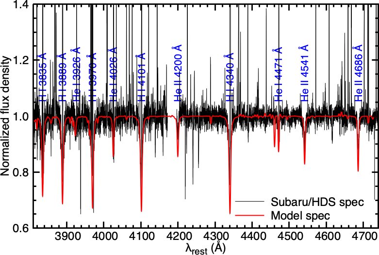
Figure 5: Comparison between the Subaru/HDS spectrum of the central star and its non-LTE theoretical spectrum synthesized with the Tlusty code (Hubeny, 1988). In the fitting procedure, the nebular elemental abundances (see table 4), $T_{\rm eff}$ of 41639 K, and $\log_{10}\,g$ of 3.93 cm s^-2 derived from our photoionization model (see table 5 in subsection 8.6) are adopted. Alt text: Comparison between the Subaru/HDS spectrum of the central star and its theoretically calculated spectrum. The horizontal and vertical axes are wavelength and normalized flux density, respectively.

8.4 Ejected total gas mass

In the synthesized evolutionary tracks, $L_{\ast}$ and $\log_{10}\,g$ are established as a function of $T_{\rm eff}$ for each. For a $T_{\rm eff}$ range of $37000-55000$ K, the corresponding ranges for $L_{\ast}$ and $\log_{10}\,g$ are $4725-4877$ L_⊙ and $3.72-4.43$ cm s^-2, respectively. Karakas et al. (2018) predict that a star with an initial mass of 1.0 M_⊙ and $Z=0.0028$ will evolve into a central star with a final mass of 0.651 M_⊙ after ejecting 0.349 M_⊙. Similarly, Miller Bertolami (2016) predict that stars with an initial mass of 1.0 M_⊙ and $Z=0.001$ and $Z=0.010$ will evolve into central stars with core masses of $\sim 0.55$ M_⊙ and $\sim 0.53$ M_⊙, respectively, implying mass ejection of $\sim 0.45-0.47$ M_⊙.

In summary, stars including the progenitor of DdDm 1 with an initial mass of 1.0 M_⊙ and $Z=0.0028$ are expected to eject $\sim 0.35-0.47$ M_⊙ during their evolution. These predicted values - $T_{\rm eff}$, $L_{\ast}$, $\log_{10}\,g$, and the ejected mass - will serve as constraints for the photoionization modeling (subsection 8.6).

8.5 Emitting volume of gas and dust emission

The nebular luminosity from ionized and atomic gas and dust grains should be in principle equal to the luminosity of the central star. If the nebular luminosity is less than that of the central star, it suggests that the ionization boundary is determined by the material distribution, the filling factor is less than unity, or possibly both. Otsuka et al. (2009) assumed that the nebula is material-bounded to reproduce the observed line fluxes in their photoionization model adopting $D=10$ kpc and $T_{\rm eff}=39000$ K, $L_{\ast}=2000-3000$ L_⊙, $\log_{10}\,g=5.0$ cm s^-2, and $f=1.0$. In the case of DdDm 1, we think that the nebular boundary is determined not by the material distribution but by the radiation field of the central star because the KOOLS-IFU spectrum exhibits neutral atomic emission lines such as [O i].

Here, we assume that filling factor can be expressed as the ratio of the nebular luminosity to the central star luminosity. This means $f$ can be expressed as a function of $D_{\rm kpc}$ and $L_{\ast}$. We obtain the nebular luminosity using (1) a theoretically synthesized nebular continuum (2.22 $D_{\rm kpc}^{2}$ L_⊙, integrated in $0.1-10^{4}$ ), (2) a modified two-temperature blackbody fitting (60.3 K and 117.6 K) with the grain-size weight-average $Q_{\rm ext}$($\lambda$,$a$) (for $a=0.03-0.25$  and an $a^{-3.5}$ size distribution) applied to the Spitzer IRS spectrum (1.61 $D_{\rm kpc}^{2}$ L_⊙), and (3) theoretical calculations of emission line fluxes (3.59 $D_{\rm kpc}^{2}$ L_⊙), where we consider H i ($2-1$, $n-2$, and $n-3$ transitions, where $n$ is the principal quantum number, up to $n=40$), He i, $[$C iii$]$ + C iii$]$, [N i, ii, iii], [O i, ii, iii], [Ne ii, iii], [Si iii], [S ii, iii, iv], [Cl iii], and [Ar ii, iii, iv].

Thus, in the range of $T_{\rm eff}=37000-55000$ K, we find $f$ is $\sim 0.35-0.60$ in $L_{\ast}$ = $4725-4877$ L_⊙ and $D=15-22$ kpc. Especially, adopting $D=20$ kpc (subsection 3.1) and $L_{\ast}=4800$ L_⊙ leads to $f=0.62$, and we obtain $m_{\rm g}=(0.31\pm 0.04)$ M_⊙ and using equation (8) and $m_{\rm d}=(1.00\pm 0.21)\times 10^{-3}$ M_⊙ using equation (7). This $m_{\rm g}$ value satisfies with the theoretically predicted total ejected mass $\sim 0.35-0.47$ M_⊙ (subsection 8.4).

8.6 Photoionization modeling

Table 5: The adopted and derived parameters in the Cloudy model.

Central star	Value
$T_{\rm eff}$	41639 K
$L_{\ast}$	4848 L⊙
$\log_{10}\,g$	3.93 cm s-2
$D$	19.39 kpc
Nebula	Value
elemental abundances	He: 10.98, C: 6.92, N: 7.37, O: 8.06,
(12 + $\log_{10}$$n$(X)/$n$(H))	Ne: 7.53, Si: 6.23, S: 6.26, Cl: 4.24,
	Ar: 5.71, Fe: 6.37,
	others: Karakas et al. (2018)
geometry	spherical shell nebula
	inner radius = 47.3 au
	ionization boundary radius = 19742 au
	(=1.0 arcsec)
$n(r)$	4486 cm-3
filling factor	0.510
$I$(H$\beta$)	$2.55\times 10^{-12}$ erg cm-2 s-1
total gas mass	0.287 M⊙
Silicate dust grain	Value
temperature	$50-1230$ K
total dust mass	$3.78\times 10^{-4}$ M⊙
GDR	760
Reduced-$\chi^{2}$	22.01

We construct a photoionization model to reproduce all observed quantities (line fluxes, flux densities, and nebular radius) and the derived physical parameters, ensuring consistency with the post-AGB evolutionary model for stars with initially 1 M_⊙ and $Z=0.0028$, within the measurement uncertainties. We use the photoionization code Cloudy (v17.03; Ferland et al., 2017).

8.6.1 Modeling approach

As discussed in subsection 8.3, the central star is currently evolving toward a white dwarf with increasing effective temperature. Referring to previous works, $T_{\rm eff}$ is estimated to range from 37000 K to 55000 K, and $\log_{10}\,g$ is $\sim 4.0$ cm s^-2. Hence, as the incident SED, we adopt theoretical spectra of non-LTE line-blanketed model atmospheres of O-type stars by Lanz & Hubeny (2003). This grid model is suitable for DdDm 1 in the ranges of $T_{\rm eff}$ and $\log_{10}\,g$ ranges. We set the photospheric elemental abundances to [X/H] = $-0.70$, except for He (He/H=0.10). We have established two distinct functions: one for $L_{\ast}$ and another for $\log_{10}\,g$, both are as functions of $T_{\rm eff}$. Given a $T_{\rm eff}$ value, $L_{\ast}$ and $\log_{10}\,g$ are uniquely determined along the predicted post-AGB evolutionary track for 1 M_⊙ stars with $Z=0.0028$. We treat the distance $D$ as a free parameter, allowing it to vary within the range of $15-22$ kpc.

We adopt a spherically symmetric nebula with a constant hydrogen radial profile $n(r)$ as a function of $r$, the distance from the central star and the ionization boundary is determined by the radiation from the central star. Given $L_{\ast}$ and $D$ values, the filling factor $f$ is uniquely determined using the observed nebular luminosity, as explained in subsection 8.5.

We begin the modeling with the empirically determined elemental abundances (see table 4) as input values. These abundances are then varied within their three-$\sigma$ uncertainties to achieve the best-fit model. Throughout the iterative process, the abundances of undetected elements lighter than zinc are fixed to the values predicted by Karakas et al. (2018) for 1.0 M_⊙ stars with $Z=0.0028$.

We adopt spherical amorphous silicate grain with $a=0.03-0.25$  following $a^{-3.5}$ size distribution. We adopt the optical constant of Laor & Draine (1993). The radius range is divided into 30 bins. For each bin, Cloudy calculates the absorption efficiency $Q_{\rm abs}$ and scattering efficiency $Q_{\rm sca}$ based on Mie theory. The resulting $Q_{\rm abs}$ and $Q_{\rm sca}$ values are then used in the model calculations.

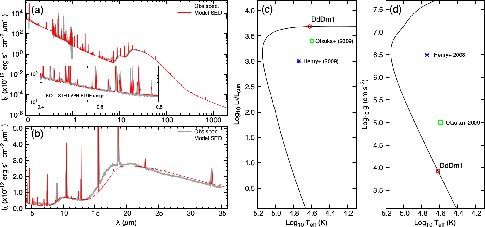
Figure 6: (left two panels) Comparison between the observed spectra and the predicted SED by the best model. Panel (a) displays the $0.1-2000$  range SED. The inset focuses on the $0.4-0.8$  range. Panel (b) focuses on the $5-40$  range. (right two panels) The current location of the central star predicted by Cloudy modeling is plotted on the $\log_{10}\,T_{\rm eff}-\log_{10}\,L_{\ast}$/L_⊙ plane (panel c) and the $\log_{10}\,T_{\rm eff}-\log_{10}\,g$ plane (panel d). The theoretical post-AGB evolutionary track for 1.0 M_⊙ stars with $Z=0.0028$ (black line, synthesized using the data from Miller Bertolami (2016)) is plotted on both planes. The values reported by Henry et al. (2008, Henry+ 2008) and Otsuka et al. (2009, Otsuka+ 2009) are also included. Alt text: The left two panels display a comparison of the observed spectra with the theoretically calculated spectrum. The right two panels display the location of the central star on the theoretically predicted $\log_{10}\,T_{\rm eff}-\log_{10}\,L_{\ast}$/L_⊙ and $\log{10}\,T_{\rm eff}-\log_{10}\,g$ planes. Both the theoretical post-AGB evolutionary track and the values from the two prior studies are plotted on these planes.

We vary the following 14 free parameters until the model achieves the best: $T_{\rm eff}$, $D$, the inner radius of the nebula, GDR, and 10 elemental abundances (He/C/N/O/Ne/Si/S/Cl/Ar/Fe). Iterative calculations are terminated either when the nebular gas temperature drops below 4000 K or when the predicted total gas mass to 0.47 M_⊙ (subsection 8.4). The quality of the fit is assessed based on the reduced-$\chi^{2}$ value, calculated from 97 observational constraints: the H$\beta$ flux $I$(H$\beta$) (observed value: ($2.54\pm 0.08$)$\times 10^{-12}$ erg s^-1 cm^-2, see section 5), 69 gas emission line fluxes relative to $I$(H$\beta$), 25 mid-infrared Spitzer/IRS flux densities, GDR (observed value: $619\pm 102$, see subsection 7), and the ionization boundary radius of 1.0 (subsection 3.1). In the reduced-$\chi^{2}$ calculation, we exclude the He i 7065 Å line because its reduced-$\chi^{2}$ value is large (708): the enhancement of collisional excitation for this line is important. Except for the [O i] and [N i] lines, we adopt the one-$\sigma$ uncertainty. For the [O i] and NI lines, we set their uncertainty to 30 $\%$. Referring to the Spitzer/IRS handbook, we adopt a one-$\sigma$ uncertainty of 6 $\%$ for Band IRS01-09, which are covered by the SL module, and 10 $\%$ for the other bands, which are covered by the SH and LH modules (see table 6). For the ionization boundary radius (i.e., the outer radius of the nebula), we adopt the one-$\sigma$ uncertainty of 30 $\%$.

8.6.2 Model results

Table 6: Comparison between the observed and the CLOUDY model predicted values.

Species	$\lambda$	$I$(obs)	${\delta}I$(obs)	$I$(Cloudy)	Species	$\lambda$	$I$(obs)	${\delta}I$(obs)	$I$(Cloudy)
		$I$(H$\beta$)=100.000					$I$(H$\beta$)=100.000
O iii$]$	1666.15 Å	$7.070$	$1.082$	$6.625$	[S ii]	6716.44 Å	$2.733$	$0.101$	$2.733$
[N iii]	1744-54 Å	$4.432$	$0.798$	$6.604$	[S ii]	6730.82 Å	$4.630$	$0.106$	$4.829$
[Si iii]	1882.71 Å	$4.455$	$0.993$	$6.354$	He i	7065.22 Å	$6.403$	$0.109$	$9.300$
[Si iii]	1892.03 Å	$5.504$	$0.892$	$5.122$	[Ar iii]	7135.79 Å	$6.463$	$0.123$	$8.205$
$[$C iii$]$+C iii$]$	1906/09 Å	$13.374$	$1.912$	$13.434$	He i	7281.35 Å	$1.105$	$0.059$	$1.015$
H i	4101.73 Å	$24.296$	$1.385$	$26.344$	[O ii]	7318/19 Å	$6.234$	$0.249$	$8.865$
H i	4340.46 Å	$44.855$	$0.807$	$47.498$	[O ii]	7330/31 Å	$6.576$	$0.250$	$7.113$
[O iii]	4363.00 Å	$4.758$	$0.366$	$5.546$	[Ar iii]	7751.11 Å	$1.690$	$0.066$	$1.968$
He i	4471.49 Å	$5.188$	$0.275$	$5.026$	H i	8358.96 Å	$0.258$	$0.055$	$0.178$
[Fe iii]	4658.01 Å	$2.390$	$0.105$	$2.413$	H i	8374.43 Å	$0.236$	$0.047$	$0.202$
[Fe iii]	4701.62 Å	$0.775$	$0.062$	$0.902$	H i	8392.35 Å	$0.282$	$0.032$	$0.231$
[Ar iv]+He i	4711/13 Å	$0.882$	$0.039$	$1.037$	H i	8413.28 Å	$0.290$	$0.064$	$0.266$
[Fe iii]	4733.84 Å	$0.331$	$0.029$	$0.314$	H i	8437.91 Å	$0.467$	$0.064$	$0.310$
[Ar iv]	4740.12 Å	$0.146$	$0.029$	$0.189$	H i	8467.21 Å	$0.421$	$0.022$	$0.365$
[Fe iii]	4754.64 Å	$0.513$	$0.023$	$0.441$	H i	8502.44 Å	$0.482$	$0.026$	$0.435$
[Fe iii]	4769.52 Å	$0.328$	$0.024$	$0.302$	H i	8545.34 Å	$0.547$	$0.026$	$0.526$
[Fe iii]	4777.61 Å	$0.162$	$0.023$	$0.149$	H i	8598.35 Å	$0.698$	$0.044$	$0.645$
H i	4861.33 Å	$100.000$	$1.000$	$100.000$	H i	8664.98 Å	$0.803$	$0.053$	$0.805$
[Fe iii]	4881.12 Å	$1.225$	$0.061$	$1.035$	H i	8750.43 Å	$0.985$	$0.041$	$1.023$
He i	4921.93 Å	$1.204$	$0.060$	$1.306$	H i	8862.74 Å	$1.304$	$0.064$	$1.330$
[O iii]	4958.91 Å	$146.137$	$2.046$	$145.454$	H i	9014.87 Å	$1.999$	$0.116$	$1.775$
[O iii]	5006.84 Å	$433.515$	$6.069$	$433.973$	[S iii]	9068.62 Å	$12.643$	$0.455$	$15.019$
[Fe ii]	5158.78 Å	$0.182$	$0.037$	$0.261$	H i	9228.97 Å	$2.557$	$0.138$	$2.448$
[N i]	5199/5201 Å	$0.492$	$0.148$	$0.174$	H i	10049.3 Å	$5.626$	$0.225$	$5.315$
[Fe iii]	5270.40 Å	$1.197$	$0.087$	$1.848$	[Ar ii]	6.98	$0.928$	$0.082$	$0.259$
[Cl iii]	5517.71 Å	$0.200$	$0.011$	$0.163$	H i	7.46	$3.316$	$0.295$	$1.959$
[Cl iii]	5537.87 Å	$0.206$	$0.008$	$0.226$	[Ar iii]	8.99	$4.730$	$0.402$	$5.113$
[N ii]	5755.00 Å	$1.269$	$0.037$	$1.248$	[S iv]	10.51	$9.170$	$0.779$	$5.260$
He i	5875.64 Å	$13.486$	$0.216$	$14.852$	H i	11.31	$0.225$	$0.036$	$0.237$
[O i]	6300.30 Å	$1.982$	$0.595$	$1.881$	H i	12.37	$0.716$	$0.068$	$0.719$
[S iii]	6312.06 Å	$1.476$	$0.063$	$1.600$	[Ne ii]	12.81	$7.173$	$0.610$	$9.642$
[O i]	6363.78 Å	$0.695$	$0.209$	$0.601$	[Ne iii]	15.55	$27.673$	$2.325$	$29.057$
[N ii]	6548.05 Å	$15.071$	$2.788$	$15.853$	[S iii]	18.71	$13.778$	$1.171$	$14.627$
H i	6562.81 Å	$266.334$	$8.789$	$277.210$	[Fe iii]	22.92	$1.855$	$0.326$	$1.905$
[N ii]	6583.45 Å	$46.602$	$1.351$	$46.732$	[S iii]	33.47	$6.196$	$0.527$	$4.285$
He i	6678.15 Å	$3.517$	$0.070$	$3.681$
Band	$\lambda$	$F_{\nu}$(obs)	${\delta}F_{\nu}$(obs)	$F_{\nu}$(Cloudy)	Band	$\lambda$	$F_{\nu}$(obs)	${\delta}F_{\nu}$(obs)	$F_{\nu}$(Cloudy)
		(mJy)					(mJy)
IRS01	5.00	$2.992$	$0.180$	$2.201$	IRS14	19.00	$334.000$	$33.400$	$309.500$
IRS02	6.00	$3.871$	$0.232$	$2.321$	IRS15	20.00	$364.600$	$36.460$	$351.700$
IRS03	7.00	$4.673$	$0.280$	$2.560$	IRS16	21.00	$396.100$	$39.610$	$387.200$
IRS04	8.00	$5.148$	$0.309$	$4.108$	IRS17	22.00	$426.400$	$42.640$	$421.800$
IRS05	9.00	$11.940$	$0.716$	$12.380$	IRS18	23.00	$446.600$	$44.660$	$449.700$
IRS06	10.00	$20.080$	$2.008$	$22.070$	IRS19	24.00	$458.500$	$45.850$	$478.200$
IRS07	11.00	$25.610$	$2.561$	$25.870$	IRS20	25.00	$468.300$	$46.830$	$502.600$
IRS08	12.00	$26.110$	$2.611$	$29.200$	IRS21	26.00	$480.800$	$48.080$	$522.200$
IRS09	13.00	$26.000$	$2.600$	$32.200$	IRS22	27.00	$499.300$	$49.930$	$538.500$
IRS10	15.00	$84.760$	$8.476$	$61.960$	IRS23	28.00	$519.400$	$51.940$	$551.400$
IRS11	16.00	$150.100$	$15.010$	$105.100$	IRS24	29.00	$530.900$	$53.090$	$562.400$
IRS12	17.00	$224.900$	$22.490$	$168.400$	IRS25	30.00	$533.500$	$53.350$	$568.900$
IRS13	18.00	$291.100$	$29.110$	$241.900$

Table 5 summarizes all the input parameters and the derived quantities in the best model. The dust grain temperature peaks at $a=0.03$  in the innermost layer of the nebula (1230 K) and reaches its minimum at $a=0.25$  in the outermost layer (50 K). Table 6 provides a detailed comparison between the observed and model-derived line fluxes and dust continuum flux density. The reduced-$\chi^{2}$ value of 22.01 is comparable to that achieved in the model of H4-1 based on KOOLS-IFU data (Otsuka et al., 2023). Thus, we conclude that our model reproduces these observed quantities within acceptable accuracy. Figure 6a presents a comparison of the SED between the observed spectra and the best model across a wide wavelength range. The inset demonstrates that the model provides a remarkably good fit to the $0.4-0.8$  range observed with KOOLS-IFU.

Figure 6b focuses on the Spitzer/IRS wavelength range for a detailed comparison. The model reproduces the observed SED well, except for the $\sim 13-20$  range, where an offset is identified. The dust formed in O-rich environment is expected to consist of silicates, magnesium/iron oxide grain (e.g., Mg_1-xFe_xO, $x=0-1$; Henning et al., 1995), and aluminum oxide (Al₂O₃). Al₂O₃, with its higher condensation temperature, forms in the inner, high-temperature region of the O-rich circumstellar envelope, while silicates condense in regions further out (e.g., Gail & Sedlmayr, 1999; Ferrarotti & Gail, 2006). Mg_1-xFe_xO forms in the intermediate region between the formation zones of Al₂O₃ and silicates. Notably, Mg_1-xFe_xO and amorphous Al₂O₃ are known to exhibit emission in the $\sim 17-18$  range. However, its peak position does not coincide with the offset’s central wavelength of $\sim 16$ . This offset is therefore considered to result from the weighting applied to fitting procedure. Aside from the $\sim 13-20$  range, the SED fitting performs well, and the overall fitting is regarded as successful.

Figures 6c and d show the derived $T_{\rm eff}$, $\log_{10}$ ($L_{\ast}$/L_⊙), and $\log_{10}\,g$ plotted on the theoretical $T_{\rm eff}-\log_{10}$ ($L_{\ast}$/L_⊙) and $T_{\rm eff}-\log_{10}\,g$ diagrams, respectively. The derived values lie perfectly on the theoretical post-AGB evolutionary track for 1.0 M_⊙ stars with $Z=0.0028$. Both Henry et al. (2008) and Otsuka et al. (2009) conclude that DdDm 1 evolved from a $\sim$1 M_⊙ star. Their predicted $T_{\rm eff}/L_{\ast}/\log_{10}\,g$ values are 55000 K/1000 L_⊙/6.5 cm s^-2 in Henry et al. (2008), and 39000 K/$2000-3000$ L_⊙/5.0 cm s^-2 in Otsuka et al. (2009). It is obvious that neither Henry et al. (2008) nor Otsuka et al. (2009) aligns with the predicted post-AGB track for such stars.

The derived $m_{g}$ of 0.287 M_⊙ represents the mass within the ionization boundary radius, which includes a small fraction of neutral atomic gas. In subsection 8.4, the progenitor star is expected to have ejected a total mass of $\sim 0.35-0.47$ M_⊙. Our model explains $\sim 61-82$ $\%$ of the mass-loss history, with $\sim 0.06-0.18$ M_⊙ of neutral gas likely lying beyond the ionization front.

How much dust did the progenitor star produce during its evolution? If the model-predicted GDR of 760 is applicable to the entire nebula including the neutral gas region, and the AGB model predicted total gas mass is $\sim 0.35-0.47$ M_⊙, the progenitor star would have produced $(4.61-6.18)\times 10^{-4}$ M_⊙ of dust. By comparison, Ferrarotti & Gail (2006) constructed a theoretical dust production model for stars with an initial mass of 1.0 M_⊙ and $Z=0.004$. Their model predicts that such stars eject a total mass of 0.335 M_⊙, including a dust mass of $2.53\times 10^{-4}$ M_⊙, composed of $1.75\times 10^{-4}$ M_⊙ silicate and $7.80\times 10^{-5}$ M_⊙ iron dust. Our derived total dust mass is consistent with Ferrarotti & Gail (2006), considering the uncertainties in both our CLOUDY model and the theoretical model of Ferrarotti & Gail (2006).

In short, we successfully constructed a highly sophisticated model for DdDm 1, surpassing previous models in completeness. Our model reproduces all observed quantities related to the gas, dust, and central star within a single framework. Furthermore, the estimated origin and evolution of the progenitor star of DdDm 1, as well as the masses of gas and dust ejected during its evolution, are consistent with the latest theoretical models, making this achievement particularly noteworthy.

9 Summary

We investigated the origin and evolution of the Galactic halo PN DdDm 1 using the newly obtained Seimei/KOOLS-IFU spectra combined with multiwavelength spectra. Through our detailed analyses, we constructed a comprehensive model that elucidates the physical and chemical processes of this PN.

The KOOLS-IFU emission line images achieve $\sim 0.9$ arcsec resolution, resolving the elliptical nebula and revealing a compact spatial distribution of the [Fe iii] line compared to the [O iii] line, despite their similar volume emissivities. This indicates that iron, with its higher condensation temperature than oxygen, is easily incorporated into dust grains such as silicate, making the iron abundance estimate prone to underestimation. Using a fully data-driven approach, we directly derive ten elemental abundances, the gas-to-dust mass ratio, and the gas and dust masses based on our own distance scale and the emitting volumes of gas and dust. DdDm 1 evolved from a star of initial mass of $\sim$1.0 M_⊙ in a low-metallicity environment ($Z=0.18$ Z_⊙) characterized by a significant carbon deficiency. The observed elemental abundances are well consistent with predictions from AGB nucleosynthesis models. DdDm 1 is particularly rare due to its low C/O ratio and very low C abundance. While other halo PNe with low C/O ratios, such as PRMT 1 (e.g, Pena et al., 1990) and NGC 4361 (e.g., Torres-Peimbert et al., 1990), have been reported, DdDm 1 stands out as one of the most extreme cases, as it evolved into a PN without experiencing efficient TDU during its evolution. Our photoionization model reproduces all observed quantities in excellent agreement with predictions from AGB nucleosynthesis, post-AGB evolution, and AGB dust production models.

Our study offers new insights into the evolution and PN formation pathway of low-mass, metal-deficient stars like DdDm 1 and underscores the role of PN progenitors in the chemical enrichment of the Galaxy.

I am grateful to the referee for a careful reading and valuable suggestions.

I dedicate this paper to my beloved father, Nobujiro Otsuka. Throughout his life, my father stood as my unwavering pillar of strength, believing in me and encouraging me under all circumstances. He was not only the person I respected the most, but also the foundation of all my achievements and the guiding light that shaped who I am today. His steadfast love, wisdom, and support enabled me to accomplish all my research.

I also dedicate this paper to my PhD supervisor, Professor Shin’ichi Tamura. He was like a parent in my academic journey. DdDm 1 is one of the planetary nebulae he first introduced to me at the start of my graduate studies, and it has held a special place in my heart. DdDm 1 is a cherished object that holds the memories of his guidance, wisdom, and the time we shared together.

I was supported by the Japan Society for the Promotion of Science (JSPS) Grants-in-Aids for Scientific Research (C) (19K03914 and 22K03675).

References

- Asplund et al. (2009) Asplund, M., Grevesse, N., Sauval, A. J., & Scott, P. 2009, ARA&A, 47, 481
- Balick et al. (2021) Balick, B., Guerrero, M. A., & Ramos-Larios, G. 2021, ApJ, 907, 104
- Bianchi et al. (2017) Bianchi, L., Shiao, B., & Thilker, D. 2017, ApJS, 230, 24
- Cardelli et al. (1989) Cardelli, J. A., Clayton, G. C., & Mathis, J. S. 1989, ApJ, 345, 245
- Clegg et al. (1987) Clegg, R. E. S., Peimbert, M., & Torres-Peimbert, S. 1987, MNRAS, 224, 761
- Delgado Inglada et al. (2009) Delgado Inglada, G., Rodríguez, M., Mampaso, A., & Viironen, K. 2009, ApJ, 694, 1335
- Ferland et al. (2017) Ferland, G. J., Chatzikos, M., Guzmán, F., et al. 2017, Rev. Mexicana Astron. Astrofis., 53, 385
- Ferrarotti & Gail (2006) Ferrarotti, A. S., & Gail, H. P. 2006, A&A, 447, 553
- Gail & Sedlmayr (1999) Gail, H. P., & Sedlmayr, E. 1999, A&A, 347, 594
- Green et al. (2019) Green, G. M., Schlafly, E., Zucker, C., Speagle, J. S., & Finkbeiner, D. 2019, ApJ, 887, 93
- Henning et al. (1995) Henning, T., Begemann, B., Mutschke, H., & Dorschner, J. 1995, A&AS, 112, 143
- Henry et al. (2008) Henry, R. B. C., Kwitter, K. B., Dufour, R. J., & Skinner, J. N. 2008, ApJ, 680, 1162
- Hoare & Clegg (1988) Hoare, M. G., & Clegg, R. E. S. 1988, MNRAS, 235, 1049
- Houck et al. (2004) Houck, J. R., Roellig, T. L., van Cleve, J., et al. 2004, ApJS, 154, 18
- Hubeny (1988) Hubeny, I. 1988, Computer Physics Communications, 52, 103
- Ishihara et al. (2010) Ishihara, D., Onaka, T., Kataza, H., et al. 2010, A&A, 514, A1
- Jacoby et al. (2017) Jacoby, G. H., De Marco, O., Davies, J., et al. 2017, ApJ, 836, 93
- Karakas et al. (2018) Karakas, A. I., Lugaro, M., Carlos, M., et al. 2018, MNRAS, 477, 421
- Kurita et al. (2020) Kurita, M., Kino, M., Iwamuro, F., et al. 2020, PASJ, 72, 48
- Kwok (2000) Kwok, S. 2000, The Origin and Evolution of Planetary Nebulae (Cambridge University Press)
- Lanz & Hubeny (2003) Lanz, T., & Hubeny, I. 2003, ApJS, 146, 417
- Laor & Draine (1993) Laor, A., & Draine, B. T. 1993, ApJ, 402, 441
- Liu et al. (2000) Liu, X. W., Storey, P. J., Barlow, M. J., et al. 2000, MNRAS, 312, 585
- Matsubayashi et al. (2019) Matsubayashi, K., Ohta, K., Iwamuro, F., et al. 2019, PASJ, 71, 102
- McCarthy et al. (1997) McCarthy, J. K., Mendez, R. H., & Kudritzki, R. P. 1997, in IAU Symposium, Vol. 180, Planetary Nebulae, ed. H. J. Habing & H. J. G. L. M. Lamers, 120
- Miller Bertolami (2016) Miller Bertolami, M. M. 2016, A&A, 588, A25
- Noguchi et al. (2002) Noguchi, K., Aoki, W., Kawanomoto, S., et al. 2002, PASJ, 54, 855
- Otsuka (2022) Otsuka, M. 2022, MNRAS, 511, 4774
- Otsuka et al. (2009) Otsuka, M., Hyung, S., Lee, S.-J., Izumiura, H., & Tajitsu, A. 2009, ApJ, 705, 509
- Otsuka et al. (2015) Otsuka, M., Hyung, S., & Tajitsu, A. 2015, ApJS, 217, 22
- Otsuka et al. (2008) Otsuka, M., Izumiura, H., Tajitsu, A., & Hyung, S. 2008, ApJ, 682, L105
- Otsuka et al. (2017) Otsuka, M., Parthasarathy, M., Tajitsu, A., & Hubrig, S. 2017, ApJ, 838, 71
- Otsuka et al. (2010) Otsuka, M., Tajitsu, A., Hyung, S., & Izumiura, H. 2010, ApJ, 723, 658
- Otsuka et al. (2023) Otsuka, M., Ueta, T., & Tajitsu, A. 2023, PASJ, 75, 1280
- Parker et al. (2016) Parker, Q. A., Bojičić, I. S., & Frew, D. J. 2016, in Journal of Physics Conference Series, Vol. 728, Journal of Physics Conference Series, 032008
- Parthasarathy et al. (1993) Parthasarathy, M., Garcia-Lario, P., Pottasch, S. R., et al. 1993, A&A, 267, L19
- Peña et al. (2022) Peña, M., Parthasarathy, M., Ruiz-Escobedo, F., & Manick, R. 2022, MNRAS, 515, 1459
- Peña et al. (1993) Peña, M., Torres-Peimbert, S., Peimbert, M., & Dufour, R. J. 1993, Rev. Mexicana Astron. Astrofis., 27, 175
- Pena et al. (1990) Pena, M., Ruiz, M. T., Torres-Peimbert, S., & Maza, J. 1990, A&A, 237, 454
- Pena et al. (1991) Pena, M., Torres-Peimbert, S., & Ruiz, M. T. 1991, PASP, 103, 865
- Pena et al. (1992) —. 1992, A&A, 265, 757
- Rauch et al. (2002) Rauch, T., Heber, U., & Werner, K. 2002, A&A, 381, 1007
- Reindl et al. (2017) Reindl, N., Rauch, T., Miller Bertolami, M. M., Todt, H., & Werner, K. 2017, MNRAS, 464, L51
- Reindl et al. (2014) Reindl, N., Rauch, T., Parthasarathy, M., et al. 2014, A&A, 565, A40
- Schlafly & Finkbeiner (2011) Schlafly, E. F., & Finkbeiner, D. P. 2011, ApJ, 737, 103
- Sheinis et al. (2002) Sheinis, A. I., Bolte, M., Epps, H. W., et al. 2002, PASP, 114, 851
- Storey & Hummer (1995) Storey, P. J., & Hummer, D. G. 1995, MNRAS, 272, 41
- Tody (1986) Tody, D. 1986, in Society of Photo-Optical Instrumentation Engineers (SPIE) Conference Series, Vol. 627, Instrumentation in astronomy VI, ed. D. L. Crawford, 733
- Torres-Peimbert & Peimbert (1979) Torres-Peimbert, S., & Peimbert, M. 1979, Rev. Mexicana Astron. Astrofis., 4, 341
- Torres-Peimbert et al. (1990) Torres-Peimbert, S., Peimbert, M., & Pena, M. 1990, A&A, 233, 540
- Wesson (2016) Wesson, R. 2016, MNRAS, 456, 3774
- Wesson et al. (2005) Wesson, R., Liu, X. W., & Barlow, M. J. 2005, MNRAS, 362, 424
- Zijlstra et al. (2006) Zijlstra, A. A., Gesicki, K., Walsh, J. R., et al. 2006, MNRAS, 369, 875