How to choose efficiently the size of the Bethe-Salpeter Equation Hamiltonian for accurate exciton calculations on supercells

Abstract

The Bethe-Salpeter Equation (BSE) is the workhorse method to study excitons in materials. The size of the BSE Hamiltonian, that is how many valence to conduction band transitions are considered in those calculations, needs to be chosen to be sufficiently large to converge excitons’ energies and wavefunctions but should be minimized to make calculations tractable, as BSE calculations scale with the number of atoms as $(N_{\rm{atoms}}^{6})$. In particular, in the case of supercell (SC) calculations composed of $N_{\rm{rep}}$ replicas of the primitive cell (PC), a natural choice to build this BSE Hamiltonian is to include all transitions from PC calculations by zone folding. However, this greatly increases the size of the BSE Hamiltonian, as the number of matrix elements in it is $(N_{k}N_{c}N_{v})^{2}$, where $N_{k}$ is the number of $k$-points, and $N_{c(v)}$ is the number of conduction (valence) states. The number of $k$-points decreases by a factor $N_{\rm{rep}}$ but both the number of conduction and valence states increase by the same factor, therefore the BSE Hamiltonian increases by a factor $N_{\rm{rep}}^{2}$, making exactly corresponding calculations prohibitive. Here we provide an analysis to decide how many transitions are necessary to achieve comparable results. With our method, we show that to converge with an energy tolerance of 0.1 eV the first exciton binding energy of a LiF SC composed of 64 PCs, we only need 12% of the valence to conduction transitions that are given by zone folding. We also show that exciton energies are much harder to converge than Random Phase Approximation transition energies, underscoring the necessity of careful convergence studies. The procedure in our work helps in evaluating excitonic properties in large SC calculations such as defects, self-trapped excitons, polarons, and interfaces.

I Introduction

Ab initio calculations of crystals are widely used in the materials science community. Most of those techniques use crystal periodicity and Bloch’s theorem to understand the electronic properties of materials. However, there are several cases of interest where the translational symmetry is broken, such as defects [1], amorphous materials [2, 3, 4], self-trapped excitons [5, 6], frozen phonon calculations [7], polarons [8], and surfaces [2, 9]. In this kind of situation, it is common to use a supercell (SC) approximation [10] where the SC size must be large enough to converge the desired properties [11, 12], such as electronic energy levels and phonon frequencies. The SC consists of $N_{\rm{rep}}$ replicas of one PC. The SC size is limited in practice by the available computational resources, therefore schemes to overcome this difficulty are necessary. In particular, if the atoms are only slightly moved from their original positions due to a symmetry breaking, such as local strains and defects, then SC properties are still similar to PC properties, which can be used to construct an approximation.

DFT studies using the SC approximation are already common [10], but GW and Bethe-Salpeter Equation (BSE) calculations are less common due to their high computational cost [1, 13, 14, 15, 16]. The GW method [17] is known to have better performance in reproducing the experimental bandgaps of semiconductors, while BSE [18] is successful in studying excitonic effects. GW/BSE calculations are performed on top of DFT results and are, in general, more computationally demanding than DFT calculations and their convergence is harder to achieve. Typical plane-wave DFT calculations scale with $\mathcal{O}(N_{\rm{atoms}}^{3})$ [19], while GW/BSE calculations scale up to $\mathcal{O}(N_{\rm{atoms}}^{6})$ [20], where $N_{\rm{atoms}}$ is the total number of atoms. Despite the recent advances in parallelism efficiency [1], new theories and approaches are still necessary in order to avoid computationally demanding calculations. The stochastic pseudobands method facilitates the convergence of GW calculations [21]. The dielectric function can also be evaluated using analytical models, avoiding several numerical calculations [22, 23]. Scissor-operators are also a valid option in the case where the GW corrections follow approximately a linear relation with DFT energy levels [24, 20]. Subsampling schemes deal with $\mathbf{G}$-vectors perpendicular to the layers of 2D systems greatly reducing the density of $\mathbf{k}$-point sampling the first BZ [25] for both GW and BSE calculations. One can also expand wavefunctions of SC on the basis of wavefunctions of PC, and then calculate SC kernel matrix elements in terms of PC kernel matrix elements [26, 27, 28]. Dai et. al have developed a perturbation method that combines finite-momentum excitons and phonons to study polaronic excitons without the necessity of SCs [29, 30]. Tight-binding versions of BSE also provide a significant speed-up but need to be parametrized very accurately [31, 32, 33, 34].

In this work we focus on the BSE calculations, and more specifically on the kernel matrix elements calculations, which contain the electron-hole interaction and is the most computationally demanding step of our SC GW/BSE calculations. The main convergence issue in this kind of calculation is to choose how many conduction and valence bands are included in the BSE Hamiltonian. The number of bands can increase greatly, increasing the number of necessary node-hours and RAM memory to perform those calculations, as well as the amount of memory to store wavefunctions and GW/BSE results, making BSE calculations on SCs computationally very challenging. We provide a proper way of choosing the number of valence and conduction for SC based on results of PC results. Within our scheme we built a BSE Hamiltonian, which size is 12% of the size of a BSE Hamiltonian built based only the zone folding of PC states. With this scheme we achieved kernel calculations 8.4 times faster with errors of 0.1 eV for the binding energies of SC compared to PC results.

We chose to study LiF because … LiF is an insulator with strong excitonic effects that are well studied theoretically [18]. Due to the strong electron-phonon interaction, polaronic effects are strong as well [35, 36], and it presents self-trapped excitons with polaronic character [29, 30] and color centers [37, 38, 39].

The paper is organized in the following way: in section II we discuss the zone-folding aspects to be considered in BSE calculations and our approach, in section III we provide computational details of our calculations, in section IV we show our approach applied to LiF SC calculations, and in section VI we present our conclusions.

II Theory

In this section, we discuss what should be considered when going from PC to SC calculations. The $k$-point sampling and the total number of $\bf{G}$-vectors concepts are common for both DFT and GW/BSE calculations, therefore we start discussing them in the case of DFT. Let’s consider a crystal with lattice vectors $\boldsymbol{a_{1}},\boldsymbol{a_{2}}$ and $\boldsymbol{a_{3}}$ and reciprocal lattice vectors $\boldsymbol{b_{1}},\boldsymbol{b_{2}}$ and $\boldsymbol{b_{3}}$ that obey $\boldsymbol{a_{i}}\cdot\boldsymbol{b_{j}}=2\pi\delta_{ij}$. If a SC has lattice vectors $N_{1}\boldsymbol{a_{1}}$, $N_{2}\boldsymbol{a_{2}}$, and $N_{3}\boldsymbol{a_{3}}$, with $N_{i}\geq 1$ being a natural number, then the primitive reciprocal lattice vectors are given by $\boldsymbol{b_{1}}/N_{1}$, $\boldsymbol{b_{2}}/N_{2}$, $\boldsymbol{b_{3}}/N_{3}$. Therefore, the SC volume increases by a factor $N_{\rm{rep}}=N_{1}N_{2}N_{3}$, while the first Brillouin Zone (BZ) reciprocal volume decreases by this same factor. To make the results of a SC calculation comparable to results from primitive cell (PC) calculations, one needs to make sure that the density of $k$-points grids in both BZs is consistent, or in other words, the number $N_{k}^{SC}$ of $k$ points in a regular grid for the SC relates to the number $N_{k}^{PC}$ of $k$ points in a regular grid of a PC as $N_{k}^{SC}=N_{k}^{PC}/N_{\rm{rep}}$. For example, a PC calculation of a crystal with $8\times 8\times 8$ $k$-grid corresponds to a $4\times 2\times 1$ $k$-grid in a $2\times 4\times 8$ SC. In the limit of an infinitely large SC, just the $\Gamma$ point is sampled [1]. Plane-wave based DFT codes expand periodic quantities as $f(r)=\sum_{\bf{G}}f_{\bf{G}}e^{i\bf{G}\cdot r}$ [40]. Those expansions are done for $\bf{G}$-vectors that obey $\hbar^{2}|\bf{G}+{k}|^{2}/2m\leq E_{\rm{cutoff}}$, where $E_{\rm{cutoff}}$ is a cutoff energy. As the $\bf{G}$-vectors are linear combinations of the primitive reciprocal lattice vectors, then the density of $\bf{G}$-vectors in the reciprocal space increases by a factor $N_{\rm{rep}}$, therefore SC calculations will have more $\bf{G}$-vectors for a fixed $E_{\rm{cutoff}}$. DFT codes diagonalize $N_{k}^{PC}$ Kohn-Sham (KS) Hamiltonians, which scale each as $\mathcal{O}(N_{\bf{G}}^{3})$ . When dealing with SC, besides the number of KS Hamiltonians decreases by a factor $N_{\rm{rep}}$, each diagonalization will be $N^{3}_{\rm{rep}}$ more complex, therefore the whole SC calculation will be $N_{\rm{rep}}^{-1}\times N_{\rm{rep}}^{3}=N_{\rm{rep}}^{2}$ more complex.

DFT calculations are known to underestimate the bandgap of semiconductors and insulators. One solution to this many-body perturbation theory. The GW approximation had success in reproducing the electronic bandgap of a wide variety of materials [17, 20]. To take into account excitonic effects one can solve the Bethe-Salpeter Equation (BSE) [18, 20], given by $H^{\rm{BSE}}|A\rangle=\Omega_{A}|A\rangle$, where $|A\rangle$ is the exciton eigenvector, $\Omega_{A}$ is the exciton energy and $H^{\rm{BSE}}$ is the BSE Hamiltonian that expressed in the basis of transitions $v\mathbf{k}\to c\mathbf{k}$ (represented by the ket $|cv\mathbf{k}\rangle$) is given by

$$\begin{split}\langle cv\mathbf{k}|H^{\rm{BSE}}|c^{\prime}v^{\prime}\mathbf{k^{\prime}}\rangle&=(E^{\rm{QP}}_{c\mathbf{k}}-E^{\rm{QP}}_{v\mathbf{k}})\delta_{\mathbf{k},\mathbf{k^{\prime}}}\delta_{cc^{\prime}}\delta_{vv^{\prime}}\\ &\quad+\langle cv\mathbf{k}|K^{\rm eh}|c^{\prime}v^{\prime}\mathbf{k}^{\prime}\rangle\end{split}$$ (1)

where the first term on the right side is the independent particle transition energy, diagonal in the $|cv\mathbf{k}\rangle$ basis and the second term is the kernel that takes into account the electron-hole interaction. $E^{\rm{QP}}_{c(v)\mathbf{k}}$ is the quasi-particle energy for the conduction (valence) state $c(v)$ at $\mathbf{k}$, from GW calculations. The exciton wavefunction projection on the $v\mathbf{k}\to c\mathbf{k}$ basis is given by $A_{cv\mathbf{k}}=\langle cv\mathbf{k}|A\rangle$. One chooses the number of conduction ($N_{c}$) and valence ($N_{v}$) bands to be large enough to converge absorption peak energies of interest. In the case of small unit cells, bandwidths may be as large as a few eV, so the energy of first absorption peaks may converge with only a few bands. In the case of SC, bandwidths are smaller due to zone folding, so more bands are necessary. If the SC is $N_{\rm{rep}}$ times the size of a PC, then the SC would demand $N_{\rm{rep}}$ times the number of valence and conduction bands of PC calculations and $1/N_{\rm{rep}}$ the number of $k$-points. The total number of kernel matrix elements in PC calculation is $(N_{c}N_{v}N_{k})^{2}$, then for the SC case it will be $N_{\rm{rep}}^{2}$ times the number of matrix elements of the PC case. This is similar to isolated single molecule cases where a few hundred conduction states are necessary to converge exciton energies [41], as its energy levels are dispersionless. In addition to that, direct kernel matrix elements demand double summations over $\bf{G}$-vectors, and the total number of $\bf{G}$-vectors increases by a factor of $N_{\rm{rep}}$. Therefore, each kernel matrix element becomes more computationally demanding. To illustrate this concept, on table 1 we show the time spent on GW/BSE calculations for both PC and SC cases. The computational cost of kernel calculations increases greatly with the increase of bands to build the BSE Hamiltonian.

	Time (s)	Nodes	Node-hours	Notes
PC ($n_{k}=64$)
Parabands	11.3	1	0.003	157 states generated
Epsilon	38.8	1	0.011
Sigma	676.7	1	0.188	$n_{bands}=22$
Kernel	15.0	1	0.004	$n_{v}=5,n_{c}=10$
SC ($n_{k}=1$)
Parabands	230.7	60	3.8	174338 states generated
Epsilon	24.6	10	0.07
Sigma	871.4	10	2.4	$n_{bands}=256$
Kernel	8570.3	200	476.1	$n_{v}=137,n_{c}=31$
	3805.7	40	42.3	$n_{v}=61,n_{c}=20$
	275.5	40	3.1	$n_{v}=31,n_{c}=11$
	17.2	40	0.2	$n_{v}=13,n_{c}=5$
SC naive estimations ($n_{k}=1$)
Kernel	$\sim 2\times 10^{7}$	200	$\sim 1.1\times 10^{6}$	$n_{v}=320,n_{c}=640$
	$\sim 7.2\times 10^{4}$	200	3986	$n_{v}=192,n_{c}=64$

Table 1: Timing of LiF GW/BSE calculations on Frontera cluster from Texas Advanced Computing Center [42] using CPUs. Each CPU node is a Intel 8280 “Cascade Lake” with 56 cores. Each row corresponds to a different step of GW/BSE workflow in the BerkeleyGW code [20]. The absorption step is not shown as it takes much less time than the other steps. The most demanding step for SC is the kernel calculation (electron-hole interactions). GW/BSE calculations were performed with the BerkeleyGW code [20], version 4.0, compiled with Intel compilers and OpenMPI. Last two lines corresponds to “naive” choices of the number of bands based only on zone folding from $n_{v}=5,n_{c}=10$ and $n_{v}=3,n_{c}=1$ bands of PC calculations.

One can try to reduce the size of the BSE Hamiltonian by performing a convergence study, although this process may be very exhausting, especially for larger SC. In our method, we estimate the proper number of valence and conduction bands based uniquely on the results of PC calculations. For an exciton A, we define the Weighted Average Single-Particle Energy (WASPE) as

$$\bar{E}^{\rm QP}_{A,\rm{cond(val)}}=\sum_{cvk}|A_{cvk}|^{2}E^{\rm QP}_{c(v)k}$$ (2)

then one gets all QP energy levels that are inside the window $[\bar{E}^{\rm QP}_{A,\rm{val}},\bar{E}^{\rm QP}_{A,\rm{cond}}]$. We highlight that the quantity $\langle A|(E^{\rm{QP}}_{c\mathbf{k}}-E^{\rm{QP}}_{v\mathbf{k}})\delta_{\mathbf{k},\mathbf{k^{\prime}}}\delta_{cc^{\prime}}\delta_{vv^{\prime}}|A\rangle=\bar{E}^{\rm QP}_{A,\rm{cond}}-\bar{E}^{\rm QP}_{A,\rm{val}}$ is the independent particle transition part of the exciton total energy, or in other words, the exciton total energy subtracted by the exciton binding energy $\Omega_{A}-\langle A|K^{\rm eh}|A\rangle$. In figure 1 we illustrate the basic idea of the method. One exciton is composed of a linear combination of transitions from valence to conduction states and the energy width of the states that compose that exciton can be smaller than the width of the band [43, 44]. In this case, when zone folding this band will be split into several bands, and some of those may not participate in the composition of that exciton. Therefore, one needs to include in the SC BSE Hamiltonian only the relevant bands for the excitons of interest.

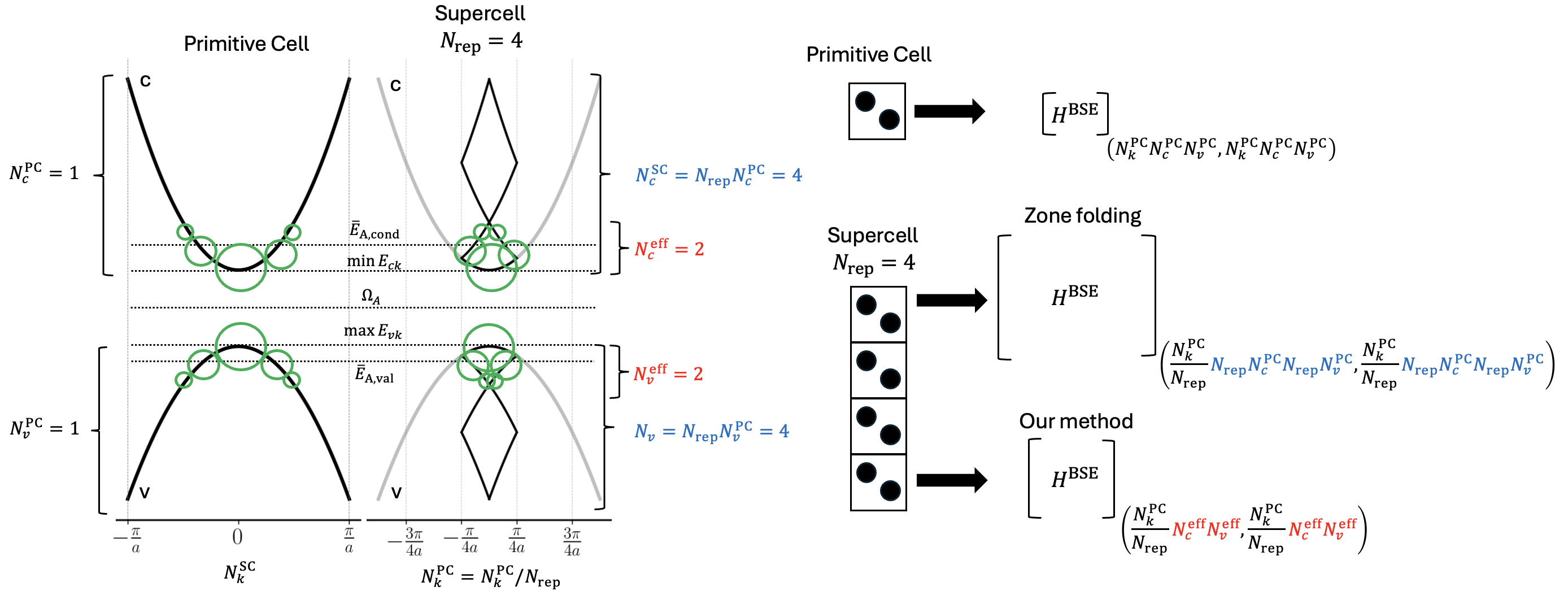
Figure 1: Diagram showing zone folding of the bandstructure and exciton coefficient. We show a 1D example of bands being zone folded in a BZ of a SC four times the size of the PC. Circle radius is proportional to $|A_{kcv}|$. For the PC calculation, only one valence and one conduction band is necessary to converge this exciton wavefunction. For the SC, just two valence and two conduction bands are necessary to represent this exciton, not four as would be expected by a zone folding analysis. $\bar{E}_{A,\rm{cond(val)}}$ are given by equation 2.

III Computational Details

We used ONCV scalar-relativistic LDA pseudopotentials with standard precision from pseudodojo website [45, 46]. Parameters for DFT calculations: $E_{\rm{cut}}=80\rm{Ry}$ and a regular $k$-grid = $4\times 4\times 4$ for PC calculations. We use the experimental lattice parameter at 300K that is 4.026 Å [47, 48, 49]. For GW/BSE calculations: coarse and fine grids are $4\times 4\times 4$, then no interpolation from coarse to fine grids is done. The cutoff energy to build the dielectric matrix is 20 Ry. We performed G₀W₀ calculations within Generalized Plasmon Pole [20, 17] using the stochastic pseudobands method [21] with an accumulation window of 2%, 2 stochastic pseudobands per energy subspcace, and generating empty states with energy up to the DFT cutoff (80 Ry). The PC BSE Hamiltonian is built with 5 valence and 10 conduction bands.

The SC is composed of $4\times 4\times 4$ PCs and has 128 atoms. For a faithful comparison both PC and SC have LiF in the rocksalt structure, and our objective in this example is to make SC calculations reproduce results from the PC case, therefore both coarse and fine $k$-grids include only the $\Gamma$-point. Except for the number of conduction and valence states to build the BSE Hamiltonian, all other GW/BSE and DFT parameters are the same as in the PC case.

DFT calculations were performed with the Quantum ESPRESSO code [50, 51, 52] (version 7.2) and GW/BSE calculations were performed with BerkeleyGW code [20, 18, 17] (version 4.0), but this approach is general and can be used by other codes that solve BSE.

IV Results

To test this approach we show results for rocksalt LiF. For comparison we show in figure 2 the density of states (DOS) for the SC and PC calculations at DFT and QP levels. The two curves for both DFT and QP DOS are almost identical. For the PC case, we find a GW gap of 14.502 eV while for SC the bandgap is 14.550 (see table 2). The difference of 48 meV, which is 0.3% of the PC gap is due to approximations used in stochastic pseudobands method [21].

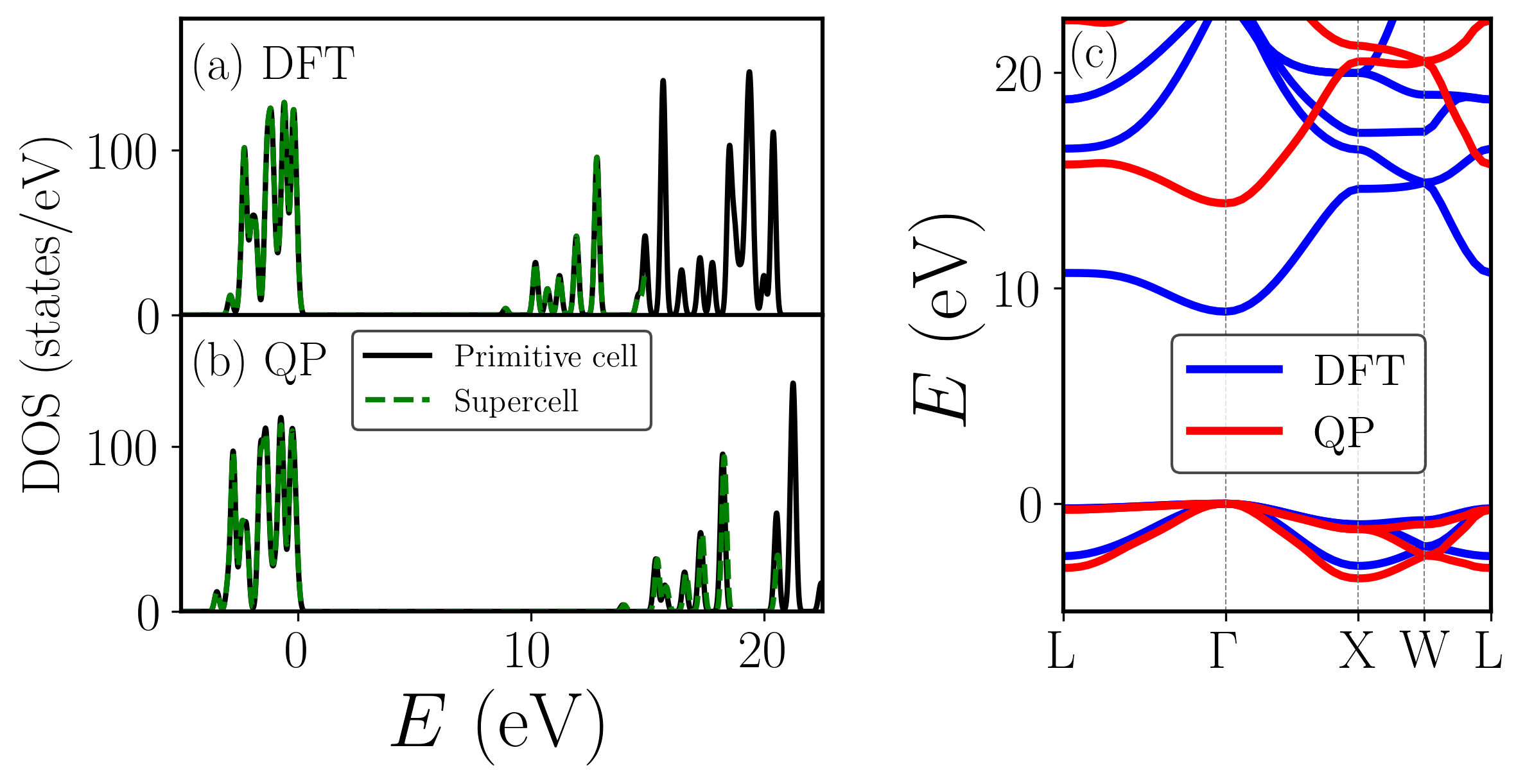
Figure 2: Density of States (DOS) at DFT (a) and QP (b) levels for rocksalt LiF calculations in a 2-atoms PC (black solid lines) and a 128-atoms SC (green dashed lines). Direct bandgap energies at the $\Gamma$-point are reported in Table 2. For DOS calculation a Gaussian broadening of 0.1 eV was used. (c) DFT and QP bandstructure of LiF, from PC.

Then we calculate the exciton energies for PC LiF using a $4\times 4\times 4$ $k$-grid, five valence bands, and ten conduction bands to build the BSE Hamiltonian. Due to the Brillouin zone folding, just the $\Gamma$ point is necessary for BSE calculations for the SC. Zone folding also predicts 320 valence and 640 conduction bands. To choose a reasonable number of bands, we show $\bar{E}^{QP}_{A,\rm{val}}$ and $\bar{E}^{QP}_{A,\rm{cond}}$ for several excitons on figure 3. We note that WASPE increases as exciton energies get higher. Valence band energies vary less than conduction, as the bandwidth of the conduction band for LiF is larger than for the valence band (see Figure 2). To build a proper BSE Hamiltonian for SC calculations we decided to include states that are relevant to excitons with energy up to 17 eV, which means including all conduction states with energy up to 4 eV above the minimum of the conduction band and all valence states 2 eV below the maximum of the valence band. In this case, this means to include 137 valence and 31 conduction bands, which is 2% of the size of a BSE Hamiltonian given by zone folding. Even in the case of approximately considering for PC just one conduction and the three first (degenerate at $\Gamma$) valence bands, which compose the first bright exciton in LiF the BSE Hamiltonian size is 35% of the size of the BSE Hamiltonian created from zone folding, saving computational resources substantially.

Figure 3: Energy analysis for excitons with energy ranging 11.7 to 20.0 eV. (a) Small dots are the WASPE (equation 2) for excitons with excitation energy $\Omega$. Circles are the energies of the states that compose the exciton, where the color grading is proportional to $|A_{kcv}|^{2}$, showing the distribution in energy of the states that compose this exciton. (b) Same as (a) but for valence states. (c) QP bandstructure for PC around $\Gamma$ point. The green line is the excitation energy of the first exciton, and red (blue) dashed line is the weighted average conduction (valence) single-particle energy (see equation 2 and text) for the first bright exciton (first absorption peak on figure 4). Green, red, and blue dotted lines are the same as dashed lines but for the second bright exciton (second absorption peaks on figure 4).

It is important to stress that an analysis based only on converging QP energy levels would lead to inaccurate conclusions. One could neglect the electron-hole interaction and use the Random Phase Approximation (RPA) with QP energy levels. Naively, the absorption spectra looks like the one obtained by solving the BSE but blueshifted (see figure 4(a)). On figure 4(b) we show that the first two RPA peaks energies converge faster than the exciton energies.

V Discussion

Next, we show the optical absorption spectra for PC and SC cases in figure 4. We observed that for energies up to 17 eV absorption peaks for SC are blueshifted by 0.2 eV in relation to PC results (see table 2), while no absorption peak is present for energies above 17 eV. This was expected as we determined $\bar{E}^{QP}_{A,\rm{val}}$ to include all states of excitons with energy up to 17 eV. On the right side of figure 4 we plot the energy of the first exciton as a function of the BSE Hamiltonian size. The smaller the BSE Hamiltonian size is, the larger the deviation from the PC results (black dashed lines).

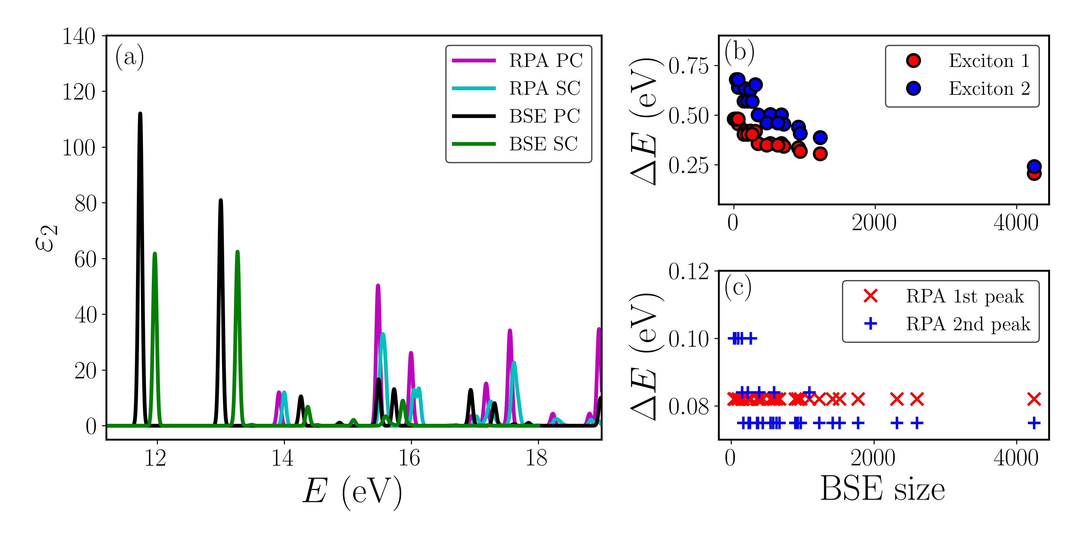
Figure 4: (a) Optical absorption for PC and SC cases calculated at BSE and RPA (not including excitonic effects) levels. For the SC we used 137 valence and 31 conduction states to build the BSE Hamiltonian. Absorption peaks from SC calculations are blueshifted by $\sim 0.2$ eV. (b) Convergence with respect to PC results of first (red) and second (blue) exciton energies in SC BSE calculations as a function of the BSE Hamiltonian size. In (c) we show the convergence of the first and second peak energies calculated at RPA level.

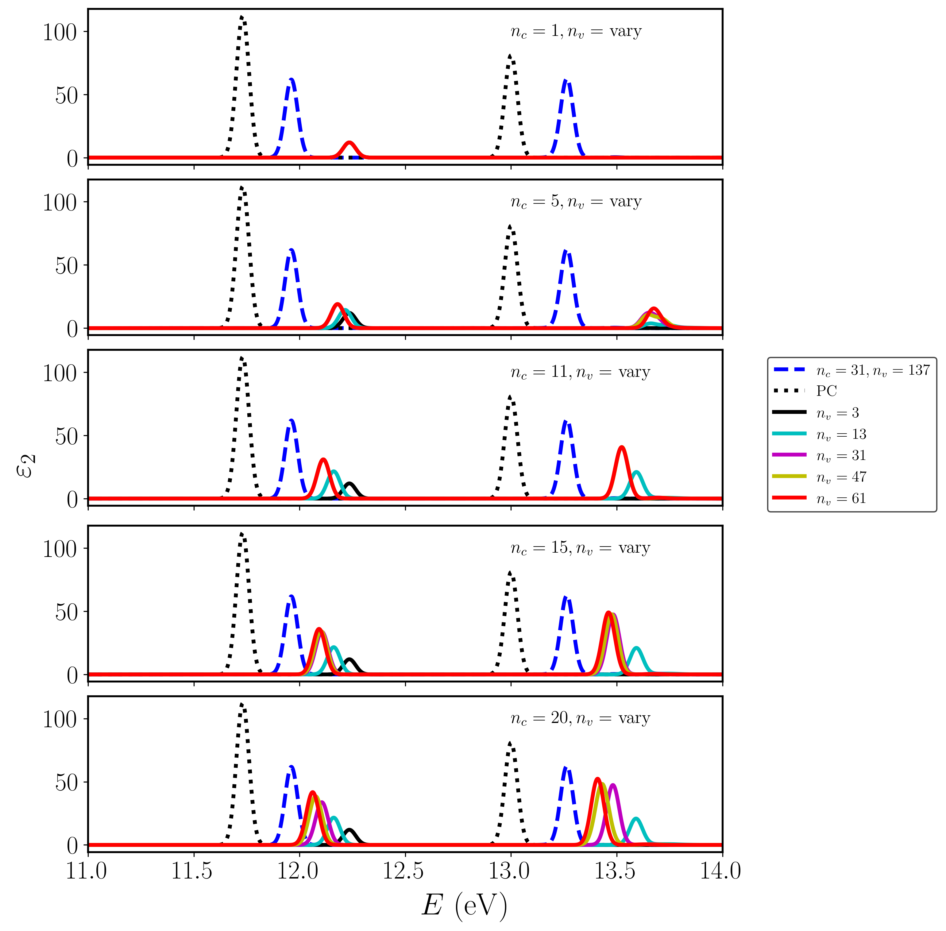
Figure 5: Optical absorption varying the number of conduction and valence bands in the BSE Hamiltonian.

	This work		Other works
Energies (eV)	PC	SC	Theory	Experiment
DFT Gap at $\Gamma$	8.8723	8.8756	8.91 [9]
QP Gap at $\Gamma$	14.502	14.550	14.4 [18], 14.3 [9], 14.5 [29]	$14.2\pm 0.2$ [53]
$\Omega_{1}$	12.368		12.8 [18], 12.7 [9], 12.82 [29]	12.5 [54]
$\Omega_{2}$	13.851
$E_{b1}$	2.134		1.6 [18], 1.88 [29]
$E_{b2}$	0.921

Table 2: Exciton energies for first ($\Omega_{1}$) and second ($\Omega_{2}$) absorption peaks (see Figure 4) for calculations in SC and PC.

One important aspect to be considered is that due to zone-folding, finite-momentum excitons of PC may be folded into the SC results. To illustrate it we show in figure 6 the joint density of states (JDOS) of SC calculations and compare it with the PC case. For a fair comparison the PC BSE results must include finite-momentum excitons that will be folded into the SC Brillouin Zone. Our finite momentum results include excitons with momentum $Q$ [55], where $Q$ is a k-vector of a regular $4\times 4\times 4$ grid. As we increased the number of bands to build the BSE Hamiltonian the JDOS gets closer to PC results with finite momentum excitons. PC JDOS with just excitons with $Q=0$ ($\Gamma$ point) is zero in the region between 12.3 and 13.0 eV, but in our SC result the JDOS is finite in agreement with PC JDOS using excitons with finite momentum. Finite momentum excitons are dark as photons carry no momentum, and here we are comparing PC and SC calculations for the same RS structure, so the optical absorption for the two cases is almost identical. Although one may be studying cases where there is a symmetry breaking in the SC case (e.g. a point defect), which can brighten those dark excitons, so a well converged JDOS is also necessary. In figure 6, we show how the JDOS of the SC evolves when increasing the BSE size and our choice with 137 valence and 31 conduction bands agrees well with PC JDOS with excitons with finite $Q$.

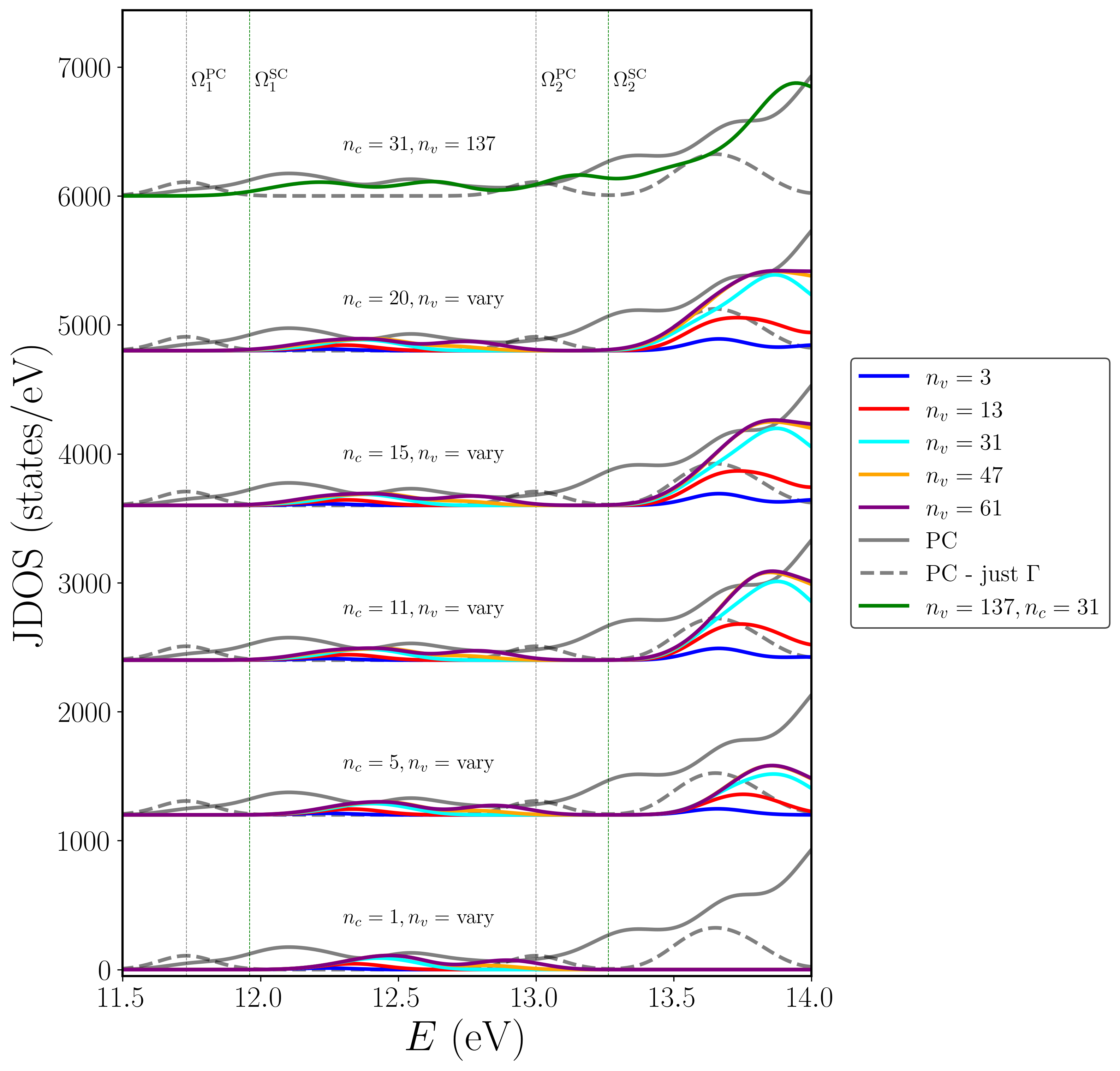
Figure 6: Joint Density of States (Exciton Density of States) for PC calculations (gray full and dashed lines) compared with SC calculations with different numbers of conduction and valence states to build the BSE Hamiltonian. We show two PC calculations, one where just excitons with zero center of mass momentum are included in the calculation (gray dashed lines) and the other where all excitons with finite momentum $Q$ from a regular grid $4\times 4\times 4$ are included (gray dashed lines). Due to the zone folding a BSE calculation for SC will also present excitons with finite momentum of PC. The more bands are used to build the BSE Hamiltonian the closer the SC exciton DOS gets to PC exciton DOS. Vertical lines are the energies of the first and second bright excitons (see table 2).

VI Conclusions

We presented in this paper a proper scheme to set the Hamiltonian size for SC calculations based on PC results without the need for new convergence studies. The expected single-particle energies of each exciton provide a window of states that need to be included in the SC BSE Hamiltonian. This also allows one to choose for which energy levels GW calculations are necessary, avoiding unnecessary calculations and make SC GW/BSE calculations more accessible. This method may be applied to study the optical properties of surfaces, defects, and polarons in diverse materials and speed-up ab initio results of excitons calculations.

References

- Del Ben et al. [2019] M. Del Ben, F. H. da Jornada, A. Canning, N. Wichmann, K. Raman, R. Sasanka, C. Yang, S. G. Louie, and J. Deslippe, Large-scale GW calculations on pre-exascale HPC systems, Comput. Phys. Commun. 235, 187–195 (2019).
- Anh Pham et al. [2013] T. Anh Pham, T. Li, H.-V. Nguyen, S. Shankar, F. Gygi, and G. Galli, Band offsets and dielectric properties of the amorphous Si3N4/Si(100) interface: A first-principles study, Appl. Phys. Lett. 102, 241603 (2013).
- Strubbe et al. [2015] D. A. Strubbe, E. C. Johlin, T. R. Kirkpatrick, T. Buonassisi, and J. C. Grossman, Stress effects on the raman spectrum of an amorphous material: Theory and experiment on -Si:H, Phys. Rev. B 92, 241202 (2015).
- Winkler et al. [2017] B. Winkler, L. Martin-Samos, N. Richard, L. Giacomazzi, A. Alessi, S. Girard, A. Boukenter, Y. Ouerdane, and M. Valant, Correlations between structural and optical properties of peroxy bridges from first principles, J. Phys. Chem. C 121, 4002–4010 (2017).
- Ismail-Beigi and Louie [2005] S. Ismail-Beigi and S. G. Louie, Self-trapped excitons in silicon dioxide: Mechanism and properties, Phys. Rev. Lett. 95 (2005).
- Del Grande and Strubbe [2025] R. R. Del Grande and D. A. Strubbe, Revisiting ab-initio excited state forces from many-body Green’s function formalism: approximations and benchmark (2025), arXiv:2502.05144 [cond-mat.mtrl-sci] .
- Cook and Beran [2020] C. Cook and G. J. O. Beran, Reduced-cost supercell approach for computing accurate phonon density of states in organic crystals, J. Chem. Phys. 153, 224105 (2020).
- Franchini et al. [2021] C. Franchini, M. Reticcioli, M. Setvin, and U. Diebold, Polarons in materials, Nature Rev. Mater. 6, 560–586 (2021).
- Wang et al. [2003] N.-P. Wang, M. Rohlfing, P. Krüger, and J. Pollmann, Quasiparticle band structure and optical spectrum of LiF(001), Phys. Rev. B 67, 115111 (2003).
- Freysoldt et al. [2014] C. Freysoldt, B. Grabowski, T. Hickel, J. Neugebauer, G. Kresse, A. Janotti, and C. G. Van de Walle, First-principles calculations for point defects in solids, Rev. Mod. Phys. 86, 253 (2014).
- Shim et al. [2005] J. Shim, E.-K. Lee, Y. J. Lee, and R. M. Nieminen, Density-functional calculations of defect formation energies using supercell methods: Defects in diamond, Phys. Rev. B 71, 035206 (2005).
- Castleton et al. [2009] C. W. M. Castleton, A. Höglund, and S. Mirbt, Density functional theory calculations of defect energies using supercells, Model. Simul. Mater. Sci. Eng. 17, 084003 (2009).
- Abtew et al. [2011] T. A. Abtew, Y. Y. Sun, B.-C. Shih, P. Dev, S. B. Zhang, and P. Zhang, Dynamic Jahn-Teller effect in the center in diamond, Phys. Rev. Lett. 107, 146403 (2011).
- Barker and Strubbe [2022] B. A. Barker and D. A. Strubbe, Spin-flip Bethe-Salpeter equation approach for ground and excited states of open-shell molecules and defects in solids (2022), arXiv:2207.04549 [cond-mat.mtrl-sci] .
- Lischner et al. [2012] J. Lischner, J. Deslippe, M. Jain, and S. G. Louie, First-principles calculations of quasiparticle excitations of open-shell condensed matter systems, Phys. Rev. Lett. 109, 036406 (2012).
- Ma et al. [2010] Y. Ma, M. Rohlfing, and A. Gali, Excited states of the negatively charged nitrogen-vacancy color center in diamond, Phys. Rev. B 81, 041204 (2010).
- Hybertsen and Louie [1986] M. S. Hybertsen and S. G. Louie, Electron correlation in semiconductors and insulators: Band gaps and quasiparticle energies, Phys. Rev. B 34, 5390 (1986).
- Rohlfing and Louie [2000] M. Rohlfing and S. G. Louie, Electron-hole excitations and optical spectra from first principles, Phys. Rev. B 62, 4927 (2000).
- Payne et al. [1992] M. C. Payne, M. P. Teter, D. C. Allan, T. A. Arias, and J. D. Joannopoulos, Iterative minimization techniques for ab initio total-energy calculations: molecular dynamics and conjugate gradients, Rev. Mod. Phys. 64, 1045 (1992).
- Deslippe et al. [2012] J. Deslippe, G. Samsonidze, D. A. Strubbe, M. Jain, M. L. Cohen, and S. G. Louie, BerkeleyGW: A massively parallel computer package for the calculation of the quasiparticle and optical properties of materials and nanostructures, Comput. Phys. Commun. 183, 1269 (2012).
- Altman et al. [2024] A. R. Altman, S. Kundu, and F. H. da Jornada, Mixed stochastic-deterministic approach for many-body perturbation theory calculations, Phys. Rev. Lett. 132, 086401 (2024).
- Forde et al. [2023] A. Forde, S. Tretiak, and A. J. Neukirch, Dielectric screening and charge-transfer in 2D lead-halide perovskites for reduced exciton binding energies, Nano Lett. 23, 11586–11592 (2023).
- Trolle et al. [2017] M. L. Trolle, T. G. Pedersen, and V. Véniard, Model dielectric function for 2D semiconductors including substrate screening, Sci. Rep. 7, 39844 (2017).
- Peelaers et al. [2011] H. Peelaers, B. Partoens, M. Giantomassi, T. Rangel, E. Goossens, G.-M. Rignanese, X. Gonze, and F. M. Peeters, Convergence of quasiparticle band structures of Si and Ge nanowires in the approximation and the validity of scissor shifts, Phys. Rev. B 83, 045306 (2011).
- da Jornada et al. [2017] F. H. da Jornada, D. Y. Qiu, and S. G. Louie, Nonuniform sampling schemes of the Brillouin zone for many-electron perturbation-theory calculations in reduced dimensionality, Phys. Rev. B 95, 035109 (2017).
- Strubbe [2012] D. A. Strubbe, Optical and Transport Properties of Organic Molecules: Methods and Applications., Ph.D. thesis, University of California, Berkeley (2012).
- Naik et al. [2022] M. H. Naik, E. C. Regan, Z. Zhang, Y.-H. Chan, Z. Li, D. Wang, Y. Yoon, C. S. Ong, W. Zhao, S. Zhao, M. I. B. Utama, B. Gao, X. Wei, M. Sayyad, K. Yumigeta, K. Watanabe, T. Taniguchi, S. Tongay, F. H. da Jornada, F. Wang, and S. G. Louie, Intralayer charge-transfer moiré excitons in van der waals superlattices, Nature 609, 52–57 (2022).
- Susarla et al. [2022] S. Susarla, M. H. Naik, D. D. Blach, J. Zipfel, T. Taniguchi, K. Watanabe, L. Huang, R. Ramesh, F. H. da Jornada, S. G. Louie, P. Ercius, and A. Raja, Hyperspectral imaging of exciton confinement within a moiré unit cell with a subnanometer electron probe, Science 378, 1235–1239 (2022).
- Dai et al. [2024a] Z. Dai, C. Lian, J. Lafuente-Bartolome, and F. Giustino, Theory of excitonic polarons: From models to first-principles calculations, Phys. Rev. B 109, 045202 (2024a).
- Dai et al. [2024b] Z. Dai, C. Lian, J. Lafuente-Bartolome, and F. Giustino, Excitonic polarons and self-trapped excitons from first-principles exciton-phonon couplings, Phys. Rev. Lett. 132, 036902 (2024b).
- Zanfrognini et al. [2023] M. Zanfrognini, N. Spallanzani, M. Bonacci, E. Molinari, A. Ruini, M. J. Caldas, A. Ferretti, and D. Varsano, Effect of uniaxial strain on the excitonic properties of monolayer C3N: A symmetry-based analysis, Phys. Rev. B 107, 045430 (2023).
- Cho and Berkelbach [2019] Y. Cho and T. C. Berkelbach, Optical properties of layered hybrid organic–inorganic halide perovskites: A tight-binding GW-BSE study, J. Phys. Chem. Lett. 10, 6189–6196 (2019).
- Bieniek et al. [2022] M. Bieniek, K. Sadecka, L. Szulakowska, and P. Hawrylak, Theory of excitons in atomically thin semiconductors: Tight-binding approach, Nanomaterials 12, 1582 (2022).
- Dias et al. [2023] A. C. Dias, J. F. Silveira, and F. Qu, Wantibexos: A Wannier based tight binding code for electronic band structure, excitonic and optoelectronic properties of solids, Comput. Phys. Commun. 285, 108636 (2023).
- Sio et al. [2019a] W. H. Sio, C. Verdi, S. Poncé, and F. Giustino, Polarons from first principles, without supercells, Phys. Rev. Lett. 122, 246403 (2019a).
- Sio et al. [2019b] W. H. Sio, C. Verdi, S. Poncé, and F. Giustino, Ab initio theory of polarons: Formalism and applications, Phys. Rev. B 99, 235139 (2019b).
- Baldacchini et al. [2001] G. Baldacchini, R. Montereali, and T. Tsuboi, Energy transfer among color centers in LiF crystals, Eur. Phys. J. D. 17, 261–264 (2001).
- Shluger et al. [1991] A. L. Shluger, N. Itoh, V. E. Puchin, and E. N. Heifets, Two types of self-trapped excitons in alkali halide crystals, Phys. Rev. B 44, 1499 (1991).
- Song and Baetzold [1992] K. S. Song and R. C. Baetzold, Structure of the self-trapped exciton and nascent Frenkel pair in alkali halides: An ab initio study, Phys. Rev. B 46, 1960 (1992).
- Martin [2004] R. M. Martin, Electronic Structure: Basic Theory and Practical Methods (Cambridge University Press, 2004).
- Qiu et al. [2021] D. Y. Qiu, F. H. da Jornada, and S. G. Louie, Solving the Bethe-Salpeter equation on a subspace: Approximations and consequences for low-dimensional materials, Phys. Rev. B 103, 045117 (2021).
- Stanzione et al. [2020] D. Stanzione, J. West, R. T. Evans, T. Minyard, O. Ghattas, and D. K. Panda, Frontera: The evolution of leadership computing at the National Science Foundation, in Practice and Experience in Advanced Research Computing 2020: Catch the Wave, PEARC ’20 (Association for Computing Machinery, New York, NY, USA, 2020) p. 106–111.
- Sun et al. [2022] M. Sun, M. Re Fiorentin, U. Schwingenschlögl, and M. Palummo, Excitons and light-emission in semiconducting MoSi2X4 two-dimensional materials, npj 2D Mater. Appl. 6 (2022).
- Dadkhah and Lambrecht [2024] N. Dadkhah and W. R. L. Lambrecht, Band structure and excitonic properties of in the isolated monolayer limit in an all-electron approach, Phys. Rev. B 109, 195155 (2024).
- van Setten et al. [2018] M. van Setten, M. Giantomassi, E. Bousquet, M. Verstraete, D. Hamann, X. Gonze, and G.-M. Rignanese, The pseudodojo: Training and grading a 85 element optimized norm-conserving pseudopotential table, Comput. Phys. Commun. 226, 39 (2018).
- Hamann [2013] D. R. Hamann, Optimized norm-conserving Vanderbilt pseudopotentials, Phys. Rev. B 88, 085117 (2013).
- Ben Yahia et al. [2012] H. Ben Yahia, M. Shikano, H. Sakaebe, S. Koike, M. Tabuchi, H. Kobayashi, H. Kawaji, M. Avdeev, W. Miiller, and C. D. Ling, Synthesis and characterization of the crystal structure, the magnetic and the electrochemical properties of the new fluorophosphate LiNaFe[PO4]F, Dalton Trans. 41, 11692 (2012).
- Srivastava and Merchant [1973] K. Srivastava and H. Merchant, Thermal expansion of alkali halides above 300°K, J. Phys. Chem. Solids. 34, 2069–2073 (1973).
- Shadike et al. [2021] Z. Shadike, H. Lee, O. Borodin, X. Cao, X. Fan, X. Wang, R. Lin, S.-M. Bak, S. Ghose, K. Xu, C. Wang, J. Liu, J. Xiao, X.-Q. Yang, and E. Hu, Identification of LiH and nanocrystalline LiF in the solid–electrolyte interphase of lithium metal anodes, Nat. Nanotechnol. 16, 549–554 (2021).
- Giannozzi et al. [2009] P. Giannozzi, S. Baroni, N. Bonini, M. Calandra, R. Car, C. Cavazzoni, D. Ceresoli, G. L. Chiarotti, M. Cococcioni, I. Dabo, A. D. Corso, S. de Gironcoli, S. Fabris, G. Fratesi, R. Gebauer, U. Gerstmann, C. Gougoussis, A. Kokalj, M. Lazzeri, L. Martin-Samos, N. Marzari, F. Mauri, R. Mazzarello, S. Paolini, A. Pasquarello, L. Paulatto, C. Sbraccia, S. Scandolo, G. Sclauzero, A. P. Seitsonen, A. Smogunov, P. Umari, and R. M. Wentzcovitch, QUANTUM ESPRESSO: a modular and open-source software project for quantum simulations of materials, J. Phys.: Condens. Matter 21, 395502 (2009).
- Giannozzi et al. [2017] P. Giannozzi, O. Andreussi, T. Brumme, O. Bunau, M. B. Nardelli, M. Calandra, R. Car, C. Cavazzoni, D. Ceresoli, M. Cococcioni, N. Colonna, I. Carnimeo, A. D. Corso, S. de Gironcoli, P. Delugas, R. A. DiStasio, A. Ferretti, A. Floris, G. Fratesi, G. Fugallo, R. Gebauer, U. Gerstmann, F. Giustino, T. Gorni, J. Jia, M. Kawamura, H.-Y. Ko, A. Kokalj, E. Küçükbenli, M. Lazzeri, M. Marsili, N. Marzari, F. Mauri, N. L. Nguyen, H.-V. Nguyen, A. O. de-la Roza, L. Paulatto, S. Poncé, D. Rocca, R. Sabatini, B. Santra, M. Schlipf, A. P. Seitsonen, A. Smogunov, I. Timrov, T. Thonhauser, P. Umari, N. Vast, X. Wu, and S. Baroni, Advanced capabilities for materials modelling with quantum ESPRESSO, J. Phys.: Condens. Matter 29, 465901 (2017).
- Giannozzi et al. [2020] P. Giannozzi, O. Baseggio, P. Bonfà, D. Brunato, R. Car, I. Carnimeo, C. Cavazzoni, S. de Gironcoli, P. Delugas, F. F. Ruffino, A. Ferretti, N. Marzari, I. Timrov, A. Urru, and S. Baroni, Quantum Espresso toward the exascale, J. Chem. Phys. 152, 154105 (2020).
- Piacentini et al. [1976] M. Piacentini, D. W. Lynch, and C. G. Olson, Thermoreflectance of LiF between 12 and 30 eV, Phys. Rev. B 13, 5530 (1976).
- Roessler and Walker [1967] D. M. Roessler and W. C. Walker, Optical constants of magnesium oxide and lithium fluoride in the far ultraviolet, J. Opt. Soc. Am. 57, 835 (1967).
- Qiu et al. [2015] D. Y. Qiu, T. Cao, and S. G. Louie, Nonanalyticity, valley quantum phases, and lightlike exciton dispersion in monolayer transition metal dichalcogenides: Theory and first-principles calculations, Phys. Rev. Lett. 115, 176801 (2015).