Error estimates for viscous Burgers’ equation using deep learning method

Abstract.

The articles focuses on error estimates as well as stability analysis of deep learning methods for stationary and non-stationary viscous Burgers equation in two and three dimensions. The local well-posedness of homogeneous boundary value problem for non-stationary viscous Burgers equation is established by using semigroup techniques and fixed point arguments. By considering a suitable approximate problem and deriving appropriate energy estimates, we prove the existence of a unique strong solution. Additionally, we extend our analysis to the global well-posedness of the non-homogeneous problem. For both the stationary and non-stationary cases, we derive explicit error estimates in suitable Lebesgue and Sobolev norms by optimizing a loss function in a Deep Neural Network approximation of the solution with fixed complexity. Finally, numerical results on prototype systems are presented to illustrate the derived error estimates.

Keywords. Deep Neural Networks $\cdot$ Viscous Burgers equation $\cdot$ Error estimates $\cdot$ Non-homogeneous boundary value problems $\cdot$ PINNs.
MSC Classification (2020). 65N15 $\cdot$ 68T07 $\cdot$ 35A01 $\cdot$ 35A02.

1. Introduction

The Burgers equation is a fundamental partial differential equation (PDE) that arises in various fields, including fluid dynamics, gas dynamics, traffic flow, and turbulence modeling. Serving as a simplified model for the more complex Navier-Stokes equations, it provides valuable insights into nonlinear advection-diffusion processes. The study of the Burgers equation in two and three dimensions is essential for understanding diffusion-driven wave dynamics, shock formation, and wavefront propagation which are key phenomena in real-world physical systems.

1.1. Motivation

There are various numerical methods for solving PDEs, including the finite difference method, finite element method, and finite volume method. However, these traditional approaches often come with limitations, such as high computational cost and long execution times. In recent years, machine learning methods, particularly deep neural networks (DNNs), have shown promise in addressing these challenges. Among these, Physics-Informed Neural Networks (PINNs) [27] have gained significant attention for solving PDEs efficiently. One of the key advantages of PINNs is their ability to approximate a PDE’s solution without requiring a discretized grid. This is achieved by training a neural network to satisfy both the PDE and the associated boundary/initial conditions.

Deep learning [12] is a branch of machine learning that focuses on developing models inspired by the structure and functioning of the human brain. It builds on artificial neural networks to create systems capable of interpreting and learning from data. Multi-layer perceptrons, which consist of multiple hidden layers, are commonly used in deep learning. Figure 1 provides an illustration of a four-layer neural network used for the PINN approximation of Burgers equation. In this setup, the network is supervised, meaning it requires a “teacher” to guide it by providing the desired outputs. The system constructs high-level representations by combining simpler, lower-level features, forming more abstract concepts. This hierarchical architecture consists of an input layer, several hidden layers, and an output layer, with connections existing only between neighboring layers. Each layer can act as a logistic regression model, enabling the network to develop complex concepts from simpler building blocks, making deep learning a powerful and flexible tool for data interpretation.

A typical dense neural network computes layer-by-layer transformations for a given input $x$:

$$y_{2}(x)=\sigma(W_{1}x+b_{1}),\quad y_{3}(y_{2})=\sigma(W_{2}y_{2}+b_{2}),\dots$$

leading to the final output:

$$u_{\theta}(x)=y_{n+1}(y_{n}(\dots y_{2}(x))).$$

Here, $\theta=\{W_{1},W_{2},\dots,W_{n},b_{1},\dots,b_{n}\}$ represents all the weights and biases, and $\sigma$ is a nonlinear activation function and $n$ denote the number of layers. The objective of neural network training is to “learn” or optimize the parameters $\theta$ by minimizing a chosen loss function.

Our goal in this paper is not to exhaustively analyze all possible neural network architectures for solving PDEs. Instead, we focus on providing a mathematically rigorous analysis of the PINN approximated solution, including error estimates and stability analysis, in the context of solving viscous Burgers equations in two and three dimensions. Our approach is similar in spirit to the probabilistic error analysis for machine learning algorithms applied to the Black-Scholes equations [4]. Specifically, we consider two different settings: the stationary case, which serves to establish fundamental ideas and illustrate our methodology, and the non-stationary case, which is the primary focus of this work. A detailed summary of our key contributions is provided in Section 1.3.

Figure 1. An illustration of the PINN algorithm for solving a PDE, with the loss function specifically formulated for the Burgers equation.

1.2. Literature survey

Given the extensive applications of the Burgers equation, numerous numerical methods have been developed to solve it. The finite element method, in particular, has been widely utilized, as documented in studies such as [2, 5, 26, 20, 8, 7] and references therein. Error estimates for the one-dimensional Burgers equation were derived and verified through numerical experiments in [26]. The study in [20] provides an optimal error estimate accompanied by a comprehensive numerical analysis for the one-dimensional case. Additionally, [7] applied a weak Galerkin finite element method to achieve optimal-order error estimates for the one-dimensional Burgers equation, examining both semi-discrete and fully discrete systems, with numerical verification provided.

The finite element method is a standard approach for solving PDEs, while the success of deep neural networks in various approximation tasks has led to the development of PINNs for this purpose. PINNs and their variants have shown strong capabilities in approximating a wide range of PDEs. However, to date, PINNs and the finite element method have primarily been explored independently [11, 25]. There are vast literature available where PINN is used to solve partial differential equations, for example, see [4, 30, 31, 29, 27], and references their in. The work [30] established error bounds for ReLU neural network approximations of parametric hyperbolic scalar conservation laws, including generalization error bounds based on training error, sample size, and network size. The authors in [29] provided error bounds for approximating the incompressible Navier-Stokes equations with PINN, proving that the residual error can be minimized with $\tanh$ networks, and that total error depends on training error, network size, and quadrature points.

1.3. Contributions

In this article, in addition to deriving error estimates, we establish the explicit solvability of both stationary and non-stationary viscous Burgers equations with homogeneous and non-homogeneous boundary data.

One of the key contributions of this work is the extension of existing DNN approximation results to Sobolev spaces. Specifically, in Theorem 2.8, we establish that for any function in the Sobolev space $H^{m}(\Omega)\cap H^{1}_{0}(\Omega)$, there exists a NN that approximates it with arbitrarily small error in the Sobolev norm. This result extends and generalizes a prior approximation theorem [33, Theorem 3.3], originally formulated for $C^{k}$ functions, to a broader Sobolev space setting. By leveraging the density of smooth, compactly supported functions in Sobolev spaces and applying known DNN approximation result, we rigorously prove that NNs can approximate Sobolev functions with controlled accuracy. This theoretical finding provides a solid foundation for the application of deep learning methods in solving PDE, ensuring that the learned solutions retain both accuracy and regularity in the Sobolev norm.

In Section 3, we begin by analyzing the stationary viscous Burgers equation, establishing the well-posedness of weak and strong solutions for the homogeneous boundary data case using Brouwer’s fixed-point theorem and the Faedo-Galerkin method. Building upon this, in Theorem 3.3, we address the existence and uniqueness of weak and strong solutions for non-homogeneous boundary data through a lifting argument, providing explicit results. These results are essential for the subsequent error estimates in deep learning approximation.

To rigorously assess the accuracy of these approximations, we first analyze the impact of boundary data errors. When the boundary data error is $L^{2}$, we show that if the residual error is of order $\varepsilon$ , then the corresponding error in the solution is of order $\varepsilon^{2/3}$, demonstrating the reliability of deep learning approaches for solving PDEs with quantified error bounds. Furthermore, by considering boundary data in $H^{1/2}$, we establish that the solution error can be improved back to the original order of $\varepsilon$ (Theorem 3.4). Additionally, in Theorem 3.6, we prove that a neural network solution exists for the stationary viscous Burgers equation, where both the residual error and the solution error can be made arbitrarily small. This analysis underscores the crucial role of boundary regularity in error control and confirms that deep learning techniques provide reliable approximations with precise error characterization in stationary PDE settings.

For the non-stationary viscous Burgers equation, in Section 4, we establish the existence and uniqueness of strong solutions with homogeneous boundary conditions in both two and three dimensions using a fixed-point argument combined with an approximation method. Theorem 4.3 proves the local existence of solutions on $[0,T^{*}]$ for some $0<T^{*}<T$ which is then extended to a global solution in Theorem 4.6, covering the entire time interval $[0,T].$ Furthermore, in Theorem 4.8, we employ a lifting argument—solving an associated non-homogeneous heat equation, to establish the existence and uniqueness of both weak and strong solutions under non-homogeneous boundary conditions. These results lay the groundwork for our subsequent error estimate analysis.

To extend our error analysis to time-dependent solutions using deep learning methods, in Section 5, we establish error estimates similar to those in the stationary case, demonstrating the robustness of our approach in dynamic scenarios. Specifically, Theorem 5.1 shows that if the residual error is of order $\varepsilon$, then the solution error is of order $\varepsilon$. In Theorem 5.2, we extend the results of Theorem 3.6 to the non-stationary case, proving that a DNN solution exists where both the residual error and solution error can be made arbitrarily small. Additionally, Theorem 5.4 presents a stability analysis, demonstrating that two DNN solutions remain“close enough” when their respective input data are “close enough”. These findings highlight the adaptability of deep learning-based methods in capturing both spatial and temporal variations in PDE solutions.

Finally, in Section 6, we present numerical experiments for both the stationary and non-stationary cases to illustrate our theoretical findings. These examples demonstrate the effectiveness of the deep learning approach in approximating solutions while showing that the derived error bounds hold as expected.

The remainder of this article is organized as follows. Section 2 introduces the functional setting and key inequalities used throughout the paper, concluding with a key result on the existence of a deep neural network approximation in Sobolev spaces with arbitrarily small error.

2. Functional setting and mathematical framework

We provide the function spaces needed to obtain the required results and some basic inequalities in this section.

2.1. Functional setting

Let $\Omega$ be a bounded domain in $\mathbb{R}^{d}$. Let $C_{c}^{\infty}(\Omega)$ be the space of all $C^{\infty}$ functions with compact support contained in $\Omega$. For $1\leq p<\infty,$ let $L^{p}(\Omega)$ denote the space of equivalence classes of Lebesgue measurable functions $f:\Omega\to\mathbb{R}$ such that $\int_{\Omega}|f(x)|^{p}dx<\infty$, where two measurable functions are equivalent if they are equal a.e. For $f\in L^{p}(\Omega)$, we define the $L^{p}-$norm of $f$ as $\|f\|_{L^{p}(\Omega)}:=\left(\int_{\Omega}|f(x)|^{p}dx\right)^{1/p}$. We define $L^{\infty}(\Omega)$, the equivalence class of Lebesgue measurable functions $f:\Omega\to\mathbb{R}$ for which $\|f\|_{L^{\infty}(\Omega)}:=\mathrm{ess\ sup}_{x\in\Omega}|f(x)|<\infty$. For $p=2$, $L^{2}(\Omega)$ is a Hilbert space and the inner product in $L^{2}(\Omega)$ is denoted by $(\cdot,\cdot)$ and is given by $(f,g)=\int_{\Omega}f(x)g(x)dx$, and the corresponding norm is denoted by $\|\cdot\|$. Moreover, let $H_{0}^{1}(\Omega)$ denote the Sobolev space (also denoted as $W^{1,2}_{0}(\Omega)$), which is defined as the space of equivalence classes of Lebesgue measurable functions $f\in L^{2}(\Omega)$ such that its weak derivative $\nabla f\in L^{2}(\Omega)$ and $f$ is of trace zero. The $H_{0}^{1}(\Omega)-$norm is defined by $\|{f}\|_{H_{0}^{1}(\Omega)}:=\left(\int_{\Omega}|\nabla f(x)|^{2}dx\right)^{1/2}$ (by using the Poincaré inequality). Then, we define $H^{-1}(\Omega):=(H_{0}^{1}(\Omega))^{\prime}$, that is, dual of the Sobolev space $H_{0}^{1}(\Omega)$, with norm

$$\|{g}\|_{H^{-1}(\Omega)}:=\sup\left\{{\langle g,f\rangle}:f\in H_{0}^{1}(\Omega),\ {\|{f}\|_{H_{0}^{1}(\Omega)}}\leq 1\right\},$$

where $\langle\cdot,\cdot\rangle$ represent the duality pairing between $H_{0}^{1}(\Omega)$ and $H^{-1}(\Omega)$. We denote the second order Hilbertian Sobolev spaces by $H^{2}(\Omega)$. The general Sobolev spaces will be denoted by $W^{m,p}(\Omega)$, where $m\in\mathbb{N}$ and $p\in[1,\infty)$. It is known that there exists a linear continuous operator $\gamma_{0}\in\mathcal{L}(H^{1}(\Omega),L^{2}(\Gamma))$ (the trace operator), such that $\gamma_{0}u$ equals the restriction of $u$ to $\Gamma,$ for every function $u\in H^{1}(\Omega)$ which is twice continuously differentiable in $\overline{\Omega}$, see [32, p. 9]. The kernel of $\gamma_{0}$ is equivalent to the space $H_{0}^{1}(\Omega)$. The image space $\gamma_{0}(H^{1}(\Omega))$ is a dense subspace of $L^{2}(\Gamma)$, which is represented by $H^{1/2}(\Gamma)$, that is,

$$H^{1/2}(\Gamma)=\gamma_{0}(H^{1}(\Omega))=\{v\in L^{2}(\Gamma):\text{ there exists a }u\in H^{1}(\Omega)\mbox{ such that }\gamma_{0}(u)=v\}.$$

The space $H^{1/2}(\Gamma)$ can be equipped with the norm carried from $H^{1}(\Omega)$ by $\gamma_{0}$. The dual space of $H^{1/2}(\Gamma)$ is denoted by $H^{-1/2}(\Gamma)$. Moreover, there exists a linear continuous operator $\ell_{\Omega}\in\mathcal{L}(H^{1/2}(\Gamma),H^{1}(\Omega))$, which is called a lifting operator, such that $\gamma_{0}\circ\ell_{\Omega}=$ the identity operator in $H^{1/2}(\Gamma)$. Similarly, one can define $H^{3/2}(\Gamma)=\gamma_{0}(H^{2}(\Omega))$. For further information, see Lions $\&$ Magenes [17] and McLean [21].

The norm in any space $X$ is denoted by $\|\cdot\|_{X}.$ The constant $C>0$ is generic and may depend on the given parameters, and domain.

2.2. Some useful inequalities

We recall some useful inequalities that is used in the paper frequently.

Young’s inequality. Let $a,b$ be any non-negative real numbers. Then for any $\varepsilon>0,$ the following inequalities hold:

$$ab\leq\frac{\varepsilon a^{2}}{2}+\frac{b^{2}}{2\varepsilon}\text{ and }ab\leq\frac{a^{p}}{p}+\frac{b^{q}}{q},$$ (2.1)

for any $p,q>1$ such that $\frac{1}{p}+\frac{1}{q}=1.$

Proposition 2.1 (Generalized Hölder’s inequality).

Let $\Omega$ be a bounded domain in $\mathbb{R}^{d}$. Let $f\in L^{p}(\Omega),$ $g\in L^{q}(\Omega),$ and $h\in L^{r}(\Omega),$ where $1\leq p,q,r\leq\infty$ are such that $\frac{1}{p}+\frac{1}{q}+\frac{1}{r}=1.$ Then $fgh\in L^{1}(\Omega)$ and

$$\|fgh\|_{L^{1}(\Omega)}\leq\|f\|_{L^{p}(\Omega)}\|g\|_{L^{q}(\Omega)}\|h\|_{L^{r}(\Omega)}.$$

Lemma 2.2 (Agmons’ inequality [1]).

Let $\Omega$ be a bounded domain in $\mathbb{R}^{d},\,d\in\{1,2,3\},$ and let $f\in H^{s_{2}}(\Omega).$ Let $s_{1},s_{2}$ be such that $s_{1}<\frac{d}{2}<s_{2}.$ If for $0<\theta<1,$ $\frac{d}{2}=\theta s_{1}+(1-\theta)s_{2},$ then there exists a positive constant $C_{a}=C_{a}(\Omega)$ such that

$$\|f\|_{L^{\infty}(\Omega)}\leq C_{a}\|f\|_{H^{s_{1}}(\Omega)}^{\theta}\|f\|_{H^{s_{2}}(\Omega)}^{1-\theta}.$$ (2.2)

In the following lemma, we recall Sobolev embedding [14, Theorem 2.4.4] in our context.

Lemma 2.3 (Sobolev embedding).

Let $\Omega$ be a bounded domain in $\mathbb{R}^{d}$ of class $C^{1}$ with $d\in\mathbb{N}.$ Then, we have the following continuous embedding with constant $C_{s}$:

• $H^{1}(\Omega)\hookrightarrow L^{p}(\Omega)$ for $d>2,$ where $p=\frac{2d}{d-2},$

• $H^{1}(\Omega)\hookrightarrow L^{q}(\Omega)$ for all $d=2\leq q<\infty.$

In the next theorem, we recall the important inequality, known as the Gagliardo-Nirenberg inequality in the case of bounded domain with smooth boundary.

Theorem 2.4 (Gagliardo-Nirenberg inequality [24]).

Let $\Omega\subset\mathbb{R}^{d},$ $d\in\{2,3\},$ be a convex domain or domain with $C^{2}$-boundary $\Gamma$. For any $u\in W^{m,q}(\Omega)$, and for any integers $j$ and $m$ satisfying $0\leq j<m$, the following inequality holds:

$$\|D^{j}u\|_{L^{p}(\Omega)}\leq C\|u\|_{W^{m,q}(\Omega)}^{\theta}\|u\|_{L^{r}(\Omega)}^{1-\theta},$$

where $D^{j}u$ denotes the $j$-th order weak derivative of $u$, and:

$$\frac{1}{p}=\frac{j}{d}+\theta\left(\frac{1}{q}-\frac{m}{d}\right)+\frac{(1-\theta)}{r},$$

for some constant $C$ that depends on the domain $\Omega$ but not on $u$, where $\theta\in[0,1]$.

Lemma 2.5 (General Gronwall inequality [6]).

Let $f,g,h$ and $y$ be four locally integrable positive functions on $[t_{0},\infty)$ such that

$$y(t)+\int_{t_{0}}^{t}f(s)ds\leq C+\int_{t_{0}}^{t}h(s)ds+\int_{t_{0}}^{t}g(s)y(s)ds\ \text{ for all }t\geq t_{0},$$

where $C\geq 0$ is any constant. Then

$$y(t)+\int_{t_{0}}^{t}f(s)ds\leq\left(C+\int_{t_{0}}^{t}h(s)ds\right)\exp\left(\int_{t_{0}}^{t}g(s)ds\right)\text{ for all }t\geq t_{0}.$$

Now, we state a version of nonlinear generalization of Gronwalls’ inequality that will be useful in our later analysis.

Theorem 2.6.

(A nonlinear generalization of Gronwall’s inequality [9, Theorem 21]). Let $\zeta(t)$ be a non-negative locally integrable function that satisfies the integral inequality

$$\zeta(t)\leq c+\int_{t_{0}}^{t}\left(a(s)\zeta(s)+b(s)\zeta^{\varepsilon}(s)\right)ds,c\geq 0,\ 0\leq\varepsilon<1,$$

where $a(t)$ and $b(t)$ are continuous non-negative functions for $t\geq t_{0}.$ Then, the following inequality holds:

$$\zeta(t)\leq\left\{c^{1-\varepsilon}\exp{\left[(1-\varepsilon)\int_{t_{0}}^{t}a(s)ds\right]}+(1-\varepsilon)\int_{t_{0}}^{t}b(s)\exp{\left[(1-\varepsilon)\int_{s}^{t}a(r)dr\right]}ds\right\}^{\frac{1}{1-\varepsilon}}.$$

2.3. Approximation using DNN

The aim of this section is to show that for a given function in a suitable Sobolev space, we can find a suitable function in DNN so that they are “close enough” in the Sobolev norm. In particular, we want to extend the result in [33, Theorem 3.3], which is stated below, to Sobolev spaces.

Theorem 2.7 ([33, Theorem 3.3]).

Let $\sigma\in C^{\infty}(\mathbb{R})$ with $\sigma^{(n)}\neq 0$ for all $n=1,2,3,\ldots,$ and $K\subset\mathbb{R}^{d}$ be any compact set. Then for any $f\in C^{k}(K)$, $k\in\mathbb{N}$, a function $\phi_{N}$ represented by a Deep Neural Network with complexity $N\in\mathbb{N}$ exists such that

$$\|D^{\alpha}f-D^{\alpha}\phi_{N}\|_{C(K)}=O\left(\frac{1}{N^{\frac{k-|\alpha|}{d}}}\,\sup_{x,y\in K,|x-y|\leq\frac{1}{N^{1/d}}}|D^{\beta}f(x)-D^{\beta}f(y)|\right)$$

holds for all multi-indices $\alpha,\beta$ with $|\alpha|\leq k,\ |\beta|=k.$

Here, we extend the above result in the Sobolev space $H^{m}(\Omega)$ as follows:

Theorem 2.8.

Let $\Omega\subset\mathbb{R}^{d},$ $d\in\{2,3\},$ be a convex domain or domain with $C^{2}$-boundary $\Gamma,$ and $f\in H^{m}(\Omega)\cap H^{1}_{0}(\Omega)$ for any $m=1,2,\ldots.$ Let $\varepsilon>0$ be given. Then a function $\phi_{N}$ represented by a Deep Neural Network with complexity $N\in\mathbb{N}$ exists such that

$$\|f-\phi_{N}\|_{H^{m}(\Omega)}\leq\varepsilon.$$

Proof.

Recall that $C^{\infty}_{c}(\Omega)$ is dense in $H^{m}(\Omega)\cap H^{1}_{0}(\Omega)$ and therefore for given $\varepsilon>0,$ there exists $g\in C^{\infty}_{c}(\Omega)$ such that $\|f-g\|_{H^{m}(\Omega)}\leq\frac{\varepsilon}{2}.$

Since $g\in C^{\infty}_{c}(\Omega),$ there exists compact set $\mathcal{K}\subset\Omega$ such that

$$\text{supp}(g)\subset\mathcal{K},\,D^{\alpha}g=0\text{ in }\Omega\backslash\mathcal{K}\text{ for all multiindices }\alpha.$$

Let us fix $K=\overline{\Omega}$ in Theorem 2.7. Note that $\mathcal{K}\subset\Omega\subset K$ and since, $g\in C^{k}(K)$ for all $k=1,2,\ldots,$ one can apply Theorem 2.7 for $g.$ Let $\alpha$ be any multiindex such that $|\alpha|\leq m.$ Then from Theorem 2.7, we can find a $\phi_{N}$ represented by a DNN such that

$$\sup_{x\in K}|D^{\alpha}g(x)-D^{\alpha}\phi_{N}(x)|\leq C\frac{1}{N^{\frac{m-|\alpha|+1}{d}}}.$$

Further note that

$$\int_{K}|(D^{\alpha}g(x)-D^{\alpha}\phi_{N}(x))|^{2}dx\leq\sup_{x\in K}|D^{\alpha}g(x)-D^{\alpha}\phi_{N}(x)|^{2}|\Omega|\leq C\frac{1}{N^{\frac{2(m-|\alpha|+1)}{d}}}|\Omega|.$$

Now, choosing suitable large $N$, we obtain

$$\|g-\phi_{N}\|_{H^{m}(K)}\leq\frac{\varepsilon}{2}.$$

Therefore,

$$\|f-\phi_{N}\|_{H^{m}(\Omega)}\leq\|f-g\|_{H^{m}(\Omega)}+\|g-\phi_{N}\|_{H^{m}(\Omega)}\leq\varepsilon,$$

which is completes the proof. ∎

3. Error estimates for stationary viscous Burgers equation

The main objective of this section is to establish error estimates for stationary viscous Burgers’ equation using deep learning method. Let $\Omega\subset\mathbb{R}^{d},$ $d\in\{2,3\},$ be a convex domain or domain with $C^{2}$-boundary $\Gamma$. We first consider the following stationary viscous Burgers equation:

$$\left\{\begin{aligned} &-\nu\Delta u_{\infty}(x)+\sum_{i=1}^{d}u_{\infty}(x)\frac{\partial u_{\infty}}{\partial x_{i}}(x)=f_{\infty}(x)\ \text{ in }\ \Omega,\\ &u_{\infty}(x)=0\ \text{ on }\ \Gamma,\end{aligned}\right.$$ (3.1)

where $\nu>0$ is a given constant and $f_{\infty}$ is the forcing term. The explicit function space for $f_{\infty}$ is stated in the following theorem. Now, we state a result on the existence and uniqueness of weak as well as strong solutions of (3.1).

Theorem 3.1 ([23]).

For given $f\in H^{-1}(\Omega),$ there exists a weak solution (of (3.1)) $u_{\infty}\in H^{1}_{0}(\Omega)$ such that

$$\|u_{\infty}\|_{H^{1}(\Omega)}\leq\frac{1}{\nu}\|f_{\infty}\|_{H^{-1}(\Omega)}.$$

If $f_{\infty}\in L^{2}(\Omega),$ then $u_{\infty}\in H^{2}(\Omega)\cap H^{1}_{0}(\Omega)$ and satisfies

$$\|u_{\infty}\|_{H^{2}(\Omega)}\leq C(\nu)\|f_{\infty}\|.$$

Moreover, if

$$\nu>\left\{\begin{array}[]{cc}\left(\frac{2}{\lambda_{1}}\right)^{1/4}\|f_{\infty}\|_{H^{-1}(\Omega)}&\ \text{ if }d=2,\\ \left(\frac{\sqrt{2}}{\lambda_{1}^{1/8}}\right)\|f_{\infty}\|_{H^{-1}(\Omega)}&\ \text{ if }d=3,\end{array}\right.$$ (3.4)

where $\lambda_{1}$ is the first eigenvalue of Dirichlet’s Laplacian, then the weak solution is unique.

By using Brouwer’s fixed-point theorem ([32, Chapter 2, Section 1]) and a Galerkin approximation method, one can establish the proof of above theorem and is standard (for example, see [15, Theorems 2.1 - 2.3]), hence we omit here.

Remark 3.2.

The condition (3.4) means that one has to take $\nu$ sufficiently large for arbitrary external forcing $f_{\infty}\in H^{-1}(\Omega)$ and small external forcing for arbitrary $\nu>0$.

Now, we briefly discuss the existence of a strong solution for the following stationary viscous Burgers equation with non-homogeneous boundary data, which is helpful in the sequel:

$$\left\{\begin{aligned} &-\nu\Delta u_{\infty}(x)+\sum_{i=1}^{d}u_{\infty}(x)\frac{\partial u_{\infty}}{\partial x_{i}}(x)=f_{\infty}(x)\ \text{ in }\ \Omega,\\ &u_{\infty}(x)=g_{\infty}(x)\ \text{ on }\ \Gamma.\end{aligned}\right.$$ (3.5)

Theorem 3.3.

For a given $f_{\infty}\in H^{-1}(\Omega)$ and $g_{\infty}\in H^{\frac{1}{2}}(\Gamma),$ there exists a weak solution $u_{\infty}\in H^{1}(\Omega)$ of (3.5) satisfying

$$\|u_{\infty}\|_{H^{1}(\Omega)}\leq C\left(\|f_{\infty}\|_{H^{-1}(\Omega)}+\|g_{\infty}\|_{H^{\frac{1}{2}}(\Gamma)}\right),$$

for some $C>0.$

For $f_{\infty}\in L^{2}(\Omega)$ and $g_{\infty}\in H^{\frac{3}{2}}(\Gamma),$ every weak solution of (3.5) is a strong solution $u_{\infty}\in H^{2}(\Omega)$ satisfying

$$\|u_{\infty}\|_{H^{2}(\Omega)}\leq C\left(\|f_{\infty}\|+\|g_{\infty}\|_{H^{\frac{3}{2}}(\Gamma)}\right),$$

for some $C>0.$ Moreover, if $\nu>0$ is sufficiently large, then the solution is unique.

Proof.

For a given $g_{\infty}\in H^{s+\frac{1}{2}}(\Gamma),$ $s\in\{0,1\}$, one can define a lifting operator $\ell:H^{s+\frac{1}{2}}(\Gamma)\rightarrow H^{1+s}(\Omega)$ and let $z:=\ell(g_{\infty}).$ We also have

$$\|z\|_{H^{1+s}(\Omega)}\leq C_{\ell}\|g\|_{H^{s+\frac{1}{2}}(\Gamma)},\ s\in\{0,1\}.$$ (3.6)

Then $v:=u_{\infty}-z$ satisfies

$$\left\{\begin{aligned} &-\nu\Delta v+\sum_{i=1}^{d}v\frac{\partial v}{\partial x_{i}}+\sum_{i=1}^{d}v\frac{\partial z}{\partial x_{i}}+\sum_{i=1}^{d}\frac{\partial v}{\partial x_{i}}z=f_{\infty}+\nu\Delta z-\sum_{i=1}^{d}z\frac{\partial z}{\partial x_{i}}\text{ in }\Omega,\\ &v=0\text{ on }\Gamma.\end{aligned}\right.$$ (3.7)

For $g_{\infty}\in H^{\frac{1}{2}}(\Gamma)$ and $f_{\infty}\in H^{-1}(\Omega)$, one can show that

$$\bigg{\|}f_{\infty}+\nu\Delta z-\frac{1}{2}\sum_{i=1}^{d}\frac{\partial z^{2}}{\partial x_{i}}\bigg{\|}_{H^{-1}(\Omega)} \leq\|f_{\infty}\|_{H^{-1}(\Omega)}+\nu\|z\|_{H^{1}(\Omega)}+C\|z\|_{L^{4}(\Omega)}^{2}$$

$$\leq\|f_{\infty}\|_{H^{-1}(\Omega)}+C_{\ell}\|g\|_{H^{\frac{1}{2}}(\Gamma)}+C_{s}\|z\|_{H^{1}(\Omega)}^{2}$$

$$\leq\|f_{\infty}\|_{H^{-1}(\Omega)}+C\|g\|_{H^{\frac{1}{2}}(\Gamma)}+C\|g\|_{H^{\frac{1}{2}}(\Gamma)}^{2},$$

where we have used Sobolev’s inequality and (3.6). Then by using similar arguments as in the proof of [15, Theorems 2.22 - 2.2] (see Theorem 3.1), one can obtain the existence of a weak solution to the problem (3.7).

For $g_{\infty}\in H^{\frac{3}{2}}(\Gamma)$ and $f_{\infty}\in L^{2}(\Omega)$, it is immediate that

$$\bigg{\|}f_{\infty}+\nu\Delta z-\sum_{i=1}^{d}z\frac{\partial z}{\partial x_{i}}\bigg{\|} \leq\|f_{\infty}\|+\nu\|z\|_{H^{2}(\Omega)}+\|z\|_{L^{4}(\Omega)}\|\nabla z\|_{L^{4}(\Omega)}$$

$$\leq\|f_{\infty}\|+\nu C_{\ell}\|g_{\infty}\|_{H^{\frac{3}{2}}(\Gamma)}+C_{s}C_{\ell}\|g_{\infty}\|_{H^{\frac{3}{2}}(\Gamma)}^{2},$$

where once again we have used Sobolev’s inequality and (3.6). Now, following a similar argument as in the proof of [15, Theorem 2.3] (Theorem 3.1), one can show that the weak solution is strong and $v\in H^{2}(\Omega)\cap H^{1}_{0}(\Omega)$ of (3.7). Therefore, since $u_{\infty}=v+z$, the problem (3.5) admits unique weak solution for sufficiently large $\nu$, $f_{\infty}\in H^{-1}(\Omega)$ and $g_{\infty}\in H^{\frac{1}{2}}(\Gamma),$ and a strong solution for $f_{\infty}\in L^{2}(\Omega),g_{\infty}\in H^{\frac{3}{2}}(\Gamma)$. ∎

3.1. Minimization problem

To discuss the error estimates for stationary viscous Burgers equation using deep learning method, it is convenient to consider the following minimization problem ([4]):

$$\inf_{u_{\infty}\in\text{appropriate space}}\bigg{\{}\Big{\|}-\nu\Delta u_{\infty}+\sum_{i=1}^{d}u_{\infty}\frac{\partial u_{\infty}}{\partial x_{i}}-f_{\infty}\Big{\|}^{2}+\|u_{\infty}|_{\Gamma}\|^{2}_{L^{2}(\Gamma)}\bigg{\}},$$

and it has a unique solution, with the value of the infimum being zero and the infimum is attained at the solution $u_{\infty}$ of (3.1). Thus, in order to approximate $u_{\infty}$ using a DNN, one considers the following loss function:

$$\Big{\|}-\nu\Delta u_{\infty}^{N}+\sum_{i=1}^{d}u_{\infty}^{N}\frac{\partial u_{\infty}^{N}}{\partial x_{i}}-f_{\infty}\Big{\|}^{2}+ \|u_{\infty}^{N}|_{\Gamma}\|^{2}_{L^{2}(\Gamma)},\ u_{\infty}^{N}\in\mathcal{F}_{N},$$

under the restriction that $u_{\infty}^{N}$ is bounded in $H^{2}(\Omega)$. More precisely, let $p_{k}\in\Omega$ for $k=1,2,\ldots,m$ and $q_{j}\in\Gamma$ for $j=1,2,\ldots,n$ be some chosen points. Then on these points, we write the cost functional as

$$\inf_{\{\tilde{u}^{N}\in\mathcal{F}_{N},\ \|\tilde{u}^{N}\|_{H^{2}(\Omega)}\leq M\}}\sum_{k=1}^{m}\bigg{|}-\nu\Delta\tilde{u}^{N}(p_{k})+\sum_{i=1}^{d}\tilde{u}^{N}(p_{k})\frac{\partial\tilde{u}^{N}}{\partial x_{i}}(p_{k})-f_{\infty}(p_{k})\bigg{|}^{2}+\sum_{j=1}^{n}|\tilde{u}^{N}(q_{j})|^{2}.$$

3.2. Error estimates

In the next theorem, we show that if there is a DNN $u_{\infty}^{N}$ that approximates (3.1), then it is “close enough” to $u_{\infty},$ the exact solution of (3.1).

Theorem 3.4.

Let $f_{\infty}\in L^{2}(\Omega)$ and $u_{\infty}$ be the solution of stationary Burgers equation (3.1), and for a given $\varepsilon>0$, there exists $u_{\infty}^{N}\in\mathcal{F}_{N}$ with $\|u_{\infty}^{N}\|_{H^{2}(\Omega)}\leq M$ such that

$$\Big{\|}-\nu\Delta u_{\infty}^{N}+\sum_{i=1}^{d}u_{\infty}^{N}\frac{\partial u_{\infty}^{N}}{\partial x_{i}}-f_{\infty}\Big{\|}^{2}+\|\left.u_{\infty}^{N}\right|_{\Gamma}\|_{L^{2}(\Gamma)}^{2}\leq\varepsilon^{2}.$$ (3.8)

Then for

$$\nu>\max\left\{\sqrt{3}\left(\frac{1}{2\lambda_{1}}\right)^{1/4}\|f_{\infty}\|_{H^{-1}(\Omega)}^{1/2},\frac{3}{2}C_{\ell}M\varepsilon^{2/3}\right\}$$ (3.9)

and for some $C>0,$ the following estimate holds:

$$\|u_{\infty}-u_{\infty}^{N}\|_{H^{1}(\Omega)}\leq C\varepsilon^{\frac{2}{3}}.$$

Furthermore, under the assumption

$$\Big{\|}-\nu\Delta u_{\infty}^{N}+\sum_{i=1}^{d}u_{\infty}^{N}\frac{\partial u_{\infty}^{N}}{\partial x_{i}}-f_{\infty}\Big{\|}^{2}+\|\left.u_{\infty}^{N}\right|_{\Gamma}\|_{H^{1/2}(\Gamma)}^{2}\leq\varepsilon^{2},$$ (3.10)

we obtain the improved estimate as

$$\|u_{\infty}-u_{\infty}^{N}\|_{H^{1}(\Omega)}\leq\varepsilon.$$

Proof.

Let $\displaystyle-\widetilde{f}_{\infty}:=-\nu\Delta u_{\infty}^{N}+\sum_{i=1}^{d}u_{\infty}^{N}\frac{\partial u_{\infty}^{N}}{\partial x_{i}}-f_{\infty}$ and $-\widetilde{g}_{\infty}:=\left.u_{\infty}^{N}\right|_{\Gamma}.$ Then $u_{\infty}^{N}$ satisfies

$$\left\{\begin{aligned} &-\nu\Delta u_{\infty}^{N}+\sum_{i=1}^{d}u_{\infty}^{N}\frac{\partial u_{\infty}^{N}}{\partial x_{i}}=f_{\infty}-\widetilde{f}_{\infty}\text{ in }\Omega,\\ &u_{\infty}^{N}=-\widetilde{g}_{\infty}\text{ on }\Gamma.\end{aligned}\right.$$

Set $w=u_{\infty}-u_{\infty}^{N}$ to obtain

$$\left\{\begin{aligned} &-\nu\Delta w+\sum_{i=1}^{d}(u_{\infty}-u_{\infty}^{N})\frac{\partial u_{\infty}}{\partial x_{i}}+\sum_{i=1}^{d}u_{\infty}^{N}\frac{\partial}{\partial x_{i}}(u_{\infty}-u_{\infty}^{N})=\widetilde{f}_{\infty}\text{ in }\Omega,\\ &w=\widetilde{g}_{\infty}\text{ on }\Gamma,\end{aligned}\right.$$

which further can be re-written as

$$\left\{\begin{aligned} &-\nu\Delta w+\sum_{i=1}^{d}w\frac{\partial u_{\infty}}{\partial x_{i}}+\sum_{i=1}^{d}u_{\infty}\frac{\partial w}{\partial x_{i}}-\sum_{i=1}^{d}w\frac{\partial w}{\partial x_{i}}=\widetilde{f}_{\infty}\text{ in }\Omega,\\ &w=\widetilde{g}_{\infty}\text{ on }\Gamma.\end{aligned}\right.$$ (3.11)

The solvability of the above problem is discussed in Theorem 3.3. Consider the lifting operator $\ell:H^{1/2}(\Gamma)\rightarrow H^{1}(\Omega)$ and denote $z:=\ell(\widetilde{g}_{\infty}).$ Then $z$ and $\widetilde{g}_{\infty}$ satisfy ([17, 21])

$$\|z\|_{H^{1}(\Omega)}\leq C_{\ell}\|\widetilde{g}_{\infty}\|_{H^{1/2}(\Gamma)}.$$ (3.12)

Now, set $v=w-z,$ so that we have

$$\left\{\begin{aligned} &-\nu\Delta(v+z)+\sum_{i=1}^{d}(v+z)\frac{\partial u_{\infty}}{\partial x_{i}}+\sum_{i=1}^{d}u_{\infty}\frac{\partial}{\partial x_{i}}(v+z)-\sum_{i=1}^{d}(v+z)\frac{\partial}{\partial x_{i}}(v+z)=\widetilde{f}_{\infty}\text{ in }\Omega,\\ &v=0\text{ on }\Gamma.\end{aligned}\right.$$

On simplifying this, we obtain

$$\left\{\begin{aligned} &-\nu\Delta v+\sum_{i=1}^{d}v\frac{\partial u_{\infty}}{\partial x_{i}}+\sum_{i=1}^{d}z\frac{\partial u_{\infty}}{\partial x_{i}}+\sum_{i=1}^{d}u_{\infty}\frac{\partial v}{\partial x_{i}}+\sum_{i=1}^{d}u_{\infty}\frac{\partial z}{\partial x_{i}}\\ &\qquad\qquad-\sum_{i=1}^{d}v\frac{\partial v}{\partial x_{i}}-\sum_{i=1}^{d}v\frac{\partial z}{\partial x_{i}}-\sum_{i=1}^{d}z\frac{\partial v}{\partial x_{i}}=\widetilde{f}_{\infty}+\nu\Delta z+\sum_{i=1}^{d}z\frac{\partial z}{\partial x_{i}}\text{ in }\Omega,\\ &v=0\text{ on }\Gamma.\end{aligned}\right.$$

Taking the inner product with $v$ leads to

$$\nu\|\nabla v\|^{2} =-\Big{(}\sum_{i=1}^{d}v\frac{\partial u_{\infty}}{\partial x_{i}},v\Big{)}-\Big{(}\sum_{i=1}^{d}u_{\infty}\frac{\partial v}{\partial x_{i}},v\Big{)}-\Big{(}\sum_{i=1}^{d}z\frac{\partial u_{\infty}}{\partial x_{i}},v\Big{)}-\Big{(}\sum_{i=1}^{d}u_{\infty}\frac{\partial z}{\partial x_{i}},v\Big{)}$$ (3.13)

$$\quad+\Big{(}\sum_{i=1}^{d}v\frac{\partial z}{\partial x_{i}},v\Big{)}+\Big{(}\sum_{i=1}^{d}z\frac{\partial v}{\partial x_{i}},v\Big{)}+(\widetilde{f}_{\infty},v)-\nu(\nabla z,\nabla v)+\Big{(}\sum_{i=1}^{d}z\frac{\partial z}{\partial x_{i}},v\Big{)}$$

$$=\Big{(}\sum_{i=1}^{d}u_{\infty}\frac{\partial v}{\partial x_{i}},v\Big{)}+\Big{(}\sum_{i=1}^{d}\frac{\partial v}{\partial x_{i}},u_{\infty}z\Big{)}+\frac{1}{2}\Big{(}\sum_{i=1}^{d}v\frac{\partial z}{\partial x_{i}},v\Big{)}-\frac{1}{2}\Big{(}\sum_{i=1}^{d}z\frac{\partial v}{\partial x_{i}},z\Big{)}$$

$$\qquad+(\widetilde{f}_{\infty},v)-\nu(\nabla z,\nabla v)$$

$$=\sum_{k=1}^{6}I_{k},$$

where we have performed integration by parts. Using Hölder’s, Ladyzhenskaya’s and Poincaré’s inequalities, and Theorem 3.1, we estimate $I_{1}$ as

$$|I_{1}| =\Big{|}\Big{(}\frac{1}{2}\sum_{i=1}^{d}v\frac{\partial u_{\infty}}{\partial x_{i}},v\Big{)}\Big{|}\leq\frac{1}{2}\|\nabla u_{\infty}\|\|v\|_{L^{4}(\Omega)}^{2}\leq\frac{1}{\sqrt{2}}\|\nabla u_{\infty}\|\|\nabla v\|\|v\|\leq\sqrt{\frac{1}{2\lambda_{1}}}\|\nabla u_{\infty}\|\|\nabla v\|^{2}$$

$$\leq\frac{1}{\nu}\sqrt{\frac{1}{2\lambda_{1}}}\|f_{\infty}\|_{H^{-1}(\Omega)}\|\nabla v\|^{2}.$$

A generalized Hölder’s inequality, (3.12), and Theorem 3.1 lead to

$$|I_{2}| =\Big{|}\Big{(}\sum_{i=1}^{d}\frac{\partial v}{\partial x_{i}},u_{\infty}z\Big{)}\Big{|}\leq\|\nabla v\|\|u_{\infty}\|_{L^{4}(\Omega)}\|z\|_{L^{4}(\Omega)}\leq\frac{\eta\nu}{4}\|\nabla v\|^{2}+C\|z\|_{H^{1}(\Omega)}^{2}\|u_{\infty}\|_{H^{1}(\Omega)}^{2}$$

$$\leq\frac{\eta\nu}{4}\|\nabla v\|^{2}+C\|f_{\infty}\|_{H^{-1}(\Omega)}^{2}\|\widetilde{g}_{\infty}\|_{H^{1/2}(\Gamma)}^{2},$$

where the constant $C$ depends on $C_{s},\nu,$ and $C_{\ell},$ and the constant $\eta>0$ which will be specified later. Using generalized Hölder’s inequality, Sobolev’s embedding and (3.12), we obtain

$$|I_{3}|=\Big{|}\frac{1}{2}\Big{(}\sum_{i=1}^{d}v\frac{\partial z}{\partial x_{i}},v\Big{)}\Big{|}\leq\frac{1}{2}\|\nabla z\|\|v\|_{L^{4}(\Omega)}^{2}\leq\frac{1}{2}\|z\|_{H^{1}(\Omega)}\|\nabla v\|^{2}\leq\frac{C_{\ell}}{2}\|\widetilde{g}_{\infty}\|_{H^{1/2}(\Gamma)}\|\nabla v\|^{2}.$$

Once again applying generalized Hölder’s and Cauchy Schwarz inequalities, and (3.12), we deduce

$$|I_{4}|=\Big{|}\frac{1}{2}\Big{(}\sum_{i=1}^{d}z\frac{\partial v}{\partial x_{i}},z\Big{)}\Big{|}\leq\frac{1}{2}\|\nabla v\|\|z\|_{L^{4}(\Omega)}^{2}\leq\frac{\eta\nu}{4}\|\nabla v\|^{2}+C\|\widetilde{g}_{\infty}\|_{H^{1/2}(\Gamma)}^{4},$$

where the constant $C$ depends on $C_{s},\nu,$ and $C_{\ell}.$ Hölder’s and Young’s inequalities yield

$$|I_{5}| =|(\widetilde{f}_{\infty},v)|\leq\frac{\eta\nu}{4}\|\nabla v\|^{2}+C_{\nu}\|\widetilde{f}_{\infty}\|^{2}_{H^{-1}(\Omega)},$$

$$|I_{6}| =|\nu(\nabla z,\nabla v)|\leq\frac{\eta\nu}{4}\|\nabla v\|^{2}+C_{\nu}\|\nabla z\|^{2}\leq\frac{\eta\nu}{4}\|\nabla v\|^{2}+C\|\widetilde{g}_{\infty}\|_{H^{1/2}(\Gamma)}^{2}.$$

For the given hypothesis (3.8), we use interpolation and Trace theories to find

$$\|\widetilde{g}_{\infty}\|_{H^{\frac{1}{2}}(\Gamma)}\leq\|\widetilde{g}_{\infty}\|_{L^{2}(\Gamma)}^{\frac{2}{3}}\|\widetilde{g}_{\infty}\|_{H^{\frac{3}{2}}(\Gamma)}^{\frac{1}{3}}\leq\varepsilon^{\frac{2}{3}}\|u_{\infty}^{N}\|_{H^{2}(\Omega)}^{\frac{1}{3}}\leq M\varepsilon^{\frac{2}{3}}.$$

Moreover, using (3.8), we also have

$$\|\widetilde{f}_{\infty}\|_{H^{-1}(\Omega)}\leq\varepsilon.$$

Let $\eta=\frac{1}{3}.$ Now, one can choose $\nu$ sufficiently large or $\|f_{\infty}\|_{H^{-1}(\Omega)}$ sufficiently small so that

$$\frac{\nu}{3}>\frac{1}{\nu}\sqrt{\frac{1}{2\lambda_{1}}}\|f_{\infty}\|_{H^{-1}(\Omega)},\text{ that is, }\nu^{2}\geq 3\sqrt{\frac{1}{2\lambda_{1}}}\|f_{\infty}\|_{H^{-1}(\Omega)}.$$

Since, $\|\widetilde{g}_{\infty}\|_{H^{\frac{1}{2}}(\Gamma)}\leq M\varepsilon,$ one can choose $\varepsilon>0$ sufficiently small so that

$$\frac{C_{\ell}C_{2}}{2}\varepsilon^{\frac{2}{3}}<\frac{\nu}{3}.$$

Combining the above estimates in (3.13), we obtain

$$\frac{\nu}{3}\|\nabla v\|^{2}\leq C_{\nu}(\|f_{\infty}\|_{H^{-1}(\Omega)}^{2}+\varepsilon^{\frac{4}{3}})\varepsilon^{\frac{4}{3}},$$

and hence using Poincaré’s inequality, we deduce

$$\|v\|_{H^{1}(\Omega)}^{2}\leq C\varepsilon^{\frac{4}{3}},$$

for some $C=C(\nu,\lambda_{1},\|f_{\infty}\|_{H^{-1}(\Omega)},C_{s})>0.$ Recall that $u_{\infty}-u_{\infty}^{N}=w=v+z$ and $\|z\|_{H^{1}(\Omega)}\leq C_{\ell}\|\widetilde{g}_{\infty}\|_{H^{1/2}(\Gamma)}\leq C_{\ell}M\varepsilon^{\frac{2}{3}}$ imply

$$\|u_{\infty}-u_{\infty}^{N}\|_{H^{1}(\Omega)}\leq C\varepsilon^{\frac{2}{3}},$$ (3.14)

for some $C=C(\nu,\lambda_{1},\|f_{\infty}\|_{H^{-1}(\Omega)},C_{s})>0.$ Now, to obtain the improved estimate using (3.10), we directly use

$$\|z\|_{H^{1}(\Omega)}\leq C\|\widetilde{g}_{\infty}\|_{H^{\frac{1}{2}}(\Gamma)}\leq C\varepsilon,$$

by combining the estimates of $I_{1},\ldots,I_{6}$. For the sake of repetitions, here we skip it. ∎

Remark 3.5.

An analogous result can be obtained for the stationary viscous Burgers equation with non-homogenous boundary data just by mimicing the above proof.

In the next theorem, we show that there exists a DNN $u_{\infty}^{N}\in\mathcal{F}_{N}$ that is “close” to the solution $u_{\infty}$ of (3.1) as well as it also approximates the corresponding cost functional.

Theorem 3.6.

For a given $f_{\infty}\in L^{2}(\Omega),$ let $u_{\infty}$ be the strong solution of (3.1). Then for arbitrary $\varepsilon>0$, there exists a DNN $u_{\infty}^{N}\in\mathcal{F}_{N}$ such that

$$\|u_{\infty}-u_{\infty}^{N}\|_{H^{2}(\Omega)}\leq\varepsilon$$

and

$$\Big{\|}-\nu\Delta u_{\infty}^{N}+\sum_{i=1}^{d}u_{\infty}^{N}\frac{\partial u_{\infty}^{N}}{\partial x_{i}}-f_{\infty}\Big{\|}^{2}+\|\left.u_{\infty}^{N}\right|_{\Gamma}\|_{L^{2}(\Gamma)}^{2}\leq C\varepsilon^{2},$$ (3.15)

for some $C=C(\nu,\|f_{\infty}\|,C_{Tr})>0.$

Proof.

To prove the theorem, we use Theorem 2.8. Indeed, from Theorem 2.8, we find a $u_{\infty}^{N}\in\mathcal{F}_{N}$ such that $\|u_{\infty}-u_{\infty}^{N}\|_{H^{2}(\Omega)}\leq\varepsilon.$ Also, note that

$$\|u_{\infty}^{N}\|_{H^{2}(\Omega)}\leq\|u_{\infty}-u_{\infty}^{N}\|_{H^{2}(\Omega)}+\|u_{\infty}\|_{H^{2}(\Omega)}\leq\varepsilon+\|u_{\infty}\|_{H^{2}(\Omega)}\leq\varepsilon+C\|f_{\infty}\|,$$

by using Theorem 3.1. Now, using Hölder’s inequality after replacing $f_{\infty}$ in the left hand side of (3.15) by (3.1), we obtain

$$\Big{\|}-\nu\Delta u_{\infty}^{N}+\sum_{i=1}^{d}u_{\infty}^{N}\frac{\partial u_{\infty}^{N}}{\partial x_{i}}-f_{\infty}\Big{\|} =\Big{\|}-\nu\Delta u_{\infty}^{N}+\sum_{i=1}^{d}u_{\infty}^{N}\frac{\partial u_{\infty}^{N}}{\partial x_{i}}+\nu\Delta u_{\infty}-\sum_{i=1}^{d}u_{\infty}\frac{\partial u_{\infty}}{\partial x_{i}}\Big{\|}$$

$$\leq\nu\|\Delta(u_{\infty}-u_{\infty}^{N})\|+\Big{\|}\sum_{i=1}^{d}(u_{\infty}-u_{\infty}^{N})\frac{\partial u_{\infty}}{\partial x_{i}}\Big{\|}$$

$$\quad+\Big{\|}\sum_{i=1}^{d}u_{\infty}^{N}\frac{\partial(u_{\infty}-u_{\infty}^{N})}{\partial x_{i}}\Big{\|}$$

$$\leq\nu\|u_{\infty}-u_{\infty}^{N}\|_{H^{2}(\Omega)}+\|u_{\infty}-u_{\infty}^{N}\|_{L^{4}(\Omega)}\|\nabla u_{\infty}\|_{L^{4}(\Omega)}$$

$$\quad+\|u_{\infty}^{N}\|_{L^{4}(\Omega)}\|\nabla(u_{\infty}-u_{\infty}^{N})\|_{L^{4}(\Omega)}$$

$$\leq\varepsilon\left(\nu+\|\nabla u_{\infty}\|_{L^{4}(\Omega)}+\|u_{\infty}^{N}\|_{L^{4}(\Omega)}\right)$$

$$\leq\varepsilon\left(\nu+C\varepsilon+C\|f_{\infty}\|\right),$$

where the constant $C$ depends on $C_{s},$ and $\nu.$

Let us now take $-\widetilde{f}_{\infty}=-\nu\Delta u_{\infty}^{N}+\sum_{i=1}^{d}u_{\infty}^{N}\frac{\partial u_{\infty}^{N}}{\partial x_{i}}-f_{\infty}$ and $-\widetilde{g}_{\infty}=\left.u_{\infty}^{N}\right|_{\Gamma}.$ Then $w:=u_{\infty}-u_{\infty}^{N}$ satisfies (3.11), and since $u_{\infty}|_{\Gamma}=0$, we have

$$\|\left.u_{\infty}^{N}\right|_{\Gamma}\|_{L^{2}(\Gamma)} \leq\|\left.u_{\infty}^{N}\right|_{\Gamma}-\left.u_{\infty}\right|_{\Gamma}\|_{L^{2}(\Gamma)}\leq C\|\left.(u_{\infty}^{N}-u_{\infty})\right|_{\Gamma}\|_{H^{\frac{1}{2}}(\Gamma)}$$

$$\leq C_{Tr}\|u_{\infty}-u_{\infty}^{N}\|_{H^{1}(\Omega)}\leq C_{Tr}\varepsilon.$$

Combining these two estimates, we obtain the required result (3.15). ∎

4. Solvability of non-stationary viscous Burgers equation

Let $\Omega\subset\mathbb{R}^{d},$ $d\in\{2,3\},$ be a convex domain or domain with $C^{2}$-boundary $\Gamma,$ and $T>0$ be fixed. Consider the viscous Burgers equation

$$\left\{\begin{aligned} &\frac{\partial u}{\partial t}(x,t)-\nu\Delta u(x,t)+\sum_{i=1}^{d}u(x,t)\frac{\partial u}{\partial x_{i}}(x,t)=f(x,t)\text{ in }\Omega\times(0,T),\\ &u(x,t)=0\text{ on }\Gamma\times(0,T),\\ &u(x,0)=u_{0}(x)\text{ in }\Omega,\end{aligned}\right.$$ (4.1)

where $f\in L^{2}(0,T;L^{2}(\Omega))$ is given forcing term, and $\nu>0$ is a given constant (viscosity coefficient).

Denote

$$B(u)=\sum_{i=1}^{d}u\frac{\partial u}{\partial x_{i}}=\xi u\cdot\nabla u=\frac{1}{2}\sum_{i=1}^{d}\frac{\partial}{\partial x_{i}}(u^{2})=\frac{1}{2}\nabla\cdot(\xi u^{2}),$$ (4.2)

where $\xi=(1,1,\ldots,1)^{\top}\in\mathbb{R}^{d},$ and an unbounded operator

$$A=-\Delta:D(A)\subset L^{2}(\Omega)\rightarrow L^{2}(\Omega),\text{ with }D(A)=H^{2}(\Omega)\cap H^{1}_{0}(\Omega).$$ (4.3)

Then the operator $(A,D(A))$ generates an analytic semigroup $\{e^{tA}\}_{t\geq 0}$ on $L^{2}(\Omega)$ (see [28, Theorem 12.40]). The mild form of (4.1) can be written as

$$u(t)=e^{-\nu tA}u_{0}-\int_{0}^{t}e^{-\nu(t-s)A}B(u(s))ds+\int_{0}^{t}e^{-\nu(t-s)A}f(s)ds\ \text{ for all }\ 0<t<T.$$ (4.4)

Our first aim is to show the existence of a strong solution to the problem (4.1). Even though, the unique solvability results for the problem (4.1) is available in the literature ([32]), for any $f\in L^{2}(0,T;L^{2}(\Omega))$ and $u_{0}\in H_{0}^{1}(\Omega),$ we provide a proof of the existence of strong solutions by a fixed point argument and using an approximation method.

4.1. Local solution

We first start by recalling some results which are crucial to establish the well-posedness of the problem (4.1).

Lemma 4.1 ([22, 13]).

The semigroup $e^{-\nu tA}:L^{p}(\Omega)\longrightarrow L^{q}(\Omega)$ is bounded for all $1<p\leq q<\infty,\,t>0$ and the following estimates hold:

$$(i)\quad\|e^{-\nu tA}g\|_{L^{q}(\Omega)}\leq Ct^{-\frac{d}{2}(\frac{1}{p}-\frac{1}{q})}\|g\|_{L^{p}(\Omega)},$$

$$(ii)\quad\|\nabla e^{-\nu tA}g\|_{L^{q}(\Omega)}\leq Ct^{-\frac{1}{2}-\frac{d}{2}(\frac{1}{p}-\frac{1}{q})}\|g\|_{L^{p}(\Omega)},$$

for all $t\in(0,T),$ $g\in L^{p}(\Omega)$ and for some $C=C(p,q)>0.$

If we take $q=p$ and $p=p/2$ in the above lemma, we obtain

$$\|e^{-\nu tA}g\|_{L^{p}(\Omega)}\leq Ct^{-\frac{d}{2}(\frac{2}{p}-\frac{1}{p})}\|g\|_{L^{\frac{p}{2}}(\Omega)}=Ct^{-\frac{d}{2p}}\|g\|_{L^{\frac{p}{2}}(\Omega)},$$ (4.5)

and

$$\|\nabla e^{-\nu tA}g\|_{L^{p}(\Omega)}\leq Ct^{-\frac{1}{2}-\frac{d}{2}(\frac{2}{p}-\frac{1}{p})}\|g\|_{L^{\frac{p}{2}}(\Omega)}=Ct^{-\frac{1}{2}-\frac{d}{2p}}\|g\|_{L^{\frac{p}{2}}(\Omega)}.$$ (4.6)

Also, by using (4.5)-(4.6), we have (see [22, (1.8)])

$$\|e^{-\nu At}\xi v\cdot\nabla u\|_{L^{p}(\Omega)}\leq Ct^{-\frac{1}{2}-\frac{d}{2p}}\|u\|_{L^{p}(\Omega)}\|v\|_{L^{p}(\Omega)},$$ (4.7)

or, in particular, we have

$$\|e^{-\nu At}B(u)\|_{L^{p}(\Omega)}=\|e^{-\nu At}\frac{1}{2}\nabla\cdot(\xi u^{2})\|_{L^{p}(\Omega)}\leq Ct^{-\frac{1}{2}-\frac{d}{2p}}\|u^{2}\|_{L^{\frac{p}{2}}(\Omega)}=Ct^{-\frac{1}{2}-\frac{d}{2p}}\|u\|_{L^{p}(\Omega)}^{2}.$$ (4.8)

Definition 4.2 (Mild solution [3, Definition 3.1, Ch. 3, Part II]).

For given $u_{0}\in L^{p}(\Omega)$ and $f\in L^{\infty}(0,T;L^{2}(\Omega)),$ for $2\leq p<\infty$, a function $u\in C([0,T];L^{p}(\Omega))$ is called a mild solution of the problem (4.1) if it satisfies (4.4).

Theorem 4.3 (Local existence).

For any $p\geq 2$, $u_{0}\in L^{p}(\Omega)$ and $f\in L^{\infty}(0,T;L^{2}(\Omega))$, there exists a unique local mild solution of the problem (4.1), that is, there exists a time $0<T^{*}<T$ such that $u\in C([0,T^{*}];L^{p}(\Omega))$ and (4.1) is satisfied for all $0<t<T^{*}$.

Proof.

We use an iterative technique to prove the existence of a local mild solution of the problem (4.1) ([32, Ch. 3]). Let us start with the first iteration $u_{0}(t)=e^{-\nu tA}u_{0},$ and denote

$$u_{n+1}(t)=u_{0}(t)+G(u_{n})(t),\,n=0,1,2,\ldots,$$ (4.9)

where

$$G(u_{n})(t)=-\int_{0}^{t}e^{-\nu(t-s)A}B(u_{n}(s))ds+\int_{0}^{t}e^{-\nu(t-s)A}f(s)ds.$$ (4.10)

Note that

$$\|u_{0}(t)\|_{L^{p}(\Omega)}=\|e^{-\nu tA}u_{0}\|_{L^{p}(\Omega)}\leq C\|u_{0}\|_{L^{p}(\Omega)}<\infty.$$

Furthermore, by using (4.8), we have

$$\|u_{n+1}(t)\|_{L^{p}(\Omega)} \leq\|u_{0}(t)\|_{L^{p}(\Omega)}+\int_{0}^{t}\|e^{-\nu(t-s)A}B(u_{n}(s))\|_{L^{p}(\Omega)}ds$$

$$\qquad\quad+\int_{0}^{t}\|e^{-\nu(t-s)A}f(s)\|_{L^{p}(\Omega)}ds$$

$$\leq C\Big{(}\|u_{0}\|_{L^{p}(\Omega)}+\int_{0}^{t}(t-s)^{-\frac{1}{2}-\frac{d}{2p}}\|u_{n}(s)\|_{L^{p}(\Omega)}^{2}ds$$

$$\qquad\quad+\int_{0}^{t}(t-s)^{-\frac{d}{2}(\frac{1}{2}-\frac{1}{p})}\|f(s)\|ds\Big{)}$$

$$\leq C\|u_{0}\|_{L^{p}(\Omega)}+C\sup_{s\in[0,t]}\|u_{n}(s)\|_{L^{p}(\Omega)}^{2}\int_{0}^{t}(t-s)^{-\frac{1}{2}-\frac{d}{2p}}ds$$

$$\qquad+C\sup_{s\in[0,t]}\|f(s)\|\int_{0}^{t}(t-s)^{-\frac{d}{2}(\frac{1}{2}-\frac{1}{p})}ds.$$ (4.11)

It is easy to check that $\int_{0}^{t}(t-s)^{-\frac{1}{2}-\frac{d}{2p}}ds$ is finite when $p>d$ and $\int_{0}^{t}(t-s)^{-\frac{d}{2}(\frac{1}{2}-\frac{1}{p})}ds$ is finite provided $\frac{1}{p}>\frac{d-4}{2d}.$ Therefore

$$\sup_{t\in[0,T]}\|u_{n+1}(t)\|_{L^{p}(\Omega)}$$

$$\leq C\|u_{0}\|_{L^{p}(\Omega)}+C\|f\|_{L^{\infty}(0,T;L^{2}(\Omega))}T^{1-\frac{d}{2}(\frac{1}{2}-\frac{1}{p})}+C\sup_{t\in[0,T]}\|u_{n}(t)\|_{L^{p}(\Omega)}^{2}T^{\frac{1}{2}-\frac{d}{2p}}.$$ (4.12)

For all $n=1,2,\ldots,$ set

$$f_{n}:=\sup_{t\in[0,T]}\|u_{n}(t)\|_{L^{p}(\Omega)}\text{ and }f_{0}:=\|u_{0}\|_{L^{p}(\Omega)}+C\|f\|_{L^{\infty}(0,T;L^{2}(\Omega))}T^{1-\frac{d}{2}(\frac{1}{2}-\frac{1}{p})}$$

to obtain

$$f_{n+1}\leq f_{0}+CT^{\frac{1}{2}-\frac{d}{2p}}f_{n}^{2}\ \text{ for all }\ n=1,2,\ldots.$$ (4.13)

Now, we fix $T_{1}^{*}<T$ such that

$$f_{0}\leq\frac{1}{8CT^{\frac{1}{2}-\frac{d}{2p}}},\text{ or in particular, we take }T_{1}^{*}=\frac{1}{(8Cf_{0})^{2p/(p-d)}}.$$

Using induction, one can easily show that $f_{n}\leq\frac{1}{4CT^{\frac{1}{2}-\frac{d}{2p}}}$ for all $n\geq 1,$ that is, the sequence $\{f_{n}\}_{n\in\mathbb{N}}$ is uniformly bounded.

We define $v_{n+2}(\cdot),$ $n=0,1,2,\ldots,$ by using (4.9) as

$$v_{n+2}(t):=u_{n+2}(t)-u_{n+1}(t) =-\int_{0}^{t}e^{-\nu(t-s)A}B(u_{n+1}(s))ds+\int_{0}^{t}e^{-\nu(t-s)A}B(u_{n}(s))ds$$

$$=-\int_{0}^{t}e^{-\nu(t-s)A}(B(u_{n+1}(s))-B(u_{n}(s)))ds.$$

Once again (4.7)-(4.8) yield

$$\|v_{n+2}(t)\|_{L^{p}(\Omega)}$$

$$\leq\int_{0}^{t}\|e^{-\nu(t-s)A}(B(u_{n+1}(s))-B(u_{n}(s)))\|_{L^{p}(\Omega)}ds$$

$$\leq\int_{0}^{t}\|e^{-\nu(t-s)A}u_{n+1}(s)\xi\cdot\nabla\left(u_{n+1}(s)-u_{n}(s)\right)$$

$$\qquad\qquad+e^{-\nu(t-s)A}\xi\left(u_{n+1}(s)-u_{n}(s)\right)\cdot\nabla u_{n}(s)\|_{L^{p}(\Omega)}ds$$

$$\leq C\int_{0}^{t}(t-s)^{-\frac{1}{2}-\frac{d}{2p}}\left(\|u_{n+1}(s)\|_{L^{p}(\Omega)}+\|u_{n}(s))\|_{L^{p}(\Omega)}\right)\|u_{n+1}(s)-u_{n}(s))\|_{L^{p}(\Omega)}ds$$

$$\leq C\left(\sup_{s\in[0,t]}\|u_{n+1}(s)\|_{L^{p}(\Omega)}+\sup_{s\in[0,t]}\|u_{n}(s)\|_{L^{p}(\Omega)}\right)\sup_{s\in[0,t]}\|u_{n+1}(s)-u_{n}(s))\|_{L^{p}(\Omega)}$$

$$\qquad\qquad\times\int_{0}^{t}(t-s)^{-\frac{1}{2}-\frac{d}{2p}}ds$$

$$\leq K\sup_{s\in[0,t]}\|v_{n+1}(s)\|_{L^{p}(\Omega)}T^{\frac{1}{2}-\frac{d}{2p}}\leq\cdots\leq K^{n+1}(T^{\frac{1}{2}-\frac{d}{2p}})^{n+1},\,n=0,1,2,\ldots,$$ (4.14)

where $K=\displaystyle C\left(\sup_{s\in[0,t]}\|u_{n+1}(s)\|_{L^{p}(\Omega)}+\sup_{s\in[0,t]}\|u_{n}(s)\|_{L^{p}(\Omega)}\right).$ Now, note that

$$u_{n}(t)=u_{0}(t)+\sum_{m=0}^{n-1}v_{m+1}(t)$$ (4.15)

and therefore

$$\sup_{t\in[0,T]}\|u_{n}(t)\|_{L^{p}(\Omega)} \leq\sup_{t\in[0,T]}\left(\|u_{0}(t)\|_{L^{p}(\Omega)}+\sum_{m=1}^{n-1}\|v_{m+1}(t)\|_{p}\right)$$ (4.16)

$$\leq\|u_{0}\|_{L^{p}(\Omega)}+\sum_{m=0}^{n-1}K^{m+1}(T^{\frac{1}{2}-\frac{d}{2p}})^{m+1}.$$

Note that as $n\to\infty$, the series in the right-hand side of (4.15) converges, provided $KT^{\frac{1}{2}-\frac{d}{2p}}<1,$ that is, $T<\frac{1}{K^{\frac{2p}{p-d}}}=:T_{2}^{*}.$ Therefore, for all $0<t<T^{*},$ where $T^{*}:=\min\{T_{1}^{*},T_{2}^{*}\},$ we denote the sum as $u(t)$ as

$$u(t):=\lim_{n\rightarrow\infty}u_{n}(t)\text{ in }L^{p}(\Omega)\text{ for all }t\in(0,T^{*}).$$ (4.17)

By using the estimate (4.8), a calculation similar to (4.1) and the uniform convergence of $u_{n}(t)$ to $u(t)$ , one can show that $G(u_{n}(t))\to G(u(t))$ as $n\to\infty$. Therefore, we infer

$$u(t)=u_{0}+G(u(t)),\text{ in }L^{p}(\Omega)\text{ for all }t\in(0,T^{*}),$$

which is a mild solution of the problem (4.1).

Uniqueness. Let $u_{1}(\cdot)$ and $u_{2}(\cdot)$ be two mild solutions of (4.1) for $0<t<T^{*}.$ Then $u_{1}(t)$ and $u_{2}(t)$ satisfy in $L^{p}(\Omega)$

$$u_{i}(t)=e^{-\nu tA}u_{0}-\int_{0}^{t}e^{-\nu(t-s)A}B(u_{i}(s))ds+\int_{0}^{t}e^{-\nu(t-s)A}f(s)ds\ \text{ for all }\ 0<t<T^{*},$$

for $i=1,2.$ Subtracting one among another and proceeding in an analogous way as in (4.1), we obtain

$$\|u_{1}(t)-u_{2}(t)\|_{L^{p}(\Omega)} \leq C\left(\sup_{s\in[0,T^{*}]}\|u_{1}(s)\|_{L^{p}(\Omega)}+\sup_{s\in[0,T^{*}]}\|u_{2}(s)\|_{L^{p}(\Omega)}\right)$$

$$\qquad\quad\times\sup_{s\in[0,T^{*}]}\|u_{1}(s)-u_{2}(s)\|_{L^{p}(\Omega)}(T^{*})^{\frac{1}{2}-\frac{d}{2p}}$$

$$\leq K_{1}(T^{*})^{\frac{1}{2}-\frac{d}{2p}}\sup_{s\in[0,T^{*}]}\|u_{1}(s)-u_{2}(s)\|_{L^{p}(\Omega)},$$

where $\displaystyle K_{1}=C\left(\sup_{s\in[0,T^{*}]}\|u_{1}(s)\|_{L^{p}(\Omega)}+\sup_{s\in[0,T^{*}]}\|u_{2}(s)\|_{L^{p}(\Omega)}\right).$ Now, one can choose $T^{*}$ such that $K_{1}(T^{*})^{\frac{1}{2}-\frac{d}{2p}}<1.$ Thus $u\in C([0,T^{*}];L^{p}(\Omega))$ is the unique mild solution of (4.1). ∎

4.2. Global solution

Let us now prove that the mild solution of the problem (4.1) is regular and it exists globally.

Definition 4.4 (Strong solution).

A function $u\in C([0,T];H^{1}_{0}(\Omega))\cap L^{2}(0,T;H^{2}(\Omega))$ with $\partial_{t}u\in L^{2}(0,T;L^{2}(\Omega))$ is called a strong solution to the system (4.1) if for $u_{0}\in H^{1}_{0}(\Omega),\,f\in L^{2}(0,T;L^{2}(\Omega)),$ $u(\cdot)$ satisfies (4.1) in $L^{2}(\Omega)$ for a.e. $t\in[0,T].$

Remark 4.5.

The term $\int_{0}^{t}(t-s)^{-\frac{d}{2}(\frac{1}{2}-\frac{1}{p})}\|f(s)\|ds$ appearing in (4.1) can be estimated in the following way also:

$$\int_{0}^{t}(t-s)^{-\frac{d}{2}(\frac{1}{2}-\frac{1}{p})}\|f(s)\|ds \leq\left(\int_{0}^{t}(t-s)^{-d(\frac{1}{2}-\frac{1}{p})}ds\right)^{1/2}\left(\int_{0}^{t}\|f(s)\|^{2}ds\right)^{1/2}$$

$$\leq CT^{1-d(\frac{1}{2}-\frac{1}{p})}\left(\int_{0}^{T}\|f(s)\|^{2}ds\right)^{1/2}<\infty,$$

provided $2\leq p<\frac{2d}{d-2}$. That is, Theorem 4.3 holds true for $f\in L^{2}(0,T;L^{2}(\Omega))$ also.

Theorem 4.6.

For any $u_{0}\in H^{1}_{0}(\Omega)$ and $f\in L^{2}(0,T;L^{2}(\Omega)),$ there exists a unique strong solution

$$u\in L^{\infty}(0,T;H_{0}^{1}(\Omega))\cap L^{2}(0,T;D(A))$$

to the problem (4.1) satisfying

$$\sup_{t\in[0,T]}\|\nabla u(t)\|^{2}+\nu\int_{0}^{T}\|Au(t)\|^{2}dt\leq C(\|\nabla u_{0}\|,\|f\|_{L^{2}(0,T;L^{2}(\Omega))},\nu,T).$$ (4.18)

Proof.

Let us take $u_{0}\in H^{1}_{0}(\Omega).$ Since $C_{c}^{\infty}(\Omega)$ is dense in $H^{1}_{0}(\Omega),$ we can find a sequence $u_{0}^{n}\in C_{c}^{\infty}(\Omega)$ such that $u_{0}^{n}\longrightarrow u_{0}$ in $H^{1}_{0}(\Omega)$ as $n\rightarrow\infty.$ Once again by a density argument, for any $f\in L^{2}((0,T)\times\Omega),$ we can find a sequence $f^{n}\in C_{c}^{\infty}((0,T)\times\Omega))$ such that $f^{n}\longrightarrow f$ in $L^{2}((0,T)\times\Omega)\cong L^{2}(0,T;L^{2}(\Omega))$. Let us consider the following problem:

$$\left\{\begin{aligned} &\frac{du^{n}(t)}{dt}+\nu Au^{n}(t)+B(u^{n}(t))=f^{n}(t)\ \text{ for }\ t\in(0,T),\\ &u^{n}(0)=u_{0}^{n}.\end{aligned}\right.$$ (4.19)

By Theorem 4.3 and Remark 4.5, for any $2\leq p<\frac{2d}{d-2}$, we obtain the existence of a local mild solution to the problem (4.19) such that

$$\sup_{t\in[0,T^{*}]}\|u^{n}(t)\|_{L^{p}(\Omega)}\leq C(1+\|u_{0}^{n}\|_{L^{p}(\Omega)}+\|f^{n}\|_{L^{2}((0,T)\times\Omega)}).$$ (4.20)

By Sobolev’s embedding, we know that $2\leq p<\frac{2d}{d-2}$, the space $H_{0}^{1}(\Omega)\hookrightarrow L^{p}(\Omega)$ and the fact that $u_{0}^{n}\longrightarrow u_{0}$ in $H^{1}_{0}(\Omega)$ and $f_{n}\longrightarrow f$ in $L^{2}((0,T)\times\Omega)$ as $n\rightarrow\infty,$ we deuce from the above relation that

$$\sup_{t\in[0,T^{*}]}\|u^{n}(t)\|_{L^{p}(\Omega)}\leq C(1+\|u_{0}\|_{L^{p}(\Omega)}+\|f\|_{L^{2}(0,T;L^{2}(\Omega))})$$ (4.21)

and a calculation similar to (4.17) yields

$$u^{n}\longrightarrow u\text{ in }C([0,T^{*}];L^{p}(\Omega)).$$ (4.22)

Moreover, $u$ is the local mild solution of the problem (4.1) satisfying (4.4).

Since $u_{0}^{n}\in C_{c}^{\infty}(\Omega)$ and $f^{n}\in C_{c}^{\infty}((0,T)\times\Omega)),$ by using a standard parabolic theory (cf. [16, Theorem 7.4, Chapter V]), we can find a smooth (or classical) solution for the problem (4.19).

Taking the inner-product with $|u^{n}|^{p-2}u^{n},$ we find

$$\left(\frac{du^{n}}{dt},|u^{n}|^{p-2}u^{n}\right)+\nu\left(Au^{n},|u^{n}|^{p-2}u^{n}\right)+\left(B(u^{n}),|u^{n}|^{p-2}u^{n}\right)=\left(f^{n},|u^{n}|^{p-2}u^{n}\right).$$ (4.23)

Performing integration by parts, we have

$$\left(Au^{n},|u^{n}|^{p-2}u^{n}\right) =-\int_{\Omega}\Delta u^{n}|u^{n}|^{p-2}u^{n}dx=-\sum_{i=1}^{d}\int_{\Omega}\frac{\partial^{2}u^{n}}{\partial x_{i}^{2}}|u^{n}|^{p-2}u^{n}dx$$

$$=\sum_{i=1}^{d}\int_{\Omega}\frac{\partial u^{n}}{\partial x_{i}}\left(|u^{n}|^{p-2}\frac{\partial u^{n}}{\partial x_{i}}+\frac{p-2}{2}u^{n}(|u^{n}|^{2})^{p-2/2}2u^{n}\frac{\partial u^{n}}{\partial x_{i}}\right)dx$$

$$=(p-1)\sum_{i=1}^{d}\int_{\Omega}|u^{n}|^{p-2}\bigg{(}\frac{\partial u^{n}}{\partial x_{i}}\bigg{)}^{2}dx.$$

Furthermore, using integration by parts again

$$\left(B(u^{n}),|u^{n}|^{p-2}u^{n}\right) =\left(\frac{1}{2}\nabla\cdot(\xi(u^{n})^{2}),|u^{n}|^{p-2}u^{n}\right)=\frac{1}{2}\left(\sum_{i=1}^{d}\frac{\partial}{\partial x_{i}}(u^{n})^{2},|u^{n}|^{p-2}u^{n}\right)$$

$$=-\frac{p-1}{2}\sum_{i=1}^{d}\left((u^{n})^{2},|u^{n}|^{p-2}\frac{\partial u^{n}}{\partial x_{i}}\right)=-\frac{p-1}{2}\left(B(u^{n}),|u^{n}|^{p-2}u^{n}\right),$$

so that $\left(B(u^{n}),|u^{n}|^{p-2}u^{n}\right)=0.$ Let us now estimate right hand side of (4.23). Note that for $2<p<\frac{2d}{d-2}$, by using Sobolev’s embedding, Hölder’s and Young’s inequalities, we deduce

$$\big{|}\left(f^{n},|u^{n}|^{p-2}u^{n}\right)\big{|} =\Big{|}\left(|u^{n}|^{\frac{p-2}{2}}f^{n},|u^{n}|^{\frac{p-2}{2}}u^{n}\right)\Big{|}$$

$$\leq\big{\|}\nabla(|u^{n}|^{\frac{p-2}{2}}u^{n})\big{\|}\big{\|}|u^{n}|^{\frac{p-2}{2}}f^{n}\big{\|}_{H^{-1}(\Omega)}$$

$$\leq\frac{Cp}{2}\big{\|}|u^{n}|^{\frac{p-2}{2}}\nabla u^{n}\big{\|}\big{\|}|u^{n}|^{\frac{p-2}{2}}f^{n}\big{\|}_{L^{\frac{p}{p-1}}(\Omega)}$$

$$\leq C\big{\|}|u^{n}|^{\frac{p-2}{2}}\nabla u^{n}\big{\|}\big{\|}|u^{n}|^{\frac{p-2}{2}}\big{\|}_{L^{\frac{2p}{p-2}}(\Omega)}\|f^{n}\|$$

$$\leq C\big{\|}|u^{n}|^{\frac{p-2}{2}}\nabla u^{n}\big{\|}\big{\|}u^{n}\big{\|}_{L^{p}(\Omega)}^{\frac{p-2}{2}}\|f^{n}\|$$

$$\leq\frac{(p-1)\nu}{2}\big{\|}|u^{n}|^{\frac{p-2}{2}}\nabla u^{n}\big{\|}^{2}+C\big{\|}u^{n}\big{\|}_{L^{p}(\Omega)}^{p-2}\|f^{n}\|^{2}.$$

The case of $p=2$ is easy. Combining these and using (4.23), we obtain for a.e. $t\in(0,T)$

$$\frac{1}{p}\frac{d}{dt}\|u^{n}(t)\|_{L^{p}(\Omega)}^{p}+\frac{(p-1)\nu}{2}\big{\|}|u^{n}|^{\frac{p-2}{2}}\nabla u^{n}\big{\|}^{2}\leq C\|u^{n}\|_{L^{p}(\Omega)}^{p-2}\|f^{n}\|^{2}.$$

For $y(t)=\|u^{n}(t)\|_{L^{p}(\Omega)}^{p}$, the above relation cal be expressed as

$$y(t)\leq y(0)+C\int_{0}^{t}y(s)^{\frac{p-2}{p}}\|f^{n}(s)\|^{2}ds,$$ (4.24)

for all $t\in[0,T]$. Since $0\leq\frac{p-2}{p}<1$, by using a nonlinear generalization of Gronwall’s inequality (Theorem 2.6), we deduce for all $0\leq t\leq T$,

$$\|u^{n}(t)\|_{L^{p}(\Omega)}^{p}\leq\left\{\|u_{0}^{n}\|_{L^{p}(\Omega)}^{2}+C\int_{0}^{t}\|f^{n}(s)\|^{2}ds\right\}^{\frac{p}{2}}\leq C\left\{\|u_{0}\|_{L^{p}(\Omega)}^{p}+\left(\int_{0}^{T}\|f(t)\|^{2}dt\right)^{\frac{p}{2}}\right\}.$$ (4.25)

Furthermore, we have

$$\int_{0}^{T}\big{\|}|u^{n}(s)|^{\frac{p-2}{2}}\nabla u^{n}(s)\big{\|}^{2}ds\leq C\left\{\|u_{0}\|_{L^{p}(\Omega)}^{p}+\left(\int_{0}^{T}\|f(t)\|^{2}dt\right)^{\frac{p}{2}}\right\}.$$ (4.26)

Therefore, for $2\leq p<\frac{2d}{d-2}$, the solution exists for all $t\in[0,T],$ and $u\in C([0,T];L^{p}(\Omega))$. Taking the inner product with $Au^{n},$ we find

$$\left(\frac{du^{n}}{dt},Au^{n}\right)+\nu\left(Au^{n},Au^{n}\right)+\left(B(u^{n}),Au^{n}\right)=\left(f^{n},Au^{n}\right),$$

$$\implies \frac{1}{2}\frac{d}{dt}\|\nabla u^{n}\|^{2}+\nu\|Au^{n}\|^{2}=-(B(u^{n}),Au^{n})+\left(f^{n},Au^{n}\right).$$

Note that $\left(f^{n},Au^{n}\right)\leq\|f^{n}\|\|Au^{n}\|\leq\frac{\nu}{4}\|Au^{n}\|^{2}+\frac{1}{\nu}\|f^{n}\|^{2}$ and $|-(B(u^{n}),Au^{n})|\leq\|B(u^{n})\|\|Au^{n}\|.$ Now, for $d=2,$ using Agmon’s inequality, we infer

$$\|B(u^{n})\|=\|\xi u^{n}\cdot\nabla u^{n}\|\leq\|u^{n}\|_{\infty}\|\nabla u^{n}\|\leq C\|u^{n}\|^{1/2}\|Au^{n}\|^{1/2}\|\nabla u^{n}\|,$$

and therefore

$$|-(B(u^{n}),Au^{n})|\leq\frac{\nu}{4}\|Au^{n}\|^{2}+\frac{C}{\nu}\|u^{n}\|^{2}\|\nabla u^{n}\|^{4}.$$

Combining all these, we obtain

$$\frac{d}{dt}\|\nabla u^{n}\|^{2}+\nu\|Au^{n}\|^{2}\leq\frac{C}{\nu}\|u^{n}\|^{2}\|\nabla u^{n}\|^{4}+\frac{C}{\nu}\|f^{n}\|^{2},$$

and on integrating, we deduce

$$\|\nabla u^{n}(t)\|^{2}+\nu\int_{0}^{t}\|Au^{n}(s)\|^{2}ds\leq\|\nabla u_{0}^{n}\|^{2}+\frac{C}{\nu}\int_{0}^{t}\|f^{n}(s)\|^{2}ds+\frac{C}{\nu}\int_{0}^{t}\|u^{n}(s)\|^{2}\|\nabla u^{n}(s)\|^{4}ds.$$

An application of Grownwall’s inequality yields

$$\|\nabla u^{n}(t)\|^{2}+\nu\int_{0}^{t}\|Au^{n}(s)\|^{2}ds$$

$$\leq\left(\|\nabla u_{0}^{n}\|^{2}+\frac{C}{\nu}\int_{0}^{T}\|f^{n}(s)\|^{2}ds\right)\exp\left(\frac{C}{\nu}\int_{0}^{t}\|u^{n}(s)\|^{2}\|\nabla u^{n}(s)\|^{2}ds\right),$$ (4.27)

and the right hand side of above inequality is finite and is independent of $n$ by using (4.25) and (4.26).

Now, we consider the case $d=3$. By using (2.4), we find

$$\|\nabla u\|_{L^{\frac{2p}{p-2}}(\Omega)}\leq C\|u\|_{L^{p}(\Omega)}^{\frac{2(p-3)}{p+6}}\|Au\|^{\frac{12-p}{p+6}},$$

provided $3\leq p\leq 12$. Therefore, we calculate

$$\|B(u^{n})\|=\|\xi u^{n}\cdot\nabla u^{n}\|\leq\|u^{n}\|_{L^{p}(\Omega)}\|\nabla u^{n}\|_{L^{\frac{2p}{p-2}}(\Omega)}\leq C_{a}\|u^{n}\|^{\frac{3p}{p+6}}\|Au^{n}\|^{\frac{12-p}{p+6}}.$$

By using the Cauchy-Schwarz and Young’s inequalities with exponent $\frac{p+6}{9}$ and $\frac{p+6}{p-3}$, we estimate

$$|-(B(u^{n}),Au^{n})|\leq\|u^{n}\|^{\frac{3p}{p+6}}\|Au^{n}\|^{\frac{18}{p+6}}\leq\frac{\nu}{4}\|Au^{n}\|^{2}+\frac{C}{\nu}\|u^{n}\|_{L^{p}(\Omega)}^{\frac{p+6}{p-3}}\|u^{n}\|_{L^{p}(\Omega)}^{2}.$$

Combining all these and using the Sobolev embedding, we obtain for $3<p\leq 6$

$$\frac{d}{dt}\|\nabla u^{n}\|^{2}+\nu\|Au^{n}\|^{2}\leq\frac{C}{\nu}\|u^{n}\|_{L^{p}(\Omega)}^{\frac{p+6}{p-3}}\|\nabla u^{n}\|^{2}+\frac{C}{\nu}\|f^{n}\|^{2}.$$

By using Gronwall’s inequality, we deduce

$$\|\nabla u^{n}(t)\|^{2} +\nu\int_{0}^{t}\|Au^{n}(s)\|^{2}ds$$

$$\leq\left(\|\nabla u_{0}^{n}\|^{2}+\frac{C}{\nu}\int_{0}^{T}\|f^{n}(t)\|^{2}dt\right)\exp\left(\frac{C}{\nu}\int_{0}^{T}\|u^{n}(t)\|_{L^{p}(\Omega)}^{\frac{p+6}{p-3}}dt\right),$$ (4.28)

for all $t\in[0,T]$. The right hand side of (4.2) is finite and is independent of $n$ by using the estimate (4.25). Thus for $u_{0}\in H^{1}_{0}(\Omega)$ and $f\in L^{2}(0,T;L^{2}(\Omega)),$ we have $u\in L^{\infty}(0,T;H^{1}_{0}(\Omega))\cap L^{2}(0,T;H^{2}(\Omega)).$ Using the Banach-Alaoglu theorem, one can extract a subsequence (still denoted by the same symbol) of $u^{n}$ that $u^{n}\xrightarrow{w^{*}}\tilde{u}$ in $L^{\infty}(0,T;H^{1}_{0}(\Omega))$ and $u^{n}\xrightarrow{w}\tilde{u}$ in $L^{2}(0,T;D(A))$. Moreover, one can show that $\frac{du^{n}}{dt}$ is bounded uniformly in $n$ and $\frac{du^{n}}{dt}\xrightarrow{w}\frac{d\tilde{u}}{dt}$ in $L^{2}(0,T;L^{2}(\Omega))$. Therefore, an application of the Aubin-Lions Lemma gives $u^{n}\to\tilde{u}$ in $L^{2}(0,T;H_{0}^{1}(\Omega))$ and $u^{n}\to\tilde{u}$ in $C([0,T];L^{2}(\Omega))$. By using (4.22) and the uniqueness of weak limits, one gets $u=\tilde{u}$. With the above convergences, we can pass the limit in (4.19) and obtain that $u$ is the unique strong solution of the problem (4.1). ∎

4.3. Solvability of Burgers equation with non-homogenous boundary data

In this section, we discuss the well-posedness of viscous Burgers equation with non-homogeneous boundary data. Consider the following viscous Burgers equation with non-homogeneous boundary data:

$$\left\{\begin{aligned} &\frac{\partial y}{\partial t}(x,t)-\nu\Delta y(x,t)+\sum_{i=1}^{d}y(x,t)\frac{\partial y}{\partial x_{i}}(x,t)=f(x,t)\text{ in }\Omega\times(0,T),\\ &y(x,t)=g(x,t)\text{ on }\Gamma\times(0,T),\\ &y(x,0)=y_{0}(x)\text{ in }\Omega.\end{aligned}\right.$$ (4.29)

We start with the existence result on a heat equation with non-homogeneous boundary data:

Lemma 4.7.

Let $T>0$ be fixed. Consider the heat equation

$$\left\{\begin{aligned} &\frac{\partial z}{\partial t}(x,t)-\nu\Delta z(x,t)=0\text{ in }\Omega\times(0,T),\\ &z(x,t)=g(x,t)\text{ on }\Gamma\times(0,T),\\ &z(x,0)=0\text{ in }\Omega.\end{aligned}\right.$$ (4.30)

For $g\in H^{\frac{1}{2},\frac{1}{4}}(\Gamma\times(0,T)):=L^{2}(0,T;H^{1/2}(\Gamma))\cap H^{1/4}(0,T;L^{2}(\Gamma)),$ there exists a unique weak solution of the problem (4.30)

$$z\in L^{\infty}(0,T;L^{2}(\Omega))\cap L^{2}(0,T;H^{1}(\Omega))\ \mbox{ such that }\ \partial_{t}z\in L^{2}(0,T;H^{-1}(\Omega)).$$

And, if $g\in H^{\frac{3}{2},\frac{3}{4}}(\Gamma\times(0,T)):=L^{2}(0,T;H^{3/2}(\Gamma))\cap H^{3/4}(0,T;L^{2}(\Gamma)),$ then (4.30) admits a unique strong solution

$$z\in L^{\infty}(0,T;H^{1}(\Omega))\cap L^{2}(0,T;H^{2}(\Omega))\ \text{ such that }\ \partial_{t}z\in L^{2}(0,T;L^{2}(\Omega)).$$

Furthermore, the following estimates hold:

$$\sup_{[0,T]}\|z(t)\|^{2}+\nu\int_{0}^{T}\|z(s)\|^{2}_{H^{1}(\Omega)}\,ds\leq C\|g\|_{H^{\frac{1}{2},\frac{1}{4}}(\Gamma\times(0,T))}^{2},$$ (4.31)

$$\sup_{t\in[0,T]}\|z(t)\|_{H^{1}(\Omega)}^{2}+\nu\int_{0}^{T}\|z(t)\|_{H^{2}(\Omega)}^{2}dt\leq C\|g\|_{H^{\frac{3}{2},\frac{3}{4}}(\Gamma\times(0,T))}^{2},$$ (4.32)

for some $C=C(\nu,Tr)>0.$

Proof.

The existence of a weak solution follows from [17, Section 15.5]. Indeed, for a given $g\in H^{\frac{1}{2},\frac{1}{4}}(\Gamma\times(0,T)),$ we take $m=1$ and $j=0$ in [17, (15.33) - (15.38)] to obtain $z\in L^{2}(0,T;H^{1}(\Omega))$ with $\partial_{t}z\in L^{2}(0,T;H^{-1}(\Omega))$ satisfying

$$\|z\|_{L^{2}(0,T;H^{1}(\Omega))}+\|\partial_{t}z\|_{L^{2}(0,T;H^{-1}(\Omega))}\leq C\|g\|_{H^{\frac{1}{2},\frac{1}{4}}(\Gamma\times(0,T))},$$

for some $C>0.$ Now, to show $z\in L^{\infty}(0,T;L^{2}(\Omega))$ and to obtain the energy estimate (4.31), we use [32, Lemma 1.2, Page 176]. Note that, we have $H^{1}_{0}(\Omega)\subset H^{1}(\Omega)\subset L^{2}(\Omega)\subset H^{-1}(\Omega)$ and $z\in L^{2}(0,T;H^{1}(\Omega))$ with $\frac{\partial z}{\partial t}\in L^{2}(0,T;H^{-1}(\Omega)).$ Therefore, from [32, Lemma 1.2, Page 176], $z$ is a.e. equal to a function in $C([0,T];L^{2}(\Omega))$ and

$$\frac{d}{dt}\|z(t)\|^{2}=2\left\langle\frac{\partial z(t)}{\partial t},z(t)\right\rangle$$

for a.e. $t\in[0,T]$. From (4.30) and using integration by parts, we obtain

$$\frac{d}{dt}\|z(t)\|^{2}=-2\nu\|\nabla z(t)\|^{2}+\nu\langle\nabla z(t)\cdot\textbf{n},g(t)\rangle_{H^{-1/2}(\Gamma),H^{1/2}(\Gamma)},$$ (4.33)

for a.e. $t\in[0,T]$. By using the definition of trace operator, Cauchy-Schwarz and Young’s inequalities, we calculate

$$|\langle\nabla z\cdot\textbf{n},g\rangle_{H^{-1/2}(\Gamma),H^{1/2}(\Gamma)}| \leq\|\nabla z\|_{H^{-1/2}(\Gamma)}\|g\|_{H^{1/2}(\Gamma)}$$

$$\leq\|z\|_{H^{1/2}(\Gamma)}\|g\|_{H^{1/2}(\Gamma)}$$

$$\leq C_{Tr}\|z\|_{H^{1}(\Omega)}\|g\|_{H^{1/2}(\Gamma)}$$

$$\leq\|z\|_{H^{1}(\Omega)}^{2}+\frac{C_{Tr}}{4}\|g\|_{H^{\frac{1}{2}}(\Gamma)}^{2}.$$ (4.34)

Combining (4.33)-(4.3), we obtain

$$\frac{d}{dt}\|z(t)\|^{2}+\nu\|\nabla z(t)\|^{2}\leq\nu\|z(t)\|^{2}+\nu\frac{C_{Tr}}{4}\|g(t)\|_{H^{1/2}(\Gamma)}^{2},$$

for a.e. $t\in[0,T]$. Finally, by using Gronwalls’ inequality, we obtain the required estimate.

Now, for $g\in H^{\frac{3}{2},\frac{3}{4}}(\Gamma\times(0,T)),$ we use [17, (15.39)] with $m=1,j=0$ to show the existence of solution $z\in H^{2,1}(\Omega\times(0,T))=L^{2}(0,T;H^{2}(\Omega))\cap H^{1}(0,T;L^{2}(\Omega))$ satisfying

$$\|z\|_{L^{2}(0,T;H^{2}(\Omega))}+\Big{\|}\frac{\partial z}{\partial t}\Big{\|}_{L^{2}(0,T;L^{2}(\Omega))}\leq C\|g\|_{H^{\frac{3}{2},\frac{3}{4}}(\Gamma\times(0,T))},$$

for some $C>0.$ Since, $z\in L^{2}(0,T;H^{2}(\Omega))$ with $\partial_{t}z\in L^{2}(0,T;L^{2}(\Omega)),$ [10, Theorem 4, Chapter 5, Section 5.9] yields $z\in L^{\infty}(0,T;H^{1}(\Omega))$ and

$$\|z\|_{L^{\infty}(0,T;H^{1}(\Omega))}\leq C\left(\|z\|_{L^{2}(0,T;H^{2}(\Omega))}+\Big{\|}\frac{\partial z}{\partial t}\Big{\|}_{L^{2}(0,T;L^{2}(\Omega))}\right)\leq C(\nu,T,Tr,\|g\|_{H^{\frac{3}{2},\frac{3}{4}}(\Gamma\times(0,T))}),$$

which completes the proof. ∎

In the next theorem, we discuss the well-posedness of a Burgers equation with non-homogeneous boundary data.

Theorem 4.8.

For fixed $T>0,$ $y_{0}\in H^{1}_{0}(\Omega)$ and $g\in H^{\frac{3}{2},\frac{3}{4}}(\Gamma\times(0,T)):=L^{2}(0,T;H^{3/2}(\Gamma))\cap H^{3/4}(0,T;L^{2}(\Gamma)),$ there exists a unique strong solution (of (4.29))

$$y\in L^{\infty}(0,T;H^{1}(\Omega))\cap L^{2}(0,T;H^{2}(\Omega))\text{ with }\frac{\partial y}{\partial t}\in L^{2}(0,T;L^{2}(\Omega)).$$

Proof.

Let us start by considering the following non-homogeneous heat equation

$$\left\{\begin{aligned} &\frac{\partial z}{\partial t}(x,t)-\nu\Delta z(x,t)=0\text{ in }\Omega\times(0,T),\\ &z(x,t)=g(x,t)\text{ on }\Gamma\times(0,T),\\ &z(x,0)=0\text{ in }\Omega.\end{aligned}\right.$$ (4.35)

The well-posedness of this non-homogeneous heat equation is discussed in Lemma 4.7.
Let us take a change of variable $w:=y-z$ and then $w$ satisfies

$$\left\{\begin{aligned} &\frac{\partial w}{\partial t}-\nu\Delta w+\sum_{i=1}^{d}w\frac{\partial w}{\partial x_{i}}+\sum_{i=1}^{d}\frac{\partial z}{\partial x_{i}}w+\sum_{i=1}^{d}z\frac{\partial w}{\partial x_{i}}=f-\sum_{i=1}^{d}z\frac{\partial z}{\partial x_{i}}\text{ in }\Omega\times(0,T),\\ &w(x,t)=0\text{ on }\Gamma\times(0,T),\\ &w(x,0)=y_{0}(x)\text{ in }\Omega.\end{aligned}\right.$$ (4.36)

Now, the existence of a unique strong solution of (4.36) can be established by following the proof of Theorem 4.6 along with the fact that $\displaystyle f,\sum_{i=1}^{d}z\frac{\partial z}{\partial x_{i}}\in L^{2}(0,T;L^{2}(\Omega)).$ Indeed,

$$\left\|\sum_{i=1}^{d}z\frac{\partial z}{\partial x_{i}}\right\|_{L^{2}(0,T;L^{2}(\Omega))}^{2} =\int_{0}^{T}\left\|\sum_{i=1}^{d}z\frac{\partial z}{\partial x_{i}}\right\|^{2}dt$$

$$\leq\int_{0}^{T}\|z(t)\|_{L^{\infty}(\Omega)}^{2}\|\nabla z(t)\|^{2}dt$$

$$\leq\sup_{[0,T]}\|\nabla z(t)\|^{2}\int_{0}^{T}\|z(t)\|^{2}_{L^{\infty}(\Omega)}dt.$$

Now, using Agmons’ inequality ([1, Lemma 13.2]) and Lemma 4.7, we have

$$\left\|\sum_{i=1}^{d}z\frac{\partial z}{\partial x_{i}}\right\|_{L^{2}(0,T;L^{2}(\Omega))}^{2} \leq C\begin{cases}\displaystyle\sup_{[0,T]}\|\nabla z(t)\|^{2}\int_{0}^{T}\|z(t)\|\|z(t)\|_{H^{2}(\Omega)}dt,&\text{ for }d=2,\\ \displaystyle\sup_{[0,T]}\|\nabla z(t)\|^{2}\int_{0}^{T}\|z(t)\|^{1/2}\|z(t)\|_{H^{2}(\Omega)}^{3/2}dt,&\text{ for }d=3,\\ \end{cases}$$

$$\leq C\|g\|_{H^{\frac{3}{2},\frac{3}{4}}(\Gamma\times(0,T))}.$$

As $y_{0}\in H^{1}_{0}(\Omega),$ by using a similar argument as used to establish Theorem 4.6, we obtain a unique strong solution $w\in L^{\infty}(0,T;H^{1}_{0}(\Omega))\cap L^{2}(0,T;H^{2}(\Omega))$ of (4.36). Hence, (4.29) admits a unique strong solution $y=w+z\in L^{\infty}(0,T;H^{1}(\Omega))\cap L^{2}(0,T;H^{2}(\Omega)).$ ∎

5. Error estimates for non-stationary viscous Burgers equation

This section is devoted to discuss the error analysis for non-stationary viscous Burgers equation using deep learning method. We first show that if there exists a DNN approximate solution $u_{N}\in\mathcal{F}_{N}$ corresponding to which the loss is small, then the the error $\|u-u_{N}\|$ is also small. Conversely, we also show that for any given small $\varepsilon>0,$ there exists a DNN $u_{N}\in\mathcal{F}_{N}$ for which the loss is less than $\varepsilon.$ We also discuss the stability analysis of the proposed DNN scheme.

Theorem 5.1.

Let $u_{0}\in H^{1}_{0}(\Omega)$ and $f\in L^{2}(0,T;L^{2}(\Omega)).$ Let $u$ be the strong solution of the problem (4.1), and for a given $\varepsilon>0,$ there exists $u_{N}\in\mathcal{F}_{N}$ be such that

$$\bigg{\|}\frac{\partial u_{N}}{\partial t}-\nu\Delta u_{N}+\sum_{i=1}^{d}u_{N}\frac{\partial u_{N}}{\partial x_{i}}-f\bigg{\|}_{L^{2}(0,T;L^{2}(\Omega))}^{2} +\|u_{N}|_{\Gamma}\|_{H^{\frac{1}{2},\frac{1}{4}}(\Gamma\times(0,T))}^{2}$$

$$+\|u_{0}(\cdot)-u_{N}(\cdot,0)\|^{2}\leq\varepsilon^{2}.$$ (5.1)

Then there exists $C>0$ such that

$$\sup_{t\in[0,T]}\|u(t)-u_{N}(t)\|^{2}+\nu\int_{0}^{T}\|\nabla(u(s)-u_{N}(s))\|^{2}ds\leq C\varepsilon^{2}.$$

Proof.

Throughout the proof $C$ is a positive generic constant that may depend on $\nu,$ constants appearing in Poincaré inequality, Sobolev embedding, Agmon’s and Ladyzhenskaya inequalities. Let $\displaystyle-\widetilde{f}:=\frac{\partial u_{N}}{\partial t}-\nu\Delta u_{N}+\sum_{i=1}^{d}u_{N}\frac{\partial u_{N}}{\partial x_{i}}-f$ and $-\widetilde{g}:=u_{N}|_{\Gamma}.$ Then, we have

$$\left\{\begin{aligned} &\frac{\partial u_{N}}{\partial t}-\nu\Delta u_{N}+\sum_{i=1}^{d}u_{N}\frac{\partial u_{N}}{\partial x_{i}}=f-\widetilde{f}\text{ in }\Omega\times(0,T),\\ &u_{N}=-\widetilde{g}\text{ on }\Gamma\times(0,T).\end{aligned}\right.$$ (5.2)

Set $w=u-u_{N},$ and note that

$$\sum_{i=1}^{d}u\frac{\partial u}{\partial x_{i}}-\sum_{i=1}^{d}u_{N}\frac{\partial u_{N}}{\partial x_{i}}=\sum_{i=1}^{d}w\frac{\partial u}{\partial x_{i}}+\sum_{i=1}^{d}u\frac{\partial w}{\partial x_{i}}-\sum_{i=1}^{d}w\frac{\partial w}{\partial x_{i}},$$

then the system satisfied by $w$ is

$$\left\{\begin{aligned} &\frac{\partial w}{\partial t}-\nu\Delta w+\sum_{i=1}^{d}w\frac{\partial u}{\partial x_{i}}+\sum_{i=1}^{d}u\frac{\partial w}{\partial x_{i}}-\sum_{i=1}^{d}w\frac{\partial w}{\partial x_{i}}=\widetilde{f}\text{ in }\Omega\times(0,T),\\ &w=\widetilde{g}\text{ on }\Gamma\times(0,T),\\ &w(x,0)=u_{0}(x)-u_{N}(x,0)\text{ for all }x\in\Omega.\end{aligned}\right.$$ (5.3)

Now, for a given $\widetilde{g}\in H^{\frac{3}{2},\frac{3}{4}}(\Gamma)),$ we consider the following auxiliary heat equation with non-homogenous boudary data:

$$\left\{\begin{aligned} &\frac{\partial z}{\partial t}(x,t)-\nu\Delta z(x,t)=0\text{ in }\Omega\times(0,T),\\ &z(x,t)=\widetilde{g}(x,t)\text{ on }\Gamma\times(0,T),\\ &z(x,0)=0\text{ in }\Omega.\end{aligned}\right.$$ (5.4)

The existence of a unique strong solution of the problem (5.4) satisfying the estimate (4.32) is discussed in Lemma 4.7.

Subtract (5.4) from (5.3) and set $v:=w-z$ to obtain

$$\left\{\begin{aligned} &\frac{\partial v}{\partial t}-\nu\Delta v+\sum_{i=1}^{d}(v+z)\frac{\partial u}{\partial x_{i}}+\sum_{i=1}^{d}u\frac{\partial(v+z)}{\partial x_{i}}-\sum_{i=1}^{d}(v+z)\frac{\partial(v+z)}{\partial x_{i}}=\widetilde{f}\text{ in }\Omega\times(0,T),\\ &v=0\text{ on }\Gamma\times(0,T),\\ &v(x,0)=u_{0}(x)-u_{N}(x,0)\text{ for all }x\in\Omega.\end{aligned}\right.$$ (5.5)

On simplification, one gets

$$\left\{\begin{aligned} &\frac{\partial v}{\partial t}-\nu\Delta v+\sum_{i=1}^{d}v\frac{\partial u}{\partial{x_{i}}}+\sum_{i=1}^{d}z\frac{\partial u}{\partial{x_{i}}}+\sum_{i=1}^{d}u\frac{\partial v}{\partial{x_{i}}}+\sum_{i=1}^{d}u\frac{\partial z}{\partial{x_{i}}}\\ &\qquad-\sum_{i=1}^{d}v\frac{\partial v}{\partial{x_{i}}}-\sum_{i=1}^{d}v\frac{\partial z}{\partial{x_{i}}}-\sum_{i=1}^{d}z\frac{\partial v}{\partial{x_{i}}}-\sum_{i=1}^{d}z\frac{\partial z}{\partial{x_{i}}}=\widetilde{f}\text{ in }\Omega\times(0,T),\\ &v=0\text{ on }\Gamma\times(0,T),\\ &v(x,0)=u_{0}(x)-u_{N}(x,0)\text{ for all }x\in\Omega.\end{aligned}\right.$$ (5.6)

Taking the inner product with $v$ and performing integration by parts in the first equation of (5.6) leads to,

$$\frac{1}{2}\frac{d}{dt}\|v\|^{2}+\nu\|\nabla v\|^{2} =-\frac{1}{2}\Big{(}\sum_{i=1}^{d}v\frac{\partial u}{\partial{x_{i}}},v\Big{)}+\Big{(}\sum_{i=1}^{d}z\frac{\partial v}{\partial x_{i}},u\Big{)}+\frac{1}{2}\Big{(}\sum_{i=1}^{d}v\frac{\partial z}{\partial{x_{i}}},v\Big{)}$$

$$\qquad+\Big{(}\sum_{i=1}^{d}z\frac{\partial z}{\partial{x_{i}}},v\Big{)}+(\widetilde{f},v)$$

$$=:\sum_{k=1}^{5}I_{k}.$$ (5.7)

We use generalized Hölder’s and Ladyzhenskaya’s inequalities to estimate the first term in two dimensions as

$$|I_{1}| =\Big{|}\frac{1}{2}\Big{(}\sum_{i=1}^{d}v\frac{\partial u}{\partial x_{i}},v\Big{)}\Big{|}\leq\frac{1}{2}\|\nabla u\|\|v\|_{L^{4}(\Omega)}^{2}\leq C\|\nabla u\|\|v\|^{2-\frac{d}{2}}\|\nabla v\|^{\frac{d}{2}}$$

$$\leq\frac{\eta\nu}{5}\|\nabla v\|^{2}+C\|\nabla u\|^{\frac{4}{4-d}}\|v\|^{2},$$

where the constant $\eta>0$ will be specified later. Using generalized Hölder’s and Cauchy Schwarz inequalities, we estimate $I_{2}$ as

$$|I_{2}|=\Big{|}\Big{(}\sum_{i=1}^{d}z\frac{\partial v}{\partial x_{i}},u\Big{)}\Big{|}\leq\|\nabla v\|\|z\|_{L^{4}(\Omega)}\|u\|_{L^{4}(\Omega)}\leq\frac{\eta\nu}{5}\|\nabla v\|^{2}+C\|z\|_{L^{4}(\Omega)}^{2}\|u\|_{L^{4}(\Omega)}^{2}.$$

Using analogous arguments, we estimate third term as

$$|I_{3}|=\Big{|}\frac{1}{2}\Big{(}\sum_{i=1}^{d}v\frac{\partial z}{\partial x_{i}},v\Big{)}\Big{|}\leq\frac{1}{2}\|\nabla z\|\|v\|_{L^{4}(\Omega)}^{2}\leq\frac{\eta\nu}{5}\|\nabla v\|^{2}+C\|\nabla z\|^{\frac{4}{4-d}}\|v\|^{2}.$$

In a similar way, we estimate $I_{4}$ as

$$|I_{4}|=\Big{|}\Big{(}\sum_{i=1}^{d}z\frac{\partial z}{\partial{x_{i}}},v\Big{)}\Big{|} \leq\|z\|_{L^{\infty}(\Omega)}\|\nabla z\|\|v\|\leq\frac{1}{2}\|\nabla z\|^{2}+\frac{1}{2}\|z\|_{L^{\infty}(\Omega)}^{2}\|v\|^{2}.$$

Hölder’s inequality leads to

$$|I_{5}|=|(\widetilde{f},v)\leq C\|\widetilde{f}\|_{H^{-1}(\Omega)}^{2}+\frac{\eta\nu}{5}\|\nabla v\|^{2}.$$

Now, we choose $\eta=\frac{1}{2}$ and to proceed further. We combine the above estimates and using it in (5) to find

$$\frac{d}{dt}\|v(t)\|^{2}+\nu\|\nabla v(t)\|^{2} \leq C\left(\|\nabla u(t)\|^{\frac{4}{4-d}}+\|\nabla z(t)\|^{\frac{4}{4-d}}+\|z(t)\|_{L^{\infty}(\Omega)}^{2}\right)\|v(t)\|^{2}$$

$$\quad+C\left(\|\widetilde{f}(t)\|_{H^{-1}(\Omega)}^{2}+\|z(t)\|_{L^{4}(\Omega)}^{2}\|u(t)\|_{L^{4}(\Omega)}^{2}+\|\nabla z(t)\|^{2}\right).$$

for a.e. $t\in[0,T]$. Integrating from $0$ to $t$ and then applying Gronwall’s inequality, we deduce that

$$\|v(t)\|^{2}+\nu\int_{0}^{t}\|\nabla v(s)\|^{2}\,ds$$

$$\leq\left\{\|v(0)\|^{2}+C\int_{0}^{t}\left(\|\widetilde{f}(s)\|_{H^{-1}(\Omega)}^{2}+\|z(s)\|_{L^{4}(\Omega)}^{2}\|u(s)\|_{L^{4}(\Omega)}^{2}+\|\nabla z(s)\|^{2}\right)ds\right\}$$

$$\quad\times\exp\left\{C\int_{0}^{t}\left(\|\nabla u(s)\|^{\frac{4}{4-d}}+\|\nabla z(s)\|^{\frac{4}{4-d}}+\|z(s)\|_{L^{\infty}(\Omega)}^{2}\right)ds\right\},$$ (5.8)

for all $t\in[0,T]$. The terms appearing in the exponential are finite by using (4.31) and (4.18). Using hypotheses and Lemma 4.7, we note the following:

$$\|v(0)\|^{2}=\|u_{0}(x)-u_{N}(x,0)\|^{2}\leq\varepsilon^{2},$$

$$\int_{0}^{T}\|\widetilde{f}(s)\|_{H^{-1}(\Omega)}^{2}\,ds\leq C\int_{0}^{T}\|\widetilde{f}(s)\|_{L^{2}(\Omega)}^{2}\,ds\leq C\varepsilon^{2},$$

$$\int_{0}^{T}\|z(s)\|_{L^{4}(\Omega)}^{2}\|u(s)\|_{L^{4}(\Omega)}^{2}ds\leq\sup_{s\in[0,T]}\|u(s)\|_{L^{4}(\Omega)}^{2}\int_{0}^{T}\|z(s)\|_{L^{4}(\Omega)}^{2}ds\leq C\varepsilon^{2},$$

$$\int_{0}^{T}\|\nabla z(s)\|^{2}ds\leq C\varepsilon^{2}.$$

Therefore, from (5), we deduce that

$$\sup_{t\in[0,T]}\|v(t)\|^{2}+\nu\int_{0}^{T}\|\nabla v(t)\|^{2}\,dt\leq C\varepsilon^{2}.$$

Recall that $u(x,t)-u_{N}(x,t)=w(x,t)=v(x,t)+z(x,t)$ and therefore

$$\sup_{[0,T]}\|u(t)-u_{N}(t)\|^{2}+\nu\int_{0}^{T}\|\nabla(u(t)-u_{N}(t))\|^{2}dt\leq C\varepsilon^{2},$$

which completes the proof. ∎

Theorem 5.2.

For a given $\varepsilon>0,$ there exists $u_{N}\in\mathcal{F}_{N}$ such that

$$\bigg{\|}\frac{\partial u_{N}}{\partial t}-\nu\Delta u_{N}+\sum_{i=1}^{d}u_{N}\frac{\partial u_{N}}{\partial x_{i}}-f\bigg{\|}_{L^{2}(0,T;L^{2}(\Omega))}^{2} +\|u_{N}|_{\Gamma}\|_{L^{2}(0,T;H^{1/2}(\Gamma))}^{2}$$

$$+\|u(x,0)-u_{N}(x,0)\|^{2}\leq C\varepsilon^{2},$$ (5.9)

for some $C=C(\nu,T,\|\nabla u_{0}\|,\|f\|_{L^{2}(0,T;L^{2}(\Omega))},C_{a},C_{s})>0.$

Proof.

Since $u\in L^{2}(0,T;H^{2}(\Omega)\cap H^{1}_{0}(\Omega))\cap L^{\infty}(0,T;H^{1}_{0}(\Omega))$ is a strong solution of the Burgers equation (4.1), using Theorem 2.8, we find $u_{N}\in\mathcal{F}_{N}$ such that

$$\|u-u_{N}\|_{L^{2}(0,T;H^{2}(\Omega))}+\|u-u_{N}\|_{H^{1}(0,T;L^{2}(\Omega))}\leq\varepsilon.$$ (5.10)

An application of [10, Theorem 4, Chapter 5, Section 5.9], the second estimate in (5.10) implies

$$\|u-u_{N}\|_{C([0,T];H^{1}(\Omega))}\leq C\big{(}\|u-u_{N}\|_{L^{2}(0,T;H^{2}(\Omega))}+\|u-u_{N}\|_{H^{1}(0,T;L^{2}(\Omega)}\big{)}\leq C\varepsilon.$$ (5.11)

Using (4.1) and triangle inequality, we have

$$\bigg{\|}\frac{\partial u_{N}}{\partial t}-\nu\Delta u_{N}+\sum_{i=1}^{d}u_{N}\frac{\partial u_{N}}{\partial x_{i}}-f\bigg{\|}^{2}$$

$$=\bigg{\|}\frac{\partial u_{N}}{\partial t}-\nu\Delta u_{N}+\sum_{i=1}^{d}u_{N}\frac{\partial u_{N}}{\partial x_{i}}-\frac{\partial u}{\partial t}+\nu\Delta u-\sum_{i=1}^{d}u\frac{\partial u}{\partial x_{i}}\bigg{\|}^{2}$$

$$\leq C\left(\Big{\|}\frac{\partial}{\partial t}(u-u_{N})\Big{\|}^{2}+\nu\|\Delta(u-u_{N})\|^{2}+\bigg{\|}\sum_{i=1}^{d}u\bigg{(}\frac{\partial u}{\partial x_{i}}-\frac{\partial u_{N}}{\partial x_{i}}\bigg{)}\bigg{\|}^{2}\right.$$

$$\quad\left.+\bigg{\|}\sum_{i=1}^{d}(u-u_{N})\frac{\partial u_{N}}{\partial x_{i}}\bigg{\|}^{2}\right).$$

From (5.10) and (5.11), one can easily deduce

$$\|u(x,0)-u_{N}(x,0)\| \leq\varepsilon,$$ (5.12)

$$\Big{\|}\frac{\partial}{\partial t}(u-u_{N})\Big{\|}_{L^{2}(0,T;L^{2}(\Omega))} \leq\|u-u_{N}\|_{H^{1}(0,T;L^{2}(\Omega))}\leq\varepsilon,$$

$$\nu\|\Delta(u-u_{N})\|_{L^{2}(0,T;L^{2}(\Omega))} \leq\nu\|u-u_{N}\|_{L^{2}(0,T;H^{2}(\Omega))}\leq\nu\varepsilon,$$

$$\bigg{\|}\sum_{i=1}^{d}u\Big{(}\frac{\partial u}{\partial x_{i}}-\frac{\partial u_{N}}{\partial x_{i}}\Big{)}\bigg{\|}_{L^{2}(0,T;L^{2}(\Omega))}^{2} \leq\int_{0}^{T}\|\nabla(u-u_{N})(t)\|_{L^{4}(\Omega)}^{2}\|u(t)\|_{L^{4}(\Omega)}^{2}dt$$

$$\leq C\|u\|_{L^{\infty}(0,T;L^{4}(\Omega))}^{2}\|u-u_{N}\|_{L^{2}(0,T;H^{2}(\Omega))}^{2}$$

$$\leq C\|u\|_{L^{\infty}(0,T;H^{1}(\Omega))}\varepsilon^{2},$$

and

$$\bigg{\|}\sum_{i=1}^{d}(u-u_{N})\frac{\partial u_{N}}{\partial x_{i}}\bigg{\|}_{L^{2}(0,T;L^{2}(\Omega))}^{2} \leq\int_{0}^{T}\|(u-u_{N})(t)\|_{L^{\infty}(\Omega)}^{2}\|\nabla u_{N}(t)\|^{2}dt$$ (5.13)

$$\leq C\|u-u_{N}\|_{L^{2}(0,T;H^{2}(\Omega))}^{2}\|u_{N}\|_{L^{\infty}(0,T;H^{1}(\Omega))}^{2}$$

$$\leq\|u_{N}\|_{L^{\infty}(0,T;H^{1}(\Omega))}^{2}\varepsilon^{2}.$$

Furthermore, note that

$$\|u_{N}\|_{L^{\infty}(0,T;H^{1}(\Omega))} \leq\|u-u_{N}\|_{L^{\infty}(0,T;H^{1}(\Omega))}+\|u\|_{L^{\infty}(0,T;H^{1}(\Omega))}$$ (5.14)

$$\leq\varepsilon+\|u\|_{L^{\infty}(0,T;H^{1}(\Omega))}\leq 2\|u\|_{L^{\infty}(0,T;H^{1}(\Omega))},$$

and

$$\|u_{N}|_{\Gamma}\|_{L^{2}(0,T;H^{1/2}(\Gamma))} =\|u|_{\Gamma}-u_{N}|_{\Gamma}\|_{L^{2}(0,T;H^{1/2}(\Gamma))}$$ (5.15)

$$=\|(u-u_{N})|_{\Gamma}\|_{L^{2}(0,T;H^{1/2}(\Gamma))}$$

$$\leq C_{Tr}\|u-u_{N}\|_{L^{2}(0,T;H^{1}(\Omega))}\leq C_{Tr}\varepsilon.$$

Combining the estimates in (5.12) along with the estimates (5.14) and (5.15), we deduce the required result (5.2). ∎

5.1. Stability

In this section, we discuss the stability of the DNN scheme. We start with the following lemma.

Lemma 5.3.

Let $u_{1}$ and $u_{2}$ be the strong solutions of

$$\left\{\begin{aligned} &\frac{\partial u_{1}}{\partial t}-\nu\Delta u_{1}+\sum_{i=1}^{d}u_{1}\frac{\partial u_{1}}{\partial x_{i}}=f_{1}\text{ in }\Omega\times(0,T),\\ &u_{1}=0\text{ on }\Gamma\times(0,T),\\ &u_{1}(x,0)=u_{1,0}(x)\text{ in }\Omega,\end{aligned}\right.$$

and

$$\left\{\begin{aligned} &\frac{\partial u_{2}}{\partial t}-\nu\Delta u_{2}+\sum_{i=1}^{d}u_{2}\frac{\partial u_{2}}{\partial x_{i}}=f_{2}\text{ in }\Omega\times(0,T),\\ &u_{2}=0\text{ on }\Gamma\times(0,T),\\ &u_{2}(x,0)=u_{2,0}(x)\text{ in }\Omega,\end{aligned}\right.$$

respectively, where $f_{1},f_{2}\in L^{2}(0,T;L^{2}(\Omega))$ and $u_{1,0},u_{2,0}\in H^{1}_{0}(\Omega).$ Then the following stability estimate holds:

$$\sup_{t\in[0,T]}\|u_{1}(t)-u_{2}(t)\|^{2}+\nu\int_{0}^{T}\|\nabla(u_{1}(s)-u_{2}(s))\|^{2}ds$$

$$\leq C(\|u_{1,0}-u_{2,0}\|^{2}+\|f_{1}-f_{2}\|_{L^{2}(0,T;L^{2}(\Omega))}^{2}),$$

for some constant $C=C\left(\|\nabla u_{1,0}\|,\|f_{1}\|_{L^{2}(0,T;L^{2}(\Omega))}\right)>0.$

Proof.

Subtracting the second equation from first and setting $u=u_{1}-u_{2}$, we find

$$\left\{\begin{aligned} &\frac{\partial u}{\partial t}-\nu\Delta u+\sum_{i=1}^{d}u_{1}\frac{\partial u_{1}}{\partial x_{i}}-\sum_{i=1}^{d}u_{2}\frac{\partial u_{2}}{\partial x_{i}}=f_{1}-f_{2}=:f\text{ in }\Omega\times(0,T),\\ &u=0\text{ on }\Gamma\times(0,T),\\ &u(x,0)=u_{1,0}(x)-u_{2,0}(x)=:u_{0}(x)\text{ in }\Omega.\end{aligned}\right.$$ (5.16)

Performing integration by parts, we have

$$\bigg{(}\sum_{i=1}^{d}u_{1}\frac{\partial u_{1}}{\partial x_{i}}-\sum_{i=1}^{d}u_{2}\frac{\partial u_{2}}{\partial x_{i}},u\bigg{)} =\bigg{(}\sum_{i=1}^{d}u\frac{\partial u_{1}}{\partial x_{i}}+\sum_{i=1}^{d}u_{2}\frac{\partial u}{\partial x_{i}},u\bigg{)}$$

$$=\bigg{(}\sum_{i=1}^{d}u\frac{\partial u_{1}}{\partial x_{i}}-\sum_{i=1}^{d}u\frac{\partial u}{\partial x_{i}}+\sum_{i=1}^{d}u_{1}\frac{\partial u}{\partial x_{i}},u\bigg{)}$$

$$=-\bigg{(}\sum_{i=1}^{d}u_{1}\frac{\partial u}{\partial x_{i}},u\bigg{)}.$$

Taking the inner product with $u$ in the first equation of (5.16) and applying integration by parts, it holds that

$$\frac{1}{2}\frac{d}{dt}\|u(t)\|^{2}+\nu\|\nabla u(t)\|^{2}-\Big{(}\sum_{i=1}^{d}u_{1}(t)\frac{\partial u(t)}{\partial x_{i}},u(t)\Big{)}=(f(t),u(t)),$$

for a.e. $t\in[0,T]$. Now, using generalized Hölder’s and Gagliardo-Nirenberg’s inequalities, we calculate

$$\Big{|}\Big{(}\sum_{i=1}^{d}u_{1}\frac{\partial u}{\partial x_{i}},u\Big{)}\Big{|} \leq\|\nabla u\|\|u_{1}\|_{L^{4}(\Omega)}\|u\|_{L^{4}(\Omega)}$$

$$\leq C\|\nabla u\|^{\frac{4+d}{4}}\|u_{1}\|_{L^{4}(\Omega)}\|u\|^{\frac{4-d}{4}}\leq\frac{\nu}{4}\|\nabla u\|^{2}+C\|u_{1}\|^{\frac{8}{4-d}}_{L^{4}(\Omega)}\|u\|^{2}.$$

Therefore, we have for a.e. $t\in[0,T]$

$$\frac{d}{dt}\|u(t)\|^{2}+\nu\|\nabla u(t)\|^{2}\leq C\|f(t)\|_{H^{-1}(\Omega)}^{2}+C\|u_{1}(t)\|^{\frac{8}{4-d}}_{L^{4}(\Omega)}\|u(t)\|^{2}.$$

Integrating from $0$ to $t$ and using Gronwall’s inequality, we finally deduce

$$\sup_{t\in[0,T]}\|u(t)\|^{2}+\nu\int_{0}^{T}\|\nabla u(s)\|^{2}ds$$

$$\leq C(\|u_{0}\|^{2}+\|f\|_{L^{2}(0,T;H^{-1}(\Omega))}^{2})\exp\left\{\int_{0}^{T}\|u_{1}(t)\|^{\frac{8}{4-d}}_{L^{4}(\Omega)}dt\right\}$$

$$\leq C\left(\|u_{1,0}-u_{2,0}\|^{2}+\|f_{1}-f_{2}\|_{L^{2}(0,T;H^{-1}(\Omega))}^{2}\right),$$

for some $C=C\left(\|\nabla u_{1,0}\|,\|f_{1}\|_{L^{2}(0,T;L^{2}(\Omega))}\right)>0.$ This concludes the proof. ∎

Theorem 5.4.

Let $u_{N_{1}}\in\mathcal{F}_{N_{1}}$ and $u_{N_{2}}\in\mathcal{F}_{N_{2}}$ be approximated solutions of

$$\left\{\begin{aligned} &\frac{\partial u_{1}}{\partial t}-\nu\Delta u_{1}+\sum_{i=1}^{d}u_{1}\frac{\partial u_{1}}{\partial x_{i}}=f_{1}\text{ in }\Omega\times(0,T),\\ &u_{1}=0\text{ on }\Gamma\times(0,T),\\ &u_{1}(x,0)=u_{1,0}(x)\text{ in }\Omega,\end{aligned}\right.$$

and

$$\left\{\begin{aligned} &\frac{\partial u_{2}}{\partial t}-\nu\Delta u_{2}+\sum_{i=1}^{d}u_{2}\frac{\partial u_{2}}{\partial x_{i}}=f_{2}\text{ in }\Omega\times(0,T),\\ &u_{2}=0\text{ on }\Gamma\times(0,t),\\ &u_{2}(x,0)=u_{2,0}(x)\text{ in }\Omega,\end{aligned}\right.$$

respectively, such that the hypotheses in Theorem 5.1 hold for any given $\varepsilon>0$. Then we have

$$\sup_{t\in[0,T]}\|u_{N_{1}}(t)-u_{N_{2}}(t)\|^{2}+\nu\int_{0}^{T}\|\nabla(u_{N_{1}}-u_{N_{2}})(t)\|^{2}dt$$

$$\qquad\leq C\left(\varepsilon^{2}+\|u_{1,0}-u_{2,0}\|^{2}+\|f_{1}-f_{2}\|_{L^{2}(0,T;L^{2}(\Omega))}^{2}\right),$$

for some $C=C\left(\|\nabla u_{1,0}\|,\|\nabla u_{2,0}\|,\|f_{1}\|_{L^{2}(0,T;L^{2}(\Omega))},\|f_{2}\|_{L^{2}(0,T;L^{2}(\Omega))}\right)>0.$

Proof.

Let us add and subtract $u_{1}$ and $u_{2}$ to get

$$\|u_{N_{1}}-u_{N_{2}}\| =\|u_{N_{1}}-u_{1}+u_{2}-u_{N_{2}}+u_{1}-u_{2}\|$$

$$\leq\|u_{N_{1}}-u_{1}\|+\|u_{2}-u_{N_{2}}\|+\|u_{1}-u_{2}\|.$$

Using Theorem 5.1 and Lemma 5.3, the required result follows. ∎

6. Numerical Experiments

For the numerical experiments, we consider the two-dimensional Burgers’ equation in both the non-stationary (Section 6.2) and stationary (Section 6.1) cases, with the details of the PDE provided in their respective sections.

For the PINN architecture, we employ a fully connected feed-forward neural network (FNN) to approximate the solution for both cases. The FNN consists of two hidden layers, each containing 32 neurons. The training data includes 8,000 points sampled from the interior, 500 points from the boundary, and 500 points from the initial time $t=0$. Training is performed in two stages: we first use the Adam optimizer for 3,000 epochs, followed by the L-BFGS optimizer for an additional 5,000 epochs. To further enhance accuracy, we apply the residual-based adaptive refinement (RAR) method, a widely used technique for solving the Burgers equation with PINNs [18]. Specifically, we randomly generate 100,000 points within the domain to compute the PDE residual and iteratively add points until the mean residual falls below $5\times 10^{-3}$. As before, we train the network using Adam first and then refine it further with L-BFGS. We implement the PINN and train the network using the DeepXDE library [19]. For testing, we sample 1,000 equally spaced points in the spatial domain to evaluate the error bounds.

6.1. Stationary case

For the stationary case, we consider the Burgers equation with Dirichlet boundary conditions on the domain $\Omega=[0,1]\times[0,1]$ with the forcing term

$$f(x_{1},x_{2})=-2\pi\sin(2\pi x_{1})\sin(2\pi x_{2}) \left[\cos(2\pi x_{1})\sin(2\pi x_{2})+\cos(2\pi x_{2})\sin(2\pi x_{1})+4\pi\nu\right].$$

For this setup, equation (3.1) admits the exact solution

$$u(x_{1},x_{2})=\sin(2\pi x_{1})\,\sin(2\pi x_{2}),$$ (6.1)

serving as the reference In our experiments, we use $\nu=\pi/4$.

Figure 2 compares the true solution from equation (6.1) with the PINN approximation. The left panel illustrates the exact solution, the middle panel shows the corresponding PINN-generated approximation and right panel illustrated the absolute error between the two. The $H^{1}$-error and residual error in this case are $5.4862\times 10^{-4}$ and $3.2998\times 10^{-3}$, resp.

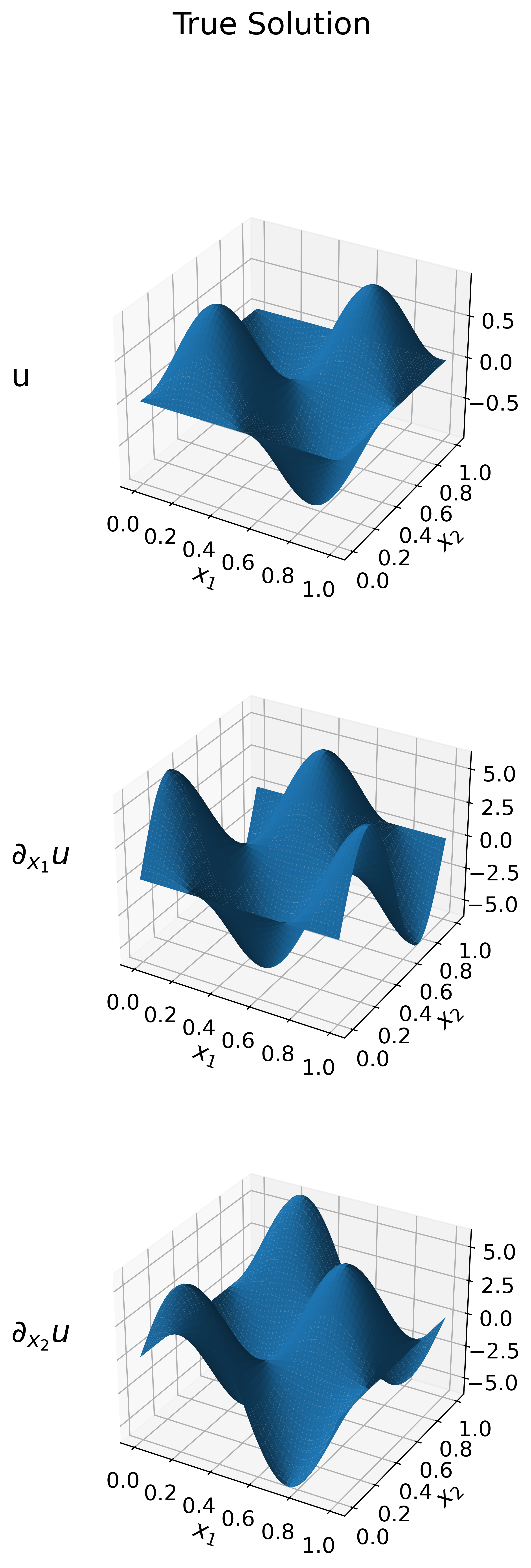
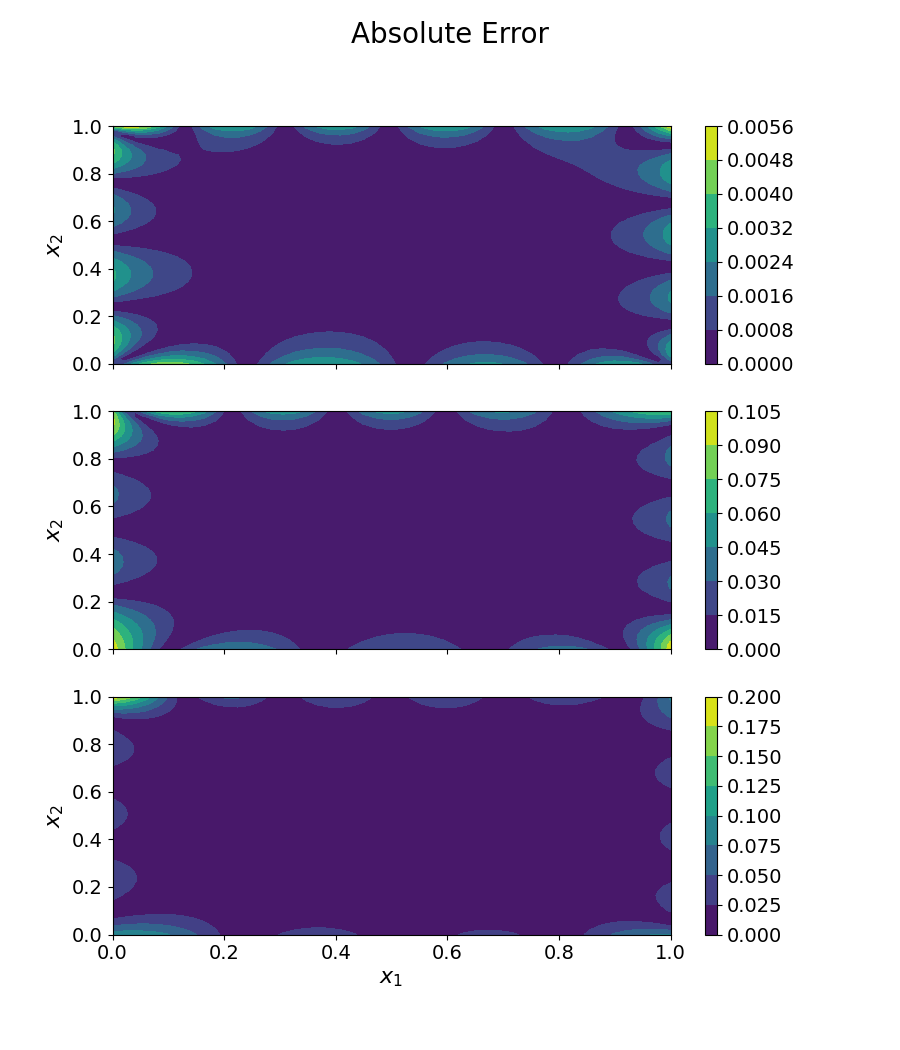
Figure 2. (Left) Comparison between the true solution from equation (6.1) (left) and the PINN approximation (middle) along with the absolute error (right).

6.2. Non-stationary case

We consider the Burgers equation with periodic boundary conditions on the domain $\Omega=[0,1]\times[0,1]$ with the forcing term

$$f(x_{1},x_{2},t)=-2\pi\exp(-4\pi^{2}\nu t) \left[(\cos(2\pi(x_{1}-t))+\cos(2\pi(x_{2}-t)))\right.$$

$$\left.(1-\exp(-4\pi^{2}\nu t)(\sin(2\pi(x_{1}-t))+\sin(2\pi(x_{2}-t))))\right]$$

and initial condition $u(x_{1},x_{2},0)=\sin(2\pi(x_{1}))\,\sin(2\pi(x_{2}))$.

For this setup, equation (4.1) admits the exact solution

$$u(x_{1},x_{2},t)=\exp(-4\pi^{2}\nu t)\,\sin(2\pi(x_{1}-t))\,\sin(2\pi(x_{2}-t)),$$ (6.2)

which serves as a reference to validate our error estimates. In our experiments, we use $\nu=0.01$.

Figure 3 compares the true solution from equation (6.2) with the PINN approximation at three time stamps $t=0,\,0.5$ and $1$. The left panel illustrates the exact solution, while the right panel shows the corresponding PINN-generated approximation.

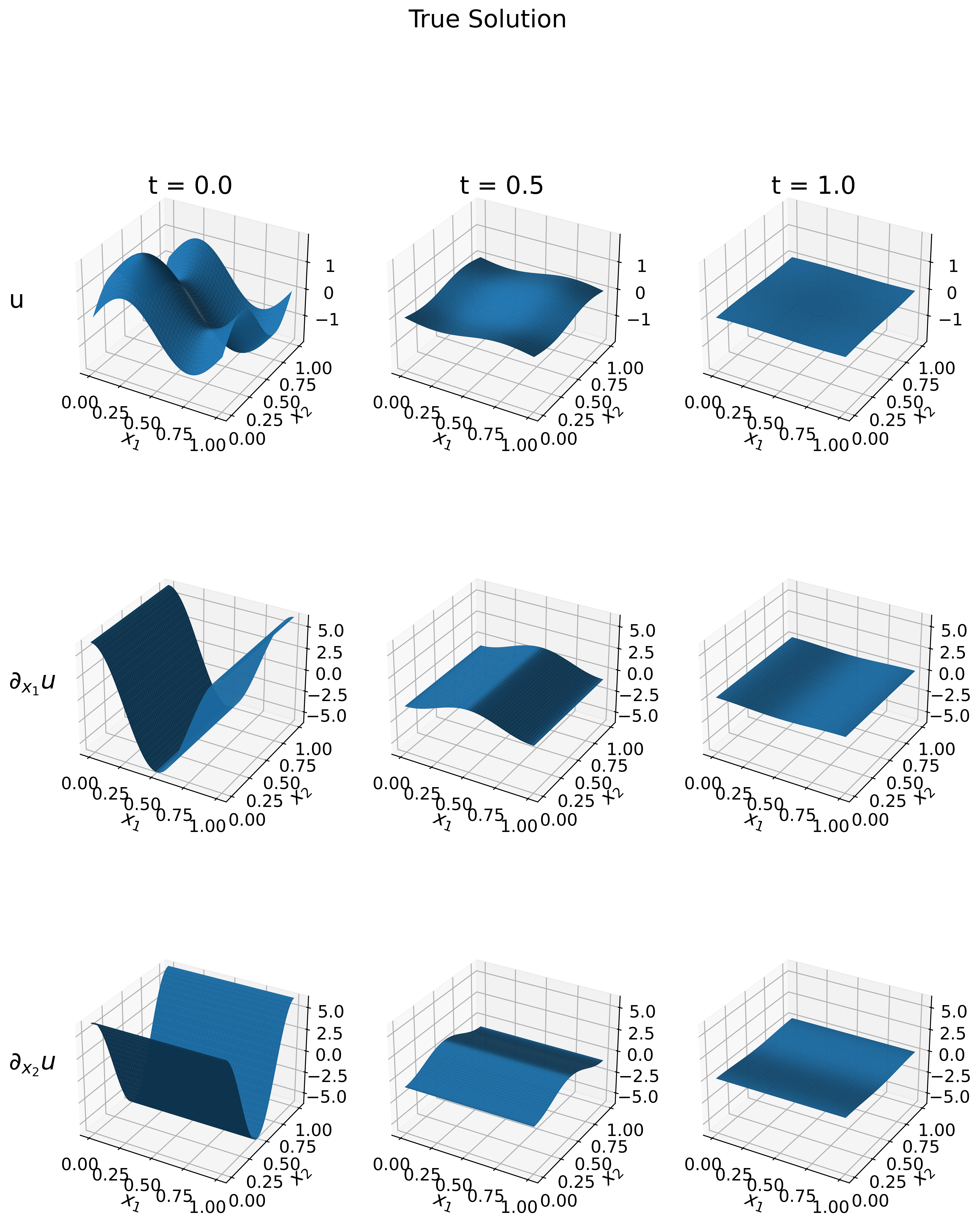
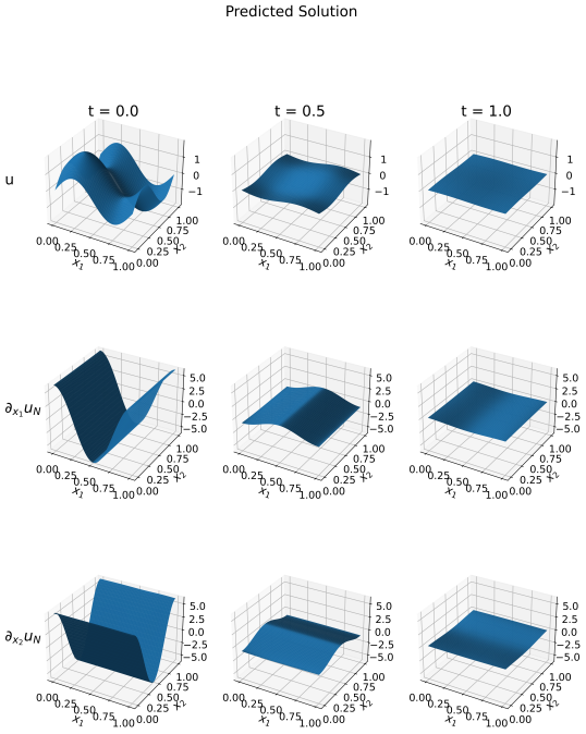
Figure 3. (Left) Comparison between the true solution from equation (6.2) (left) and the PINN approximation (right) at $t=0,0.5$ and $1$.

Figure 4 presents the absolute error between the true solution and the PINN approximation at $t=0,\,0.5$ and $1$. The error distribution highlights regions where the approximation deviates from the exact solution, providing insight into the model’s accuracy.

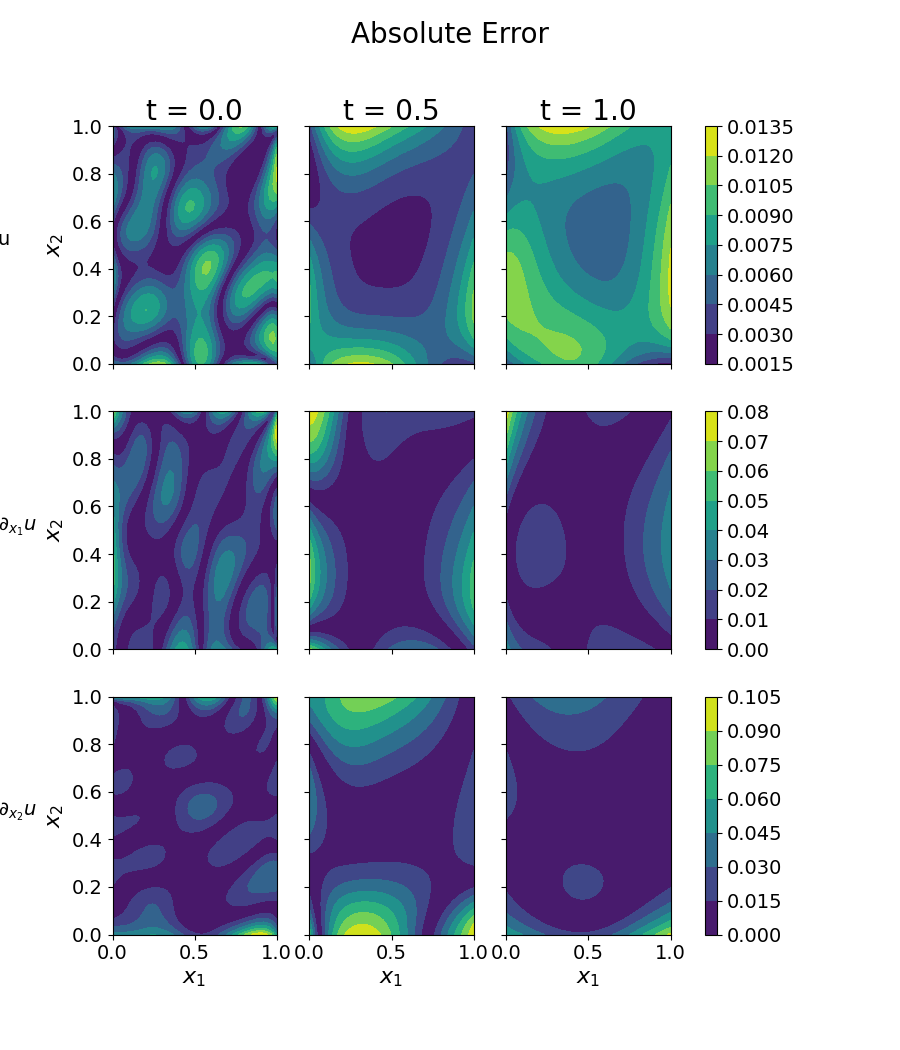
Figure 4. Absolute error between the true solution from equation (6.2) and the PINN approximation at $t=0,0.5$ and $1$.

Figure 5 depicts the $H^{1}$ error (dashed line) and the residual loss (solid line) as functions of time. While the exact value of the constant $C$ in Theorem 5.1 is unknown, the figure suggests that the two quantities are not significantly different, aligning with the behavior described in the theorem.

Time	H1 Error	Residual
$0$	$1.3\cdot 10^{-4}$	$2.47\cdot 10^{-3}$
$0.1$	$1.74\cdot 10^{-4}$	$2.73\cdot 10^{-3}$
$0.2$	$2.9\cdot 10^{-4}$	$2.27\cdot 10^{-3}$
$0.3$	$4.58\cdot 10^{-4}$	$1.95\cdot 10^{-3}$
$0.4$	$5.93\cdot 10^{-4}$	$1.8\cdot 10^{-3}$
$0.41$	$5.99\cdot 10^{-4}$	$1.79\cdot 10^{-3}$
$0.51$	$5.96\cdot 10^{-4}$	$1.59\cdot 10^{-3}$
$0.61$	$6.01\cdot 10^{-4}$	$1.6\cdot 10^{-3}$
$0.71$	$6.64\cdot 10^{-4}$	$1.59\cdot 10^{-3}$
$0.81$	$6.32\cdot 10^{-4}$	$1.69\cdot 10^{-3}$
$0.91$	$4.89\cdot 10^{-4}$	$1.71\cdot 10^{-3}$
$1$	$5.08\cdot 10^{-4}$	$2.23\cdot 10^{-3}$

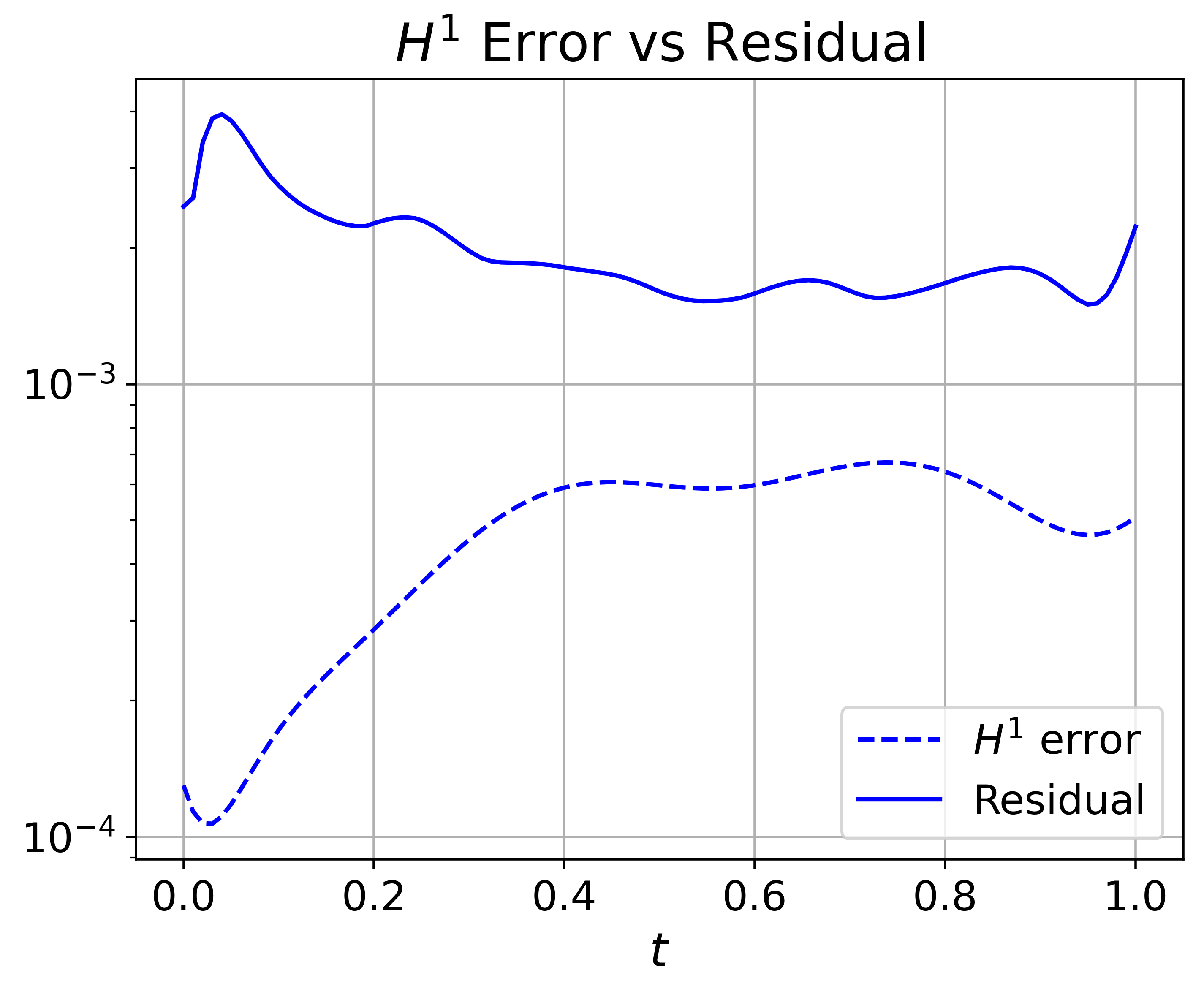
Figure 5. $H^{1}$ error between the true solution from equation (6.2) and the PINN approximation, along with the residual loss as a function of time, presented in a table (left) and as a figure (right).

References

• [1] S. Agmon, Lectures on elliptic boundary value problems, AMS Chelsea Publishing, Providence, RI, 2010, Prepared for publication by B. Frank Jones, Jr. with the assistance of George W. Batten, Jr., Revised edition of the 1965 original.
• [2] W. Akram, Feedback stabilization and finite element error analysis of viscous burgers equation around non-constant steady state, arXiv:2406.01553 (2024).
• [3] A. Bensoussan, G. D. Prato, M. C. Delfour, and S. K. Mitter, Representation and control of infinite dimensional systems, second ed., Systems & Control: Foundations & Applications, Birkhäuser Boston, Inc., Boston, MA, 2007.
• [4] A. Biswas, J. Tian, and S. Ulusoy, Error estimates for deep learning methods in fluid dynamics, Numer. Math. 151 (2022), no. 3, 753–777.
• [5] J. Caldwell, P. Wanless, and A. E. Cook, A finite element approach to Burgers’ equation, Appl. Math. Modelling 5 (1981), no. 3, 189–193.
• [6] J. R. Cannon, R. E. Ewing, Y. He, and Y. Lin, A modified nonlinear Galerkin method for the viscoelastic fluid motion equations, Internat. J. Engrg. Sci. 37 (1999), no. 13, 1643–1662.
• [7] Y. Chen and T. Zhang, A weak Galerkin finite element method for Burgers’ equation, J. Comput. Appl. Math. 348 (2019), 103–119.
• [8] A. Dogan, A Galerkin finite element approach to Burgers’ equation, Appl. Math. Comput. 157 (2004), no. 2, 331–346.
• [9] S. S. Dragomir, Some gronwall type inequalities and applications, Science Direct Working Paper No S1574-0358(04)70847-3, Available at SSRN: https://ssrn.com/abstract=3158353 187 (2003), 1–197.
• [10] L. C. Evans, Partial differential equations, second ed., Graduate Studies in Mathematics, vol. 19, American Mathematical Society, Providence, RI, 2010.
• [11] T. G. Grossmann, U. J. Komorowska, J. Latz, and C.-B. Schönlieb, Can physics-informed neural networks beat the finite element method?, IMA J. Appl. Math. 89 (2024), no. 1, 143–174.
• [12] C. F. Higham and D. J. Higham, Deep learning: an introduction for applied mathematicians, SIAM Rev. 61 (2019), no. 4, 860–891.
• [13] T. Kato, Strong $L^{p}$-solutions of the Navier-Stokes equation in ${\bf R}^{m}$, with applications to weak solutions, Math. Z. 187 (1984), no. 4, 471–480.
• [14] S. Kesavan, Topics in functional analysis and applications, John Wiley & Sons, Inc., New York, 1989.
• [15] A. Khan, M. T. Mohan, and R. Ruiz-Baier, Conforming, nonconforming and DG methods for the stationary generalized Burgers-Huxley equation, J. Sci. Comput. 88 (2021), no. 3, Paper No. 52, 26.
• [16] O. A. Ladyženskaja, V. A. Solonnikov, and N. N. Uralp̧rime ceva, Linear and quasilinear equations of parabolic type, Translations of Mathematical Monographs, vol. Vol. 23, American Mathematical Society, Providence, RI, 1968, Translated from the Russian by S. Smith.
• [17] J.-L. Lions and E. Magenes, Non-homogeneous boundary value problems and applications. Vol. I, II, Die Grundlehren der mathematischen Wissenschaften, vol. Band 182, Springer-Verlag, New York-Heidelberg, 1972.
• [18] Q. Lou, X. Meng, and G. E. Karniadakis, Physics-informed neural networks for solving forward and inverse flow problems via the boltzmann-bgk formulation, Journal of Computational Physics 447 (2021), 110676.
• [19] L. Lu, X. Meng, Z. Mao, and G. E. Karniadakis, DeepXDE: A deep learning library for solving differential equations, SIAM Review 63 (2021), no. 1, 208–228.
• [20] P. S. Mantri, N. Nataraj, and A. K. Pani, A qualocation method for Burgers’ equation, J. Comput. Appl. Math. 213 (2008), no. 1, 1–13.
• [21] W. McLean, Strongly elliptic systems and boundary integral equations, Cambridge University Press, Cambridge, 2000.
• [22] M. T. Mohan, $\mathbb{L}^{p}$-solutions of deterministic and stochastic convective Brinkman-Forchheimer equations, Anal. Math. Phys. 11 (2021), no. 4, Paper No. 164, 33.
• [23] M. T. Mohan and A. Khan, On the generalized Burgers-Huxley equation: existence, uniqueness, regularity, global attractors and numerical studies, Discrete Contin. Dyn. Syst. Ser. B 26 (2021), no. 7, 3943–3988.
• [24] L. Nirenberg, On elliptic partial differential equations, Ann. Scuola Norm. Sup. Pisa Cl. Sci. (3) 13 (1959), 115–162.
• [25] J. Novo and E. Terrés, Can neural networks learn finite elements?, J. Comput. Appl. Math. 453 (2025), Paper No. 116168, 8.
• [26] A. K. Pany, N. Nataraj, and S. Singh, A new mixed finite element method for Burgers’ equation, J. Appl. Math. Comput. 23 (2007), no. 1-2, 43–55.
• [27] M. Raissi, P. Perdikaris, and G. E. Karniadakis, Physics-informed neural networks: a deep learning framework for solving forward and inverse problems involving nonlinear partial differential equations, J. Comput. Phys. 378 (2019), 686–707.
• [28] M. Renardy and R. C. Rogers, An introduction to partial differential equations, Springer-Verlag, New York 13 (2004).
• [29] T. D. Ryck, A. D. Jagtap, and S. Mishra, Error estimates for physics-informed neural networks approximating the Navier-Stokes equations, IMA J. Numer. Anal. 44 (2024), no. 1, 83–119.
• [30] T. D. Ryck and S. Mishra, Error analysis for deep neural network approximations of parametric hyperbolic conservation laws, Math. Comp. 93 (2024), no. 350, 2643–2677.
• [31] by same author, Numerical analysis of physics-informed neural networks and related models in physics-informed machine learning, Acta Numer. 33 (2024), 633–713.
• [32] R. Temam, Navier-Stokes equations, AMS Chelsea Publishing, Providence, RI, 2001, Theory and numerical analysis, Reprint of the 1984 edition.
• [33] T. Xie and F. Cao, The errors of simultaneous approximation of multivariate functions by neural networks, Comput. Math. Appl. 61 (2011), no. 10, 3146–3152.