Towards a robust approach to infer causality in molecular systems satisfying detailed balance

Abstract

The ability to distinguish between correlation and causation of variables in molecular systems remains an interesting and open area of investigation. In this work, we probe causality in a molecular system using two independent computational methods that infer the causal direction through the language of information transfer. Specifically, we demonstrate that a molecular dynamics simulation involving a single Tryptophan in liquid water displays asymmetric information transfer between specific collective variables, such as solute and solvent coordinates. Analyzing a discrete Markov-state and Langevin dynamics on a 2D free energy surface, we show that the same kind of asymmetries can emerge even in extremely simple systems, undergoing equilibrium and time-reversible dynamics. We use these model systems to rationalize the unidirectional information transfer in the molecular system in terms of asymmetries in the underlying free energy landscape and/or relaxation dynamics of the relevant coordinates. Finally, we propose a computational experiment that allows one to decide if an asymmetric information transfer between two variables corresponds to a genuine causal link.

One of the most intriguing foundational questions in molecular science concerns how cause-and-effect relationships, plainly observed in our mesoscopic and macroscopic world, emerge from dynamic equations that are time-reversible at the microscopic scale. Measuring causality in a system described by classical equations of motion is highly non-trivial, and has been the object of intense investigation Gorecki et al. (2006); Kamberaj and van der Vaart (2009); Hacisuleyman and Erman (2017a, b); Sogunmez and Akten (2022); Hempel et al. (2020); Barr et al. (2011); Qi and Im (2013); Zhang et al. (2014); Sobieraj and Setny (2022); Zhu et al. (2022); Dutta et al. (2017); Perilla et al. (2013); Jo et al. (2015). For this purpose, molecular dynamics (MD) simulations offer the possibility to interrogate specific microscopic degrees of freedom that are often unattainable or very challenging to observe and manipulate in experimental approaches. In order to infer causality among Collective Variables (CVs) of interest, such as inter-residue distances Sobieraj and Setny (2022) or dihedral angles Dutta et al. (2017); Sogunmez and Akten (2022) in small proteins, various studies have previously analyzed MD simulations using Granger causality (GC) Granger (1969); Shojaie and Fox (2022), Transfer Entropy (TE) Schreiber (2000); Hlaváčková-Schindler et al. (2007) or time-lagged two-body cross-correlation functions (CCFs) Dutta et al. (2017); Hacisuleyman and Erman (2017a).

In other contexts, such as medical studies Wu et al. (2024), sociology Gangl (2010), and epidemiology Rothman and Greenland (2005), causal questions have been addressed for decades through the lens of causal inference Pearl (2009); Spirtes and Zhang (2016); Runge et al. (2023). This field provides a rigorous statistical framework to answer counterfactual questions such as “Had the value of variable $X$ been different, would the value of $Y$ have been different as well?”. The common strategy to address this question from observational time series, namely in the absence of ad-hoc manipulations of the putative causal variable $X$, is measuring conditional dependencies between pairs of variables at different times Runge (2018). Informally, if a variable $Y$ at time $\tau$ depends on a variable $X$ at time zero for all possible conditioning sets including the observed variables up to time $\tau$, one infers that $X$ causes $Y$. Crucially, this conclusion can be drawn only if no unobserved common cause of $X$ and $Y$ exists, or if all common causes of $X$ and $Y$ are included in the search space of conditioning sets. A common cause of two variables is typically referred to as “confounder”, and the hypothesis that all confounders are observed is referred to as “causal sufficiency”. While the most general algorithms to infer the causal graph rely on iterative conditional independence tests for each pair of variables Spirtes and Glymour (1991); Verma and Pearl (2022); Spirtes et al. (1993), an alternative approach in the case of time series is to compute the Transfer Entropy (TE), which is equivalent to carry out a single conditional independence test for each pair of variables Runge (2018). In the following, we will refer to any measure of conditional (in)dependence in observational time series data, such as TE, as information transfer.

If the existence of unobserved common drivers cannot be ruled out, one may assess the existence of a causal relationship $X\rightarrow Y$ by measuring the average or distributional changes in $Y$ resulting from two or more manipulations, or interventions, over $X$. A (hard) intervention on $X(0)$, denoted as $do(X(0)=x)$, is an ideal experiment where the value of $X$ at time zero is set to $x$ independently of the value of any other variable, observed or not, that is not caused by $X(0)$. Given two independent interventions $do\left(X(0)=x\right)$ and $do\left(X(0)=x^{\prime}\right)$, the causal effect of $X(0)$ on $Y(\tau)$ can be measured from the difference between the post-interventional distributions $p(Y(\tau)|do(X(0)=x))$ and $p(Y(\tau)|do(X(0)=x^{\prime}))$. Importantly, this interventional approach not only allows to formulate causal statements when unobserved common drivers are present, but also provides a direct quantification of causal effects Runge et al. (2019). Pearl’s “do-calculus” Pearl (2009) provides tools to compute post-interventional distributions from observational data, under the assumption of causal sufficiency.

In this work we investigate the emergence of strongly asymmetric information transfers, which indicate candidate unidirectional causal relationships, in molecular systems where the microscopic interactions are bidirectional due to Newton’s third law. In particular:

• Using an extremely simple molecular system, a Tryptophan (TRP) molecule solvated in water, we show that unidirectional information transfers between one-dimensional CVs can be inferred by measuring the Transfer Entropy Gorecki et al. (2006); Kamberaj and van der Vaart (2009); Hacisuleyman and Erman (2017a, b); Hempel et al. (2020); Barr et al. (2011); Perilla et al. (2013); Qi and Im (2013); Zhang et al. (2014); Jo et al. (2015); Sogunmez and Akten (2022), or using an approach introduced by some of us Tatto et al. (2024) when the CVs are high-dimensional (Sec. II).

• We show that such unidirectional information transfer can be present even in model systems which rigorously obey a time-reversible dynamics with stationary probability measure, such as a discrete-time Markov process, for which the Transfer Entropy can be computed analytically, and a Langevin dynamics on a two-dimensional potential energy surface (Sec. III).

• We show that if all the variables are observed, these asymmetries allow predicting the effect of suitable interventional experiments, for example a $do(X)$, in the language of causal inference. However, the presence of a unidirectional information transfer is not a sufficient condition to decide if a causal relationship exists: in a Langevin model with three variables in which only two are observed, we measure an asymmetric Transfer Entropy that does not correspond to a causal relationship. We show that this can be revealed by appropriate interventional experiments (Sec.  IV).

I Methods

We search for unidirectional information transfer between pairs of variables by estimating the Transfer Entropy and, for high-dimensional collective variables, by using the Imbalance Gain, an approach developed recently by some of us Tatto et al. (2024).

The Transfer Entropy, in its bivariate formulation, quantifies how the future state of a random variable $Y$ can be better predicted given the knowledge of the current states of both $Y$ and a second variable $X$, rather than using only the present state of $Y$ Schreiber (2000); Paluš et al. (2001). Given two time series $\{X_{t}\}_{t=0}^{T}$ and $\{Y_{t}\}_{t=0}^{T}$, we use the following definition of Transfer Entropy in direction $X\rightarrow Y$:

$$\text{TE}_{X\rightarrow Y}(\tau):=I(X_{0};Y_{\tau}\mid Y_{0})\,,$$ (1)

where $\tau$ is a discrete and positive time lag and $I(\cdot\,;\,\cdot\mid\cdot)$ is the conditional mutual information. Condition TE${}_{X\rightarrow Y}(\tau)>0$ is equivalent to the conditional dependence relationship $X_{0}\,\not\mathbf{\!\perp\!\!\!\perp}\,Y_{\tau}\mid Y_{0}$ (read: $Y_{\tau}$ depends on $X_{0}$ given $Y_{0}$), which allows stating the existence of a causal link (direct or indirect) from $X_{0}$ to $Y_{\tau}$, if $X$ and $Y$ are not affected by any common driver $Z$ (see Supp. Sec. S1). If the same measure in the opposite direction, TE_Y→X, is equal to zero after lag $\tau$, we say that the transfer of information from $X$ to $Y$ is (effectively) unidirectional after that time lag.

In molecular systems, the CVs describing the mesoscopic state are often intrinsically high-dimensional (for example, all the internal dihedrals of a protein molecule). Estimating Transfer Entropies between multidimensional variables requires estimating high-dimensional probability distributions, and is therefore computationally demanding. When necessary, we will quantify information transfer by the Imbalance Gain (IG) Tatto et al. (2024), a distance-based measure that we recently proposed to alleviate the practical limitations in computing Transfer Entropies between high-dimensional variables.

The Imbalance Gain probes conditional independence by a suitable rank statistics. Given a distance $d_{A}$, we define $r^{ij}_{A}$ the distance rank (or neighbour order) of $j$ with respect to $i$. Postulating that $d_{A}$ is informative with respect to a second distance $d_{B}$ when close points according to $d_{A}$ are also close according to $d_{B}$, the Information Imbalance Glielmo et al. (2022) from $d_{A}$ to $d_{B}$ is defined as

$$\Delta(d_{A}\rightarrow d_{B}):=\frac{2}{N}\langle r_{B}\mid r_{A}=1\rangle=\frac{2}{N^{2}}\sum_{i,j:\,r^{ij}_{A}=1}r^{ij}_{B}\,,$$ (2)

and it provides a number between 0 (maximum predictivity) and 1 (minimum predictivity). The former case occurs when all nearest neighbor pairs in $d_{A}$ remain nearest neighbor pairs in $d_{A}$, while the latter occurs when such pairs are randomly distributed in $d_{B}$. As shown in ref. Tatto et al. (2024), Eq. (2) can be extended to include $k$ nearest neighbors.

In the same spirit of Transfer Entropy and Granger Causality, in Ref. Tatto et al. (2024) we proposed to use Eq. 2 to verify whether the prediction of $d_{Y_{\tau}}$ can be improved by using a “mixed” distance space including both variables $X_{0}$ and $Y_{0}$, rather than $Y_{0}$ alone. Specifically, we translated the condition TE${}_{X\rightarrow Y}>0$ into the following inequality:

$$\Delta(\alpha):=\min_{\alpha}\Delta(d_{\alpha X_{0},\,Y_{0}}\rightarrow d_{Y_{\tau}})<\Delta(d_{Y_{0}}\rightarrow d_{Y_{\tau}})\,.$$ (3)

Equivalently, Eq. (3) can be written as $\delta\Delta_{X\rightarrow Y}>0$, by defining the Imbalance Gain (IG) in direction $X\rightarrow Y$ as Tatto et al. (2024)

$$\delta\Delta_{X\rightarrow Y}:=\frac{\Delta(\alpha=0)-\min_{\alpha}\Delta(\alpha)}{\Delta(\alpha=0)}\,.$$ (4)

We note that previous studies using data from equilibrium molecular dynamics simulations have also considered asymmetries in the time-lagged two-body cross correlation functions $\langle X_{0}Y_{\tau}\rangle$ to infer causal links Dutta et al. (2017); Hacisuleyman and Erman (2017a). However such correlation functions are invariant under the exchange of $X$ and $Y$: $\langle X_{0}Y_{\tau}\rangle=\langle X_{-\tau}Y_{0}\rangle=\langle X_{\tau}Y_{0}\rangle$ (the first equality holds under the assumption of stationarity, while the second follows from time-reversibility). Therefore, asymmetries in these correlation functions, if observed, can only be due to statistical errors, violations of time-reversibility induced by the integrator, and/or by the thermostat/barostat.

II Unidirectional information transfer between collective variables in a molecular system

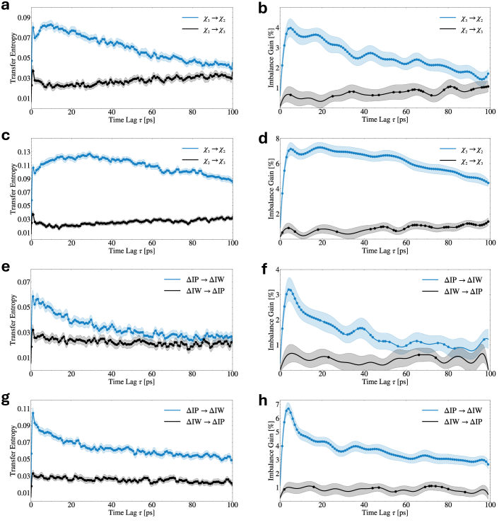
Figure 1: a and b: TE and IG curves for the CVs $\chi_{{}_{3}}$ and $\chi_{{}_{2}}$ in the GS. c and d: TE and IG curves for the same CVs in the ES. e and f: TE and IG curves for the CVs $\Delta\operatorname{IP}$ and $\Delta\operatorname{IW}$ in the GS. g and h: TE and IG curves for the same CVs in the ES. Shaded regions denote error bars over 14 independent estimates, and the bold points denote values that are determined to be significantly different from 0 using a t-test ($p<0.001$). The IG was computed using $k=5$ neighbors.

We first show that asymmetries in the Imbalance Gain and in the Transfer Entropy can be observed in a molecular system undergoing equilibrium and time-reversible dynamics. These asymmetries denote unidirectional information transfer between specific collective variables and, as we will see below, candidate causal links. Asymmetries in the TE have already been reported in several previous studies using molecular dynamics simulations (see for example Refs. Gorecki et al. (2006); Kamberaj and van der Vaart (2009); Hacisuleyman and Erman (2017a, b); Hempel et al. (2020); Barr et al. (2011); Perilla et al. (2013); Qi and Im (2013); Zhang et al. (2014); Jo et al. (2015); Sogunmez and Akten (2022)). TE is however limited to constructing probability distributions in low-dimensions, whereas the IG was introduced precisely to overcome this limitation.

We focus on molecular dynamics simulations of the amino-acid Tryptophan (TRP) in water. TRP is a naturally occurring fluorophore whose optical properties have been extensively studied to probe solvation dynamics - the response of protein and water coordinates following photoexcitation Nilsson and Halle (2005); Hassanali et al. (2006); Pal et al. (2002). We conducted microsecond-long equilibrium molecular dynamics (MD) simulations of TRP in water on both the ground and excited electronic states (GS and ES, respectively) in order to uncover unidirectional dependencies between specific solute and solvent coordinates. Our model of excitation mirrors previous studies that involve adjusting the point charges in the indole group to capture the change in the magnitude and direction of the dipole moment Hassanali et al. (2006); Li et al. (2007); Azizi et al. (2023) (see Supp. Sec. S2 for more details). From these simulations, we examined the relationships between a wide variety of variables that probe the coupling between the conformational changes of the TRP and the response of the surrounding water molecules. Figure S3 in Supp. Inf. shows a schematic of the structural coordinates that we examined. In addition to these structural quantities, we also examined variables that probe the changes in the interaction energy between the TRP and the environment arising from a photoexcitation. This can then be partitioned separately into contributions coming from the interactions of the chromophore (the indole moiety) with water molecules ($\operatorname{IW}$) and with the peptide chain ($\operatorname{IP}$).

In Fig. 1 we show pairs of collective variables displaying approximately unidirectional information transfer in the TE and IG, on the timescale of the first 100 ps. Figures 1a and 1b show the TE and IG between the $\chi_{{}_{3}}$ and $\chi_{{}_{2}}$ dihedral angles in the GS, respectively, while Figures 1c and 1d present the same measures in the ES. For both sets of simulations, we observe a large IG in direction $\chi_{{}_{3}}\rightarrow\chi_{{}_{2}}$, while the IG in the opposite direction is negligible. Similar behavior is also observed in the case of the TE. In the ES, the TE and IG from $\chi_{{}_{3}}$ to $\chi_{{}_{2}}$ decay on a much longer timescale compared to the GS; in addition, we observe that the unidirectional information transfer is more marked in the ES compared to the GS. The same behavior also holds for the CVs $\chi_{{}_{1}}$ and $\chi_{{}_{2}}$ (see Fig. S7 in the Supp. Inf.). This suggests that the timescales associated with the flow of information between different modes is altered in the GS versus ES.

In Figures 1 (panels e, f, g, h), we perform the same analysis for the energetic variables $\Delta\operatorname{IP}$ and $\Delta\operatorname{IW}$. These variables probe the total change in the electrostatic interaction energy between chromophore and peptide backbone (IP) or chromophore and water (IW), as a consequence of the excitation (see Supp. Sec. S3). In Figures 1e and 1f we show the TE and IG for the energetic variables in the GS, while in Figures 1g and 1h we report the same measures in the ES. In this case, we observe a unidirectional information transfer from $\Delta\operatorname{IP}$ to $\Delta\operatorname{IW}$. Similarly to the case of dihedrals, for the energetic variables the relaxation of both the TE and IG is significantly slowed down in the ES. It should be noted that for one-dimensional CVs the TE and the IG provide fully consistent results.

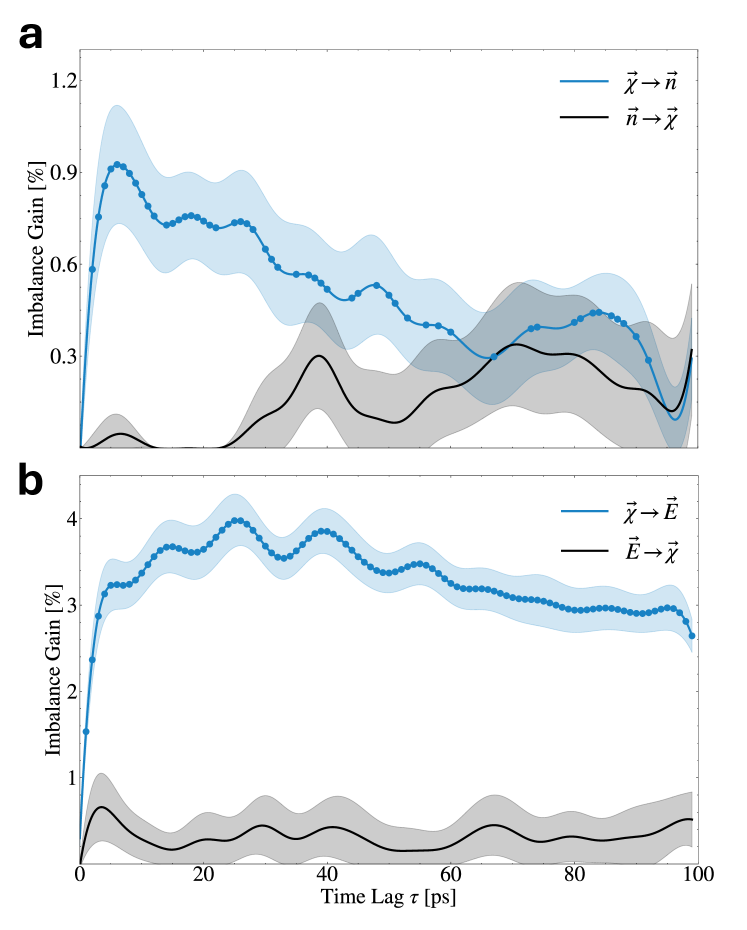
Figure 2: a: IG for $\vec{\chi}\rightarrow\vec{n}$ (blue) and $\vec{n}\rightarrow\vec{\chi}$ (black). b: IG for $\vec{\chi}\rightarrow\vec{E}$ (blue) and $\vec{E}\rightarrow\vec{\chi}$ (black). Shaded regions denote error bars over 14 independent estimates, and bold points denote values that are significantly different from 0 according to a t-test ($p<0.001$).

Next, we extend the analysis to multidimensional CVs, involving solvent coordinates and the energetic variables mentioned before. Conducting this type of analysis using TE is difficult due to the need to construct high-dimensional probability distributions. Fig. 2a shows the Imbalance Gain between two multidimensional CVs, $\vec{\chi}$ and $\vec{n}$, which represent a collection of dihedrals and coordination numbers, respectively. The dihedral vector, $\vec{\chi}=\left(\chi_{{}_{1}},\chi_{{}_{2}},\chi_{{}_{3}}\right)$, is composed of the 3 dihedrals discussed above and shown in Fig. S3, while $\vec{n}=\left(n_{\operatorname{CT}},n_{\operatorname{O1}},n_{\operatorname{O2}},n_{\operatorname{NT}},n_{\operatorname{NE1}}\right)$ includes the coordination numbers of the water oxygens with the C-terminus (CT), the carbonyl O atoms (O1 and O2), the N-terminus (NT), and the indole N-H (NE1). Fig. 2a shows the emergence of a unidirectional information transfer from $\vec{\chi}$ to $\vec{n}$. Finally, we computed the IG between $\vec{\chi}$ and $\vec{E}$, where $\vec{E}=\left(\Delta\operatorname{IP},\Delta\operatorname{IW}\right)$, which also unveils a clear asymmetry (Fig. 2b).

III Emergence of causal links in model systems at equilibrium

To interpret the results of the previous section we conducted a similar analysis on simple model systems: a discrete-time Markov process (Fig. 3a) and two Langevin dynamics on different free energy surfaces (FES) (Fig. 3d and g). In all these systems the dynamics satisfies detailed balance.

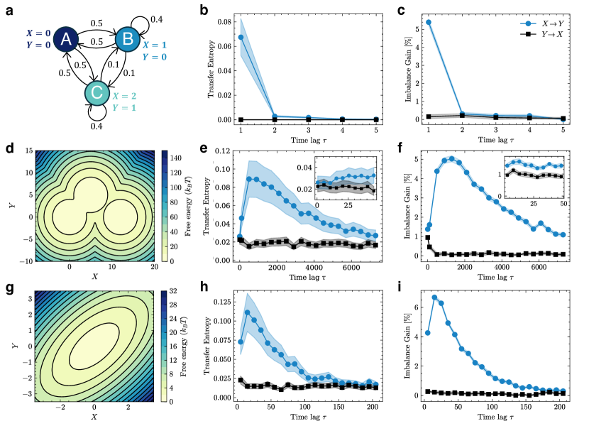
Figure 3: a: Markov diagram for a three-state system, with transition probabilities reported next to the arrows. $X$ and $Y$ are discrete dynamical variables whose values in each state are specified close to corresponding node. b and c: TE and IG from the dynamics generated by a, as a function of the time lag $\tau$. d: Asymmetric FES used for an overdamped Langevin dynamics with identical friction coefficients for $X$ and $Y$. e and f: TE and IG from the Langevin dynamics run over d. g: Symmetric FES used for an overdamped Langevin dynamics with different friction coefficients for $X$ and $Y$ ($\gamma_{X}=1$, $\gamma_{Y}=0.1$). h and i: TE and IG from the Langevin dynamics run over g. Shaded regions denote error bars over 20 independent estimates, each based on $N=2000$ trajectories. The IG was computed using $k=25$ neighbors.

In the Markov system of Fig. 3a, the three states A, B and C are uniquely identified by variable $X$, which assumes different values (0, 1 or 2) in each state. The second variable, $Y$, can only distinguish states A and B ($Y=0$) from state C ($Y=1$), but not A and B from each other. Therefore, $Y$ contains information that is redundant once the value of $X$ is known. For such a system, it is possible to show both analytically (Supp. Sec. S4) and numerically (Fig. 3b) that the TE is non-zero in direction $X\rightarrow Y$, while it is exactly zero in the reverse direction. This finding is reproduced by the IG as a function of the time lag $\tau$ (Fig. 3c), which is significantly different from zero only in direction $X\rightarrow Y$, and only for the time lag $\tau=1$. We note that in this system, the actual causal link from $X$ to $Y$ is instantaneous, as $Y_{t}$ is a deterministic function of $X_{t}$. Although TE and IG cannot directly test whether causal links are instantaneous, they can detect their presence at larger time lags (see Supp. Sec. S1).

As a second example, we consider an overdamped Langevin dynamics (see Supp. Sec. S5) carried out over the FES of Fig. 3d, which can be seen as a continuous version of the previous Markov system. Again, variable $X$ carries more information than $Y$ about the true state of the system, as the three minima can be distinguished by projecting the free energy along $X$, while only two minima can be identified by projecting along $Y$. This is sufficient to observe a TE unbalanced in direction $X\rightarrow Y$ (Fig. 3e and f), when time lags of order of the transition times are considered. The information transfer in direction $Y\rightarrow X$ is instead close to zero according to both measures. For smaller time lags, the thermal fluctuations within a single minimum play a role, and $Y$ still carries information about the state of the system that is not included in $X$. This is reflected by a non-zero information transfer from $Y$ to $X$ for very small $\tau$ (insets of Fig. 3e and f).

As a third example, we consider a Langevin dynamics in the FES of Fig. 3g, which is symmetric under the exchange of $X$ and $Y$. If the Langevin dynamics is generated using the same friction coefficient for both the variables, no information transfer asymmetry appears between $X$ and $Y$ (see Supp. Fig. S6). In contrast, using a smaller friction coefficient for $Y$ leads to the emergence of a clear unidirectional flow from $X$ to $Y$ (Figs. 3h and i).

Despite the differences, all previous examples describe a scenario where variable $X$ is already maximally predictive with respect to its own future, and variable $Y$ can only add redundant information on the future of $X$. In contrast, the uncertainty over the future of $Y$ can be reduced if the current state of $X$ is known.

Importantly, in the three examples such a “predictivity asymmetry” emerges from different mechanisms. In the first example, $X$ provides a complete description of the system’s state, while $Y$ describes the system with a certain level of degeneracy. While $X$ resolves the degeneracy of $Y$ by distinguishing states that are identical according to $Y$, the opposite is not true. In the second example, the system is two-dimensional, but the relaxation time within each minimum is much shorter than the transition times between the minima, so that the only information still retrievable at long time scales is the knowledge of the minimum in which the system is trapped. Therefore, $Y$ carries non-redundant information that allows improving the prediction of $X$ only for small time lags, but not in the far future, where all relevant information is already contained in $X$. In this case, $X$ and $Y$ are CVs retaining independent information of the true state, with $X$ being more informative than $Y$ in the long time-scale regime. In these first two examples, the asymmetric information transfer is rooted in the different information content that the variables retain about the true system’s state.

In the third example, the symmetry of the FES implies that $X$ and $Y$ retain the same level of information of the system’s state at a given time. However, such information levels become significantly different if referred to the future state of the system, as a consequence of the different relaxation times of $X$ and $Y$: while the description provided by $X$ at time zero can still be used as a good proxy of the system’s state at time $\tau$, the same does not apply for $Y$ if $Y$ has already equilibrated. In this scenario, the information transfer asymmetry is due to adiabatic separation: variable $X$ moves slowly, leaving to $Y$ the time to relax. In this condition, all the information on the long time-scale dynamics is provided by $X$ alone.

Figure 4: a and b: the FES for $\chi_{{}_{3}}$ and $\chi_{{}_{2}}$ in the GS and ES respectively. c and d: the FES for $\Delta\operatorname{IP}$ and $\Delta\operatorname{IW}$ in the GS and ES respectively.

The results described in Sec. II can be explained in light of the mechanisms just identified. In Figs. 4a and b we plot the FES as a function of the two dihedral angles ($\chi_{3}$ and $\chi_{2}$), for the GS and ES respectively. In the FES in Fig. 4a, more minima can be discerned by $\chi_{{}_{3}}$ than by $\chi_{{}_{2}}$. More precisely, the marginal free energies of the two angles (see Fig. S8 in Supp. Inf.) show three minima for $\chi_{{}_{3}}$ and two minima for $\chi_{{}_{2}}$, with a higher barrier for $\chi_{{}_{3}}$ ($\sim 6-9\,k_{B}T$) than for $\chi_{{}_{2}}$ ($\sim 4\,k_{B}T$). This indicates that $\chi_{{}_{3}}$ resolves the “degeneracies” of $\chi_{{}_{2}}$ more effectively than vice versa, or equivalently, that $\chi_{{}_{3}}$ serves as a better CV than $\chi_{{}_{2}}$. In the ES (Fig. 4b), some of the minima along $\chi_{{}_{3}}$ (specifically those in $(\chi_{{}_{2}},\chi_{{}_{3}})=(-2,1)$, $(\chi_{{}_{2}},\chi_{{}_{3}})=(1.5,-1.25)$ and $(\chi_{{}_{2}},\chi_{{}_{3}})=(-1.75,3)$) become more pronounced. As shown in Figures  1c and d, this leads to a more pronounced information transfer in direction $\chi_{{}_{3}}\rightarrow\chi_{{}_{2}}$. The slower decay of the TE and IG curves is determined by the deeper FES minima, which make $\chi_{{}_{3}}$ a slower mode in the ES than in the GS.

To further rationalize the asymmetries observed in Fig. 1, we turned to the FES between the two energetic variables, illustrated in Figures 4c and d. In sharp contrast to the FES involving the dihedrals, these distributions show a single broad minimum, which is only slightly asymmetric in the two variables. However, the two CVs display decorrelation times that are different for $\Delta\operatorname{IP}$ ($\sim$ 7 ps in the GS, $\sim$ 11 ps in the ES) and $\Delta\operatorname{IW}$ ($\sim$ 1 ps in the GS, $\sim$ 2 ps in the ES), making $\Delta\operatorname{IP}$ a slower CV than $\Delta\operatorname{IW}$ (see Supp. Fig. S9). This leads us to conclude that the asymmetric information transfer between the indole-peptide energetics and the indole-solvent energetics is a molecular example of the scenario shown earlier in Fig. 3 (panels g,h,e).

IV Asymmetries and the response to external interventions

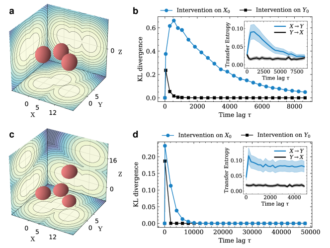
Figure 5: Effect of different interventions on two three-dimensional Langevin system with the same free energy projection in the $XY$-plane. a and c: Red spheres represent the free energy isosurface for $F=13\,k_{B}\,T$. The three planes show the free energy projections for all pairs variables. b and d: KL divergences between post-interventional distributions, intervening on $X_{0}$ (blue curves) and on $Y_{0}$ (black curves), as a function of the lag $\tau$ between the intervention and the time at which its effect is observed. Specifically, the two curves display $D_{KL}\left[p(Y_{\tau}\mid X_{0}=0)\|p(Y_{\tau}\mid X_{0}=12)\right]$ and $D_{KL}\left[p(X_{\tau}\mid Y_{0}=0)\|p(X_{\tau}\mid Y_{0}=5)\right]$, respectively.

In this section we will show that observing a unidirectional information transfer between two variables is a necessary, but not sufficient condition for the existence of a genuine causal link. Using the tools of causal inference, we analyze the behavior of the system in response to an active intervention, which we apply by setting a variable to a specific value, without changing any other variable that is not a direct cause of the manipulated one. In Langevin models, a “hard” intervention $do(X_{0}=x)$ can be thought to as an ideal experiment where the “natural” state of the system at time $t=0$, $(X_{0},Y_{0})$, is instantaneously set to $(x,Y_{0})$. After the external manipulation, the system is left free to evolve according to its unperturbed dynamics. Interventions provide an intuitive framework to speak about causality: we can state that $X$ causes $Y$ if and only if an intervention on $X_{0}$ leads to a measurable effect on $Y_{\tau}$ for some $\tau>0$. This effect can be quantified, for example, by measuring the Kullback-Leibler (KL) divergence between the distributions of $Y_{\tau}$ under two different interventions on $X_{0}$.

In Fig. 5 we show the effect of interventions on variables $X$ and $Y$ in two different three-dimensional model systems whose two-dimensional free energy as a function of $X$ and $Y$ is exactly identical to the free energy in Fig.  3d. We treat the third variable, $Z$, as if it were unobserved, computing only bivariate Transfer Entropies between $X$ and $Y$.

In the first system (top row) the $Z$ variable has the same distribution in the three minima, and the TE (inset in panel b) is qualitatively equivalent to the two-dimensional case shown in Fig. 3. In panel b we show the effect of $do(X_{0})$ and $do(Y_{0})$ experiments (blue and black curves, respectively), using as interventional values the positions of the furthest minima seen by each variable ($X_{0}=0,\,12$ and $Y_{0}=0,\,5$). The effect on $Y_{\tau}$ of the interventions on $X_{0}$ is still visible for large time lags, whereas the interventions on $Y_{0}$ have no effect on $X_{\tau}$ after a time scale comparable to the relaxation time within the minima. Therefore, in this example, the Transfer Entropy provides qualitatively the same information that one would infer by performing an external manipulation of the system.

In the second system (bottom row of Fig. 3), $Z$ does not distinguish the three minima seen by $X$, but reveals a fourth minimum, hidden for $X$, which features a higher free energy barrier than all “visible” barriers. The bivariate Transfer Entropy (inset of panel d) shows qualitatively the same asymmetry observed in the previous example, suggesting a unidirectional causal link $X\rightarrow Y$. However, intervening on $X_{0}$ affects $Y_{\tau}$ on significantly shorter time scales than those deducible from Transfer Entropy (blue curve in panel d). Thus, using Transfer Entropy to infer the existence of a causal effect of $X$ on $Y$ would lead to the wrong conclusion: over longer time-scales, the unobserved variable $Z$ behaves as a common driver of $X$ and $Y$. In Supp. Fig. S10 we support this statement by showing that an intervention on $Z_{0}$ results in a long-term effect on both $X_{\tau}$ and $Y_{\tau}$, while it has no effect when applied to the system of Fig. 5a.

V Discussion

In this work, we investigated the emergence of information transfer asymmetries in systems obeying equilibrium and time-reversible dynamics, and whether these asymmetries can be interpreted as causal links. We measured information transfers by using the Transfer Entropy and the Imbalance Gain. Crucially, both these observables efficaciously probe three-body dependencies, involving the present state of both the putative driver and the driven variables, and the future state of the latter. Standard time-lagged two-body cross-correlation functions (CCFs), which have been used to infer causal links from MD simulations Dutta et al. (2017); Hacisuleyman and Erman (2017a), cannot report on the directional flow of information between variables in stationary and time-reversible systems, as they are symmetric by construction. We illustrate this property by computing the CCFs between some of the relevant collective variables for TRP (see Supp. Figures S11 and S12).

Consistent with previous studies Gorecki et al. (2006); Kamberaj and van der Vaart (2009); Hacisuleyman and Erman (2017a, b); Sogunmez and Akten (2022); Hempel et al. (2020); Barr et al. (2011); Qi and Im (2013); Zhang et al. (2014); Sobieraj and Setny (2022); Zhu et al. (2022); Dutta et al. (2017); Perilla et al. (2013); Jo et al. (2015), we observed empirically that information transfer asymmetries can emerge even in a simple but realistic molecular system, namely a solvated TRP molecule. The choice of this system is motivated by Fluorescence Stokes Shift experiments, where TRP can be electronically excited by absorbing UV photons and used to probe solvation dynamics Vincent et al. (2000); Peon et al. (2002); Xu et al. (2006, 2015). Using model systems, we identified two mechanisms that explain the emergence of such asymmetries: (i) the asymmetry in the information content of different CVs, namely the capacity of one CV to describe states and transitions hidden to the others, and (ii) the discrepancy in their relaxation times. In particular, we found that the most informative CVs and the slowest CVs act as “sources” of information towards other CVs. Remarkably, all the asymmetries observed in the TRP system can be explained according to either one mechanism or the other. We also note that the first mechanism implies the second, as a CV that identifies more free energy minima can only relax on longer time-scales than a CV for which some minima are hidden. These findings provide enhanced insight into earlier studies Sobieraj and Setny (2022); Perilla and Woolf (2012), indicating that molecular descriptors selected by Granger Causality Sobieraj and Setny (2022) or Transfer Entropy Perilla and Woolf (2012) can accurately characterize transition states. The asymmetry of information flow also opens up interesting perspectives on how to measure the chemical physics of coupling between protein and water degrees of freedom Fenimore et al. (2004); Frauenfelder et al. (2006); Zhang et al. (2007). For the case of TRP, we observe that there is unidirectional flow of information from protein coordinates such as the dihedrals to the solvent. It would be interesting to understand the extent to which this directionality changes for tryptophan embedded in different chemical environments in proteins.

Information transfer asymmetries inferred on equilibrium dynamics are typically associated to causal relationships Kamberaj and van der Vaart (2009); Qi and Im (2013); Zhang et al. (2014); Jo et al. (2015). In this work, we have explicitly shown that such asymmetries are only a sufficient condition for inferring causal links, as unobserved CVs - namely, those not considered in the analysis - may act as common drivers of observed CVs. Specifically, if $Z$ identifies a higher free energy barrier than those observed by $X$ and $Y$, $Z$ behaves as a common driver of $X$ and $Y$ on time scales comparable with the transition time to the hidden minimum.

Our findings suggest two possible routes for discovering causal relationships in molecular systems: either using a set of CVs that can be safely assumed to be “causally sufficient" – that is, unaffected by unobserved common drivers, or performing explicit interventional experiments on CVs of interest. The first approach is viable by considering a large pool of CVs, such as all key dihedrals of a molecule Sobieraj and Setny (2022), and estimating information transfers in a multivariate fashion (see Supp. Sec. S1). This approach is unavoidably affected by the curse of dimensionality as the number of CVs increases, although methodologies designed for high-dimensional settings, such as the IG and its extensions Allione et al. (2025), promise to alleviate this issue.

The second approach necessitates the design of interventional experiments on molecular CVs. This approach sounds natural in a simulation setting, in which one can perform arbitrary manipulations on the system, but poses some practical challenges. In particular, the interventional experiments that we carried out on the model systems (Sec. IV) were applied to “orthogonal” CVs $X$ and $Y$, such that an instantaneous variation of $X$ at time $t=0$ does not affect $Y$ at the same time. This may be the case for CVs that describe spatially separated regions of a molecular system, such as distant sites within a protein. However, CVs of interest can also depend on a common subset of degrees of freedom that generate instantaneous dependencies. In this scenario, setting $X(0)$ to an arbitrary value ($do(X(0)=x)$) may be practically impossible without changing also $Y(0)$. As an example, in our TRP system, the dihedrals $\chi_{{}_{1}},\chi_{{}_{2}}$ and $\chi_{{}_{3}}$ depend on common atomic positions affected by rigid constraints, and in turn, not all arbitrary choices of such angles are possible. Moreover, “hard” interventions such as those applied in this work appear challenging in molecular dynamics simulations, as they would require an instantaneous modification of several degrees of freedom, making it necessary to develop appropriate protocols. The design of suitable interventional experiments on molecular CVs will be the subject of future work.

Data Availability Statement

The data that support the findings of this study are available from the corresponding author upon reasonable request.

References

- Gorecki et al. (2006) A. Gorecki, J. Trylska, and B. Lesyng, Europhysics Letters 75, 503 (2006).
- Kamberaj and van der Vaart (2009) H. Kamberaj and A. van der Vaart, Biophysical Journal 97, 1747 (2009).
- Hacisuleyman and Erman (2017a) A. Hacisuleyman and B. Erman, PLOS Computational Biology 13, 1 (2017a).
- Hacisuleyman and Erman (2017b) A. Hacisuleyman and B. Erman, Proteins: Structure, Function, and Bioinformatics 85, 1056 (2017b), https://onlinelibrary.wiley.com/doi/pdf/10.1002/prot.25272 .
- Sogunmez and Akten (2022) N. Sogunmez and E. D. Akten, Applied Sciences 12, 8530 (2022).
- Hempel et al. (2020) T. Hempel, N. Plattner, and F. Noé, Journal of Chemical Theory and Computation 16, 2584 (2020), https://doi.org/10.1021/acs.jctc.0c00043 .
- Barr et al. (2011) D. Barr, T. Oashi, K. Burkhard, S. Lucius, R. Samadani, J. Zhang, P. Shapiro, A. D. J. MacKerell, and A. van der Vaart, Biochemistry 50, 8038 (2011), https://doi.org/10.1021/bi200503a .
- Qi and Im (2013) Y. Qi and W. Im, Journal of Chemical Theory and Computation 9, 3799 (2013), https://doi.org/10.1021/ct4002784 .
- Zhang et al. (2014) L. Zhang, T. Centa, and M. Buck, The Journal of Physical Chemistry B 118, 7302 (2014), https://doi.org/10.1021/jp503668k .
- Sobieraj and Setny (2022) M. Sobieraj and P. Setny, Journal of Chemical Theory and Computation 18, 1936 (2022), https://doi.org/10.1021/acs.jctc.1c00945 .
- Zhu et al. (2022) J. Zhu, J. Wang, W. Han, and D. Xu, Nature Communications 13, 1 (2022).
- Dutta et al. (2017) S. Dutta, M. Ghosh, and J. Chakrabarti, Scientific Reports 7, 40439 (2017).
- Perilla et al. (2013) J. R. Perilla, D. J. Leahy, and T. B. Woolf, Proteins: Structure, Function, and Bioinformatics 81, 1113 (2013), https://onlinelibrary.wiley.com/doi/pdf/10.1002/prot.24257 .
- Jo et al. (2015) S. Jo, Y. Qi, and W. Im, Glycobiology 26, 19 (2015), https://academic.oup.com/glycob/article-pdf/26/1/19/17485946/cwv083.pdf .
- Granger (1969) C. W. J. Granger, Econometrica 37, 424–438 (1969).
- Shojaie and Fox (2022) A. Shojaie and E. B. Fox, Annual Review of Statistics and Its Application 9, 289 (2022).
- Schreiber (2000) T. Schreiber, Phys. Rev. Lett. 85, 461 (2000).
- Hlaváčková-Schindler et al. (2007) K. Hlaváčková-Schindler, M. Paluš, M. Vejmelka, and J. Bhattacharya, Physics Reports 441, 1 (2007).
- Wu et al. (2024) X. Wu, S. Peng, J. Li, J. Zhang, Q. Sun, W. Li, Q. Qian, Y. Liu, and Y. Guo, Applied Intelligence 54, 1 (2024).
- Gangl (2010) M. Gangl, Annual Review of Sociology 36, 21 (2010).
- Rothman and Greenland (2005) K. J. Rothman and S. Greenland, American Journal of Public Health 95, S144 (2005), https://doi.org/10.2105/AJPH.2004.059204 .
- Pearl (2009) J. Pearl, Causality: Models, Reasoning and Inference, 2nd ed. (Cambridge University Press, USA, 2009).
- Spirtes and Zhang (2016) P. Spirtes and K. Zhang, Appl. Inform. 3, 1–28 (2016).
- Runge et al. (2023) J. Runge, A. Gerhardus, G. Varando, V. Eyring, and G. Camps-Valls, Nature Reviews Earth & Environment 4 (2023), 10.1038/s43017-023-00431-y.
- Runge (2018) J. Runge, Chaos: An Interdisciplinary Journal of Nonlinear Science 28, 075310 (2018).
- Spirtes and Glymour (1991) P. Spirtes and C. Glymour, Social Science Computer Review 9, 62 (1991), https://doi.org/10.1177/089443939100900106 .
- Verma and Pearl (2022) T. Verma and J. Pearl, “Equivalence and synthesis of causal models,” in Probabilistic and Causal Inference: The Works of Judea Pearl (Association for Computing Machinery, New York, NY, USA, 2022) p. 221–236, 1st ed.
- Spirtes et al. (1993) P. Spirtes, C. Glymour, S. N., and Richard, Causation, Prediction, and Search (Mit Press: Cambridge, 1993).
- Runge et al. (2019) J. Runge, P. Nowack, M. Kretschmer, S. Flaxman, and D. Sejdinovic, Science Advances 5, eaau4996 (2019), https://www.science.org/doi/pdf/10.1126/sciadv.aau4996 .
- Tatto et al. (2024) V. D. Tatto, G. Fortunato, D. Bueti, and A. Laio, Proceedings of the National Academy of Sciences 121, e2317256121 (2024), https://www.pnas.org/doi/pdf/10.1073/pnas.2317256121 .
- Paluš et al. (2001) M. Paluš, V. Komárek, Z. c. Hrn číř, and K. Štěrbová, Phys. Rev. E 63, 046211 (2001).
- Glielmo et al. (2022) A. Glielmo, C. Zeni, B. Cheng, G. Csányi, and A. Laio, PNAS Nexus 1, pgac039 (2022), https://academic.oup.com/pnasnexus/article-pdf/1/2/pgac039/58561052/pgac039.pdf .
- Nilsson and Halle (2005) L. Nilsson and B. Halle, Proceedings of the National Academy of Sciences 102, 13867–13872 (2005).
- Hassanali et al. (2006) A. A. Hassanali, T. Li, D. Zhong, and S. J. Singer, The Journal of Physical Chemistry B 110, 10497–10508 (2006).
- Pal et al. (2002) S. K. Pal, J. Peon, B. Bagchi, and A. H. Zewail, The Journal of Physical Chemistry B 106, 12376 (2002), https://doi.org/10.1021/jp0213506 .
- Li et al. (2007) T. Li, A. A. Hassanali, Y.-T. Kao, D. Zhong, and S. J. Singer, Journal of the American Chemical Society 129, 3376 (2007).
- Azizi et al. (2023) K. Azizi, M. Gori, U. Morzan, A. Hassanali, and P. Kurian, PNAS Nexus 2, pgad257 (2023).
- Vincent et al. (2000) M. Vincent, A.-M. Gilles, I. M. Li De La Sierra, P. Briozzo, O. Bârzu, and J. Gallay, The Journal of Physical Chemistry B 104, 11286–11295 (2000).
- Peon et al. (2002) J. Peon, S. K. Pal, and A. H. Zewail, Proceedings of the National Academy of Sciences 99, 10964–10969 (2002).
- Xu et al. (2006) J. Xu, D. Toptygin, K. J. Graver, R. A. Albertini, R. S. Savtchenko, N. D. Meadow, S. Roseman, P. R. Callis, L. Brand, and J. R. Knutson, Journal of the American Chemical Society 128, 1214–1221 (2006).
- Xu et al. (2015) J. Xu, B. Chen, P. Callis, P. L. Muiño, H. Rozeboom, J. Broos, D. Toptygin, L. Brand, and J. R. Knutson, The Journal of Physical Chemistry B 119, 4230–4239 (2015).
- Perilla and Woolf (2012) J. R. Perilla and T. B. Woolf, The Journal of Chemical Physics 136, 164101 (2012), https://pubs.aip.org/aip/jcp/article-pdf/doi/10.1063/1.3702447/14731500/164101_1_online.pdf .
- Fenimore et al. (2004) P. W. Fenimore, H. Frauenfelder, B. H. McMahon, and R. D. Young, Proceedings of the National Academy of Sciences 101, 14408 (2004).
- Frauenfelder et al. (2006) H. Frauenfelder, P. W. Fenimore, G. Chen, and B. H. McMahon, Proceedings of the National Academy of Sciences 103, 15469–15472 (2006).
- Zhang et al. (2007) L. Zhang, L. Wang, Y.-T. Kao, W. Qiu, Y. Yang, O. Okobiah, and D. Zhong, Proceedings of the National Academy of Sciences 104, 18461–18466 (2007).
- Allione et al. (2025) M. Allione, V. D. Tatto, and A. Laio, “Linear scaling causal discovery from high-dimensional time series by dynamical community detection,” (2025), arXiv:2501.10886 [physics.data-an] .