A Nonlinear Extension of the Variable Projection (VarPro) Method for NURBS-based Conformal Surface Flattening

Abstract

In the field of computer graphics, conformal surface flattening methods have been extensively studied because they are useful in applications such as texture mapping, geometry processing, and mesh generation. However, most approaches aim to flatten a given input geometry while preserving the conformal property as much as possible. In other words, the resulting flattening is only as conformal as possible to the target surface. By contrast, this study focuses on a special class of surfaces that admits accurate conformal flattening. In this scenario, conformal flattening becomes a coupled problem: the input (or target) surface must be recursively refined while its flattening is being determined. Indeed, the uniformization theorem or the Riemann mapping theorem guarantees the existence of a conformal flattening for any surface, provided that the surface is simply connected and orientable. However, these theorems allow the conformal flattening to include singularities. If singularities are not permitted, then only a special class of surfaces admits conformal flattening—although many surfaces do fall within this class.

In this paper, we develop a nonuniform rational B-splines (NURBS)-based approach in which both the input surface and its flattening are simultaneously refined, thereby ensuring they remain mutually conformal. Because NURBS surfaces cannot represent singularities, a pair of mutually conformal surfaces taht do not have singularities are naturally obtained. Our approach is inspired by the form-finding method presented in [9, 10], which allows bilinear partial differential equations (PDEs) to be solved by iteratively refining two surfaces in concert. Building on their demonstration that the variable projection (VarPro) method is highly effective, we also attempt to employ VarPro. VarPro is a computational scheme that alternately executes a linear projection and a nonlinear iteration by assuming the problem is partially linear (separable). Because our conformal condition is separable into two nonlinear subproblems, we propose a nonlinear extension of VarPro. Although this generalization significantly increases the computational cost, the quality of the results is noteworthy.

Keywords: Conformal mapping, conformal flattening, variable projection (VarPro) method, nonlinear least squares problems

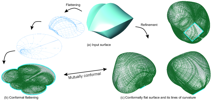
Figure 1: We present a novel conformal surface flattening algorithm that targets nonunifrom rational B-splines (NURBS) surfaces. This method is a nonlinear extension of the variable projection (VarPro) method. While most existing conformal flattening algorithms find as-conformal-as possible flattening by regarding the input surface as given, our method attempts to simultaneously refine both the target and the flattened surfaces so that the generated surfaces are mutually conformal. (a) An input surface. (b) A flattened surface. (c) A ”refined” surface that is conformal to (b).

1 Introduction

Conformal surface flattening (or conformal surface parametrization) has been actively studied in geometry and computer graphics because it is useful for applications such as texture mapping, geometry processing, and mesh generation. Two surfaces are mutually conformal when the angle between any pair of tangent vectors at each point is preserved under the projection. In such mappings, the local stretch is uniform in every direction around each point. For instance, a tiny illustration of an elephant drawn on one surface will appear to be the same elephant on the other surface, albeit scaled. Thus, conformal mapping locally preserves shapes, which is the reason for its wide range of applications.

To date, numerous mesh-based conformal flattening methods have been proposed, such as least-squares conformal maps [8], angle-based flattening [14], and spectral conformal parametrization methods [3, 4]. Additional methods can be found in [6, 15, 13]. However, because these methods take the input surface as given, they are limited to producing the best possible conformal flattening for that fixed surface.

In this study, we are interested in a special class of surfaces that have accurate conformal flattening. In this case, conformal flattening is fundamentally a coupled problem; the target surface must also be refined during the flattening process. Indeed, the uniformization theorem or the Riemann mapping theorem guarantees the existence of a conformal flattening for any surface, provided that the surface is simply connected and orientable. However, these theorems allow the conformal flattening to include singularities. If singularities are not permitted, then only a special class of surfaces admits conformal flattening—although many surfaces do fall within this class.

In this paper, we present a novel NURBS-based approach in which one simultaneously computes a pair of mutually conformal surfaces—a curved target surface and its corresponding planar flattening. Our algorithm concurrently refines both surfaces, as depicted in Fig. 1, thereby ensuring that they remain mutually conformal.

Our approach is simply to collect all the least-squares errors of all the conditions to form a nonlinear least-squares minimization problem and solve it. Because our problem is one in which variables are naturally grouped into two groups, we explore several approaches developed for this type of problem, including the Gauss–Newton method and the variable projection (VarPro) method. Finally, we propose an inner–outer iterative algorithm as a nonlinear extension of VarPro that can effectively solve nonlinear problems that are separable into two mildly nonlinear subproblems. Thus, finding a mildly linear form for each condition is the key in this work.

2 Methodological Formulation

In this section, we begin by summarizing the basic concepts of differential geometry and then introduce the conditions we solve in our method.

2.1 The first and second fundamental forms

Let us denote the position vector of a parametric surface as

$$\boldsymbol{R}(\theta^{1},\theta^{2})=\left[x(\theta^{1},\theta^{2})\>y(\theta^{1},\theta^{2})\;z(\theta^{1},\theta^{2})\right]^{T},$$ (1)

where $\theta^{1}$ and $\theta^{2}$ are coordinate parameters, and $x,y,z$ are the Cartesian coordinates of the point on the surface at $(\theta^{1},\theta^{2})$.

On this coordinate system, the basis vectors are defined as

$$\boldsymbol{g}_{i}=\partial_{i}\boldsymbol{R}.$$ (2)

Using this, the first fundamental form, or the metric tensor, is defined as

$$g_{ij}=\boldsymbol{g}_{i}\cdot\boldsymbol{g}_{j}.$$ (3)

At each point of a surface, the lengths of tangent vectors and the angles between the tangent vectors can be measured using this matrix.

In classical differential geometry, we also define the second fundamental form as follows:

$$b_{ij}=\partial_{ij}\boldsymbol{R}\cdot\boldsymbol{N},$$ (4)

where $\boldsymbol{N}$ is a normalized normal vector computed as

$$\boldsymbol{N}=\frac{\boldsymbol{g}_{1}\times\boldsymbol{g}_{2}}{\sqrt{g}},g=\mathrm{det}g_{ij}.$$ (5)

Using the second fundamental form, we can measure the normal curvature along certain directions.

2.2 Method: input and goal

Our goal is to obtain a pair of G2-continuous watertight NURBS surfaces that are mutually conformal, with one curved (i.e., a target surface) and the other flat (i.e., a flattening). Our algorithm takes a collection of watertight NURBS surfaces as input. This surface does not need to be G1- or G2-continuous; it can have creases along shared edges between adjacent patches. The G1- and G2-continuity conditions are eventually ensured via our nonlinear least-squares minimization algorithm.

In the initial step, this algorithm duplicates the input surface into two surfaces: One is used as the initial surface for the target surface, and the other is used as the initial surface for the flattening. Then, two surfaces are recursively updated via our algorithm (see Section 3). During the flattening process, several conditions are enforced on two surfaces, which are described below. In addition to the input surface, the user must provide a flat surface as a reference surface, which is different from the conformal flattening and is used to ensure the G1- and G2- continuity conditions of the target surface and the flattening. The reference surface is not updated during the computation.

Because we literally flatten surfaces, the surface must have at least one hole, or a boundary loop. For simplicity, we only discuss the fixed-edge condition for the target surface.

2.3 Flat condition

To flatten the flattening, we initially thought that enforcing

$$N_{x}=0,\;N_{y}=0,N_{z}=1$$ (6)

all over the surface domain was enough. However, this condition is highly nonlinear and makes the proposed method unreliable. This is understandable, as a normalized vector generally rotates on a sphere.

Thus, we used the following mildly nonlinear forms instead:

$$\begin{split}D_{x}=\frac{\partial_{1}\eta\partial_{2}\phi-\partial_{1}\phi\partial_{2}\eta}{\sqrt{\bar{g}}}&=0,\\ D_{y}=\frac{\partial_{1}\phi\partial_{2}\xi-\partial_{1}\xi\partial_{2}\phi}{\sqrt{\bar{g}}}&=0,\\ D_{z}=\frac{\partial_{1}\xi\partial_{2}\eta-\partial_{1}\eta\partial_{2}\xi}{\sqrt{\bar{g}}}&=\frac{\sqrt{e}}{\sqrt{\bar{g}}},\\ \end{split}$$ (7)

, where three functions represent the $x,y$ and $z$ coordinates of each point of the flattening. Note that, although $e$ is guaranteed to be positive, it can be negative in areas where two directions are almost parallel due to numerical round-off errors. If that’s the case, $\sqrt{e}$ turns NaN. Hence, careful exception handling is needed here.

2.4 Conformal condition

We denote the metric tensors of the target surface and the flattening as $g_{ij}$ and $e_{ij}$, respectively. Then, the conformal property is written as

$$e_{ij}=\lambda g_{ij},$$ (8)

where $\lambda$ is the scaling factor proven to be a harmonic function. As this harmonic property is naturally satisfied when a conformal flattening is obtained, it is enough to regard $\lambda$ as an arbitrary real number. Hence, this condition is equivalent to the following three conditions:

$$\begin{split}g_{11}e_{12}&=g_{12}e_{11}\\ g_{12}e_{22}&=g_{22}e_{12}\\ g_{22}e_{11}&=g_{11}e_{22}\\ .\end{split}$$ (9)

As is obvious, only two out of the three conditions are independent, and we can select any two of them. In our implementation, we selected the first two conditions.

Because it is desired to make the condition unit-less, we instead solve

$$\frac{g_{11}}{\sqrt{\bar{g}}}\frac{e_{12}}{\sqrt{\bar{g}}}=\frac{g_{12}}{\sqrt{\bar{g}}}\frac{e_{11}}{\sqrt{\bar{g}}},\;\frac{g_{12}}{\sqrt{\bar{g}}}\frac{e_{22}}{\sqrt{\bar{g}}}=\frac{g_{22}}{\sqrt{\bar{g}}}\frac{e_{12}}{\sqrt{\bar{g}}}$$ (10)

where $\bar{g}$ is the determinant of the first fundamental form in the reference surface. We do not use the updated values of the determinants of $g_{ij}$ or $e_{ij}$ in order to keep the condition only mildly nonlinear. As far as we tested, dividing them by $\sqrt{g}$ and $\sqrt{e}$ immediately makes the method unreliable. For further details, please refer to the discussion about nonlinearity in section 6. This is the primary condition we tackle in the current study.

These are bi-nonlinear PDEs that we tackle in this study. Because the condition is highly nonlinear and the problem is described with two conditions against two unknown functions, the solution space can easily vanish when the target surface is fixed. In contrast, if we regard the target surface as unknown, the problem is described with five unknown functions, and thus, many solutions are to be expected.

2.5 Point handles

To control the target surface so that we can obtain a desired shape, we need a few point handles that constrain several points on the target surface to specific positions—typically the initial positions on the input surface. This condition is given by

$$x=\bar{x},\;y=\bar{y}\;z=\bar{z}$$ (11)

where barred symbols represent the target coordinates.

2.6 Continuity conditions and reference surface

The G1-continuous condition of a surface requires the tangent planes of adjacent NURBS patches to overlay. This determines one condition. However, as we deal with three independent functions, there should be three independent G1-continuity conditions in principle, and thus, we aim to make three functions independently G1-continuous.

For that sake, we set up a reference surface, a flat surface with the same topology as the target surface and the flattening. The basic idea is that we assume $x,y$ and $z$ are all G-1 continuous on the reference surface and allow only deformations that preserve the G-1 continuity.

On the reference surface, we define the basis vectors, the first fundamental form, etc. as

$$\bar{\boldsymbol{g}}_{i}=\partial_{i}\boldsymbol{\bar{r}},\;\bar{g}_{ij}=\boldsymbol{\bar{g}}_{i}\cdot\bar{\boldsymbol{g}}_{j},\;\{\bar{g}^{ij}\}=\{\bar{g}_{ij}\}^{-1},\;\boldsymbol{\bar{g}}^{i}=\bar{g}^{ij}\boldsymbol{\bar{g}}_{j},$$ (12)

where $\bar{\boldsymbol{r}}$ is the position vector of the reference surface and $\bar{\boldsymbol{g}}^{i}$ are dual basis vectors.

To determine continuity conditions at any point on an edge curve shared by two adjacent NURBS patches, we define a tangent vector perpendicular to the edge:

$$\bar{w}^{i}=\bar{\epsilon}^{im}\bar{g}_{mn}\bar{v}^{n},$$ (13)

where $\bar{v}^{i}$ is a normalized vector parallel to the edge and $\bar{\epsilon}^{im}$ is the alternator determined on the reference surface. The alternator is defined as

$$\bar{\epsilon}^{11}=\bar{\epsilon}^{22}=0,\bar{\epsilon}^{12}=-\bar{\epsilon}^{21}=\frac{1}{\sqrt{\bar{g}}}.$$ (14)

Note that $\bar{v}^{i}$ is normalized using $\bar{g}_{ij}$. Hence, $\bar{g}_{ij}\bar{v}^{i}\bar{v}^{j}=\bar{g}_{ij}\bar{w}^{i}\bar{w}^{j}=1,\bar{g}_{ij}\bar{v}^{i}\bar{w}^{j}=0.$

In our implementation, we set up the NURBS patches to be consistently oriented. This means, on a shared edge, $\bar{v}^{i}$ point to the opposite directions between the two adjacent patches. This further ensures $\bar{w}^{i}$ point to the opposite directions between the two adjacent patches.

With this setup, to maintain the G1-continuity of the target surface, we impose

$$\begin{split}\left[\partial_{i}x\bar{w}^{i}\right]^{\mathtt{SRF1}}+\left[\partial_{i}x\bar{w}^{i}\right]^{\mathtt{SRF2}}&=0,\\ \left[\partial_{i}y\bar{w}^{i}\right]^{\mathtt{SRF1}}+\left[\partial_{i}y\bar{w}^{i}\right]^{\mathtt{SRF2}}&=0,\\ \left[\partial_{i}z\bar{w}^{i}\right]^{\mathtt{SRF1}}+\left[\partial_{i}z\bar{w}^{i}\right]^{\mathtt{SRF2}}&=0.\end{split}$$ (15)

These conditions ensure that vectors that are parallel between two patches on the reference surface remain parallel on the target surface.

As the continuity conditions of the flattening will be automatically satisfied through the conformal property, we do not impose any continuity conditions on the flattening.

Because we are interested in lines of curvature, we require the surface to be G2-continuous as well. Interestingly, thanks to the G1-continuity, two out of the three G2-continuity conditions are automatically satisfied. Therefore, we only need to consider the second derivatives perpendicular to the shared edge. As mentioned above, we should examine the covariant second derivatives rather than the second partial derivatives.

For the G2-continuity condition, we take the same approach as the G1-continuity condition. That is, we assume three functions are G2-continuous on the reference surface and allow only deformations that maintain the G2-continuity.

On the reference surface, the connection coefficients are defined as

$$\bar{\Gamma}_{ij}^{k}=\partial_{ij}\boldsymbol{\bar{r}}\cdot\boldsymbol{\bar{g}}^{k}.$$ (16)

This represents the geodesic curvatures of the isoparameter curves. We thus define the covariant differential operator, $\bar{\nabla}_{ij}$, by

$$\bar{\nabla}_{ij}f=\partial_{ij}f-\bar{\Gamma}_{ij}^{k}\partial_{k}f.$$ (17)

As this cancels the geodesic curvatures of the isoparameter curves, this is more useful than the partial derivatives, $\partial_{ij}f$, in many applications. Note that $\bar{\Gamma}_{ij}^{k}$ are constants, meaning $\bar{\nabla}_{ij}f$ is a linear differential operator.

Thus, we impose

$$\begin{split}\left[\bar{\nabla}_{ij}x\bar{w}^{i}\bar{w}^{j}\right]^{\mathtt{SRF1}}&=\left[\bar{\nabla}_{ij}x\bar{w}^{i}\bar{w}^{j}\right]^{\mathtt{SRF2}}\\ \left[\bar{\nabla}_{ij}y\bar{w}^{i}\bar{w}^{j}\right]^{\mathtt{SRF1}}&=\left[\bar{\nabla}_{ij}y\bar{w}^{i}\bar{w}^{j}\right]^{\mathtt{SRF2}}\\ \left[\bar{\nabla}_{ij}z\bar{w}^{i}\bar{w}^{j}\right]^{\mathtt{SRF1}}&=\left[\bar{\nabla}_{ij}z\bar{w}^{i}\bar{w}^{j}\right]^{\mathtt{SRF2}}.\end{split}$$ (18)

This transforms into

$$\Leftrightarrow\left[\bar{\nabla}_{ij}\boldsymbol{r}\bar{w}^{i}\bar{w}^{j}\right]^{\mathtt{SRF1}}=\left[\bar{\nabla}_{ij}\boldsymbol{r}\bar{w}^{i}\bar{w}^{j}\right]^{\mathtt{SRF1}}$$ (19)

$$\Leftrightarrow\left\{\begin{aligned} \left[b_{ij}\boldsymbol{N}\bar{w}^{i}\bar{w}^{j}\right]^{\mathtt{srf1}}&=\left[b_{ij}\boldsymbol{N}\bar{w}^{i}\bar{w}^{j}\right]^{\mathtt{srf2}}\\[5.69054pt] \left[(\Gamma_{ij}^{1}-\bar{\Gamma}_{ij}^{1})\boldsymbol{g}_{1}\bar{w}^{i}\bar{w}^{j}\right]^{\mathtt{srf1}}&=\left[(\Gamma_{ij}^{1}-\bar{\Gamma}_{ij}^{1})\boldsymbol{g}_{1}\bar{w}^{i}\bar{w}^{j}\right]^{\mathtt{srf2}}\\[5.69054pt] \left[(\Gamma_{ij}^{2}-\bar{\Gamma}_{ij}^{2})\boldsymbol{g}_{2}\bar{w}^{i}\bar{w}^{j}\right]^{\mathtt{srf1}}&=\left[(\Gamma_{ij}^{2}-\bar{\Gamma}_{ij}^{2})\boldsymbol{g}_{2}\bar{w}^{i}\bar{w}^{j}\right]^{\mathtt{srf2}}\end{aligned}\right.$$ (20)

where $\Gamma_{ij}^{1},\Gamma_{ij}^{2}$ are the connection coefficients determined on the target surface. Therefore, these three independent G2-continuity conditions ensure 1) the second fundamental form of the target surface is G2-continuous, and 2) curves on the reference surface that are G2-continuous remain G2-continuous on the target surface.

2.7 Symmetry

If a mirror symmetry is specified on the $x-y$ plane, with $\left[s_{x},s_{y}\right]^{T}$ describes its mirror axis, the vector perpendicular to the mirror plane is $\left[-s_{y},s_{x}\right]$. In this case, the G1-continuity condition is

$$\begin{split}\partial_{i}x\bar{w}^{i}s_{x}+\partial_{i}y\bar{w}^{i}s_{y}&=0,\\ \partial_{i}z\bar{w}^{i}&=0.\end{split}$$ (21)

In addition, the G2-continuity condition is

$$\bar{\nabla}_{ij}x\bar{w}^{i}\bar{w}^{j}s_{y}=\bar{\nabla}_{ij}y\bar{w}^{i}\bar{w}^{j}s_{x}.$$ (22)

2.8 Boundary alignment

In many practical scenarios, it would be desirable for the boundary curves/loops to be aligned with the lines of curvature. Hence, along any boundary edge, we impose

$$\begin{split}b_{ij}\bar{v}^{j}\bar{v}^{k}e_{kl}&=\mathrm{symm}\Leftrightarrow\\ b_{ij}\bar{v}^{j}\bar{v}^{k}e_{kl}\bar{\epsilon}^{il}&=0.\end{split}$$ (23)

This is a special case of alignment conditions introduced in [10]. However, including the normalized normal vector makes this condition highly nonlinear. To make the condition mildly nonlinear, we instead impose

$$\begin{split}\left(\bar{\nabla}_{ij}xD_{x}+\bar{\nabla}_{ij}yD_{y}+\bar{\nabla}_{ij}zD_{z}\right)\bar{v}^{j}\bar{v}^{k}e_{kl}&=\mathrm{symm}\Leftrightarrow\\ \left(\bar{\nabla}_{ij}xD_{x}+\bar{\nabla}_{ij}yD_{y}+\bar{\nabla}_{ij}zD_{z}\right)\bar{v}^{j}\bar{v}^{k}e_{kl}\bar{\epsilon}^{il}&=0.\end{split}$$ (24)

2.9 NURBS surfaces

If NURBS basis functions are packed in $N_{0}$, a function $f$ can be computed by

$$f(\theta^{1},\theta^{2})=N_{0}(\theta^{1},\theta^{2})\boldsymbol{F}(\theta^{1},\theta^{2}),$$ (25)

where $\boldsymbol{F}$ is a column vector that packs a collection of the values of $f$ at each control point, and $\theta^{1}$ and $\theta^{2}$ are coordinate parameters. Similarly, the position vector of a surface is described as

$$\boldsymbol{R}(\theta^{1},\theta^{2})=\left[x(\theta^{1},\theta^{2})\;y(\theta^{1},\theta^{2})\;z(\theta^{1},\theta^{2})\right]=\left[N_{0}\boldsymbol{X}\;N_{0}\boldsymbol{Y}\;N_{0}\boldsymbol{Z}\right]^{T}.$$ (26)

Similarly, we denote the first and second partial derivatives of the NURBS basis functions as

$$N_{1,i}=\partial_{i}N_{0},N_{2,ij}=\partial_{ij}N_{0}.$$ (27)

For example, the metric tensor can be computed using

$$g_{ij}=\boldsymbol{X}^{T}N_{1,i}^{T}N_{1,j}\boldsymbol{X}+\boldsymbol{Y}^{T}N_{1,i}^{T}N_{1,j}\boldsymbol{Y}+\boldsymbol{Z}^{T}N_{1,i}^{T}N_{1,j}\boldsymbol{Z}.$$ (28)

Thus, the least-squares error of the conformal condition can be defined as

$$\begin{split}err=\int{\frac{1}{2}\left(\frac{g_{11}}{\sqrt{\bar{g}}}\frac{e_{12}}{\sqrt{\bar{g}}}-\frac{g_{12}}{\sqrt{\bar{g}}}\frac{e_{11}}{\sqrt{\bar{g}}}\right)^{2}\sqrt{{\bar{g}}}d\theta^{1}d\theta^{2}}+\\ \int{\frac{1}{2}\left(\frac{g_{12}}{\sqrt{\bar{g}}}\frac{e_{22}}{\sqrt{\bar{g}}}-\frac{g_{22}}{\sqrt{\bar{g}}}\frac{e_{12}}{\sqrt{\bar{g}}}\right)^{2}\sqrt{{\bar{\bar{g}}}}d\theta^{1}d\theta^{2}}.\end{split}$$ (29)

Thus, the integral takes the following form:

$$err=\int{\frac{1}{2}\left(\boldsymbol{x}^{T}A\boldsymbol{x}\boldsymbol{y}^{T}B\boldsymbol{y}\right)^{2}\sqrt{\bar{g}}d\theta^{1}d\theta^{2}},$$ (30)

where $\boldsymbol{x}$ is a collection of variables for the target surface and $\boldsymbol{y}$ for the flattening.

Applying a numerical integration scheme, typically the Gauss integration scheme, one can approximately compute the integral by computing

$$\sum_{k}w_{k}\left[\frac{1}{2}\left(\boldsymbol{x}^{T}A\boldsymbol{x}\boldsymbol{y}^{T}B\boldsymbol{y}\right)^{2}\right]_{k},$$ (31)

where $k$ is an index of an integration point, and $w_{k}$ is the weight coefficient of the integration point multiplied by $\sqrt{\bar{g}}$. The term in the square bracket is the value of the integrand evaluated at each integrating point. Additionally, $\boldsymbol{x}$ is a collection of $x,y$, and $z$ variables for the target surface, and $\boldsymbol{y}$ is another collection for the other surface that will be flattened.

In [9], it is indicated that the equilibrium equation of a shell structure—an architectural thin surface structure, made of reinforced concrete—takes the form

$$\boldsymbol{x}^{T}A\boldsymbol{y}=\rho(\boldsymbol{z})$$ (32)

at each integrating point. Thus, its least-squares error is

$$\frac{1}{2}(\boldsymbol{x}^{T}A\boldsymbol{y}-\rho(\boldsymbol{z}))^{2},$$ (33)

and the least-squares minimization problem is, at least, linear in $\boldsymbol{y}$. They demonstrated that VarPro can effectively solve this type of problem. Although Eq. (31) is nonlinear in both groups of variables, we believe the basic idea still applies.

2.10 Stabilization terms

To suppress the rigid body motion of the flattening, we weakly impose

$$\xi=\bar{\xi},\;\eta=\bar{\eta},\;\mathrm{and}\;\phi=0,$$ (34)

to the flattening. For the weight coefficients for those conditions, we used $1.0E-10$. As this condition is applied only weakly to suppress the rigid body motion, we used the initial values of $x$ and $y$ of each point as $\bar{\xi}$, $\bar{\eta}$.

We do not add any stabilization terms to the target surface because the point handles already constrain the rigid body motion, and we are interested in least squares solutions that capture an exact solution.

The total area of the flattening must be constrained to an initial value. Otherwise, the flattening will shrink to a point.

$$\int{\sqrt{e}}d\theta^{1}d\theta^{2}=A_{0}.$$ (35)

We used the Gauss integration scheme to compute the surface area approximately.

3 Review of Related Methods

As we can see, the problem we are interested in is essentially a nonlinear least-squares problem with the variables naturally divided into two groups. The Gauss–Newton method is accepted as the standard method to solve nonlinear least squares problems. However, as it approximates the Hessian matrix using the gradient vectors, its applications are limited to mildly nonlinear problems only.

While the current problem is undoubtedly nonlinear, it can be easily solved by using the Gauss–Newton method when one of the two surfaces is completely fixed. In other words, as-conformal-as-possible flattening is actually straightforward; the problem can typically be solved within 20–200 steps using the Gauss–Newton approach. This observation indicates that the problem is mildly nonlinear when one group of variables is fixed.

However, when both surfaces are refined simultaneously, the coupling term (the off-diagonal blocks in the Gauss–Newton normal equation) makes the Gauss–Newton method unreliable. This underscores that the entire problem we tackle in the current study is highly nonlinear. As it is easy to imagine that many problems fit into this category, we see great value in developing a computational scheme capable of solving this type of problem.

Problem formulation and notation

Thus, the type of problem we are interested in takes the following form:

$$\frac{1}{2}\,\sum_{i}f_{i}(\boldsymbol{x},\boldsymbol{y})^{2}+\frac{1}{2}\,\sum_{j}g_{j}(\boldsymbol{x})^{2}+\frac{1}{2}\,\sum_{k}h_{k}(\boldsymbol{y})^{2}\rightarrow\mathrm{min},$$

For clarity, we do not display the weight coefficients included in Eq. (31). In an actual implementation, the weight coefficients must be multiplied when matrix–vector, matrix–matrix, or vector–vector multiplication is executed. We define the residual as

$$\boldsymbol{r}=\left[\begin{matrix}f_{1}\\ \vdots\\ g_{1}\\ \vdots\\ h_{1}\\ \vdots\\ \end{matrix}\right]$$

and the Jacobian as

$$J(\boldsymbol{x},\boldsymbol{y})\;=\;\begin{pmatrix}J_{x}(\boldsymbol{x},\boldsymbol{y})&J_{y}(\boldsymbol{x},\boldsymbol{y})\end{pmatrix},$$

where

$$J_{x}=\left[\begin{matrix}\nabla_{x}f_{1}\\ \vdots\\ \nabla_{x}g_{1}\\ \vdots\\ \boldsymbol{0}\\ \vdots\end{matrix}\right],\;J_{y}=\left[\begin{matrix}\nabla_{y}f_{1}\\ \vdots\\ \boldsymbol{0}\\ \vdots\\ \nabla_{y}h_{1}\\ \vdots\end{matrix}\right].$$

For convenience, let us define the following block matrices:

$$A\;=\;J_{x}^{T}J_{x},\quad B\;=\;J_{x}^{T}J_{y},\quad C\;=\;J_{y}^{T}J_{x},\quad D\;=\;J_{y}^{T}J_{y}.$$

The Gauss–Newton Approach in a Two-Block Setting

Initialize $\alpha=0.05,\epsilon=1.0E-06,\epsilon_{2}=1.0E-06$

Initialize $\boldsymbol{x},\boldsymbol{y}$

while $\left\lVert J_{x}^{T}\boldsymbol{r}\right\lVert>\epsilon$ and $\left\lVert J_{y}^{T}\boldsymbol{r}\right\lVert>\epsilon_{2}$ do

  Update $J_{x}$,$J_{y}$, $\boldsymbol{r}$

  $\begin{pmatrix}\Delta\boldsymbol{x}\\[2.0pt] \Delta\boldsymbol{y}\end{pmatrix}=\begin{pmatrix}A&B\\[3.0pt] C&D\end{pmatrix}^{-1}\begin{pmatrix}J_{x}^{T}\,\boldsymbol{r}\\[2.0pt] J_{y}^{T}\,\boldsymbol{r}\end{pmatrix}$.

  $\boldsymbol{x}\leftarrow\boldsymbol{x}-\alpha\Delta\boldsymbol{x}$

  $\boldsymbol{y}\leftarrow\boldsymbol{y}-\alpha\Delta\boldsymbol{y}$

end while

Algorithm 1 Gauss–Newton method

Hence, the most basic approach is to solve the Gauss–Newton normal equation, which is written as

$$\begin{pmatrix}A&B\\ C&D\end{pmatrix}\begin{pmatrix}\Delta\boldsymbol{x}\\ \Delta\boldsymbol{y}\end{pmatrix}=-\begin{pmatrix}J_{x}^{T}\,\boldsymbol{r}\\ J_{y}^{T}\,\boldsymbol{r}\end{pmatrix}.$$

A straightforward application of the Gauss–Newton iteration simultaneously updates $\boldsymbol{x}$ and $\boldsymbol{y}$ by solving the entire normal equation in each iteration.

The Gauss–Newton method is the most basic method for solving nonlinear least-squares problems. However, the problems must be mildly nonlinear. When solving problems whose variables are naturally grouped into two groups, this method often becomes unstable because the coupling of the two groups of variables makes the entire problem highly nonlinear. For example, in [9], it is reported that the Gauss–Newton method was completely unreliable when applied to solve the equilibrium equation, a bilinear condition between two surfaces.

In the current study, we also observed that the Gauss–Newton method does not converge at all. Hence, we tested the alternating approach. The basic idea underlying this method is to completely exclude $B$ and $C$ from the Gauss–Newton normal equation matrix.

3.0.1 The Levenberg–Marquardt method

To stabilize the computation of the correct vectors, it is recommended to add a small number to the diagonal elements of the matrix before the Gauss–Newton normal equation is solved. We add $1.0E-10$ in our implementation.

The Alternating Approach (Blockwise Updates)

Initialize $\boldsymbol{x},\boldsymbol{y}$

while not pressed(ESC)  do

  Update $J_{x}$,$J_{y}$, $\boldsymbol{r}$

  $\Delta\boldsymbol{y}\leftarrow D^{-1}J_{y}^{T}\boldsymbol{r}$

  $\boldsymbol{y}\leftarrow\boldsymbol{y}-\beta\Delta\boldsymbol{y}$

  Update $J_{x}$,$J_{y}$, $\boldsymbol{r}$

  $\Delta\boldsymbol{x}=A^{-1}J_{x}^{T}\boldsymbol{r}$.

  $\boldsymbol{x}\leftarrow\boldsymbol{x}-\alpha\Delta\boldsymbol{x}$

end while

Algorithm 2 The alternating approach

An immediate remedy, which is useful in practical applications, would be to completely omit the coupling term, the off-diagonal blocks in the Gauss–Newton normal equation matrix. For this sake, we alternately solve two subproblems:

$$\;\frac{1}{2}\|\boldsymbol{r}(\boldsymbol{x},\,\boldsymbol{\bar{y}})\|^{2}\rightarrow\mathrm{min}\qquad\;\frac{1}{2}\|\boldsymbol{r}(\boldsymbol{\bar{x}},\,\boldsymbol{y})\|^{2}\rightarrow\mathrm{min},$$

where symbols being barred implies that they are pinned. Hence, the first problem regards $\boldsymbol{y}$ as given and solves only for $\boldsymbol{x}$. Contrarily, the second problem regards $\boldsymbol{x}$ as given and solves only for $\boldsymbol{y}$. Because we assumed that the entire problem is mildly nonlinear in $\boldsymbol{x}$ and $\boldsymbol{y}$, those subproblems are mildly nonlinear in each group of variables.

In this case, each of these subproblems can be approximately solved by recursively computing partial Gauss–Newton steps:

$$\Delta\boldsymbol{x}\;=\;-A^{-1}\,\bigl{(}J_{x}^{T}\boldsymbol{r}\bigr{)},$$

$$\Delta\boldsymbol{y}\;=\;-D^{-1}\,\bigl{(}J_{y}^{T}\boldsymbol{r}\bigr{)}.$$

Let us call the first subproblem the primal subproblem and the second the dual subproblem.

This approach is equivalent to setting the off-diagonal blocks in the full Gauss–Newton normal equation to zero:

$$\begin{pmatrix}A&0\\ 0&D\end{pmatrix}\begin{pmatrix}\Delta\boldsymbol{x}\\ \Delta\boldsymbol{y}\end{pmatrix}=-\begin{pmatrix}J_{x}^{T}\,\boldsymbol{r}\\ J_{y}^{T}\,\boldsymbol{r}\end{pmatrix}.$$

As long as the step size is set to a small number, there is no substantial difference between simultaneously updating the two variables and doing so in an alternating fashion.

The blockwise update effectively breaks the large normal system into two smaller ones, and the computation is usually rather stable; thus, it is useful in many practical applications. However, as the variable pair bounces between the solution manifolds of the two subproblems, the method does not converge at all. Hence, it is often unsuitable for academic research.

Variable Projection (VarPro)

Iinitialize $\alpha=0.05,\epsilon=1.0E-06$

Initialize $\boldsymbol{x},\boldsymbol{y}$

while $\left\lVert J_{x}^{T}\boldsymbol{r}\right\lVert>\epsilon$  do

  Update $J_{x}$,$J_{y}$, $\boldsymbol{r}$

  $\Delta\boldsymbol{y}\leftarrow D^{-1}J_{y}^{T}\boldsymbol{r}$

  $\boldsymbol{y}\leftarrow\boldsymbol{y}-1.0\Delta\boldsymbol{y}$

  Update $J_{x}$,$J_{y}$, $\boldsymbol{r}$

  $\Delta\boldsymbol{x}=(A-BD^{-1}C)^{-1}J_{x}^{T}\boldsymbol{r}$.

  $\boldsymbol{x}\leftarrow\boldsymbol{x}-\alpha\Delta\boldsymbol{x}$

end while

Algorithm 3 VarPro

One way to improve the poor convergence of the alternating approach is to use the off-diagonal blocks even if the two subproblems are separately solved. VarPro specifically exploits the situation in which the problem is strictly linear in one group of variables. In the current paper, we assume the problem is linear in $\boldsymbol{y}.$ In other words, the dual subproblem is linear. In this case, the dual subproblem determines a linear mapping from an $\boldsymbol{x}$ to a $\boldsymbol{y}$. In other words, $\boldsymbol{y}$ is uniquely determined when $\boldsymbol{x}$ is given.

Hence, if we ensure $\boldsymbol{y}$ to be a solution of the dual subproblem when $\boldsymbol{x}$ is given, we can eliminate $\boldsymbol{y}$ from the collection of variables. To do so, the correction vector for $\boldsymbol{y}$ can be obtained by solving

$$\Delta\boldsymbol{y}\;=\;-D^{-1}\,\bigl{(}J_{y}^{T}\boldsymbol{r}\bigr{)},$$

which is the same equation computed in the alternating approach. The difference is that $\boldsymbol{y}$ is updated with a small step size in an alternating approach; in VarPro, it is updated with a full step size (i.e., 1.0). This update projects the variable pair onto the solution manifold of the dual subproblem. In the following, we call this projection step the dual step.

After the dual step is completed, the Jacobians and the residual are updated using the updated variables. Then, $\boldsymbol{x}$ is updated by constraining the $\{\boldsymbol{x},\boldsymbol{y}\}$ pair onto the solution manifold of the dual subproblem. If the variable pair is coupled, there should be a relationship written as

$$\Delta\boldsymbol{y}=\frac{\partial\boldsymbol{X}}{\partial\boldsymbol{x}}\Delta\boldsymbol{x},$$ (36)

although computing $\frac{\partial\boldsymbol{X}}{\partial\boldsymbol{x}}$ presents a challenge. It follows that

$$(A+B\frac{\partial\boldsymbol{X}}{\partial\boldsymbol{x}})\Delta\boldsymbol{x}=-J_{x}^{T}\boldsymbol{r}.$$

The most widely accepted method of approximating $\frac{\partial\boldsymbol{X}}{\partial\boldsymbol{x}}$ is to rely on

$$\Delta\boldsymbol{y}\;=\;-\,D^{-1}\,C\,\Delta\boldsymbol{x}.$$ (37)

Other approaches are reviewed in [7]. Thus, we obtain

$$(A-BD^{-1}C)\Delta\boldsymbol{x}=-J_{x}^{T}\boldsymbol{r}.$$

In the following, we call the correction of $\boldsymbol{x}$ the primal step.

There is no need to compute $\Delta\boldsymbol{y}$, as the correction of $\boldsymbol{y}$ can be included in the next projection step. Note that, due to nonlinearity, $\Delta\boldsymbol{x}$ must be updated with a sufficiently small time step. [9] reported that VarPro worked very well for solving a bilinear equilibrium equation enforced on two surfaces.

Although this approach significantly reduces the size of the problem to be solved, we now see that an inverse matrix, $D^{-1}$ is sandwiched by two matrices $B$ and $C$. Hence, it is not possible to use the usual methods, such as LU or Cholesky decomposition, to avoid an explicit computation of an inverse matrix. Especially when the problem is deemed large, this presents a key challenge.

The Schur Complement Method

Iinitialize $\alpha=0.05,\epsilon_{1}=1.0E-06,\epsilon_{2}=1.0E-06$

Initialize $\boldsymbol{x},\boldsymbol{y}$

while $\left\lVert J_{x}^{T}\boldsymbol{r}\right\lVert>\epsilon,\left\lVert J_{y}^{T}\boldsymbol{r}\right\lVert>\epsilon_{2}$  do

  Update $J_{x}$,$J_{y}$, $\boldsymbol{r}$

  $\Delta\boldsymbol{x}=(A-BD^{-1}C)^{-1}\Bigl{(}J_{x}^{T}\boldsymbol{r}\;-\;B\,D^{-1}J_{y}^{T}\boldsymbol{r}\Bigr{)}$.

  $\Delta\boldsymbol{y}\;=\;-\,D^{-1}\,\bigl{(}J_{y}^{T}\boldsymbol{r}+C\,\Delta\boldsymbol{x}\bigr{)}$,

  $\boldsymbol{x}\leftarrow\boldsymbol{x}-\alpha\Delta\boldsymbol{x}$

  $\boldsymbol{y}\leftarrow\boldsymbol{y}-\alpha\Delta\boldsymbol{y}$

end while

Algorithm 4 Gauss–Newton with Schur complement

A similar structure can be observed in the two-block Gauss–Newton normal equations. The Schur complement [11, 16] offers a means of reducing the system dimension by eliminating one of the block variables. For example, if $A$ is invertible, we can write

$$\Delta\boldsymbol{y}\;=\;-\,D^{-1}\,\bigl{(}J_{y}^{T}\boldsymbol{r}+C\,\Delta\boldsymbol{x}\bigr{)}.$$ (38)

Then, by substituting this equation for $\Delta\boldsymbol{y}$ in the Gauss–Newton normal equation, we obtain

$$\bigl{(}A\;-\;B\,D^{-1}C\bigr{)}\,\Delta\boldsymbol{x}\;=\;-\,\Bigl{(}J_{x}^{T}\boldsymbol{r}\;-\;B\,D^{-1}J_{y}^{T}\boldsymbol{r}\Bigr{)}.$$

The matrix

$$S\;=\;A-B\,D^{-1}C$$ (39)

is called the Schur complement of $A$. After solving for $\Delta\boldsymbol{x}$, we back-substituted $\Delta\boldsymbol{x}$ for Eq. (38) to find $\Delta\boldsymbol{y}$.

Notably, an $\{\Delta\boldsymbol{x},\Delta\boldsymbol{y}\}$ pair computed using the Schur complement yields exactly the same $\{\Delta\boldsymbol{x},\Delta\boldsymbol{y}\}$ pair obtained by solving the entire Gauss–Newton normal equation. There is no difference, except in terms of numerical precision.

However, the Schur complement unveils a close similarity between the pure Gauss–Newton method and VarPro. In fact, by simply replacing $J_{y}^{T}\boldsymbol{r}$ with $\boldsymbol{0}$ in the right-hand side of the Gauss–Newton normal equation, we get

$$\Delta\boldsymbol{y}\;=\;-\,D^{-1}\,C\,\Delta\boldsymbol{x}.$$ (40)

This immediately follows

$$\bigl{(}A\;-\;B\,D^{-1}C\bigr{)}\,\Delta\boldsymbol{x}\;=\;-\,J_{x}^{T}\boldsymbol{r},$$

which is exactly the same equation solved in the primal step of VarPro. If the problem is strictly linear in $\boldsymbol{y}$, $J_{y}^{T}\boldsymbol{r}$ should be strictly zero after the linear projection. Hence, the Gauss–Newton method should generate the exact same variable pair trajectories if the same linear projection is inserted before solving the Gauss–Newton normal equation.

Gauss–Newton with linear projection

Initialize $\alpha=0.05,\epsilon=1.0E-06$

Initialize $\boldsymbol{x},\boldsymbol{y}$

while $\left\lVert J_{x}^{T}\boldsymbol{r}\right\lVert>\epsilon$  do

  Update $J_{x}$,$J_{y}$, $\boldsymbol{r}$

  $\Delta\boldsymbol{y}\leftarrow D^{-1}J_{y}^{T}\boldsymbol{r}$

  $\boldsymbol{y}\leftarrow\boldsymbol{y}-1.0\Delta\boldsymbol{y}$

  Update $J_{x}$,$J_{y}$, $\boldsymbol{r}$

  $\begin{pmatrix}\Delta\boldsymbol{x}\\[2.0pt] \Delta\boldsymbol{y}\end{pmatrix}=\begin{pmatrix}A&B\\[3.0pt] C&D\end{pmatrix}^{-1}\begin{pmatrix}J_{x}^{T}\,\boldsymbol{r}\\[2.0pt] J_{y}^{T}\,\boldsymbol{r}\end{pmatrix}$.

  $\boldsymbol{x}\leftarrow\boldsymbol{x}-\alpha\Delta\boldsymbol{x}$

end while

Algorithm 5 VarPro (Gauss–Newton ver)

Hence, we reintroduce the pure Gauss–Newton method into the VarPro primal step. In other words, at each iteration, we insert a linear projection before solving the Gauss–Newton normal equation. As expected, this algorithm produces trajectories for the variable pair identical to those of VarPro, apart from minor numerical differences. Note that the Schur complement is never even computed.

The primary differences between the two methods lie in memory consumption and how correction vectors are computed. The Gauss–Newton method requires storing a matrix in RAM that is roughly twice as large, whereas VarPro needs to solve only a relatively small subproblem. However, VarPro also requires an explicit computation of an inverse matrix, which can be a major bottleneck. Consequently, VarPro is recommended for smaller problems. In cases where the problem is large, abundant memory is available, and one considers the use of VarPro because the Gauss–Newton method appears unreliable, an alternative is simply to insert the linear projection before performing the full Gauss–Newton step.

4 Nonlinear Extension of VarPro

The classical VarPro, introduced in the context of separable nonlinear least squares by Golub and Pereyra[5], hinges on analytically eliminating the linear part of the parameters in each iteration. This method has been revisited by many researchers [1, 2, 12, 7]. As shown in Fig. 2, we propose to replace the linear projection with a nonlinear iterative projection. As the algorithm now has an inner–outer loop structure, the total number of iterations becomes enormous. However, we were able to find surfaces that have conformal flattening using this approach.

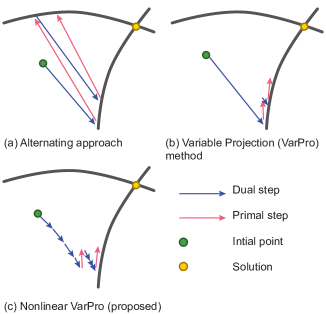
Figure 2: Comparison of (a) the alternating approach, (b) VarPro, and (c) the nonlinear VarPro proposed in the current paper.

4.1 VarPro with nonlinear iterative projection

Initialize $\alpha=0.1,\beta=0.05,\epsilon=1.0E-06,\epsilon_{2}=1.0E-07,\mathrm{n}=20,\mathrm{m}=160$

Initialize $\boldsymbol{x},\boldsymbol{y}$

while $\left\lVert J_{x}^{T}\boldsymbol{r}\right\lVert>\epsilon$ do

  $\mathrm{c}\leftarrow 0$

  while $(\left\lVert J_{y}^{T}\boldsymbol{r}\right\lVert>\epsilon_{2}\;\mathrm{and}\;\mathrm{c}<\mathrm{m})\;\mathrm{or}\;c<n$ do

   Update $J_{x}$,$J_{y}$, $\boldsymbol{r}$

   $\Delta\boldsymbol{y}\leftarrow D^{-1}J_{y}^{T}\boldsymbol{r}$

   $\boldsymbol{y}\leftarrow\boldsymbol{y}-\beta\Delta\boldsymbol{y}$

   $\mathrm{c}\leftarrow\mathrm{c}+1$

  end while

  Update $J_{x}$,$J_{y}$, $\boldsymbol{r}$

  $\Delta\boldsymbol{x}=(A-BD^{-1}C)^{-1}J_{x}^{T}\boldsymbol{r}$.

  $\boldsymbol{x}\leftarrow\boldsymbol{x}-\alpha\Delta\boldsymbol{x}$

end while

Algorithm 6 Nonlinear VarPro

The first idea we tested was to simply replace the dual step of VarPro with inner iterations that recursively solve the dual subproblem:

$$\frac{1}{2}\|\boldsymbol{r}(\boldsymbol{\bar{x}},\,\boldsymbol{y})\|^{2}\rightarrow\mathrm{min}.$$

As usual, the Gauss–Newton method was used to solve this subproblem with a small step size. These inner iterations were continued until the L2 norm of the gradient vector, $J_{y}^{T}\boldsymbol{r}$, reached a sufficiently small number before the primal step was executed.

However, the subsequent primal step was too unstable. This remained true even when the inner iterations were continued until the L2 norm of the gradient reached approximately 1.0E-10, which took over 400 steps.

The cause of the issue is that the computation of the correction vector, $\Delta\boldsymbol{x}=(A-BD^{-1}C)^{-1}J_{x}^{T}\boldsymbol{r}$, assumes that $J_{y}^{T}\boldsymbol{r}$ is strictly zero. In our nonlinear extension, $J_{y}^{T}\boldsymbol{r}$ cannot be rigorously zero by construction.

4.2 Gauss–Newton with nonlinear iterative projection

Initialize $\alpha=0.1,\beta=0.05,\epsilon=1.0E-07,\epsilon_{2}=1.0E-07,\mathrm{n}=20,\mathrm{m}=160$

Initialize $\boldsymbol{x},\boldsymbol{y}$

while $\left\lVert J_{x}^{T}\boldsymbol{r}\right\lVert>\epsilon$ do

  $\mathrm{c}\leftarrow 0$

  while $(\left\lVert J_{y}^{T}\boldsymbol{r}\right\lVert>\epsilon_{2}\;\mathrm{and}\;\mathrm{c}<\mathrm{m})\;\mathrm{or}\;c<n$ do

   Update $J_{x}$,$J_{y}$, $\boldsymbol{r}$

   $\Delta\boldsymbol{y}\leftarrow D^{-1}J_{y}^{T}\boldsymbol{r}$

   $\boldsymbol{y}\leftarrow\boldsymbol{y}-\beta\Delta\boldsymbol{y}$

   $\mathrm{c}\leftarrow\mathrm{c}+1$

  end while

  Update $J_{x}$,$J_{y}$, $\boldsymbol{r}$

  $\begin{pmatrix}\Delta\boldsymbol{x}\\[2.0pt] \Delta\boldsymbol{y}\end{pmatrix}=\begin{pmatrix}A&B\\[3.0pt] C&D\end{pmatrix}^{-1}\begin{pmatrix}J_{x}^{T}\,\boldsymbol{r}\\[2.0pt] J_{y}^{T}\,\boldsymbol{r}\end{pmatrix}$.

  $\boldsymbol{x}\leftarrow\boldsymbol{x}-\alpha\Delta\boldsymbol{x}$

end while

Algorithm 7 Nonlinear VarPro (Gauss–Newton ver)

Thus, we tested the Gauss–Newton method with a nonlinear iterative projection inserted at every step because this version can take into account a non-zero $J_{y}^{T}\boldsymbol{r}$. This method was the most reliable among all the strategies we tested. This means that the Gauss–Newton method is stable if $J_{y}^{T}\boldsymbol{r}$ is sufficiently small, although it is not rigorously zero. This makes total sense, as we assumed that the problem is separable into two mildly nonlinear subproblems; the problem should still be mildly nonlinear in the vicinity of the solution manifold of the dual subproblem.

The last remaining task is determining an adequate inner loop termination criterion. We initially anticipated that the total iteration count for the inner loop could be small–around 20. However, we eventually concluded that the L2-norm of the gradient of the dual subproblem must be sufficiently small after each projection. Hence, in our test, we targeted $1.0E-07$ for the L2-Norm of the gradient of the dual subproblem. This allows the L2-Norm of the gradient of the primal subproblem to decrease to at least $1.0E-06$. Additionally, the inner loop was continued until the minimum iteration count (20) and compulsorily terminated when the total iteration count reached the maximum iteration count (160).

5 Results

5.1 Sphere and Hemisphere

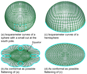
Figure 3: As conformal as possible flattening of a sphere (a,b) and a hemisphere (c,d). While strange wrinkles are formed around the equator of the sphere, a perfect conformal flattening is obtained for the hemisphere. This indicates that, while some surfaces have accurate conformal flattening with no singularities, some surfaces do not.

It is well known that a sphere can be conformally flattened if a small cut is introduced somewhere—at the south pole in this work. However, this is only true when the flattening can include singularities. Because NURBS surfaces cannot represent such singularities, a sphere is actually a good example of a surface that does not admit a conformal flattening if singularities are not permitted. Conversely, a hemisphere is a well-known example of a surface that does allow a conformal flattening without singularities. By solving the dual subproblem with the target surfaces fixed, one can easily confirm these, as shown in Fig. 3.

5.2 Examples with arbitrary geometry

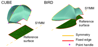
Figure 4: Two problems solved to test the proposed method.

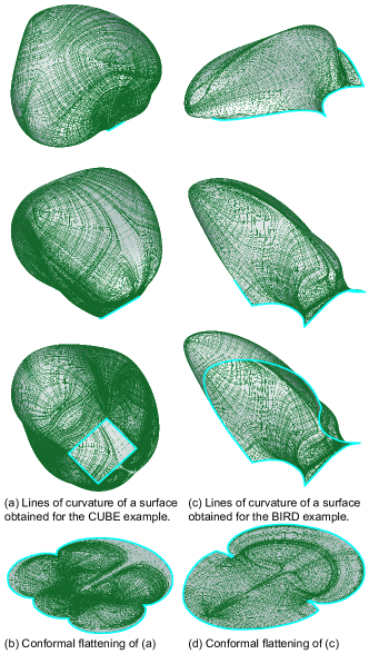
Figure 5: Obtained surfaces, their flattening, and lines of curvature using the proposed method. (a,b) a result for the CUBE example, (c,d) a result for the BIRD example.

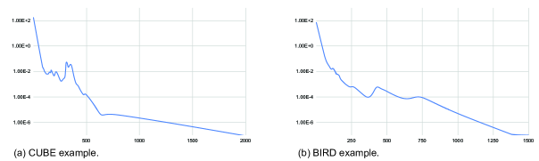
Figure 6: Plots illustrating the decrease in the L2-norm of the gradient vector of the primal subproblem. Note that the horizontal axis indicates the iteration count for the outer loop.

As shown in Fig. 4, we defined two simple problems, CUBE and BIRD, to test the proposed method. There are four NURBS patches with $9\times 9$ control points in the CUBE problem and three NURBS patches with $9\times 9$ control points in the BIRD example. We used degree 3 NURBS surfaces, which are also referred to as order 4 NURBS surfaces. The code was tested on a PC equipped with a Core i9-14900 CPU, an NVIDIA GeForce RTX 4090 GPU, and 128 GB of RAM. We used the CUDA Toolkit library®for the LU decomposition. We selected the variables for the target surface as the primal variables and those for the flattening as the dual variables.

The results are shown in Fig. 5. We also provide plots illustrating how the L2-norm of the gradient vector of the primal subproblem, $J_{x}^{T}\boldsymbol{r}$, decreases over iterations in Fig. 6.

We list the total computational time and iteration counts below:

1. For the CUBE problem, the computation took 2.5 hours until the L2-norm of the gradient vector of the primal subproblem decreased to approximately $1.0E-06$, which is approximately 160000 inner iterations and 1200 outer iterations.

2. For the BIRD problem, the computation took 2.0 hours until the L2-norm of the gradient vector of the primal subproblem decreased to approximately $1.0E-06$, which is approximately 160000 inner iterations and 1200 outer iterations.

6 Limitation and Discussion

Although the total iteration count is enormous, the biggest limitation stems from the assumption that the two subproblems are mildly nonlinear. Thus, while the original VarPro was relatively easy to implement due to its simple structure, this nonlinear extension requires expertise to formulate conditions in mildly nonlinear forms. While our experience is still limited, we consider

1. normalized vectors and tensors can make the problem highly nonlinear,

2. multiplication of several linear terms (i.e., partial derivatives) is permissible.

7 Conclusion

In this paper, we presented a NURBS-based approach for simultaneously refining and flattening a target doubly curved surface by ensuring that the target surface and its flattening are mutually conformal. This method was based on VarPro but extended so that it can solve nonlinear least-squares problems separable into two mildly nonlinear subproblems. We admit that the computational cost is excessive owing to the inner–outer loop structure of the proposed method. However, given the fantastic quality of the results, we believe this cost is justifiable.

References

- [1] Åke Björck. Numerical Methods for Least Squares Problems, volume 51. SIAM, 1996.
- [2] Åke Björck. Numerical methods for least squares problems. SIAM, 2024.
- [3] Mathieu Desbrun, Mark Meyer, and Pierre Alliez. Intrinsic parameterizations of surface meshes. In Computer graphics forum, volume 21, pages 209–218. Wiley Online Library, 2002.
- [4] Michael S Floater and Kai Hormann. Surface parameterization: a tutorial and survey. Advances in multiresolution for geometric modelling, pages 157–186, 2005.
- [5] Gene H Golub and Victor Pereyra. The differentiation of pseudo-inverses and nonlinear least squares problems whose variables separate. SIAM Journal on numerical analysis, 10(2):413–432, 1973.
- [6] Xianfeng Gu, Yalin Wang, Tony F Chan, Paul M Thompson, and Shing-Tung Yau. Genus zero surface conformal mapping and its application to brain surface mapping. IEEE transactions on medical imaging, 23(8):949–958, 2004.
- [7] Je Hyeong Hong, Christopher Zach, and Andrew Fitzgibbon. Revisiting the variable projection method for separable nonlinear least squares problems. In 2017 IEEE Conference on Computer Vision and Pattern Recognition (CVPR), pages 5939–5947, 2017.
- [8] Bruno Lévy, Sylvain Petitjean, Nicolas Ray, and Jérome Maillot. Least squares conformal maps for automatic texture atlas generation. ACM Trans. Graph., 21(3):362–371, July 2002.
- [9] Masaaki Miki and Toby Mitchell. Interactive exploration of tension-compression mixed shells. ACM Transactions on Graphics (TOG), 41(6), nov 2022.
- [10] Masaaki Miki and Toby Mitchell. Alignment conditions for nurbs-based design of grid shells. ACM Transactions on Graphics (TOG), 43(3), jul 2024.
- [11] Diane Valerie Ouellette. Schur complements and statistics. Linear Algebra and its Applications, 36:187–295, 1981.
- [12] Dianne P O’Leary and Bert W Rust. Variable projection for nonlinear least squares problems. Computational Optimization and Applications, 54:579–593, 2013.
- [13] Rohan Sawhney and Keenan Crane. Boundary first flattening. ACM Transactions on Graphics (ToG), 37(1):1–14, 2017.
- [14] Alla Sheffer and Eric de Sturler. Parameterization of faceted surfaces for meshing using angle-based flattening. Engineering with computers, 17:326–337, 2001.
- [15] Boris Springborn, Peter Schröder, and Ulrich Pinkall. Conformal equivalence of triangle meshes. In ACM SIGGRAPH 2008 papers, pages 1–11. 2008.
- [16] Fuzhen Zhang. The Schur complement and its applications, volume 4. Springer Science & Business Media, 2006.