Intermittent time series forecasting with Gaussian Processes and Tweedie likelihood

Abstract

We introduce the use of Gaussian Processes (GPs) for the probabilistic forecasting of intermittent time series. The model is trained in a Bayesian framework that accounts for the uncertainty about the latent function and marginalizes it out when making predictions. We couple the latent GP variable with two types of forecast distributions: the negative binomial (NegBinGP) and the Tweedie distribution (TweedieGP). While the negative binomial has already been used in forecasting intermittent time series, this is the first time in which a fully parameterized Tweedie density is used for intermittent time series. We properly evaluate the Tweedie density, which is both zero-inflated and heavy tailed, avoiding simplifying assumptions made in existing models. We test our models on thousands of intermittent count time series. Results show that our models provide consistently better probabilistic forecasts than the competitors. In particular, TweedieGP obtains the best estimates of the highest quantiles, thus showing that it is more flexible than NegBinGP.

[1]organization=SUPSI, Istituto Dalle Molle di Studi sull’Intelligenza Artificiale (IDSIA), city=Lugano, country=Switzerland

1 Introduction

Intermittent time series irregularly switch between zero and non-zero values. They characterize a large percentage of the inventory items and thus they represent an important element in the planning process (Johnston et al., 2003). Well-known forecasting methods for intermittent demand (Croston, 1972; Syntetos and Boylan, 2005; Nikolopoulos et al., 2011) only provide point forecasts. However, planning the inventory levels requires probability distributions (Boylan and Syntetos, 2021; Kolassa, 2016) from which to extract the relevant quantiles.

Probabilistic models for intermittent time series typically forecast the distribution of the demand (the positive values of the time series) and the probability of occurrence, i.e., the binary variable indicating whether there will be demand. Notable models include Hyndman et al. (2008, pp.281-283), Snyder et al. (2012), Sbrana (2023) and Svetunkov and Boylan (2023). All such models include one or more latent variables, related to the expected value of the demand or to the probability of occurrence.

The latent variables determine one or more parameters of the forecast distribution $p(y_{T+1}\mid y_{1:T})$, where $y_{1:T}$ are the observations available up to time $T$ and $y_{T+1}$ is the predicted value at time $T+1$. See Sec. 2 for more details. The above models consider a point estimate of the latent variables, without modeling their uncertainty. Yet, more accurate predictions can be obtained by accounting also for the uncertainty on the parameters of the forecast distribution (Prak and Teunter, 2019).

Our first contribution is to model the latent variable with a Gaussian Process (GP), a Bayesian non-parametric model which automatically quantifies the uncertainty of the latent variable and propagates it to the forecast distribution. GPs have already been applied for forecasting smooth time series (Roberts et al., 2013; Corani et al., 2021); we apply them for the first time to intermittent time series.

Another key aspect of modeling intermittent time series is that the forecast distribution needs a mass in zero. This can be achieved with a discrete distribution, such as the negative binomial (Harvey and Fernandes, 1989; Snyder et al., 2012; Kolassa, 2016). Our first model, NegBinGP, couples the Gaussian Process with a negative binomial distribution.

However, a unimodal forecast distribution can be restrictive. Indeed, often probabilistic models for intermittent time series have a bimodal distribution, with a point mass in zero and a distribution over positive values. We obtain a similar effect by coupling the GP with a Tweedie distribution (Dunn and Smyth, 2005), which is bimodal (with a mode in 0) and long-tailed. We call this model TweedieGP. To the best of our knowledge, this is the first application of a fully parameterized Tweedie distribution to intermittent time series. Indeed, properly evaluating the Tweedie distribution is not straightforward. In Sec. 3.2.1 we clarify how the Tweedie loss, often used for training point forecast models on intermittent time series (Jeon and Seong, 2022; Januschowski et al., 2022), is obtained by severely approximating the Tweedie distribution.

We perform experiments on about 40’000 supply chain time series from five different data sets. Thanks to variational methods (Hensman et al., 2015), the training times of GPs are in line with those of other methods for intermittent time series. Both GPs generally provide better probabilistic forecasts than the competitors. Importantly, TweedieGP outperforms NegBinGP (and all the other competitors) on the highest quantiles, the most important for inventory planning. This might be due to additional flexibility of the Tweedie distribution compared to the negative binomial.

We will release the implementation of our models and the instructions on how to replicate our experiments. Our implementation is based on GPyTorch (Gardner et al., 2018). Upon acceptance we will make available our code repository and we will release the Tweedie distribution as a class for PyTorch (Paszke et al., 2019), making it available for training more general probabilistic models.

2 Literature on probabilistic models for intermittent time series

Denoting the observation at time $t$ as $y_{t}$ and the indicator function as $\mathbbm{1}$, we obtain the occurrence and the demand at time $t$ as:

$$o_{t} :=\mathbbm{1}_{[y_{t}>0]},$$

$$d_{t} :=\begin{cases}y_{t}\ &\text{if}\ y_{t}>0\\ \text{undefined}&\text{otherwise.}\end{cases}.$$

Hyndman et al. (2008) propose a probabilistic version of Croston’s method (Croston, 1972), in which both the demand time series and the inter-demand intervals are predicted with two independent exponential smoothing processes. The probability of occurrence is obtained by inverting the estimated inter-demand intervals. As a result of having two latent processes, the forecast distribution is a mixture of a Bernoulli and a shifted Poisson.

Snyder et al. (2012) propose a model in which two latent independent exponential smoothing processes estimate the probability of occurrence and the demand. In this case, both simple and damped exponential smoothing are considered. Again, the forecast distribution is a mixture of a Bernoulli for $o_{t}$ and a shifted Poisson for $d_{t}$.

Snyder et al. (2012) also propose another model with a latent exponential smoothing that controls the mean of a negative binomial distribution. Thus the forecast distribution is unimodal and overdispersed.

Sbrana (2023), instead, models the time series with a latent process which can be equal to 0 with constant probability. The resulting forecast distribution is composed by a mass in zero and a truncated Gaussian distribution on the positive real line.

The iETS model (Svetunkov and Boylan, 2023) assumes the independence of occurrence and demand and models the latent variables via exponential smoothing. The latent demand variable is modelled as a multiplicative exponential smoothing process. iETS considers different models of occurrence, which are based on one or two exponential smoothing processes; they cover cases such as demand building up (the probability of occurrence increases over time), demand obsolescence, etc. The best occurrence model is chosen via AICc. The forecast distribution is the mixture of a Bernoulli and a Gamma distribution.

Similar models have been also implemented in a Bayesian fashion (Yelland, 2009; Chapados, 2014; Babai et al., 2021), with the advantage of propagating the uncertainty on the parameters of the forecast distribution. However, there is no readily available software implementation of them.

A non-parametric approach based on the independence between occurrence and demand is given by the WSS method (Willemain et al., 2004), which models the occurrence using a two-states Markov chain. When the simulated occurrence is positive, it samples the demand from past values of $d_{t}$, $t<T$, via bootstrapping with jittering. The resulting forecast distribution for $y_{T+1}$ is a mixture between a mass in 0 and an integer-valued, non-parametric distribution. A similar approach is also followed by Zhou and Viswanathan (2011).

Summing up, the most common choice is to independently model occurrence and demand, which results in a bimodal forecast distribution. However, demand intervals and demand levels have been found to be correlated (Altay et al., 2012).

However, if the time series contains a very large amount of zeros, static models might be preferable to time-series ones (Snyder et al., 2012). The static model might be constituted by the empirical quantiles (Boylan and Syntetos, 2021, Sec 13.2) or by a fitted parametric distribution such as the negative binomial (Kolassa, 2016).

3 Gaussian Processes

We model the dynamic of the latent variable with a Gaussian Process (GP, Rasmussen and Williams, 2006). A GP provides a prior distribution on the space of functions $f:\mathbb{R}_{+}\rightarrow\mathbb{R}$:

$$f\sim\mathcal{GP}\left(m(\cdot),k(\cdot,\cdot)\right),$$ (1)

where $m(\cdot)$ is a mean function and $k(\cdot,\cdot)$ is a positive definite kernel. We set $m(t)=c$ for all $t$, where $c\in\mathbb{R}$ is a learnable parameter.

We consider a training set of $T$ couples $(t_{1},y_{1}),\ldots,(t_{T},y_{T})$, where, for each $i$, $t_{i}$ is the time instance and $y_{i}$ is the time series observation. The training set does not need to be regularly spaced. We denote by $\mathbb{P}$ and $p$ probabilities and density functions respectively. The GP provides a prior on the latent vector $\mathbf{f}_{1:T}:=(f(t_{1}),\dots,f(t_{T}))^{\top}$ which is a multivariate Gaussian distribution:

$$p(\mathbf{f}_{1:T})=\mathcal{N}(\mathbf{f}_{1:T}\mid\mathbf{m}_{1:T},K_{T,T}).$$ (2)

As kernel, we use a Radial Basis Function (RBF):

$$k(t_{i},t_{j})=\theta^{2}\exp\left(-\frac{|t_{i}-t_{j}|^{2}}{2l^{2}}\right),$$

where the lengthscale $l\in\mathbb{R}_{+}$ and the outputscale $\theta\in\mathbb{R}_{+}$ are kernel hyper-parameters. The RBF kernel assumes $f$ to be a smooth function of time. The lengthscale determines how fast it changes in time: a smaller $l$ results in quicker variations of $f$. The outputscale instead controls the range of values attained by the latent function. See Rasmussen and Williams (2006, Chap. 4) for more details.

Samples of vectors $\mathbf{f}_{1:T}$ are shown in Fig. 1 (left). At time $t$, the $\gamma$-level credible interval is the interval that contains $\gamma$ $\%$ of values of $f_{t}$. A priori, the function has the same mean and variance at any time; hence the credible intervals are flat (Fig. 1, right).

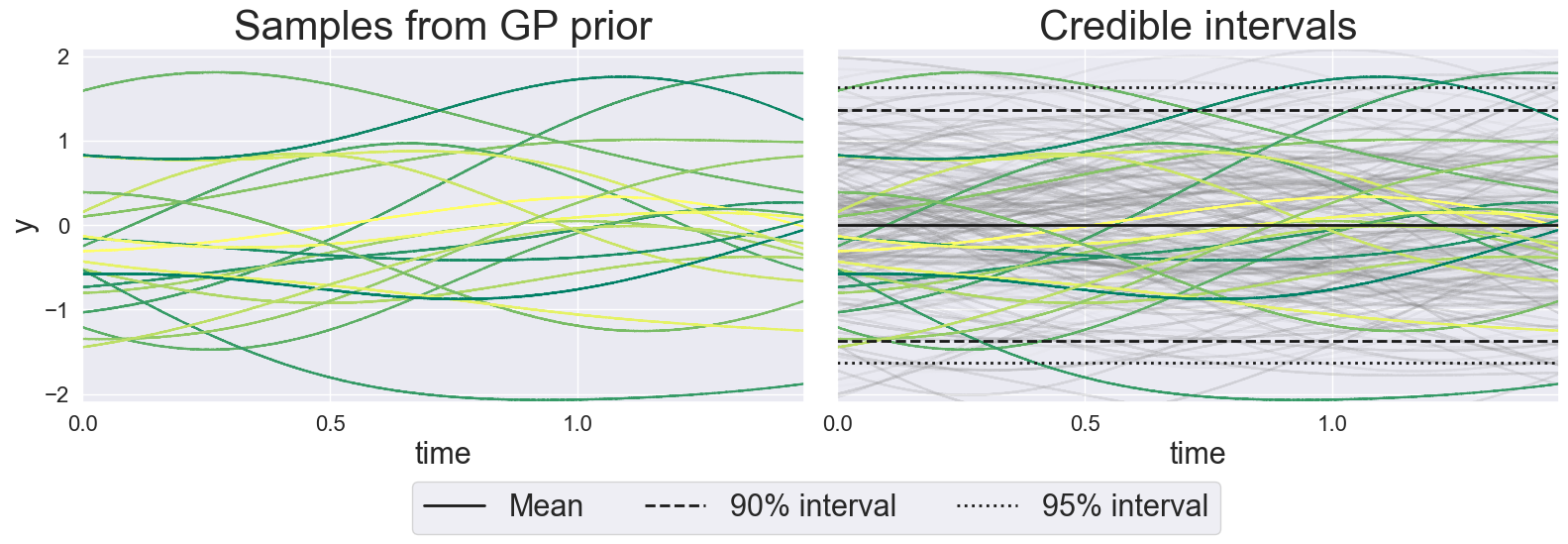
Figure 1: Sample trajectories drawn from the GP prior. The single trajectories fluctuate around the mean, while the credible intervals are flat.

We ensure the positivity of the latent function by passing it through the softplus function, defined as $\mathrm{softplus}(x):=\log(1+e^{x})$. The softplus maps negative values of $x$ to small positive values, while it is close to the identity function for $x>2$. A priori, the credible intervals of $\mathrm{softplus}(\mathbf{f}_{i})$ are identical for all time instants but also non-negative and asymmetric (Fig. 2, left).

Assuming the observations to be conditionally independent given the value of the latent function, the likelihood function is:

$$p(\mathbf{y}_{1:T}\mid\mathbf{f}_{1:T},\boldsymbol{\theta}_{\mathrm{lik}})=\prod_{i=1}^{T}p_{\mathrm{lik}}\left(y_{i}\mid\mathrm{softplus}(f_{i}),\boldsymbol{\theta}_{\mathrm{lik}}\right),$$ (3)

where $p_{\mathrm{lik}}(\cdot\mid\mathrm{softplus}(f_{i}),\boldsymbol{\theta}_{\mathrm{lik}})$ is either the negative binomial or the Tweedie distribution and $\boldsymbol{\theta}_{\mathrm{lik}}$ are their hyper-parameters, which we discuss in Secs. 3.1 and 3.2.

In a Bayesian framework, even after observing the training data, we have residual uncertainty about $\mathbf{f}_{1:T}$, described by its posterior distribution:

$$p(\mathbf{f}_{1:T}\mid\mathbf{y}_{1:T})\propto p(\mathbf{y}_{1:T}\mid\mathbf{f}_{1:T},\boldsymbol{\theta}_{\mathrm{lik}})p(\mathbf{f}_{1:T}),$$ (4)

as shown in the right panel of Fig. 2.

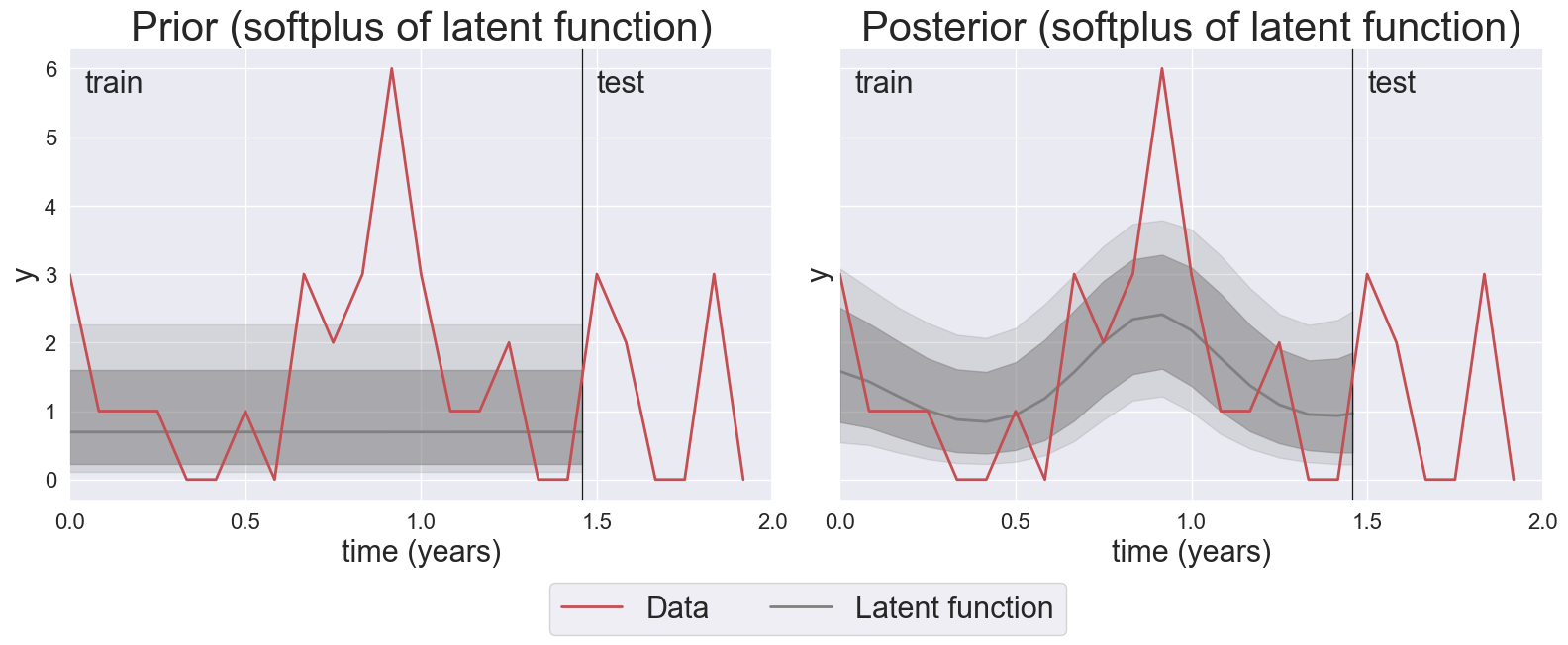
Figure 2: Prior (left) and posterior (right) distribution of the softplus of the GP latent function computed with a Tweedie likelihood. The shaded areas represent the 90% and 95% credible intervals. The vertical line divides train and test data. The data consist of the 1000-th time series from the Auto data set.

The posterior in eq. (4) is available in analytic form only for the Gaussian likelihood. Since our likelihoods are non-Gaussian, we approximate $p(\mathbf{f}_{1:T}~\mid~\mathbf{y}_{1:T})$ with a variational inducing point approximation (Hensman et al., 2013) constituted by a Gaussian density, denoted by $q(\mathbf{f}_{1:T}\mid\mathbf{y}_{1:T})$, with tunable mean and covariance parameters. We follow Hensman et al. (2015) to optimize the model parameters as described in A.

The distribution of the future values of the latent function, $\mathbf{f}_{T+1:T+h}=(f(t_{T+1}),\ldots,f(t_{T+h}))^{\top}$, is:

$$p(\mathbf{f}_{T+1:T+h}\mid\mathbf{y}_{1:T})=\int p(\mathbf{f}_{T+1:T+h}\mid\mathbf{f}_{1:T})q(\mathbf{f}_{1:T}\mid\mathbf{y}_{1:T})\mathrm{d}\mathbf{f}_{1:T},$$ (5)

where the integral is solved analytically since both $p$ and $q$ are Gaussian.

We obtain the forecast distribution by sampling from $p(\mathbf{f}_{T+1:T+h}\mid\mathbf{y}_{1:T})$ and passing each sample through the likelihood. Thus the uncertainty on $\mathbf{f}_{T+1:T+h}$ is propagated to the forecast distribution $p(\mathbf{y}_{T+1:T+h}~\mid~\mathbf{y}_{1:T})$. Fig. 3 shows the posterior distribution of $\mathbf{f}_{T+1:T+h}$ (left) and the forecast distribution (right).

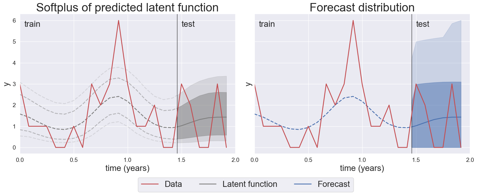
Figure 3: Example of TweedieGP forecasting. Left: posterior distribution of the GP latent function passed through the softplus. Right: forecast distribution using the Tweedie likelihood. The shaded regions represents $90\%$ and $95\%$ prediction intervals respectively. The figures complement the model fit in Fig. 2.

We now complete the GP model by specifying the likelihood function.

3.1 Negative binomial likelihood

We denote by $\mathrm{NegBin}(y;r,\text{p})$ the density of a negative binomial distribution with number of successes $r$ and success probability p. We set $r=\text{softplus}(f)$. Note that the mean and the variance of the distribution linearly increase with $r$. Instead, p is a hyper-parameter ($\boldsymbol{\theta}_{\mathrm{lik}}=\{\text{p}\}$), learned once via optimization and kept fixed for all the data points of the same time series.

The likelihood of an observation $y_{i}$ is:

$$p_{\mathrm{lik}}\left(y_{i}\mid\mathrm{softplus}(f_{i}),\boldsymbol{\theta}_{\mathrm{lik}}\right)=\mathrm{NegBin}(y_{i};\mathrm{softplus}(f_{i}),\text{p}).$$

3.2 The Tweedie likelihood

The Tweedie is a family of distributions (Dunn and Smyth, 2005) characterized by a power mean-variance relationship. A non-negative random variable $Y$ is distributed as a Tweedie, $Y\sim\mathrm{Tw}(\mu,\phi,\rho)$, if:

$$\mathrm{Var}[Y]=\phi\mu^{\rho},$$

where $\mu>0$ is the mean, $\rho>0$ is the power and $\phi>0$ is the dispersion parameter.

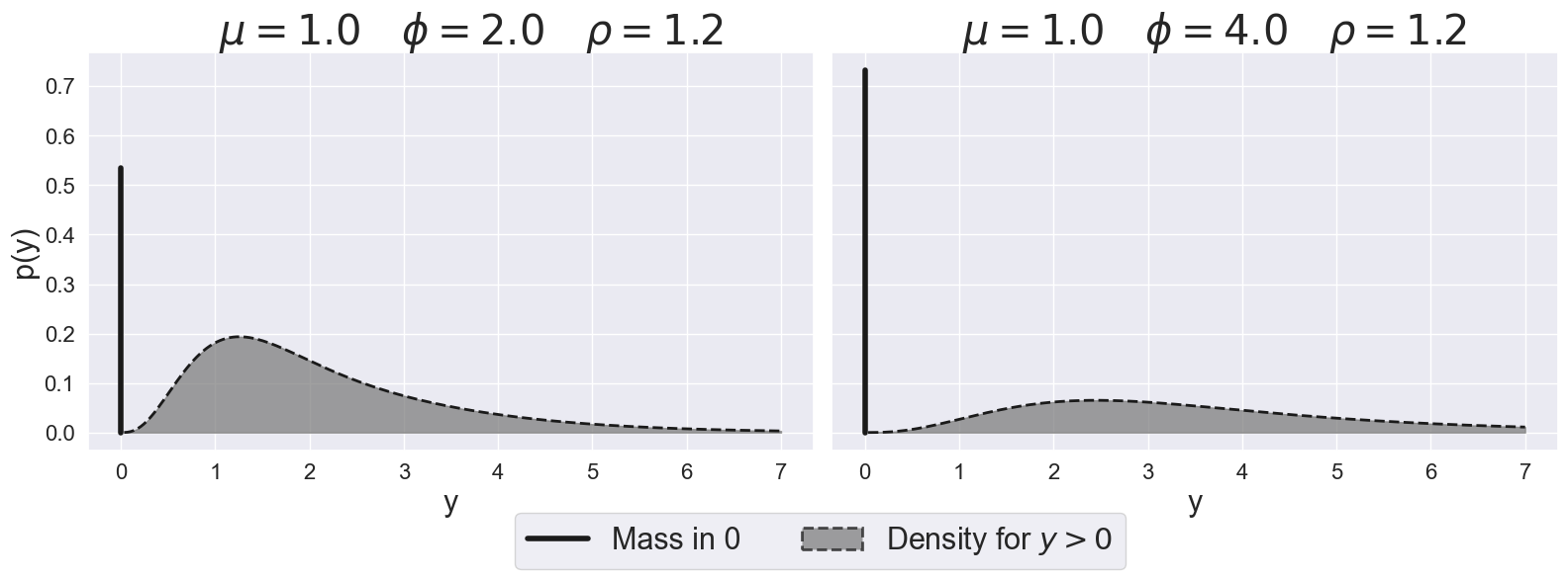
Figure 4: The Tweedie distribution is flexible and bimodal. The two distributions have the same mean, but the right one has higher dispersion ($\phi$). This results in a larger mass in 0 and in a longer right tail.

We assume $\rho\in(1,2)$, which allows interpreting the Tweedie (Dunn and Smyth, 2005) as a Poisson mixture of Gamma distributions:

$$Y \sim\sum_{i=0}^{N}X_{i},$$

$$X_{i} \overset{\mathrm{i.i.d.}}{\sim}\mathrm{Gamma}(\alpha,\beta),$$

$$N \sim\mathrm{Poisson}(\lambda),$$

with

$$\lambda=\frac{\mu^{2-\rho}}{\phi(2-\rho)},\quad\alpha=\frac{2-\rho}{\rho-1},\quad\beta=\frac{1}{\phi(\rho-1)\mu^{\rho-1}}.$$ (6)

The mass in 0 and the density for $y>0$ are:

$$\mathbb{P}(Y=0) =\mathbb{P}(N=0)=e^{-\lambda},$$ (7)

$$p(y\mid\lambda,\alpha,\beta) =\sum_{n=1}^{+\infty}e^{-\lambda}\frac{\lambda^{n}}{n!}\cdot\mathrm{Ga}(y\mid n\cdot\alpha,\beta),$$ (8)

where $\mathrm{Ga}(\cdot)$ is the density of a Gamma distribution. The Tweedie distribution is generally bimodal (Fig. 4): the first mode is in $0$, while the second one is the mode of the sum of Gamma distributions. The continuous density function on the positive real values can be adapted to count data by rounding.

The parametrization (7-8), though interpretable, is not usable as a likelihood function. Indeed there is no theoretical result for truncating the infinite sum in eq. (8) while controlling the exceedance probability. In order to evaluate the Tweedie we use the $(\mu,\phi,\rho)$ parametrization (Dunn and Smyth, 2005). The probability of zero and the continuous density for $y>0$ are:

$$\mathbb{P}(Y=0) =\exp\left(-\frac{\mu^{2-\rho}}{\phi(2-\rho)}\right),$$ (9)

$$p(y\mid\mu,\phi,\rho) =A(y)\cdot\exp\left[\frac{1}{\phi}\left(y\frac{\mu^{1-\rho}}{1-\rho}-\frac{\mu^{2-\rho}}{2-\rho}\right)\right],$$ (10)

with

$$A(y) =\frac{1}{y}\sum_{j=1}^{\infty}\frac{y^{j\alpha}(\rho-1)^{-j\alpha}}{\phi^{j(1+\alpha)}(2-\rho)^{j}j!\Gamma(j\alpha)}$$ (11)

$$=\frac{1}{y}\sum_{j=1}^{\infty}V(j),$$

where $\alpha$ is defined in eq. (6). Dunn and Smyth (2005) provide a truncating rule for evaluating the infinite summation of eq. (11). It exploits the fact that $V(j)$ is a concave function of $j$. In most cases only few terms of the summation need to be evaluated, as we show in B.1. The Tweedie distribution is thus difficult to implement; yet, once implemented, its evaluation only requires a small overhead compared to other distributions.

The likelihood of TweedieGP is thus obtained by substituting in eq. (3):

$$p_{\mathrm{lik}}\left(y_{i}\mid\mathrm{softplus}(f_{i}),\boldsymbol{\theta}_{\mathrm{lik}}\right)=\mathrm{Tw}(y_{i};\mathrm{softplus}(f_{i}),\phi,\rho),$$

where $\boldsymbol{\theta}_{\mathrm{lik}}=\{\phi,\rho\}$. We set $\mu=\text{softplus}(f)$. Thus the latent variable affects, through $\lambda$ and $\beta$, both the mass in $0$ and the distribution on the positive $y$, see eq. (6), (7), (8). We thus control a bimodal forecast distribution using a single latent process. The hyper-parameters $\phi$ and $\rho$ are optimized and they are equal for all the data points in the same time series.

We now discuss the relation between the Tweedie distribution and the Tweedie loss, often used to train point forecast models on intermittent time series.

3.2.1 Comparison with Tweedie loss

Januschowski et al. (2022) mentions the availability of the Tweedie loss for tree-based models as one of the reason of their good performance in the M5 competition. The Tweedie loss is indeed available both in lightGBM and in PyTorch Forecasting. Moreover, Jeon and Seong (2022) obtained good results in the M5 competition by training the DeepAR model (Salinas et al., 2020) with the Tweedie loss. Recall that all such models only return point forecasts.

The Tweedie loss (Jeon and Seong, 2022) is:

$$\mathcal{L}(\mu,\rho\mid y)=-y\frac{\mu^{1-\rho}}{1-\rho}+\frac{\mu^{2-\rho}}{2-\rho}.$$ (12)

Interpreting eq. (12) as a negative log-likelihood, the implied likelihood is:

$$p(y\mid\mu,\rho)=\exp\left(y\frac{\mu^{1-\rho}}{1-\rho}-\frac{\mu^{2-\rho}}{2-\rho}\right),$$ (13)

which approximates the Tweedie density in eq. (10) by setting both $A=1$ and $\phi=1$. Setting $A(y)=1$ avoids the evaluation of the infinite summation in eq. (11); however, this makes the distribution unimodal and shortens its tails. Indeed, $A$ is a function of $y$ and not a simple normalization constant. Moreover, fixing the dispersion parameter to $\phi=1$ further reduces the flexibility.

We can nevertheless understand why the function in eq. (12) is an effective loss function for point forecast on intermittent time series. The first term of the exponential corresponds to an unnormalised exponential distribution and the second term is a penalty term which forces $\mu$ to remain close to zero. We illustrate the shape of the unnormalized distribution eq. (13) in B.2.

In Sec. 4.6 we show that the accuracy of TweedieGP worsens when we train it by using the approximation with $A=1$, $\phi=1$ rather than the actual Tweedie distribution.

4 Experiments

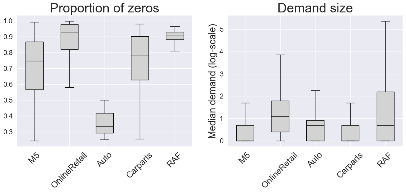
Figure 5: Proportion of zeros and mean demand in the different data sets. Notice that the y-axis of the median demand is in natural log scale.

Name	# of t.s.	Freq	T	h
M5	29003	Daily	1941	28
OnlineRetail	2023	Daily	333	31
Auto	1227	Monthly	18	6
Carparts	2499	Monthly	45	6
RAF	5000	Monthly	72	12

Table 1: Characteristics of the extracted intermittent time series. The data sets are from these domains: in-store sales, online sales, spare parts supply for cars and aircrafts.

We consider a time series as intermittent (Syntetos et al., 2005) if the mean interval between two positive demands (ADI) is larger than 1.32. By applying this criterion, we extract about 40’000 intermittent time series from the five data sets of Tab. 1. We show in Fig. 5 how the proportion of zeros and the demand size varies across the time series of each data set.

The data sets with the highest proportion of zeros (median $0.9$) are RAF and OnlineRetail (Fig. 5 left). An important difference is that the time series of OnlineRetail are about five times longer than those of RAF, Tab. 1. In contrast, Auto has the lowest proportion of zeros (median $0.35$) and its time series are also the shortest ($T=18$). The M5 data set is the most heterogeneous as for proportion of zeros and it generally has narrow demand. It also contains the largest amount (29’003) of time series, which are also very long ($T=1941$).

4.1 GP training

We implement our model in GPyTorch (Gardner et al., 2018). We estimate the variational parameters, the hyper-parameters of the GP ($c,l,\theta$) and of the likelihood (p for the negative binomial distribution, $\phi$ and $\rho$ for the Tweedie) via gradient descent for 100 iterations with early stopping, using Adam optimizer (Kingma and Ba, 2017) with learning rate $0.1$.

We train a GP for each time series. Its training time is generally comparable to state of the art methods for intermittent time series, as detailed in Sec. 4.5. Rarely, the training might fail due to numerical issues; when this happens, we restart the optimization. For both NegBinGP and TweedieGP, we obtain the forecast distribution by drawing 50’000 samples.

For TweedieGP, we scale the data by the median demand to ease the optimisation. This scaling can be applied as the zeroes remain unchanged and the Tweedie likelihood is absolutely continuous on positive data. We bring the samples back to the original scale after drawing them. We evaluate the effect of the scaling in Sec. 4.6.

4.2 Baselines

We compare NegBinGP and TweedieGP against 4 competitors. In order of complexity they are: empirical quantiles, WSS, ADIDA_C, and iETS.

The empirical quantiles (EmpQuant) assume the demand to be i.i.d. (Kolassa (2016), Boylan and Syntetos (2021, Sec 13.2)). The predicted quantiles are thus equal to the quantiles of the training set.

The WSS model (Willemain et al., 2004), already mentioned in Sec. 2, is a bootstrapping method which decomposes the time series into occurrence and demand. It models the dependence between occurrences using a two-states Markov chain. When the sampled occurrence is positive, it samples the demand from past values via bootstrapping with jittering. We developed our own implementation of WSS, drawing 50’000 samples for the forecast distribution.

We then consider the implementation of ADIDA (Nikolopoulos et al., 2011) provided by statsforecast (Garza et al., 2022), which we refer to ADIDA_C. ADIDA proceeds by temporally aggregating the intermittent time series. The aggregated time series are simpler to forecast as they contain fewer zeros. The predictions on aggregated time series, made with exponential smoothing, are then disaggregated to the original time buckets. While ADIDA is a point forecast method, ADIDA_C quantifies the uncertainty of the forecast via conformal inference (Angelopoulos and Bates, 2023); in order to obtain a non-negative distribution we perform a further step, assigning to zero all the mass on the negative values.

Finally, we use iETS (Svetunkov and Boylan, 2023) from the smooth package (Svetunkov (2024), v. 4.0.2). We use the most complete model (iETS_A) which fits four different occurrence models and selects among them via AICc.

In C, we show how to reproduce our experiments and we detail the integration of our models in GPyTorch (Gardner et al., 2018).

4.3 Metrics

Denoting by $\hat{y}_{q}$ the forecast of quantile $q$, and by $y$ the observed value, the quantile loss (Gneiting and Raftery, 2007) is:

$$\mathrm{Q}_{q}(\hat{y}_{q},y)=2\cdot\begin{cases}q(y-\hat{y}_{q})\quad&\text{if}\ y\geq\hat{y}_{q}\\ (1-q)(\hat{y}_{q}-y)\quad&\text{else}\end{cases}.$$ (14)

We evaluate $\mathrm{Q}_{q}(\hat{y}_{q},y)$ for the quantile levels $q\in\{0.5,0.8,0.9,0.95,0.99\}$. We do not assess quantiles lower than $0.5$ because they are generally estimated as zero by all models. For the same reason we do not report the Continuous Ranked Probability Score (CRPS), which averages the quantile loss over all quantiles.

The quantile loss is scale-dependent and thus it is not suitable to be averaged across time series. In order to obtain a scale-free indicator (Hyndman and Athanasopoulos, 2021, Sec 5.8) we scale it by the quantile loss of the empirical quantiles ($\mathrm{emp}_{q}$) on the training data:

$$\mathrm{sQ}_{q}(\hat{y}_{q},y)=\frac{\mathrm{Q}_{q}(\hat{y}_{q},y)}{\frac{1}{T}\sum_{t=1}^{T}\mathrm{Q}_{q}(\mathrm{emp}_{q},y_{t})}.$$

The scaled quantile loss values are usually greater than 1, since the scaling factor in the denominator, being based on the training set, is optimistically biased. For high levels of $q$, this metric strongly penalises cases in which $y$ exceeds the predicted value $\hat{y}_{q}$, that is, when the demand is underestimated.

We assess the estimated probability of zero demand and positive demand with the Brier score:

$$\mathrm{Br}(\hat{p},y)=(\mathbbm{1}_{[y>0]}-\hat{p})^{2},$$

where $\hat{p}\in[0,1]$ is the predicted probability of $y>0$.

Finally, we measure the forecast coverage, i.e., the proportion of observations that lie within the $(1-q)$ prediction interval. An ideal forecast has coverage $q$.

4.4 Discussion

Data set	Metric	EmpQuant	WSS	ADIDAC	iETS	NegBinGP	TweedieGP
M5	Br	0.23	0.23	0.22	0.20	0.20	0.20
	$\mathrm{sQ}_{0.5}$	1.88	1.87	1.88	1.82	1.78	1.79
	$\mathrm{sQ}_{0.8}$	1.74	1.77	1.46	1.67	1.48	1.46
	$\mathrm{sQ}_{0.9}$	1.57	1.65	1.35	1.70	1.29	1.26
	$\mathrm{sQ}_{0.95}$	1.39	1.51	1.37	1.97	1.19	1.16
	$\mathrm{sQ}_{0.99}$	1.25	1.40	1.69	3.23	1.16	1.16
OnlineRetail	Br	0.12	0.12	0.18	0.11	0.11	0.11
	$\mathrm{sQ}_{0.5}$	2.35	2.35	2.55	2.36	2.34	2.35
	$\mathrm{sQ}_{0.8}$	2.34	2.33	2.29	2.40	2.27	2.26
	$\mathrm{sQ}_{0.9}$	2.31	2.29	2.23	2.50	2.23	2.20
	$\mathrm{sQ}_{0.95}$	2.33	2.30	2.35	2.73	2.25	2.23
	$\mathrm{sQ}_{0.99}$	3.02	2.98	4.09	4.30	3.22	2.98
Auto	Br	0.25	0.26	0.29	0.25	0.25	0.25
	$\mathrm{sQ}_{0.5}$	1.15	1.36	1.19	1.17	1.14	1.14
	$\mathrm{sQ}_{0.8}$	1.30	1.53	1.34	1.36	1.29	1.28
	$\mathrm{sQ}_{0.9}$	1.48	1.65	1.59	1.52	1.42	1.42
	$\mathrm{sQ}_{0.95}$	1.84	1.84	2.21	1.74	1.65	1.62
	$\mathrm{sQ}_{0.99}$	4.32	2.57	7.51	3.16	2.45	2.56
Carparts	Br	0.17	0.16	0.19	0.15	0.15	0.16
	$\mathrm{sQ}_{0.5}$	1.13	1.15	1.20	1.09	1.10	1.11
	$\mathrm{sQ}_{0.8}$	1.18	1.33	1.14	1.15	1.10	1.09
	$\mathrm{sQ}_{0.9}$	1.25	1.45	1.16	1.27	1.16	1.13
	$\mathrm{sQ}_{0.95}$	1.32	1.63	1.34	1.54	1.17	1.19
	$\mathrm{sQ}_{0.99}$	1.86	1.99	3.72	3.11	1.65	1.56
RAF	Br	0.08	0.08	0.14	0.08	0.08	0.08
	$\mathrm{sQ}_{0.5}$	1.00	1.00	1.37	1.00	1.00	1.00
	$\mathrm{sQ}_{0.8}$	1.00	1.01	1.22	1.00	1.01	1.01
	$\mathrm{sQ}_{0.9}$	1.10	1.16	1.17	1.06	1.12	1.14
	$\mathrm{sQ}_{0.95}$	1.24	1.43	1.35	1.39	1.24	1.26
	$\mathrm{sQ}_{0.99}$	2.12	2.21	3.79	3.72	2.21	2.09

Table 2: Brier score and scaled quantile loss (mean over $h$ and data set).

We show in Tab. 2 the mean score of each method on each data set. The mean is taken with respect to both the forecast horizons ($1,2,\ldots,h$) and all the time series of the data sets. As already discussed, the scaled quantile loss ($\mathrm{sQ}_{q}$) takes large values when the observation is beyond the predicted quantile. This rarely occurs with high quantiles, but these cases are relevant for decision making. We thus report the mean of $\mathrm{sQ}_{q}$ rather than its median, which would overlook those cases.

In each row we boldface the model with the lowest loss and the models whose loss is not significantly different from the best. We test significance of the difference in loss by using the paired $t$-test with FDR correction for multiple comparisons (Hastie et al., 2009, Sec 18.7.1).

An important finding is that TweedieGP is almost always the best performing model on the highest quantiles $\{0.9,0.95,0.99\}$ , arguably the most important for decision making. Its advantage over the other methods on the highest quantiles might be due to Tweedie distribution’s ability to extend its tails.

More in details, TweedieGP and NegBinGP tend to perform similarly on data sets containing short time series (Auto, Carparts, RAF). Indeed, when few training data is available, the effect of the GP prior might be more important than the choice of the likelihood. In contrast, on data sets containing longer time series (OnlineRetail, M5), TweedieGP has generally an advantage over NegBinGP. The advantage of TweedieGP on the highest quantiles is for instance emphasized on OnlineRetail, whose time series are both long and with high demand (see Fig. 5), challenging the long tails of the forecast distribution.

iETS matches the performance of NegBinGP and TweedieGP on the Brier score and on the median quantile, where the performance of all methods is closer, but it is often outperformed on the highest quantiles. This is in line with the results reported by Svetunkov and Boylan (2023), in which iETS was not the best performing approach on the highest quantiles.

The generally poor performance of ADIDA_C is most likely due to the inadequacy of conformal inference for count data. Indeed, the empirical quantiles are generally preferable to both WSS and ADIDA_C. In particular on the RAF data set, which is characterized by the largest amount of zeros, the empirical quantiles match the performance of the GPs. This confirms the suitability of static models for very sparse time series; it also shows that the GP latent function adapts well to different types of temporal correlations, becoming also an i.i.d model when needed.

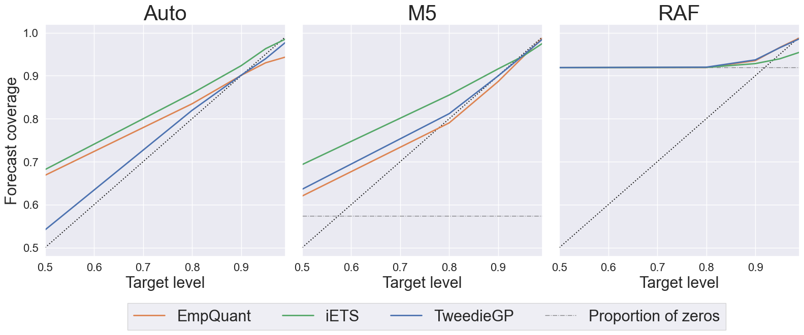
Figure 6: The coverage cannot go below the proportion of zeros in the test set, shown by a dashed horizontal line. On RAF, this implies overcoverage of most quantiles, apart from the highest ones.

Fig. 6 shows the calibration of selected methods (empirical quantiles, iETS and TweedieGP) on three data sets (Auto, M5 and RAF). Better forecasts lie closer to the dotted diagonal line. On intermittent time series, the coverage is at least as large as the proportion of zeros; there is hence overcoverage of the lower quantiles, as clear from the third panel of Fig. 6.

On the Auto data set, which has moderate intermittency, TweedieGP is the only one to have almost correct coverage on all quantiles above $0.5$. A similar comment can be done for M5, even though in this case the proportion of zeros is larger. Correct coverage is provided, only by TweedieGP and empirical quantiles, for quantiles above $0.8$. On the RAF data set, the very sporadic demand implies forecast overcoverage apart from the highest quantiles.

It is also interesting to analyze how the models compare on the quantile loss when they are correctly calibrated. For instance, empirical quantiles, iETS and TweedieGP provide correct coverage on the 95-th quantile of M5. On Auto, both TweedieGP and the empirical quantiles provide correct coverage on the 90-th quantile. In these cases, TweedieGP provides the lowest quantile loss (Tab. 2) among correctly calibrated models. Recall that the quantile loss combines a reward for the sharpness and a miscoverage penalty. Hence, given the same calibration, TweedieGP achieves lower loss as it provides a sharper estimate of the quantiles.

4.5 Computational times

Data set	WSS	ADIDAC	iETS	NegBinGP	TweedieGP
Auto	$0.04\pm 0.02$	$0.01\pm 0.01$	$0.13\pm 0.03$	$0.20\pm 0.06$	$0.20\pm 0.08$
RAF	$0.05\pm 0.03$	$0.01\pm 0.01$	$0.20\pm 0.03$	$0.22\pm 0.06$	$0.30\pm 0.07$
M5	$0.10\pm 0.03$	$0.01\pm 0.01$	$0.76\pm 0.07$	$1.20\pm 0.39$	$2.12\pm 0.49$

Table 3: Mean and standard deviation of the time (seconds) for training the models and generating forecasts. Experiments are run on the CPU of a M3 MacBook Pro.

We report in Tab. 3 the computational times of each method, including training and generating the forecasts on time series of selected data sets, ordered from the shortest to the longest (see Tab. 1). ADIDA_C and WSS are the fastest, with an average training time of 0.1 sec. or less.

The computational time of our methods is comparable with that of iETS. On the data sets containing the longest time series (M5), the average computational time of the GPs is about 2 seconds. This is noteworthy: an exact GP implementation would be rather slow on the time series of the M5 data set, due to its cubic computational complexity in the number of observations $T$. Thanks to the variational approximation, the computational complexity of our models is instead quadratic in $T$ for $T<200$. For longer time series the cost is capped by the variational formulation and becomes linear in $T$. See A for a more detailed evaluation.

The computational times of TweedieGP and NegBinGP are close; the fully parameterised Tweedie density only implies a small overhead compared to the negative binomial. On the M5 data set, NegBinGP is faster than TweedieGP as it often meets the early stopping condition.

4.6 Ablation study

In this section we evaluate TweedieGP against two simpler models: a GP model trained with the approximate Tweedie likelihood with $A=\phi=1$ (implied by the Tweedie loss) and a TweedieGP trained on unscaled data. We keep the same experimental setup of the previous section and we show the results in Tab. 4.

Data set	Metric	Non-scaled Tweedie	Tweedie $A=\phi=1$	Tweedie
M5	Br	0.20	0.20	0.20
	$\mathrm{sQ}_{0.5}$	1.79	1.80	1.79
	$\mathrm{sQ}_{0.8}$	1.46	1.47	1.46
	$\mathrm{sQ}_{0.9}$	1.27	1.30	1.26
	$\mathrm{sQ}_{0.95}$	1.17	1.23	1.16
	$\mathrm{sQ}_{0.99}$	1.17	1.37	1.16
OnlineRetail	Br	0.12	0.13	0.11
	$\mathrm{sQ}_{0.5}$	2.35	2.43	2.35
	$\mathrm{sQ}_{0.8}$	2.29	2.32	2.26
	$\mathrm{sQ}_{0.9}$	2.26	2.25	2.20
	$\mathrm{sQ}_{0.95}$	2.35	2.32	2.23
	$\mathrm{sQ}_{0.99}$	3.39	3.39	2.98
Auto	Br	0.25	0.25	0.25
	$\mathrm{sQ}_{0.5}$	1.15	1.13	1.14
	$\mathrm{sQ}_{0.8}$	1.28	1.30	1.28
	$\mathrm{sQ}_{0.9}$	1.43	1.44	1.42
	$\mathrm{sQ}_{0.95}$	1.66	1.65	1.62
	$\mathrm{sQ}_{0.99}$	2.80	2.58	2.56
Carparts	Br	0.15	0.16	0.16
	$\mathrm{sQ}_{0.5}$	1.10	1.11	1.11
	$\mathrm{sQ}_{0.8}$	1.09	1.10	1.09
	$\mathrm{sQ}_{0.9}$	1.16	1.13	1.13
	$\mathrm{sQ}_{0.95}$	1.22	1.20	1.19
	$\mathrm{sQ}_{0.99}$	1.73	1.59	1.59
RAF	Br	0.11	0.10	0.08
	$\mathrm{sQ}_{0.5}$	1.02	1.03	1.00
	$\mathrm{sQ}_{0.8}$	1.10	1.15	1.01
	$\mathrm{sQ}_{0.9}$	1.23	1.19	1.14
	$\mathrm{sQ}_{0.95}$	1.36	1.26	1.26
	$\mathrm{sQ}_{0.99}$	2.43	2.25	2.09

Table 4: Comparison of GP model with different likelihoods; all models use the RBF kernel.

The accuracy of TweedieGP is generally worse if we do not scale of the demand. Due to numerical issues, the posterior mean of the Gaussian process does not grow over a certain threshold, which is problematic when demand becomes high.

Finally, the performance of the approximated Tweedie likelihood with $\phi=A=1$ confirms what discussed in Sec. 3.2.1: the Tweedie loss might produce effective point forecasts by penalizing values far from zero, but the shorter tails negatively affect the estimate of the higher quantiles.

5 Conclusions

The two proposed Gaussian Process models provide state-of-the-art performance for intermittent time series forecasting. The Tweedie distribution is an interesting alternative to the negative binomial as a forecast distribution, being bimodal and allowing an accurate estimation of the highest quantiles.

In this paper we considered local models, trained on a single time series. In future it could be interesting to train also probabilistic global models (Montero-Manso and Hyndman, 2021; Salinas et al., 2020; Seeger et al., 2016) on intermittent time series with the Tweedie forecast distribution.

We only used a simple RBF kernel; in future works, we could test kernels composition (Rasmussen and Williams, 2006, Chap.4) in order to model the effect of seasonality or of covariates (Corani et al., 2021).

Appendix A Learning a sparse variational GP with a Tweedie likelihood

Recall that our forecasting model learns the posterior of the latent function $\mathbf{f}_{1:T}$ given the observations. The prior for a latent vector of length $T$ (training data length) is $p(\mathbf{f}_{1:T})=\mathcal{N}(\mathbf{f}_{1:T}\mid\mathbf{0},K_{T,T})$ and the joint distribution of data and latent variables is

$$p(\mathbf{y}_{1:T},\mathbf{f}_{1:T})=\prod_{i=1}^{T}\mathrm{Tw}(y_{i};\mathrm{softplus}(f_{i}),\phi,\rho)\mathcal{N}(\mathbf{f}_{1:T}\mid\mathbf{0},K_{T,T})$$ (15)

The posterior over latent function $p(\mathbf{f}_{1:T}\mid y_{1:T})$ is not available analytically therefore we need to approximate it. Moreover, in order to optimise the hyperparameters of the model, we also need to approximate the marginal likelihood $p(\mathbf{y}_{1:T})$. We follow Hensman et al. (2015) and use a sparse GP model with inducing points.

We proceed by augmenting our GP model with additional $m$ input-output pairs $\mathbf{Z}$, $\mathbf{u}$ that are distributed as the GP $f$, i.e. the joint distribution of the vector $(\mathbf{f}_{1:T},\mathbf{u})$ is

$$p(\mathbf{f}_{1:T},\mathbf{u})=\mathcal{N}\left(\begin{bmatrix}\mathbf{f}_{1:T}\\ \mathbf{u}\end{bmatrix}\ \Bigg{|}\ \mathbf{0},\begin{bmatrix}K_{T,T}&K_{T,m}\\ K_{m,T}&K_{m,m}\end{bmatrix}\right),$$

where $K_{m,m}$ and $K_{T,m}$ are the covariance matrices resulting from evaluating the kernel $k$ at the input values. Note that the Gaussian assumption implies that $p(\mathbf{f}_{1:T}\mid\mathbf{u})$ is available analytically via Gaussian conditioning.

The joint distribution of data and latent variables thus becomes $p(\mathbf{y}_{1:T},\mathbf{f}_{1:T},\mathbf{u})=p(\mathbf{y}_{1:T}\mid\mathbf{f}_{1:T})p(\mathbf{f}_{1:T}\mid\mathbf{u})p(\mathbf{u})$. We consider the approximate distribution $q(\mathbf{u})=\mathcal{N}(\mathbf{u}\mid\mathbf{m},\mathbf{S})$, where $\mathbf{m},\mathbf{S}$ are free parameters to be optimized.

In variational inference we assume that the posterior is approximated by $p(\mathbf{f}_{1:T}\mid\mathbf{y}_{1:T})\approx q(\mathbf{f}_{1:T}\mid\mathbf{y}_{1:T})=\int p(\mathbf{f}_{1:T}\mid\mathbf{u})q(\mathbf{u})d\mathbf{u}$. Since $q(\mathbf{u})$ is Gaussian we can solve the integral analytically. We can then bound the marginal log-likelihood $\log p(\mathbf{y}_{1:T})$ with the standard variational bound (Hensman et al., 2013)

$$\log p(\mathbf{y}_{1:T})\geq\mathbb{E}_{q(\mathbf{u})}[\log p(\mathbf{y}_{1:T}\mid\mathbf{u})]-\mathrm{KL}[q(\mathbf{u})\mid p(\mathbf{u})],$$

which can be further bounded as

$$\log p(\mathbf{y}_{1:T})\geq\mathbb{E}_{q(\mathbf{f})}[\log p(\mathbf{y}_{1:T}\mid\mathbf{f})]-\mathrm{KL}[q(\mathbf{u})\mid p(\mathbf{u})].$$ (16)

The right-hand side of eq. (16) is the evidence lower bound (ELBO). This is a loss function that can be used to optimize the model hyper-parameters ($c,l,\theta,\phi,\rho$), the location of the inducing points ($\mathbf{Z}$) and the variational parameters ($\mathbf{m},\mathbf{S}$).

The KL part of the ELBO is available analytically, however the expectation part needs an implementation of the log-likelihood function. The expectation is then evaluated with Monte Carlo sampling by exploiting the fact that $q(\mathbf{f})$ is a Gaussian distribution with known parameters.

We implemented the log-likelihood function $\log p(\mathbf{y}_{1:T}\mid\mathbf{f})$ for the Tweedie likelihood and then used the GPyTorch infrastructure (Gardner et al., 2018), for optimizing the ELBO.

Given the optimized variational posterior approximation $q(\mathbf{f}_{1:T}\mid\mathbf{y}_{1:T})$, we can compute the predictive latent distribution $h$-step ahead as

$$p(\mathbf{f}_{T+1:T+h})=\int p(\mathbf{f}_{T+1:T+h}\mid\mathbf{f}_{1:T})q(\mathbf{f}_{1:T}\mid\mathbf{y}_{1:T})\mathrm{d}\mathbf{f}_{1:T},$$ (17)

note that this integral has an analytic solution because the distributions are both Gaussian therefore $\mathbf{f}_{T+1:T+h}$ is a multivariate Gaussian distribution with known mean and covariance; see, e.g., Hensman et al. (2015) for detailed formulas.

The predictive posterior for the observations is computed by extracting samples $\mathbf{\tilde{f}}^{(j)}$, $j=1,\ldots,N$, from the distribution in eq. (17). For each sample $\mathbf{\tilde{f}}^{(j)}$, we draw one sample from

$$p(\mathbf{y}_{T+1:T+h}\mid\mathbf{\tilde{f}}^{(j)}_{T+1:T+h})=\prod_{i=T+1}^{T+h}p_{\mathrm{lik}}\left(y_{i};\mathrm{softplus}(\tilde{f}^{(j)}_{i}),\phi,\rho\right)$$

to obtain a sample from the predictive posterior.

In our experiments we choose the number of inducing points as follows. On short time series ($T\leq 200$), we use $T$ inducing points and initialize their locations in correspondence of the training inputs. On longer time series ($T>200$) we use $200$ inducing points, sampling their initial locations from a multinomial distribution with $p(i)\propto\log\left(1+\frac{i}{T}\right)$, $i=1,\ldots,T$. Thus the recent observations, which are more relevant for forecasting, have higher probability of being chosen as initial location of the inducing points. Since the method has a quadratic cost in $m$, the number of inducing points, and it is linear in $T$, the size of the training set, then we achieve quadratic cost in $T$ for $T<200$ and linear cost in $T$ for $T>200$.

All the steps outlined here are also valid for a negative binomial likelihood, once the joint distribution in eq. (15) is written with the negative binomial likelihood.

Appendix B Evaluation of the Tweedie density

B.1 Truncating the infinite summation

In Sec. 3.2 we show that, given $\mu>0$, $\phi>0$ and $\rho\in(1,2)$ the Tweedie density is

$$p(y\mid\mu,\phi,\rho)=\begin{cases}\exp(-\frac{\mu^{2-\rho}}{\phi(2-\rho)})&\text{if}\ y=0;\\ A(y)\cdot\exp\left[\frac{1}{\phi}\left(y\frac{\mu^{1-\rho}}{1-\rho}-\frac{\mu^{2-\rho}}{2-\rho}\right)\right]&\text{otherwise}\end{cases}$$ (18)

where

$$A(y) =\frac{1}{y}\sum_{j=1}^{\infty}\frac{y^{j\alpha}(\rho-1)^{-j\alpha}}{\phi^{j(1+\alpha)}(2-\rho)^{j}j!\Gamma(j\alpha)}$$

$$=\frac{1}{y}\sum_{j=1}^{\infty}V(j)\quad\text{with}\ \alpha=\frac{2-\rho}{\rho-1}$$ (19)

Dunn and Smyth (2005) evaluate $A(y)$ by approximating the infinite sum in eq. (19) with a finite one, retaining its largest elements. We start by finding

$$j_{\mathrm{max}}=\operatorname*{arg\,max}_{j\in\mathbb{N}}V(j),$$

which is the index of the largest component. To identify it, let

$$z=\frac{y^{\alpha}(\rho-1)^{-\alpha}}{\phi^{1+\alpha}(2-\rho)},$$ (20)

then

$$V(j)=\frac{z^{j}}{j!\Gamma(\alpha j)}$$

and

$$\log V(j)=j\log z-\log\Gamma\left(1+j\right)-\log\Gamma\left(\alpha j\right).$$ (21)

Stirling’s approximation allows us to simplify the evaluation of the Gamma function: $\Gamma(x+1)\simeq\sqrt{2\pi x}\cdot x^{x}\cdot e^{-x}$. Therefore

$$\log\Gamma(x+1)\simeq\frac{1}{2}\log 2\pi+\frac{1}{2}\log x+x\log x-x.$$ (22)

Approximating $\Gamma(\alpha j)$ with $\Gamma(1+\alpha j)$ in eq. (21) and using eq. (22) we have

$$\log V(j)\simeq j\log z-\frac{1}{2}\log 2\pi-\frac{1}{2}\log j-j\log j+j-\frac{1}{2}\log 2\pi$$ (23)

$$-\frac{1}{2}\log\alpha-\frac{1}{2}\log j-\alpha j\log\alpha-\alpha j\log j+\alpha j$$

$$= j\left(\log z+(1+\alpha)-\alpha\log\alpha-(1+\alpha)\log j\right)$$ (24)

$$-\log 2\pi-\frac{1}{2}\log\alpha-\log j.$$ (25)

Differentiating with respect to $j$ we have

$$\frac{\partial\log V(j)}{\partial j}\simeq \log z+(1+\alpha)-\alpha\log\alpha-(1+\alpha)\log j-j(1+\alpha)\frac{1}{j}-\frac{1}{j}$$

$$= \log z-\log j-\alpha\log(\alpha j)-\frac{1}{j}$$

$$\simeq \log z-\log j-\alpha\log(\alpha j)$$ (26)

which is a monotone decreasing function of $j$. For this reason, $\log V$ is a convex function (and therefore $V$ too). To identify its maximum point, we equate it to $0$ obtaining

$$(1+\alpha)\log j_{\mathrm{max}}=\log z-\alpha\log\alpha$$ (27)

and substituting $z$ from eq. (20) and $\alpha$ from eq. (19)

$$j_{\mathrm{max}}^{1+\alpha} =\frac{y^{\alpha}(\rho-1)^{-\alpha}}{\phi^{1+\alpha}(2-\rho)}\cdot\frac{(2-\rho)^{-\alpha}}{(\rho-1)^{-\alpha}}$$

and finally, since $\frac{\alpha}{1+\alpha}=2-\rho$:

$$j_{\mathrm{max}}=\frac{y^{2-\rho}}{\phi(2-\rho)},$$ (28)

where it can be appropriately rounded to be a natural number. Substituting $j_{\mathrm{max}}$ into $V$ using eq. (27), it gives

$$\log V(j_{\mathrm{max}})=j_{\mathrm{max}}(1+\alpha)-\log 2\pi-\log j_{\mathrm{max}}-\frac{1}{2}\log\alpha$$ (29)

From this point, one can start evaluating $V(j)$ for $j=j_{\mathrm{max}}+1,j_{\mathrm{max}}+2,\dots$, until a value $j_{U}$ is found, such that

$$\frac{V(j_{\mathrm{max}})}{V(j_{U})}\geq e^{37}$$

To compute that, one can either evaluate the difference between eqs. (21) and (29) or compute, again using eq. (21)

$$\log V(j_{\mathrm{max}})-\log V(j_{U})\simeq(j_{\mathrm{max}}-j_{U})C_{W}-\left(j_{\mathrm{max}}\left(1+\alpha\right)+1\right)\log j_{\mathrm{max}}+\left(j_{U}\left(1+\alpha\right)+1\right)\log j_{U}$$ (30)

where $C_{W}=\log z+(1+\alpha)-\alpha\log\alpha$ does not depend on $j$; such expression can be computed efficiently. Similarly, one can identify $j_{L}$ such that

$$\frac{V(j_{\mathrm{max}})}{V(j_{L})}\geq e^{37}$$

going backwards to $j_{\mathrm{max}}-1,j_{\mathrm{max}}-2$, potentially stopping at $j=1$. The fact that $\log V$ is a convex function implies that the value of $V$ decreases exponentially on both sides. Hence, the truncated part of the summation can be bounded with geometric sums:

$$\sum_{j=1}^{+\infty}V(j)-\sum_{j=j_{L}}^{j_{U}}V(j)\leq V\left(j_{L}-1\right)\frac{1-r_{L}^{j_{L}-1}}{1-r_{L}}+V\left(j_{U}+1\right)\frac{1}{1-r_{U}}$$

where

$$r_{L}=\exp\left(\frac{\partial\log V(j)}{\partial j}\right)\biggr{\rvert}_{j=j_{L}-1}\quad\mathrm{and}\quad r_{U}=\exp\left(\frac{\partial\log V(j)}{\partial j}\right)\biggr{\rvert}_{j=j_{U}+1}$$

The treshold $e^{-37}$ has been proposed since $e^{-37}\simeq 8\cdot 10^{-17}$ guarantees an appropriate precision using 64-bit floating points. See Dunn and Smyth (2005) for more. In practice, we are interested in computing the log-likelihood

$$\log p(y\mid\mu,\phi,\rho)=\log A(y)\left[\frac{1}{\phi}\left(y\frac{\mu^{1-\rho}}{1-\rho}-\frac{\mu^{2-\rho}}{2-\rho}\right)\right]$$

which similarly requires to pass $A(y)$ trough the logarithm. To efficiently implement the evaluation of $A$, it sufficient to refer to eqs. (19), (21), (28), (29), and (30).

	$\phi$	0.5					1.0					2.0					5.0
	$\rho$	1.01	1.1	1.2	1.3	1.5	1.01	1.1	1.2	1.3	1.5	1.01	1.1	1.2	1.3	1.5	1.01	1.1	1.2	1.3	1.5
$y$	0.1	2	3	5	7	14	2	2	4	6	10	2	2	3	5	8	2	2	3	4	6
	0.2	2	4	6	9	15	2	3	5	7	11	2	2	4	5	9	2	2	3	4	7
	0.5	3	6	9	12	18	2	4	6	8	14	2	3	5	6	10	2	2	4	5	8
	0.8	4	7	11	14	21	2	5	8	10	15	2	3	5	7	11	2	2	4	5	8
	1	5	9	12	14	21	3	6	9	11	16	2	4	6	8	12	2	3	4	6	9
	1.5	5	10	14	17	24	4	7	9	12	18	2	5	7	9	14	2	3	5	6	9
	2	5	12	16	19	26	5	8	11	14	18	3	6	8	10	14	2	3	5	7	10
	5	7	19	24	27	33	6	12	16	18	23	5	9	11	13	17	2	5	7	8	11
	10	9	25	32	36	40	7	18	21	24	28	6	12	14	16	20	4	7	9	11	14

Table 5: $j_{U}-j_{L}+1$ for different choices of $y$, $\phi$ and $\rho$. This is the amount of terms used in the approximation of the summation. It is an increasing function with respect to $y$ and $\rho$, decreasing with respect to $\phi$.

Figure 7: The values of $\phi$ and $\rho$ on the fitted TweedieGP on different data sets. Density curves have been estimated via kernel density estimation.

Table 5 shows the amount of terms in the approximation of the summation $A$ is generally affordable; indeed scaling the data by median demand, the value of $y$ typically lies between 0.5 and 2, while the density plots from Fig. 7 show that often $\phi\in(0.5,5)$ with mode around 1, and $\rho\in(1,1.4)$, with mode around $1.1$.

B.2 Comparison with Tweedie loss

In order to consider the crucial role of $A$ in fitting appropriately a Tweedie likelihood to the data, consider again the Tweedie loss, characterised by $\phi=A=1$: in this simplified version, the implied likelihood in eq. (13) is no longer a probability distribution, as it does not integrate up to $1$. If constrained to do so determining $c:=c(\mu,\phi,\rho)$ such that

$$\int_{0}^{+\infty}c\cdot\exp\left(y\frac{\mu^{1-\rho}}{1-\rho}-\frac{\mu^{2-\rho}}{2-\rho}\right)dy=1$$

including the normalization constant $c=\frac{\mu^{1-\rho}}{\rho-1}\exp\left(\frac{\mu^{2-\rho}}{2-\rho}\right)$ leads to

$$\tilde{p}(y\mid\mu,\phi)=\frac{\mu^{1-\rho}}{\rho-1}\exp\left(-y\frac{\mu^{1-\rho}}{\rho-1}\right),$$

which is the density function of a negative exponential distribution with parameter $\frac{\mu^{1-\rho}}{\rho-1}$. In this perspective, the remainder term of the loss can be interpreted as a joint prior distribution on $\mu$ and $\rho$ which prevents the mean from growing too large.

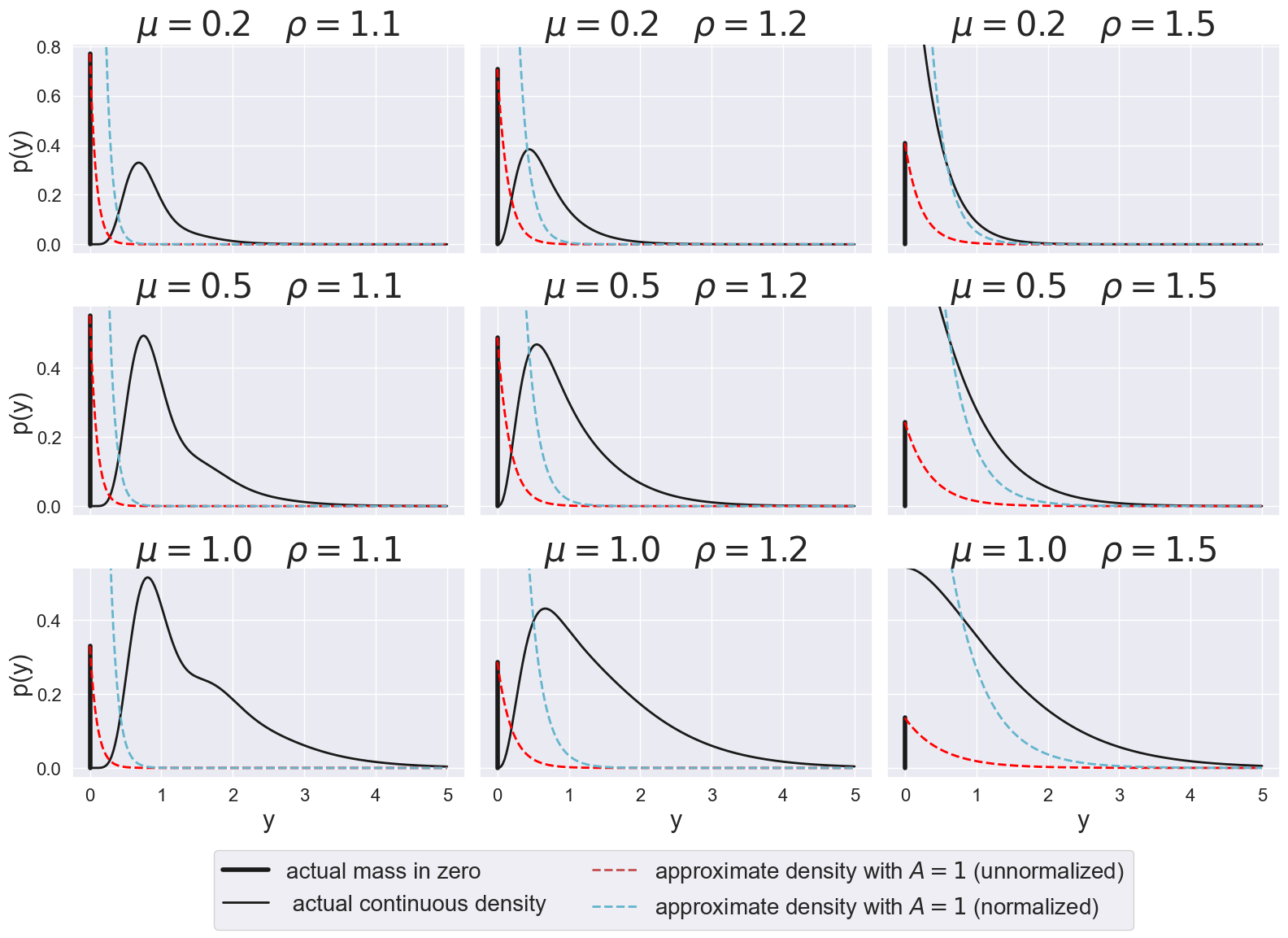
Figure 8: In this plot, $\phi=1$. In black, the Tweedie likelihood; the unnormalized density and its normalized version are the dashed lines in red and cyan respectively. The regularizing factor in the unnormalized density makes the tails shorter.

However, the resulting loss is no longer bimodal, as shown in Fig. 8, and empirical results show that having a zero-inflated behavior comes with the constraint of having short tails. For this reason its performance is not satisfactory on high quantiles, despite the use of the median demand scaling.

Appendix C Data and code availability

All data used in the experiments is publicly available.

• M5: this data set, released for the homonym competition (Makridakis et al., 2022), contains data from some Walmart stores.

• OnlineRetail: this data set contains sales records of several items in an Online store. Preprocessing was required; to extract time series from tabular sales data. These are fairly long daily series. Those in which the first sale happens toward the end of the time span, although in fact smooth, may be incorrectly classified as intermittent. For this reason, time series entirely equal to zero for the first 200 timestamps were excluded.

• Auto: short time series on automobile sales data; many of these, are not classifiable as intermittent. This data set, as well as OnlineRetail, is used by Türkmen et al. (2021).

• Carparts: similarly to RAF, monthly time series on spare parts, but for cars. This data set is provided by Hyndman (2023).

• RAF: this data set has been among the most widely used in the literature on intermittent series (e.g. Syntetos et al. (2005); Nikolopoulos et al. (2011); Snyder et al. (2012)). These monthly data represent the demand for spare parts for British Royal Air Force aircrafts.

The data sets are downloadable in the version used in the experiments by running first the file datasets.R in R and then the Python notebook datasets.ipynb. The files are located in the data folder at the GitHub page of the project, which will be released upon acceptance.

The code used for the experiments will be fully available at the GitHub link. The folder “tutorial” contains a simple usage example for our model.

The implementation of our GP models is based on GPyTorch (Gardner et al., 2018). Our contribution to public libraries is given by an implementation of the Tweedie class in the distributions module of PyTorch (Paszke et al., 2019), and the classes TweedieLikelihood and NegativeBinomialLikelihood in the likelihoods module of GPyTorch. Upon acceptance we will contribute to those packages with pull requests.

The GitHub project also contains intermittentGP class. It has methods to build, train and make predictions under the specification of the likelihood, the scaling and different traing hyperparameters, such as the number of epochs or the learning rate of the optimizer.

References

- Altay et al. (2012) Altay, N., Litteral, L.A., Rudisill, F., 2012. Effects of correlation on intermittent demand forecasting and stock control. International Journal of Production Economics 135, 275–283.
- Angelopoulos and Bates (2023) Angelopoulos, A.N., Bates, S., 2023. Conformal prediction: A gentle introduction. Found. Trends Mach. Learn. 16, 494–591.
- Babai et al. (2021) Babai, M.Z., Chen, H., Syntetos, A.A., Lengu, D., 2021. A compound-Poisson Bayesian approach for spare parts inventory forecasting. International Journal of Production Economics 232, 107954.
- Boylan and Syntetos (2021) Boylan, J.E., Syntetos, A.A., 2021. Intermittent demand forecasting: Context, methods and applications. John Wiley & Sons.
- Chapados (2014) Chapados, N., 2014. Effective bayesian modeling of groups of related count time series, in: Proc. of the 31st International Conference on Machine Learning, pp. II–1395.
- Corani et al. (2021) Corani, G., Benavoli, A., Zaffalon, M., 2021. Time Series Forecasting with Gaussian Processes Needs Priors, in: Machine Learning and Knowledge Discovery in Databases. Applied Data Science Track, Springer International Publishing, Cham. p. 103–117.
- Croston (1972) Croston, J.D., 1972. Forecasting and Stock Control for Intermittent Demands. Operational Research Quarterly (1970-1977) 23, 289.
- Dunn and Smyth (2005) Dunn, P.K., Smyth, G.K., 2005. Series evaluation of Tweedie exponential dispersion model densities. Statistics and Computing 15, 267–280.
- Gardner et al. (2018) Gardner, J., Pleiss, G., Weinberger, K.Q., Bindel, D., Wilson, A.G., 2018. GPyTorch: Blackbox Matrix-Matrix Gaussian Process Inference with GPU Acceleration, in: Advances in Neural Information Processing Systems, Curran Associates, Inc.
- Garza et al. (2022) Garza, F., Mergenthaler Canseco, M., Challú, C., Olivares, K.G., 2022. StatsForecast: Lightning fast forecasting with statistical and econometric models. PyCon Salt Lake City, Utah, US.
- Gneiting and Raftery (2007) Gneiting, T., Raftery, A.E., 2007. Strictly proper scoring rules, prediction, and estimation. Journal of the American Statistical Association 102, 359–378.
- Harvey and Fernandes (1989) Harvey, A.C., Fernandes, C., 1989. Time series models for count or qualitative observations. Journal of Business & Economic Statistics 7, 407–417.
- Hastie et al. (2009) Hastie, T., Tibshirani, R., Friedman, J.H., 2009. The Elements of Statistical Learning: Data Mining, Inference, and Prediction. 2nd ed., Springer.
- Hensman et al. (2013) Hensman, J., Fusi, N., Lawrence, N.D., 2013. Gaussian processes for big data, in: Proceedings of the Twenty-Ninth Conference on Uncertainty in Artificial Intelligence, AUAI Press. p. 282–290.
- Hensman et al. (2015) Hensman, J., Matthews, A., Ghahramani, Z., 2015. Scalable Variational Gaussian Process Classification, in: Proceedings of the Eighteenth International Conference on Artificial Intelligence and Statistics, PMLR. p. 351–360.
- Hyndman et al. (2008) Hyndman, R., Koehler, A., Ord, K., Snyder, R., 2008. Forecasting with Exponential Smoothing: The State Space Approach. Springer Series in Statistics Series, Springer Berlin / Heidelberg, Berlin, Heidelberg.
- Hyndman (2023) Hyndman, R.J., 2023. expsmooth: Data sets from ”Exponential smoothing: a state space approach” by Hyndman, Koehler, Ord and Snyder (Springer, 2008). R package version 2.4.
- Hyndman and Athanasopoulos (2021) Hyndman, R.J., Athanasopoulos, G., 2021. Forecasting: principles and practice, 3rd edition. OTexts: Melbourne, Australia.