Circulant ADMM-Net for Fast High-resolution DoA Estimation

Abstract

This paper introduces CADMM-Net and CHADMM-Net, two deep neural networks for direction of arrival estimation within the least-absolute shrinkage and selection operator (LASSO) framework. These two networks are based on a structured deep unfolding of the alternating direction method of multipliers (ADMM) algorithm through the use of circulant as well as Hermitian-circulant matrices. Along with a computational complexity of $\mathcal{O}(\mathbf{N\log(N)})$ per layer for the inference, where $\mathbf{N}$ is the length of the dictionary $\mathbf{A}$, they additionally exhibit a memory footprint of $\mathbf{N}$ and approximately half of $\mathbf{N}$ for CADMM-Net and CHADMM-Net, respectively, compared with $\mathbf{N^{2}}$ for ADMM-Net. Furthermore, these structured networks exhibit a competitive performance against ADMM-Net, LISTA, TLISTA, and THLISTA with respect to the detection rate, the angular root-mean square error, and the normalized mean squared error.

I Introduction

Fast and high-resolution direction of arrival estimation (DoA) is one key aspect required to enable advanced driver-assistance systems [1]. Automotive settings add an additional layer of complexity compared with conventional DoA estimation in that the number of snapshots typically available is very limited, with only a single snapshot being the most typical case. This renders the use of subspace-based methods such as the multiple signal classification (MUSIC) [2] and estimation of signal parameters via rotational invariant techniques (ESPRIT) [3] inadequate unless forward-backward spatial-smoothing (FBSS) [4] is employed, which reduces the array aperture in addition to constraining the geometry of the full array used since, up to a translation factor, the subarrays themselves must have an identical geometry. This precludes these subspace-based methods from being employed with the typical sparse linear arrays found in an automotive setting such as minimum redundancy arrays [5]. Maximum likelihood [6] based methods also prove impractical in this setting as they require an extensive multidimensional grid search, and becomes even more so for two dimensional arrays. Gridless methods such as atomic norm minimization (ANM) [7][8] and re-weighted atomic norm minimization (RAM) [9], despite their high-resolution, also suffer from a high-computational cost as they require $\mathcal{O}(M^{3})$ operations, where $M$ is the array size, in order to perform a projection onto the space of positive semi-definite matrices per iteration. Grid-based methods that exploit the sparse representation of the single-snapshot measurement vector $\mathbf{y}$ with respect to an overcomplete dictionary such as the least absolute shrinkage and selection operator (LASSO) [10] and sparse bayesian learning (SBL) [11] emerge as a promising contender as they can too achieve high-resolution beyond the Rayleigh limit while naturally accommodating the single snapshot setting without being restricted to ULAs. The performance of LASSO-based methods however depends heavily on the length of the dictionary used since an increase of the former will alleviate the grid mismatch effect [12]. On the other hand, typical solvers used such as the iterative shrinkage thresholding algorithm (ISTA) and the alternating direction method of moments (ADMM) require multiple iterations [13], often exceeding a hundred, to converge, with a typical computational cost per iteration of $\mathcal{O}(N^{2})$ where $N$ is the dictionary length. Thus, enhancing the performance of the sparse recovery algorithm used by increasing the dictionary length will inevitably lead to a an increase in the computational cost, effectively hindering their use in real-time automotive applications.

Deep unfolding [14] or unrolling was later on introduced to address the high-number-of-iterations aspect of these methods whereby a neural network with an architecture identical to that of the iterative method itself, such as ISTA or ADMM, is trained over a dataset with predefined statistics. Such a procedure typically results in a neural network that can compete with the iterative method being unfolded while having a depth that is considerably smaller than the number of iterations required by the method. Although the number of iterations can be reduced through deep unfolding, for an automotive setting with typically limited compute hardware, the computational cost of doing such an inference for each range-Doppler cell is still considered high. Additionally, each layer of the resulting neural network will require the storage of weight matrices whose dimension will grow with the size of the dictionary used. For instance, Learned-ISTA (LISTA) [14], a deep unrolled network based on ISTA, requires two weight matrices $\mathbf{W_{1}}\in\mathbb{C}^{N\times N}$ and $\mathbf{W_{2}}\in\mathbb{C}^{N\times M}$ to be stored for each layer. Structured deep unfolding [15] was later-on introduced to bring the memory footprint down by restricting the learnable matrices during the training phase to the class of structured ones. For instance, Toeplitz-LISTA [15], or TLISTA, restricts $\mathbf{W_{1}}$ to the set of Toeplitz matrices, thereby reducing the memory footprint from $N^{2}$ to $2N-1$ for $\mathbf{W_{1}}$. The use of Toeplitz matrices also has the added benefit of bringing down the computational cost associated with the multiplication with $\mathbf{W_{1}}$ from $N^{2}$ to $4N\log(2N)$, with the total cost per layer for TLISTA being $MN+4N\log(2N)$ compared to $N^{2}+MN$ for LISTA. Another compact versions of LISTA is Trainable-ISTA (TISTA) [16]. Although TISTA significantly reduces the total number of learnable parameters from $(N^{2}+M)T$ to $T$, where $T$ is the number of layers, this unfolded architecture was derived under the restrictive assumption of a Gaussian dictionary, which does not hold for frequency estimation wherein the dictionary typically consists of a row sub-sampled discrete Fourier transform basis.

We consider here a similar approach to TLISTA in order to build Circulant ADMM-Net and Circulant-Hermitian ADMM-Net, respectively abbreviated as CADMM-Net and CHADMM-Net. These two deep neural networks exploit the closure of the set of circulant matrices and circulant as well as Hermitian matrices to build structured versions of ADMM-Net, a deep unfolded network based on ADMM. CADMM-Net and CHADMM-Net require learnable vectors with $N$ and $\left\lfloor{N/2}\right\rfloor+1$ parameters per layer, respectively, compared with $N^{2}$ for ADMM-Net. Through the use of fast Fourier transforms (FFT) and inverse fast Fourier transforms (IFFT), the computational cost per layer for both CADMM-Net and CHADMM-Net reduces to $2N\log(N)$ compared to $N^{2}$ for ADMM-Net. The main contributions of this work can be summarized as follows:

• We introduce two neural networks termed CADMM-Net and CHADMM-Net that are based on a structured deep unfolding of ADMM that exploit circulant and Hermitian-circulant matrices, respectively.

• We study the performance of these two networks against both ISTA, ADMM as well as LISTA, ADMM-Net, TLISTA and THLISTA for both the uniform linear array (ULA) and sparse linear array (SLA) settings. The introduced models outperform the other deep-unfolded architectures with respect to the detection rate, the angular root mean squared error (RMSE), and the normalized mean squared error of the reconstructed vectors (NMSE). while having a lower per-layer computational complexity and memory footprint.

The rest of the paper is structured as follows. The signal model along with the network architecture for CADMM-Net and CHADMM-Net are presented in Section II. Section III covers in detail the experimental setup as well as the training setup used to benchmark the performance of CADMM-Net and CHADMM-Net. Section IV presents the results obtained with respect to the detection rate, the RMSE, and the NMSE as compared against ADMM-Net, LISTA, TLISTA, THLISTA as well as ADMM and ISTA. Section V provides a conclusion for this paper.

Notation: $\mathbb{C}$, $\mathbb{R}^{+}$, $\mathbb{N}$ denotes the set of complex, real positive and natural numbers, respectively. Matrices are denoted by bold uppercase letters ($\mathbf{A}$), and vectors by bold lowercase letters ($\mathbf{a}$). $|z|$ and $\textrm{arg}(z)$ denote the magnitude and argument, respectively, of the complex number $z$. $(.)^{H}$ denotes the Hermitian transpose, $(.)^{\dagger}$ denotes the pseudo-inverse, and $\overline{(.)}$ denotes the complex conjugate. $\textrm{diag}(\mathbf{v})$ denotes the diagonal matrix obtained by placing the elements of $\mathbf{v}$ in a diagonal fashion in the square null matrix. $\mathcal{CN}(\mathbf{0},\sigma^{2}\mathbf{I})$ denotes the multivariate complex normal distribution with mean $\mathbf{0}$ and covariance matrix $\sigma^{2}\mathbf{I}$. $\mathbf{X}(:,k)$ denotes the $k$-th column of $\mathbf{X}$. $\mathbf{x}\odot\mathbf{y}$ denotes the element-wise product of $\mathbf{x}$ and $\mathbf{y}$. $\mathbf{x}\ast\mathbf{y}$ denotes the discrete convolution of $\mathbf{x}$ with $\mathbf{y}$. $\mathbf{x}^{-1}$ denotes the element-wise inversion of $\mathbf{x}$, and $\mathbf{1}_{N}$ denotes the ones vector of size $N$. $\left\lfloor{x}\right\rfloor$ denotes the largest integer less than or equal to $x$.

II Network Architecture

II-A Signal Model

We consider $K$ targets impinging on a linear array with elements positioned at coordinates $d_{1},d_{2},\ldots,d_{M}$ with respect to some arbitrary origin. The resulting single-snapshot signal model can be formulated as

$$\mathbf{y}=\sum_{k=1}^{K}c_{k}\mathbf{a}(\theta^{*}_{k})+\mathbf{n}$$ (1)

where $c_{k}\in\mathbb{C}$ is the complex amplitude of the $k$-th target, $\mathbf{n}\sim\mathcal{CN}(\mathbf{0},\sigma^{2}\mathbf{I})$ is complex Gaussian additive noise, and $\mathbf{a}(\theta^{*}_{k})\in\mathbb{C}^{M\times 1}$ is the steering vector defined as

$$\mathbf{a}(\theta^{*}_{k})(m)=\exp(-j2\pi\frac{d_{m}}{\lambda}\sin(\theta^{*}_{k})),$$ (2)

for $m=1,2,\ldots,M$ . We furthermore assume that the array elements are positioned at integer multiples of a given wavelength unit, i.e. $d_{m}=l_{m}\gamma\lambda$, where $\gamma\in\mathbb{R}^{+}$ and $l_{m}\in\mathbb{N}$. The $k$-th frequency $f^{*}_{k}$ associated with $\theta^{*}_{k}$ is then defined as $f^{*}_{k}=-\gamma\sin(\theta^{*}_{k})$. With this configuration, we can express the steering vector as $\mathbf{a}(\theta^{*}_{k})(m)=\exp(j2\pi f^{*}_{k}l_{m})$, and we see that for $\theta_{k}^{*}\in[-\frac{\pi}{2},\frac{\pi}{2}]$, we will have $f_{k}^{*}\in[-\gamma,\gamma]$. Thus, in order to avoid aliasing of the frequencies corresponding to the angles, we must naturally have $\gamma<1/2$.

II-B LASSO Formulation

In the LASSO [10] context, given the measurement vector $\mathbf{y}$, recovering the frequencies $f^{*}_{k}$ essentially amounts to solving the following optimization problem [10]

$$\min_{\mathbf{x}}\dfrac{1}{2}||\mathbf{y}-\mathbf{A}\mathbf{x}||_{2}^{2}+\lambda||\mathbf{x}||_{1}$$ (3)

where $\lambda\in\mathbb{R}^{+}$ is a hyperparameter that balances the data consistency term with the sparsity penalty, and $\mathbf{A}\in\mathbb{C}^{M\times N}$ is the overcomplete dictionary, with $N\gg M$, defined as $\mathbf{A}(m,n)=\exp(j2\pi f_{n}l_{m})$ over the frequency grid points $f_{n}$ for $n=1,2,\ldots,N$. Estimates of the true frequencies $f^{*}_{k}$ can then be recovered from the support of the solution $\hat{\mathbf{x}}$ to (3).

II-C ISTA, LISTA, TLISTA and THLISTA

The ISTA formulation for solving (3) is given by the fixed-point iteration

$$\mathbf{x}^{(t)}=S_{\kappa_{1}}((\mathbf{I}-\mu\mathbf{A}^{H}\mathbf{A})\,\mathbf{x}^{(t-1)}+\mu\mathbf{A}^{H}\mathbf{y}),$$ (4)

with an initial value $\mathbf{x}^{(0)}$ (typically the zero vector) and a step size defined as $\mu=1/\sigma_{max}(\mathbf{A})^{2}$, where $\sigma_{max}(\mathbf{A})$ is the largest singular value of $\mathbf{A}$. Here, the soft-thresholding operator is defined by $S_{\kappa_{1}}(z)\triangleq e^{j\arg(z)}\max\bigl{(}|z|-\kappa_{1},0\bigr{)}$ with the threshold $\kappa_{1}=\mu\tau$.

In LISTA, the iterative scheme in (4) is replaced by a neural network whose $t$-th layer follows

$$\mathbf{x}^{(t)}=S_{\beta^{(t)}}(\mathbf{W}^{(t)}_{1}\,\mathbf{x}^{(t-1)}+\mathbf{W}^{(t)}_{2}\,\mathbf{y}),$$ (5)

where the parameters $(\mathbf{W}^{(t)}_{1},\mathbf{W}^{(t)}_{2},\beta^{(t)})$ are learned. A single LISTA layer entails a parameter count of $N^{2}+MN+1$ and a computational complexity of $N^{2}+MN$.

TLISTA [15] takes advantage of the fact that when the frequencies $f_{n}$ are uniformly spaced (i.e., $f_{n}=f_{1}+(n-1)\Delta f$), the matrix $\mathbf{A}^{H}\mathbf{A}$ becomes Toeplitz, as is $(\mathbf{I}-\mu\mathbf{A}^{H}\mathbf{A})$. In this case, the learnable matrix $\mathbf{W}^{(t)}_{1}$ is constrained to be Toeplitz and can be fully described by a single vector $\mathbf{w}^{(t)}_{1}\in\mathbb{C}^{2N-1}$. This reduces both the number of parameters and the computational cost per layer to $2N-1+MN$ and $MN+4N\log(2N)$, respectively. Moreover, by imposing an additional Hermitian constraint on $\mathbf{W}^{(t)}_{1}$, one obtains Toeplitz-Hermitian LISTA (THLISTA).

II-D ADMM and ADMM-Net

Along with coordinate-descent, ADMM [17] is widely employed to solve the optimization problem in (3). A significant benefit of ADMM over ISTA is that it typically exhibits a higher convergence rate, often requiring far fewer iterations [13]. The LASSO problem in (3) is typically reformulated into the following equivalent constrained formulation, making it well-suited for ADMM,

$$\min_{\mathbf{x},\mathbf{z}}\frac{1}{2}\|\mathbf{y}-\mathbf{A}\mathbf{x}\|_{2}^{2}+\lambda\|\mathbf{z}\|_{1}$$ (6)

$$\text{subject to: }\mathbf{x}=\mathbf{z}.$$

The augmented Lagrangian $L_{\rho}(\mathbf{x},\mathbf{z},\mathbf{w})$ of the above problem is then expressed as

$$L_{\rho}(\mathbf{x},\mathbf{z},\mathbf{v})=\frac{1}{2}\|\mathbf{y}-\mathbf{A}\mathbf{x}\|_{2}^{2}+\lambda\|\mathbf{z}\|_{1}-\frac{\rho}{2}\||\mathbf{v}\|_{2}^{2}+$$

$$\frac{\rho}{2}\||\mathbf{x}-\mathbf{z}+\mathbf{v}\|_{2}^{2},$$ (7)

where $\rho\in\mathbb{R}^{+}$ is a hyperparameter, $\mathbf{x}$, $\mathbf{z}$ are the so-called primal variables, and $\mathbf{v}$ is the dual variable. ADMM operates by alternating between gradient descent for $\mathbf{x}$ and $\mathbf{z}$ and gradient ascent on $\mathbf{v}$

$$\mathbf{x}^{(t)} =\underset{\mathbf{x}}{\textrm{argmin}}~L_{\rho}(\mathbf{x},\mathbf{z}^{(t-1)},\mathbf{v}^{(t-1)})$$ (8)

$$\mathbf{z}^{(t)} =\underset{\mathbf{z}}{\textrm{argmin}}~L_{\rho}(\mathbf{x}^{(t)},\mathbf{z},\mathbf{v}^{(t-1)})$$ (9)

$$\mathbf{v}^{(t)} =\mathbf{v}^{(t-1)}+\mathbf{x}^{(t)}-\mathbf{z}^{(t)}$$ (10)

which reduces to the following system

$$\mathbf{x}^{(t)}=(\mathbf{A}^{H}\mathbf{A}+\rho\mathbf{I})^{-1}\big{(}\mathbf{A}^{H}\mathbf{y}+\rho(\mathbf{z}^{(t-1)}-\mathbf{v}^{(t-1)})\big{)}$$ (11)

$$\mathbf{z}^{(t)}=S_{\kappa_{2}}(\mathbf{x}^{(t)}+\mathbf{v}^{(t-1)})$$ (12)

$$\mathbf{v}^{(t)}=\mathbf{x}^{(t)}+\mathbf{v}^{(t-1)}-\mathbf{z}^{(t)},$$ (13)

where $\kappa_{2}=\rho\lambda$, and a typical initialization with $\mathbf{0}$ for $\mathbf{x}^{(0)}$, $\mathbf{z}^{(0)}$, and $\mathbf{v}^{(0)}$. In order to derive the input-output relationships governing ADMM-Net and its structured variants, we will first recast the system above into an equivalent compact form. Replacing (12) in (13), we obtain

$$\mathbf{v}^{(t)}=\mathbf{x}^{(t)}+\mathbf{v}^{(t-1)}-S_{\kappa_{2}}(\mathbf{x}^{(t)}+\mathbf{v}^{(t-1)}).$$ (14)

Plugging (12) and (14) at step $(t-1)$ into (11), we get

$$\mathbf{x}^{(t)} =(\mathbf{A}^{H}\mathbf{A}+\rho\mathbf{I})^{-1}\big{(}\mathbf{A}^{H}\mathbf{y}+\rho(2S_{\kappa_{2}}(\mathbf{x}^{(t-1)}+\mathbf{v}^{(t-2)})$$

$$-\mathbf{x}^{(t-1)}-\mathbf{v}^{(t-2)})\big{)}.$$ (15)

Adding (14) at step $(t-1)$ to (15), defining the auxiliary variable $\mathbf{u}^{(t)}=\mathbf{x}^{(t)}+\mathbf{v}^{(t-1)}$, and setting $\mathbf{y_{F}}=\mathbf{A}^{H}\mathbf{y}$, we obtain

$$\mathbf{u}^{(t)} =(\mathbf{A}^{H}\mathbf{A}+\rho\mathbf{I})^{-1}(\mathbf{y_{F}}+\rho(2S_{\kappa_{2}}(\mathbf{u}^{(t-1)})$$

$$-\mathbf{u}^{(t-1)}))+\mathbf{u}^{(t-1)}-S_{\kappa_{2}}(\mathbf{u}^{(t-1)}).$$ (16)

After a large enough number of iterations $T$, we have $\mathbf{u}^{(T)}\approx\mathbf{u}^{(T-1)}$, along with this resulting approximation

$$\mathbf{x}^{(T)} =\mathbf{u}^{(T)}-\mathbf{v}^{(T-1)}=\mathbf{u}^{(T)}-\mathbf{u}^{(T-1)}+S_{\kappa_{2}}(\mathbf{u}^{(T)})$$

$$\approx S_{\kappa_{2}}(\mathbf{u}^{(T)}).$$ (17)

The compact approximate version of ADMM, summarized in Algorithm 1, serves as the basis for ADMM-Net and its structured variants as it allows us to recover $\mathbf{x}^{(T)}$ directly from $\mathbf{u}^{(T)}$ without the need to have $\mathbf{u}^{(T-1)}$ stored in memory.

Input: $\rho>0$, $\mathbf{u^{0}}\in\mathbb{C}^{N\times 1}$, $\mathbf{y}\in\mathbb{C}^{M\times 1}$, $\mathbf{A}\in\mathbb{C}^{M\times N}$, $T$;

$\mathbf{y_{F}}=\mathbf{A}^{H}\mathbf{y}$;

$\mathbf{Q}=(\mathbf{A}^{H}\mathbf{A}+\rho\mathbf{I})^{-1}$;

for $t:=1$ to $T$ do

    $\mathbf{u}^{(t)}=\mathbf{Q}\big{(}\mathbf{y_{F}}+\rho^{(t)}(2S_{\beta^{(t)}}(\mathbf{u}^{(t-1)})-\mathbf{u}^{(t-1)})\big{)}+\mathbf{u}^{(t-1)}-S_{\beta^{(t)}}(\mathbf{u}^{(t-1)})$ ;

   

end for

Output: $\mathbf{x}^{(T)}=S_{\kappa_{2}}(\mathbf{u}^{(T)})$;

Algorithm 1 Compact Approximate ADMM

The input-output relationship of the $t$-th layer of ADMM-Net is then given by

$$\mathbf{u}^{(t)} =(\mathbf{W}^{(t)}+\rho^{(t)}\mathbf{I})^{\dagger}\big{(}\mathbf{y_{F}}+\rho^{(t)}(2S_{\beta^{(t)}}(\mathbf{u}^{(t-1)})$$

$$-\mathbf{u}^{(t-1)})\big{)}+\mathbf{u}^{(t-1)}-S_{\beta^{(t)}}(\mathbf{u}^{(t-1)}),$$ (18)

along with only a learnable soft-thresholding operation performed on the output layer

$$\mathbf{x}^{(T)}=S_{\beta^{(T+1)}}(\mathbf{u}^{(T)}).$$ (19)

The learnable parameters of the $t$-th layer for ADMM-Net are thus $(\mathbf{W}^{(t)},\beta^{(t)},\rho^{(t)})$, with a parameter count of $N^{2}+2$ per layer, and a computational cost of $N^{3}+N^{2}$ operations during the training stage, and $N^{2}$ for the inference stage.

II-E CADMM-Net and CHADMM-Net

Although ADMM-Net is more efficient with respect to the parameter count compared to LISTA, it is still considerably higher than TLISTA, in addition to its high computational cost. Furthermore, the structured approach employed in going from LISTA to TLISTA does not hold for ADMM-Net, since even though $\mathbf{A}^{H}\mathbf{A}+\rho\mathbf{I}$ is Toeplitz, its inverse won’t necessarily be. We thus rely on the following proposition to build CADMM-Net and CHADMM-Net.

Proposition: Assume the extension $0<\gamma\leq 1/2$, along with a uniform frequency grid, i.e. $f_{n}=-\gamma+2\gamma(n-1)/{N}$, for $n=1,2,\ldots,N$ and $k_{M}<N-1$. Then $(\mathbf{A}^{H}\mathbf{A}+\rho\mathbf{I})^{-1}$ is circulant if and only if $\gamma=1/2$.

Proof: We will make use of the following definition for circulant matrices: $\mathbf{C}\in\mathbb{C}^{N\times N}$ is circulant if $\mathbf{C}$ is Toeplitz, i.e. $\mathbf{C}(n,p)=\mathbf{C}(n-p)$, and $\mathbf{C}(n,p)=\mathbf{C}(n-p+N)$ for $n-p<0$. For the reverse implication, with the definition $\mathbf{B}=\mathbf{A}^{H}\mathbf{A}$, we have

$$\mathbf{B}(n,p) =\sum_{m=1}^{M}\exp(j2\pi(f_{p}-f_{n})l_{m})$$

$$=\sum_{m=1}^{M}\exp(j4\pi\gamma\frac{(p-n)}{N}l_{m})$$

$$=\sum_{m=1}^{M}\exp(j2\pi\frac{(p-n)}{N}l_{m})=\mathbf{B}(n-p).$$ (20)

Thus a uniformity constraint on the grid enforces a Toeplitz constraint on $\mathbf{B}$. We additionally have

$$\mathbf{B}(n-p+N) =\sum_{m=1}^{M}\exp(j2\pi l_{m})\exp(j2\pi\frac{(p-n)}{N}l_{m})$$

$$=\sum_{m=1}^{M}\exp(j2\pi\frac{(p-n)}{N}l_{m})=\mathbf{B}(n-p).$$ (21)

Thus $\mathbf{B}$ is circulant. Using the closure under addition and inversion of circulants concludes the proof for the reverse. For the forward implication, assume that $(\mathbf{A}^{H}\mathbf{A}+\rho\mathbf{I})^{-1}$ is circulant and $\gamma\neq 1/2$, we then have that $\mathbf{B}=\mathbf{A}^{H}\mathbf{A}$ is also circulant from the aforementioned properties of circulants. Setting $s=p-n$, we then have $\mathbf{B}(s+N)-\mathbf{B}(s)=0$, for $s=1,2,\ldots,N-1$, or equivalently

$$\sum_{m=1}^{M}(1-\exp(j4\pi\gamma l_{m}))\exp(j4\pi\gamma\frac{s}{N}l_{m})=0.$$ (22)

Defining $\beta_{s}=\exp(j4\pi\gamma s/N)$ and $\alpha=\exp(j4\pi\gamma)$, we then have

$$\sum_{m=1}^{M}(1-\alpha^{l_{m}})\beta_{s}^{l_{m}}=0,$$ (23)

for $s=1,2,\ldots,N-1$. Furthermore, with $\gamma\neq 1/2$, we have $(1-\alpha^{l_{m}})\neq 0$ for $m=1,2,\ldots M$. Additionally, since $0<\gamma<1/2$, the $N-1$ roots $\beta_{1},\beta_{2},\ldots,\beta_{N-1}$ in (23) are distinct, but the polynomial $P(z)=\sum_{m=1}^{M}(1-\alpha^{l_{m}})z^{l_{m}}$ with degree $k_{M}<N-1$ can have at most $N-2$ distinct roots. $\blacksquare$

It is worth mentionning that with the requirement of a uniform grid only, $(\mathbf{A}^{H}\mathbf{A}+\rho\mathbf{I})^{-1}$ will in general be a centro-Hermitian [18] matrix that exhibits a conjugate symmetry with respect to its center. Similarly to circulants, such matrices are also closed under addition, multiplication and inversion and can be charachterized by approximately $\lfloor{N^{2}/4\rfloor}$ elements. As mentioned in II-A, in order to guarantee the non-aliasing of the frequencies corresponding to the angles of arrival, we must have $0<\gamma<1/2$. For the specific case of $\gamma=1/2$, the two angles $\theta_{1}=-\pi/2$ and $\theta_{2}=\pi/2$ would be indistinguishable as they would both map to the same frequency $f=-1/2$. This inconvenience may be alleviated by the fact that the radiation pattern for the antennas, very often planar, employed in automotive arrays rarely cover the full field of view from $-\pi/2$ to $\pi/2$. We will thus henceforth assume a uniform frequency grid and set $\gamma=1/2$. Using the eigendecomposition of circulant matrices, we can then write

$$(\mathbf{A}^{H}\mathbf{A}+\rho\mathbf{I})^{-1} =(\mathbf{F}^{-1}\textrm{diag}(\mathbf{F}\mathbf{b})\mathbf{F}+\rho\mathbf{F}^{-1}\mathbf{F})^{-1}$$

$$=(\mathbf{F}^{-1}(\textrm{diag}(\mathbf{F}\mathbf{b})+\rho\mathbf{I})\mathbf{F})^{-1}$$

$$=\mathbf{F}^{-1}(\textrm{diag}(\mathbf{F}\mathbf{b})+\rho\mathbf{I})^{-1}\mathbf{F}$$ (24)

where $\mathbf{F}$ and $\mathbf{F}^{-1}$ are the discrete Fourier transform (DFT) and inverse discrete Fourier transform (IDFT) matrices, respectively, and $\mathbf{b}$ is the first column of $\mathbf{B}=\mathbf{A}^{H}\mathbf{A}$. We can incorporate this change to the compact version of ADMM to yield the fast version described in Algorithm 2. Under the previous assumptions, the computational complexity of ADMM therefore reduces from $N^{2}$ per iteration to $2N\textrm{log}(N)$. Additionally, the product $\mathbf{y_{F}}=\mathbf{A}^{H}\mathbf{y}$ reduces to the evaluation of the $N$-point DFT of $\mathbf{y}$.

Input: $\rho>0$, $\mathbf{u^{0}}\in\mathbb{C}^{N\times 1}$, $\mathbf{y}\in\mathbb{C}^{M\times 1}$, $\mathbf{A}\in\mathbb{C}^{M\times N}$, $T$;

$\mathbf{y_{F}}=\mathbf{A}^{H}\mathbf{y}$;

$\mathbf{B}=\mathbf{A}^{H}\mathbf{A}$;   $\mathbf{b}=\mathbf{B}(:,1)$;

$\mathbf{q}=(\mathbf{F}\mathbf{b}+\rho\mathbf{1}_{N})^{-1}$;

for $t:=1$ to $T$ do

    $\mathbf{u}^{(t)}=\mathbf{F}^{-1}\mathbf{q}\odot\mathbf{F}\big{(}\mathbf{y_{F}}+\rho^{(t)}(2S_{\beta^{(t)}}(\mathbf{u}^{(t-1)})-\mathbf{u}^{(t-1)})\big{)}+\mathbf{u}^{(t-1)}-S_{\beta^{(t)}}(\mathbf{u}^{(t-1)})$;

   

end for

Output: $\mathbf{x}^{(T)}=S_{\kappa_{2}}(\mathbf{u}^{(T)})$;

Algorithm 2 Fast Compact Approximate ADMM

The input-output relationship of the $t$-th layer of CADMM-Net can then be stated as

$$\mathbf{u}^{(t)} =\mathbf{F}^{-1}(\mathbf{w}^{(t)}+\rho^{(t)}\mathbf{1}_{N})^{-1}\odot\mathbf{F}\big{(}\mathbf{y_{F}}+\rho^{(t)}(2S_{\beta^{(t)}}(\mathbf{u}^{(t-1)})$$

$$-\mathbf{u}^{(t-1)})\big{)}+\mathbf{u}^{(t-1)}-S_{\beta^{(t)}}(\mathbf{u}^{(t-1)}),$$ (25)

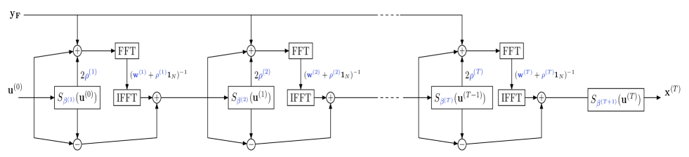
Figure 1: CADMM-Net network with $T$ layers. The learnable parameters are highlighted in blue.

TABLE I: Summary of CADMM-Net and CHADMM-Net characteristics

	ADMM-Net	CADMM-Net	CHADMM-Net
Input-output relationship	$\mathbf{u}^{(t+1)}=\big{(}\mathbf{W}^{(t)}+\rho^{(t)}\mathbf{I}\big{)}^{-1}R_{1}^{(t)}(\mathbf{u}^{(t)})$ $+R_{2}^{(t)}(\mathbf{u}^{(t)})$	$\mathbf{u}^{(t)}=\mathbf{F}^{-1}(\mathbf{w}^{(t)}+\rho^{(t)}\mathbf{1}_{N})^{-1}\odot\mathbf{F}\big{(}\mathbf{y_{F}}$ $+\rho^{(t)}R_{1}^{(t)}(\mathbf{u}^{(t-1)})\big{)}+R_{2}^{(t)}(\mathbf{u}^{(t-1)})$	$\mathbf{u}^{(t)}=\mathbf{F}^{-1}(\mathbf{F}\mathbf{w}^{(t)}+\rho^{(t)}\mathbf{1}_{N})^{-1}\odot\mathbf{F}\big{(}\mathbf{y_{F}}$ $+\rho^{(t)}R_{1}^{(t)}(\mathbf{u}^{(t-1)})\big{)}+R_{2}^{(t)}(\mathbf{u}^{(t-1)})$
Parameter count	$N^{2}+2$	$N+2$	$\left\lfloor{N/2}\right\rfloor+3$
Computational complexity	Training: $\mathcal{O}(N^{3})$ Inference: $\mathcal{O}(N^{2})$	$\mathcal{O}(N\log(N))$	$\mathcal{O}(N\log(N))$

• $R_{1}^{(t)}(\mathbf{u}^{(t)})=2S_{\beta^{(t)}}(\mathbf{u}^{(t)})-\mathbf{u}^{(t)}$ and $R_{2}^{(t)}(\mathbf{u}^{(t)})=\mathbf{u}^{(t)}-S_{\beta^{(t)}}(\mathbf{u}^{(t)})$

where the learnable parameters are ($\mathbf{w}^{(t)},\rho^{(t)},\beta^{(t)})$. Similarly $\mathbf{x}^{(T)}$ is recovered in the last layer through a learnable thresholding operation

$$\mathbf{x}^{(T)}=S_{\beta^{(T+1)}}(\mathbf{u}^{(T)}).$$ (26)

The corresponding parameter count per layer is thus $N+2$, and the computational cost is $2N\textrm{log}(N)$ operations for both training and inference, mainly dominated by the FFT and IFFT operations. The corresponding neural nertwork architecutre of a $T$-layer CADMM-Net network is shown in Fig. 1. In addition to being circulant, $\mathbf{B}=\mathbf{A}^{H}\mathbf{A}$ is also Hermitian, and so will be $(\mathbf{A}^{H}\mathbf{A}+\rho\mathbf{I})^{-1}$ since the Hermitian and inverse operators commute. A circulant Hermitian matrix is the complex extension of the circulant symmetric matrix and is highly structured as it can be fully characterized by only $\left\lfloor{N/2}\right\rfloor+1$ complex scalars. The vector $\mathbf{c}$ parameterizing a circulant Hermtian matrix $\mathbf{C}$ has the following form,

$$\mathbf{c}=[c_{1},c_{2},\ldots,c_{\left\lfloor{N/2}\right\rfloor+1},\overline{c}_{N-\left\lfloor{N/2}\right\rfloor},\overline{c}_{N-\left\lfloor{N/2}\right\rfloor-1},\ldots,\overline{c}_{2}].$$ (27)

The input-output relationship for CHADMM-Net is then given by

$$\mathbf{u}^{(t)} =\mathbf{F}^{-1}(\mathbf{F}\mathbf{w}^{(t)}+\rho^{(t)}\mathbf{1}_{N})^{-1}\odot\mathbf{F}\big{(}\mathbf{y_{F}}+\rho^{(t)}($$

$$2S_{\beta^{(t)}}(\mathbf{u}^{(t-1)})-\mathbf{u}^{(t-1)})\big{)}+\mathbf{u}^{(t-1)}-S_{\beta^{(t)}}(\mathbf{u}^{(t-1)}),$$ (28)

where the learnable parameters are ($\mathbf{w}^{(t)},\rho^{(t)},\beta^{(t)})$ and $\mathbf{w}^{(t)}\in\mathbb{C}^{N\times 1}$ satisfies the constraint

$$\mathbf{w}^{(t)}(n)=\overline{\mathbf{w}^{(t)}}(N+2-n),\quad n=\left\lfloor{N/2}\right\rfloor+2,\ldots,N.$$ (29)

During the training phase of CHADMM-Net, the constraint in (29) is applied immediately after $\mathbf{w}^{(t)}$ is updated through gradient descent. Table I provides a summary of the main characteristics of ADMM-Net along with its structured variants presented so far.

III Experimental Setup

III-A Datasets

For the training setup of CADMM-Net and CHADMM-Net, we fix the dictionary size to $N=256$ and set $\gamma=1/2$. Experiments are conducted in both ULA and SLA scenarios using an array with $M=30$ elements. In the SLA case, $30$ elements are randomly subsampled from a ULA that spans a total aperture of $60\lambda/2$. For each setting, a training set of $10^{5}$ measurement vectors and a validation set of $2\times 10^{4}$ measurement vectors are generated together with their corresponding ground truth vectors. The number of targets $K$ is selected uniformly at random from between $1$ and $8$. Afterwards, $K$ frequencies $f_{k}^{*}$, for $k=1,2,\ldots,K$, are drawn from the interval $[-1/2,1/2[$ while ensuring that the difference between any two frequencies is at least $1/M$ [19]. Subsequently, each frequency $f_{k}^{*}$ is mapped to its nearest grid point $f_{k}$. For every $f_{k}$, an amplitude $x_{k}$ is generated with $|x_{k}|\sim\mathcal{U}(0,1)$ and $\textrm{arg}(x_{k})\sim\mathcal{U}(0,2\pi)$, thereby constructing the ground truth vector $\mathbf{x}$. Finally, the signal-to-noise ratio (SNR) is fixed at 15 dB, and the measurement vector $\mathbf{y}$ corresponding to $\mathbf{x}$ is produced as

$$\mathbf{y}=\sum_{k=1}^{K}x_{k}\mathbf{a}(f^{*}_{k})+\mathbf{n}$$ (30)

with $\mathbf{n}\sim\mathcal{CN}(\mathbf{0},\sigma^{2}\mathbf{I})$, where

$$\sigma^{2}=10^{-\frac{\textrm{SNR}}{10}}\Bigl{\|}\sum_{k=1}^{K}x_{k}\mathbf{a}(f^{*}_{k})\Bigr{\|}_{2}^{2}.$$

For the performance evaluation in terms of the NMSE, RMSE, and detection rate, we decrease the minimum frequency separation constraint from $1/M$ to $1/(3M)$ and generate a test set consisting of $10^{3}$ measurement vectors, together with their corresponding ground truth, for each SNR level ranging from 0 dB to 35 dB in increments of 5 dB.

TABLE II: Constraints and initialization of the learnable weights

	ADMM-Net	CADMM-Net	CHADMM-Net	LISTA	TLISTA
Weights	$\mathbf{W}^{(t)}$	$\mathbf{w}^{(t)}$	$\mathbf{w}^{(t)}$	$(\mathbf{W}_{1}^{(t)},\mathbf{W}_{2}^{(t)})$	$(\mathbf{W}_{1}^{(t)},\mathbf{W}_{2}^{(t)})$
Constraint	$\mathbf{W}^{(t)}\in\mathbb{C}^{N\times N}$	$\mathbf{w}^{(t)}\in\mathbb{C}^{N\times 1}$	$\mathbf{w}^{(t)}(n)=\overline{\mathbf{w}^{(t)}}(N+2-n)$ $n=\left\lfloor{N/2}\right\rfloor+2,\ldots,N$	$\mathbf{W}_{1}^{(t)},\mathbf{W}_{2}^{(t)}\in\mathbb{C}^{N\times N}$	$\mathbf{W}_{1}^{(t)}(n,p)=\mathbf{W}_{1}^{(t)}(n-p)$ $\mathbf{W}_{2}^{(t)}\in\mathbb{C}^{N\times N}$
Initialization	$\mathbf{W}^{(t)}=\mathbf{A}^{H}\mathbf{A}$	$\mathbf{w}^{(t)}=\mathbf{F}\mathbf{b}$	$\mathbf{w}^{(t)}=\mathbf{b}$	$\mathbf{W}_{1}^{(t)}=\mathbf{A}^{H}\mathbf{A}$ $\mathbf{W}_{2}^{(t)}=\mu\mathbf{A}^{H}$	$\mathbf{W}_{1}^{(t)}=\mathbf{A}^{H}\mathbf{A}$ $\mathbf{W}_{2}^{(t)}=\mu\mathbf{A}^{H}$

III-B Training Setup

We compare CADMM-Net and CHADMM-Net against ADMM-Net, LISTA, TLISTA and THLISTA as well as a 100 iteration of ADMM and ISTA. We fix the number of layers $T$ for all the networks to $30$. For the initialization, all the weight matrices and vectors in all the layers of all the networks are initialized with their respective value in the corresponding iterative method. For instance, for CADMM-Net, $\mathbf{w}^{(t)}$ is initialized with $\mathbf{Fb}$, where $\mathbf{b}$ is the first column of $\mathbf{A}^{H}\mathbf{A}$, for all layers $t=1,2,\ldots 30$. Table II provides a summary of the initialization and constraints for the weights of the networks used. Additionally, $\beta^{(t)}$ is initalized with $10^{-1}$ for all networks and $\rho^{(t)}$ is initialized with 1 for ADMM-Net and its structured variants. We use the Adam [20] optimizer with a learning rate of $10^{-4}$ along with a batch size of 2048.

III-C Loss function

The standard NMSE loss in the way it is typically used between the output of the neural network $\mathbf{x}^{(T)}$ and the ground truth vector $\mathbf{x}$,

$$\textrm{NMSE}(\mathbf{x}^{(T)},\mathbf{x})=\frac{||\mathbf{x}^{(T)}-\mathbf{x}||_{2}^{2}}{||\mathbf{x}||^{2}},$$ (31)

is not a smooth function with respect to the support itself. For instance, let us consider a sparse ground truth vector consisting of a single non-zero component, $\mathbf{x}(n)=x_{0}\delta(f_{n}-f_{n_{0}})$. Assuming an output from the neural net of a similar form but with a shifted support, $\mathbf{x}^{(T)}(n)=x_{1}\delta(f_{n}-f_{n_{1}})$, the resulting NMSE as a function of the mismatch with respect to the frequency support, $\Delta f=|f_{n_{0}}-f_{n_{1}}|$, would assume the following form,

$$\textrm{NMSE}(\Delta f)=\begin{cases}|x_{1}-x_{0}|^{2}/|x_{0}|^{2}&\text{if }\Delta f=0\\ (|x_{1}|^{2}+|x_{0}|^{2})/|x_{0}|^{2}&\text{if }\Delta f\neq 0.\end{cases}$$ (32)

Thus, when there is a mismatch, this loss ascribes the same constant value, regardless of how large or small this mismatch can be. Therefore, before computing the loss, both $\mathbf{x}^{(T)}$ and $\mathbf{x}$ are convolved with a zero-mean Laplacian kernel $\mathbf{g}$ with a scale parameter $b>0$

$$\mathbf{g}(n)=\exp(-|n|/b),\quad n=-\left\lfloor{N/2}\right\rfloor,\ldots,\left\lfloor{N/2}\right\rfloor,$$ (33)

we afterwards use $\textrm{NMSE}(\mathbf{x}^{(T)}\ast\mathbf{g},\mathbf{x}\ast\mathbf{g})$ as the loss function. Using the same previous example of a sparse vector with a single component. Fig. 2 shows the resulting loss with this method. Naturally, the increase in sensitivity of the loss function with respect to $\Delta f$ for higher values of $b$ is simultaneuous with the risk of lower amplitude targets being submerged by the tails of the stronger ones after the convolution operation. We thus settle for $b=1/2$ as a middle ground for our loss function. It is worth mentioning that another loss function that quantifies support mismatch is the Sinkhorn distance [21]. However this loss function requires multiple iterations to converge, and thus effectively extends the depth of the network during the training phase since the full computational graph [22] needs to be stored during the forward pass. It additionaly suffers from numerical instability issue, and although there is a log-stabilized version [23], it still adds a considerable overhead for both memory and compute and proved to be too impractical to use in our experiments.

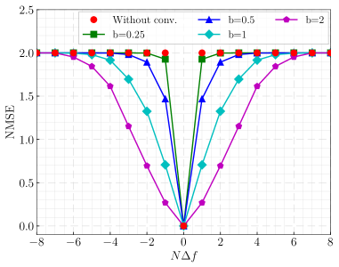
Figure 2: NMSE between a single-component sparse vector and a support-shifted version, both of which are convolved with a Laplacian kernel.

III-D Metrics

III-E Peformance Comparaison

To evaluate the performance of CADMM-Net and CHADDM-Net against the other networks, we employ the detection rate and the root mean-squared error (RMSE). First, using either a neural network or an iterative technique, we obtain an estimate $\mathbf{\hat{x}}$ of the ground-truth vector $\mathbf{x}$ corresponding to a measurement vector $\mathbf{y}$. We then perform peak detection on the amplitude spectrum to derive a new spectrum $\mathbf{\hat{x}}_{pk}$ that retains only the peak values from $|\mathbf{\hat{x}}|$. For a target in the ground-truth spectrum $|\mathbf{x}|$ that appears at a frequency bin indexed by $r$ on the uniform grid, we identify the set of indices

$$\mathcal{I}_{r}=\{\hat{r}_{1},\hat{r}_{2},\ldots,\hat{r}_{L(r)}\},$$ (34)

comprising the estimated support values from $|\mathbf{\hat{x}}|$ that satisfy

$$|r-\hat{r}_{l}|\leq\delta_{1},\qquad l=1,2,\ldots,L(r).$$ (35)

Next, from $\mathcal{I}_{r}$ we keep only those indices forming the subset $\mathcal{J}_{r}\subseteq\mathcal{I}_{r}$ where the ratio between the amplitude of the estimated spectrum and the ground-truth amplitude exceeds a predefined threshold $0<\delta_{2}\leq 1$, i.e.,

$$\dfrac{\mathbf{\hat{x}}_{pk}(j)}{|\mathbf{x}(r)|}\geq\delta_{2},\qquad j\in\mathcal{J}_{r}.$$ (36)

If $\mathcal{J}_{r}$ is non-empty, then the recovery corresponding to the target at frequency bin $r$ is deemed successful. This process is repeated for all $K$ targets present in a ground-truth vector $\mathbf{x}$. Defining the indicator function as $\mathds{1}(\phi)=1$ if $\phi\neq\emptyset$ and $0$ otherwise, the detection rate $P_{d}$ is given by

$$P_{d}=\dfrac{\sum_{k=1}^{K}\mathds{1}(\mathcal{J}_{r(k)})}{K}.$$ (37)

For each SNR level, we report the mean detection rate computed over a test set of 1000 measurement vectors. For the RMSE computation, consider the $k$-th ground-truth target located at the frequency bin $r(k)$. We first determine the index $\tilde{j}(k)$ in $\mathcal{J}_{r(k)}$ that is closest to $r(k)$:

$$\tilde{j}(k)=\operatorname*{\arg\!\min}\limits_{j\in\mathcal{J}_{r(k)}}|j-r(k)|.$$ (38)

Letting $\theta_{n}=\sin^{-1}(f_{n})/\gamma$ denote the angle corresponding to the $n$-th frequency bin, the mean squared angular error $E$ for a single test vector is calculated as

$$E=\dfrac{1}{N_{d}}\sum_{s=1}^{N_{d}}\Bigl{(}\theta_{r(k_{s})}-\theta_{\tilde{j}(k_{s})}\Bigr{)}^{2},$$ (39)

where $N_{d}=\sum_{k=1}^{K}\mathds{1}(\mathcal{J}_{q(k)})$ denotes the number of targets successfully detected. For each SNR level, we calculate the average angular error $E$ over all test vectors with at least one successful detection, and then take the square root of this average to obtain the RMSE. In our experiments, we set the parameters $(\delta_{1},\delta_{2})=(2,0.4)$. In addition, we report the performance with respect to the NMSE.

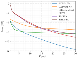
(a) Training loss.

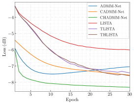
(b) Validation loss.

Figure 3: Training (a) and validation (b) losses for the SLA setting.

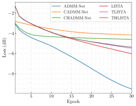
(a) Training loss.

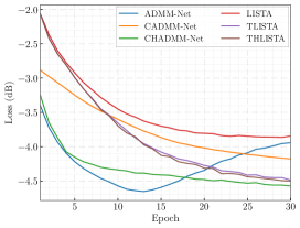
(b) Validation loss.

Figure 4: Training (a) and validation (b) losses for the ULA setting.

IV Results

IV-A Training Losses

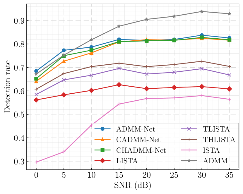
(a) Detection rate.

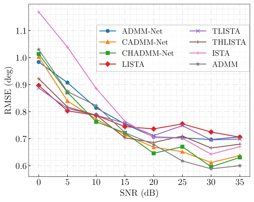
(b) RMSE.

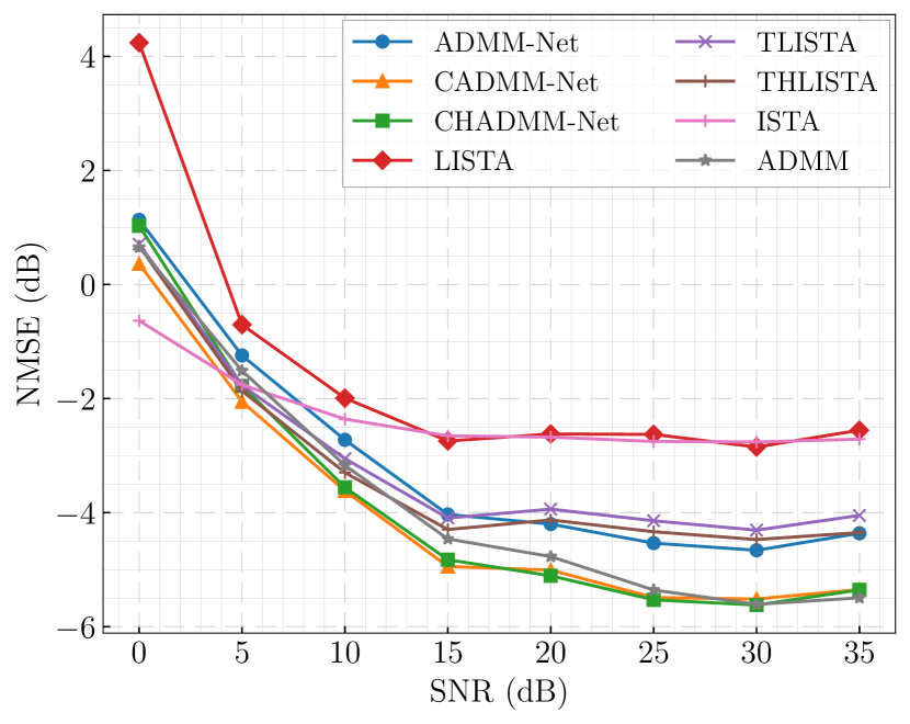
(c) NMSE.

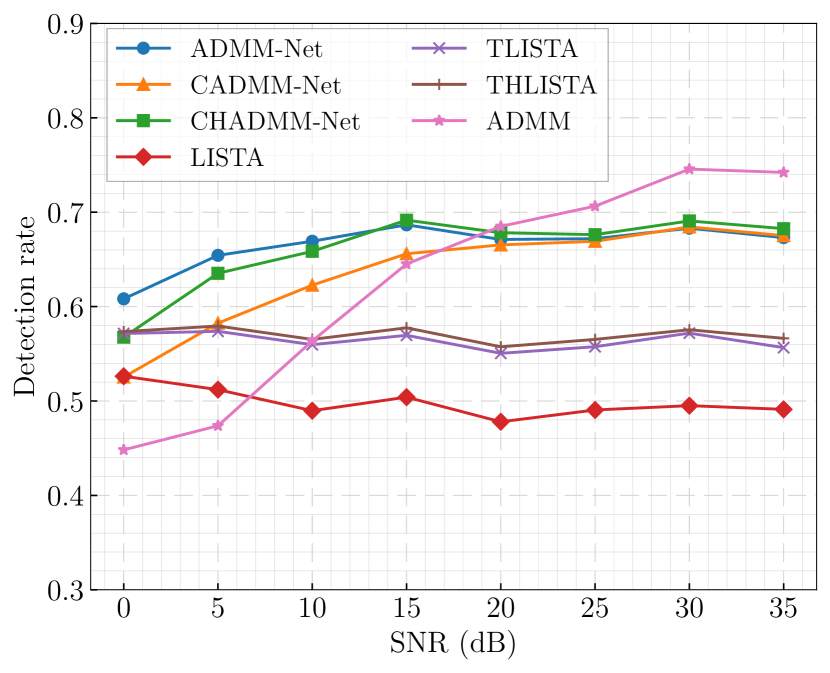
(d) Detection rate.

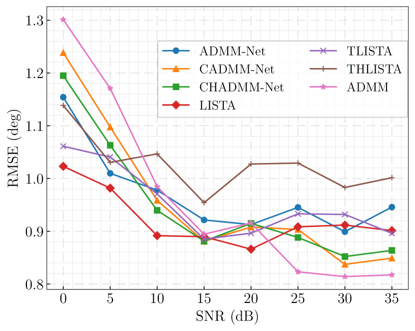
(e) RMSE.

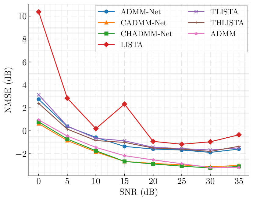
(f) NMSE.

Figure 5: Performance comparison for the 20-element SLA (top row) and ULA (bottom row) scenarios. All networks are 30-layers deep. ISTA and ADMM are set to 100 iterations.

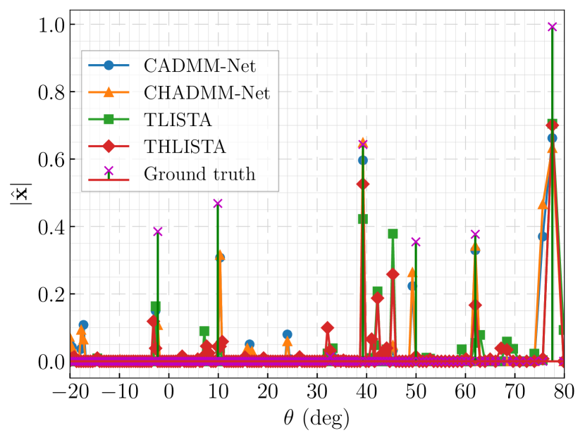
(a)

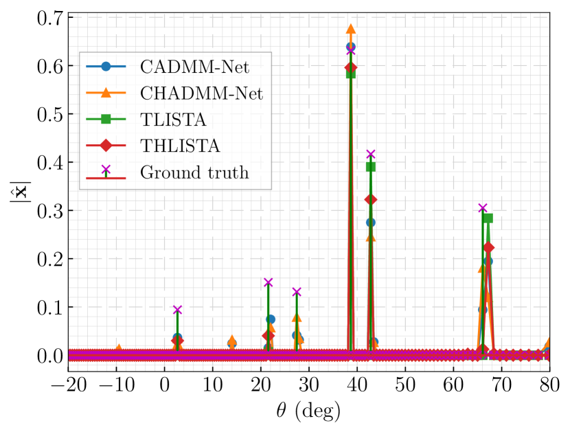
(b)

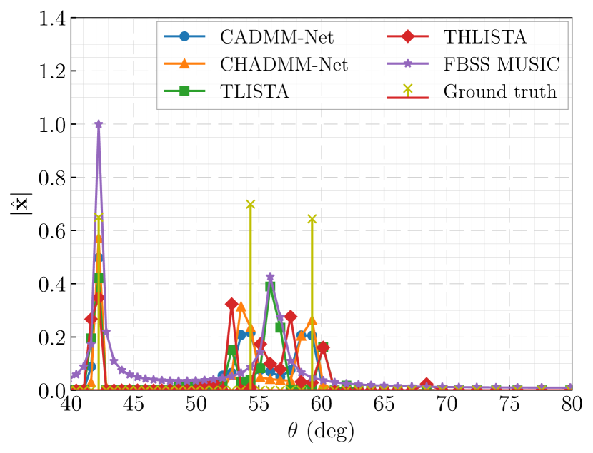
(c)

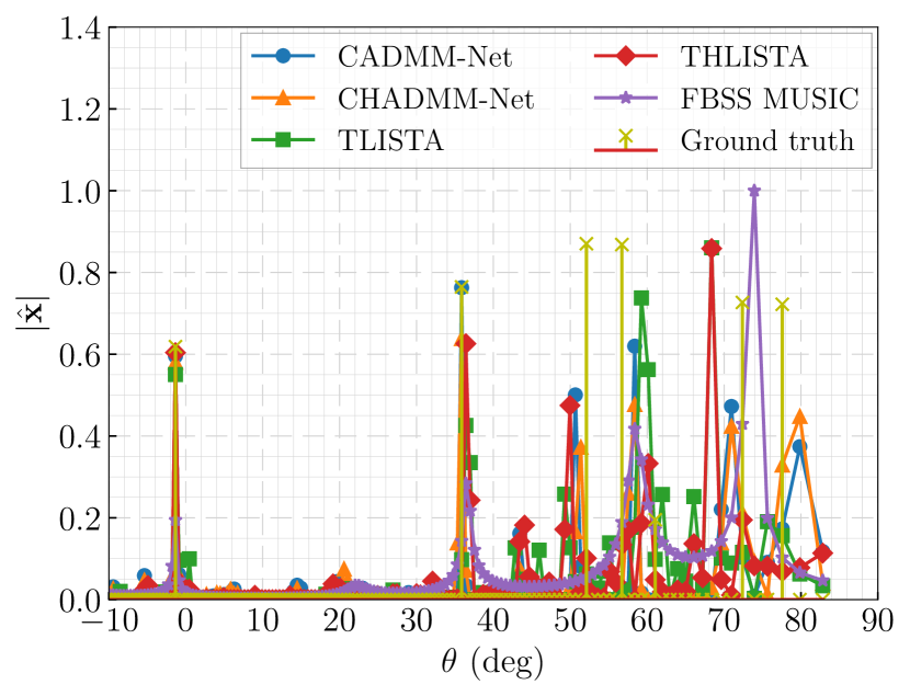
(d)

Figure 6: Sample spectrums at 10 dB SNR, top row SLA with 60$\lambda/2$ aperture and 30 elements, bottorm row ULA with 30 elements. The subarray size is set to 10 for FBSS MUSIC.

The training curves Fig. 3 and Fig. 4 indicate that the structured versions tend to learn faster than the unstructured ones. Notably, we can see from figure Fig. 3(b) that CHADMM-Net under the SLA setting has most of its validation loss decrease during the first 10 epochs only. This stands in sharp contrast with the learning behavior of ADMM-Net, which begins to overfit after the 13-th epoch. One additional observation woth noting is despite LISTA having more parameters than ADMM-Net, it does not exhibit the same overfitting pattern, which indicates that the learning behavior of deep-unfolded networks can be largely influenced by the choice of the iterative method being unfolded, as LISTA and ADMM-Net are architecturally different.

Finally, we can note that the networks are able to learn better under the SLA setting compared to the ULA one, which can in part be explained with the fact that the SLA setting, with an identical number of elements but larger aperture, is more favorable for the recovery of sparse signals with closely spaced frequencies.

IV-B Performance Comparison

Fig. 5(a) and 5(d) show the detection rate performance of the networks along with a 100 iteration of ADMM and ISTA. For the iterative methods, we report the ADMM performance only for the ULA setting as ISTA was significantly underperforming. We can note that CHADMM-Net is able to outperform all the other networks in terms of detection rate for both the SLA and ULA settings over an SNR ranging from 0 dB up to 35 dB, with an average detection rate of 80% in the high SNR region compared with an average of 70% for TLISTA and THLISTA. We can also note that both CADMM-Net and CHADMM-Net show a comparable performance against ADMM in the low SNR region for the SLA setting.

For the RMSE performance unde the SLA setting, we can see from Fig. 5(b) that CHADMM-Net and CADMM-Net outperform TLISTA and THLISTA over an SNR ranging from approxitamtely 10 dB up to 35 dB, and a comparable performance in the ULA setting for an SNR going from 5 dB up to 35 dB, as seen from Fig. 5(e). Finally, for the NMSE performance, we can note again that CHADMM-Net outpeforms all the other networks across the full SNR range from 0 dB up to 35 dB.

Fig. 6(a) shows a sample spectrum for the SLA setting at 10 dB SNR, where we can see that CHADMM-Net is able to recover the ground truth spectrum with a higher accuracy compared to the other networks. The same can be observed in the ULA setting from Fig. 6(d) in which we added a forward-backward spatially smoothed MUSIC spectrum for reference and where the true number of targets is directly provided. We can see that CHADMM-Net is able to detect all the 6 peaks present in the ground truth spectrum while having much less false positives compared to the other networks.

V Conclusion

We presented CADMM-Net and CHADMM-Net two deep-unfolded versions of ADMM that impose a circulant and Hermitian-circulant constraint on the learnable matrices so as to both considerably reduce the number of learnable parameters per layer as well as decrease the computational complexity while achieving a competitive performance compared with LISTA, ADMM-Net, TLISTA, and THLISTA as well as ISTA and ADMM with respect to the detection rate, the RMSE, and the NMSE.

References

- [1] F. Engels, P. Heidenreich, M. Wintermantel, L. Stäcker, M. Al Kadi, and A. M. Zoubir, “Automotive radar signal processing: Research directions and practical challenges,” IEEE Journal of Selected Topics in Signal Processing, vol. 15, no. 4, pp. 865–878, 2021.
- [2] W. Liao and A. Fannjiang, “Music for single-snapshot spectral estimation: Stability and super-resolution,” Applied and Computational Harmonic Analysis, vol. 40, no. 1, pp. 33–67, 2016.
- [3] R. Roy and T. Kailath, “Esprit-estimation of signal parameters via rotational invariance techniques,” IEEE Transactions on Acoustics, Speech, and Signal processing, vol. 37, no. 7, pp. 984–995, 1989.
- [4] S. U. Pillai and B. H. Kwon, “Forward/backward spatial smoothing techniques for coherent signal identification,” IEEE Transactions on Acoustics, Speech, and Signal Processing, vol. 37, no. 1, pp. 8–15, 1989.
- [5] A. Moffet, “Minimum-redundancy linear arrays,” IEEE Transactions on Antennas and Propagation, vol. 16, no. 2, pp. 172–175, 1968.
- [6] P. Stoica and K. C. Sharman, “Maximum likelihood methods for direction-of-arrival estimation,” IEEE Transactions on Acoustics, Speech, and Signal Processing, vol. 38, no. 7, pp. 1132–1143, 1990.
- [7] Z. Yang and L. Xie, “Enhancing sparsity and resolution via reweighted atomic norm minimization,” IEEE Transactions on Signal Processing, vol. 64, no. 4, pp. 995–1006, 2015.
- [8] M. Wagner, Y. Park, and P. Gerstoft, “Gridless doa estimation and root-music for non-uniform linear arrays,” IEEE Transactions on Signal Processing, vol. 69, pp. 2144–2157, 2021.
- [9] B. N. Bhaskar, G. Tang, and B. Recht, “Atomic norm denoising with applications to line spectral estimation,” IEEE Transactions on Signal Processing, vol. 61, no. 23, pp. 5987–5999, 2013.
- [10] R. Tibshirani, “Regression shrinkage and selection via the lasso,” Journal of the Royal Statistical Society Series B: Statistical Methodology, vol. 58, no. 1, pp. 267–288, 1996.
- [11] D. P. Wipf and B. D. Rao, “Sparse bayesian learning for basis selection,” IEEE Transactions on Signal processing, vol. 52, no. 8, pp. 2153–2164, 2004.
- [12] Y. Chi, L. L. Scharf, A. Pezeshki, and A. R. Calderbank, “Sensitivity to basis mismatch in compressed sensing,” IEEE Transactions on Signal Processing, vol. 59, no. 5, pp. 2182–2195, 2011.
- [13] S. Tao, D. Boley, and S. Zhang, “Convergence of common proximal methods for l1-regularized least squares,” in Twenty-Fourth International Joint Conference on Artificial Intelligence, 2015.
- [14] K. Gregor and Y. LeCun, “Learning fast approximations of sparse coding,” in Proceedings of the 27th International Conference on Machine Learning, 2010, pp. 399–406.
- [15] R. Fu, Y. Liu, T. Huang, and Y. C. Eldar, “Structured lista for multidimensional harmonic retrieval,” IEEE Transactions on Signal Processing, vol. 69, pp. 3459–3472, 2021.
- [16] D. Ito, S. Takabe, and T. Wadayama, “Trainable ista for sparse signal recovery,” IEEE Transactions on Signal Processing, vol. 67, no. 12, pp. 3113–3125, 2019.
- [17] S. Boyd, N. Parikh, E. Chu, B. Peleato, J. Eckstein et al., “Distributed optimization and statistical learning via the alternating direction method of multipliers,” Foundations and Trends® in Machine learning, vol. 3, no. 1, pp. 1–122, 2011.
- [18] A. Lee, “Centrohermitian and skew-centrohermitian matrices,” Linear Algebra and its Applications, vol. 29, pp. 205–210, 1980, special Volume Dedicated to Alson S. Householder. [Online]. Available: https://www.sciencedirect.com/science/article/pii/0024379580902414
- [19] E. Candes and C. Fernandez-Granda, “Towards a mathematical theory of super-resolution,” 2012. [Online]. Available: https://arxiv.org/abs/1203.5871
- [20] D. P. Kingma and J. Ba, “Adam: A method for stochastic optimization,” arXiv preprint arXiv:1412.6980, 2014.
- [21] M. Cuturi, “Sinkhorn distances: Lightspeed computation of optimal transport,” in Advances in Neural Information Processing Systems, C. Burges, L. Bottou, M. Welling, Z. Ghahramani, and K. Weinberger, Eds., vol. 26. Curran Associates, Inc., 2013.
- [22] “Autograd mechanics,” Pytorch Docs, 2025. [Online]. Available: https://pytorch.org/docs/stable/notes/autograd.html
- [23] G. Peyré and M. Cuturi, “Computational optimal transport,” 2020.