Foundation Inference Models for Stochastic Differential Equations: \0.15cm A Transformer-based Approach for Zero-shot Function Estimation

Abstract

Stochastic differential equations (SDEs) describe dynamical systems where deterministic flows, governed by a drift function, are superimposed with random fluctuations dictated by a diffusion function. The accurate estimation (or discovery) of these functions from data is a central problem in machine learning, with wide application across natural and social sciences alike. Yet current solutions are brittle, and typically rely on symbolic regression or Bayesian non-parametrics. In this work, we introduce FIM-SDE (Foundation Inference Model for SDEs), a transformer-based recognition model capable of performing accurate zero-shot estimation of the drift and diffusion functions of SDEs, from noisy and sparse observations on empirical processes of different dimensionalities. Leveraging concepts from amortized inference and neural operators, we train FIM-SDE in a supervised fashion, to map a large set of noisy and discretely observed SDE paths to their corresponding drift and diffusion functions. We demonstrate that one and the same (pretrained) FIM-SDE achieves robust zero-shot function estimation (i.e. without any parameter fine-tuning) across a wide range of synthetic and real-world processes, from canonical SDE systems (e.g. double-well dynamics or weakly perturbed Hopf bifurcations) to human motion recordings and oil price and wind speed fluctuations.

Our pretrained model, repository and tutorials are available online.

1 Introduction

Stochastic differential equations (SDEs) govern dynamical systems featuring deterministic flows superimposed with random fluctuations. The deterministic component of these systems are dictated by a drift function, and are used to model the slow, tractable or accessible degrees of freedom of dynamic phenomena. The random components are instead controlled by a diffusion function, and are used to represent fast or intractable degrees of freedom. Such a description, in terms of tractable versus intractable, slow versus fast, is abstract enough to be applicable across disciplines and observation scales. It was first employed to capture variations of derivative pricing in financial markets (Bachelier, 1900), and almost immediately to understand the patterns traced by particles suspended in liquids (Einstein, 1905). It was famously applied to link slow climate variability to rapid weather fluctuations (Hasselmann, 1976), and to represent the coupling with intractable environments in population genetics (Turelli, 1977). However, the central problem limiting the actual applicability of the SDE description to many complex phenomena, is the accurate determination of the drift and diffusion functions that best describe a collection of observations on one such phenomenon. In other words, the problem of function discovery from data.

The machine learning community has primarily relied on two approaches to address this problem, namely Bayesian non-parametrics and symbolic regression, both of which feature a number of significant limitations. First and foremost, they heavily depend on the quality and correctness of prior knowledge about the system under investigation. Second, they either assume access to the “clean” state of the system, or must rely on variational approximations, which are known to be prone to slow convergence. And third, like most traditional machine learning methods, they require separate optimization for every newly observed system. See Section 2 for details. All these constraints severely restrict their suitability for real-world scenarios, where prior knowledge is scarce, data is noisy, and repeated retraining of models is impractical.

Likely inspired by the proliferation and advancement of foundation models in both, natural language processing and time series forecasting communities, there has been a recent shift toward (pre)training neural network models on large synthetic datasets, to perform zero-shot estimation of functions governing the evolution of unseen and vastly different dynamical systems. The general strategy consists of three steps. First, one defines a broad probability distribution over the (space of) target functions and, consequently, over the space of dynamical systems. This distribution should represent one’s beliefs about the general class of systems one expects to encounter in practice. Second, one simulates the resulting dynamical systems (i.e. conditioned on the target functions) and corrupts the samples, to generate a dataset of noisy observations and target function pairs, thereby effectively defining a type of meta-learning task that amortizes the estimation process. Third, one trains a neural network model to match these pairs in a supervised way. For example, Dooley et al. (2024) generated random parametric functions of time and proposed a model to map series of observations on these functions into their future values, thereby implicitly learning their underlying forecasting function. Seifner et al. (2024) relied on a similar construction, but to infer imputation functions. Berghaus et al. (2024) sampled large sets of rate matrices governing a class of (homogeneous) Markov jump processes, simulated the latter and developed a model that matched (observations on the) process simulations with their target rates. Similarly, d’Ascoli et al. (2024) constructed sets of random drift functions defining autonomous ordinary differential equations together with their solutions, and introduced a model that connected (observations on the) solutions to their target drifts. Once (pre)trained, all these models were shown to accurately estimate their target functions in zero-shot mode (that is, without any parameter fine-tuning) from unseen, noisy and very different datasets.

In this work, we follow this general strategy and introduce a novel transformer-based architecture that approximately maps noisy and sparse observations on SDE paths into their target drift and diffusion functions. Instead of being trained to estimate the target functions in symbolic form, as e.g. in d’Ascoli et al. (2024), the model leverages concepts from neural operators (Lu et al., 2021) to learn neural representations of the drift and diffusion functions that can be evaluated on some predefined domain of interest. We train this model on a broad family of SDEs and name it FIM-SDE: Foundation Inference Model for SDEs.

In what follows, we first briefly review related work on the general problem of drift and diffusion function estimation in Section 2, and then revisit the SDE basics we draw upon in Section 3. In Section 4, we introduce our methodology and demonstrate that it is capable of performing zero-shot function estimation in a large variety of synthetic and real-world settings in Section 5. Finally, we close this paper with some concluding remarks about the limitations of our proposal and future work in Section 6.

2 Related Work

As we noted in the Introduction, most available solutions tackling the data-driven drift and diffusion estimation problem proceed primarily through Bayesian non-parametrics and symbolic regression. In general, when the observed data is noisy, sparse in time, or both, one faces uncertainty not only in determining the drift and diffusion of the putative SDE, but also in the state of the system itself. Therefore, a Bayesian treatment requires the estimation of the posterior distribution over these states, conditioned on the noisy data (i.e. the so-called smoothing problem). Starting with the seminal works of Archambeau et al. (2007a, b), which approximated the posterior over the states with a variational and inhomogeneous Gaussian process, most proposals have mainly focused on devising different strategies to infer the smoothing distribution — while assuming prior parametric forms for the drift and diffusion functions. See e.g. Vrettas et al. (2011), Wildner & Koeppl (2021), or the recent work by Verma et al. (2024). A notable exception is the proposal of Duncker et al. (2019), which extended the variational trick of Archambeau et al. (2007a) by imposing a non-parametric prior over the drift of the prior process. However, Archambeau et al. (2007a)’s trick has been shown to suffer from significant convergence issues (Verma et al., 2024), which are inherited by Duncker et al. (2019)’s model. In contrast, Batz et al. (2018) framed the drift-diffusion estimation problem from uncorrupted (i.e. clean and dense) data as a Gaussian process regression problem, and extended this (non-parametric) approach to observations that are sparse in time, by leveraging Orstein-Uhlenbeck bridges optimized with an expectation maximization algorithm. Nevertheless, this extension can only deal with non-parametric drifts (i.e. the diffusion is restricted to parametric forms) and clean data, and is highly sensitive to the choice of prior hyperparameters.

Symbolic regression methods for drift and diffusion estimation mainly extend the SINDy algorithm (Brunton et al., 2016) — which performs sparse linear regression on a predefined library of candidate nonlinear functions — to SDEs. The first of these extensions corresponds to the work of Boninsegna et al. (2018), which sets the regression problem by approximating the local values of the drift and diffusion functions with the empirical expectations of Eqs 2 and 3 of Section 3. However, the calculation of these local expectations generally requires significant amounts of data, even for one-dimensional systems. To (somewhat) alleviate this issue, Huang et al. (2022) and Wang et al. (2022) recently resorted to sparse Bayesian learning, but their solutions still require sizable dataset sizes and, most problematically, assume access to clean and dense observations. In response to this limitations, Course & Nair (2023) proposed a hybrid solution that leveraged the variational trick of Archambeau et al. (2007a), while allowing the drift of the prior process to be approximated by a sparse, linear combination of known basis functions. However, their model inherits the slow convergence problems of the variational approximation. What is more, all SINDy-like methods are limited by construction to linear combination of the functions in their library, which therefore makes their performance highly dependent on the preselected functions within the library.

Finally, most neural network models for SDEs rely on black-box parameterizations of the drift and diffusion functions for path (i.e. state) generation. Prominent examples include the works by Li et al. (2020), Kidger et al. (2021), Biloš et al. (2023) and Zeng et al. (2024). To the best of our knowledge, our proposal is the first neural network and non-parametric solution to the problem of SDE function estimation — and the first to do so in a zero-shot fashion.

3 Preliminaries

In this section, we briefly introduce SDEs, discuss the basics that underpin our objective functions and formalize the problem we aim to solve.

3.1 Ito Stochastic Differential Equations

A Stochastic Differential Equations (SDEs) in the Ito form is defined as

$$d\mathbf{x}=\mathbf{f}(\mathbf{x})dt+\mathbf{G}(\mathbf{x})d\mathbf{W}(t).$$ (1)

Given some initial condition $\mathbf{x}(0)$ in $\mathbb{R}^{d}$, its solution corresponds to a $d$-dimensional stochastic process $\mathbf{x}(t)$. Let us call $\mathbf{x}(t)$ the state of the system. The vector-valued function $\mathbf{f}:\mathbb{R}^{d}\rightarrow\mathbb{R}^{d}$ denotes the state-dependent drift function of the process and characterizes the deterministic components of the dynamics. The matrix-valued function $\mathbf{G}:\mathbb{R}^{d}\rightarrow\mathbb{R}^{d\times m}$ denotes the state-dependent diffusion matrix and controls the stochastic components, which in turn are generated through an $m$-dimensional Wiener process $\mathbf{W}:\mathbb{R}^{+}\rightarrow\mathbb{R}^{m}$. Formally, the drift and diffusion functions are defined as (Gardiner, 2009)

$$f_{i}(\mathbf{x})=\lim_{\Delta t\rightarrow 0}\frac{1}{\Delta t}\int(x^{\prime}_{i}-x_{i})p(\mathbf{x}^{\prime},t+\Delta t|\mathbf{x},t)d\mathbf{x}^{\prime},$$ (2)

$$[\mathbf{G}(\mathbf{x})\mathbf{G}^{T}(\mathbf{x})]_{ij}= \lim_{\Delta t\rightarrow 0}\frac{1}{\Delta t}\int(x^{\prime}_{i}-x_{i})(x^{\prime}_{j}-x_{j})$$ (3)

$$\times p(\mathbf{x}^{\prime},t+\Delta t|\mathbf{x},t)d\mathbf{x}^{\prime},$$

where $p(\mathbf{x}^{\prime},t+\Delta t|\mathbf{x},t)$ denotes the probability for the state of the system to evolve from $\mathbf{x}$ into $\mathbf{x^{\prime}}$ under Eq. 1, over the infinitesimal time $\Delta t$. Both symbolic and Gaussian process regression methods proceed by empirically computing these expectations (i.e. histograms), which means they implicitly assume complete access to the “clean” state evolution. We instead rely on these expressions to motivate a transformer-based model that disregards the sequential nature of the dynamical processes under study (see Section 4). In what follows, we shall restrict our attention to diagonal diffusion matrices of the form

$$\mathbf{G}(\mathbf{x})=\text{diag}(\sqrt{g_{1}(\mathbf{x})},\sqrt{g_{2}(\mathbf{x})},\dots,\sqrt{g_{d}(\mathbf{x})}).$$ (4)

3.2 Objective Functions and SDE Matching

Suppose we are given two function pairs $\big{(}\mathbf{\hat{f}}(\mathbf{x}),\mathbf{\hat{G}}(\mathbf{x})\big{)}$ and $\big{(}\mathbf{f}(\mathbf{x}),\mathbf{G}(\mathbf{x})\big{)}$. Now suppose both pairs satisfy the necessary conditions (i.e. Lipschitz and linear growth) to define two different SDEs (as defined in Eq. 1). In this subsection, we briefly discuss three ways to estimate the divergence between the two pairs on some “reasonable” domain $\mathcal{X}\in\mathbb{R}^{d}$.

Divergence 1. As routinely done by the neural operator community (Kovachki et al., 2023), we can simply adopt the mean-squared error as divergence measure, and define the local divergence

$$\mathcal{L}_{1}(\mathbf{x})=\sum_{i=1}^{D}(\hat{f}_{i}(\mathbf{x})-f_{i}(\mathbf{x}))^{2}+(\sqrt{\hat{g}_{i}(\mathbf{x})}-\sqrt{g_{i}(\mathbf{x})})^{2},$$ (5)

which can be computed by marginalizing $\mathbf{x}$ under a uniform distribution over $\mathcal{X}$. We remark that one can formally motivate this choice by constructing the infinitesimal generator of each function pairs, as recently done by Holderrieth et al. (2024).

Divergence 2. Alternatively, we can estimate the Kullback-Leibler divergence between the conditional probabilities of transitioning from state $\mathbf{x}$ into (some) state $\mathbf{x}^{\prime}$, over a time interval $\Delta t$, as determined by each function pair. For small $\Delta t$ these conditional distributions are approximately Gaussian, which allows us to write down our second divergence $\mathcal{L}_{2}$ in closed form. The reader can find its expression in Eq. 10 of Appendix B.

Divergence 3. Finally, a third divergence $\mathcal{L}_{3}$ can be defined through the log-likelihood of the short-time transitions induced by one function pair, with respect to the other pair. We provide its expression in Eq. 11 of Appendix B.

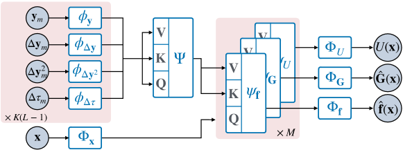
Figure 1: FIM-SDE: Foundation Inference Model for SDE (schematic representation). The (input) context set consists of $K(L-1)$ tuples $\{\mathbf{y},\Delta\mathbf{y},\Delta\mathbf{y}^{2},\Delta\tau\}$ that are projected by the linear $\phi$ layers. The result is processed by a Transformer encoder network $\Psi$ that returns the Context Matrix (Eq. 7 in the main text). The context matrix is used as keys and values to the $M$ Functional Attention Layers $\psi_{\mathbf{f}}$, $\psi_{\mathbf{G}}$ and $\psi_{U}$. The queries are instead the embedded location $\Phi_{\mathbf{x}}^{\theta}(\mathbf{x})$ on which we evaluate the output functions.

Marginalization instabilities. The reader will immediately notice that marginalizing $\mathcal{L}_{1}$ in Eq. 5 (or $\mathcal{L}_{2}$, or $\mathcal{L}_{3}$ of the Appendix) under a uniform distribution, can result in some local contributions dominating the integral — not due to the divergence itself, but rather because of the norm of the involved functions in those regions. One therefore needs a weighting mechanism to balance these contributions over $\mathcal{X}$. We will return to this issue in Section 4.

3.3 Problem Formulation

We are now finally in a position to formulate the problem we aim to solve. Suppose we are given an ordered sequence of $L$ observations $\mathcal{D}^{*}=\{\mathbf{y}_{1}^{*},\mathbf{y}_{2}^{*},\dots,\mathbf{y}_{L}^{*}\}$ of some real-world empirical process $(\mathbf{y}^{*}(t):\mathbb{R}^{+}\rightarrow\mathbb{R}^{d})$ recorded at (non-equidistant) times $0\leq\tau_{1}^{*}<\dots<\tau_{L}^{*}\leq T^{*}$, for some time horizon $T^{*}$. Now assume these observations are generated conditioned on a hidden process $(\mathbf{x}^{*}(t):\mathbb{R}^{+}\rightarrow\mathbb{R}^{d})$, governed by a SDE as that defined in Eq. 1. Our main goal is to construct (non-parametric) neural estimates $\mathbf{\hat{f}}_{\theta}(\mathbf{x}|\mathcal{D^{*}})$ and $\mathbf{\hat{G}}_{\theta}(\mathbf{x}|\mathcal{D}^{*})$, with neural parameters $\theta$ and conditioned on the observations $\mathcal{D}^{*}$, which approximate (i.e. match) the putative drift $\mathbf{f}^{*}(\mathbf{x})$ and diffusion $\mathbf{G}^{*}(\mathbf{x})$ functions that best explain $\mathcal{D}^{*}$ — on some “reasonable” domain $\mathcal{X}\in\mathbb{R}^{d}$.

As we discussed in Section 2, the traditional machine learning solution to this problem invariably involves imposing priors over the target functions $\mathbf{f^{*}}$ and $\mathbf{G^{*}}$, defining variational posteriors over the hidden paths $\mathbf{x^{*}}(t)$, and fitting the model parameters to $\mathcal{D}^{*}$. Our proposal, which we introduce in Section 4, strongly departs from this tradition.

Some comments regarding notation are in order. We denote with $\mathbf{x}(t)$ simulated SDE processes, and with $\mathbf{x}^{*}(t)$ unseen, hidden SDE processes. Similarly, we denote with $\mathbf{y}$ ($\mathbf{y}^{*}$) corrupted paths (empirical, target data). We also denote probability distribution and their densities, as well as random variables and their values, with the same symbols.

4 Foundation Inference Models

In this section, we propose a novel methodology for zero-shot estimation of the drift and diffusion functions that best characterize a target dataset $\mathcal{D}^{*}$ of interest. As outlined in the Introduction, the methodology involves training a neural network model to map a large set of corrupted SDE paths into their a priori-known, target drift and diffusion functions. The latter being sampled from a heuristically constructed synthetic distribution.

The success of this methodology — namely, that a model (pre)trained solely on synthetic data can help understand and predict unseen empirical processes $\mathcal{D}^{*}$ — hinges not only on the inductive biases encoded in the architecture of our model, but also on the family of SDEs represented in the synthetic dataset. Our primary assumption is that, even though we can only consider a very restricted family of drift and diffusion functions, the solution of the SDEs they define can exhibit sufficient complexity to mimic real-world empirical datasets. This assumption resonates with a classical idea popularized by Stephen Wolfram (Wolfram & Gad-el Hak, 2003), but that can be traced back to Kadanoff himself (Kadanoff, 1986, 1987), namely that simple rules can create complex patterns. In the experimental section (Section 5), we empirically demonstrate that our (pre)trained model provides an interpretable picture (i.e. via the estimated drift and diffusion functions) of various synthetic and real-world systems, while also enabling accurate predictions. In what follows, we first introduce our data generation model and then present FIM-SDE, our transformer-based recognition model.

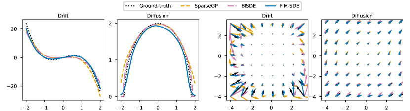
Figure 2: Drift and diffusion function estimation in canonical SDE systems with state-dependent diffusion. Left: Double-well model. Right: Synthetic 2D system from Wang et al. (2022). In contrast to the baselines, FIM-SDE estimates the target functions in zero-shot mode. The (zero-shot) results are in remarkable agreement with the ground-truth.

4.1 Data Generation Model

In this subsection, we introduce the data generation model we use to sample a synthetic dataset of corrupted SDE paths of different dimensionalities. Formally, we can define the probability of observing the noisy sequence $\mathbf{y}_{1},\dots,\mathbf{y}_{L}\in\mathbb{R}^{d}$, at the observation times $0\leq\tau_{1}<\dots<\tau_{L}\leq T$, with $T$ the observation time horizon, as follows

$$\prod\limits_{i=1}^{L} p_{\text{\tiny noise}}\big{(}\mathbf{y}_{i}|\mathbf{x}(\tau_{i}),\mathbf{f},\mathbf{G}\big{)}p_{\text{\tiny FP}}\big{(}\mathbf{x}(\tau_{i})|\mathbf{f},\mathbf{G},\mathbf{x}(0)\big{)}p\big{(}\mathbf{x}(0)\big{)}$$

$$\times p_{\text{\tiny grid}}(\tau_{1},\dots,\tau_{L})p_{\text{\tiny diff}}(\mathbf{G}|d)p_{\text{\tiny drift}}(\mathbf{f}|d).$$ (6)

Let us briefly specify the main components of Eq. 6.

Drift function generation. Drift functions are sampled from the distribution $p_{\text{\tiny drift}}(\mathbf{f}(\mathbf{x})|d)$, which is conditioned on the system dimensionality $d$, and is defined to factorize as $p_{\text{\tiny drift}}(f_{1}(\mathbf{x}))\dots p_{\text{\tiny drift}}(f_{d}(\mathbf{x}))$. We generate drift functions for processes of different dimensionalities — ranging from one until some maximum dimension $d_{\text{\tiny max}}$ — to ensure the applicability of our methodology across systems with dimension within this range (similar approaches were used by Berghaus et al. (2024) and d’Ascoli et al. (2024)). Now, this distribution should represent our beliefs about the class of drift functions we expect to find in nature. In this work, we construct two such distributions: $p^{(1)}_{\text{\tiny drift}}(f(\mathbf{x}))$ and $p^{(2)}_{\text{\tiny drift}}(f(\mathbf{x}))$. The distribution $p^{(1)}_{\text{\tiny drift}}(f(\mathbf{x}))$ is defined over the space of (up to) degree three polynomials with random coefficients, which, albeit simple, covers many important deterministic dynamical systems (as e.g. the famous Lorentz system). The distribution $p^{(2)}_{\text{\tiny drift}}(f(\mathbf{x}))$ is constructed instead over random unary-binary trees following the procedure outlined by Lample & Charton (2020), which enables function composition and thus allows for richer and more expressive dynamics. We invite the reader to check Appendix C.1 for details regarding the implementations of these distributions.

Diffusion function generation. Diffusion functions are sampled from the distribution $p_{\text{\tiny diff}}(\mathbf{G}(\mathbf{x})|d)$, which also factorizes as $p_{\text{\tiny diff}}(g_{1}(\mathbf{x}))\dots p_{\text{\tiny diff}}(g_{d}(\mathbf{x}))$, where the $g_{i}(\mathbf{x})$ correspond to the arguments of the square roots in Eq. 4. State-dependent diffusion is common in financial applications and also plays a role in transport problems in condensed matter physics (see e.g. the classical work by Büttiker (1987)). We define $p_{\text{\tiny diff}}(g(\mathbf{x}))$ over positive polynomials of degree two with random coefficients, which can represent both geometric Brownian motion like processes, and constant diffusion. Appendix C.2 contains the details.

SDE simulation. The term $p_{\text{\tiny FP}}\big{(}\mathbf{x}(t)|,\mathbf{f},\mathbf{G},\mathbf{x}(0)\big{)}$ denotes the instantaneous solution of the Fokker-Planck equation, which evolves the stochastic process at the “macroscopic” (path-ensemble) level, given $\mathbf{f}$, $\mathbf{G}$ and some initial condition $p\big{(}\mathbf{x}(0)\big{)}$. In practice, we define $p\big{(}\mathbf{x}(0)\big{)}$ as the standard normal distribution and simulate individual paths by solving the corresponding SDE using an Euler-Maruyama scheme with discretization $\Delta t$, until the time horizon $T$. Please refer to Appendix C.3 for details.

SDE corruption. Empirical data is noisy, often recorded at irregular time intervals, and can feature inter-observation gaps much larger than the microscopic timescale of the dynamics (i.e. $\Delta\tau\gg\Delta t$). The distribution $p_{\text{\tiny grid}}(\tau_{1},\dots,\tau_{l})$ represents the uncertainty in the sequence of recording times and we implement it by subsampling our SDE solutions through different schemes. Similarly, the distribution $p_{\text{\tiny noise}}\big{(}\mathbf{y}_{i}|\mathbf{x}(t),\mathbf{f},\mathbf{G}\big{)}$ is defined to represent additive Gaussian noise (i.e. the maximum entropy attractor of empirical noise distributions), with a variance that depends on (the characteristic scale of) the stochastic dynamics of the system. Appendix C.4 provides the details.

Table 1: MMD comparisons of FIM-SDE against BISDE (Wang et al., 2022) and SparseGP (Batz et al., 2018). Lower values are better. We report the mean and standard deviation over five (5) runs. The number of “*” denote the number of times the function estimation failed. N/A denote that all estimations (in all runs) failed. Underlined scores are the best scores for a given $\Delta\tau$. Bold scores represent best results overall. All results in this table have been scaled by a factor of 10.

$\Delta\tau$	Model	Double Well	2D-Synt (Wang)	Damped Linear	Damped Cubic	Duffing	Glycolysis	Hopf
0.002	SparseGP	$0.4(4)$*	0.07(4)*	0.07(3)*	0.05(4)	N/A	N/A	0.04(4)
0.002	BISDE	0.01(3)	0.05(4)	$0.13(9)$	N/A	0.05(5)	0.09(2)*	$0.13(8)$
0.002	FIM-SDE	$0.02(1)$	$0.5(2)$	$0.7(1)$	$0.44(9)$	$0.6(2)$	$0.7(4)$	$0.4(1)$
0.01	SparseGP	$0.8(9)$	$0.64(8)$	N/A	N/A	N/A	$0.41(3)$***	$0.7(1)$
0.01	BISDE	N/A	$0.8(1)$	$0.45(7)$	N/A	$0.41(3)$*	$0.6(1)$	$1.0(2)$
0.01	FIM-SDE	0.2(2)	0.06(5)	0.03(2)	0.05(4)	0.03(2)	0.03(2)	0.03(2)
0.02	SparseGP	$1.2(2)$*	$1.2(1)$	N/A	N/A	N/A	N/A	$1.35(8)$
0.02	BISDE	N/A	$1.2(1)$	$0.93(8)$	N/A	N/A	$1.2(1)$	$1.83(4)$*
0.02	FIM-SDE	0.06(2)	0.04(3)	0.05(1)	0.02(2)	0.03(1)	0.02(2)	0.031(4)

4.2 FIM-SDE: a Transformer-based Recognition Model

Above we introduced a data generation model (Eq. 6) for SDEs. Let us suppose that we use this model to generate a large synthetic dataset consisting of tuples of the form $(\mathcal{D},(\mathbf{f},\mathbf{G}))$, where $\mathcal{D}$ denotes a set of $K$ corrupted time series $\{\mathbf{y}_{k1},\dots,\mathbf{y}_{kL}\}_{k=1}^{K}$ of different dimensionalities, and of $L$ observations each, obtained from the SDE defined by the pair $(\mathbf{f},\mathbf{G})$.

We now introduce FIM-SDE, a transformer-based architecture that processes instances of $\mathcal{D}$ to produce estimates $\mathbf{\hat{f}}_{\theta}(\mathbf{x|\mathcal{D}})$, $\mathbf{\hat{G}}_{\theta}(\mathbf{x|\mathcal{D}})$ that approximate the target pair $(\mathbf{f},\mathbf{G})$. This means that FIM-SDE must map $\mathcal{D}$ onto the space of drift and diffusion functions. We will implement this map leveraging concepts from neural operator, specially DeepONets (Lu et al., 2021). However, since each of the tuples $(\mathcal{D},(\mathbf{f},\mathbf{G}))$ corresponds to an SDE characterized by distinct spatial and temporal scales, we first need to normalize $\mathcal{D}$ and renormalize the pair $(\mathbf{f},\mathbf{G})$ accordingly (see Appendix D.1 for details). This normalization trick makes FIM-SDE scale agnostic.

Let $\phi^{\theta}(\cdot)$ and $\Phi^{\theta}(\cdot)$ denote linear projections and feed-forward neural networks, respectively. Let $\psi^{\theta}(\cdot,\cdot,\cdot)$ denote attention layers, and let $\Psi^{\theta}(\cdot,\cdot,\cdot)$ denote Transformer encoders with linear attention (Katharopoulos et al., 2020), both of which take three arguments as inputs (i.e. queries, keys and values). Finally, let $\theta$ denote model parameters.

Context Matrix (Branch-net equivalent). Upon directly inspecting Eqs. 2 and 3, we notice that the values of the drift and diffusion functions at a given location, say $\mathbf{x}$, only depend on transitions that take place in the “neighborhood” of $\mathbf{x}$. In other words, the sequential nature of the data within $\mathcal{D}$ does not seem to encode information relevant to the estimation of the local expectations in Eqs. 2 and 3 (or, at least not directly). We therefore reorganize the data within every set $\mathcal{D}$ into $K(L-1)$ tuples of the form $\mathcal{\tilde{D}}=\{\mathbf{y}_{i},\Delta\mathbf{y}_{i},\Delta\mathbf{y}^{2}_{i},\Delta\tau_{i}\}_{i=1}^{K(L-1)}$, which only keep information about one-step transitions. Let us now define the $n$-dimensional embeddings

$$\mathbf{d}^{\theta}_{i}=\text{concat}\Big{[}\phi^{\theta}_{\mathbf{y}}(\mathbf{y}_{i}),\phi^{\theta}_{\Delta\mathbf{y}}(\Delta\mathbf{y}_{i}),\phi^{\theta}_{\Delta\mathbf{y}^{2}}(\Delta\mathbf{y}^{2}_{i}),\phi^{\theta}_{\Delta\tau}(\Delta\tau_{i})\Big{]}$$

where $i$ runs from 1 to $K(L-1)$ for every element in $\mathcal{\tilde{D}}$, and the linear projections $\phi^{\theta}$ map their inputs onto $\mathbb{R}^{n/4}$. Let now $\mathbf{D}^{\theta}=[\mathbf{d}^{\theta}_{1},\dots,\mathbf{d}^{\theta}_{K(L-1)}]$ denote the $n\times K(L-1)$ matrix of linear embeddings, and define the (self-attentive) context matrix

$$\mathbf{\tilde{D}}^{\theta}=\Psi^{\theta}(\mathbf{D}^{\theta},\mathbf{D}^{\theta},\mathbf{D}^{\theta}),\,\,\text{so that}\,\,\mathbf{\tilde{D}}^{\theta}\in\mathbb{R}^{n\times K(L-1)},$$ (7)

which encodes the entire context data $\mathcal{\tilde{D}}$.

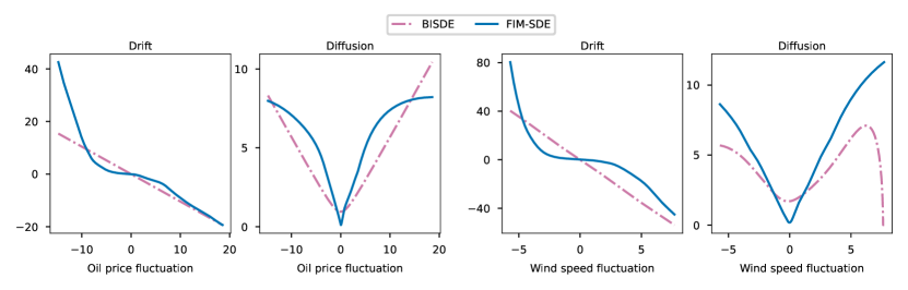
Figure 3: Drift and diffusion function estimation in real-world scenarios. Left: Oil price fluctuations. Right: Wind speed fluctuations. FIM-SDE, which was only trained on synthetic data, remarkably estimates drift and diffusion functions that are in good-agreement with the baselines.

Functional attention mechanism (Trunk-net equivalent). Having encoded the context data $\mathcal{\tilde{D}}$ into $\mathbf{\tilde{D}}^{\theta}$, we now proceed to compute our function estimates by introducing a type of functional attention mechanism. In short, this mechanism takes the embedded location at which we want to evaluate the output function, say $\mathbf{x}$, as the query in a sequence of $M$ attention networks. The keys and values of these networks are instead given by $\mathbf{\tilde{D}}^{\theta}$. To illustrate, we focus on the drift function estimates and compute a sequence of $M+1$ location-dependent embeddings

$$\mathbf{h}_{i}^{\theta}(\mathbf{x}|\mathcal{\tilde{D}})=\psi_{\mathbf{f},i}^{\theta}(\mathbf{h}_{i-1}^{\theta}(\mathbf{x}|\mathcal{\tilde{D}}),\mathbf{\tilde{D}}^{\theta},\mathbf{\tilde{D}}^{\theta}),$$

with $i$ running from $1$ until $M$, and $\mathbf{h}_{0}^{\theta}(\mathbf{x}|\mathcal{\tilde{D}})=\mathbf{h}_{0}^{\theta}(\mathbf{x})=\Phi^{\theta}_{\mathbf{x}}(\mathbf{x})$. From here, we define

$$\mathbf{\hat{f}}_{\theta}(\mathbf{x}|\mathcal{\tilde{D}})=\Phi^{\theta}_{\mathbf{f}}(\mathbf{h}^{\theta}_{M}(\mathbf{x}|\mathcal{\tilde{D}})).$$ (8)

The calculation of $\mathbf{\hat{G}}_{\theta}(\mathbf{x}|\mathcal{\tilde{D}})$ is analogous.

Target objective. We optimize the model parameters $\theta$ to minimize the divergence between our estimates and the target function pair $(\mathbf{f},\mathbf{G})$ on our “reasonable” domain $\mathcal{X}$. For concreteness, we choose $\mathcal{L}_{1}$ in Eq. (5) of Section 3 and write

$$\mathcal{L}=\underset{\mathbf{x}\sim\mathcal{U}(\mathcal{X})}{\mathbb{E}}\underset{p(\mathcal{D})}{\mathbb{E}}\left[e^{-U_{\theta}(\mathbf{x},\mathcal{D})}\mathcal{L}^{\theta}_{1}(\mathbf{x,\mathcal{D}})+U_{\theta}(\mathbf{x},\mathcal{D})\right],$$ (9)

where we made explicit the dependence of $\mathcal{L}_{1}$ on both data and trainable parameters, $\mathcal{U}$ denotes uniform distribution, and $p(\mathcal{D})$ labels the generative model of Eq. 6. The learnable function $U_{\theta}(\mathbf{x},\mathcal{D})$ is introduced to address the scaling problem we sketched in Section 3.2, and can be understood as an (epistemic) uncertainty estimator (see e.g. Appendix B in Karras et al. (2024)). Similar to our estimation of $\mathbf{\hat{f}}_{\theta}$ and $\mathbf{\hat{G}}_{\theta}$, we implement $U_{\theta}$ with a third set of $M$ attention functions $(\psi^{\theta}_{U,1},\dots,\psi^{\theta}_{U,M})$, but only back-propagate up to $\mathbf{\tilde{D}}^{\theta}$. Figure 1 illustrates the FIM-SDE architecture.

5 Experiments

In this section, we test our methodology on two classes of experiments, namely seven canonical SDE systems of varying complexity and different dimensionalities, and three experimental, real-world systems. The latter consist of human motion and oil price and wind speed fluctuation records, each of which feature noise signals of very varied nature. We use one and the same FIM-SDE to estimate the drift and diffusion functions of each of these systems in zero-shot mode. In other words, we do not modify the (pre)trained weights of FIM-SDE before applying it to any of our target datasets.

We (pre)trained a 20M-parameter FIM-SDE on a dataset of 700K SDEs spanning multiple dimensionalities. Specifically, we constructed three, two and one-dimensional SDEs appearing in a 3:2:1 ratio. Of these, 600K SDEs have polynomial drifts, while the remainder involve more complex drift structures based on function compositions — that is, they are sampled from $p_{\text{\tiny drift}}^{(1)}(f(\mathbf{x}))$ and $p_{\text{\tiny drift}}^{(2)}(f(\mathbf{x}))$, respectively. The diffusion functions in the ensemble were all sampled from $p_{\text{\tiny diff}}(g(\mathbf{x}))$. Finally, the number of paths (i.e. realizations) processed by the model during (pre)training is uniformly distributed between one and one hundred (because we do not know a priori how much data we will have access to in practice). Additional information regarding the (pre)training data distribution, model architecture and hyperparameters, training details and ablation studies can all be found in Appendix C and D.

Metrics. We evaluate the quality of our estimated drift and diffusion functions primarily using three methods. First, we assess them visually by plotting the corresponding vector fields on predefined, uniform grids. Second, when ground-truth functions are available, we compute the mean squared error (MSE) of our estimates on the predefined grid, against the ground-truth values. Third, we evaluate the quality of sampled realizations from the estimated SDEs by comparing them against held-out trajectories. To quantify this, we compute the maximum mean discrepancy (MMD) between path ensembles, with respect to the signature kernel introduced by Király & Oberhauser (2019) (see Appendix E for some implementation details).

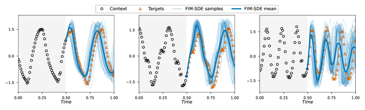
Figure 4: Zero-shot forecasting with FIM-SDE of the first 3 PCA components in the motion capture experiment. FIM-SDE infers the vector fields from the context points (black circles) and predicts the targets (red triangles) by sampling paths starting at the last observation. The average prediction is displayed in bold.

Baselines. We compare our findings against two baselines, namely the Bayesian non-parametric model of Batz et al. (2018), and the sparse Bayesian and symbolic solution of Wang et al. (2022). Let us refer to them as SparseGP and BISDE, respectively. For SparseGP, we implemented the Sparse Gaussian Process for Dense Observations method following Batz et al. (2018) (see Appendix F.1). For BISDE, we used the open-source implementation of Wang et al. (2022), and modified its library of functions to only include monomials up to order three, together with sine and exponential functions whose arguments also consists of monomials, up to order three. This way, we (approximately) maintain the same inductive biases encoded into our synthetic datasets, thereby ensuring fairness of comparison. Both baselines assume complete access to the “clean” state of the systems, meaning that they are expected to perform well on dense data (that is, $\Delta\tau\simeq\Delta t$, with $\Delta t$ the “microscopic” time scale of the target process) without any noise corruption.

5.1 Canonical SDE systems

In this subsection, we study seven widely different SDE systems, which we define in Appendix F.2, among which one finds the classical (one-dimensional) double-well system with state-dependent diffusion — a common case study in the Bayesian community. We first solve each system using an Euler-Maruyama step of $(\Delta t=)0.002$, thereby setting the “microscopic” time scale of the system(s), until a time horizon $T=10$. In contrast, FIM-SDE was (pre)trained on corrupted SDE paths whose inter-observation time distribution $p(\Delta\tau)$ peaks at around $0.08$ (see Appendix C.4 for details). To assess the robustness of FIM-SDE to varying inter-observation times, we construct three different experiments per target SDE. The first preserves the “microscopic” time scale with $\Delta\tau=\Delta t=0.002$. The other two use coarser inter-observation times, namely $\Delta\tau=0.01$ and $\Delta\tau=0.02$ (still shorter than the mean $\Delta\tau$ within our synthetic distributions), but are all defined to contain the same number of observations. We make use of FIM-SDE, as well as our baselines, to estimate the (hidden) ground-truth drift and diffusion functions, and repeat the experiments five times. That is, we generate five independent datasets with the features described above. Clearly, both baselines need to be trained from scratch on all these systems and configurations. FIM-SDE is instead used off-the-shelf, with no modification throughout all experiments.

Table 1 contains the MMD calculations for all three experiments and all seven SDE systems, averaged over the five runs. The emergent picture is clear. FIM-SDE outperforms all baselines in every dataset at the coarser scales ($\Delta\tau=0.01$, $0.02$). At the finer, “microscopic” scale BISDE dominates. Surprisingly both BISDE and SparseGP often estimate SDEs with no solution. FIM-SDE is stable in this regard. Figure 2 displays the inferred drift and diffusion functions for the double-well system and the two-dimensional synthetic system of Wang et al. (2022) (Eqs. 37 and 38 in the Appendix) by all models, at the setting they perform best. FIM-SDE estimations are in excellent agreement with the ground-truth. Table 2 in the Appendix provides a consistent and complementary picture.

5.2 Real-world systems

In this subsection, we use FIM-SDE to understand wind speed and oil price fluctuations, comparing our findings against the results of Wang et al. (2022), who originally collected and analyzed these datasets (see Appendix F.3). Both systems exhibit inherent stochasticity. For example, wind speed fluctuations have recently been described using Ornstein-Uhlenbeck (OU) processes with linear diffusion (Loukatou et al., 2018). Similarly, oil price fluctuations have been modeled as geometric Brownian motion (GBM), which also assumes linear diffusion (Noh et al., 2016; Yang & He, 2024). We optimize BISDE on both datasets and directly apply FIM-SDE to them. Figure 3 demonstrates that, at small fluctuation scales, both models generally align with GBM but, at larger scales, exhibit additional structure. However, Table 3 demonstrates that our estimates provide a better description of the empirical data.

We conclude this section by demonstrating that FIM-SDE can also perform zero-shot forecasting of human motion recordings, using only about 50(!) observations as context data (see Figure 4). We refer the reader to Appendix F.4 for details on the dataset and to Table 4 for preliminary comparisons with other neural models.

6 Conclusions

In this work, we introduced a novel methodology for zero-shot estimation of drift and diffusion functions from data. We empirically demonstrated that one and the same FIM-SDE was able to correctly characterized various synthetic and real-world systems of different dimensionalities, while performing on par with SOTA models trained on the target datasets. The main limitation of our methodology is naturally imposed by our synthetic training distributions. Indeed, we empirically verified in Tables 1 and 2 that evaluating FIM-SDE on systems whose microscopic scale $\Delta t$ is out-of-distribution can lead to weaker estimates. Future work will broaden $p(\Delta\tau)$ within our training set, and investigate how to minimize its role through novel instance normalization mechanisms.

Impact Statement

FIM-SDE can have a strong impact in the scientific community, specially from the point of view of accessibility. The traditional machine learning paradigm requires practitioners to have access to high-quality datasets and substantial computational resources. It also requires them to have the experience and expertise to train state-of-the-art models from scratch. Foundation models — like FIM-SDE — do not necessarily require machine expert knowledge, which implies that they (foundation models) can be used by a broader community of scientists and engineers.

Appendix A Relation with Early Amortized and Meta-learning Approaches

On the concept of amortization. Our methodology can be understood as an amortization of the probabilistic inference process (of the drift and diffusion functions) through a single neural network, and is therefore akin to the works of Stuhlmüller et al. (2013), Heess et al. (2013) and Paige & Wood (2016).

Rather than treating, as these previous works do, our (pre)trained models as auxiliary to Monte Carlo or expectation propagation methods, we employ them to directly estimate the drift and diffusion functions from various synthetic, simulation and experimental datasets, without any parameter fine-tuning.

On conditional neural network models and meta-learning. Different from the “foundation models” trained on synthetic datasets (like FIM-SDE), conditional neural network models — such as the neural statistician (Edwards & Storkey, 2016; Hewitt et al., 2018) or members of the neural process family (Garnelo et al., 2018b, a; Kim et al., 2019) — are trained across sets of different, albeit related datasets, each assumed to share a common context latent variable

These meta-learning models are trained exclusively on (sets of) datasets from their target domains, rendering both their optimized weights and the representations they can infer (that is, their latent variables) problem/data specific.

In contrast, our method maintains the same network parameters and representation semantics throughout all experiments. The representations consistently correspond to drift and diffusion functions of SDEs, regardless of the target dataset.

Appendix B Alternative Objective Functions for SDE Matching

In this section, we provide the explicit expression two alternative divergences between SDE processes.

Divergence 2. We can estimate the Kullback-Leibler divergence between the conditional probabilities of transitioning from state $\mathbf{x}$ into (some) state $\mathbf{x}^{\prime}$, over a time interval $\Delta t$, as determined by each function pair — that is, $p(\mathbf{x}^{\prime},t+\Delta t|\mathbf{x},t,\mathbf{\hat{f}},\mathbf{\hat{G}})$ and $p(\mathbf{x}^{\prime},t+\Delta t|\mathbf{x},t,\mathbf{f},\mathbf{G})$.

For small $\Delta t$ these conditional distributions are approximately Gaussian, which allows us to define the second divergence as

$$\mathcal{L}_{2}(\mathbf{x})=\frac{1}{2}\Big{[}\sum_{i=1}^{D}\frac{(\hat{f}_{i}(\mathbf{x})-f_{i}(\mathbf{x}))^{2}\Delta t}{g_{i}(\mathbf{x})}+\frac{\hat{g}_{i}(\mathbf{x})}{g_{i}(\mathbf{x})}+\log g_{i}(\mathbf{x})-\log\hat{g}_{i}(\mathbf{x})-1\Big{]}.$$ (10)

Divergence 3. We can compute the log-likelihood of the short-time transitions induced by one function pair, say $(\mathbf{f},\mathbf{G})$, with respect to the second pair. Specifically, we write

$$\mathcal{L}_{3}(\mathbf{x})=-\frac{1}{2}\,\mathbb{E}_{p(\mathbf{x^{\prime}}|\mathbf{x},\mathbf{f},\mathbf{G})}\Big{[}\sum_{i=1}^{D}\frac{(x_{i}^{\prime}-x_{i}-\hat{f}_{i}(\mathbf{x})\Delta t)^{2}}{\hat{g}_{i}(\mathbf{x})\Delta t}-\log\hat{g}_{i}(\mathbf{x})\Delta t\Big{]},$$ (11)

where $p(\mathbf{x^{\prime}}|\mathbf{x},\mathbf{f},\mathbf{G})$ denotes the short-time transition probability according to the function pair $(\mathbf{f},\mathbf{G})$.

Interestingly, if we were to modify $(\mathbf{\hat{f}},\mathbf{\hat{G}})$ to align with $(\mathbf{f},\mathbf{G})$ according to Eq. 11, this would imply that $(\mathbf{\hat{f}},\mathbf{\hat{G}})$ must approximate the local (in space) noise generated by $(\mathbf{f},\mathbf{G})$. This process is analogous to how generative diffusion models are trained to match noise locally in time (Ho et al., 2020).

Appendix C Synthetic Data Generation Model: Details

C.1 Distribution Over Drift Functions

In this subsection, we construct two distributions over the components of the drift function.

Distribution $p^{(1)}_{\text{\tiny drift}}(f(\mathbf{x}))$ over degree three polynomials. Let us describe our sampling scheme for polynomials of degree three (or less), which define the components of a $D\leq D_{\text{\tiny max}}$ dimensional process. A polynomial is uniquely defined by a finite set of monomials with non-zero coefficients, and coefficients for these monomials. For a single polynomial, our procedure first samples such set of monomials, and then samples (a.s.) non-zero coefficients for these monomials:

1. Sample the number of monomial degrees $N_{\text{\tiny deg}}\sim\mathcal{U}[1,\dots,D_{\text{\tiny max}}]$ included in the polynomial.

2. Sample $\{d_{1},\dots,d_{N_{\text{\tiny deg}}}\}\sim\mathcal{U}[\mathcal{P}_{N_{\text{\tiny deg}}}[\{0,\dots,D\}]]$, the set of monomial degrees included in the polynomial.

3. For each $i\in\{1,\dots,N_{\text{\tiny deg}}\}$, sample $N_{\text{\tiny mon}}^{i}\sim\mathcal{U}[1,\dots,\binom{d_{i}+D-1}{d_{i}}]$, the number of monomials of degree $d_{i}$ included in the polynomial.

4. For each $i\in\{1,\dots,N_{\text{\tiny deg}}\}$, sample from $\mathcal{U}[\mathcal{P}_{N_{\text{\tiny mon}}^{i}}[\{x^{\alpha}|\left|\alpha\right|=d_{i}\}]]$, the subset of monomials of degree $d_{i}$ included in the polynomial.

5. Sample the coefficients for the included monomials from $\mathcal{N}(0,1)$.

The uniform distributions cover a broad range of degree three polynomials, while the hierarchical sampling scheme ensures some sparsity (regarding monomials with non-zero coefficients) and correlation between monomials of the same degree throughout the whole dataset

Distribution $p^{(2)}_{\text{\tiny drift}}(f(\mathbf{x}))$ over unary-binary trees. We simply follow the data generation procedure of d’Ascoli et al. (2024) (Section 3), but restrict the unary operators to: $\sin$, $\exp$ and $x^{2}$. In other words, we replaced the inverse function with the exponential function. These general random unary-binary method for function construction was introduced by Lample & Charton (2020).

C.2 Distribution Over Diffusion Functions

In this subsection, we define the distribution $p_{\text{\tiny diff}}(g(\mathbf{x}))$ over the components of the diffusion functions.

Recall from (4) that we only consider diagonal diffusion matrices, with components of the form $\sqrt{g(\mathbf{x})}$ for some non-negative function $g$. Guided by some of our target processes, we first sample $\tilde{g}$ as a polynomial of maximal degree $2$, using the procedure described in Appendix C.1. Because $\tilde{g}$ can attain negative values, we define the (sampled) component function by

$$g(\mathbf{x})=\max\left(0,\tilde{g}(\mathbf{x})\right).$$ (12)

Note that some diffusion component functions sampled by this procedure contain (large) regions with low, or even zero diffusion (e.g. when $\tilde{g}$ is a constant of negative value). In practice, we found that our trained model can therefore also approximate (almost) deterministic systems.

C.3 SDE simulations

In this subsection we expatiate upon our simulation procedure.

Given the drift function $\mathbf{f}(\mathbf{x})$ and the diffusion function $\mathbf{G}(\mathbf{x})$, sampled as described in sections C.1 and C.2, we solve the corresponding SDE (that is, sampled the paths) using the Euler–Maruyama method. For performance reasons, we use the julia programming language Bezanson et al. (2017) and the solver implementation of the DifferentialEquations.jl package Rackauckas & Nie (2017b, a).

For each equation, we realize $K=100$ simulations. Concretely, we sample set of $K$ initial states from $\mathcal{N}(0,1)$ and simulate the equation with discretization $\Delta t=0.004$ in the time interval $[0,T]$, where we set $T=10$. Should the simulation of a single path fail (e.g. include NaN or Inf values), we discard the equation, sample a new equation and repeat the simulation process. Similarly, we discard diverging systems by discarding equations, if the absolute value of one component of one path exceeds a threshold value of $100$.

C.4 SDE corruption

In this subsection we describe how we implement the distribution $p_{\text{\tiny grid}}(\tau_{1},\dots,\tau_{l})$ (over the sequence recording times) and $p_{\text{\tiny noise}}\big{(}\mathbf{y}_{i}|\mathbf{x}(t),\mathbf{f},\mathbf{G}\big{)}$ (over the optional corruption of the process values).

Regular observation grids. By default, we consider regular, coarse observation grids. To realize such observations of our sampled equations, we subsample the fine grid simulations from Appendix C.3 by a factor of $20$, yielding $L=128$ observations on the regular grid in $[0,10]$. In other words, the sequences are (by default) recorded with a regular inter-observation gap of $\Delta\tau=0.08$.

Irregular observation grids. To accommodate applications with irregular inter-observation gaps, we subsample these regular grids with an additional sampling scheme using the Bernoulli distribution. Given the regular, coarse observations of a process, we sample a Bernoulli survival probability $\eta\sim\mathcal{U}[0.9,1]$. The irregular observation grid for a given process are then realized by sampling the Bernoulli distribution with survival probability $\eta$ at each observation.

Additive Gaussian noise. To make the model more robust, e.g. for real world applications, we corrupt the (clean) observations $\{\mathbf{x}_{i}\}_{i=1}^{K\times(L-1)}$ of a process $(\mathbf{f},\mathbf{G})$ by additive Gaussian noise. The standard deviation is determined relative to the observed values. Concretely, let us define the component-wise range of the process:

$$r({\mathbf{x}(t),\mathbf{f},\mathbf{G}})=\frac{1}{2}\left(\max_{\begin{subarray}{c}i=1,\dots,K\times(L-1)\end{subarray}}\mathbf{x}_{i}-\min_{\begin{subarray}{c}i=1,\dots,K\times(L-1)\end{subarray}}\mathbf{x}_{i}\right)$$ (13)

To realize the additive Gaussian noise, we first sample a noise scale $\sigma({\mathbf{x}(t),\mathbf{f},\mathbf{G}})\sim\mathcal{U}[0,0.1]$ for the given (clean) observations of a process. Then, each observation is corrupted by samples from $\mathcal{N}(0,\sigma({\mathbf{x}(t),\mathbf{f},\mathbf{G}})r({\mathbf{x}(t),\mathbf{f},\mathbf{G}}))$. In other words:

$$p_{\text{\tiny noise}}\big{(}\mathbf{y}_{i}|\mathbf{x}(t),\mathbf{f},\mathbf{G}\big{)}=\mathcal{N}(\mathbf{x}_{i},\sigma({\mathbf{x}(t),\mathbf{f},\mathbf{G}})r({\mathbf{x}(t),\mathbf{f},\mathbf{G}}))$$ (14)

In practice, each corruption scheme is applied to a third of the total training dataset. These corruptions might overlap, i.e. observations of a process can be noisy and on an irregular grid.

Note that a (Course & Nair, 2023) employ a similar relative additive noise scheme in some of their experiments on synthetic data. However, they define the range of a process based on the associated ODE process, i.e. with zero diffusion.

Appendix D Foundation Inference Models: Details

D.1 Instance Normalization and Change of variable formulas (Input Pre-processing, Outputs Post-processing)

Observation sequences on different dynamical process are naturally characterized by different spatial and temporal length scales. To handle such sequences in a consistent manner, we introduce component-wise instance normalization transformations. We pre-process the inputs to our model before application, and post-process the outputs according to the relevant change of variables formulas.

Continuing the notation from 4.2, let the data $\mathcal{D}^{\prime}=\{\mathbf{y}_{i},\Delta\mathbf{y}_{i},\Delta\mathbf{y}^{2}_{i},\Delta\tau_{i}\}_{i=1}^{K(L-1)}$ and a location $\mathbf{x}$ be the inputs of FIM-SDE. We consider linear normalization transformations, so the normalizations of $\Delta\mathbf{y}$, $\Delta\mathbf{y}^{2}$ and $\Delta\tau$ are implied by the normalization transformations of $\mathbf{y}$ and $\tau$.

Spatial instance normalization. Before applying our model, we standardize the observations $\{\mathbf{y}_{i}\}_{i=1}^{K(L-1)}$ component-wise. Let $y_{ij}$ denote the $j$-th component of $\mathbf{y}_{i}$. Then the $j$-th component of the observations are standardized using

$$\bar{y}_{i}=\frac{1}{K(L-1)}\sum_{j=1}^{K(L-1)}y_{ij}\quad\text{and}\quad s_{i}=\sqrt{\frac{1}{K(L-1)}\sum_{j=1}^{K(L-1)}(y_{ij}-\bar{y}_{i})^{2}}\quad.$$ (15)

It is important to apply the same standardization transformation to the location $\mathbf{x}$, because they are elements of the now transformed domain.

Temporal instance normalization. The absolute time $\tau_{i}$of an observation is not an input of our model. We therefore normalize $\Delta\tau_{i}$ directly. However, during application (as well as some part of our training data), $\Delta\tau_{i}$ might be constant, i.e. the input observations are on a regular grid. Moreover, $\Delta\tau_{i}$ might differ (vastly) between applications, even if all of them are on a regular grid. We therefore only centralize $\{\Delta\tau_{i}\}_{i=1}^{K(L-1)}$ around a target value, while keeping the inter-observation gaps positive for interpretability.

Let $\Delta\tau_{\text{\tiny tar}}=0.01$ be a target inter-observation gap after normalization and

$$\bar{\ln}_{\Delta\tau}=\frac{1}{K(L-1)}\sum_{j=1}^{K(L-1)}\ln\Delta\tau_{ij}$$ (16)

the mean of $\{\ln\Delta\tau_{i}\}_{i=1}^{K(L-1)}$. Then we normalize the inter-observation gaps by applying the transformation

$$\Delta\tau\mapsto\Delta\tau_{\text{\tiny tar}}\exp(-\bar{\ln}_{\Delta\tau})\Delta\tau\quad.$$ (17)

In other words, we center $\{\ln\Delta\tau_{i}\}_{i=1}^{K(L-1)}$ at $\ln\Delta\tau_{\text{\tiny tar}}$. Note that the (unique) corresponding transformation of absolute time, that retains $\tau=0$, is

$$\tau\mapsto\Delta\tau_{\text{\tiny tar}}\exp(-\bar{\ln}_{\Delta\tau})\tau\quad.$$ (18)

Change of variable formulas. Let us briefly recall the change of variable formulas relevant for our setting. Consider now $dx(t)=f(x(t))dt+G(x(t))dW(t)$, a one-dimensional SDE with purely state-dependent drift and diffusion functions. The normalization transformations described above (and also their inverses) are linear maps $\tilde{x}(x)=\alpha x+\beta$ (spatial transformation) and $\tilde{t}(t)=\gamma t$ (temporal transformation) for some $\alpha,\beta,\gamma\in\mathbb{R}$. Then the equation of the transformed process $d\tilde{x}(x)(\tilde{t})$ is

$$d\tilde{x}(x)(\tilde{t})=\frac{\alpha}{\gamma}f(x(\gamma^{-1}\tilde{t}))d\tilde{t}+\frac{\alpha}{\sqrt{\gamma}}G(x(\gamma^{-1}\tilde{t}))dW(\tilde{t})$$ (19)

according to Ito’s formula and Theorem 8.5.7 in Øksendal (2010).

Inverse vector fields transformation. Let $\mathbf{\hat{f}}_{\theta}(\mathbf{x}|\mathcal{D}^{\prime})$ and $\mathbf{\hat{G}}_{\theta}(\mathbf{x}|\mathcal{D}^{\prime})$ be the vector field values at location $x$, estimated by FIM-SDE, given instance normalized inputs. As the inputs have been instance normalized, these outputs define processes in the normalized domain. By the change of variables formulas above, the corresponding process in the data domain is defined by the drift and diffusion

$$\mathbf{\hat{f}}_{\theta}(\mathbf{x}|\mathcal{D}^{\prime})s_{i}\Delta\tau_{\text{\tiny tar}}\exp(-\bar{\ln}_{\Delta_{\tau}}),\quad\mathbf{\hat{G}}_{\theta}(\mathbf{x}|\mathcal{D}^{\prime})s_{i}\sqrt{\Delta\tau_{\text{\tiny tar}}\exp(-\bar{\ln}_{\Delta_{\tau}})}\quad.$$ (20)

D.2 Model Architecture

In this section, we provide some more details about the architecture of the single FIM-SDE, all presented experiments were conducted with.

We fix a hidden size $E=256$ for all embeddings throughout the different parts of the model.

All features are embedded with linear layers $\phi_{\cdot}^{\theta}$ to dimension $\frac{E}{4}$, s.t. their concatenated embedding $\mathbf{d}_{i}^{\theta}$ is of the desired size $E$. The embedded features are further encoded by the Transformer encoder with linear attention $\Psi^{\theta}$. It consists of $2$ layers and attention dimension $E$.

Each location is a single input, encoded by another linear layer $\Phi_{x}^{\theta}$ to $E$ dimensions.

The trunk-net equivalent functional attention mechanism first applies $M=8$ attention blocks (including residual feed-forward layers). The final embeddings $\mathbf{h}_{\cdot,M}^{\theta}(\mathbf{x})|D^{\prime})$ are then projected to output dimension $3$ by feed-forward networks with $2$ hidden layers of dimension $E$.

D.3 Training Procedure

We train FIM-SDE with AdamW (Loshchilov & Hutter, 2017), using learning rate $1e^{-5}$ and weight decay $1e^{-4}$. For stability of training (some ground-truth vector field values are large, even after instance normalization), we used gradient clipping with norm $1$.

Memory requirements are quite large, as we provide the model as much as $100$ paths of length $128$ during training. Therefore, we utilize four A100 40GB GPUs to train with a batch size of $64$.

In each batch, we sample the number of paths passed to the model from $\mathcal{U}[0,100]$, s.t. the FIM-SDE can be applied to datasets of many sizes. Moreover, for each equation in a batch, we randomly select $32$ locations to compute the loss $\mathcal{L}_{1}(\mathbf{x})$ of (5) on.

Appendix E Maximum Mean Discrepancy

The Maximum Mean Discrepancy (MMD) is a non-parametric statistical test used to compare two probability distributions Gretton et al. (2012). The objective of MMD is to measure the difference between two distributions, $P$ and $Q$, based on samples drawn from these distributions. MMD employs kernel methods to map the data into a high-dimensional feature space where linear methods can be effectively applied.

We use Ksig Tóth et al. (2025) which is a library to compute signature kernels for time series. Using the RBF-kernel and 5 signature levels, we obtain a signature kernel $k(x,y)$. The MMD between two sets of samples $\{x_{i}\}_{i=1}^{n}\sim P$ and $\{y_{j}\}_{j=1}^{m}\sim Q$ can then by computed as

$$\text{MMD}^{2}(P,Q)\approx\frac{1}{n(n-1)}\left(\sum_{i\neq j}k(x_{i},x_{j})+\sum_{i\neq j}k(y_{i},y_{j})\right)-\frac{2}{n^{2}}\sum_{i,j}k(x_{i},y_{j})\,.$$ (21)

To compute our performance metrics, we choose $x_{i}$ to be samples from the ground truth SDE and $y_{i}$ to be samples derived from the inferred equations of the selected model. For this, we are using $K=100$ paths.

Appendix F Experiments: Details

F.1 SparseGP Drift and Diffusion Estimation

Sparse Approximation

We employed the Sparse Gaussian process (GP) approximation (Batz et al., 2018) to estimate the drift function and diffusion $\mathbf{f}(\mathbf{x})$ and $\mathbf{G}(\mathbf{x})$ in the (SDEs). A specific covariance kernel $\kappa_{\theta}(z_{i},z_{j})$ (such as the RBF) is prescribed per dimension. In order to reduce computational burden we introduce inducing points, these can be thought of as pseudo-observations of the function at $S$ locations $\mathbf{z}=[z_{1},\ldots,z_{S}]$. The drift (or diffusion) estimator is then given by:

$$h_{i}(\mathbf{x})=[\mathbf{k}(\mathbf{x})^{i}]^{\top}\left(I+\gamma^{i}\mathbf{K}_{s}^{i}\right)^{-1}\Delta t(\pi^{i})^{\top}(\mathbf{g}^{i})^{-1}\mathbf{u}^{i},$$ (22)

Here, $[\mathbf{K}^{i}_{s}]_{vw}=\kappa_{\theta}(\mathbf{z}_{v},\mathbf{z}_{w})$ and $[\mathbf{k}(\mathbf{x})^{i}]_{v}=\kappa_{\theta}(\mathbf{x},\mathbf{z}_{v})$, $\pi^{j}=\mathbf{K}_{Ns}^{i}(\mathbf{K}_{s}^{i})^{-1}$ provides the projection onto the inducing points, and $\gamma^{i}=\Delta t(\pi^{i})^{\top}(\mathbf{g}^{i})^{-1}\pi^{i}$ controls the influence of the inducing points. $\mathbf{g}^{i}$ is a diagonal matrix composed by the functions $g(\mathbf{x})$ for the drift estimation, and corresponds to a nuance parameter for the diffusion estimator. This sparse approximation replaces the full kernel matrix with a reduced matrix involving only the inducing points, significantly reducing computational cost from $\mathcal{O}(n^{3})$ to $\mathcal{O}(m^{3})$, where $m\ll n$. This approach ensures efficient inference even for large datasets while preserving the flexibility of nonparametric drift estimation.

Drift and Diffusion Estimation for Dense Observations

For densely observed data, the drift function $h_{i}(\mathbf{x})=f_{i}(\mathbf{x})$ is estimated using GP regression, where the observed increments

$$u_{i}(t_{k})=\frac{y_{i}(t_{k}+\Delta t)-y_{i}(t_{k})}{\Delta t},$$ (23)

are treated as noisy observations of the drift. On the other hand, the diffusion function $h_{i}(\mathbf{x})=g_{i}(\mathbf{x})$ is estimated using the squared increments:

$$\tilde{u}_{i}(t_{k})=\frac{(y_{i}(t_{k}+\Delta t)-y_{i}(t_{k}))^{2}}{\Delta t},$$ (24)

which represent the conditional variance of the observed process. The diffusion estimator follows from the expression:

$$g^{*}_{i}(\mathbf{x})=\lim_{\Delta t\to 0}\frac{1}{\Delta t}\mathbb{E}[(x_{i}(t+\Delta t)-x_{i}(t))^{2}|x_{i}(t)=\mathbf{x}].$$ (25)

To estimate $g^{*}(x)$, GP regression is applied to the squared increments $\tilde{y}_{i}$, treating them as noisy observations of the conditional variance.

In our experiments, we made use of Polynomial kernel for drift estimation, RBF for diffusion. We used a grid search optimizing the data likelihood an selected inducing points in regions of high path density as specified by (Batz et al., 2018).

F.2 Canonical SDE systems

We compare FIM-SDE against two methods: the Bayesian non-parametric method of Batz et al. (2018) and the sparse Bayesian learning model of Wang et al. (2022). To study their performance in fine and coarse grid observations, we simulate well known processes, extracted from (Batz et al., 2018), (Course & Nair, 2023) and (Wang et al., 2022):

1. Double-well diffusion model with state-dependent diffusion:

   $$dx=4(x-x^{3})dt+\sqrt{\max(4-1.25x^{2},0)}dW(t).$$ (26)

   A process from (Batz et al., 2018). We set the initial state to $x(0)=0$.

2. Damped linear oscillator:

   $$dx_{1} = -(0.1\,x_{1}-2.0\,x_{2})dt+\,dW(t),$$ (27)

   $$dx_{2} = -(2.0\,x_{1}+0.1\,x_{2})dt+\,dW(t),$$ (28)

   A process from (Course & Nair, 2023). The initial state is $x(0)=[2.5,-5]$.

3. Damped cubic oscillator:

   $$dx_{1} = -(0.1\,x_{1}^{3}-2.0\,x_{2}^{3})dt+\,dW(t),$$ (29)

   $$dx_{2} = -(2.0\,x_{1}^{3}+0.1\,x_{2}^{3})dt+\,dW(t),$$ (30)

   A process from (Course & Nair, 2023). The initial state is $x(0)=[0,-1]$. (Course & Nair, 2023)

4. Duffing oscillator:

   $$dx_{1} = x_{2}dt+\,dW(t),$$ (31)

   $$dx_{2} = -(x_{1}^{3}-x_{1}+0.35\,x_{2})dt+\,dW(t),$$ (32)

   A process from (Course & Nair, 2023). The initial state is $x(0)=[3,2]$.

5. Selkov glycolysis:

   $$dx_{1} = -(x_{1}-0.08\,x_{2}-x_{1}^{2}x_{2})dt+\,dW(t),$$ (33)

   $$dx_{2} = (0.6-0.08\,x_{2}-x_{1}^{2}x_{2})dt+\,dW(t),$$ (34)

   A process from (Course & Nair, 2023). The initial state is $x(0)=[0.7,1.25]$. (Course & Nair, 2023)

6. Hopf bifurcation:

   $$dx_{1} = (0.5\,x_{1}+x_{2}-x_{1}(x_{1}^{2}+x_{2}^{2}))dt+\,dW(t),$$ (35)

   $$dx_{2} = (-x_{1}+0.5\,x_{2}-x_{2}(x_{1}^{2}+x_{2}^{2}))dt+\,dW(t),$$ (36)

   A process from (Course & Nair, 2023). The initial state is $x(0)=[2,2]$.

7. 2D synthetic system:

   $$dx_{1} = (x_{1}-x_{2}-x_{1}x_{2}^{2}-x_{1}^{3})dt+\sqrt{1+x_{2}^{2}}\,dW(t),$$ (37)

   $$dx_{2} = (x_{1}+x_{2}-x_{1}^{2}x_{2}-x_{2}^{3})dt+\sqrt{1+x_{1}^{2}}\,dW(t).$$ (38)

   A process from Wang et al. (2022). The initial state is $x(0)=[1.5,1.5]$.

For context data $\mathcal{D}$ we simulate the different processes with a dense time step of $\Delta t=0.002$. We then record every $k=1,5,10$ dense steps where $k=\tau/\Delta t$ (we report only the $\tau=0.002,0.01,0.02$) and simulate until we observe 5000 points. For each process and each $\tau$, we repeat this sampling $5$ times, to report a standard deviation for the performance of each model.

Additionally, we sample $100$ paths of length $500$ of each system with $\Delta\tau=0.002$. These paths are used as references to compute the MMD metric of Appendix E.

Let us now briefly describe the experimental setup. We apply FIM-SDE and the two baseline models for all processes and all $\Delta\tau$ and infer an estimated process. We then simulate $100$ paths of length $500$ of the inferred equations, starting from from a fixed set of initial states. Importantly, these simulations are performed with $\Delta\tau=0.002$, independent of the $\Delta\tau$ from the observations. Moreover, we evaluate the estimated vector fields on a fixed grid.

We compare the estimated vector field on the fixed grid to the ground-truth vector fields by the MSE, and report the results in Table 2. We compare the simulated paths to the set of $100$ reference paths by the MMD, an report the results in Table 1. Simulations of the inferred processes of the baselines can fail. We remove those simulations from the MMD computation, average over the rest and mark these occurrences with a ”*” in Table 1.

F.3 Real-world Systems: Empirical Datasets Studied by Wang et al. (2022)

We simply refer to Wang et al. (2022) for details here.

F.4 Real-world Systems: The Motion Capture Dataset

We consider the human motion capture dataset analyzed by Heinonen et al. (2018), which consists of 50-dimensional pose measurements of walking subjects. Specifically, we use the dataset provided by Yildiz et al. (2019), pre-processed following the approach of Wang et al. (2007). The dataset contains 43 trajectories, each with a maximum length of 125 frames.

To make the system compatible with FIM-SDE — which can only model up to three-dimensional systems — we apply the PCA projection method from Heinonen et al. (2018).

For forecasting experiments, we use the first half of each trajectory as context data for FIM-SDE, and predict the second half, starting from the first frame of the latter segment. That is FIM-SDE performs forecasting in PCA space, after which the predictions are mapped back to the original space by inverting the PCA transformation.

Appendix G Additional Results

In this section we report additional results.

G.1 Canonical SDE Systems: Mean-squared error on drift estimation

Table 2: Mean-squared error on drift estimation with respect to the ground-truth on a predefined grid.

$\Delta\tau$	Model	Double Well	2D-Synt (Wang)	Damped Linear	Damped Cubic	Duffing	Glycolysis	Hopf
0.002	SparseGP	$49\pm 14$	$4326\pm 3063$	$5.0\pm 0.1$	$22.8\pm 0.6$	$1069\pm 1682$	$198\pm 110$	$25\pm 6$
0.002	BISDE	$35\pm 2$	$1277\pm 159$	$4\pm 1$	$34\pm 1$	$151\pm 1$	$124\pm 70$	$23\pm 9$
0.002	FIM-SDE	$16\pm 11$	$1437\pm 45$	$88\pm 75$	$10\pm 3$	$196\pm 20$	$122\pm 38$	$18\pm 2$
0.01	SparseGP	$37\pm 2$	$1265\pm 321$	$4.5\pm 0.3$	$3270\pm 5279$	$251\pm 37$	$143\pm 83$	$15\pm 1$
0.01	BISDE	$33.3\pm 0.3$	$1259\pm 295$	$2.86\pm 0.01$	$23\pm 1$	$150.0\pm 0.2$	$86\pm 2$	$17\pm 2$
0.01	FIM-SDE	$2\pm 1$	$915\pm 183$	$0.8\pm 0.2$	$0.72\pm 0.08$	$69\pm 33$	$56\pm 17$	$13\pm 1$
0.02	SparseGP	$42\pm 12$	$1092\pm 150$	$4.5\pm 0.3$	$446\pm 486$	$2848\pm 4526$	$100\pm 6$	$14.3\pm 0.8$
0.02	BISDE	$33.9\pm 0.3$	$1060\pm 141$	$2.861\pm 0.008$	$22.9\pm 0.6$	$150.0\pm 0.2$	$85.1\pm 0.6$	$16.0\pm 0.7$
0.02	FIM-SDE	$1.4\pm 0.6$	$326\pm 116$	$0.21\pm 0.05$	$0.41\pm 0.07$	$9\pm 8$	$37\pm 12$	$9\pm 1$

G.2 Real-world Systems: MMD comparisons on Oil price and Wind Speed Fluctuations

Table 3: MMD comparisons of FIM-SDE versus BISDE (Wang et al., 2022). Lower values are better.

Model	Oil price fluctuations	Wind speed fluctuations
BISDE	0.32	0.31
FIM-SDE	0.09	0.09

G.3 Real-world Systems: Motion Capture and Forecasting

Table 4: MSE on Motion Capture trajectories in the forecasting region. Error is obtained from mean model predictions or from sampled model predictions. For the later, standard deviations are calculated across the samples. Baseline results have been extracted from (Yildiz et al., 2019).

	Test Error
Model	Mean Prediction	Sampled Prediction
GPDM	57.52	126.46 $\pm$ 34
VGPLVM	128.03	142.18 $\pm$ 1.92
DTSBN-S	78.39	80.21 $\pm$ 0.04
npODE	45.74	45.74
NeuralODE	97.74	87.23 $\pm$ 0.02
ODE2VAE	32.19	93.07 $\pm$ 0.72
ODE2VAE-KL	30.72	15.99 $\pm$ 4.16
FIM-SDE (Zero-shot)	71.86	104.00$\pm$111.59

References

- Archambeau et al. (2007a) Archambeau, C., Cornford, D., Opper, M., and Shawe-Taylor, J. Gaussian process approximations of stochastic differential equations. In Gaussian Processes in Practice, pp. 1–16. PMLR, 2007a.
- Archambeau et al. (2007b) Archambeau, C., Opper, M., Shen, Y., Cornford, D., and Shawe-Taylor, J. Variational inference for diffusion processes. Advances in neural information processing systems, 20, 2007b.
- Bachelier (1900) Bachelier, L. Théorie de la spéculation. In Annales scientifiques de l’École normale supérieure, volume 17, pp. 21–86, 1900.
- Batz et al. (2018) Batz, P., Ruttor, A., and Opper, M. Approximate bayes learning of stochastic differential equations. Physical Review E, 98(2):022109, 2018.
- Berghaus et al. (2024) Berghaus, D., Cvejoski, K., Seifner, P., Ojeda, C., and Sanchez, R. J. Foundation inference models for markov jump processes. In The Thirty-eighth Annual Conference on Neural Information Processing Systems, 2024. URL https://openreview.net/forum?id=f4v7cmm5sC.
- Bezanson et al. (2017) Bezanson, J., Edelman, A., Karpinski, S., and Shah, V. B. Julia: A fresh approach to numerical computing. SIAM review, 59(1):65–98, 2017. URL https://doi.org/10.1137/141000671.
- Biloš et al. (2023) Biloš, M., Rasul, K., Schneider, A., Nevmyvaka, Y., and Günnemann, S. Modeling temporal data as continuous functions with stochastic process diffusion. In International Conference on Machine Learning, pp. 2452–2470. PMLR, 2023.
- Boninsegna et al. (2018) Boninsegna, L., Nüske, F., and Clementi, C. Sparse learning of stochastic dynamical equations. The Journal of chemical physics, 148(24), 2018.
- Brunton et al. (2016) Brunton, S. L., Proctor, J. L., and Kutz, J. N. Discovering governing equations from data by sparse identification of nonlinear dynamical systems. Proceedings of the national academy of sciences, 113(15):3932–3937, 2016.
- Büttiker (1987) Büttiker, M. Transport as a consequence of state-dependent diffusion. Zeitschrift für Physik B Condensed Matter, 68(2):161–167, 1987.
- Course & Nair (2023) Course, K. and Nair, P. B. State estimation of a physical system with unknown governing equations. Nature, 622(7982):261–267, 2023.
- d’Ascoli et al. (2024) d’Ascoli, S., Becker, S., Schwaller, P., Mathis, A., and Kilbertus, N. ODEFormer: Symbolic regression of dynamical systems with transformers. In The Twelfth International Conference on Learning Representations, 2024. URL https://openreview.net/forum?id=TzoHLiGVMo.
- Dooley et al. (2024) Dooley, S., Khurana, G. S., Mohapatra, C., Naidu, S. V., and White, C. Forecastpfn: Synthetically-trained zero-shot forecasting. Advances in Neural Information Processing Systems, 36, 2024.
- Duncker et al. (2019) Duncker, L., Bohner, G., Boussard, J., and Sahani, M. Learning interpretable continuous-time models of latent stochastic dynamical systems. In International conference on machine learning, pp. 1726–1734. PMLR, 2019.
- Edwards & Storkey (2016) Edwards, H. and Storkey, A. Towards a neural statistician. arXiv preprint arXiv:1606.02185, 2016.
- Einstein (1905) Einstein, A. Über die von der molekularkinetischen theorie der wärme geforderte bewegung von in ruhenden flüssigkeiten suspendierten teilchen. Annalen der physik, 4, 1905.
- Gardiner (2009) Gardiner, C. Stochastic methods, volume 4. Springer Berlin, 2009.
- Garnelo et al. (2018a) Garnelo, M., Rosenbaum, D., Maddison, C., Ramalho, T., Saxton, D., Shanahan, M., Teh, Y. W., Rezende, D., and Eslami, S. A. Conditional neural processes. In International conference on machine learning, pp. 1704–1713. PMLR, 2018a.
- Garnelo et al. (2018b) Garnelo, M., Schwarz, J., Rosenbaum, D., Viola, F., Rezende, D. J., Eslami, S., and Teh, Y. W. Neural processes. arXiv preprint arXiv:1807.01622, 2018b.
- Gretton et al. (2012) Gretton, A., Borgwardt, K. M., Rasch, M. J., Schölkopf, B., and Smola, A. A kernel two-sample test. Journal of Machine Learning Research, 13(25):723–773, 2012. URL http://jmlr.org/papers/v13/gretton12a.html.
- Hasselmann (1976) Hasselmann, K. Stochastic climate models part i. theory. tellus, 28(6):473–485, 1976.
- Heess et al. (2013) Heess, N., Tarlow, D., and Winn, J. Learning to pass expectation propagation messages. Advances in Neural Information Processing Systems, 26, 2013.
- Heinonen et al. (2018) Heinonen, M., Yildiz, C., Mannerström, H., Intosalmi, J., and Lähdesmäki, H. Learning unknown ode models with gaussian processes. In International conference on machine learning, pp. 1959–1968. PMLR, 2018.
- Hewitt et al. (2018) Hewitt, L. B., Nye, M. I., Gane, A., Jaakkola, T., and Tenenbaum, J. B. The variational homoencoder: Learning to learn high capacity generative models from few examples. arXiv preprint arXiv:1807.08919, 2018.
- Ho et al. (2020) Ho, J., Jain, A., and Abbeel, P. Denoising diffusion probabilistic models. Advances in neural information processing systems, 33:6840–6851, 2020.
- Holderrieth et al. (2024) Holderrieth, P., Havasi, M., Yim, J., Shaul, N., Gat, I., Jaakkola, T., Karrer, B., Chen, R. T., and Lipman, Y. Generator matching: Generative modeling with arbitrary markov processes. arXiv preprint arXiv:2410.20587, 2024.
- Huang et al. (2022) Huang, Y., Mabrouk, Y., Gompper, G., and Sabass, B. Sparse inference and active learning of stochastic differential equations from data. Scientific Reports, 12(1):21691, 2022.
- Kadanoff (1986) Kadanoff, L. P. On two levels. Physics Today, 39(9):7–9, 09 1986. ISSN 0031-9228.
- Kadanoff (1987) Kadanoff, L. P. On complexity. Physics Today, 40(3):7–9, 03 1987. ISSN 0031-9228.
- Karras et al. (2024) Karras, T., Aittala, M., Lehtinen, J., Hellsten, J., Aila, T., and Laine, S. Analyzing and improving the training dynamics of diffusion models. In Proceedings of the IEEE/CVF Conference on Computer Vision and Pattern Recognition, pp. 24174–24184, 2024.
- Katharopoulos et al. (2020) Katharopoulos, A., Vyas, A., Pappas, N., and Fleuret, F. Transformers are rnns: Fast autoregressive transformers with linear attention. In International conference on machine learning, pp. 5156–5165. PMLR, 2020.
- Kidger et al. (2021) Kidger, P., Foster, J., Li, X., and Lyons, T. J. Neural sdes as infinite-dimensional gans. In International conference on machine learning, pp. 5453–5463. PMLR, 2021.
- Kim et al. (2019) Kim, H., Mnih, A., Schwarz, J., Garnelo, M., Eslami, A., Rosenbaum, D., Vinyals, O., and Teh, Y. W. Attentive neural processes. arXiv preprint arXiv:1901.05761, 2019.
- Király & Oberhauser (2019) Király, F. J. and Oberhauser, H. Kernels for sequentially ordered data. Journal of Machine Learning Research, 20(31):1–45, 2019.
- Kovachki et al. (2023) Kovachki, N., Li, Z., Liu, B., Azizzadenesheli, K., Bhattacharya, K., Stuart, A., and Anandkumar, A. Neural operator: Learning maps between function spaces with applications to pdes. Journal of Machine Learning Research, 24(89):1–97, 2023.
- Lample & Charton (2020) Lample, G. and Charton, F. Deep learning for symbolic mathematics. In International Conference on Learning Representations, 2020. URL https://openreview.net/forum?id=S1eZYeHFDS.
- Li et al. (2020) Li, X., Wong, T.-K. L., Chen, R. T., and Duvenaud, D. Scalable gradients for stochastic differential equations. In International Conference on Artificial Intelligence and Statistics, pp. 3870–3882. PMLR, 2020.
- Loshchilov & Hutter (2017) Loshchilov, I. and Hutter, F. Decoupled weight decay regularization. arXiv preprint arXiv:1711.05101, 2017.
- Loukatou et al. (2018) Loukatou, A., Howell, S., Johnson, P., and Duck, P. Stochastic wind speed modelling for estimation of expected wind power output. Applied energy, 228:1328–1340, 2018.
- Lu et al. (2021) Lu, L., Jin, P., Pang, G., Zhang, Z., and Karniadakis, G. E. Learning nonlinear operators via deeponet based on the universal approximation theorem of operators. Nature machine intelligence, 3(3):218–229, 2021.
- Noh et al. (2016) Noh, N. M., Chen, K. C., Bahar, A., and Zainuddin, Z. M. Analysis of oil price fluctuations. In AIP Conference Proceedings, volume 1750. AIP Publishing, 2016.
- Øksendal (2010) Øksendal, B. Stochastic Differential Equations: An Introduction with Applications. Universitext. Springer Berlin Heidelberg, 2010. ISBN 9783642143946. URL https://books.google.de/books?id=EQZEAAAAQBAJ.
- Paige & Wood (2016) Paige, B. and Wood, F. Inference networks for sequential monte carlo in graphical models. In International Conference on Machine Learning, pp. 3040–3049. PMLR, 2016.
- Rackauckas & Nie (2017a) Rackauckas, C. and Nie, Q. Adaptive methods for stochastic differential equations via natural embeddings and rejection sampling with memory. Discrete and continuous dynamical systems. Series B, 22(7):2731, 2017a.
- Rackauckas & Nie (2017b) Rackauckas, C. and Nie, Q. Differentialequations.jl–a performant and feature-rich ecosystem for solving differential equations in julia. Journal of Open Research Software, 5(1):15, 2017b.
- Seifner et al. (2024) Seifner, P., Cvejoski, K., Körner, A., and Sánchez, R. J. Foundational inference models for dynamical systems. arXiv preprint arXiv:2402.07594, 2024.
- Stuhlmüller et al. (2013) Stuhlmüller, A., Taylor, J., and Goodman, N. Learning stochastic inverses. Advances in neural information processing systems, 26, 2013.
- Thomas & Joy (2006) Thomas, M. and Joy, A. T. Elements of information theory. Wiley-Interscience, 2006.
- Turelli (1977) Turelli, M. Random environments and stochastic calculus. Theoretical Population Biology, 12(2):140–178, 1977. ISSN 0040-5809.
- Tóth et al. (2025) Tóth, C., Cruz, D. J. D., and Oberhauser, H. A user’s guide to KSig: Gpu-accelerated computation of the signature kernel, 2025. URL https://arxiv.org/abs/2501.07145.
- Verma et al. (2024) Verma, P., Adam, V., and Solin, A. Variational gaussian process diffusion processes. In International Conference on Artificial Intelligence and Statistics, pp. 1909–1917. PMLR, 2024.
- Vrettas et al. (2011) Vrettas, M. D., Cornford, D., and Opper, M. Estimating parameters in stochastic systems: A variational bayesian approach. Physica D: Nonlinear Phenomena, 240(23):1877–1900, 2011. ISSN 0167-2789.
- Wang et al. (2007) Wang, J. M., Fleet, D. J., and Hertzmann, A. Gaussian process dynamical models for human motion. IEEE transactions on pattern analysis and machine intelligence, 30(2):283–298, 2007.
- Wang et al. (2022) Wang, Y., Fang, H., Jin, J., Ma, G., He, X., Dai, X., Yue, Z., Cheng, C., Zhang, H.-T., Pu, D., Wu, D., Yuan, Y., Gonçalves, J., Kurths, J., and Ding, H. Data-driven discovery of stochastic differential equations. Engineering, 17:244–252, 2022. ISSN 2095-8099. doi: https://doi.org/10.1016/j.eng.2022.02.007. URL https://www.sciencedirect.com/science/article/pii/S209580992200145X.
- Wildner & Koeppl (2021) Wildner, C. and Koeppl, H. Moment-based variational inference for stochastic differential equations. In International Conference on Artificial Intelligence and Statistics, pp. 1918–1926. PMLR, 2021.
- Wolfram & Gad-el Hak (2003) Wolfram, S. and Gad-el Hak, M. A new kind of science. Appl. Mech. Rev., 56(2):B18–B19, 2003.
- Yang & He (2024) Yang, X. and He, Z. Predicting the price of crude oil based on the stochastic dynamics learning from prior data. Stochastic Environmental Research and Risk Assessment, pp. 1–18, 2024.
- Yildiz et al. (2019) Yildiz, C., Heinonen, M., and Lahdesmaki, H. Ode2vae: Deep generative second order odes with bayesian neural networks. Advances in Neural Information Processing Systems, 32, 2019.
- Zeng et al. (2024) Zeng, S., Graf, F., and Kwitt, R. Latent sdes on homogeneous spaces. Advances in Neural Information Processing Systems, 36, 2024.