Invariance Pair-Guided Learning: Enhancing Robustness in Neural Networks

Abstract

Out-of-distribution generalization of machine learning models remains challenging since the models are inherently bound to the training data distribution. This especially manifests, when the learned models rely on spurious correlations. Most of the existing approaches apply data manipulation, representation learning, or learning strategies to achieve generalizable models. Unfortunately, these approaches usually require multiple training domains, group labels, specialized augmentation, or pre-processing to reach generalizable models. We propose a novel approach that addresses these limitations by providing a technique to guide the neural network through the training phase. We first establish input pairs, representing the spurious attribute and describing the invariance, a characteristic that should not affect the outcome of the model. Based on these pairs, we form a corrective gradient complementing the traditional gradient descent approach. We further make this correction mechanism adaptive based on a predefined invariance condition. Experiments on ColoredMNIST, Waterbird-100, and CelebA datasets demonstrate the effectiveness of our approach and the robustness to group shifts.

1 Introduction

he ability to learn representations from data makes neural networks highly applicable to various tasks. However, models are inherently limited by the distribution of the training data. In training machine learning models, we usually assume that training data and test data are independent and identically distributed (i.i.d.) samples from the same data-generating process, yet this assumption often does not hold in real-world scenarios. For instance, in autonomous driving, it is impractical and almost impossible to ensure that the input data strictly satisfies the i.i.d. assumption, as unknown situations may arise [1]. In such scenarios, it is essential that models generalize well to unseen data by being independent of biased features. Thus, it is important to develop methods that support generalization to unseen distributions (out-of-distribution generalization) [2].

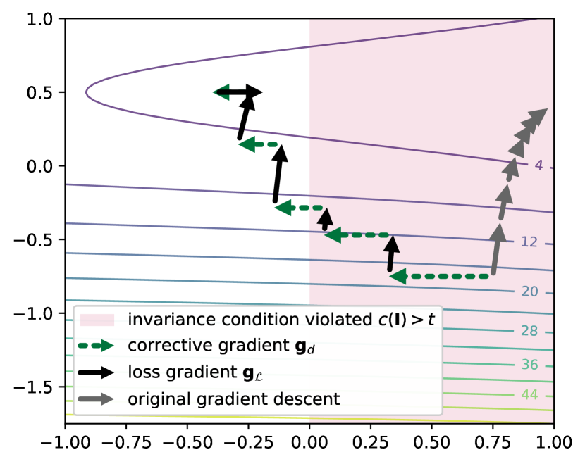
((a))

((b))

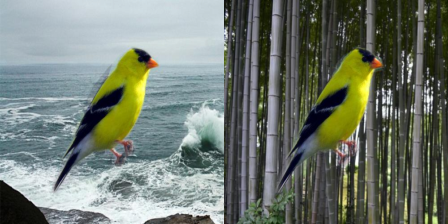
((c))

((d))

Figure 1: Schematic visualization (a) of our optimization approach. The first two loss gradients are scaled to two-thirds the length of the corrective gradient due to the violation of the invariance condition. Invariance pairs for (b) ColoredMNIST, (c) Waterbird-100, and (d) CelebA are used for the invariance condition and corrective gradient formulation.

To effectively generalize to unseen domains or distributions, models should maintain consistent representations across all training environments [3]. Maintaining consistent representations involves identifying and internalizing consistent characteristics from the available sources. Inconsistent characteristics that should not affect the predicted label (such as the color in ColoredMNIST, see Fig. 1(b)), should have no impact on the learned representation. However, if these inconsistent characteristics are poorly represented in the training data, the model may rely on them, if not prevented from doing so [4]. Examples of models relying on such characteristics, resulting in poor performance, include animal detection in unfamiliar environments [5, 6], COVID-19 detection on radiographic images when changing the hospital [7], and the substantial accuracy disparities in gender classification for minority groups, especially regarding skin color [8].

To mitigate such risks, we aim at separating consistent characteristics that define a class from spurious attributes, which are only correlated with the class label in the training data but do not define the class. Inspired by contrastive approaches [9], we define “invariance pairs” as pairs of data points that differ in a single characteristic – e.g., the color – while belonging to the same class – e.g., the digit. Note that the term invariance is sometimes used differently in the field of domain generalization. We denote by invariance the transformations, such as a color change in ColoredMNIST, that do not influence the class (Fig. 1(b)). This notion is in contrast to domain-invariance, which refers to the characteristics of a domain (and typically not a class). We utilize these data pairs to define the desired invariance. The pairs enable us to assess the extent to which the model learned the invariance. If the output of the model varies for such pairs, the model suffers from inconsistency in the representations. The model is considered to have incorporated the invariance when its output remains identical for both elements of the pair.

Although the selection and creation of pairs requires manual effort, Explainable AI (XAI) techniques can assist in identifying candidates. To identify spurious correlations, misclassified samples can be analyzed. XAI methods enable the discovery of counterfactual explanations, i.e., instances that are semantically similar but receive different classifications [10, 11]. Specific techniques exist to generate counterfactual explanations in images [12], as well as more advanced Counterfactual Concept Explanations (CCE) [13]. The user can apply these methods and compare the model’s learned concepts with their mental model and identify spuriously correlated features. Such pairs can expose attributes like skin color [8], animal photo backgrounds [5, 14], or orientation in radiographs [7]. The process helps reveal misconceptions internalized by the model, which are used to derive invariance pairs for our method.

In this work, we introduce Invariance Pair-Guided learning (IPG) that incorporates the invariances during training. In order to guide the neural network, we extend the standard gradient descent-based approach with an additional corrective step, the corrective gradient inspired by van Baelen [15]. The corrective gradient is specified by pairs of input data, the invariance pairs, which define the desired invariance properties of the model. Furthermore, adaptive scaling preserves the corrective effect depending on the extent of invariance internalized by the model. The adaptation is realized by the invariance pairs and an invariance condition, which we introduce, to converge to a generalizable representation. We examine out-of-distribution generalization and robustness of models trained with IPG on three datasets: ColoredMNIST, Waterbird-100, and CelebA. The datasets represent scenarios with strong, including perfect, spurious correlations, either synthetically generated or naturally occurring in real-world data. Fig. 1(a) illustrates how the described corrective gradient helps to avoid a region that violates the invariance condition without any gradient momentum. Our key contributions consist in:

• A novel corrective gradient method (IPG) using invariance pairs with adaptive scaling via an invariance condition to improve out-of-distribution generalization.

• An invariance pair generation approach that extends IPG, i.e., IPG with adversarial augmentation (IPG-AA).

The remainder of the paper is structured as follows. Section 2 discusses related work. In Section 3, we present IPG and IPG-AA. Section 4 evaluates the performance, Section 5 concludes.

2 Related Work

The generalization of machine learning models to unseen distributions has been studied in the fields of robustness [14], domain generalization [2], spurious correlations in machine learning [16, 17], and causality [16]. We categorize related methods into data manipulation, representation learning, and learning strategies, similar to [2, 16]. Our approach integrates representation learning with an adaptive learning strategy.

Data manipulation addresses the problem by either augmenting existing data, generating new data, or adding further information about the underlying concepts. The goal of data augmentation and data generation approaches is to expand the dataset so that the training distribution(s) and the target distribution(s) are closer. For instance, Wang [18] implements augmentation techniques to vary image style, while Prakash [19] embodies synthetic data augmentation to enrich the dataset. Along domain randomization, another method applied in [20, 19], adversarial augmentation [21, 22, 23] is a technique to improve model robustness. Among the adversarial augmentation methods, the DAIR approach reports high performance on ColoredMNIST. The DAIR approach applies regularization based on adversarial augmentation to achieve consistency [21]. Further, a small group of techniques instead aims to provide information about the underlying concepts. For example, methods that complement the estimation with the use of pseudo-labels [24, 25] or concept banks [26, 27]. In addition, a mixup-based technique [28] utilizes class and domain (or group) labels to generate inputs. In Section 4.1, we compare our IPG approach with DAIR. Hereby, we consider two variants of IPG: (a) IPG using adversarial augmentation, and (b) IPG incorporating invariance pairs. In both cases, IPG shows comparable results. Replacing specialized augmentation techniques with invariance pairs improves data efficiency, without needing extra labels for spurious attributes as contained in concept banks.

Representation learning involves feature disentanglement or domain-invariant representation learning. Domain-invariant representation learning uses techniques such as explicit feature alignment [29, 30, 31], domain adversarial learning [32, 33], or Invariant Risk Minimization (IRM) [34]. The main intuition of IRM is to enforce an optimal classifier across all training environments. IRM is particularly interesting when faced with strong spurious correlations, such as those observed in the ColoredMNIST dataset [34]. Further approaches promoting domain-invariant feature learning are EIIL [35] and also SFB [36], which use test-time adaptation. In addition, feature disentanglement is another representation learning strategy that aims to separate spurious and general representations within the latent space. Rao [37] examines an explanation-guided learning approach, which we refer to as EGL. The approach uses a bounding box to formulate a regularization term in the form of an energy pointing game penalizing the attribution of pixels outside the bounding box, i.e., in the background. EGL applies different XAI methods to calculate the attribution: B-cos [38], $\mathcal{X}$-DNN [39], and IxG [40]. Similarly, GALS [41] applies language-guided learning. GALS uses text encodings of an additional text input to also regularize on the attribution of the model. Both approaches are applicable in the presence of perfect spurious correlation. Our approach is founded on the notion of invariance and aims to learn generalizable models by encoding invariance information in the training process. We evaluate our method against IRM-based approaches on the ColoredMNIST dataset and compare it with GALS and EGL on the Waterbird-100 dataset, which has a perfect spurious correlation in the training set. Other representation learning methods are excluded from the comparison as they require multiple training domains or depend on the availability of bias-conflicting groups. We test IPG in these scenarios in Sections 4.1 and 4.2.

Learning strategies can be adopted to achieve robustness and domain generalization. These strategies include ensemble learning [42, 43], meta-learning [44, 45], optimization-based methods [14], and self-supervised learning [46, 47]. Additionally, gradient operation methods [48, 49], among others, have gained prominence. One approach is Shock Graph, which transforms images into shock graphs representing the shape content, thus ignoring color- and texture-based features and associated spurious correlations [50]. Further, self-supervised learning and gradient operation methods can encode invariances during training. Some approaches use contrastive input pairs to promote domain-invariance by pairing similar classes across different domains as positive pairs, and dissimilar classes as negative pairs [46, 51]. Another line of research adopts an ”Identification then Mitigation” strategy to address spurious correlations. Examples include JTT [52] or LfF [43]. JTT identifies misclassified samples, typically bias-conflicting, and up-weights them during a second training phase. Similarly, LfF trains an intentionally biased model to up-weight minority samples when training a second model. Moreover, GroupDRO offers an optimization-based strategy that focuses on minimizing the loss of the worst-performing group [14]. Additionally, Shi [48] proposed a gradient matching scheme for domain generalization by maximizing the inner products of gradients across different domains, aligning gradient directions to promote consistency. Several methods also aim for domain-invariant gradients. One approach regularizes gradients to maintain similarity between original and augmented samples [49]. Fishr [53] applies covariance-based gradient matching across domains, as proposed by Sun [54], to achieve invariant gradients. Methods targeting domain-invariant gradients have shown strong performance on datasets like ColoredMNIST, suggesting their effectiveness when faced with strong spurious correlations. In Section 4.1, we compare our IPG approach with Fishr, JTT, LfF, GroupDRO, and Shock Graph. IPG’s invariance pair formulation does not rely on the support of bias-conflicting groups. Furthermore, its invariance definition goes beyond color- and texture-based information, overcoming the limitations of approaches like Shock Graph.

3 IPG: Invariance Pair-Guided Learning

In this section, we describe our approach to formulating the invariance pairs, the corrective gradient, and the adaptive scaling by the invariance condition.

3.1 Preliminaries and Overview

A training set $\mathcal{D}_{tr}:=\{(\mathbf{x}_{j},y_{j})\}^{n}_{j=1}$ consists of input samples $\mathbf{x}_{j}\in\mathcal{X}$ and labels $y_{j}\in\mathcal{Y}$ of $K$ classes that are distributed according to the joint distribution $P_{\mathcal{D}_{tr}}$. For each data point $\mathbf{x}_{j}$ with class label $y_{j}$, there is a spurious attribute $a_{j}$, where $a_{j}$ is non-predictive of $y_{j}$. Let $\mathcal{A}$ denote the set of all possible spurious attributes. We define a combination of values of $a$ and $y$ as a group $g:=(a,y)\in\mathcal{A}\times\mathcal{Y}$. In $\mathcal{D}_{tr}$, groups are typically imbalanced, so that the co-occurrence of values of $a$ and values of $y$ induces a spurious correlation, denoted as $\langle a,y\rangle$. In extreme cases, which we also consider, a group is completely missing in $\mathcal{D}_{tr}$, resulting in a perfect spurious correlation. A test set $\mathcal{D}_{te}$ shows a different correlation of $a$ and $y$, typically by a reduction or inversion of the correlation. Therefore, the distributions differ $P_{\mathcal{D}_{tr}}\neq P_{\mathcal{D}_{te}}$. Let $P_{\mathcal{D}_{te}^{g}}$ denote the distribution of the test samples of group $g$. Our goal is to learn a generalizable model $f_{\theta}$ independent of $\langle a,y\rangle$ resulting in comparable performance in each group and, accordingly group robustness. Therefore, we investigate the worst-group accuracy $\text{Acc}_{wg}(f_{\theta})$ [55], defined as the minimum accuracy across groups of test samples:

$$\text{Acc}_{wg}(f_{\theta}):=\min_{g\in\mathcal{A}\times\mathcal{Y}}\mathbb{E}_{(x,y)\sim P_{\mathcal{D}_{te}^{g}}}[\mathbf{1}_{y=f_{\theta}(x)}].$$

Our method extends the stochastic mini-batch gradient descent method [56] by incorporating the following key components. First, we introduce a set of invariance pairs, denoted $\mathcal{I}$, describing the invariance that the model should respect. Utilizing $\mathcal{I}$ and batches $\mathbf{I}$ sampled from $\mathcal{I}$, we derive a corrective gradient, referred to as $\mathbf{g}_{d}$, that is applied before each gradient step. Finally, we use an invariance condition $c(\mathbf{I})$ to adaptively scale the loss gradient. An overview is given in Fig. 2. We detail each of those components in the following.

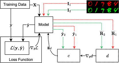
Figure 2: Schematic overview of the IPG training method (dotted) as an extension to the traditional approach using the example of ColoredMNIST.

3.2 Rationale and Invariance Pair Definition

To compare the learned characteristics and formulate a corrective gradient $\mathbf{g}_{d}$, we use a form of latent representation, a rationale matrix. The rationale, as proposed by Chen [31], represents the concepts learned by the model. To this end, a neural network used for classification is divided into two parts. First, we have the feature extractor $f$, consisting of the first up to the last hidden layer, which maps inputs $\mathbf{x}$ to features $\mathbf{z}:=f(\mathbf{x})$. Second, the classifier $h$ maps $\mathbf{z}$ to logits $\mathbf{o}$, defined as $\mathbf{o}:=h(\mathbf{z})$. The rationale $\mathbf{R}$ connects $\mathbf{z}$ and the weights of $h$. The matrix $\mathbf{R}$ represents the concepts that the neural network has learned from the training data in an accessible way [31]. Specifically, we define the rationale as a matrix consisting of the products of the weights $\mathbf{W}_{i,j}$ of $h$ and their corresponding feature $z_{i}$:

$$\mathbf{R}:=\begin{bmatrix}\mathbf{W}_{\{1,1\}}z_{1}&\mathbf{W}_{\{1,2\}}z_{1}&\dots&\mathbf{W}_{\{1,K\}}z_{1}\\ \mathbf{W}_{\{2,1\}}z_{2}&\mathbf{W}_{\{2,2\}}z_{2}&\dots&\mathbf{W}_{\{2,K\}}z_{2}\\ \vdots&\vdots&\ddots&\vdots\\ \mathbf{W}_{\{D,1\}}z_{D}&\mathbf{W}_{\{D,2\}}z_{D}&\dots&\mathbf{W}_{\{D,K\}}z_{D}\\ \end{bmatrix}.$$

We use the subscripts to indicate that $\mathbf{R}_{\mathbf{x}}$ was generated by inference on the input $\mathbf{x}$. The number of the features $D$ and the number of the classes $K$ determine the shape of the matrix $\mathbf{R}\in\mathbb{R}^{D\times K}$. The outputs of the neural network $\mathbf{\hat{y}}$ are defined by applying the softmax function to the logits, $\mathbf{\hat{y}}:=softmax(\mathbf{o})$. We select $\mathbf{R}$ for our method because it is fine-grained and incorporates the weights of the final layer. We use the rationale matrix to compare the learned characteristics of the input to guide the model during the training process.

To identify undesired learned concepts, we contrast rationale matrices derived from invariant input pairs. We use a set $\mathcal{I}$ of invariant pairs $(\mathbf{x}_{1},\mathbf{x}_{2})\in\mathcal{I}$ to define a specific invariance. Each pair $(\mathbf{x}_{1},\mathbf{x}_{2})$ consists of elements contrasting a difference that should be invariant to the final classification. Although $\mathbf{x}_{1}$ and $\mathbf{x}_{2}$ are different, the defined characteristic should not affect the classification result. For example, the ColoredMNIST dataset consists of colored digits, with color serving as the spurious attribute. Therefore, $\mathbf{x}_{1}$ and $\mathbf{x}_{2}$ represent the same digit in different colors (Fig. 1(b)). These input pairs are either generated by augmentation or manually selected, e.g., based on CCE [13]. Multiple pairs are used to describe one invariance. In each training step, we randomly sample a batch of invariance pairs $\mathbf{I}$ from $\mathcal{I}$ with replacement using the same batch size as for the training data. We refer to the set of all the first elements of the invariance pairs as $\mathcal{I}_{1}$ and all second elements as $\mathcal{I}_{2}$. Similarly, we apply the notation for $\mathbf{I}_{1}$ and $\mathbf{I}_{2}$. These pairs define the invariance that the model should internalize during the learning process based on rationales.

We also consider IPG with adversarial augmentation (IPG-AA), which replaces $\mathbf{I}$ with pairs generated for the current data batch. Specifically, for each input batch, we generate a corresponding set of $\mathbf{I}$ based on the input batch. The set $\mathbf{I}$ is generated following the original methodology, except that $\mathbf{I}$ is updated for each step.

3.3 Corrective Gradient and Invariance Condition

We combine the rationales of the invariance pairs to formulate a distance measure. With this measure, we quantify the level of internalization of the specified invariance. As we have multiple pairs describing one invariance, we have multiple rationales for each element in those pairs. In order to achieve one representation of the rationales for $\mathbf{I}_{1}$, we calculate a mean rationale:

$$\mathbf{\overline{R}}_{1}:=\frac{1}{|\mathbf{I}_{1}|}\sum_{\mathbf{x}\in\mathbf{I}_{1}}\mathbf{R}_{\mathbf{x}}.$$

In this mean rationale $\mathbf{\overline{R}}_{1}$, shared concepts in all data points in $\mathbf{I}_{1}$ are aggregated, whereby rationales that are only local in data points vanish. We calculate $\mathbf{\overline{R}}_{2}$ analogously. Note that we expect ordered pairs such that the elements in $\mathbf{I}_{1}$ share the same characteristic, which should be invariant to the shared characteristic of the elements in $\mathbf{I}_{2}$. For example, in the case of ColoredMNIST, all elements in $\mathbf{I}_{1}$ are red, while all elements in $\mathbf{I}_{2}$ are green. Since pairs are invariant by definition, $\mathbf{\overline{R}}_{1}$ and $\mathbf{\overline{R}}_{2}$ should be similar to encode this invariance. To verify the learning of this invariance, we formulate a distance measure:

$$d(\mathbf{I}):=||\mathbf{\overline{R}}_{1}-\mathbf{\overline{R}}_{2}||_{2}.$$

The distance $d(\mathbf{I})$ is induced by the spectral norm. Therefore, $d(\mathbf{I})$ refers to the largest singular value of the difference in mean rationales, capturing the most prominent characteristic. Based on the distance in rationales, we can encode the invariance.

To guide the neural network towards robust representations during the training process, we use the distance measure $d(\mathbf{I})$ to incorporate the invariance information. To this end, we extend the mini-batch gradient descent by introducing a two-step update mechanism. As a first step, we perform a correction step based on the instances in $\mathbf{I}$. We update the weights $\mathbf{\theta}$ of the model according to the gradient of the rationale distance $\mathbf{g}_{d}:=\nabla_{\mathbf{\theta}}d(\mathbf{I})$ using a weight update function $\sigma$. The step $\mathbf{g}_{d}$ aims to minimize the distance between different elements in $\mathbf{I}$. As a second step, we update the weights $\mathbf{\theta}$ of the model based on $\nabla_{\mathbf{\theta}}\mathcal{L}$. However, the compatibility of both updates must be maintained to preserve a corrective effect of $\mathbf{g}_{d}$. For this reason, $\nabla_{\mathbf{\theta}}\mathcal{L}$ is scaled adaptively. We scale according to length of the gradient measured by the Euclidean norm or $\ell_{2}$ norm. The length of $\nabla_{\mathbf{\theta}}\mathcal{L}$ is adjusted based on an invariance condition and the length of $\mathbf{g}_{d}$. To this end, we introduce an invariance condition by a symmetric version of the Kullback-Leibler (KL) divergence between the model outputs $\tilde{\textbf{y}}_{1}$ and $\tilde{\textbf{y}}_{2}$ of $\mathbf{I}_{1}$ and $\mathbf{I}_{2}$, respectively:

$$c(\mathbf{I}):=\frac{1}{2}\big{(}KL(\tilde{\textbf{y}}_{1}||\tilde{\textbf{y}}_{2})+KL(\tilde{\textbf{y}}_{2}||\tilde{\textbf{y}}_{1})\big{)}.$$

A violation occurs when $c(\mathbf{I})$ exceeds a predefined threshold $t$. In order to adjust the influence of the gradients, we define the rescaling function:

$$s(\mathbf{g}_{1},\mathbf{g}_{2}):=\frac{\mathbf{g}_{1}}{||\mathbf{g}_{1}||_{2}}\max\{\varepsilon,||\mathbf{g}_{2}||_{2}\},$$

which scales a vector $\mathbf{g}_{1}$ to the length of $\mathbf{g}_{2}$ based on the Euclidean norm or a minimum length of $\varepsilon$ [15]. In case of a violation ($c(\mathbf{I})>t$), we scale $\nabla_{\mathbf{\theta}}\mathcal{L}$ to a fraction $\alpha\in\left[0,1\right]$ of the length of $\mathbf{g}_{d}$ or $\varepsilon$. Otherwise, we apply $\nabla_{\mathbf{\theta}}\mathcal{L}$, whereas the vector length is limited by twice the length of $\mathbf{g}_{d}$:

$$\mathbf{g}_{\mathcal{L}}:=\begin{cases}\alpha\cdot s(\nabla_{\mathbf{\theta}}\mathcal{L},\mathbf{g}_{d})&\textbf{if }c(\mathbf{I})>t\\[4.30554pt] \underset{\mathbf{g}\in\big{\{}\nabla_{\mathbf{\theta}}\mathcal{L},s(\nabla_{\mathbf{\theta}}\mathcal{L},2\cdot\mathbf{g}_{d})\big{\}}}{\arg\min}||\mathbf{g}||_{2}&\textbf{else}\end{cases}.$$ (1)

Eq. 1 rescales $\nabla_{\mathbf{\theta}}\mathcal{L}$ based on the length determined by the Euclidean norm of $\mathbf{g}_{\mathcal{L}}$ (or a minimum value of $\varepsilon$), when the invariance condition is violated. The rescaling of the corrective gradient based on the invariance condition allows for an adaptive regulation of the learned invariance, when necessary. In addition, the length of $\mathbf{g}_{\mathcal{L}}$ is limited to a maximum length of $2\cdot||\mathbf{g}_{d}||_{2}$ to homogenize the gradient-magnitude in regions where $2\cdot||\mathbf{g}_{d}||_{2}<||\nabla_{\mathbf{\theta}}\mathcal{L}||_{2}$. In such regions, the corrective effect may be undermined, as convergence to a subspace satisfying the invariance condition may result in a sudden large step. For both updates, the same learning rate $\eta$ is used. We apply a KL divergence of the outputs as an invariance condition as it is more sensitive than defining a threshold on $d(\mathbf{I})$. Therefore, correction is applied earlier when the model tends to rely on invariant features. In addition, the training process is less constrained when the invariance condition is met. We update the weights using the optimization function $\sigma$ that can involve momentum-based techniques allowing for a stabilizing effect. The additional corrective update step via $\mathbf{g}_{d}$ reduces $d(\mathbf{I})$, corrects the overall rationale, and thus encodes the invariance.

An overview of the presented method is shown in Alg. 1 defining the extended update function for one gradient descent step for a training-data batch given by $(\mathbf{X},\mathbf{y})$.

Algorithm 1 IPG update step

1:$\mathbf{\theta}$, $\mathbf{X}$, $\mathbf{y}$, $\mathbf{I}$, $\alpha$, $\eta$, $t$, $\varepsilon$

2:for $i\in\{1,2\}$ do $\triangleright$ calculate distance measure $d$

3:  $\mathbf{z}_{i}\leftarrow f(\mathbf{I}_{i};\mathbf{\theta}_{f})$

4:  for $k\in\{1,2\}$ do

5:   $\mathbf{R}_{i,k}\leftarrow\mathbf{\theta}_{h,k}\cdot\mathbf{z}_{i}$

6:  end for

7:  $\mathbf{\overline{R}}_{i,k,c}\leftarrow\frac{1}{N}\sum^{N}_{n=1}\mathbf{R}_{i,k,c,n}$

8:  $\tilde{\textbf{y}}_{i}\leftarrow softmax(h(\mathbf{z}_{i};\mathbf{\theta}_{h}))$

9:end for

10:$d\leftarrow||\mathbf{\overline{R}}_{1}-\mathbf{\overline{R}}_{2}||_{2}$

11:$\mathbf{g}_{d}\leftarrow\nabla_{\mathbf{\theta}}d$ $\triangleright$ calculate corrective gradient

12:$\mathbf{\theta}\leftarrow\sigma(\mathbf{\theta},\eta,\mathbf{g}_{d})$ $\triangleright$ update weights

13:$\hat{\mathbf{y}}\leftarrow softmax(h(f(\mathbf{x};\mathbf{\theta}_{f});\mathbf{\theta}_{h}))$ $\triangleright$ classify

14:$\mathbf{g}_{\mathcal{L}}\leftarrow\nabla_{\mathbf{\theta}}\mathcal{L}(\mathbf{y},\hat{\mathbf{y}})$ $\triangleright$ calculate loss gradient

15:$c\leftarrow\frac{1}{2}(KL(\tilde{\textbf{y}}_{1}||\tilde{\textbf{y}}_{2})+KL(\tilde{\textbf{y}}_{2}||\tilde{\textbf{y}}_{1}))$ $\triangleright$ scale $\mathbf{g}_{\mathcal{L}}$ on invariance condition violation

16:if $c>t$ then

17:  $\mathbf{g}_{\mathcal{L}}\leftarrow\alpha\cdot\frac{\mathbf{g}_{\mathcal{L}}}{||\mathbf{g}_{\mathcal{L}}||_{2}}\max\{\varepsilon,||\mathbf{g}_{d}||_{2}\}$

18:else

19:  if $||\mathbf{g}_{\mathcal{L}}||_{2}>2\cdot\max\{\varepsilon,||\mathbf{g}_{d}||_{2}\}$ then

20:   $\mathbf{g}_{\mathcal{L}}\leftarrow 2\cdot\frac{\mathbf{g}_{\mathcal{L}}}{||\mathbf{g}_{\mathcal{L}}||_{2}}\max\{\varepsilon,||\mathbf{g}_{d}||_{2}\}$

21:  end if

22:end if

23:$\mathbf{\theta}\leftarrow\sigma(\mathbf{\theta},\eta,\mathbf{g}_{\mathcal{L}})$ $\triangleright$ update weights

4 Experiments

In this section, we present the evaluation method and the results.

We evaluate IPG using the following three datasets: ColoredMNIST [34], Waterbird-100 [41], and CelebA [14]. These datasets exhibit a strong binary spurious correlation attribute. The attributes are color (red or green), background (water or land), and gender (female or male) for the ColoredMNIST, Waterbird-100, and CelebA datasets, respectively. The classes are binary in each dataset: In ColoredMNIST, they consist of digit groups 0-4 and 5-9. In Waterbird-100, the classes are waterbird and landbird. In CelebA, they are blond and non-blond hair. ColoredMNIST is structured as a domain generalization dataset, while Waterbird-100 and CelebA are motivated by group robustness. Therefore, ColoredMNIST is evaluated on a test dataset, where the spurious correlation is opposite to the training dataset, representing an out-of-distribution domain. ColoredMNIST has a label noise of $25\%$. Waterbird-100, and CelebA are typically evaluated based on the entire test dataset, focusing on the worst-group accuracy to measure group robustness. Waterbird-100 is a special case, where the training dataset contains only perfectly correlated pairs. For this dataset, we also test the reversed setting, predicting the background as a label instead of the bird type.

In order to guide the gradient in the learning phase, we select a set of invariance pairs, denoted as $\mathcal{I}$. These pairs are crucial as they define the specific invariance that the model is expected to learn. Specifically, for the ColoredMNIST dataset, we choose pairs of different colors, as illustrated in Fig. 1(b). For the Waterbird-100 dataset, we use pairs with the same bird but backgrounds from different environments (Fig. 1(c)). The complementary image in each pair is created by flipping the color of the original image in ColoredMNIST. For the Waterbird-100 dataset, we generate a pair by exchanging the background randomly with one of the other type. For the reversed version, we substitute the bird in a similar way. For CelebA, we apply a GAN-based latent space modification, to generate a gender-swapped version of a given CelebA-HQ image [57]. We order the generated images by the Mahalobis distance [58] of the latent representation of a trained ERM model to other female (or male) images in the training dataset and manually select the images (Fig. 1(d)).

We train the models with the following specifications. The model architecture for experiments based on ColoredMNIST is a convolutional neural network and follows the DomainBed framework [59], commonly used for benchmarking. For Waterbird-100 and CelebA, we use a ResNet-50 [60]. Accuracy is evaluated over $10$ trials, with different model initializations. Model selection is based on the highest mean validation accuracy for ColoredMNIST and maximum worst-case validation accuracy for Waterbird-100 and CelebA. The hyperparameters (Tab. 1) are selected using the Tree-structured Parzen Estimator with $100$ trials per dataset [61]. This setup supports our accuracy comparison and latent representation analysis.

Table 1: Hyper-parameter configuration of IPG in experiments.

Dataset	Model	$\alpha$	$t$	$|\mathcal{I}|$	$\eta$	Batch Size	Nr. Epochs
ColoredMNIST	IPG, IPG-AA	$110-1$	$210-6$	$300$	$110-3$	128	18
Waterbird-100	IPG	$510-1$	$210-4$	$300$	$110-4$	32	10
CelebA	IPG	$110-2$	$110-4$	$271$	$110-3$	128	10
CelebA	GroupDRO+IPG	$8510-2$	$110-1$	$271$	$110-3$	128	10

4.1 Accuracy Comparison

ColoredMNIST: For ColoredMNIST, we examine IPG based on the accuracy on the test dataset. In this dataset, the correlation of color and label inverses relative to the samples observed during the training phase. Our approach achieves a mean test accuracy of $72.7\%$. Due to the inherent labeling noise in the dataset, the theoretical maximum accuracy is limited to $75\%$ [34]. Tab. 2(a) shows an overview of the accuracy and the standard error for the test dataset compared to state of the art approaches. It should be noted that the performance comparison may not be entirely fair, as both the IRM approaches as well as the Fishr method lack access to external information, such as $\mathcal{I}$, which IPG uses [53, 62, 34]. Further, the Shock Graph approach derives a shape-based representation of the digit and therefore removes the color information [50]. We argue that the transformation serves as a method for encoding dataset-specific knowledge about invariant representations. Additionally, we also list an Empirical Risk Minimization (ERM) approach as a baseline and another ERM-based approach learning on grayscale images, serving as an oracle [34]. IPG shows the highest mean accuracy compared to other methods, benefiting from the explicit incorporation of invariances provided by $\mathcal{I}$.

Table 2: Accuracy comparison on ColoredMNIST without (a) and with (b) adversarial or random augmentation.

((a))

Approach	Accuracy
ERM	$16.1\pm 0.8$
IRM [34]	$66.9\pm 2.5$
meta-IRM [62]	$70.4\pm 0.9$
Fishr [53]	$68.8\pm 1.4$
Shock Graph [50]	$71.6$
IPG (ours)	$\mathbf{72.7\pm 0.3}$
Random	$50.0\pm 0.0$
ERM grayscale (oracle)	$73.1\pm 0.4$
Optimal	$75.0\pm 0.0$

((b))

Approach	Accuracy
DAIR-AA [21]	$72.6\pm 0.1$
DAIR-RA [21]	$73.1\pm 0.1$
IPG-AA (ours)	$\mathbf{73.3\pm 0.4}$
Random	$50.0\pm 0.0$
ERM grayscale (oracle)	$73.1\pm 0.4$
Optimal	$75.0\pm 0.0$

As an additional performance comparison, we examine DAIR by using adversarial augmentation. DAIR encodes augmented inputs in the loss function. Both, the original and the augmented input are processed by the neural network in a feed-forward step. In this way, the spurious correlation is effectively mitigated within the ColoredMNIST dataset. For comparison, we extend our IPG approach with adversarial augmentation, i.e., IPG-AA, representing perfect invariance information. We then compare IPG-AA with two variants of DAIR: one that uses adversarial augmentation (DAIR-AA) and another using random augmentation (DAIR-RA) [21]. The accuracy on the test environment is shown in Tab. 2(b). We conclude that IPG-AA achieves a higher mean test accuracy than DAIR-based approaches or the ERM-grayscale approach. Summarizing, IPG and IPG-AA reach state of the art results in both test scenarios.

Waterbird-100: We further evaluate the performance of IPG on the Waterbird-100 dataset, which has a perfect spurious correlation in the training set: every waterbird image has a water background, while every landbird image shows land or forest. Additionally, multiple bird species represent each class, making it more complex to learn the defining characteristics of the birds compared to the simpler background features. The test dataset includes instances from all groups, with a particular focus on the worst-group accuracy. We also examine a reversed setting, where labels and spurious attributes are swapped, following prior studies by Rao [37] and Petryk [41]. Unlike the digits in ColoredMNIST, birds show more complex patterns, there is only one training domain, and the training dataset lacks bias-conflicting samples. We compare our approach to the explanation-guided learning method, which we refer to as EGL [37], and the language-guided learning method GALS [41]. EGL applies different XAI methods: B-cos [38], $\mathcal{X}$-DNN [39], and IxG [40], to calculate feature attributions. Additionally, we apply an ERM based approach as baseline. Tab. 3 summarizes the results. ERM achieves the highest overall accuracy for both Waterbird-100 versions, mainly at the expense of the minority classes. IPG achieves higher worst-group accuracy compared to GALS, EGL, and ERM. These findings indicate that invariance-pair guidance effectively encodes the desired invariance. We conclude that IPG achieves higher worst-group accuracy compared to the baselines on both versions of the Waterbird-100 dataset, representing a state of the art result to the best of our knowledge.

Table 3: Accuracy comparison on Waterbird-100 and Waterbird-100-reverse.

	Waterbird-100		Waterbird-100-reverse
Model	Overall Acc. ↑	$\text{Acc}_{wg}$ ↑	Overall Acc. ↑	$\text{Acc}_{wg}$ ↑
EGL B-cos [37]	$71.1\pm 0.9$	$41.0\pm 2.1$	$83.6\pm 1.1$	$62.8\pm 2.1$
EGL $\mathcal{X}$-DNN [37]	$73.1\pm 3.4$	$47.0\pm 9.1$	$82.6\pm 2.0$	$63.9\pm 3.6$
EGL IxG [37]	$78.1\pm 2.6$	$56.1\pm 7.0$	$78.9\pm 1.9$	$56.5\pm 3.7$
GALS [41]	$79.7$	$56.7$	$86.8$	$72.9$
ERM	$\mathbf{99.4\pm 0.1}$	$37.2\pm 0.2$	$\mathbf{99.4\pm 0.1}$	$56.6\pm 2.4$
IPG (ours)	$85.92\pm 2.29$	$\mathbf{68.62\pm 3.37}$	$92.13\pm 1.03$	$\mathbf{84.53\pm 2.63}$

CelebA: Finally, we evaluate the performance of our approach on the CelebA dataset, which exhibits gender as a spurious attribute. Compared to ColoredMNIST and Waterbird-100, the formulation of pairs is more challenging, since the spurious attribute is not synthetic. We use the image-to-image translation technique [57] to generate pairs. IPG is compared to several established methods. We evaluate GroupDRO [14], a technique that uses group information during training, along with a combined approach integrating both IPG and GroupDRO. Additionally, we evaluate JTT [52] and LfF [43], which operate without requiring additional information, relying instead on intentionally biased models. We also examine ERM as a baseline approach without guidance. Our findings reveal that ERM achieves the highest overall accuracy. The worst-case accuracy of IPG alone ($73.2\%$) is lower than that of JTT or GroupDRO. However, when combined with GroupDRO, IPG achieves slightly higher worst-case accuracy and exhibits reduced variance compared to GroupDRO alone. In general, the corrective gradient introduced by IPG helps to improve worst-case performance, as shown by its superior worst-case accuracy compared to ERM. Nonetheless, JTT achieves higher worst-case accuracy than IPG without the need for additional information. Tab. 4 summarizes the results and compares requirements for additional group labels or pairs. A notable challenge in using IPG lies in the definition of effective pairs, which is crucial for maintaining compatibility with the dataset domain. The applied image-to-image translation technique, for instance, can produce outputs that deviate in unwanted characteristics from the original image domain, such as generating blonder hair for women (Fig. 1(d)). The results indicate that while IPG enhances worst-case performance, it still falls short of the state of the art results achieved by GroupDRO or JTT, primarily due to difficulties in defining effective pairs.

Table 4: Accuracy comparison on CelebA.

Model	Additional Info	Overall Acc. ↑	$\text{Acc}_{wg}$ ↑
GroupDRO [14]	$g$	$92.9\pm 0.2$	$88.9\pm 2.3$
JTT [52]	-	$88.0$	$81.1$
LfF [43]	-	$86.0$	$70.6$
ERM	-	$\mathbf{94.9\pm 0.2}$	$47.8\pm 3.7$
IPG (ours)	$\mathcal{I}$	$89.9\pm 3.2$	$73.2\pm 7.5$
GroupDRO+IPG (ours)	$\mathcal{I}$, $g$	$92.3\pm 0.3$	$\mathbf{89.6\pm 1.3}$

4.2 Latent Representation Analysis

We inspect the latent representation of models trained with IPG and ERM, focusing on their ability to learn the invariance. To analyze and compare the internal representation of the neural network, we trained two different models. A model $M_{IPG}$ is trained with IPG encoding the invariance, while a model $M_{ERM}$ is trained with ERM without explicit invariance information. For both trained models, we compute the rationale $\mathbf{R}_{\mathbf{x}}$ from an input $\mathbf{x}$ for random samples of the test sets of ColoredMNIST, Waterbird-100, and CelebA. Then, to reduce the dimension of the rationale to two, t-SNE [63] is applied to the (vectorized) rationales $\mathbf{R}_{\mathbf{x}}$ with a perplexity of $200$. The resulting illustration, as shown in Fig. 3, exhibits differences in the latent representation. Since all instances represent the same class, they are ideally represented in one cluster without separation based on the spurious attribute. Especially for ColoredMNIST, a clear separation based on the spurious attribute color for $M_{ERM}$ is visible as of the inherent label noise. In contrast, for $M_{IPG}$, the model shows a mixture of red and green instances without a clear color-based separation. For the Waterbird-100 and CelebA results, we find a higher overlap of instances differing in spurious attributes for $M_{IPG}$, while $M_{ERM}$ shows a clearer separation of these instances. Thus, the rationales of $M_{IPG}$ seem to better reflect the underlying structure associated with $y$, in contrast to the rationales of $M_{ERM}$, which appear to be more influenced by the spurious attribute. Fig. 3 depicts the representations for a single class, but similar characteristics are observed for all classes. From these observations, we conclude that the latent representation of $M_{IPG}$ shows visible signs of internalized invariance through the invariance correction of IPG.

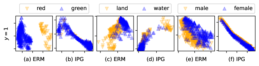
Figure 3: Visualization of the rationales for $y=1$ of an ERM- and an IPG-based approach for ColoredMNIST (a-b), Waterbird-100 (c-d), and CelebA (e-f).

4.3 Discussion and Limitations

In the previous experiments, we examined the characteristics of IPG. We found that IPG and IPG-AA reach state of the art performance on ColoredMNIST (Tab. 2(a) and 2(b)). We showed that IPG outperforms current approaches on the Waterbird-100 dataset and its reversed version (Tab. 3), which is particularly challenging because of its inherent perfect spurious correlation. We also found that IPG can improve performance on the real-world dataset CelebA without the need for the group labels (Tab. 4). However, there are efficient methods, such as JTT that perform better. Only when combined with GroupDRO, IPG can reach state of the art results. For real-world datasets, the explicit pair formulation might be interesting, whereas the implicit formulation, as in JTT, is imprecise. In addition, we have shown that the resistance to the inherent spurious correlation comes along with well-represented latents (Fig. 3). These results show that the proposed approach effectively encodes invariance in the presence of significant spurious correlation.

Despite the successful encoding of invariance, some limitations still need to be addressed. First, the invariance condition and the corrective gradient based on rationale matrices are associated with a task outputting logits, such as classification. Using other tasks, such as regression, is worth investigating. Second, the computational complexity is increased primarily due to the additional pair calculation of $2|\mathcal{I}|$ inference steps and the corrective gradient step. Future work could investigate, whether corrective gradients can be omitted in certain steps. Third, the results on CelebA indicate that the method is highly dependent on the quality of invariance pairs. Future work could explore ways to ensure quality. In addition, while image-to-image translation techniques can help to produce the pairs, they can also suffer from bias, which needs to be mitigated by manual inspection. Finally, we plan to extend to multiple invariances, e.g., by combining the correction gradients, e.g., by averaging or addition.

5 Conclusion

This work proposes a novel method to define and learn invariance through the IPG approach, which allows to specify invariance pairs. Based on the pairs, we define an invariance condition and a corrective gradient. These components allow for an adaptive regulation of the training phase of the neural network. In this way, invariance is encoded while maintaining the flexibility of the models. With IPG, spurious correlations can be compensated to improve the out-of-distribution performance and thus make the models more robust. IPG (i) operates on a single domain, (ii) utilizes data-efficient pair formulation without requiring specialized augmentation, (iii) applies to datasets without bias-conflicting groups, and (iv) eliminates the need for pre-processing of the dataset. We validated the effectiveness of IPG on the ColoredMNIST, the Waterbirds-100(-reversed), and the CelebA datasets. For Waterbirds-100, IPG demonstrated a notable improvement of $11.91$ percentage points in mean worst-case accuracy. On the real-world CelebA dataset, IPG is limited by pair quality, however, IPG proved beneficial when combined with GroupDRO. In the future, we plan to apply IPG to datasets with multiple invariances.

References

- \bibcommenthead
- Kohli and Chadha [2020] Kohli, P., Chadha, A.: Enabling pedestrian safety using computer vision techniques: A case study of the 2018 Uber inc. self-driving car crash. In: Advances in Information and Communication, pp. 261–279 (2020)
- Wang et al. [2023] Wang, J., Lan, C., Liu, C., Ouyang, Y., Qin, T., Lu, W., Chen, Y., Zeng, W., Yu, P.S.: Generalizing to unseen domains: A survey on domain generalization. IEEE Transactions on Knowledge and Data Engineering 35(8), 8052–8072 (2023)
- Ben-David et al. [2006] Ben-David, S., Blitzer, J., Crammer, K., Pereira, F.: Analysis of representations for domain adaptation. In: Advances in Neural Information Processing Systems, vol. 19 (2006)
- Wimmer et al. [2025] Wimmer, L., Bischl, B., Bothmann, L.: Trust me, I know the way: Predictive uncertainty in the presence of shortcut learning. ArXiv preprint arXiv:2502.09137 (2025)
- Beery et al. [2018] Beery, S., Horn, G.V., Perona, P.: Recognition in terra incognita. In: European Conference on Computer Vision, pp. 456–473 (2018)
- Bothmann et al. [2023] Bothmann, L., Wimmer, L., Charrakh, O., Weber, T., Edelhoff, H., Peters, W., Nguyen, H., Benjamin, C., Menzel, A.: Automated wildlife image classification: An active learning tool for ecological applications. Ecological Informatics 77, 102231 (2023)
- DeGrave et al. [2021] DeGrave, A.J., Janizek, J.D., Lee, S.-I.: AI for radiographic covid-19 detection selects shortcuts over signal. Nature Machine Intelligence 3(7), 610–619 (2021)
- Buolamwini and Gebru [2018] Buolamwini, J., Gebru, T.: Gender shades: Intersectional accuracy disparities in commercial gender classification. In: Conference on Fairness, Accountability and Transparency, pp. 77–91 (2018)
- Le-Khac et al. [2020] Le-Khac, P.H., Healy, G., Smeaton, A.F.: Contrastive representation learning: A framework and review. IEEE Access 8, 193907–193934 (2020)
- Wachter et al. [2017] Wachter, S., Mittelstadt, B., Russell, C.: Counterfactual explanations without opening the black box: Automated decisions and the GDPR. Harvard Journal of Law & Technology 31, 841 (2017)
- Dandl et al. [2020] Dandl, S., Molnar, C., Binder, M., Bischl, B.: Multi-objective counterfactual explanations. In: International Conference on Parallel Problem Solving from Nature, pp. 448–469 (2020)
- Goyal et al. [2019] Goyal, Y., Wu, Z., Ernst, J., Batra, D., Parikh, D., Lee, S.: Counterfactual visual explanations. In: International Conference on Machine Learning, pp. 2376–2384 (2019)
- Abid et al. [2022] Abid, A., Yuksekgonul, M., Zou, J.: Meaningfully debugging model mistakes using conceptual counterfactual explanations. In: International Conference on Machine Learning, pp. 66–88 (2022)
- Sagawa et al. [2020] Sagawa, S., Koh, P.W., Hashimoto, T.B., Liang, P.: Distributionally robust neural networks for group shifts: On the importance of regularization for worst-case generalization. In: International Conference on Learning Representations (2020)
- Van Baelen and Karsmakers [2022] Van Baelen, Q., Karsmakers, P.: Constraint guided gradient descent: Guided training with inequality constraints. In: European Symposium on Artificial Neural Networks, Computational Intelligence and Machine Learning, pp. 175–180 (2022)
- Ye et al. [2024] Ye, W., Zheng, G., Cao, X., Ma, Y., Zhang, A.: Spurious correlations in machine learning: A survey. ArXiv preprint arXiv:2402.12715 (2024)
- Steinmann et al. [2024] Steinmann, D., Divo, F., Kraus, M., Wüst, A., Struppek, L., Friedrich, F., Kersting, K.: Navigating shortcuts, spurious correlations, and confounders: From origins via detection to mitigation. ArXiv preprint arXiv:2412.05152 (2024)
- Wang et al. [2021] Wang, Z., Luo, Y., Qiu, R., Huang, Z., Baktashmotlagh, M.: Learning to diversify for single domain generalization. In: IEEE/CVF International Conference on Computer Vision, pp. 834–843 (2021)
- Prakash et al. [2019] Prakash, A., Boochoon, S., Brophy, M., Acuna, D., Cameracci, E., State, G., Shapira, O., Birchfield, S.: Structured domain randomization: Bridging the reality gap by context-aware synthetic data. In: IEEE International Conference on Robotics and Automation, pp. 7249–7255 (2019)
- Yue et al. [2019] Yue, X., Zhang, Y., Zhao, S., Sangiovanni-Vincentelli, A., Keutzer, K., Gong, B.: Domain randomization and pyramid consistency: Simulation-to-real generalization without accessing target domain data. In: IEEE/CVF International Conference on Computer Vision, pp. 2100–2110 (2019)
- Huang et al. [2023] Huang, T., Halbe, S.A., Sankar, C., Amini, P., Kottur, S., Geramifard, A., Razaviyayn, M., Beirami, A.: Robustness through data augmentation loss consistency. Transactions on Machine Learning Research (2023)
- von Kügelgen et al. [2021] Kügelgen, J., Sharma, Y., Gresele, L., Brendel, W., Schölkopf, B., Besserve, M., Locatello, F.: Self-supervised learning with data augmentations provably isolates content from style. In: Advances in Neural Information Processing Systems, vol. 34, pp. 16451–16467 (2021)
- Puli et al. [2024] Puli, A., Joshi, N., Wald, Y., He, H., Ranganath, R.: Nuisances via negativa: Adjusting for spurious correlations via data augmentation. Transactions on Machine Learning (2024)
- Nam et al. [2022] Nam, J., Kim, J., Lee, J., Shin, J.: Spread spurious attribute: Improving worst-group accuracy with spurious attribute estimation. In: Conference on Learning Representations (2022)
- Srivastava et al. [2020] Srivastava, M., Hashimoto, T., Liang, P.: Robustness to spurious correlations via human annotations. In: International Conference on Machine Learning, pp. 9109–9119 (2020)
- Wu et al. [2023] Wu, S., Yuksekgonul, M., Zhang, L., Zou, J.: Discover and cure: Concept-aware mitigation of spurious correlation. In: International Conference on Machine Learning, pp. 37765–37786 (2023)
- Koh et al. [2020] Koh, P.W., Nguyen, T., Tang, Y.S., Mussmann, S., Pierson, E., Kim, B., Liang, P.: Concept bottleneck models. In: International Conference on Machine Learning, pp. 5338–5348 (2020)
- Yao et al. [2022] Yao, H., Wang, Y., Li, S., Zhang, L., Liang, W., Zou, J., Finn, C.: Improving out-of-distribution robustness via selective augmentation. In: International Conference on Machine Learning (2022)
- Jin et al. [2022] Jin, X., Lan, C., Zeng, W., Chen, Z.: Style normalization and restitution for domain generalization and adaptation. IEEE Transactions on Multimedia 24, 3636–3651 (2022)
- Fan et al. [2021] Fan, X., Wang, Q., Ke, J., Yang, F., Gong, B., Zhou, M.: Adversarially adaptive normalization for single domain generalization. In: IEEE/CVF Conference on Computer Vision and Pattern Recognition, pp. 8204–8213 (2021)
- Chen et al. [2023] Chen, L., Zhang, Y., Song, Y., Hengel, A., Liu, L.: Domain generalization via rationale invariance. In: IEEE/CVF Conference on Computer Vision and Pattern Recognition, pp. 1751–1760 (2023)
- Luo et al. [2021] Luo, J., Guo, J., Qiu, W., Huang, Z., Hui, H.: Scale invariant domain generalization image recapture detection. In: International Conference on Neural Information Processing, pp. 75–86 (2021)
- Matsuura and Harada [2020] Matsuura, T., Harada, T.: Domain generalization using a mixture of multiple latent domains. In: AAAI Conference on Artificial Intelligence (2020)
- Arjovsky et al. [2019] Arjovsky, M., Bottou, L., Gulrajani, I., Lopez-Paz, D.: Invariant risk minimization. ArXiv preprint arXiv:1907.02893 (2019)
- Creager et al. [2021] Creager, E., Jacobsen, J.-H., Zemel, R.: Environment inference for invariant learning. In: International Conference on Machine Learning, pp. 2189–2200 (2021)
- Eastwood et al. [2024] Eastwood, C., Singh, S., Nicolicioiu, A.L., Vlastelica Pogančić, M., Kügelgen, J., Schölkopf, B.: Spuriosity didn’t kill the classifier: Using invariant predictions to harness spurious features. In: Advances in Neural Information Processing Systems, vol. 36, pp. 18291–18324 (2024)
- Rao et al. [2023] Rao, S., Böhle, M., Parchami-Araghi, A., Schiele, B.: Studying how to efficiently and effectively guide models with explanations. In: IEEE/CVF International Conference on Computer Vision, pp. 1922–1933 (2023)
- Böhle et al. [2022] Böhle, M., Fritz, M., Schiele, B.: B-cos networks: Alignment is all we need for interpretability. In: IEEE/CVF Conference on Computer Vision and Pattern Recognition, pp. 10329–10338 (2022)
- Hesse et al. [2021] Hesse, R., Schaub-Meyer, S., Roth, S.: Fast axiomatic attribution for neural networks. In: Advances in Neural Information Processing Systems, vol. 34, pp. 19513–19524 (2021)
- Shrikumar et al. [2017] Shrikumar, A., Greenside, P., Kundaje, A.: Learning important features through propagating activation differences. In: International Conference on Machine Learning, pp. 3145–3153 (2017)
- Petryk et al. [2022] Petryk, S., Dunlap, L., Nasseri, K., Gonzalez, J., Darrell, T., Rohrbach, A.: On guiding visual attention with language specification. In: IEEE/CVF Conference on Computer Vision and Pattern Recognition, pp. 18092–18102 (2022)
- Wu and Gong [2021] Wu, G., Gong, S.: Collaborative optimization and aggregation for decentralized domain generalization and adaptation. In: IEEE/CVF International Conference on Computer Vision, pp. 6484–6493 (2021)
- Nam et al. [2020] Nam, J., Cha, H., Ahn, S., Lee, J., Shin, J.: Learning from failure: De-biasing classifier from biased classifier. In: Advances in Neural Information Processing Systems, vol. 33, pp. 20673–20684 (2020)
- Zhao et al. [2021] Zhao, Y., Zhong, Z., Yang, F., Luo, Z., Lin, Y., Li, S., Sebe, N.: Learning to generalize unseen domains via memory-based multi-source meta-learning for person re-identification. In: IEEE/CVF Conference on Computer Vision and Pattern Recognition, pp. 6277–6286 (2021)
- Qiao and Peng [2021] Qiao, F., Peng, X.: Uncertainty-guided model generalization to unseen domains. In: IEEE/CVF Conference on Computer Vision and Pattern Recognition, pp. 6790–6800 (2021)
- Kim et al. [2021] Kim, D., Yoo, Y., Park, S., Kim, J., Lee, J.: SelfReg: Self-supervised contrastive regularization for domain generalization. In: IEEE/CVF International Conference on Computer Vision, pp. 9619–9628 (2021)
- Carlucci et al. [2019] Carlucci, F.M., D’Innocente, A., Bucci, S., Caputo, B., Tommasi, T.: Domain generalization by solving jigsaw puzzles. In: IEEE/CVF Conference on Computer Vision and Pattern Recognition, pp. 2224–2233 (2019)
- Shi et al. [2022] Shi, Y., Seely, J., Torr, P.H., Siddharth, N., Hannun, A., Usunier, N., Synnaeve, G.: Gradient matching for domain generalization. In: International Conference on Learning Representations (2022)
- Tian et al. [2023] Tian, C.X., Li, H., Xie, X., Liu, Y., Wang, S.: Neuron coverage-guided domain generalization. IEEE Transactions on Pattern Analysis and Machine Intelligence 45(1), 1302–1311 (2023)
- Narayanan et al. [2021] Narayanan, M., Rajendran, V., Kimia, B.: Shape-biased domain generalization via shock graph embeddings. In: IEEE/CVF International Conference on Computer Vision, pp. 1315–1325 (2021)
- Jeon et al. [2021] Jeon, S., Hong, K., Lee, P., Lee, J., Byun, H.: Feature stylization and domain-aware contrastive learning for domain generalization. In: ACM International Conference on Multimedia, pp. 22–31 (2021)
- Liu et al. [2021] Liu, E.Z., Haghgoo, B., Chen, A.S., Raghunathan, A., Koh, P.W., Sagawa, S., Liang, P., Finn, C.: Just train twice: Improving group robustness without training group information. In: International Conference on Machine Learning, pp. 6781–6792 (2021)
- Rame et al. [2022] Rame, A., Dancette, C., Cord, M.: Fishr: Invariant gradient variances for out-of-distribution generalization. In: International Conference on Machine Learning, pp. 18347–18377 (2022)
- Sun et al. [2016] Sun, B., Feng, J., Saenko, K.: Return of frustratingly easy domain adaptation. In: AAAI Conference on Artificial Intelligence, vol. 30 (2016)
- Idrissi et al. [2022] Idrissi, B.Y., Arjovsky, M., Pezeshki, M., Lopez-Paz, D.: Simple data balancing achieves competitive worst-group-accuracy. In: Conference on Causal Learning and Reasoning, pp. 336–351 (2022)
- Dekel et al. [2012] Dekel, O., Gilad-Bachrach, R., Shamir, O., Xiao, L.: Optimal distributed online prediction using mini-batches. Journal of Machine Learning Research 13(1) (2012)
- Dalva et al. [2023] Dalva, Y., Pehlivan, H., Hatipoglu, O.I., Moran, C., Dundar, A.: Image-to-image translation with disentangled latent vectors for face editing. IEEE Transactions on Pattern Analysis and Machine Intelligence 45(12), 14777–14788 (2023)
- Mahalanobis [1936] Mahalanobis, P.C.: On the generalised distance in statistics. In: Proceedings of the National Institute of Sciences of India, vol. 2, pp. 49–55 (1936)
- Gulrajani and Lopez-Paz [2021] Gulrajani, I., Lopez-Paz, D.: In search of lost domain generalization. In: International Conference on Learning Representations (2021)
- He et al. [2016] He, K., Zhang, X., Ren, S., Sun, J.: Deep residual learning for image recognition. In: IEEE/CVF Conference on Computer Vision and Pattern Recognition, pp. 770–778 (2016)
- Bergstra et al. [2011] Bergstra, J., Bardenet, R., Bengio, Y., Kégl, B.: Algorithms for hyper-parameter optimization. In: Advances in Neural Information Processing Systems, vol. 24 (2011)
- Bae et al. [2021] Bae, J.-H., Choi, I., Lee, M.: Meta-learned invariant risk minimization. ArXiv preprint arXiv:2103.12947 (2021)
- Van der Maaten and Hinton [2008] Maaten, L., Hinton, G.: Visualizing data using t-SNE. Journal of machine learning research 9(86), 2579–2605 (2008)