Variational representation and estimates for the free energy of a quenched charged polymer model

Abstract.

Random walks with a disordered self-interaction potential may be used to model charged polymers. In this paper we consider a one-dimensional and directed version of the charged polymer model that was introduced by Derrida, Griffiths and Higgs. We prove new results for the associated quenched free energy, including a variational formula based on a quenched large deviation principle established by Birkner, Greven and den Hollander. We also take the occasion to (i) provide detailed proofs for state-of-the-art results pointing towards the existence of a freezing transition and (ii) proceed with minor corrections for two results previously obtained by the present author with Caravenna, den Hollander and Pétrélis for the undirected model.

1. Introduction

This paper deals with a particular class of random polymer models called charged polymers. Polymers are large molecules, either natural or artificial, which result from the bonding of many constitutive units (atoms or group of atoms) called monomers. We shall hereafter restrict to flexible chain-like structures. The spatial configuration (a.k.a. conformation) of such macromolecules may drastically change upon a small change in parameter like the temperature (e.g. the denaturation of DNA or the collapse transition of a polymer in a poor solvent). Random polymer models usually refer to a class of discrete probabilistic models in which (i) the possible conformations are given by a subset of finite lattice paths and (ii) the polymer measure (for a given number of monomers) is a reference measure on such paths (e.g. the simple random walk measure) tilted by a Gibbs factor (the exponential of minus the energy or Hamiltonian function), following the formalism of equilibrium statistical mechanics. We refer to [11, 13, 17, 18] for a review of some of these models.

In a charged polymer (or polyelectrolyte), each monomer carries an electric charge that interacts with the charges on the other monomers: monomers with alike charges repel each other while monomers with opposite charges attract each other. This leads to complex interactions, especially when the charge sequence (as it is read along the polymer chain) is itself disordered. Following Kantor and Kardar [19], the (free) polymer chain is modeled by the simple random walk on ${\mathbb{Z}}^{d}$, the charges are independent and identically distributed (i.i.d.) real-valued random variables, and interactions happen between pairs of monomers at self-intersections only (two-body short-range interactions). For the annealed (i.e. averaged out charges) version of the model, a phase transition between a collapsed phase (attractive interactions prevail) and an extended phase (repulsive interactions prevail) in the inverse temperature v.s. charge bias phase diagram has been established under exponential moment conditions on the charge distribution [2, 8]. The quenched (frozen charges) version however remains largely open, apart from partial results showing extended behavior of the chain under a large charge bias condition [8].

In the present paper we consider the one-dimensional directed version of this model, which was originally introduced by Derrida, Griffiths and Higgs [15, 16]. In that model, the random walk may only move to the right or stay put (instead of moving to the left) with equal probability, at each unit step. The aforementioned authors argued in favor of a freezing transition between a collapsed and an extended phase, with the help of rigorous and heuristic arguments. The main purpose of this paper is to review previous results and provide new estimates for the quenched free energy associated to this model. In particular, we show that the latter fits into a larger class of one-dimensional disordered models (including disordered pinning and copolymer models) to which the Birkner-Greven-den Hollander quenched (or conditional) large deviation principle [3, 4, 5] may be applied to obtain a variational formula for the free energy. This is the content of Section 2. We also take the occasion to correct two propositions from [8, Appendix D] for the undirected model, see Section 3.

Notation. We denote by ${\mathbb{N}}_{0}=\{0,1,2,\ldots\}$ and ${\mathbb{N}}=\{1,2,\ldots\}$ the sets of non-negative and positive integers, respectively. We write $a\wedge b=\min(a,b)$ and $a\vee b=\max(a,b)$.

2. The Derrida-Griffiths-Higgs directed model

We recall the definition of the model in Section 2.1 and review previous results as well as conjectures made in [15] in Section 2.2. Our results are contained in Sections 2.3 to 2.5. In Section 2.3, we first show that the (infinite volume) quenched free energy exists and then provide a variational formula for it using the so-called Large Deviation Principle (LDP) for words drawn in a letter sequence [3, 4, 5]. Finally, we obtain some bounds on the free energy at high and low temperatures, in Sections 2.4 and 2.5 respectively.

Before we continue, let us distinguish the old material from the new one in the present paper. Proposition 2.3, Proposition 2.4 and Lemma 2.5 are taken from [15], but we take the occasion to write full proofs, obtaining thereby a (marginally) improved lower bound in Proposition 2.4. The idea behind Proposition 2.7 goes back to [15], but we obtain a more precise statement by writing a detailed proof. We have not seen the results in Theorem 2.10 and Proposition 2.11 displayed elsewhere, although they follow from standard arguments. Also, the argument behind the lower bound in Item (2) of Proposition 2.11 appeared in [15]. The other results in this section are new, to the best of the author’s knowledge.

2.1. Definition of the model

We introduce two (slightly different but equivalent) conventions for the model. The convention in Section 2.1.1 corresponds to that in [15] whereas that in Section 2.1.2 looks closer to the convention used in [2, 8]. Finally, we observe that the model fits into a class of (disordered) statistical-mechanics systems built on renewal sequences.

2.1.1. Original convention

We assume that the charges $(\omega_{i})_{i\geq 1}$ are i.i.d. and follow the unbiased charge distribution ${\mathbb{P}}(\omega_{1}=1)={\mathbb{P}}(\omega_{1}=-1)=1/2$, unless stated otherwise. When summing consecutive charges we shall adopt the notation

(2.1) $$\Omega_{(a,b]}=\sum_{a<i\leq b}\omega_{i},\qquad 0\leq a<b,$$

and for conciseness we write $\Omega_{n}$ instead of $\Omega_{(0,n]}$. The set of allowed paths (i.e. the polymer configurations) is given by

(2.2) $${\mathcal{S}}_{n}=\{(s_{i})_{i=0}^{n}\colon s_{0}=0,\ s_{1}=1,\ s_{i+1}-s_{i}\in\{0,1\},\ 1\leq i<n\},\qquad n\geq 1,$$

and ${\mathcal{S}}_{0}:=\{0\}$. The fact that the first step is fixed to one in the above definition is only a matter of convention. In the polymer interpretation, the $i$-th monomer in the chain has position $s_{i}$ and bears a charge $\omega_{i}$. The Hamiltonian is then defined as

(2.3) $$H_{n}^{\omega}(s)=\sum_{1\leq i<j\leq n}\omega_{i}\omega_{j}{\sf 1}_{\{s_{i}=s_{j}\}},\qquad s\in{\mathcal{S}}_{n},$$

so that the quenched partition function writes:

(2.4) $$Z_{n}^{\beta,\omega}=\sum_{s\in{\mathcal{S}}_{n}}\exp(-\beta H_{n}^{\omega}(s)),$$

where $\beta\geq 0$ is the inverse temperature. For $n\in\{0,1\}$ the sum in (2.3) is empty, hence $H_{0}^{\omega}=H_{1}^{\omega}=0$ and $Z_{0}^{\beta,\omega}=Z_{1}^{\beta,\omega}=1$. We shall write $Z_{n}^{\beta,\omega}(A)$ when the sum in (2.4) is restricted to $s\in A\subseteq{\mathcal{S}}_{n}$. We denote by $\mathrm{P}_{n}^{\beta,\omega}$ the quenched polymer measure, that is

(2.5) $$\mathrm{P}_{n}^{\beta,\omega}((S_{i})_{i=0}^{n}=s)=\frac{\exp(-\beta H_{n}^{\omega}(s))}{Z_{n}^{\beta,\omega}},\qquad s\in{\mathcal{S}}_{n},$$

and by $\mathrm{E}_{n}^{\beta,\omega}$ (resp. $\mathrm{V}_{n}^{\beta,\omega}$) the corresponding expectation (resp. variance). In the sequel we shall also use the notation

(2.6) $$Z_{(a,b]}^{\beta,\omega}=Z_{b-a}^{\beta,\theta^{a}\omega},\qquad 0\leq a\leq b,$$

where $\theta$ is the shift operator, i.e. $(\theta\omega)_{i}=\omega_{i+1}$.

2.1.2. Alternative convention

Let $(S_{i})_{i\geq 1}$ be a directed random walk on the set of natural integers such that $S_{0}=0$, $S_{1}=1$ and $(\Delta S_{i})_{i\geq 1}:=(S_{i+1}-S_{i})_{i\geq 1}$ is a sequence of i.i.d. random variables uniformly distributed on $\{0,1\}$ (corresponding to folded or stretched monomers). Define the quenched partition function as

(2.7) $$\bar{Z}_{n}^{\beta,\omega}=\mathrm{E}\Big{[}\exp\Big{(}-\beta\sum_{1\leq i,j\leq n}\omega_{i}\omega_{j}{\sf 1}_{\{S_{i}=S_{j}\}}\Big{)}\Big{]},\qquad n\geq 1,$$

where $\mathrm{E}$ is the expectation with respect to the law $\mathrm{P}$ of the random walk $S$. It will be convenient in the sequel to set the convention $\bar{Z}_{0}^{\beta,\omega}=2$. It was already noted that this partition function can be rewritten

(2.8) $$\bar{Z}_{n}^{\beta,\omega}=\mathrm{E}\Big{[}\exp\Big{(}-\beta\sum_{x\geq 1}\Omega_{n}(x)^{2}\Big{)}\Big{]},\qquad n\in{\mathbb{N}},$$

where

(2.9) $$\Omega_{n}(x)=\sum_{1\leq i\leq n}\omega_{i}{\sf 1}_{\{S_{i}=x\}}$$

is the cumulated charge at site $x\in{\mathbb{N}}$. The two conventions are actually equivalent. Indeed, the equality

(2.10) $$\sum_{1\leq i,j\leq n}\omega_{i}\omega_{j}{\sf 1}_{\{S_{i}=S_{j}\}}=n+2H_{n}^{\omega}$$

(that holds for binary charges) implies that for every $n\in{\mathbb{N}}_{0}$,

(2.11) $$\bar{Z}_{n}^{\beta,\omega}=2^{1-n}e^{-\beta n}Z_{n}^{2\beta,\omega}.$$

Consequently, the polymer measures coincide up to a different scaling of the inverse temperature:

(2.12) $$\bar{}\mathrm{P}_{n}^{\beta,\omega}:=\frac{1}{\bar{Z}_{n}^{\beta,\omega}}\mathrm{E}\Big{[}\exp\Big{(}-\beta\sum_{x\geq 1}\Omega_{n}(x)^{2}\Big{)}{\sf 1}_{\{\cdot\}}\Big{]}=\mathrm{P}_{n}^{2\beta,\omega},$$

and the corresponding versions of the quenched free energy are easily connected one to another:

(2.13) $$\bar{F}_{\rm que}(\beta)=-\beta-\log 2+F_{\rm que}(2\beta),$$

where $F_{\rm que}(\beta):=\lim(1/n)\log Z_{n}^{\beta,\omega}$ and $\bar{F}_{\rm que}(\beta):=\lim(1/n)\log\bar{Z}_{n}^{\beta,\omega}$ as $n\to\infty$, provided that these limits exist. We will come back to the issue of existence later in the paper and prove that such limits actually exist in the ${\mathbb{P}}$-a.s.  and in the $L^{1}({\mathbb{P}})$ sense, see Theorem 2.10 below.

2.1.3. Renewal times

We set $\tau_{0}:=0$ and $\tau_{i}=\inf\{k>\tau_{i-1}\colon\Delta S_{k}=1\}$ for every $i\geq 1$, or in other words, $\tau=\{\tau_{i}\}_{i\geq 0}=\{k\geq 0\colon\Delta S_{k}=1\}$ (we used here that $S_{0}:=0$ and $S_{1}:=1$). Note that (i) $\tau$ is a renewal process with $\mathrm{Geo}(1/2)$ inter-arrival distribution on ${\mathbb{N}}$ and (ii) the (quenched) partition function can be expressed in terms of this renewal process directly, instead of the random walk:

(2.14) $$\bar{Z}_{n}^{\beta,\omega}=\mathrm{E}\Big{[}\exp\Big{(}-\beta\sum_{i\geq 1}\Omega(\tau_{i-1}\wedge n,\tau_{i}\wedge n]^{2}\Big{)}\Big{]},$$

with the convention that $\Omega(\emptyset)=0$. In this way we see that this directed model fits into a broader class of (disordered) statistical mechanics model that are built on renewal sequences and that have witnessed remarkable progress quite recently, such as the random pinning model and the copolymer model, see e.g. [13, 17, 18] and references therein. We shall come back to this observation in Section 2.3.

2.2. Predictions and state of the art

In this section we recall a series of predictions and observations originally made in [15]. To this purpose, let us define

(2.15) $$p_{i,n}^{\beta,\omega}:=\mathrm{E}_{n}^{\beta,\omega}(\Delta S_{i}),\qquad\Delta S_{i}=S_{i+1}-S_{i}\in\{0,1\},\quad 1\leq i<n,$$

as well as the quenched empirical cumulative distribution function

(2.16) $${\mathcal{F}}_{n}^{\beta,\omega}(p)=\frac{1}{n-1}\sum_{1\leq i<n}{\sf 1}\{p_{i,n}^{\beta,\omega}\leq p\},\qquad p\in[0,1],\quad n\geq 2.$$

In [15], Derrida, Griffiths and Higgs (DGH) noticed, based on numerical simulations, that “many $p_{i}$’s have a rapid and nonmonotonic temperature variation, not unlike the “chaotic” behaviour of the local magnetization $m_{i}$ in a spin glass”. More precisely, they formulated the following:

Conjecture 2.1.

(Self-averaging and “weak freezing transition”)

1. The specific heat (i.e. the derivative of the finite volume free energy) converges ${\mathbb{P}}$-almost-surely, as $n\to\infty$, to a non-random limit.

2. The empirical cumulative distribution function ${\mathcal{F}}_{n}^{\beta,\omega}(p)$ converges ${\mathbb{P}}$-almost-surely, as $n\to\infty$, to a non-random limit ${\mathcal{F}}_{\beta}(p)$.

3. There exists a critical inverse temperature $\beta_{c}\in(0,\infty)$ such that:

   • For every $\beta<\beta_{c}$, there exists $p_{\rm min}(\beta)\in(0,1)$ such that ${\mathcal{F}}_{\beta}(p)=0$ for every $p<p_{\rm min}(\beta)$ (high-temperature regime).

   • For every $\beta>\beta_{c}$, there exists an exponent $\gamma(\beta)>0$ such that ${\mathcal{F}}_{\beta}(p)\sim\mathrm{(cst.)}\,p^{\gamma(\beta)}$ as $p\to 0$ (low-temperature regime).

Remark 2.2.

The authors in [15, Eq. (14)] provide heuristic arguments showing that the exponent $\gamma(\beta)$ continuously varies in $\beta$ and solves

(2.17) $$\sum_{n\geq 1}2^{n/\gamma}e^{-\frac{1}{2}{\beta n^{2}}}=1.$$

In [15], the authors established:

• the presence of a high-temperature regime for $\beta<\log(\frac{1+\sqrt{5}}{2})$ and general charge sequences, see Section 2.2.2;

• the presence of a low-temperature regime for a particular di-block $n$-dependent charge sequence, namely (for a system of size $2n$)

  (2.18) $$\omega_{i}^{(2n)}=\begin{cases}1&\text{if}\quad 1\leq i<n,\\ -1&\text{if}\quad n\leq i<2n,\end{cases}$$

  see Section 2.2.3.

The remaining points in Conjecture 2.1, including the presence of a low-temperature phase for the binary (or other) charge distribution, are still open, to the best of our knowledge.

In the rest of the section, we provide full proofs for some of the results stated in [15].

2.2.1. Recursion relation

Recall the definition of $\tau$ in Section 2.1.3. By decomposing a random walk path according to $\max\{0\leq k<n\colon k\in\tau\}$, that is the last renewal point to be found (strictly) before monomer $n\geq 1$, we readily get the following recursive relation:

(2.19) $$Z_{n}^{\beta,\omega}=\sum_{0\leq k<n}Z_{k}^{\beta,\omega}\exp(\tfrac{\beta}{2}[n-k-\Omega_{(k,n]}^{2}]),$$

or equivalently,

(2.20) $$\bar{Z}_{n}^{\beta,\omega}=\sum_{0\leq k<n}\bar{Z}_{k}^{\beta,\omega}2^{k-n}\exp(-\beta\Omega_{(k,n]}^{2}).$$

As noticed in [15] this relation allows for fast numerical simulation.

2.2.2. The high temperature regime

Recall the definition of $p_{i,n}^{\beta,\omega}$ in (2.15).

Proposition 2.3 (DGH [15]).

For every $1\leq i<n$ and every charge sequence $\omega$, we have

(2.21) $$p_{i,n}^{\beta,\omega}-\frac{1}{2}\sim\beta\sum_{\begin{subarray}{c}0<u\leq i\\ i<v\leq n\end{subarray}}\omega_{u}\omega_{v}2^{u-v},\qquad\beta\to 0.$$

Proof of Proposition 2.3.

Let $1\leq i<n$ and consider the ratio:

(2.22) $$\frac{\mathrm{P}_{n}^{\beta,\omega}(\Delta S_{i}=1)}{\mathrm{P}_{n}^{\beta,\omega}(\Delta S_{i}=0)}=\frac{Z_{n}^{\beta,\omega}(\Delta S_{i}=1)}{Z_{n}^{\beta,\omega}(\Delta S_{i}=0)}.$$

Let us first deal with the numerator. We first note that:

(2.23) $$Z_{n}^{\beta,\omega}(\Delta S_{i}=1)=Z_{i}^{\beta,\omega}Z_{(i,n]}^{\beta,\omega}.$$

By decomposing a path according to $k:=\max\{[0,i)\cap\tau\}$ and $\ell:=\min\{(i,n)\cap\tau\}$ (by convention we set $\ell:=n$ if the latter set is empty), we obtain

(2.24) $$Z_{n}^{\beta,\omega}(\Delta S_{i}=1)=\sum_{\begin{subarray}{c}0\leq k<i\\ i<\ell\leq n\end{subarray}}Z_{k}^{\beta,\omega}e^{\frac{\beta}{2}(\ell-k-\Omega_{(k,i]}^{2}-\Omega_{(i,\ell]}^{2})}Z_{(\ell,n]}^{\beta,\omega},$$

with the convention that the rightmost partition function in the line above is to be understood as equal to one if $\ell=n$. As for the denominator, a similar decomposition gives:

(2.25) $$Z_{n}^{\beta,\omega}(\Delta S_{i}=0)=\sum_{\begin{subarray}{c}0\leq k<i\\ i<\ell\leq n\end{subarray}}Z_{k}^{\beta,\omega}e^{\frac{\beta}{2}(\ell-k-\Omega_{(k,\ell]}^{2})}Z_{(\ell,n]}^{\beta,\omega}.$$

Comparing both expressions, we observe that

(2.26) $$\Omega_{(k,\ell]}^{2}-\Omega_{(k,i]}^{2}-\Omega_{(i,\ell]}^{2}=2\sum_{\begin{subarray}{c}k<u\leq i\\ i<v\leq\ell\end{subarray}}\omega_{u}\omega_{v}.$$

Performing a small-$\beta$ expansion, and noting that $Z_{n}^{\beta,\omega}$ converges to $2^{(n-1)\vee 0}$ as $\beta\to 0$, we obtain (the case $k=0$ or $\ell=n$ needs care):

(2.27) $$p_{i,n}^{\beta,\omega}-\frac{1}{2}\sim\frac{\beta}{2}\sum_{\begin{subarray}{c}0\leq k<i\\ i<\ell\leq n\end{subarray}}2^{k\vee 1-\ell\wedge(n-1)}\sum_{\begin{subarray}{c}k<u\leq i\\ i<v\leq\ell\end{subarray}}\omega_{u}\omega_{v},\qquad\beta\to 0.$$

We conclude by noting that

(2.28) $$\sum_{\begin{subarray}{c}0\leq k<i\\ i<\ell\leq n\end{subarray}}2^{k\vee 1-\ell\wedge(n-1)}\sum_{\begin{subarray}{c}k<u\leq i\\ i<v\leq\ell\end{subarray}}\omega_{u}\omega_{v}=\sum_{\begin{subarray}{c}0<u\leq i\\ i<v\leq n\end{subarray}}\omega_{u}\omega_{v}2^{1+u-v}.$$

∎

Let us make a few comments on Proposition 2.3. First, we observe that the series in the r.h.s. of (2.21) converges, under mild assumptions on the charge sequence (say boundedness), as $n\to\infty$:

(2.29) $$\lim_{n\to\infty}\sum_{\begin{subarray}{c}0<u\leq i\\ i<v\leq n\end{subarray}}\omega_{u}\omega_{v}2^{u-v}=\sum_{0<u\leq i<v}\omega_{u}\omega_{v}2^{u-v}.$$

This shows that far-away charges have a decreasing influence on the state of a given monomer, at high temperatures. However, it is not clear whether the limits $\beta\to 0$ and $n\to\infty$ may be interchanged. Using the same proof as above but replacing the small-$\beta$ expansion by the inequality $e^{x}\geq 1+x$, one can interchange the limits and obtain:

(2.30) $$\limsup_{\beta\to 0}\frac{1}{\beta}\Big{(}p_{i,n}^{\beta,\omega}-\frac{1}{2}\Big{)}\leq\sum_{\begin{subarray}{c}0<u\leq i\\ i<v\leq n\end{subarray}}\omega_{u}\omega_{v}2^{u-v},$$

uniformly in $1\leq i<n$. This is however not the desired direction, in view of Item (3) in Conjecture 2.1. Fortunately, DGH noticed the following:

Proposition 2.4 (DGH [15]).

For every $1\leq i<n$ and every charge sequence $\omega$,

(2.31) $$p_{i,n}^{\beta,\omega}\geq\left(1+\frac{e^{\beta/2}+e^{\beta}[1+e^{-\beta}]^{-1}}{1-e^{\beta}[1+e^{-\beta}]^{-1}}\right)^{-1},$$

which is positive for every $\beta<\log(\frac{1+\sqrt{5}}{2})$.

The proof relies on the following lemma:

Lemma 2.5 (DGH [15]).

For every $n\geq 1$, $Z_{n}^{\beta,\omega}\geq Z_{n-1}^{\beta,\omega}$ and for every $n\geq 2$, $Z_{n}^{\beta,\omega}\geq(1+e^{-\beta})Z_{n-2}^{\beta,\omega}$.

Let us stress that Lemma 2.5 holds for any charge sequence $\omega$.

Proof of Lemma 2.5.

Recall the expression of the partition function in (2.4). The proof follows by restricting ${\mathcal{S}}_{n}$ to $\{s\in{\mathcal{S}}_{n}\colon s_{n}-s_{n-1}=1\}$ for the first inequality, and $\{s\in{\mathcal{S}}_{n}\colon s_{n-1}-s_{n-2}=1\}$ for the second one. ∎

Proof of Proposition 2.4.

Starting from (2.25) and ignoring the term $\Omega_{(k,\ell]}^{2}$ in the exponential, we get:

(2.32) $$Z_{n}^{\beta,\omega}(\Delta S_{i}=0)\leq\sum_{0\leq k<i}Z_{k}^{\beta,\omega}e^{\frac{\beta}{2}(i-k)}\sum_{i<\ell\leq n}e^{\frac{\beta}{2}(\ell-i)}Z_{(\ell,n]}^{\beta,\omega}.$$

Using Lemma 2.5 repeatedly, we have for every $0\leq u\leq(n-1)/2$,

(2.33) $$\max(Z_{n-2u}^{\beta,\omega},Z_{n-2u-1}^{\beta,\omega})\leq(1+e^{-\beta})^{-u}Z_{n}^{\beta,\omega}.$$

Plugging this estimate into the sum over $k$ and splitting it between even and odd values of $i-k$ (say $i-k=2u+1$ for some $u\geq 0$ or $i-k=2u$ for some $u\geq 1$) we obtain:

(2.34) $$\sum_{0\leq k<i}Z_{k}^{\beta,\omega}e^{\frac{\beta}{2}(i-k)} \leq Z_{i}^{\beta,\omega}\Big{[}\sum_{u\geq 0}(1+e^{-\beta})^{-u}e^{(2u+1)\beta/2}+\sum_{u\geq 1}(1+e^{-\beta})^{-u}e^{(2u)\beta/2}\Big{]}$$

$$=Z_{i}^{\beta,\omega}\Big{[}\frac{e^{\beta/2}+e^{\beta}[1+e^{-\beta}]^{-1}}{1-e^{\beta}[1+e^{-\beta}]^{-1}}\Big{]},$$

as soon as $\beta<\log(\frac{1+\sqrt{5}}{2})$, so that the sum over $u$ is finite. Similarly,

(2.35) $$\sum_{i<\ell\leq n}e^{\frac{\beta}{2}(\ell-i)}Z_{(\ell,n]}^{\beta,\omega}\leq Z_{(i,n]}^{\beta,\omega}\Big{[}\frac{e^{\beta/2}+e^{\beta}[1+e^{-\beta}]^{-1}}{1-e^{\beta}[1+e^{-\beta}]^{-1}}\Big{]}.$$

Combining (2.23), (2.32), (2.34) and (2.35) leads to

(2.36) $$Z_{n}^{\beta,\omega}(\Delta S_{i}=0)\leq\Big{[}\frac{e^{\beta/2}+e^{\beta}[1+e^{-\beta}]^{-1}}{1-e^{\beta}[1+e^{-\beta}]^{-1}}\Big{]}^{2}\times Z_{n}^{\beta,\omega}(\Delta S_{i}=1),$$

which completes the proof. ∎

Remark 2.6.

Although we follow the same line of proof, the lower bound in Proposition 2.4 is (slightly) better than the one stated in [15]. However, none of these bounds is close to optimal, as the limit $\beta\to 0$ shows.

2.2.3. The low temperature regime

Although the existence of a low-temperature regime remained at a heuristic level for the random binary charges, DGH [15] shortly argued that for the special charge distribution defined in (2.18) (a.k.a. di-block polymer), the chain collapses at inverse temperatures $\beta>2\beta_{0}$, where

(2.37) $$\beta_{0}:=\inf\Big{\{}\beta>0\colon S(\beta):=\sum_{t\in{\mathbb{N}}}e^{-\beta t^{2}}<1\Big{\}},$$

meaning that “almost all of the monomers are on one site, as the cancellation of positive and negative charges minimizes the energy”. In this section, we provide the necessary details of this argument so as to obtain a more quantitative statement. To this purpose, let us define

(2.38) $$\mathsf{i}(n) =\max([0,n)\cap\tau)$$

$$\mathsf{j}(n) =\min([n,2n]\cap\tau)-n,$$

with the convention $\mathsf{j}(n)=n$ if $[n,2n]\cap\tau=\emptyset$.

Proposition 2.7.

Assume that the charge sequence is as in (2.18) and that $\beta>\beta_{0}$. Then, there exists $C(\beta)\in(0,1)$ such that for every $0\leq i<n$ and $0\leq j\leq n$,

(2.39) $$\bar{}\mathrm{P}_{2n}^{\beta,\omega}(\mathsf{i}(n)=i)\leq\frac{C(\beta)^{i}}{1-S(\beta)},\qquad\bar{}\mathrm{P}_{2n}^{\beta,\omega}(\mathsf{j}(n)=j)\leq\frac{C(\beta)^{n-j}}{1-S(\beta)}$$

and for every $M\geq 1$,

(2.40) $$\bar{}\mathrm{P}_{2n}^{\beta,\omega}(|\mathsf{i}(n)+\mathsf{j}(n)-n|\geq M)\leq\frac{e^{-\beta M^{2}}}{[1-S(\beta)]^{2}}.$$

Corollary 2.8.

Under the same assumptions as Proposition 2.7, we have

(2.41) $$p_{i,2n}^{2\beta,\omega}\leq\frac{C(\beta)^{i\wedge(2n-i)}}{[1-S(\beta)][1-C(\beta)]},\qquad 1\leq i\leq 2n.$$

By (2.12), the threshold value $\beta_{0}$ in Proposition 2.7 indeed corresponds to $2\beta_{0}$ in [15]. We will see during the proof that the rate of decay $C(\beta)$ can be expressed in terms of the free energy of the weakly self-avoiding walk (defined slightly below). Proposition 2.7 shows the presence of a low-temperature regime (for this particular charge sequence) where (i) the polymer is very close to its fully collapsed state (corresponding to $\mathsf{i}(n)=0$ and $\mathsf{j}(n)=n$) and (ii) the cumulated charge in the folded piece of polymer around monomer $n$ (equal to $\mathsf{i}(n)+\mathsf{j}(n)-n$) has a Gaussian tail. Before starting the proof, let us introduce some additional notation. We write

(2.42) $$\bar{Z}_{n}^{\beta,+}:=\mathrm{E}\Big{[}\exp\Big{(}-\beta\sum_{1\leq i,j\leq n}{\sf 1}_{\{S_{i}=S_{j}\}}\Big{)}\Big{]},\qquad n\geq 1,$$

that is the partition function displayed in (2.7) when all the charges equal one (a.k.a. the partition function of the weakly self-avoiding walk). It can be rewritten as

(2.43) $$\bar{Z}_{n}^{\beta,+}=\mathrm{E}\Big{[}\exp\Big{(}-\beta\sum_{x\geq 1}\ell_{n}(x)^{2}\Big{)}\Big{]},\qquad\text{with}\quad\ell_{n}(x):=\{1\leq k\leq n\colon S_{k}=x\},$$

with the convention $\bar{Z}_{0}^{\beta,+}=2$, in order to be consistent with Section 2.1.2. We shall use the following lemma, the proof of which is deferred at the end of this section. Recall the definition of $\beta_{0}$ in (2.37).

Lemma 2.9.

The following limit exists

(2.44) $$-\bar{F}_{+}(\beta):=\lim_{n\to\infty}\frac{1}{n}\log\bar{Z}_{n}^{\beta,+}=\sup_{n\to\infty}\frac{1}{n}\log(\tfrac{1}{2}\bar{Z}_{n}^{\beta,+}),$$

and $\bar{F}_{+}(\beta)>\log 2$ if and only if $\beta>\beta_{0}$.

Proof of Proposition 2.7.

We first observe that for every $0\leq i<n$ and $0\leq j\leq n$,

(2.45) $$\bar{Z}_{2n}^{\beta,\omega}(\mathsf{i}(n)=i,\mathsf{j}(n)=j)=\bar{Z}_{i}^{\beta,+}\times[2^{i-j-n-1}e^{-\beta(i+j-n)^{2}}]\times Z_{n-j}^{\beta,+},$$

by the Markov property at times $i$ and $j$, and “reversing time” on the interval $(j,n]$. The fully collapsed state, corresponding to $\mathsf{i}(n)=0$ and $\mathsf{j}(n)=n$, yields the following lower bound:

(2.46) $$\bar{Z}_{2n}^{\beta,\omega}\geq\bar{Z}_{2n}^{\beta,\omega}(\mathsf{i}(n)=0,\mathsf{j}(n)=n)=2^{1-2n}.$$

(We remind the reader that the first step of the random walk is fixed to the value one). Therefore,

(2.47) $$\bar{}\mathrm{P}_{2n}^{\beta,\omega}(\mathsf{i}(n)=i,\mathsf{j}(n)=j)\leq[2^{i-1}\bar{Z}_{i}^{\beta,+}]e^{-\beta(i+j-n)^{2}}[2^{n-j-1}\bar{Z}_{n-j}^{\beta,+}].$$

By Lemma 2.9, we have, since $\beta>\beta_{0}$,

(2.48) $$2^{k-1}\bar{Z}_{k}^{\beta,+}\leq C(\beta)^{k},\qquad\text{with}\quad C(\beta):=2e^{-\bar{F}_{+}(\beta)}\in(0,1),$$

and (using (2.52) below and the definition of $S(\beta)$ in (2.37))

(2.49) $$\sum_{k\geq 0}2^{k-1}\bar{Z}_{k}^{\beta,+}=\frac{1}{1-S(\beta)},$$

which completes the proof. ∎

Proof of Lemma 2.9.

The first part of the lemma is rather standard and follows from Fekete’s lemma, once we notice that the sequence defined by

(2.50) $$\bar{Z}_{n}^{\beta,+}(n\in\tau)=\bar{Z}_{n}^{\beta,+}(\Delta S_{n}=1)=(1/2)\bar{Z}_{n}^{\beta,+},\qquad n\geq 1,$$

is super-multiplicative. The second part of the lemma follows from

(2.51) $$\bar{Z}_{n}^{\beta,+}(n\in\tau) =\mathrm{E}\Big{[}\exp\Big{(}-\beta\sum_{x\geq 1}\ell_{n}(x)^{2}\Big{)}{\sf 1}_{\{n\in\tau\}}\Big{]}$$

$$=\sum_{k\geq 1}\sum_{0=:t_{0}<t_{1}<\ldots<t_{k}=n}\prod_{1\leq i\leq k}e^{-\beta(t_{i}-t_{i-1})^{2}}2^{-(t_{i}-t_{i-1})}$$

which implies that

(2.52) $$\sum_{n\geq 1}e^{fn}\bar{Z}_{n}^{\beta,+}(n\in\tau)=\sum_{k\geq 1}\Big{(}\sum_{t\geq 1}e^{(f-\log 2)t-\beta t^{2}}\Big{)}^{k},\qquad f\in{\mathbb{R}}.$$

∎

2.3. Existence and variational representation of the free energy

In this section we focus on the quenched free energy of the model, using one or the other definition, thanks to (2.13). We start with the issue of existence and self-averaging in Section 2.3.1, along with a few preliminary properties of the free energy as a function of the inverse temperature. In Section 2.3.2 we apply the so-called Large Deviation Principle (LDP) for words drawn in a random letter sequence  [3, 4, 5] to derive a variational representation of the free energy. We will use this representation in Section 2.4 and obtain new estimates on the free energy.

2.3.1. Existence and self-averaging

Similarly to how we proved Lemma 2.9, we define a constrained version of the quenched partition function by:

(2.53) $$\bar{Z}^{\beta,\omega}_{n,c}:=\bar{Z}^{\beta,\omega}_{n}(n\in\tau)=\bar{Z}^{\beta,\omega}_{n}(\Delta S_{n}=1).$$

Since the value of $\Delta S_{n}$ does not affect the Hamiltonian, we readily get

(2.54) $$\bar{Z}^{\beta,\omega}_{n,c}=\frac{1}{2}\bar{Z}^{\beta,\omega}_{n}.$$

We prove the following:

Theorem 2.10.

The quenched free energy exists as the non-random limit

(2.55) $$\bar{F}_{\rm que}(\beta):=\lim_{n\to\infty}\frac{1}{n}\log\bar{Z}^{\beta,\omega}_{n}=\lim_{n\to\infty}\frac{1}{n}\log\bar{Z}^{\beta,\omega}_{n,c}\leq 0,$$

which holds ${\mathbb{P}}$-almost surely and in $L^{1}({\mathbb{P}})$. Moreover,

(2.56) $$\bar{F}_{\rm que}(\beta)=\sup_{n\geq 1}\frac{1}{n}{\mathbb{E}}\log\bar{Z}^{\beta,\omega}_{n,c}.$$

Proof of Theorem 2.10.

Notice that $\bar{Z}^{\beta,\omega}_{n+m,c}\geq\bar{Z}^{\beta,\omega}_{n,c}\bar{Z}^{\beta,\theta^{n}\omega}_{m,c}$, apply the logarithm function, and conclude via Kingman’s superadditive ergodic theorem. ∎

Let us list some properties of the quenched free energy as a function of the inverse temperature (see Figures 1 and 2):

Proposition 2.11.

We have the following:

1. $\beta\in[0,\infty)\mapsto\bar{F}_{\rm que}(\beta)$ is a convex non-increasing function.

2. $\bar{F}_{\rm que}(\beta)\geq(-\beta)\vee(-\log 2)$.

We do not know whether the quenched free energy is differentiable as a function of the inverse temperature. If it were so, then by convexity the derivative would be the limit of the derivative of the finite-volume free energy, as $n\to\infty$ (see Item (1) in Conjecture 2.1).

Proof of Proposition 2.11.

For (1) it is enough to check that

(2.57) $$\partial_{\beta}\Big{(}\frac{1}{n}\log\bar{Z}^{\beta,\omega}_{n}\Big{)} =-\bar{}\mathrm{E}_{n}^{\beta,\omega}\Big{(}\sum_{x\geq 1}\Omega_{n}(x)^{2}\Big{)}\leq 0,$$

$$\partial^{2}_{\beta}\Big{(}\frac{1}{n}\log\bar{Z}^{\beta,\omega}_{n}\Big{)} =\bar{}\mathrm{V}_{n}^{\beta,\omega}\Big{(}\sum_{x\geq 1}\Omega_{n}(x)^{2}\Big{)}\geq 0.$$

Let us deal with (2). By Jensen’s inequality and the i.i.d. assumption on $\omega$,

(2.58) $${\mathbb{E}}\log\bar{Z}^{\beta,\omega}_{n}\geq-\beta{\mathbb{E}}\mathrm{E}\Big{(}\sum_{1\leq i,j\leq n}\omega_{i}\omega_{j}{\sf 1}_{\{S_{i}=S_{j}\}}\Big{)}=-\beta n,$$

which yields the first inequality. To obtain the second inequality, let us first assume for simplicity that $\Omega_{n}>0$ and define, for every $1\leq i\leq\Omega_{n}$,

(2.59) $$\sigma_{i}=\sup\{1\leq k\leq n\colon\Omega_{k}=i\}.$$

By considering the one particular path which satisfies $\Delta S_{k}=1$ if and only if $k\in\sigma=\{\sigma_{i},\ 1\leq i\leq\Omega_{n}\}$, for $1\leq k\leq n$ (i.e. $\tau_{i}=\sigma_{i}$ for $1\leq i\leq\Omega_{n}$), we obtain

(2.60) $$\frac{1}{n}\log\bar{Z}^{\beta,\omega}_{n}\geq-\log 2-\beta\frac{\Omega_{n}}{n}.$$

One may readily adapt the argument to the case $\Omega_{n}\leq 0$ and obtain

(2.61) $$\frac{1}{n}\log\bar{Z}^{\beta,\omega}_{n}\geq-\log 2-\beta\frac{|\Omega_{n}|}{n},$$

leading to the following lower bound:

(2.62) $$\frac{1}{n}{\mathbb{E}}\log\bar{Z}^{\beta,\omega}_{n}\geq-\log 2-\beta\frac{{\mathbb{E}}|\Omega_{n}|}{n}=-\log 2+o(1),$$

which completes the proof of (2). ∎

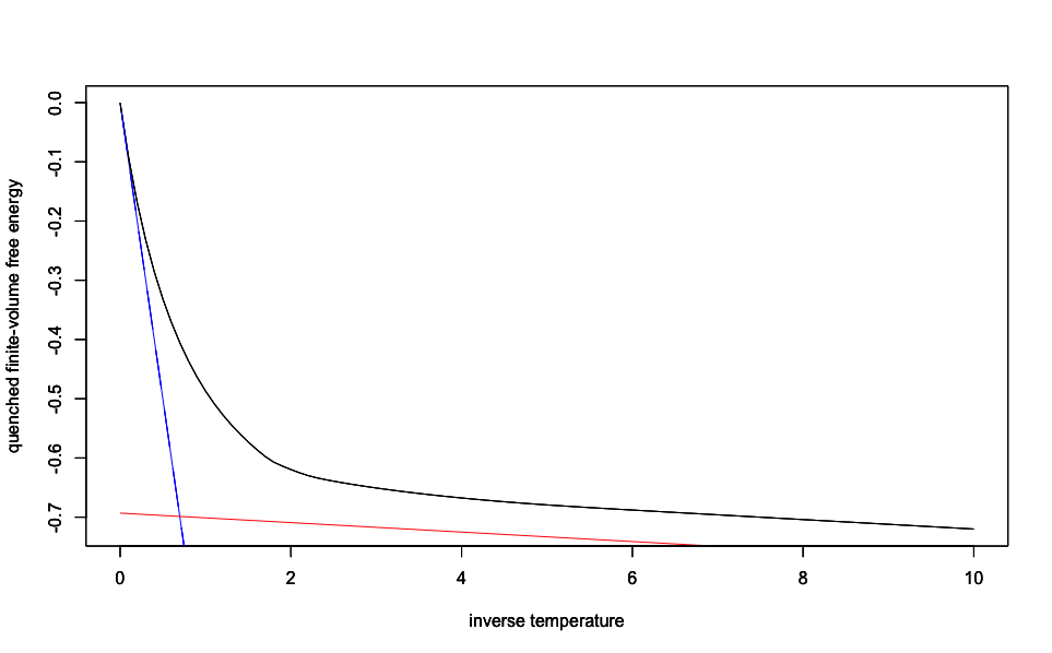
Figure 1. Quenched finite-volume free energy $(1/n)\log\bar{Z}^{\beta,\omega}_{n}$ versus inverse temperature $\beta$ for centered $\pm 1$ i.id. charges $\omega$ and polymer size $n=1000$ as defined in (2.8). The high-temperature lower bound ($-\beta$) and the low-temperature lower bound from (2.61) respectively appear in blue and red.

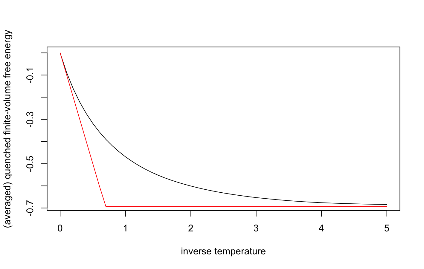
Figure 2. Averaged quenched finite-volume free energy $(1/n){\mathbb{E}}\log\bar{Z}^{\beta,\omega}_{n}$ versus inverse temperature $\beta$ for centered $\pm 1$ i.id. charges $\omega$ and polymer size $n=1000$ as defined in (2.8). We have used $100$ samples to approximate the average over the charge distribution. The lower bound stated in Proposition 2.11 is shown in red.

2.3.2. The LDP for words in a quenched random letter sequence

As we already observed in Section 2.1.3, the present model can be formulated as a statistical mechanics model built on a renewal sequence in the presence of quenched randomness, like the random pinning and copolymer models [13, 17, 18]. In these models, one can visualize the random charge sequence $(\omega_{i})_{i\geq 1}$ as a random letter sequence from which the renewal process $(\tau_{k})_{k\geq 0}$ cuts a word sequence $(Y_{k})_{k\geq 1}$, where $Y_{k}:=(\omega_{i})_{\tau_{k-1}<i\leq\tau_{k}}$ for every $k\geq 1$. Then, the energy or Hamiltonian function may be recast as an appropriate functional applied to the word sequence empirical measure. The purpose of this section is to apply a large deviation principle (LDP) for the empirical measure of such words (when the letter sequence is quenched) in order to obtain a variational formula for the free energy. This LDP at the level of measures was originally introduced by Birkner [3], shortly later generalized to a broader class of renewal tails by Birkner, Greven, den Hollander [4, 5] and successfully applied to the random pinning and copolymer models [6, 7, 10, 14, 20].

To implement this idea, let us first define the grand canonical partition function:

(2.63) $${\mathcal{Z}}_{\beta,\omega}(f):=\sum_{n\geq 1}\bar{Z}_{n,c}^{\beta,\omega}e^{-fn},\qquad f\in{\mathbb{R}}.$$

Note that we use the constrained version of the partition function defined in (2.53). By Theorem 2.10, the free energy is the infimum of those values of $f$ which make the latter sum converge:

(2.64) $$\bar{F}_{\rm que}(\beta)=\inf\{f\in{\mathbb{R}}\colon{\mathcal{Z}}_{\beta,\omega}(f)<\infty\}.$$

By (2.14), we may write

(2.65) $${\mathcal{Z}}_{\beta,\omega}(f) =\sum_{n\geq 1}e^{-fn}\sum_{k\geq 1}\mathrm{E}\Big{[}\exp\Big{(}-\beta\sum_{1\leq i\leq k}\Omega(\tau_{i-1},\tau_{i}]^{2}\Big{)}{\sf 1}_{\{\tau_{k}=n\}}\Big{]}$$

$$=\sum_{k\geq 1}\mathrm{E}\Big{[}\exp\Big{(}-\sum_{i=1}^{k}[\beta\Omega(\tau_{i-1},\tau_{i}]^{2}+f(\tau_{i}-\tau_{i-1})]\Big{)}\Big{]}=:\sum_{k\geq 1}W_{k}^{\beta,\omega}.$$

Using the Large Deviation Principle for words cut out of a quenched random sequence of letters and Varadhan’s lemma [3, Theorem 1 and Corollary 1] we obtain the following ${\mathbb{P}}$-a.s. limit:

(2.66) $$\lim_{k\to\infty}\frac{1}{k}\log W_{k}^{\beta,\omega}=-J(\beta,f),\qquad f>-\log 2,$$

where

(2.67) $$J(\beta,f):=\inf_{Q\in{\mathcal{R}}_{0}}\int[\beta(y_{1,1}+\ldots+y_{1,\ell(y_{1})})^{2}+f\ell(y_{1})]Q(\text{\rm d}y)+H(Q|Q_{0})$$

and with the following notation:

• $Q$ is a probability distribution on sequences of words. Words are elements of $\cup_{\ell\geq 1}{\mathbb{R}}^{\ell}$, and $\ell(y_{1})$ denotes the length of $y_{1}=(y_{1,1},\ldots,y_{1,\ell(y_{1})})$, that is the first word in the sequence $y=(y_{i})_{i\geq 1}$.

• $Q_{0}$ is the probability distribution for i.i.d. words with marginal

  (2.68) $$Q_{0}(\text{\rm d}y_{1})=\sum_{\ell\geq 1}2^{-\ell}\prod_{1\leq i\leq\ell}{\mathbb{P}}(\text{\rm d}y_{1,i}),$$

  that is the one induced by the charge/letter sequence law ${\mathbb{P}}$ (Section 2.1.1) and the geometrically distributed inter-arrival times $(\tau_{k}-\tau_{k-1})_{k\geq 1}$ (Section 2.1.3).

• $H(Q|Q_{0})$ is the specific relative entropy of $Q$ w.r.t. $Q_{0}$, defined as

  (2.69) $$H(Q|Q_{0})=\lim_{n\to\infty}\frac{1}{n}h(Q[(Y_{1},\ldots,Y_{n})\in\cdot]\,|\,Q_{0}[(Y_{1},\ldots,Y_{n})\in\cdot]),$$

  where $h(\cdot|\cdot)$ is the usual relative entropy of one probability measure w.r.t. another and the limit is non-decreasing.

• ${\mathcal{R}}_{0}$ denotes the set of shift-invariant distributions on word sequences which are compatible with ${\mathbb{P}}$, meaning that when one concatenates a typical word sequence into a letter sequence, the empirical distribution of the latter (at the level of processes) converges weakly to ${\mathbb{P}}$, see [3, Equation (8)] for a formal definition.

Note that $J(\beta,f)$ is non-decreasing in both its variables. The fact that (2.66) is not stated for all the possible values of $f$ comes from the lack of boundedness of the function to which we apply Varadhan’s lemma. As in [3] (see the remark around Eq. (19) therein) we use instead an exponential tightness property [12, Condition (4.3.3) in Theorem 4.3.1], hence the restriction $f>-\log 2$. This restriction is harmless since we know from a separate argument that $\bar{F}_{\rm que}(\beta)\geq-\log 2$ for every $\beta>0$, see Proposition 2.11. Combining (2.64), (2.65) and (2.66), we finally obtain the following:

Theorem 2.12.

For every $\beta>0$,

(2.70) $$\bar{F}_{\rm que}(\beta)=\inf\{f\in{\mathbb{R}}\colon J(\beta,f)>0\}.$$

Let us comment on a few elementary bounds obtained from this formula. By plugging $Q=Q_{0}$ into (2.67) we obtain that $J(\beta,f)\leq 2(\beta+f)$, from which we retrieve the elementary Jensen bound $\bar{F}_{\rm que}(\beta)\geq-\beta$. One can also try to restrict the infimum in (2.67) to those $Q$’s under which words are i.i.d. with marginal of the form

(2.71) $$Q(\text{\rm d}y_{1})=\sum_{\ell\geq 1}K(\ell)\prod_{1\leq i\leq\ell}{\mathbb{P}}(\text{\rm d}y_{1,i}),$$

where $K$ ranges over all probability distributions on the set of positive integers. We obtain thereby

(2.72) $$J(\beta,f)\leq\inf_{K}\{(f+\log 2+\beta)m(K)-h(K)\},$$

where $m(K):=\sum_{\ell\geq 1}\ell K(\ell)$ and $h(K):=-\sum_{\ell\geq 1}K(\ell)\log K(\ell)$ are the mean and entropy of $K$, respectively. A simple argument (using Lagrange multipliers) shows that the optimal $K$ follows a geometric distribution, i.e. $K(\ell)=\theta^{\ell-1}(1-\theta)$ for some $\theta\in(0,1)$. Therefore,

(2.73) $$J(\beta,f)\leq\inf_{\theta\in(0,1)}\Big{\{}\frac{f+\log 2+\beta}{1-\theta}+\Big{(}\frac{\theta}{1-\theta}\Big{)}\log\theta+\log(1-\theta)\Big{\}}.$$

The latter is optimal at $\theta_{0}:=\exp(-[f+\log 2+\beta])$, provided $\theta_{0}\in(0,1)$, leading in that case to $J(\beta,f)\leq\log(\exp(f+\log 2+\beta)-1)$, and ultimately to $\bar{F}_{\rm que}(\beta)\geq-\beta$. Unfortunately, this is not any better than the Jensen lower bound. The reason is that this strategy does not take under consideration the charge sequence. In Section 2.4, we shall implement a more refined strategy where each monomer looks at the charge of the following one to decide its state (folded or stretched) and improve thereby our lower bound on the free energy.

2.4. High-temperature estimate on the free energy

This section is primarily focussed on high-temperature estimates on the quenched free energy of the charged polymer, even if some results that we derive en route (namely Theorem 2.13 and Proposition 2.94) are valid at all temperatures.

2.4.1. A lower bound

The starting point of our lower bound is Theorem 2.12. By testing an appropriate probability distribution on word sequences in the variational formula (2.67), we obtain an upper bound on the rate function $J(\beta,f)$, which in turn yields a lower bound on the free energy. The distribution $Q\in{\mathcal{R}}_{0}$ which we test is a tilt of the $\mathrm{Geo}(1/2)$ distribution which looks at pairs of consecutive charges to decide on where to fold the polymer chain, see (2.78) below. In view of Proposition 2.3, it is plausible that a better strategy would look at all pairs of charges, with a decreasing influence for charges that are far-apart, but the implementation of such strategy seems technically much more demanding.

Theorem 2.13.

For every $\beta>0$,

(2.74) $$\bar{F}_{\rm que}(\beta)\geq-\beta+\sup_{0\leq u\leq\log 2}\Big{[}\beta\frac{\sinh(u)}{1+\frac{\sinh(u)}{2}}-\frac{1}{2}u\sinh(u)-\eta(u)\Big{]} ,$$

where

(2.75) $$\eta(u):=\frac{1}{4}[\log(2-e^{u})(2-e^{u})+\log(2-e^{-u})(2-e^{-u})].$$

We readily deduce thereof the following high temperature lower bound:

Corollary 2.14.

As $\beta\to 0$,

(2.76) $$\bar{F}_{\rm que}(\beta)\geq-\beta+\frac{\beta^{2}}{2}[1+o(1)].$$

Remark 2.15.

Expanding the finite-volume free energy at high temperature (see Proposition B.1 for the precise assumptions) and (blindly) interchanging the $\beta\to 0$ and $n\to\infty$ limits leads to the prediction:

(2.77) $$\bar{F}_{\rm que}(\beta)\stackrel{{\scriptstyle(?)}}{{=}}-\beta+\frac{4\beta^{2}}{3}[1+o(1)].$$

However, such naive expansions do not always give the correct values for high-temperatures limits, see e.g. [1] in the context of pinning and copolymer models.

Proof of Theorem 2.13.

For every $u\in[0,\log 2]$, we introduce a law on word sequences $Y=(Y_{i})_{i\geq 1}$, denoted by $Q_{u}$, such that (i) the letter sequence distribution equals the original charge sequence distribution, i.e. $Q_{u}(\omega=\kappa(Y)\in\cdot\,)={\mathbb{P}}(\omega\in\cdot\,)$, where $\kappa$ is the word-to-letter sequence concatenation, and (ii) the length of the first word, denoted by $L$, is distributed as

(2.78) $$Q_{u}(L=\ell\,|\,\omega)=\prod_{1\leq i<\ell}(1-\tfrac{1}{2}e^{u\omega_{i}\omega_{i+1}})\tfrac{1}{2}e^{u\omega_{\ell}\omega_{\ell+1}},\qquad\ell\geq 1.$$

In other words, $L=\inf\{i\geq 1\colon\theta_{i}=1\}$ where $(\theta_{i})_{i\geq 1}$ is a sequence of Bernoulli random variables that are independent (conditionally to $\omega$) and such that

(2.79) $$Q_{u}(\theta_{i}=1\,|\,\omega)=\tfrac{1}{2}e^{u\omega_{i}\omega_{i+1}},\qquad i\geq 1.$$

A similar formula is assumed to hold for the length of the next words, simply by appropriately shifting the letter sequence $\omega$ on the r.h.s. of (2.78). Note that the random variables $(\omega_{i}\omega_{i+1})_{i\geq 1}$ are actually independent and uniformly distributed on $\{-1,1\}$. Following this remark and averaging (2.78) over $\omega$ yields

(2.80) $$Q_{u}(L=\ell)=\Big{(}1-\frac{\cosh(u)}{2}\Big{)}^{\ell-1}\frac{\cosh(u)}{2},\qquad\ell\geq 1,$$

that is the geometric distribution with expectation $2/\cosh(u)$. The reader may check that under $Q_{u}$ the word sequence is a Markov chain with transitions

(2.81) $$\mathfrak{Q}_{u}((\omega_{i})_{1\leq i\leq\ell_{1}},(\omega_{i})_{\ell_{1}<i\leq\ell_{2}}):=2^{\ell_{1}-\ell_{2}}(\tfrac{1}{2}e^{u\omega_{\ell_{1}}\omega_{\ell_{1}+1}})\prod_{\ell_{1}<i<\ell_{2}}(1-\tfrac{1}{2}e^{u\omega_{i}\omega_{i+1}})$$

(the distribution of a given word depends on the last letter of the previous word) and started from the invariant word (probability) distribution

(2.82) $$\pi_{u}(\omega_{1},\ldots,\omega_{\ell}):=2^{-(\ell+1)}\cosh(u)\prod_{1\leq i<\ell}(1-\tfrac{1}{2}e^{u\omega_{i}\omega_{i+1}}).$$

Moreover, words are i.i.d. if and only if $u=0$, in which case one retrieves the law $Q_{0}$ defined in (2.68). From all these observations we deduce that $Q_{u}\in{\mathcal{R}}_{0}$, that is the restriction set of shift-invariant word sequence distributions which are compatible with ${\mathbb{P}}$, see the definition below (2.67).

We may now plug $Q=Q_{u}$ into (2.67), so that we obtain

(2.83) $$J(\beta,f)\leq\beta\int(\omega_{1}+\ldots+\omega_{L})^{2}\text{\rm d}Q_{u}+f\int L\,\text{\rm d}Q_{u}+H(Q_{u}|Q_{0}).$$

We begin with computing the (specific) relative entropy. By (2.69) and the ergodic theorem, we have

(2.84) $$H(Q_{u}|Q_{0}) =\int\log\mathfrak{Q}_{u}(Y_{1},Y_{2})\text{\rm d}Q_{u}-\int\log\pi_{0}(Y_{1})\text{\rm d}Q_{u}$$

$$=\int\Big{[}\sum_{1\leq i<L}\log(2-e^{u\omega_{i}\omega_{i+1}})+u\omega_{L}\omega_{L+1}\Big{]}\text{\rm d}Q_{u}.$$

With the help of Lemma 2.16 below, we find that

(2.85) $$H(Q_{u}|Q_{0})=\frac{2}{\cosh(u)}\Big{(}\eta(u)+\frac{1}{2}u\sinh(u)\Big{)}.$$

Using once again Lemma 2.16, we may compute the contribution of this strategy to the energy term:

(2.86) $$\int(\omega_{1}+\ldots+\omega_{L})^{2}\text{\rm d}Q_{u} =\int L\text{\rm d}Q_{u}+2\sum_{1\leq i<j}\int\omega_{i}\omega_{j}{\sf 1}_{\{L\geq j\}}\text{\rm d}Q_{u}$$

$$=\frac{2}{\cosh(u)}\Big{(}1-\frac{\sinh(u)}{1+\frac{\sinh(u)}{2}}\Big{)}.$$

Summing up the different terms, we finally obtain

(2.87) $$J(\beta,f)\leq\frac{2}{\cosh(u)}\Big{[}\beta\Big{(}1-\frac{\sinh(u)}{1+\frac{\sinh(u)}{2}}\Big{)}+\frac{1}{2}u\sinh(u)+\eta(u)+f\Big{]}.$$

Hence, by Theorem 2.12,

(2.88) $$\bar{F}_{\rm que}(\beta)\geq\beta\Big{(}\frac{\sinh(u)}{1+\frac{\sinh(u)}{2}}-1\Big{)}-\frac{1}{2}u\sinh(u)-\eta(u) ,$$

and the proof is complete. ∎

Proof of Corollary 2.14.

Let us pick $u=C\beta$ in Theorem 2.13, with $C>0$ to be determined later. Noting that, as $u\to 0$,

(2.89) $$\frac{\sinh(u)}{1+\frac{\sinh(u)}{2}}\sim u,\qquad u\sinh(u)\sim u^{2},\qquad\eta(u)=o(u^{2}),$$

we obtain, as $\beta\to 0$,

(2.90) $$\bar{F}_{\rm que}(\beta)\geq-\beta+\beta^{2}(C-C^{2}/2)+o(\beta^{2}),$$

which we optimise by setting $C=1$. ∎

Lemma 2.16.

For every $\Phi\colon\{-1,1\}\mapsto{\mathbb{R}}$ and $u\in[0,\log 2]$,

(2.91) $$\int\Phi(\omega_{i}\omega_{i+1}){\sf 1}_{\{L>i\}}\text{\rm d}Q_{u} =\Big{(}1-\frac{\cosh(u)}{2}\Big{)}^{i-1}\,\frac{\Phi(-1)(2-e^{-u})+\Phi(1)(2-e^{u})}{4},$$

$$\int\Phi(\omega_{i}\omega_{i+1}){\sf 1}_{\{L=i\}}\text{\rm d}Q_{u} =\Big{(}1-\frac{\cosh(u)}{2}\Big{)}^{i-1}\,\frac{\Phi(-1)e^{-u}+\Phi(1)e^{u}}{4},$$

and for every $1\leq i<j$,

(2.92) $$\int\omega_{i}\omega_{j}{\sf 1}_{\{L\geq j\}}\text{\rm d}Q_{u}=\Big{(}1-\frac{\cosh(u)}{2}\Big{)}^{i-1}\Big{(}-\frac{\sinh(u)}{2}\Big{)}^{j-i}.$$

Proof of Lemma 2.16.

Let us start with (2.91). By conditioning on $\omega$ and using (2.78),

(2.93) $$\int\Phi(\omega_{i}\omega_{i+1}){\sf 1}_{\{L>i\}}\text{\rm d}Q_{u} =\int\Phi(\omega_{i}\omega_{i+1})\prod_{1\leq j\leq i}(1-\tfrac{1}{2}e^{u\omega_{j}\omega_{j+1}})\text{\rm d}{\mathbb{P}},$$

$$\int\Phi(\omega_{i}\omega_{i+1}){\sf 1}_{\{L=i\}}\text{\rm d}Q_{u} =\int\Phi(\omega_{i}\omega_{i+1})\prod_{1\leq j<i}(1-\tfrac{1}{2}e^{u\omega_{j}\omega_{j+1}})\tfrac{1}{2}e^{u\omega_{i}\omega_{i+1}}\text{\rm d}{\mathbb{P}}.$$

We conclude by observing that the random variables $(\omega_{i}\omega_{i+1})_{i\geq 1}$ are independent and uniformly distributed in $\{-1,1\}$. The equality in (2.92) is proven in a similar fashion, once we notice that $\omega_{i}\omega_{j}=\prod_{i\leq k<j}\omega_{k}\omega_{k+1}$. ∎

2.4.2. An upper bound

In this section we derive several upper bounds on the quenched free energy through annealing. We start with the following:

Proposition 2.17.

For every $\beta\geq 0$,

(2.94) $$\bar{F}_{\rm que}(\beta)\leq\bar{F}_{\rm ann}(\beta):=-\sup\Big{\{}f\geq 0\colon\sum_{\ell\geq 1}(e^{f}/2)^{\ell}{\mathbb{E}}(e^{-\beta\Omega_{\ell}^{2}})<1\Big{\}}\in[-\log 2,0].$$

Proof of Proposition 2.17.

For ease of notation, let us set

(2.95) $$g_{\beta}(\ell):={\mathbb{E}}(e^{-\beta\Omega_{\ell}^{2}})={\mathbb{E}}(e^{-\beta(\omega_{1}+\ldots+\omega_{\ell})^{2}}),\qquad\ell\geq 1,$$

with the convention $g_{\beta}(0)=1$. Using the i.i.d. assumption on the charges, the annealed partition function equals

(2.96) $${\mathbb{E}}\bar{Z}_{n}^{\beta,\omega}=\mathrm{E}\Big{[}\prod_{x\in{\mathbb{N}}}g_{\beta}(\ell_{n}(x))\Big{]},\qquad\textrm{with }\ell_{n}(x):=\mathrm{card}\{1\leq k\leq n\colon S_{k}=x\}.$$

Using the geometric distribution of the time spent on each visited vertex, we readily obtain

(2.97) $${\mathbb{E}}\bar{Z}_{n}^{\beta,\omega}=2\sum_{k=1}^{n}\sum_{\begin{subarray}{c}\ell_{1},\ldots,\ell_{k}\geq 1\\ \ell_{1}+\ldots+\ell_{k}=n\end{subarray}}\prod_{i=1}^{k}g_{\beta}(\ell_{i})2^{-\ell_{i}},$$

from which we deduce the annealed grand canonical partition function

(2.98) $$\sum_{n\geq 1}{\mathbb{E}}\bar{Z}_{n}^{\beta,\omega}e^{fn}=2\sum_{k\geq 1}\Big{[}\sum_{\ell\geq 1}(e^{f}/2)^{\ell}g_{\beta}(\ell)\Big{]}^{k}.$$

The extra factor $2$ in front of the sums in (2.97) and (2.98) comes from the fact that $S_{1}=1$. Thus, the annealed free energy, which could alternatively be defined as

(2.99) $$\bar{F}_{\rm ann}(\beta)=\limsup_{n\to\infty}\frac{1}{n}\log{\mathbb{E}}\bar{Z}_{n}^{\beta,\omega},$$

has the variational representation displayed in (2.94). The first inequality therein follows from Theorem 2.10 and the standard Jensen bound:

(2.100) $${\mathbb{E}}\log\bar{Z}_{n}^{\beta,\omega}\leq\log{\mathbb{E}}\bar{Z}_{n}^{\beta,\omega}.$$

The fact that the annealed free energy is non-positive clearly follows from (2.99). The fact that it is bounded from below by $(-\log 2)$ follows by checking that

(2.101) $$\sum_{\ell\geq 1}(e^{\log 2}/2)^{\ell}g_{\beta}(\ell)=\sum_{\ell\geq 1}g_{\beta}(\ell)\geq\sum_{\ell\in 2{\mathbb{N}}}{\mathbb{P}}(\Omega_{\ell}=0)=+\infty,$$

since ${\mathbb{P}}(\Omega_{\ell}=0)\sim\mathrm{(cst.)}\,\ell^{-1/2}$ as $\ell\to\infty$ along even integers. ∎

We first use Proposition 2.17 to derive a high-temperature upper bound.

Proposition 2.18 (Binary charges).

As $\beta\to 0$,

(2.102) $$\bar{F}_{\rm que}(\beta)\leq\bar{F}_{\rm ann}(\beta)\leq-\beta+2\beta^{2}+o(\beta^{2}).$$

Proposition 2.19 (standard Gaussian charges).

As $\beta\to 0$,

(2.103) $$\bar{F}_{\rm que}(\beta)\leq\bar{F}_{\rm ann}(\beta)\leq-\beta+3\beta^{2}+o(\beta^{2}).$$

Proof of Proposition 2.18.

Recall the expression of the annealed free energy in (2.94). Replacing the $(e^{f}/2)$ therein by $z<1$, using the inequality $e^{-y}\leq 1-y+\tfrac{1}{2}y^{2}$ for every $y\geq 0$, and using Lemma A.1, we have

(2.104) $$\sum_{\ell\geq 1}z^{\ell}{\mathbb{E}}(e^{-\beta\Omega_{\ell}^{2}})\leq\sum_{\ell\geq 1}z^{\ell}[1-(\beta+\beta^{2})\ell+\tfrac{3}{2}\beta^{2}\ell^{2}].$$

Using Lemma A.2 with ${\sf c}_{1}(\beta)=-\beta-\beta^{2}$ and ${\sf c}_{2}(\beta)=\tfrac{3}{2}\beta^{2}$, we obtain

(2.105) $$2z^{3}+({\sf u}_{1}(\beta)-5)z^{2}+({\sf u}_{2}(\beta)+4)z-1<0\Rightarrow\sum_{\ell\geq 1}z^{\ell}{\mathbb{E}}(e^{-\beta\Omega_{\ell}^{2}})<1,$$

where

(2.106) $${\sf u}_{1}(\beta)=\beta+\tfrac{5}{2}\beta^{2},\qquad{\sf u}_{2}(\beta)=-\beta+\tfrac{1}{2}\beta^{2}.$$

Using Lemma A.3, we see that the condition on the l.h.s. of (3.7) is satisfied if

(2.107) $$z<z(\beta):=z_{0}({\sf u}_{1}(\beta),{\sf u}_{2}(\beta))=\tfrac{1}{2}+\tfrac{1}{2}\beta-\tfrac{3}{4}\beta^{2}+o(\beta^{2}).$$

Therefore,

(2.108) $$\bar{F}_{\rm ann}(\beta)\leq-\log(2z(\beta))=-\beta+2\beta^{2}+o(\beta^{2}).$$

∎

Proof of Proposition 2.19.

Same as Proposition 2.18 with ${\mathbb{E}}(\Omega_{\ell}^{4})=3\ell^{2}$, hence ${\sf c}_{1}(\beta)=-\beta$ and ${\sf c}_{2}(\beta)=\tfrac{3}{2}\beta^{2}$. ∎

2.5. Low-temperature estimate on the free energy

We may also use Proposition 2.17 to derive low-temperature upper bounds.

Proposition 2.20 (Gaussian case).

As $\beta\to\infty$,

(2.109) $$\bar{F}_{\rm que}(\beta)\leq\bar{F}_{\rm ann}(\beta)=-\log 2+\frac{\pi}{2\beta}(1+o(1)),$$

Proof of Proposition 2.20.

The inequality has already been proved so we focus on the low-temperature expansion. Recall the expression of the annealed free energy in (2.94). In the case of standard Gaussian charges, we can explicitely compute

(2.110) $${\mathbb{E}}(e^{-\beta\Omega_{\ell}^{2}})=\frac{1}{\sqrt{1+2\beta\ell}}.$$

Considering $f(\beta):=\log 2-C/\beta$, with $C>0$, we obtain

(2.111) $$\sum_{\ell\geq 1}(e^{f(\beta)}/2)^{\ell}{\mathbb{E}}(e^{-\beta\Omega_{\ell}^{2}})=\sum_{\ell\geq 1}\frac{e^{-C\ell/\beta}}{\sqrt{1+2\beta\ell}}.$$

Dropping one in the square root above yields the following upper bound:

(2.112) $$\sum_{\ell\geq 1}(e^{f(\beta)}/2)^{\ell}{\mathbb{E}}(e^{-\beta\Omega_{\ell}^{2}})\leq\sum_{\ell\geq 1}\frac{e^{-C\ell/\beta}}{\sqrt{2\beta\ell}}=\frac{1}{\beta}\sum_{\ell\geq 1}\frac{e^{-C\ell/\beta}}{\sqrt{2\ell/\beta}},$$

which converges in the large $\beta$ limit, by a Riemann approximation, to

(2.113) $$\int_{0}^{\infty}(2x)^{-1/2}e^{-Cx}\text{\rm d}x=\frac{1}{\sqrt{C}}\int_{0}^{\infty}(2x)^{-1/2}e^{-x}\text{\rm d}x\stackrel{{\scriptstyle(y^{2}=2x)}}{{=}}\sqrt{\frac{\pi}{2C}}.$$

The upper bound that we have just used can be complemented by the following lower bound:

(2.114) $$\frac{e^{-C\ell/\beta}}{\sqrt{1+2\beta\ell}}=\frac{e^{-C\ell/\beta}}{\sqrt{2\beta\ell}}\times\frac{1}{\sqrt{1+(2\beta\ell)^{-1}}}\geq\frac{e^{-C\ell/\beta}}{\sqrt{2\beta\ell}}\times\frac{1}{\sqrt{1+(2\beta)^{-1}}},\qquad\ell\geq 1,$$

which allows to complete the proof. ∎

Remark 2.21 (Binary case).

The annealed upper bound obtained in the case of binary charges is quite rough. Indeed, one can show that

(2.115) $$\lim_{\beta\to\infty}\bar{F}_{\rm ann}(\beta)=-\frac{\log 3}{2}>-\log 2.$$

Existence follows from monotonicity. In order to obtain the value of the limit, we first observe that

(2.116) $$0\leq\sum_{\ell\geq 1}z^{\ell}{\mathbb{E}}(e^{-\beta\Omega_{\ell}^{2}})-\sum_{\ell\geq 1}z^{2\ell}{\mathbb{P}}(\Omega_{2\ell}=0)\leq\frac{e^{-\beta}z}{1-z},\qquad 0\leq z<1.$$

Indeed, by splitting the leftmost sum according to the parity of $\ell$, we obtain:

(2.117) $$0\leq \sum_{\begin{subarray}{c}\ell\geq 1\\ \ell\in 2{\mathbb{Z}}\end{subarray}}z^{\ell}{\mathbb{E}}(e^{-\beta\Omega_{\ell}^{2}})-\sum_{\begin{subarray}{c}\ell\geq 1\\ \ell\in 2{\mathbb{Z}}\end{subarray}}z^{\ell}{\mathbb{P}}(\Omega_{\ell}=0)\leq e^{-\beta}\sum_{\begin{subarray}{c}\ell\geq 1\\ \ell\in 2{\mathbb{Z}}\end{subarray}}z^{\ell},$$

$$0\leq \sum_{\begin{subarray}{c}\ell\geq 1\\ \ell\in 2{\mathbb{Z}}+1\end{subarray}}z^{\ell}{\mathbb{E}}(e^{-\beta\Omega_{\ell}^{2}})\leq e^{-\beta}\sum_{\begin{subarray}{c}\ell\geq 1\\ \ell\in 2{\mathbb{Z}}+1\end{subarray}}z^{\ell},$$

from which (2.116) readily follows. The rightmost sum in (2.116) can be computed explicitly, see e.g. [21, Chapter I, E2]

(2.118) $$\sum_{\ell\geq 1}z^{2\ell}{\mathbb{P}}(\Omega_{2\ell}=0)=\frac{1}{\sqrt{1-z^{2}}}-1,\qquad|z|<1.$$

Combining the above expression with (2.116) and (2.94) gives (2.115). The main contribution to the annealed partition function, in the large $\beta$ limit, is thus given by charge distributions such that $\Omega_{n}(x)=0$ for every $x\in\{S_{1},\ldots,S_{n}\}$. This indicates that any attempt to improve the annealed bound by means of constrained annealing with a linear potential, that is

(2.119) $${\mathbb{E}}\log\bar{Z}_{n}^{\beta,\omega}\leq\log{\mathbb{E}}[\bar{Z}_{n}^{\beta,\omega}\exp(\lambda\Omega_{n})],\qquad\lambda\in{\mathbb{R}},$$

(also known as first order Morita approximation) is bound to fail. See e.g.  [9] for a reference on constrained annealing in the context of pinning

3. Corrections to the undirected model

In this section we correct two propositions from [8, Appendix D] concerning the undirected quenched charged polymer. The statement of the first proposition therein (Proposition D.1) is left unchanged, although we stress that the result holds in any dimension. The proof however must be corrected. In the second proposition (Proposition D.2), the sufficient condition for ballistic behaviour in dimension one is amended.

Although this section is independent of the rest of the paper, we prefer to stick to our notation (that is anyway not far from the one used in [8]) in order to make the paper more self-contained. The two major differences with the directed model from Section 2 are the following:

• $\mathrm{P}$ denotes the law of simple random walk $S=(S_{i})_{i\in{\mathbb{N}}_{0}}$ (started at the origin) on ${\mathbb{Z}}^{d}$, i.e. $(S_{i}-S_{i-1})_{i\in{\mathbb{N}}}$ is a sequence of i.i.d. random variables uniformly distributed on the $2d$ unit vectors.

• ${\mathbb{P}}$ denotes the law of i.i.d. real-valued random variables $\omega=(\omega_{i})_{i\in{\mathbb{N}}}$ with zero mean, unit variance and finite exponential moments, i.e. $M(\delta):={\mathbb{E}}(e^{\delta\omega_{1}})<\infty$ for every $\delta\geq 0$. Here, we also allow biased charge distributions: for every $\delta\geq 0$, we let ${\mathbb{P}}_{\delta}$ be the tilted probability measure uniquely defined by the property:

  (3.1) $${\mathbb{P}}_{\delta}(A)={\mathbb{E}}(e^{\delta\Omega_{n}-n\log M(\delta)}{\sf 1}_{A}),\qquad\forall n\in{\mathbb{N}},\quad\forall A\in\sigma(\omega_{1},\ldots,\omega_{n}).$$

  Note that the random variables $(\omega_{i})_{i\in{\mathbb{N}}}$ remain i.i.d. under ${\mathbb{P}}_{\delta}$ and that ${\mathbb{P}}_{0}={\mathbb{P}}$.

In addition, we let

(3.2) $$R_{n}(S):=\mathrm{card}\{S_{1},\ldots,S_{n}\}$$

be the number of distinct vertices visited by the random walk between time $1$ and time $n$.

The proposition below corresponds to [8, Proposition D.1]. The lower bound in the proof must be corrected. Also, we stress that the result is valid in any dimension.

Proposition 3.1.

Let $d\geq 1$. Suppose that $\delta,\beta\in(0,\infty)$. Then there exist $c_{1},c_{2}>0$ (depending on $\delta,\beta$) such that, for ${\mathbb{P}}_{\delta}$-a.e. $\omega$,

(3.3) $$\bar{}\mathrm{P}_{n}^{\beta,\omega}(R_{n}(S)\leq c_{1}n)\leq e^{-c_{2}n+o(n)}.$$

Proof of Proposition 3.1.

Let $\pi$ be the one-sided path that takes right-steps only, i.e., $\pi_{i}=(i,0,\ldots 0)$ for $i\in\mathbb{N}_{0}$. Let us denote by $\bar{H}_{n}^{\omega}(S)$ the Hamiltonian in (2.7) and estimate

(3.4) $$\bar{Z}_{n}^{\beta,\omega}\geq\,\mathrm{E}\Big{[}e^{-\beta\bar{H}_{n}^{\omega}(S)}\,{\sf 1}_{\{S_{i}=\pi_{i}\,\forall\,1\leq i\leq n\}}\Big{]}=(\tfrac{1}{2d})^{n}\,e^{-\beta\sum_{i=1}^{n}\omega_{i}^{2}}=(\tfrac{1}{2d})^{n}\,e^{-\beta{\mathbb{E}}_{\delta}(\omega_{1}^{2})n+o(n)},$$

where the $o(\cdot)$ holds ${\mathbb{P}}_{\delta}$-a.s, by the law of large numbers. Moreover, by Jensen’s inequality we have (recall (2.8), (2.9) and the definition of $\ell_{n}$ in (2.43))

(3.5) $$\bar{H}_{n}^{\omega}(S) =\sum_{{x\in\mathbb{Z}\colon}\atop{\ell_{n}(x)>0}}\left(\sum_{i=1}^{n}\omega_{i}{\sf 1}_{\{S_{i}=x\}}\right)^{2}=R_{n}(S)\left[\frac{1}{R_{n}(S)}\sum_{{x\in\mathbb{Z}\colon}\atop{\ell_{n}(x)>0}}\left(\sum_{i=1}^{n}\omega_{i}{\sf 1}_{\{S_{i}=x\}}\right)^{2}\right]$$

$$\geq R_{n}(S)\left(\frac{1}{R_{n}(S)}\sum_{{x\in\mathbb{Z}\colon}\atop{\ell_{n}(x)>0}}\sum_{i=1}^{n}\omega_{i}{\sf 1}_{\{S_{i}=x\}}\right)^{2}=\frac{1}{R_{n}(S)}\,\Omega_{n}^{2}.$$

Combining (3.4–LABEL:eq:3), we obtain

(3.6) $$\bar{}\mathrm{P}_{n}^{\beta,\omega}(R_{n}(S)\leq c_{1}n) \leq e^{\beta[{\mathbb{E}}_{\delta}(\omega_{1}^{2})+o(1)]n}\,(2d)^{n}\,\mathrm{E}\left[\exp\left\{-\frac{\beta}{R_{n}(S)}\,\Omega_{n}^{2}\right\}\,{\sf 1}_{\{R_{n}(S)\leq c_{1}n\}}\right]$$

$$\leq\exp\left\{-\beta n\left[\frac{1}{c_{1}n^{2}}\,\Omega_{n}^{2}-{\mathbb{E}}_{\delta}(\omega_{1}^{2})-\tfrac{\log(2d)}{\beta}+o(1)\right]\right\}.$$

Note that ${\mathbb{E}}_{\delta}(\omega_{1}^{2})=m(\delta)^{2}+m^{\prime}(\delta)$, where $m(\delta):=(\log M)^{\prime}(\delta)$. By the strong law of large numbers for $\omega$, we have $\lim_{n\to\infty}n^{-1}\Omega_{n}=m(\delta)>0$ for ${\mathbb{P}}_{\delta}$-a.e. $\omega$, and so the term between square brackets equals $c_{3}[1+o(1)]$ with $c_{3}=(\tfrac{1}{c_{1}}-1)m(\delta)^{2}-m^{\prime}(\delta)-\tfrac{\log(2d)}{\beta}$. Therefore, by choosing $c_{1}>0$ small enough so that $c_{3}>0$, we get (3.3) with $c_{2}=\beta c_{3}$. ∎

The following proposition corrects [8, Proposition D.2]. The correction comes from the changes in the proof of Proposition 3.1.

Proposition 3.2.

Assume that $d=1$ and that $\beta,\delta\in(0,\infty)$ satisfy

(3.7) $$m(\delta)^{2}-m^{\prime}(\delta)>\frac{\log 2}{\beta}.$$

Then, there exists $\varepsilon=\varepsilon(\delta,\beta)>0$ such that:

(3.8) $$\lim_{n\to\infty}\bar{}\mathrm{P}_{n}^{\beta,\omega}\big{(}n^{-1}S_{n}>\varepsilon\mid S_{n}>0\big{)}=1.$$

Remark 3.3.

When ${\mathbb{P}}(\omega_{1}\in\cdot)={\mathcal{N}}(0,1)$ then $m(\delta)=\delta$ and $m^{\prime}(\delta)=1$, so that the condition in (3.7) is equivalent to $\delta^{2}>1+(\log 2)/\beta$ (that is a non-empty condition). When ${\mathbb{P}}(\omega_{1}\in\cdot)$ is the uniform probability measure on $\{-1,1\}$ then $m(\delta)=\tanh(\delta)$ and $m^{\prime}(\delta)=1-\tanh(\delta)^{2}$, so that the condition in (3.7) is equivalent to $2\tanh(\delta)^{2}>1+(\log 2)/\beta$. The latter condition is non-empty if and only if $\beta>\log 2$. A similar remark can be made for all bounded charge distributions.

Proof of Proposition 3.2.

Recall the value of $c_{3}$ in the proof of Proposition 3.1. If (3.7) is satisfied then we can choose $c_{1}>\tfrac{1}{2}$ in Proposition 3.1 and use the inequality

(3.9) $$\frac{\left|\{x\in{\mathbb{Z}}\colon\,\ell_{n}(x)=1\}\right|}{n}\geq\frac{2R_{n}(S)}{n}-1$$

to conclude that a positive fraction of the sites are visited precisely once. Consequently, if the polymer chain chooses to go to the right, then $S_{n}/n$ has a strictly positive $\liminf$. ∎

4. Conclusion and perspectives

For the directed charged polymer with quenched centered charges, we have reviewed and provided detailed proofs of past results concerning the freezing transition predicted by Derrida, Griffiths and Higgs. We showed that the quenched free energy enjoys a variational representation based on a quenched (or conditional) large deviation principle, much like pinning and copolymer models. Lower bounds are derived from this variational formula, while upper bounds are obtained through annealing. It is however not clear to us whether the freezing transition can be read from the free energy. Nevertheless, we hope that the efforts to obtain sharper estimates will lead to a better understanding of the model.

For the undirected charged polymer with quenched biased charges, one can show that the number of visited vertices is proportional to a positive fraction of the chain, with large probability. This property may be upgraded to true ballistic behavior, at least for a large enough charge bias, with an extra condition on the temperature for some charge distributions.

Let us finally close the paper with a (non-exhaustive) list of unsettled issues.

• For the directed model:

  1. Settle Items (1) and (2) in Conjecture 2.1.

  2. Give a rigorous proof for the existence of a low temperature regime in the case of random centered charges, as in Item (3) in Conjecture 2.1.

  3. What is the critical temperature for the di-block polymer from (2.18)? The best estimate so far is $\log(\frac{1+\sqrt{5}}{2})\leq\beta_{c}^{\rm di-block}\leq 2\log 2$.

  4. Is the inequality $\bar{F}_{\rm que}(\beta)\geq-\log 2$ strict? Is it valid beyond the binary charge distribution? The strategy used in the proof of Item (2) in Proposition 2.11 could be adapted to other charge distributions (e.g. Gaussian charges) by folding the chain along the sequence of stopping times defined by $\sigma_{0}=0$ and

     (4.1) $$\sigma_{i}=\min\{k>\sigma_{i-1}\colon\Omega_{k}>\Omega_{\sigma_{i-1}}\},\qquad i\in{\mathbb{N}},$$

     instead of (2.59) (assuming w.l.o.g. that $\Omega_{n}>0$). However, the fact that we must stop at $i_{n}:=\min\{i\in{\mathbb{N}}\colon\Omega_{\sigma_{i}}\geq\Omega_{n}\}$, that is not a stopping time, would probably lead to cumbersome technicalities.

  5. Is there a minimizer for the variational problem in (2.67)? If so, is it unique?

  6. Is the quenched free energy analytic as a function of the inverse temperature?

  7. Find the value of the constant $\mathsf{C}$ in the high temperature expansion

     (4.2) $$\bar{F}_{\rm que}(\beta)=-\beta+\mathsf{C}\beta^{2}+o(\beta^{2}),\qquad\beta\to 0.$$

     Is it universal? Our best estimate so far is $1/2\leq\mathsf{C}\leq 2$ for binary charges and $1/2\leq\mathsf{C}\leq 3$ for Gaussian charges.

  8. Can the lower bound in Theorem 2.13 be improved by considering a more subtle strategy (looking beyond consecutive monomers)?

  9. Can we prove that $\bar{F}_{\rm que}(\beta)\sim-\log 2$ as $\beta\to\infty$ in the case of binary charges? An upper bound is missing.

• For the undirected model:

  1. Can we prove ballistic behavior for every $\delta,\beta\in(0,\infty)$?

  2. What can be said about the case of neutral charges ($\beta=0$)?

Appendix A Technical estimates

Lemma A.1.

In the case of $\{-1,1\}$-valued centered i.i.d. charges, for every $\ell\geq 1$,

(A.1) $${\mathbb{E}}(\Omega_{\ell}^{4})=3\ell^{2}-2\ell.$$

Proof of Lemma A.1.

We have

(A.2) $${\mathbb{E}}(\Omega_{\ell}^{4})={\mathbb{E}}\Big{(}\Big{[}\ell+2\sum_{1\leq i<j\leq\ell}\omega_{i}\omega_{j}\Big{]}^{2}\Big{)}=\ell^{2}+4{\mathbb{E}}\Big{(}\sum_{\begin{subarray}{c}1\leq i<j\leq\ell\\ 1\leq u<v\leq\ell\end{subarray}}\omega_{i}\omega_{j}\omega_{u}\omega_{v}\Big{)},$$

and the result follows by noticing that only the terms for which $i=u$ and $j=v$ give a nonzero (and actually unit) contribution to the last expectation. ∎

Lemma A.2.

Let $|z|<1$. Then,

(A.3) $$\sum_{\ell\geq 1}z^{\ell}(1+{\sf c}_{1}\ell+{\sf c}_{2}\ell^{2})<1\Leftrightarrow 2z^{3}+({\sf u}_{1}-5)z^{2}+({\sf u}_{2}+4)z-1<0,$$

where

(A.4) $${\sf u}_{1}={\sf c}_{2}-{\sf c}_{1},\qquad{\sf u}_{2}={\sf c}_{1}+{\sf c}_{2}.$$

Proof of Lemma A.2.

The sum in the l.h.s. of (A.3) equals

(A.5) $$\sum_{\ell\geq 1}z^{\ell}+[{\sf c}_{1}+{\sf c}_{2}]\sum_{\ell\geq 1}\ell z^{\ell}+{\sf c}_{2}\sum_{\ell\geq 1}\ell(\ell-1)z^{\ell}=\frac{z}{1-z}+\frac{[{\sf c}_{1}+{\sf c}_{2}]z}{(1-z)^{2}}+\frac{2{\sf c}_{2}z^{2}}{(1-z)^{3}}.$$

The lemma follows from a straightforward computation. ∎

Lemma A.3.

For every ${\sf u}\in{\mathbb{R}}^{2}$ and $z\in{\mathbb{R}}$, let

(A.6) $$P_{\sf u}(z)=2z^{3}+({\sf u}_{1}-5)z^{2}+({\sf u}_{2}+4)z-1.$$

There exists a neighborhood of the origin ${\mathcal{N}}\subseteq{\mathbb{R}}^{2}$ and a function ${\sf u}\in{\mathcal{N}}\mapsto z_{0}({\sf u})$ such that, for every $u\in{\mathcal{N}}$ such that ${\sf u}_{1}+{\sf u}_{2}>0$, $z_{0}({\sf u})$ is the only root of $P_{\sf u}$ in $(-\infty,1)$. Moreover,

(A.7) $$z_{0}({\sf u})=\frac{1}{2}-\frac{{\sf u}_{1}}{2}-{\sf u}_{2}+2{\sf u}_{1}^{2}+6{\sf u}_{2}^{2}+7{\sf u}_{1}{\sf u}_{2}+o(\|{\sf u}\|^{2}),\qquad{\sf u}\to 0.$$

Proof of Lemma A.3.

First, observe that

(A.8) $$P_{0}(z)=(2z-1)(z-1)^{2}$$

admits $1/2$ as a simple root. The result follows from the Implicit Function Theorem and an explicit second-order Taylor expansion. Letting

(A.9) $$z_{0}({\sf u})=\frac{1}{2}+\langle({\sf D}z_{0})(0),{\sf u}\rangle+\frac{1}{2}\langle{\sf u},({\sf D}^{2}z_{0})(0){\sf u}\rangle+o(\|{\sf u}\|^{2}),\qquad{\sf u}\to 0,$$

(with column vectors) we obtain

(A.10) $$0 =P_{\sf u}(z_{0}({\sf u}))=P_{0}(z_{0}({\sf u}))+{\sf u}_{1}z_{0}({\sf u})^{2}+{\sf u}_{2}z_{0}({\sf u})$$

$$=P_{0}^{\prime}(\tfrac{1}{2})[z_{0}({\sf u})-\tfrac{1}{2}]+\tfrac{1}{2}P_{0}^{\prime\prime}(\tfrac{1}{2})[z_{0}({\sf u})-\tfrac{1}{2}]^{2}$$

$$\qquad+\tfrac{1}{4}{\sf u}_{1}+{\sf u}_{1}[z_{0}({\sf u})-\tfrac{1}{2}]+\tfrac{1}{2}{\sf u}_{2}+{\sf u}_{2}[z_{0}({\sf u})-\tfrac{1}{2}]+o(\|{\sf u}\|^{2})$$

$$=\langle\tfrac{1}{2}({\sf D}z_{0})(0)+(\tfrac{1}{4},\tfrac{1}{2})^{\intercal},{\sf u}\rangle$$

$$\qquad+\langle{\sf u},[\tfrac{1}{4}({\sf D}^{2}z_{0})(0)-2({\sf D}z_{0})(0)({\sf D}z_{0})(0)^{\intercal}+(1,1)^{\intercal}({\sf D}z_{0})(0)^{\intercal}]{\sf u}\rangle+o(\|{\sf u}\|^{2}).$$

Therefore,

(A.11) $$({\sf D}z_{0})(0)=\left(\begin{array}[]{c}-1/2\\ -1\end{array}\right),\qquad({\sf D}^{2}z_{0})(0)=\left(\begin{array}[]{cc}4&7\\ 7&12\end{array}\right).$$

The restriction that ${\sf u}_{1}+{\sf u}_{2}>0$ in the statement comes from the fact that $P_{\sf u}(1)={\sf u}_{1}+{\sf u}_{2}$ and allows us to verify that $z_{0}(\mathsf{u})$ is indeed the only root in $(-\infty,1)$ rather than in a neighborhood of $1/2$. ∎

Appendix B High-temperature expansion of the finite-volume free energy

In this section we provide the necessary details for the computation behind Remark 2.15.

Proposition B.1.

In addition to the $\omega_{i}$’s being i.i.d. square integrable random variables with zero mean and unit variance, we assume that ${\mathbb{E}}(\omega_{1}^{4})<\infty$. For every $n\in{\mathbb{N}}$, the finite-volume (averaged) quenched free energy has the following high-temperature ($\beta\to 0$) expansion:

(B.1) $$\frac{1}{n}{\mathbb{E}}\log\bar{Z}_{n}^{\beta,\omega}=-\beta+\mathfrak{c}_{n}\beta^{2}+o(\beta^{2}),\qquad\text{with}\quad\lim_{n\to\infty}\mathfrak{c}_{n}=4/3.$$

Proof of Proposition B.1.

Let $n\in{\mathbb{N}}$. Expanding the exponential in (2.8), we have

(B.2) $$\bar{Z}_{n}^{\beta,\omega}=1-\beta\sum_{x\in{\mathbb{N}}}\mathrm{E}[\Omega_{n}(x)^{2}]+[1+o(1)]\frac{\beta^{2}}{2}\sum_{x,y\in{\mathbb{N}}}\mathrm{E}[\Omega_{n}(x)^{2}\Omega_{n}(y)^{2}].$$

We now apply the logarithm and expand it up to the second-order term. Using that

(B.3) $$\sum_{x\in{\mathbb{N}}}{\mathbb{E}}\mathrm{E}[\Omega_{n}(x)^{2}]=\sum_{x\in{\mathbb{N}}}\ell_{n}(x)=n,$$

we find thereby:

(B.4) $${\mathbb{E}}\log\bar{Z}_{n}^{\beta,\omega}=-\beta n+[1+o(1)]\frac{\beta^{2}}{2}\mathsf{C}_{n},$$

where

(B.5) $$\mathsf{C}_{n} :=\sum_{x,y\in{\mathbb{N}}}{\mathbb{E}}\operatorname{\mathrm{C}ov}(\Omega_{n}(x)^{2},\Omega_{n}(y)^{2})$$

$$=\sum_{x,y\in{\mathbb{N}}}{\mathbb{E}}\mathrm{E}^{\otimes 2}[\Omega_{n}(x)^{2}\Omega_{n}(y)^{2}-\Omega_{n}(x)^{2}\widetilde{\Omega}_{n}(y)^{2}],$$

and $\widetilde{S}$ is a replica (i.e. independent copy) of $S$ (but the fields $\Omega_{n}$ and $\widetilde{\Omega}_{n}$ are built on a common sequence of charges $\omega$). Recalling (2.9) and expanding all the squares in the above expression, $\mathsf{C}_{n}$ is found to be equal to:

(B.6) $$\sum_{\begin{subarray}{c}x,y\in{\mathbb{N}}\\ 1\leq i,j,k,\ell\leq n\end{subarray}}{\mathbb{E}}(\omega_{i}\omega_{j}\omega_{k}\omega_{\ell})[\mathrm{P}(S_{i}=S_{j}=x,S_{k}=S_{\ell}=y)-\mathrm{P}(S_{i}=S_{j}=x)\mathrm{P}(S_{k}=S_{\ell}=y)].$$

Due to our set of assumptions on the charge sequence $\omega$, only the four following cases may contribute to the sum:

1. $i=j=k=\ell$;

2. $i=j$ and $k=\ell$, but $i\neq k$;

3. $i=k$ and $j=\ell$, but $i\neq j$;

4. $i=\ell$ and $j=k$, but $i\neq j$.

The reader may check that Cases (1) and (2) give a zero contribution (once we sum over $x$ and $y$) while Cases (3) and (4) give the same contribution. Therefore, as $n\to\infty$,

(B.7) $$\mathsf{C}_{n}=4\sum_{1\leq i<j\leq n}[\mathrm{P}(S_{i}=S_{j})-\mathrm{P}(S_{i}=S_{j})^{2}]\\ \sim 4n\sum_{\ell\geq 1}[2^{-\ell}-4^{-\ell}]=\frac{8n}{3},$$

which completes the proof. ∎

References

- [1] Q. Berger, F. Caravenna, J. Poisat, R. Sun, and N. Zygouras. The critical curves of the random pinning and copolymer models at weak coupling. Comm. Math. Phys., 326(2):507–530, 2014.
- [2] Q. Berger, F. den Hollander, and J. Poisat. Annealed scaling for a charged polymer in dimensions two and higher. J. Phys. A, 51(5):054002, 37, 2018.
- [3] M. Birkner. Conditional large deviations for a sequence of words. Stochastic Process. Appl., 118(5):703–729, 2008.
- [4] M. Birkner, A. Greven, and F. den Hollander. Quenched large deviation principle for words in a letter sequence. Probab. Theory Related Fields, 148(3-4):403–456, 2010.
- [5] M. Birkner, A. Greven, and F. d. Hollander. Correction to: Quenched large deviation principle for words in a letter sequence. Probab. Theory Related Fields, 187(1-2):523–569, 2023.
- [6] E. Bolthausen, F. den Hollander, and A. A. Opoku. A copolymer near a selective interface: variational characterization of the free energy. Ann. Probab., 43(2):875–933, 2015.
- [7] F. Caravenna and F. den Hollander. Phase transitions for spatially extended pinning. Probab. Theory Related Fields, 181(1-3):329–375, 2021.
- [8] F. Caravenna, F. den Hollander, N. Pétrélis, and J. Poisat. Annealed scaling for a charged polymer. Math. Phys. Anal. Geom., 19(1):Art. 2, 87, 2016.
- [9] F. Caravenna and G. Giacomin. On constrained annealed bounds for pinning and wetting models. Electron. Comm. Probab., 10:179–189, 2005.
- [10] D. Cheliotis and F. den Hollander. Variational characterization of the critical curve for pinning of random polymers. Ann. Probab., 41(3B):1767–1805, 2013.
- [11] F. Comets. Directed polymers in random environments, volume 2175 of Lecture Notes in Mathematics. Springer, Cham, 2017. Lecture notes from the 46th Probability Summer School held in Saint-Flour, 2016.
- [12] A. Dembo and O. Zeitouni. Large deviations techniques and applications, volume 38 of Stochastic Modelling and Applied Probability. Springer-Verlag, Berlin, 2010. Corrected reprint of the second (1998) edition.
- [13] F. den Hollander. Random polymers, volume 1974 of Lecture Notes in Mathematics. Springer-Verlag, Berlin, 2009. Lectures from the 37th Probability Summer School held in Saint-Flour, 2007.
- [14] F. den Hollander and A. A. Opoku. Copolymer with pinning: variational characterization of the phase diagram. J. Stat. Phys., 152(5):846–893, 2013.
- [15] B. Derrida, R. Griffiths, and P. Higgs. A model of directed random walks with random selfinteractions. Europhys. Lett., 18:361–366, 1992.
- [16] B. Derrida and P. G. Higgs. Low-temperature properties of directed walks with random self-interactions. J. Phys. A, 27(16):5485–5493, 1994.
- [17] G. Giacomin. Random polymer models. Imperial College Press, London, 2007.
- [18] G. Giacomin. Disorder and critical phenomena through basic probability models, volume 2025 of Lecture Notes in Mathematics. Springer, Heidelberg, 2011. Lecture notes from the 40th Probability Summer School held in Saint-Flour, 2010, École d’Été de Probabilités de Saint-Flour. [Saint-Flour Probability Summer School].
- [19] Y. Kantor and M. Kardar. Polymers with random self-interactions. Europhys. Lett., 14:421–426, 1991.
- [20] J.-C. Mourrat. On the delocalized phase of the random pinning model. In Séminaire de Probabilités XLIV, volume 2046 of Lecture Notes in Math., pages 401–407. Springer, Heidelberg, 2012.
- [21] F. Spitzer. Principles of random walk. Springer-Verlag, New York-Heidelberg, second edition, 1976.