Fourier Multi-Component and Multi-Layer Neural Networks: Unlocking High-Frequency Potential

Abstract

The two most critical ingredients of a neural network are its structure and the activation function employed, and more importantly, the proper alignment of these two that is conducive to the effective representation and learning in practice. In this work, we introduce a surprisingly effective synergy, termed the Fourier Multi-Component and Multi-Layer Neural Network (FMMNN), and demonstrate its surprising adaptability and efficiency in capturing high-frequency components. First, we theoretically establish that FMMNNs have exponential expressive power in terms of approximation capacity. Next, we analyze the optimization landscape of FMMNNs and show that it is significantly more favorable compared to fully connected neural networks. Finally, systematic and extensive numerical experiments validate our findings, demonstrating that FMMNNs consistently achieve superior accuracy and efficiency across various tasks, particularly impressive when high-frequency components are present. Our code and implementation details are available here.

Key words. high-frequency approximation, deep neural networks, Fourier analysis, sine activation function, function compositions

1 Introduction

The two key components of a neural network are its architecture and the choice of activation function, both of which jointly determine its effectiveness. In our previous work (Zhang et al., 2023), we showed that shallow networks (i.e., those with a single hidden layer) employing various activation functions struggle to capture high-frequency components. This limitation arises from the strong correlations among activation functions (parameterized by weights and biases), leading to ill-conditioning and a bias against high frequencies in both representation and training. While multi-layer networks enhance representational power through compositions of shallow networks, their architecture is crucial for training efficiency. Most training methods rely on first-order gradient descent techniques, which are inherently local and sensitive to the ill-conditioning of the cost function (in terms of the Hessian) with respect to a typical large number of parameters. To address this limitation, we later introduced structured and balanced multi-component and multi-layer neural networks (MMNNs) in (Zhang et al., 2024b), building on insights from one-hidden-layer networks. MMNNs enhance training efficiency through a “divide-and-conquer” approach, where complex functions are decomposed (through components) and composed (through layers) within the MMNN framework. Each component in MMNNs is designed to be a linear combination of randomized hidden neurons that is easy to train. MMNNs offer a straightforward yet impactful modification of fully connected neural networks (FCNNs), also known as multi-layer perceptrons (MLPs), by integrating balanced multi-component structures. This design reduces the number of trainable parameters, improves training efficiency, and achieves substantially higher accuracy compared to conventional FCNNs (Zhang et al., 2024b). The structure of MMNNs is described in detail in Section 2.1.

In this work, we further investigate the behavior and potential of MMNNs and demonstrate a surprising discovery that the $\mathtt{sine}$ function serves as an exceptionally effective activation function for MMNNs. Each component in an MMNN is fundamentally a linear combination of parameterized $\mathtt{sine}$ activation functions and can therefore be viewed as a Fourier series, albeit with relatively small frequency parameters. As a result, each component in an MMNN facilitate the efficient and accurate approximation of a smooth function, while multi-layer compositions can effectively produce high-frequency components, enabling the network to capture more complex function structures with efficient training. Moreover, FMMNN can effectively approximate not only the function but also its derivatives, which can be very important in practice. In the case of approximating a non-smooth function, Fourier approximation can be less effective or result in Gibbs phenomenon. At the same time, as demonstrated in our previous study (Zhang et al., 2023) on shallow networks, activation functions with singularities, such as ReLU, can enhance representational capacity. To address this issue, we introduce a ReLU type of singularity by truncating $\mathtt{sine}$, leading to a novel hybrid activation function called the Sine Truncated Unit ($\mathtt{SinTU}$). Each $\mathtt{SinTU}$ has a form of ${\mathtt{SinTU}}_{s}\coloneqq\sin\circ{\mathcal{T}}_{s}$, where ${\mathcal{T}}_{s}(x)\coloneqq\max\{x,\,s\}.$ The parameter $s$ (typically $\leq 0$) controls the occurrence of singularities and the balance of the hybridization. As $s$ decreases, ${\mathtt{SinTU}}_{s}$ increasingly resembles the $\mathtt{sine}$ function, reducing singularity effects. Moreover, $s$ can be treated as a learnable parameter, either individually for each neuron or shared across all neurons. This variant, denoted as ${\mathtt{PSinTU}}$, is an avenue for future exploration, as its detailed analysis falls beyond the scope of this paper.

We demonstrate that integrating the MMNN structure with $\mathtt{sine}$ (or $\mathtt{SinTU}$s) creates a surprising effective synergy, particularly for efficiently capturing high-frequency components.

• First, we establish that using sine or $\mathtt{SinTU}$s as activation functions within the MMNNs framework offers significant mathematical potential in terms of approximation capability. In particular, given a $1$-Lipschitz function $f:[0,1]^{d}\to\mathbb{R}$ and a $\mathtt{SinTU}$ function $\varrho$, for any $p\in[1,\infty)$, there exists $\phi$ realized by an $\varrho$-activated MMNN of width $2d(4N-1)$, rank $3d$, and depth $L+2$, such that

  $$\|\phi-f\|_{L^{p}([0,1]^{d})}\leq 2\sqrt{d}\cdot N^{-L}.$$

  For the generalized version (applicable to generic continuous functions) and the $\mathtt{sine}$-related version, see Theorems 2.1 and 2.2.

• Next, we analyze the landscape of the cost function with respect to network parameters, which provides insight into the training complexity across different network architectures and activation functions. Notably, the MMNN structure results in a significantly more favorable optimization landscape compared to FCNNs, as illustrated in Figure 1 (see Section 2.3 for further details).

  

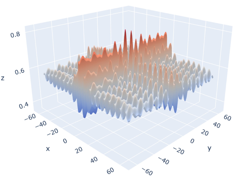
  (a) $\mathtt{Sine}$ FCNN.

  

  (b) $\mathtt{Sine}$ MMNN.

  (c) ${\mathtt{SinTU}}_{0}$ FCNN.

  

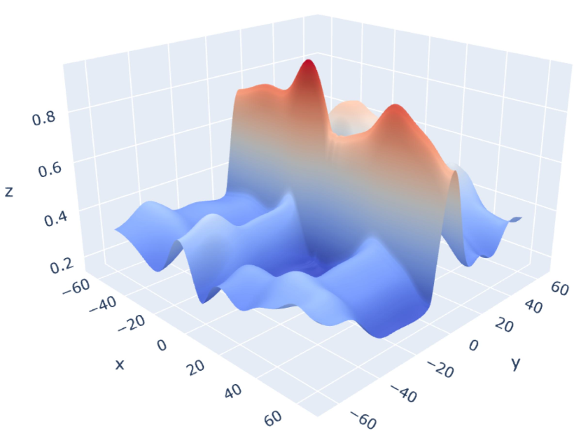
  (d) ${\mathtt{SinTU}}_{0}$ MMNN.

  Figure 1: Comparison of the cost function landscapes in terms of two parameters.

• Finally, extensive numerical experiments demonstrate that Fourier MMNNs (FMMNNs), which use sine or $\mathtt{SinTU}$s as activation functions, consistently outperform other models in both accuracy and efficiency, as shown in Table 1. For $f_{1}$, $\mathtt{sine}$-activated MMNNs achieve the best result, aligning with expectations since $f_{1}$ is $C^{\infty}(\mathbb{R})$ (see Figure 2). The accurate approximation of derivatives is particularly noteworthy, given the complexity of $f_{1}$ and the fact that the training process relies solely on function values, without incorporating derivative information. For $f_{2}\in C^{0}(\mathbb{R})\backslash C^{1}(\mathbb{R})$ (see Figure 2), which contains numerous singularities, ${\mathtt{SinTU}}_{-\pi}$ achieves the best accuracy, demonstrating its effectiveness in capturing these singular features. Notably, even in this inherently challenging case, $\mathtt{sine}$-activated MMNNs still achieve results comparable to the best. For $f_{3}\in C^{0}(\mathbb{R})\backslash C^{1}(\mathbb{R})$ (see Figure 2), FCNNs are highly sensitive to training hyperparameters and often fail with small mini-batches. In contrast, FMMNNs remain stable and perform well across different settings. Even with large mini-batches, training FCNNs is time-consuming, yet they still underperform compared to $\mathtt{sine}$-activated MMNNs. For more details on the experiments, including additional tests in two and three dimensions, refer to Section 3.

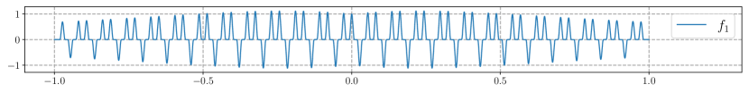
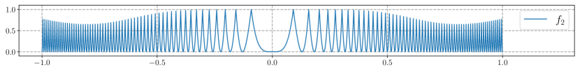
Figure 2: Illustrations of $f_{1}\in C^{\infty}({\mathbb{R}})$ and $f_{2},f_{3}\in C^{0}({\mathbb{R}})\backslash C^{1}({\mathbb{R}})$, defined in (5), (6), and (7).

Table 1: Comparison of test errors. Training is conducted in double precision.

		$\bm{6}$ hidden layers and $\bm{7.3\times 10^{4}}$ trainable parameters
		MMNN		FCNN		#training-samples
target	activation	MSE	MAX	MSE	MAX	mini-batch	all
$f_{1}$	$\mathtt{ReLU}$	$2.24\times 10^{-5}$	$4.06\times 10^{-2}$	$2.31\times 10^{-4}$	$1.93\times 10^{-1}$	3000	3000
$f_{1}$	$\mathtt{tanh}$	$4.91\times 10^{-6}$	$1.24\times 10^{-2}$	$2.67\times 10^{-3}$	$3.69\times 10^{-1}$	3000	3000
$f_{1}$	$\mathtt{sine}$	$\bm{3.43\times 10^{-8}}$	$\bm{8.37\times 10^{-4}}$	$2.62\times 10^{-5}$	$2.35\times 10^{-2}$	3000	3000
$f_{1}$	$\mathtt{SinTU}_{-\pi}$	$3.65\times 10^{-7}$	$4.90\times 10^{-3}$	$4.14\times 10^{-4}$	$1.44\times 10^{-1}$	3000	3000
$f^{\prime}_{1}$	$\mathtt{tanh}$	$1.24\times 10^{-4}$	$5.67\times 10^{-2}$	$1.10\times 10^{-2}$	$6.31\times 10^{-1}$
$f^{\prime}_{1}$	$\mathtt{sine}$	$1.27\times 10^{-6}$	$5.12\times 10^{-3}$	$5.83\times 10^{-4}$	$1.06\times 10^{-1}$
$f^{\prime\prime}_{1}$	$\mathtt{tanh}$	$9.92\times 10^{-4}$	$1.59\times 10^{-1}$	$3.02\times 10^{-2}$	$8.62\times 10^{-1}$
$f^{\prime\prime}_{1}$	$\mathtt{sine}$	$7.82\times 10^{-6}$	$1.37\times 10^{-2}$	$4.45\times 10^{-3}$	$2.71\times 10^{-1}$
$f_{2}$	$\mathtt{ReLU}$	$1.53\times 10^{-3}$	$4.37\times 10^{-1}$	$2.13\times 10^{-2}$	$6.35\times 10^{-1}$	3000	60000
$f_{2}$	$\mathtt{tanh}$	$1.42\times 10^{-4}$	$1.51\times 10^{-1}$	$1.21\times 10^{-2}$	$5.56\times 10^{-1}$	3000	60000
$f_{2}$	$\mathtt{sine}$	$4.84\times 10^{-6}$	$2.88\times 10^{-2}$	$9.07\times 10^{-5}$	$9.22\times 10^{-2}$	3000	60000
$f_{2}$	$\mathtt{SinTU}_{-\pi}$	$\bm{1.28\times 10^{-6}}$	$\bm{2.31\times 10^{-2}}$	$6.14\times 10^{-3}$	$5.31\times 10^{-1}$	3000	60000
$f_{3}$	$\mathtt{sine}$	$7.68\times 10^{-8}$	$6.06\times 10^{-3}$	$3.04\times 10^{-2}$	$6.99\times 10^{-1}$	500	18000
$f_{3}$	$\mathtt{sine}$	$1.27\times 10^{-7}$	$6.58\times 10^{-3}$	$6.69\times 10^{-2}$	$6.68\times 10^{-1}$	1000	18000
$f_{3}$	$\mathtt{sine}$	$8.75\times 10^{-8}$	$6.28\times 10^{-3}$	$2.43\times 10^{-4}$	$1.52\times 10^{-1}$	1500	18000
$f_{3}$	$\mathtt{sine}$	$\bm{6.41\times 10^{-8}}$	$\bm{5.33\times 10^{-3}}$	$5.86\times 10^{-6}$	$3.38\times 10^{-2}$	2000	18000

The paper is structured as follows. Section 2 provides a detailed analysis of the MMNN architecture, demonstrating its strong approximation capabilities when using sine and $\mathtt{SinTU}$s as activation functions. This section also explores key practical aspects, including the cost function landscape and the interaction between sine and MMNNs, highlighting the advantages of keeping weights fixed within activation functions. The section concludes with a discussion of related work. Section 3 presents extensive numerical experiments that support our theoretical findings. Section 4 provides rigorous proofs for the theorems introduced in Section 2, supplemented by several propositions, whose proofs are detailed in Section 5. Finally, Section 6 concludes the paper with a brief discussion.

2 The Potential of the $\mathtt{Sine}$ Activation Function

In this section, we first provide a detailed analysis of the MMNN architecture in Section 2.1, followed by an exploration of its mathematical approximation potential when using sine and $\mathtt{SinTU}$s as activation functions in Section 2.2. In Section 2.3, we examine key practical considerations, including the cost function landscape and the interaction between sine and MMNNs, highlighting the benefits of keeping weights within activation functions fixed. The section concludes with a discussion of related work in Section 2.4.

2.1 Structure of MMNNs

Before presenting the main results, we first introduce the architecture of MMNNs. An MMNN is a multi-layer composition of functions ${\bm{h}}_{i}$, formally defined as ${\bm{h}}:{\mathbb{R}}^{d_{0}}\to{\mathbb{R}}^{d_{m}}$ with

$${\bm{h}}={\bm{h}}_{m}\circ{\bm{h}}_{m-1}\circ\mathinner{\mkern-0.1mu\cdotp\mkern-0.3mu\cdotp\mkern-0.3mu\cdotp\mkern-0.1mu}\circ{\bm{h}}_{1},$$ (1)

where each layer ${\bm{h}}_{i}:{\mathbb{R}}^{d_{i-1}}\to{\mathbb{R}}^{d_{i}}$ represents a multi-component shallow network with width $n_{i}$ and $d_{i}$ components, given by

$${\bm{h}}_{i}({\bm{x}})={\bm{A}}_{i}\,\sigma({\bm{W}}_{i}{\bm{x}}+{\bm{b}}_{i})+{\bm{c}}_{i},$$

where ${\bm{W}}_{i}\in{\mathbb{R}}^{n_{i}\times d_{i-1}}$, ${\bm{b}}_{i}\in{\mathbb{R}}^{n_{i}}$, ${\bm{A}}_{i}\in{\mathbb{R}}^{d_{i}\times n_{i}}$, and ${\bm{c}}_{i}\in{\mathbb{R}}^{d_{i}}$. Here, $\sigma({\bm{W}}_{i}{[j,:]}\cdot{\bm{x}}+{\bm{b}}_{i}[j])$ for $j=1,2,\mathinner{\mkern-0.1mu\cdotp\mkern-0.3mu\cdotp\mkern-0.3mu\cdotp\mkern-0.1mu},n_{i}$ act as randomly parameterized basis functions in ${\mathbb{R}}^{d_{i-1}}$. Each component ${\bm{A}}_{i}[k,:]\sigma({\bm{W}}_{i}{\bm{x}}+{\bm{b}}_{i})+{\bm{c}}_{i}[k]$, for $k=1,2,\mathinner{\mkern-0.1mu\cdotp\mkern-0.3mu\cdotp\mkern-0.3mu\cdotp\mkern-0.1mu},d_{i}$, is a linear combination of these basis functions.

In each layer, the number of components $d_{i-1}$, referred to as rank, is significantly smaller than the number of hidden neurons $n_{i}$, known as the layer width. The utilization of a diverse set of random basis functions, enabled by $n_{i}\gg d_{i-1}$, along with their well-conditioned nature due to random parametrization, facilitates easy training of ${\bm{A}}_{i}$ and ${\bm{c}}_{i}$ to approximate smooth functions in ${\mathbb{R}}^{d_{i-1}}$. By integrating multiple components per layer and composing multiple layers, this balance between rank and width, combined with the flexible component structure employing random bases, enhances the effectiveness of MMNNs in both representation and learning. The width of an MMNN is defined as $\max\{n_{i}:i=1,2,\mathinner{\mkern-0.1mu\cdotp\mkern-0.3mu\cdotp\mkern-0.3mu\cdotp\mkern-0.1mu},m-1\}$, the rank as $\max\{d_{i}:i=1,2,\mathinner{\mkern-0.1mu\cdotp\mkern-0.3mu\cdotp\mkern-0.3mu\cdotp\mkern-0.1mu},m-1\}$, and the depth as $m$. For convenience, we use the compact notation $(N,R,L)$ to denote a network of width $N$, rank $R$, and depth $L$. In most of our experiments, we assume equal layer width and rank, i.e., $n_{i}=N$ and $d_{i}=R$.

In summary, MMNNs consider each component as a fundamental unit, where it consists of a linear combination of randomly parameterized neurons (basis functions). This contrasts with FCNNs, which treat individual neurons as the primary units. Components within each layer are combined and further composed across layers to effectively approximate target functions. The MMNN structure is enriched by introducing rank as an additional dimension alongside width and depth, offering greater flexibility in network architecture. Furthermore, the training paradigm for MMNNs diverges significantly from that of FCNNs. Within each MMNN layer, represented by ${\bm{A}}\,\sigma({\bm{W}}{\bm{x}}+{\bm{b}})+{\bm{c}}$, the set

$$\big{\{}\sigma({\bm{W}}{[j,:]}\cdot{\bm{x}}+{\bm{b}}[j]):j=1,2,\mathinner{\mkern-0.1mu\cdotp\mkern-0.3mu\cdotp\mkern-0.3mu\cdotp\mkern-0.1mu},n\big{\}}$$

is interpreted as a shared random basis for all components. Consequently, during training, only the parameters ${\bm{A}}$ and ${\bm{c}}$ are updated, while ${\bm{W}}$ and ${\bm{b}}$ remain fixed after random initialization.

To mitigate the vanishing gradient issue in deep MMNNs, techniques inspired by ResNets (He et al., 2016) can be employed to improve training efficiency. Building on this concept, we introduce the ResMMNN, which modifies the structure of (1) as

$${\bm{h}}={\bm{h}}_{m}\circ({\bm{I}}+{\bm{h}}_{m-1})\circ\mathinner{\mkern-0.1mu\cdotp\mkern-0.3mu\cdotp\mkern-0.3mu\cdotp\mkern-0.1mu}\circ({\bm{I}}+{\bm{h}}_{3})\circ({\bm{I}}+{\bm{h}}_{2})\circ{\bm{h}}_{1},$$

where ${\bm{I}}$ denotes the identity mapping. This definition of ResMMNN can be further generalized by applying identity mappings selectively to specific layers. Such variations are still referred to as ResMMNNs. See Figure 3 for an illustration of a ResMMNN with size $(6,2,3)$. Furthermore, additional layer operations, such as Batch Normalization (Ioffe and Szegedy, 2015) and Dropout (Srivastava et al., 2014), can also be applied to specific layers of MMNNs to enhance training stability, accelerate convergence, and improve generalization, among other benefits.

Figure 3: An illustration of a ResMMNN of size $(6,2,3)$. During training, only the parameters ${\bm{A}}_{i}$’s and ${\bm{c}}_{i}$’s are updated, while ${\bm{W}}_{i}$’s and ${\bm{b}}_{i}$’s are randomly initialized and remain fixed.

2.2 Approximation Capability

We first introduce some notations before presenting our main results on the exponential approximation capabilities of MMNNs using sine or $\mathtt{SinTU}$s as activation functions. We denote ${\hskip 0.6pt\mathcal{M}\hskip 0.0pt\mathcal{N}\hskip-0.8pt}_{\varrho}\{N,\hskip 2.2ptR,\hskip 2.2ptL;\hskip 3.0297pt{{\mathbb{R}}^{d}}\hskip-1.0298pt\to\hskip-0.98pt{{\mathbb{R}}^{n}}\}$ as the set of vector-valued functions ${\bm{\phi}}:\mathbb{R}^{d}\to\mathbb{R}^{n}$ that can be represented by $\varrho$-activated MMNNs of width $\leq N\in{\mathbb{N}}^{+}$, rank $\leq R\in{\mathbb{N}}^{+}$, and depth $\leq L\in{\mathbb{N}}^{+}$. Additionally, in this notation, if $\varrho$ is replaced by $(\varrho_{1},\mathinner{\mkern-0.1mu\cdotp\mkern-0.3mu\cdotp\mkern-0.3mu\cdotp\mkern-0.1mu},\varrho_{k})$, it indicates that each neuron can be activated by any of $\varrho_{i}$’s. Let $\omega_{f}(\cdot)$ be the modulus of continuity of $f\in C([0,1]^{d})$ defined via

$$\omega_{f}(t)\coloneqq\sup\big{\{}|f({\bm{x}})-f({\bm{y}})|:\|{\bm{x}}-{\bm{y}}\|_{2}\leq t,\,\;{\bm{x}},{\bm{y}}\in[0,1]^{d}\big{\}}\quad\textnormal{for any $t\geq 0$.}$$

Let ${\mathcal{S}}$ denote the set of $\mathtt{SinTU}$s, i.e.,

$${\mathcal{S}}\coloneqq\{{\mathtt{SinTU}}_{s}:s\in{\mathbb{R}}\}\quad\textnormal{where}\quad{\mathtt{SinTU}}_{s}\coloneqq\sin\circ{\mathcal{T}}_{s}\quad\textnormal{and}\quad{\mathcal{T}}_{s}(x)\coloneqq\max\{x,\,s\}=\begin{cases}x&\text{if }x\geq s,\\ s&\text{if }x<s.\end{cases}$$

With the above notations, we present the following theorem, which demonstrates that MMNNs activated by $\mathtt{SinTU}$s possess exponential approximation power.

Theorem 2.1.

Given $f\in C([0,1]^{d})$ and $\varrho\in{\mathcal{S}}$, for any $N,L\in\mathbb{N}^{+}$ and $p\in[1,\infty)$, there exists $\phi\in{\hskip 0.6pt\mathcal{M}\hskip 0.0pt\mathcal{N}\hskip-0.8pt}_{\varrho}\big{\{}2d(4N-1),\hskip 2.2pt3d,\hskip 2.2ptL+2;\hskip 3.0297pt{\mathbb{R}^{d}}\hskip-1.0298pt\to\hskip-0.98pt{\mathbb{R}}\big{\}}$ such that

$$\|\phi-f\|_{L^{p}([0,1]^{d})}\leq 2\sqrt{d}\cdot\omega_{f}\big{(}N^{-L}\big{)}.$$

The preceding theorem establishes the approximation capabilities of MMNNs activated by $\mathtt{SinTU}$s, which are truncated variations of the $\mathtt{sine}$ function. Next, we explore the case where the pure $\mathtt{sine}$ function is used as the activation function. However, due to its lack of singularity, the $\mathtt{sine}$ function poses challenges in spatial localization, making it difficult to construct mathematical frameworks for spatial decomposition based on continuity. To overcome this mathematical challenge, we introduce $\mathtt{ReLU}$ as an additional activation function. This modification enables a more effective spatial decomposition, leading to the following theorem.

Theorem 2.2.

Given $f\in C([0,1]^{d})$, for any $N,L\in\mathbb{N}^{+}$ and $p\in[1,\infty)$, there exist $\phi\in{\hskip 0.6pt\mathcal{M}\hskip 0.0pt\mathcal{N}\hskip-0.8pt}_{({\mathtt{sine}},\,{\mathtt{ReLU}})}\big{\{}d(4N-1),\hskip 2.2pt3d,\hskip 2.2ptL+2;\hskip 3.0297pt{\mathbb{R}^{d}}\hskip-1.0298pt\to\hskip-0.98pt{\mathbb{R}}\big{\}}$ such that

$$\|\phi-f\|_{L^{p}([0,1]^{d})}\leq 2\sqrt{d}\cdot\omega_{f}\big{(}N^{-L}\big{)}.$$

Remark 2.3.

The theorem does not impose a specific arrangement of ${\mathtt{sine}}$ and $\mathtt{ReLU}$. However, our proof demonstrates that applying $\mathtt{ReLU}$ to all but the last two hidden layers, where ${\mathtt{sine}}$ is used, is sufficient. This result is theoretical; in practice, additional ${\mathtt{sine}}$ activation functions may be required, as discussed later.

We adopt a notation for FCNNs analogous to ${\hskip 0.6pt\mathcal{M}\hskip 0.0pt\mathcal{N}\hskip-0.8pt}_{\varrho}\{N,\hskip 2.2ptR,\hskip 2.2ptL;\hskip 3.0297pt{{\mathbb{R}}^{d}}\hskip-1.0298pt\to\hskip-0.98pt{{\mathbb{R}}^{n}}\}$ used for MMNNs. Specifically, let ${\hskip 0.6pt\mathcal{F}\hskip-0.828pt\mathcal{N}\hskip-0.725pt}_{\varrho}\{N,\hskip 1.987ptL;\hskip 3.0297pt{{\mathbb{R}}^{d}}\hskip-1.0298pt\to\hskip-0.98pt{{\mathbb{R}}^{n}}\}$ denote the set of vector-valued functions ${\bm{\phi}}:\mathbb{R}^{d}\to\mathbb{R}^{n}$ that can be realized by $\varrho$-activated FCNNs with width at most $N\in\mathbb{N}^{+}$ and depth at most $L\in\mathbb{N}^{+}$. Similarly, if $\varrho$ is replaced by $(\varrho_{1},\mathinner{\mkern-0.1mu\cdotp\mkern-0.3mu\cdotp\mkern-0.3mu\cdotp\mkern-0.1mu},\varrho_{k})$, it indicates that each neuron can be activated by any of the $\varrho_{i}$’s. As a direct consequence of Theorems 2.1 and 2.2, we establish the following two corollaries for FCNNs.

Corollary 2.4.

Given $f\in C([0,1]^{d})$ and $\varrho\in{\mathcal{S}}$, for any $N,L\in\mathbb{N}^{+}$ and $p\in[1,\infty)$, there exists $\phi\in{\hskip 0.6pt\mathcal{F}\hskip-0.828pt\mathcal{N}\hskip-0.725pt}_{\varrho}\big{\{}2d(4N-1),\hskip 1.987ptL+2;\hskip 3.0297pt{\mathbb{R}^{d}}\hskip-1.0298pt\to\hskip-0.98pt{\mathbb{R}}\big{\}}$ such that

$$\|\phi-f\|_{L^{p}([0,1]^{d})}\leq 2\sqrt{d}\cdot\omega_{f}\big{(}N^{-L}\big{)}.$$

Corollary 2.5.

Given $f\in C([0,1]^{d})$, for any $N,L\in\mathbb{N}^{+}$ and $p\in[1,\infty)$, there exist $\phi\in{\hskip 0.6pt\mathcal{F}\hskip-0.828pt\mathcal{N}\hskip-0.725pt}_{(\sin,\,{\mathtt{ReLU}})}\big{\{}d(4N-1),\hskip 1.987ptL+2;\hskip 3.0297pt{\mathbb{R}^{d}}\hskip-1.0298pt\to\hskip-0.98pt{\mathbb{R}}\big{\}}$ such that

$$\|\phi-f\|_{L^{p}([0,1]^{d})}\leq 2\sqrt{d}\cdot\omega_{f}\big{(}N^{-L}\big{)}.$$

Remark 2.6.

It is worth highlighting the substantial difference in the total number of parameters between an MMNN and an FCNN. For an MMNN of width $N$, rank $R$, and depth $L$, the parameter count is $O(NRL)$, whereas for an FCNN of width $N$ and depth $L$, it is $O(N^{2}L)$. Notably, in an MMNN, the rank $R$ (the number of components in each layer) is significantly smaller than the network width $N$ (the number of random hidden neurons per layer), which guarantees that the set of $N$ random basis is diverse enough to approximate smooth functions in the input space of dimension $R$ from the previous layer. Additionally, as previously discussed, only half of the parameters in an MMNN are trained.

Remark 2.7.

By applying techniques from (Lu et al., 2021) (specifically Theorem 2.1), the above results could be extended to the $L^{\infty}$-norm, although the constants involved would be considerably larger. The extension involves more technical complexities and is of little importance to the main themes of this paper, so we do not pursue it here.

The proofs of Theorems 2.1 and 2.2 (see Section 4) rely on two key components. The first component involves constructing a subnetwork that partitions a $d$-dimensional unit hypercube into uniform subcubes of small size, with only a minor discrepancy due to the continuity of the activation function. Within each subcube, the function is approximated by a constant function. The second component is the existence of a subnetwork that maps the index of each subcube to the function value at a representative point within the subcube (e.g., its center). In designing this subnetwork, it suffices to ensure accuracy at a finite set of points rather than over an entire interval. This highlights the power of composition, which simplifies the construction. As we shall see later, the periodicity and irrationality of the sine function play a crucial role in efficiently addressing the second component. Specifically, for any $\varepsilon>0$ and any $M\in\mathbb{N}^{+}$, given $f_{n}\in[-1,1]$, there exist suitable values of $v$ and $w$ such that

$$\left|\sin\big{(}v\cdot\sin(nw)\big{)}-f_{n}\right|<\varepsilon\quad\text{for }n=1,2,\mathinner{\mkern-0.1mu\cdotp\mkern-0.3mu\cdotp\mkern-0.3mu\cdotp\mkern-0.1mu},M.$$ (2)

Although many mathematical approximation results show theoretical representation power, however, in practice, a more important issue is whether one has an efficient training strategy to achieve a good computational performance. For most mathematical neural network approximation results (constructive or non-constructive), the network parameters depends on target function nonlinearly and globally. On the other hand, most training processes are gradient descent based (first order) methods which are very local and sensitive to ill-conditioning of the cost function in terms of a very large number of parameters. This typically leads to a gap between the theoretical results and practical performance. In our case, although two $\mathtt{sine}$ functions (or $\mathtt{SinTU}$s) are theoretically sufficient for value fitting (e.g., Equation (2)), finding the two appropriate numbers, $v$ and $w$, is non-practical in general. Consequently, a larger network with multiple components and layers is essential for effective optimization.

Mathematical and numerical investigations in later sections demonstrate that using sine or $\mathtt{SinTU}$s as activation functions in MMNNs with well balanced structures, significantly improves the network’s capability and learning efficiency. This is consistent with the key feature of MMNNs that each component, which is a one hidden layer network, only needs to approximate a smooth function and can be trained effectively while Fourier series can approximate smooth functions efficiently.

2.3 Optimization Landscapes

In Section 2.2, we demonstrate that MMNNs activated by sine or $\mathtt{SinTU}$s possess strong approximation capabilities. However, having good approximation power only reflects theoretical potential and does not necessarily guarantee effective learning in practice. Next, we discuss the practical learning difficulty of MMNNs activated by sine or $\mathtt{SinTU}$s. We focus on the most intuitive aspect: the landscape of the cost function with respect to the network parameters, which serves as an indicator of the training complexity in practice. This analysis is conducted across various network architectures and activation functions.

We first consider three basic cases where the target function $f$ takes the following forms:

$$\sin(w^{*}x+b^{*}),\quad\sum_{i=1}^{2}\sin(w_{i}^{*}x),\quad\text{and}\quad\sin\big{(}w_{2}^{*}\sin(w_{1}^{*}x)\big{)},$$

respectively. The corresponding cost functions are given by

$$\mathcal{L}_{1}(w_{1},w_{2})=\int_{-\pi}^{\pi}\Big{(}\sin(w_{1}x+w_{2})-\sin(w_{1}^{*}x+w_{2}^{*})\Big{)}^{2}\,dx,$$

$$\mathcal{L}_{2}(w_{1},w_{2})=\int_{-\pi}^{\pi}\Bigg{(}\sum_{i=1}^{2}\sin(w_{i}x)-\sum_{i=1}^{2}\sin(w_{i}^{*}x)\Bigg{)}^{2}\,dx,$$

and

$$\mathcal{L}_{3}(w_{1},w_{2})=\int_{-\pi}^{\pi}\Big{(}\sin\big{(}w_{2}\sin(w_{1}x)\big{)}-\sin\big{(}w_{2}^{*}\sin(w_{1}^{*}x)\big{)}\Big{)}^{2}\,dx.$$

(a) ${\mathcal{L}}_{1}(w_{1},w_{2})$.

(b) ${\mathcal{L}}_{2}(w_{1},w_{2})$.

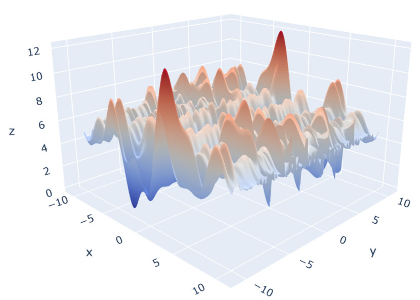
(c) ${\mathcal{L}}_{3}(w_{1},w_{2})$.

Figure 4: Landscape visualizations of $\mathcal{L}_{i}$ for $i=1,2,3$, where $x$, $y$, and $z$ represent $w_{1}$, $w_{2}$, and $\mathcal{L}_{i}(w_{1},w_{2})$, respectively.

Here, we use the integration range $(-\pi,\pi)$ instead of $(-1,1)$ because the $\mathtt{sine}$ function has a period of $2\pi$, which simplifies the calculations and makes the test more straightforward. The landscapes of these three cost functions are illustrated in Figure 4. As observed, the landscapes are quite complex, featuring numerous local minima. This indicates that using the $\mathtt{sine}$ function as an activation function poses significant challenges for effective learning in practice. We will later see that this issue is particularly severe for FCNNs. However, the structure of MMNNs simplifies the landscape, making them more conducive to effective learning.

Next, we examine general network architectures, specifically FMMNNs and FCNNs. To ensure a fair comparison, the FCNN is designed to have a comparable number of learnable parameters to the MMNN. The FCNN is defined as

$$\phi(x)=\mathcal{A}_{2}\circ\varrho\circ{\mathcal{A}}_{1}\circ\varrho\circ{\mathcal{A}}_{0}(x),$$ (3)

where ${\mathcal{A}}_{0}:\mathbb{R}\to\mathbb{R}^{64}$, ${\mathcal{A}}_{1}:\mathbb{R}^{64}\to\mathbb{R}^{64}$, $\mathcal{A}_{2}:\mathbb{R}^{64}\to\mathbb{R}$ are affine linear maps, and $\varrho$ is either the $\mathtt{sine}$ or ${\mathtt{SinTU}}_{0}$ activation function. The MMNN is defined as

$$\phi(x)=\widetilde{\mathcal{A}}_{3}\circ\varrho\circ{\widetilde{\mathcal{A}}}_{2}\circ{\widetilde{\mathcal{A}}}_{1}\circ\varrho\circ{\widetilde{\mathcal{A}}}_{0}(x),$$ (4)

where ${\widetilde{\mathcal{A}}}_{0}:\mathbb{R}\to\mathbb{R}^{128}$, ${\widetilde{\mathcal{A}}}_{1}:\mathbb{R}^{128}\to\mathbb{R}^{32}$, ${\widetilde{\mathcal{A}}}_{2}:\mathbb{R}^{32}\to\mathbb{R}^{128}$, $\widetilde{\mathcal{A}}_{3}:\mathbb{R}^{128}\to\mathbb{R}$ are affine linear maps. The cost function is given by

$${\mathcal{L}}(w_{1},w_{2})=\int_{-\pi}^{\pi}\Big{(}\phi(x)-f(x)\Big{)}^{2}\,dx,\quad\textnormal{where}\quad f(x)=\frac{1}{1+100x^{2}}.$$

As shown in (a), (b), (d), and (e) of Figure 5, the learning landscape of MMNNs is considerably simpler than that of FCNNs. Likewise, (b), (c), (e), and (f) of Figure 5 clearly illustrate that our learning strategy, which involves fixing parameters in ${\mathcal{\widetilde{A}}}_{2}$ while optimizing those in ${\mathcal{\widetilde{A}}}_{1}$ rather than the reverse, is well-justified and reasonable. We would like to point out that different initializations can produce varying results; however, the overall landscape complexity remains largely consistent. The figures shown in Figure 5 represent relatively complex cases among several initializations with identical settings. We have experimented with deeper networks and other target functions, and the results are generally similar to the two-hidden-layer cases presented. For deeper MMNNs, if two parameters are selected from the trainable parameters (i.e., ${\bm{A}}_{i}$’s and ${\bm{c}}_{i}$’s, see Section 2.1), the landscape always remains simple, reflecting the effectiveness and rationality of our training strategy.

(a) FCNN (${\mathcal{A}}_{1}$ in (3)).

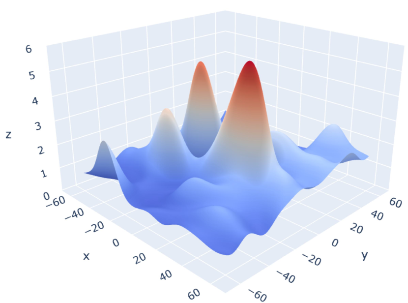
(b) MMNN (${\mathcal{\widetilde{A}}}_{1}$ in (4)).

(c) MMNN (${\mathcal{\widetilde{A}}}_{2}$ in (4)).

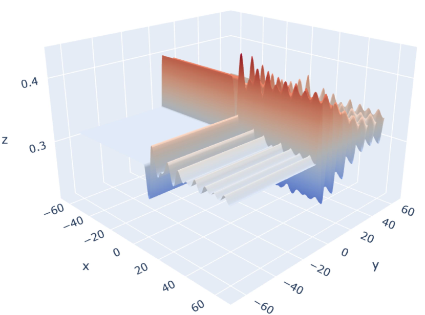
(d) FCNN (${\mathcal{A}}_{1}$ in (3)).

(e) MMNN (${\mathcal{\widetilde{A}}}_{1}$ in (4)).

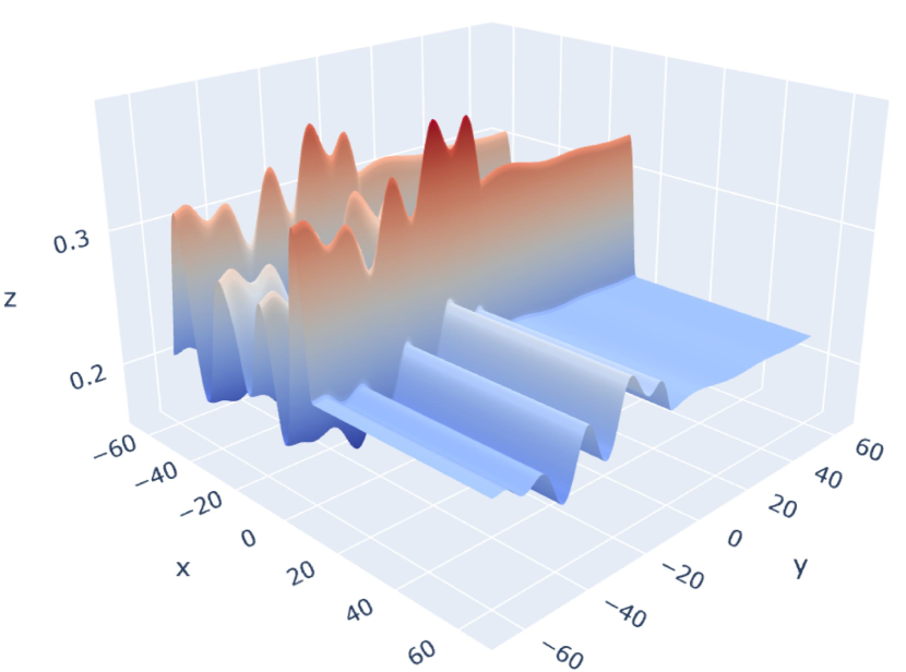
(f) MMNN (${\mathcal{\widetilde{A}}}_{2}$ in (4)).

Figure 5: Comparison of the cost function landscapes for FCNNs and MMNNs. All parameters are initialized using PyTorch’s default linear initialization. Here, $z$ represents the cost function, while $x$ and $y$ denote two parameters from the weights of ${\mathcal{A}}_{1}$, ${\widetilde{\mathcal{A}}}_{1}$, and ${\widetilde{\mathcal{A}}}_{2}$ in (3) and (4). The top and bottom rows correspond to the $\mathtt{sine}$ and ${\mathtt{SinTU}}_{0}$ activation functions, respectively.

2.4 Related Work

Extensive research has explored the approximation capabilities of neural networks across various architectures. Early works established the universal approximation theorem for single-hidden-layer networks (Cybenko, 1989; Hornik, 1991; Hornik et al., 1989), proving their ability to approximate specific functions arbitrarily well, though without quantifying error in relation to network size. Subsequent studies (Yarotsky, 2018, 2017; Bölcskei et al., 2019; Zhou, 2020; Chui et al., 2018; Gribonval et al., 2022; Gühring et al., 2020; Montanelli and Yang, 2020; Shen et al., 2019, 2020; Lu et al., 2021; Shen et al., 2022a; Zhang, 2020; Shen et al., 2022b; Zhang et al., 2024a; Yarotsky and Zhevnerchuk, 2020; Fang and Xu, 2024; Zhang et al., 2024a) analyzed approximation errors, relating them to network width, depth, or parameter count, and addressed the spectral bias in neural network approximations. Here, we specifically highlight two papers (Shen et al., 2022a; Yarotsky and Zhevnerchuk, 2020) that are closely related to our theoretical results. The results in (Yarotsky and Zhevnerchuk, 2020) imply that $\mathtt{ReLU}$/$\mathtt{sine}$-activated fully connected neural networks (FCNNs) with width $O(d)$ and depth $O(L)$ can approximate a 1-Lipschitz function $f:[0,1]^{d}\to\mathbb{R}$ within an error of $O(2^{-\sqrt{L}})$. Compared to this, our work achieves several key improvements: 1) Our results incorporate width $N$, extending beyond fixed-width networks. 2) We improve the approximation error rate to $O(N^{-L})$, much better than $O(2^{-\sqrt{L}})$ when $N$ fixed. 3) We introduce $\mathtt{SinTU}$, a novel hybrid activation function, where a single $\mathtt{SinTU}$ function can replace two activation functions ($\mathtt{ReLU}$, $\mathtt{sine}$) in the approximation results. 4) Our results specifically apply to MMNNs, which introduce an additional dimension called rank beyond width and depth. In (Shen et al., 2022a), the author proposes a simple activation function, $\mathtt{EUAF}$, and demonstrates that a fixed-size $\mathtt{EUAF}$-activated FCNN can approximate any continuous function $f\in C([0,1]^{d})$ to an arbitrarily small error by adjusting only finitely many parameters. $\mathtt{EUAF}$ emphasizes theoretical approximation but tends to perform less effectively in practice, often appearing somewhat artificial. In contrast, our FMMNN is naturally structured. Although its theoretical approximation power is comparatively weaker, an exponential approximation rate is typically sufficient in practical applications. Our extensive experiments further confirm its effectiveness, demonstrating surprisingly strong empirical performance.

Some previous works have explored the use of $\mathtt{sine}$ as an activation function in multi-layer networks (Cai et al., 2020; Novello et al., 2024; Morsali et al., 2025; Fathony et al., 2021; Jiao et al., 2023; Sitzmann et al., 2020). The authors in (Novello et al., 2024; Morsali et al., 2025) present numerical examples demonstrating the advantages of sine-activated networks, primarily in FCNNs. Additionally, (Fathony et al., 2021) introduces a multiplicative filter network that incorporates sinusoidal filters and illustrates its benefits through various examples. To the best of our knowledge, existing works do not provide strong mathematical or numerical justification for the benefits of sine, which is a key reason why it is rarely used in practice. This paper first establishes rigorous approximation results, followed by an intuitive landscape analysis of the cost function to assess learning potential, and finally validates these findings through extensive numerical experiments. Our experiments show that using the sine activation in FCNNs does not always lead to good performance. While it works well in some cases, it performs quite poorly in others. We believe this inconsistency is the main reason why sine is not widely adopted in practice. Surprisingly, we found that our MMNN network structure and sine (or $\mathtt{SinTU}$s) form a highly effective combination. Compared to FCNNs, MMNNs exhibit a simpler optimization landscape. Our experiments confirm this observation, as MMNNs achieve consistently strong performance across all test cases.

3 Numerical Experiments

In this section, we conduct extensive experiments to validate our analysis and demonstrate the effectiveness of MMNNs. Across all tests, we ensure: (1) sufficient data sampling to capture fine details of the target function, (2) the use of the Adam optimizer (Kingma and Ba, 2015) for training, (3) mean squared error (MSE) as the training loss function, with both MSE and MAX ($L^{\infty}$-norm) used for evaluation, (4) parameter initialization following PyTorch’s default settings, (5) fixed ${\bm{W}}$ and ${\bm{b}}$ (parameters inside activation functions), while only ${\bm{A}}$ and ${\bm{c}}$ (parameters outside activation functions) are trained (see Section 2.1 for details).

Section 3.1 compares MMNNs and FCNNs across various activation functions, including $\mathtt{ReLU}$, $\mathtt{GELU}$, tanh, sine, $\mathtt{cosine}$, and $\mathtt{SinTU}$s. Section 3.2 focuses on MMNNs, analyzing the performance of sine relative to other activation functions.

3.1 MMNNs Versus FCNNs

We will thoroughly compare the performance of MMNNs and FCNNs using various activation functions. The overall message from these tests is that: 1) MMNNs perform better than FCNNs when the same activation function is used, and 2) FMMNNs always produce the best results. In our tests, we select rather complex target functions – highly oscillatory with or without non-smoothness, as both network types perform well on simple functions, making their differences less apparent. Additionally, our target functions should not be generated using $\mathtt{sine}$, $\mathtt{cosine}$, or their compositions and combinations, since we use $\mathtt{sine}$ as the activation function. Based on these considerations, we first choose an oscillatory target function $f_{1}\in C^{\infty}({\mathbb{R}})$ defined as

$$f_{1}(x)=\frac{1}{1+2x^{2}}\sum_{i=-n}^{n}(-1)^{(i\bmod 3)}\cdot\frac{|i|+n}{n}\cdot g\left((2n+1)\left(x-\frac{i}{n+1}\right)\right),\\$$ (5)

where $n=36$, and $(i\bmod 3)\in\{0,1,2\}$ represents the remainder when an integer $i\in{\mathbb{Z}}$ is divided by 3. Here, $g$ serves as a basis function, defined as

$$g(x)=\frac{g_{0}(x+1)g_{0}(1-x)}{g_{0}^{2}(1)},\quad\textnormal{where}\quad g_{0}(x)=\begin{cases}\exp\left(-\frac{1}{x^{2}}\right)&\textnormal{if}\ x>0,\\ 0&\textnormal{if}\ x\leq 0.\end{cases}$$

It is easy to verify that $g_{0}\in C^{\infty}(\mathbb{R})$, and hence $f\in C^{\infty}(\mathbb{R})$. See Figure 6 for illustrations of $f_{1}$ and $g$. Next, we choose two non-smooth oscillatory functions $f_{2},f_{3}\in C^{0}({\mathbb{R}})\backslash C^{1}({\mathbb{R}})$ given by

$$f_{2}(x)=\frac{1+6x^{8}}{1+8x^{6}}\cdot\left(120x^{2}-2\left\lfloor\frac{120x^{2}+1}{2}\right\rfloor\right)^{2}$$ (6)

and

$$f_{3}(x)=\frac{1+6x^{8}}{1+8x^{6}}\cdot\left(32x-2\left\lfloor\frac{32x+1}{2}\right\rfloor\right)^{2},$$ (7)

where $\lfloor\cdot\rfloor$ denotes the floor function. See Figure 6 for visual depictions of $f_{2}$ and $f_{3}$. For $f_{3}$, we use different mini-batch size to demonstrate that MMNNs are less sensitive to the hyper-parameters of training and therefore more stable compared to FCNNs.

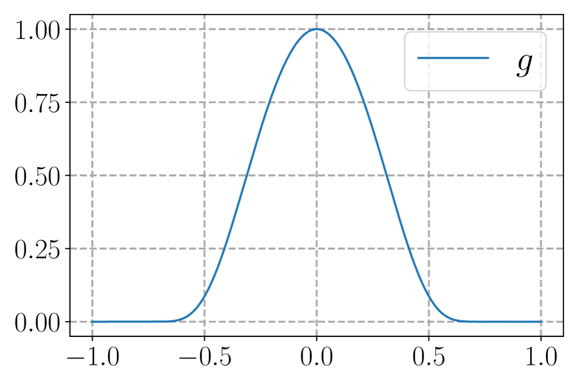
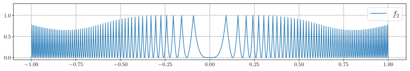
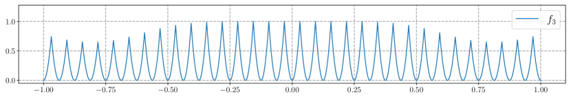
Figure 6: Illustrations of $f_{1}$, $g$, $f_{2}$, and $f_{3}$.

We employ various network architectures to approximate these functions and evaluate their performance. Notably, these tests are conducted using double precision rather than the default single precision to ensure precise comparisons. For the test corresponding to $f_{1}$, we use a total of 3000 uniformly sampled points from $[-1,1]$ for training. The mini-batch size is set to 3000, meaning all samples are trained simultaneously. The learning rate is defined as $10^{-3}\times 0.9^{\lfloor k/3000\rfloor}$, where $k=1,2,\mathinner{\mkern-0.1mu\cdotp\mkern-0.3mu\cdotp\mkern-0.3mu\cdotp\mkern-0.1mu},300000$ denotes the epoch number. For the test error evaluation, we use another set of 3,000 samples drawn from the uniform distribution $\mathcal{U}(-1,1)$. We emphasize that the mini-batch method is not used for $f_{1}$ because our tests indicate that while mini-batching preserves the approximation of the original function, it leads to poor derivative approximation by only including function values in the cost function. As we can see from Table 2, $\mathtt{sine}$-activated MMNNs perform best as the target function $f_{1}$ is smooth. We point out that the errors for derivatives in Table 2 are relative errors, as absolute errors for derivatives can be misleading (the $L^{\infty}$-norm of $f_{1}^{\prime\prime}$ exceeds 70,000). The accurate approximation of derivatives is surprising, given the complexity of the target function and the fact that the cost function is formulated solely based on the function values, meaning that no information about $f_{1}^{\prime}$ or $f_{1}^{\prime\prime}$ is incorporated into the optimization process.

Table 2: Comparison of test errors. Training is conducted in double precision, with the cost function relying only on function values and excluding derivatives. Relative errors are reported for derivatives, as the $L^{\infty}$-norm of $f_{1}^{\prime\prime}$ exceeds 70000, making absolute errors misleading.

#parameters (trained / all)		35235 / 72993		72981 / 151281		72961 / 72961
		MMNN of size (434,16,6)		MMNN of size (900,16,6)		FCNN of size (120,–,6)		#training-samples
target function	activation	MSE	MAX	MSE	MAX	MSE	MAX	mini-batch	all
$f_{1}$	$\mathtt{ReLU}$	$4.47\times 10^{-5}$	$6.34\times 10^{-2}$	$2.24\times 10^{-5}$	$4.06\times 10^{-2}$	$2.31\times 10^{-4}$	$1.93\times 10^{-1}$	3000	3000
$f_{1}$	$\mathtt{GELU}$	$5.54\times 10^{-5}$	$5.94\times 10^{-2}$	$1.45\times 10^{-4}$	$1.00\times 10^{-1}$	$1.63\times 10^{-3}$	$2.91\times 10^{-1}$	3000	3000
$f_{1}$	$\mathtt{tanh}$	$4.12\times 10^{-5}$	$2.90\times 10^{-2}$	$4.91\times 10^{-6}$	$1.24\times 10^{-2}$	$2.67\times 10^{-3}$	$3.69\times 10^{-1}$	3000	3000
$f_{1}$	$\mathtt{sine}$	$7.30\times 10^{-7}$	$3.69\times 10^{-3}$	$\bm{3.43\times 10^{-8}}$	$\bm{8.37\times 10^{-4}}$	$2.62\times 10^{-5}$	$2.35\times 10^{-2}$	3000	3000
$f_{1}$	$\mathtt{cosine}$	$6.89\times 10^{-6}$	$9.54\times 10^{-3}$	$1.35\times 10^{-7}$	$1.85\times 10^{-3}$	$2.80\times 10^{-6}$	$7.76\times 10^{-3}$	3000	3000
$f_{1}$	$\mathtt{SinTU}_{0}$	$8.11\times 10^{-5}$	$8.65\times 10^{-2}$	$4.40\times 10^{-6}$	$1.81\times 10^{-2}$	$2.15\times 10^{-4}$	$1.52\times 10^{-1}$	3000	3000
$f_{1}$	$\mathtt{SinTU}_{-\pi}$	$1.25\times 10^{-5}$	$2.76\times 10^{-2}$	$3.65\times 10^{-7}$	$4.90\times 10^{-3}$	$4.14\times 10^{-4}$	$1.44\times 10^{-1}$	3000	3000
$f_{1}$	$\mathtt{SinTU}_{-2\pi}$	$4.19\times 10^{-6}$	$1.30\times 10^{-2}$	$3.97\times 10^{-7}$	$4.93\times 10^{-3}$	$1.67\times 10^{-5}$	$2.63\times 10^{-2}$	3000	3000
$f^{\prime}_{1}$	$\mathtt{GELU}$	$1.24\times 10^{-3}$	$2.61\times 10^{-1}$	$2.34\times 10^{-3}$	$2.97\times 10^{-1}$	$7.74\times 10^{-3}$	$5.16\times 10^{-1}$
$f^{\prime}_{1}$	$\mathtt{tanh}$	$7.50\times 10^{-4}$	$1.11\times 10^{-1}$	$1.24\times 10^{-4}$	$5.67\times 10^{-2}$	$1.10\times 10^{-2}$	$6.31\times 10^{-1}$
$f^{\prime}_{1}$	$\mathtt{sine}$	$2.64\times 10^{-5}$	$2.12\times 10^{-2}$	$\bm{1.27\times 10^{-6}}$	$\bm{5.12\times 10^{-3}}$	$5.83\times 10^{-4}$	$1.06\times 10^{-1}$
$f^{\prime}_{1}$	$\mathtt{cosine}$	$1.77\times 10^{-4}$	$4.76\times 10^{-2}$	$5.35\times 10^{-6}$	$1.15\times 10^{-2}$	$8.91\times 10^{-5}$	$3.84\times 10^{-2}$
$f^{\prime\prime}_{1}$	$\mathtt{GELU}$	$1.03\times 10^{-2}$	$1.22\times 10^{0}$	$1.55\times 10^{-2}$	$9.39\times 10^{-1}$	$3.10\times 10^{-2}$	$1.39\times 10^{0}$
$f^{\prime\prime}_{1}$	$\mathtt{tanh}$	$5.40\times 10^{-3}$	$2.79\times 10^{-1}$	$9.92\times 10^{-4}$	$1.59\times 10^{-1}$	$3.02\times 10^{-2}$	$8.62\times 10^{-1}$
$f^{\prime\prime}_{1}$	$\mathtt{sine}$	$2.32\times 10^{-4}$	$7.40\times 10^{-2}$	$\bm{7.82\times 10^{-6}}$	$\bm{1.37\times 10^{-2}}$	$4.45\times 10^{-3}$	$2.71\times 10^{-1}$
$f^{\prime\prime}_{1}$	$\mathtt{cosine}$	$1.48\times 10^{-3}$	$1.30\times 10^{-1}$	$4.12\times 10^{-5}$	$5.98\times 10^{-2}$	$7.87\times 10^{-4}$	$1.15\times 10^{-1}$
$f_{2}$	$\mathtt{ReLU}$	$4.15\times 10^{-3}$	$4.87\times 10^{-1}$	$1.53\times 10^{-3}$	$4.37\times 10^{-1}$	$2.13\times 10^{-2}$	$6.35\times 10^{-1}$	3000	60000
$f_{2}$	$\mathtt{GELU}$	$4.15\times 10^{-3}$	$4.72\times 10^{-1}$	$1.24\times 10^{-3}$	$4.15\times 10^{-1}$	$1.33\times 10^{-2}$	$5.20\times 10^{-1}$	3000	60000
$f_{2}$	$\mathtt{tanh}$	$4.19\times 10^{-3}$	$5.16\times 10^{-1}$	$1.42\times 10^{-4}$	$1.51\times 10^{-1}$	$1.21\times 10^{-2}$	$5.56\times 10^{-1}$	3000	60000
$f_{2}$	$\mathtt{sine}$	$4.30\times 10^{-5}$	$7.36\times 10^{-2}$	$4.84\times 10^{-6}$	$2.88\times 10^{-2}$	$9.07\times 10^{-5}$	$9.22\times 10^{-2}$	3000	60000
$f_{2}$	$\mathtt{cosine}$	$3.17\times 10^{-4}$	$1.28\times 10^{-1}$	$5.65\times 10^{-6}$	$3.15\times 10^{-2}$	$5.68\times 10^{-5}$	$7.86\times 10^{-2}$	3000	60000
$f_{2}$	$\mathtt{SinTU}_{0}$	$2.10\times 10^{-3}$	$4.61\times 10^{-1}$	$2.51\times 10^{-6}$	$2.61\times 10^{-2}$	$2.00\times 10^{-2}$	$6.19\times 10^{-1}$	3000	60000
$f_{2}$	$\mathtt{SinTU}_{-\pi}$	$3.61\times 10^{-5}$	$7.42\times 10^{-2}$	$\bm{1.28\times 10^{-6}}$	$\bm{2.31\times 10^{-2}}$	$6.14\times 10^{-3}$	$5.31\times 10^{-1}$	3000	60000
$f_{2}$	$\mathtt{SinTU}_{-2\pi}$	$3.46\times 10^{-5}$	$7.03\times 10^{-2}$	$5.04\times 10^{-6}$	$3.05\times 10^{-2}$	$3.05\times 10^{-3}$	$3.47\times 10^{-1}$	3000	60000
$f_{3}$	$\mathtt{sine}$	$1.52\times 10^{-7}$	$7.86\times 10^{-3}$	$7.68\times 10^{-8}$	$6.06\times 10^{-3}$	$3.04\times 10^{-2}$	$6.99\times 10^{-1}$	500	18000
$f_{3}$	$\mathtt{sine}$	$1.11\times 10^{-6}$	$2.23\times 10^{-2}$	$1.27\times 10^{-7}$	$6.58\times 10^{-3}$	$6.69\times 10^{-2}$	$6.68\times 10^{-1}$	1000	18000
$f_{3}$	$\mathtt{sine}$	$3.52\times 10^{-7}$	$1.07\times 10^{-2}$	$8.75\times 10^{-8}$	$6.28\times 10^{-3}$	$2.43\times 10^{-4}$	$1.52\times 10^{-1}$	1500	18000
$f_{3}$	$\mathtt{sine}$	$5.11\times 10^{-7}$	$1.10\times 10^{-2}$	$\bm{6.41\times 10^{-8}}$	$\bm{5.33\times 10^{-3}}$	$5.86\times 10^{-6}$	$3.38\times 10^{-2}$	2000	18000

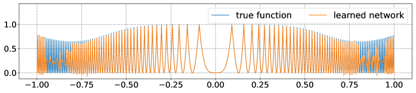
(a) $\mathtt{ReLU}$ MMNN of size $(434,16,6)$.

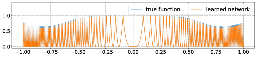
(b) $\mathtt{Sine}$ MMNN of size $(434,16,6)$.

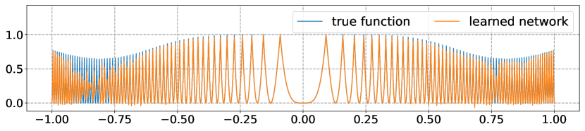
(c) $\mathtt{ReLU}$ MMNN of size $(900,16,6)$.

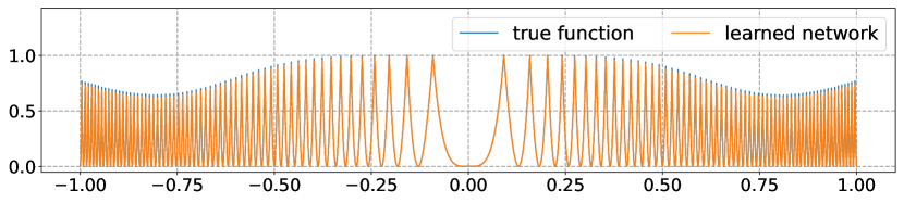
(d) $\mathtt{Sine}$ MMNN of size $(900,16,6)$.

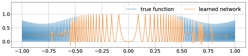
(e) $\mathtt{ReLU}$ FCNN of size $(120,-,6)$.

(f) $\mathtt{Sine}$ FCNN of size $(120,-,6)$.

Figure 7: Illustrations of the true function $f_{2}$ and learned networks.

For the test corresponding to $f_{2}$, we use a total of 60000 uniformly sampled points from $[-1,1]$ for training. The mini-batch size is set to 3000, and the learning rate is defined as $10^{-3}\times 0.9^{\lfloor k/500\rfloor}$, where $k=1,2,\mathinner{\mkern-0.1mu\cdotp\mkern-0.3mu\cdotp\mkern-0.3mu\cdotp\mkern-0.1mu},50000$ denotes the epoch number. To ensure accurate computation of the test error, we select another set of 60000 test samples from the uniform distribution $\mathcal{U}(-1,1)$. As illustrated in Figure 7, the MMNN architecture exhibits superior efficiency relative to the FCNN. Additionally, the $\mathtt{sine}$ activation function proves more effective than ReLU for approximating the complex target function $f_{2}$. It is worth noting that our training process involved a sufficiently large number of iterations, effectively eliminating the possibility of inadequate training as a contributing factor. Moreover, expanding the size of the MMNN would further substantially improve its performance. As shown in Table 2, MMNNs generally outperform FCNNs, regardless of the activation function. This advantage may stem from the simpler optimization landscape of MMNNs, which enables more efficient training. Furthermore, Table 2 highlights that $\mathtt{SinTU}$s achieve the best performance, which is expected since $f_{2}$ contains many singularities that $\mathtt{SinTU}$s are well-suited to handle. Notably, even in this inherently unfavorable setting for $\mathtt{sine}$-based models, $\mathtt{sine}$-activated MMNNs still perform well. Thus, when the properties of the target function are uncertain in practical applications, trying the $\mathtt{sine}$ activation function first is a reasonable strategy. When the mini-batch size is relatively large, the number of training epochs tends to be high, making the process time-consuming. More importantly, even when $\mathtt{sine}$-activated FCNNs are given sufficiently large mini-batches and a sufficient number of training epochs, their final performance still falls short of $\mathtt{sine}$-activated MMNNs.

For the test corresponding to $f_{3}$, we use a total of 18000 uniformly sampled points from $[-1,1]$ for training. The mini-batch size is set to $n_{\textnormal{mbs}}\in\{500,1000,1500,2000\}$, and the learning rate is defined as $10^{-3}\times 0.9^{\lfloor 2k/n_{\textnormal{mbs}}\rfloor}$, where $k=1,2,\mathinner{\mkern-0.1mu\cdotp\mkern-0.3mu\cdotp\mkern-0.3mu\cdotp\mkern-0.1mu},50n_{\textnormal{mbs}}$ denotes the epoch number. To ensure accurate computation of the test error, we select another set of 18000 test samples from the uniform distribution $\mathcal{U}(-1,1)$. As shown in Table 2, FCNNs are relatively sensitive to the hyper-parameters of training. If the mini-batch size is too small, training may fail. However, MMNNs are more stable and succeed under various settings.

3.2 MMNNs: Sine Versus Other Activation Functions

In this section, we compare the performance of MMNNs using different activation functions to demonstrate that FMMNNs consistently produce the best results. The three target functions used in the tests are $f_{1}:[-1,1]\to{\mathbb{R}}$, $f_{2}:[-1,1]^{2}\to{\mathbb{R}}$, and $f_{3}:[-1,1]^{3}\to{\mathbb{R}}$, which are given by

$$f_{1}(x)=0.6\sin(200\pi x)+0.8\cos(160\pi x^{2})+\frac{1+8x^{8}}{1+10x^{4}}\cdot\left|180x-2\left\lfloor\frac{180x+1}{2}\right\rfloor\right|,$$

$$f_{2}(x_{1},x_{2})=\sum_{i=1}^{2}\sum_{j=1}^{2}a_{ij}\sin(b_{i}x_{i}+c_{ij}x_{i}x_{j})\cdot\big{|}\cos(b_{j}x_{j}+d_{ij}x_{i}^{2})\big{|},$$

and

$$f_{3}(x_{1},x_{2},x_{3})=\sum_{i=1}^{3}\sum_{j=1}^{3}{\widetilde{a}}_{ij}\sin({\widetilde{b}}_{i}x_{i}+{\widetilde{c}}_{ij}x_{i}x_{j})\cdot\big{|}\cos({\widetilde{b}}_{j}x_{j}+{\widetilde{d}}_{ij}x_{i}^{2})\big{|},$$

where

$$(a_{ij})=\begin{bmatrix}0.3&0.2\\ 0.2&0.3\end{bmatrix},\ (b_{i})=\begin{bmatrix}12\pi\\ 8\pi\end{bmatrix},\ (c_{ij})=\begin{bmatrix}4\pi&18\pi\\ 16\pi&10\pi\end{bmatrix},\ (d_{ij})=\begin{bmatrix}14\pi&12\pi\\ 18\pi&10\pi\end{bmatrix},$$

$$({\widetilde{a}}_{ij})=\begin{bmatrix}0.3&0.1&0.4\\ 0.2&0.3&0.1\\ 0.2&0.1&0.3\end{bmatrix},\ ({\widetilde{b}}_{i})=\begin{bmatrix}\pi\\ 4\pi\\ 3\pi\end{bmatrix},\ ({\widetilde{c}}_{ij})=\begin{bmatrix}2\pi&\pi&3\pi\\ 2\pi&3\pi&2\pi\\ 3\pi&\pi&\pi\end{bmatrix},\ \textnormal{and}\ ({\widetilde{d}}_{ij})=\begin{bmatrix}2\pi&3\pi&\pi\\ \pi&3\pi&2\pi\\ \pi&2\pi&3\pi\end{bmatrix}.$$

Note that all three functions are only continuous but not differentiable. Illustrations of these three functions are shown in Figure 8.

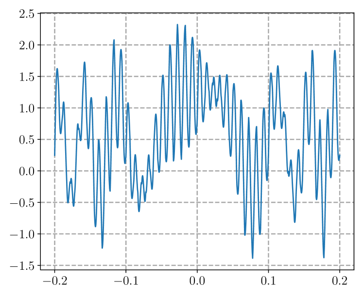
(a) $f_{1}$ limited on $[-0.2,0.2]$.

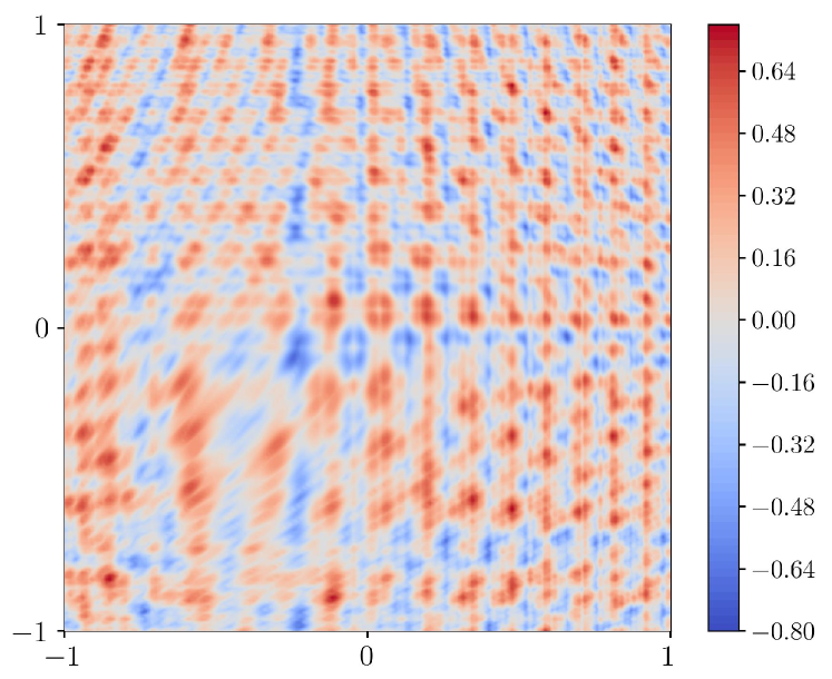
(b) $f_{2}$.

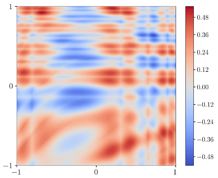
(c) $f_{3}(x,y,z=0)$.

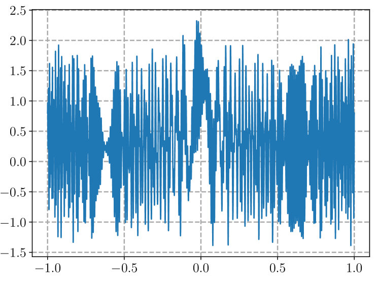
(d) $f_{1}$.

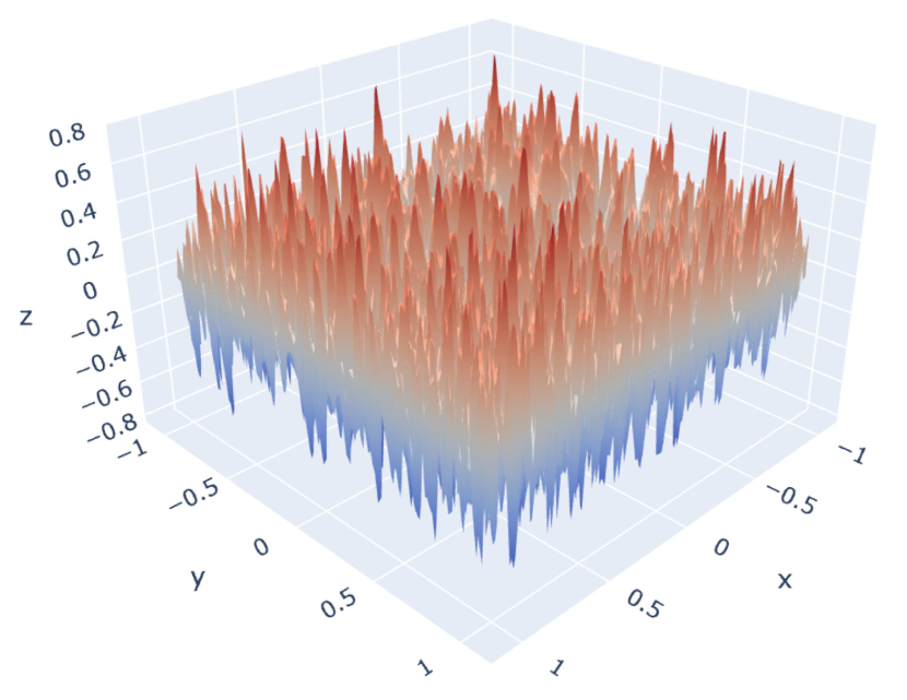
(e) $z=f_{2}(x,y)$.

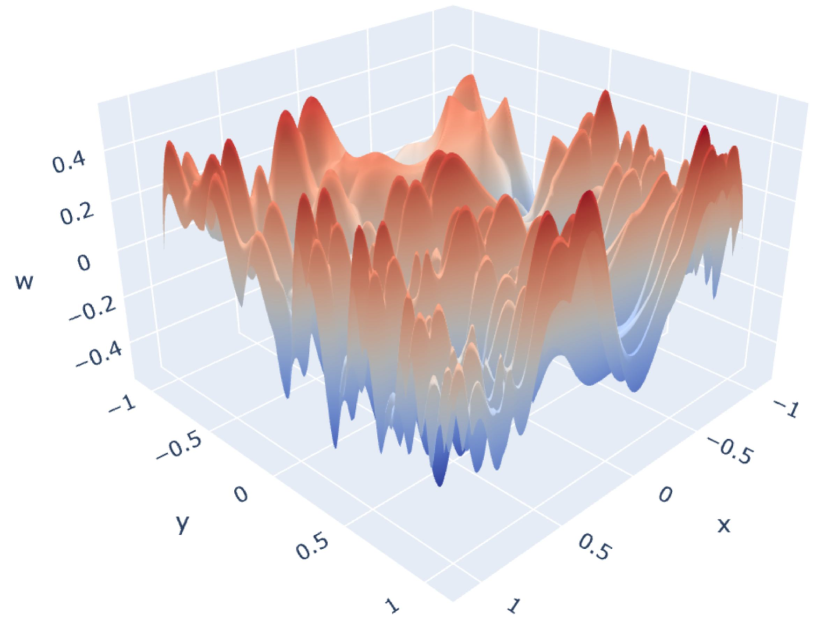
(f) $w=f_{3}(x,y,z=0)$.

Figure 8: Illustrations of $f_{i}$ for $i=1,2,3$.

We employ MMNN structures with different activation functions to approximate the target functions and evaluate their performance. For the one-dimensional case, we use 60000 uniformly sampled points from $[-1,1]$ for training, with a mini-batch size of 600 and a learning rate defined as $10^{-3}\times 0.9^{\lfloor k/100\rfloor}$, where $k=1,2,\mathinner{\mkern-0.1mu\cdotp\mkern-0.3mu\cdotp\mkern-0.3mu\cdotp\mkern-0.1mu},10000$ represents the epoch number. To ensure accurate computation of the test error, we select 60000 test samples from the uniform distribution in $[-1,1]$. In the two-dimensional case, $600^{2}$ uniformly sampled points from $[-1,1]^{2}$ are used for training, with a mini-batch size of 1200 and a learning rate set to $10^{-3}\times 0.9^{\lfloor k/30\rfloor}$, where $k=1,2,\mathinner{\mkern-0.1mu\cdotp\mkern-0.3mu\cdotp\mkern-0.3mu\cdotp\mkern-0.1mu},3000$. For test error evaluation, we select $300^{2}$ samples from the uniform distribution in $[-1,1]^{2}$. For the three-dimensional case, $150^{3}$ points from $[-1,1]^{3}$ are uniformly sampled for training, with a mini-batch size of 1500 and a learning rate defined as $10^{-3}\times 0.9^{\lfloor k/4\rfloor}$, where $k=1,2,\mathinner{\mkern-0.1mu\cdotp\mkern-0.3mu\cdotp\mkern-0.3mu\cdotp\mkern-0.1mu},400$. To ensure accurate computation of the test error, we select $100^{3}$ samples from the uniform distribution in $[-1,1]^{3}$.

Table 3: Comparison of test errors. Training is performed in single precision.

target function	$f_{1}:[-1,1]\to{\mathbb{R}}$		$f_{2}:[-1,1]^{2}\to{\mathbb{R}}$		$f_{3}:[-1,1]^{3}\to{\mathbb{R}}$
	MMNN of size (1024,16,6)		MMNN of size (1024,36,8)		ResMMNN of size (1024,36,10)
activation	MSE	MAX	MSE	MAX	MSE	MAX
$\mathtt{ReLU}$	$3.52\times 10^{-2}$	$1.57\times 10^{0}$	$6.50\times 10^{-5}$	$6.99\times 10^{-2}$	$8.18\times 10^{-5}$	$7.86\times 10^{-2}$
$\mathtt{ELU}$	$1.62\times 10^{-1}$	$1.78\times 10^{0}$	$2.43\times 10^{-3}$	$2.68\times 10^{-1}$	$6.70\times 10^{-5}$	$7.03\times 10^{-2}$
$\mathtt{GELU}$	$1.51\times 10^{-1}$	$1.61\times 10^{0}$	$6.19\times 10^{-5}$	$6.67\times 10^{-2}$	$6.66\times 10^{-5}$	$6.14\times 10^{-2}$
$\mathtt{sigmoid}$	$5.68\times 10^{-1}$	$1.95\times 10^{0}$	$4.97\times 10^{-2}$	$8.00\times 10^{-1}$	$1.04\times 10^{-3}$	$1.91\times 10^{-1}$
$\mathtt{tanh}$	$1.84\times 10^{-1}$	$1.77\times 10^{0}$	$9.76\times 10^{-4}$	$2.33\times 10^{-1}$	$1.06\times 10^{-4}$	$1.02\times 10^{-1}$
$\mathtt{sine}$	$1.16\times 10^{-5}$	$3.18\times 10^{-2}$	$2.26\times 10^{-5}$	$5.18\times 10^{-2}$	$\bm{2.67\times 10^{-5}}$	$5.22\times 10^{-2}$
$\mathtt{cosine}$	$1.55\times 10^{-5}$	$3.50\times 10^{-2}$	$2.46\times 10^{-5}$	$4.26\times 10^{-2}$	$3.06\times 10^{-5}$	$5.74\times 10^{-2}$
$\mathtt{SinTU}_{0}$	$2.14\times 10^{-6}$	$3.04\times 10^{-2}$	$3.18\times 10^{-5}$	$5.18\times 10^{-2}$	$4.21\times 10^{-5}$	$6.17\times 10^{-2}$
$\mathtt{SinTU}_{-\pi}$	$\bm{1.72\times 10^{-6}}$	$\bm{2.80\times 10^{-2}}$	$2.27\times 10^{-5}$	$5.38\times 10^{-2}$	$3.27\times 10^{-5}$	$5.56\times 10^{-2}$
$\mathtt{SinTU}_{-2\pi}$	$5.87\times 10^{-6}$	$3.17\times 10^{-2}$	$1.62\times 10^{-5}$	$\bm{3.90\times 10^{-2}}$	$2.85\times 10^{-5}$	$5.27\times 10^{-2}$
$\mathtt{SinTU}_{-4\pi}$	$1.21\times 10^{-5}$	$3.17\times 10^{-2}$	$\bm{1.52\times 10^{-5}}$	$4.73\times 10^{-2}$	$2.68\times 10^{-5}$	$5.43\times 10^{-2}$
$\mathtt{SinTU}_{-8\pi}$	$9.47\times 10^{-6}$	$3.03\times 10^{-2}$	$1.88\times 10^{-5}$	$4.53\times 10^{-2}$	$2.74\times 10^{-5}$	$\bm{5.16\times 10^{-2}}$

As shown in Table 3, sine and $\mathtt{SinTU}$s are the most effective activation functions for MMNNs. Our results further confirm that the combination of sinusoidal activations and MMNN structures is particularly well-suited for function approximation.

4 Proofs of Theorems 2.1 and 2.2

In this section, we establish the proofs of Theorems 2.1 and 2.2. To facilitate understanding, Section 4.1 provides a concise overview of the notations used throughout the paper. In Section 4.2, we outline the main ideas behind the proofs of Theorems 2.1 and 2.2. Additionally, for simplification, we introduce two propositions whose proofs are deferred to later sections. Assuming the validity of these propositions, we present the full detailed proofs of Theorems 2.1 and 2.2 in Section 4.

4.1 Notations

Below is a summary of the fundamental notations used throughout this paper.

• The difference between two sets $A$ and $B$ is denoted by $A\backslash B\coloneqq\{x:x\in A,\ x\notin B\}$.

• The symbols $\mathbb{N}$, $\mathbb{Z}$, $\mathbb{Q}$, and $\mathbb{R}$ represent the sets of natural numbers (including 0), integers, rational numbers, and real numbers, respectively. We denote the set of positive natural numbers by $\mathbb{N}^{+}=\mathbb{N}\backslash\{0\}=\{1,2,3,\mathinner{\mkern-0.1mu\cdotp\mkern-0.3mu\cdotp\mkern-0.3mu\cdotp\mkern-0.1mu}\}$.

• The floor and ceiling functions of a real number $x$ are given by $\lfloor x\rfloor=\max\{n:n\leq x,\ n\in\mathbb{Z}\}$ and $\lceil x\rceil=\min\{n:n\geq x,\ n\in\mathbb{Z}\}$.

• For any $p\in[1,\infty]$, the $p$-norm (or $\ell^{p}$-norm) of a vector $\bm{x}=(x_{1},\mathinner{\mkern-0.1mu\cdotp\mkern-0.3mu\cdotp\mkern-0.3mu\cdotp\mkern-0.1mu},x_{d})\in\mathbb{R}^{d}$ is defined as

  $$\|\bm{x}\|_{p}=\|\bm{x}\|_{\ell^{p}}\coloneqq\big{(}|x_{1}|^{p}+\mathinner{\mkern-0.1mu\cdotp\mkern-0.3mu\cdotp\mkern-0.3mu\cdotp\mkern-0.1mu}+|x_{d}|^{p}\big{)}^{1/p}\quad\text{for }p\in[1,\infty),$$

  and

  $$\|\bm{x}\|_{\infty}=\|\bm{x}\|_{\ell^{\infty}}\coloneqq\max\big{\{}|x_{i}|:i=1,2,\mathinner{\mkern-0.1mu\cdotp\mkern-0.3mu\cdotp\mkern-0.3mu\cdotp\mkern-0.1mu},d\big{\}}.$$

• Let $\textsf{{CPwL}}(n)$ denote the space of all continuous piecewise linear functions on ${\mathbb{R}}$ with at most $n\in{\mathbb{N}}$ breakpoints.

• The supremum norm of a bounded vector-valued function ${\bm{f}}:\Omega\subseteq{\mathbb{R}}^{d}\to{\mathbb{R}}^{n}$ is defined as

  $$\|{\bm{f}}\|_{\sup(\Omega)}\coloneqq\sup\big{\{}|f_{i}({\bm{x}})|:{\bm{x}}\in\Omega,\ i\in\{1,2,\mathinner{\mkern-0.1mu\cdotp\mkern-0.3mu\cdotp\mkern-0.3mu\cdotp\mkern-0.1mu},n\}\big{\}},$$

  where $f_{i}$ represents the $i$-th component of ${\bm{f}}$ for $i=1,2,\mathinner{\mkern-0.1mu\cdotp\mkern-0.3mu\cdotp\mkern-0.3mu\cdotp\mkern-0.1mu},n$.

• The symbol “$\rightrightarrows$” denotes uniform convergence. Specifically, if ${\bm{f}}:{\mathbb{R}}^{d}\to{\mathbb{R}}^{n}$ is a vector-valued function and ${\bm{f}}_{\delta}({\bm{x}})\rightrightarrows{\bm{f}}({\bm{x}})$ as $\delta\to 0$ for all ${\bm{x}}\in\Omega\subseteq{\mathbb{R}}^{d}$, then for any $\varepsilon>0$, there exists $\delta_{\varepsilon}\in(0,1)$ such that

  $$\|{\bm{f}}_{\delta}-{\bm{f}}\|_{\sup(\Omega)}<\varepsilon\quad\text{for all }\delta\in(0,\delta_{\varepsilon}).$$

• We adopt slicing notation for vectors and matrices. Given a vector ${\bm{x}}=(x_{1},\mathinner{\mkern-0.1mu\cdotp\mkern-0.3mu\cdotp\mkern-0.3mu\cdotp\mkern-0.1mu},x_{d})\in\mathbb{R}^{d}$, the notation ${\bm{x}}[n:m]$ refers to the slice from the $n$-th to the $m$-th entry for any $n,m\in\{1,2,\mathinner{\mkern-0.1mu\cdotp\mkern-0.3mu\cdotp\mkern-0.3mu\cdotp\mkern-0.1mu},d\}$ with $n\leq m$, while ${\bm{x}}[n]$ represents the $n$-th entry. For example, if ${\bm{x}}=(x_{1},x_{2},x_{3})\in\mathbb{R}^{3}$, then $(6{\bm{x}})[2:3]=(6x_{2},6x_{3})$ and $(8{\bm{x}}+1)[3]=8x_{3}+1.$ Similarly, for a matrix ${\bm{A}}$, the notation ${\bm{A}}[:,i]$ denotes its $i$-th column, while ${\bm{A}}[i,:]$ represents its $i$-th row. Moreover, ${\bm{A}}[i,n:m]$ is equivalent to $({\bm{A}}[i,:])[n:m]$, extracting the $n$-th to $m$-th entries from the $i$-th row.

4.2 Ideas and Propositions for Proving Theorems 2.1 and 2.2

Before presenting the detailed proofs of Theorems 2.1 and 2.2, let us first outline the key ideas underlying our approach. The main strategy in the proof involves constructing a piecewise constant function that approximates the desired continuous target function. However, achieving a uniform approximation with piecewise constants is challenging due to the continuity of ReLU and $\mathtt{sine}$ functions. To address this, we design networks that approximate piecewise constant behavior over most of the domain, specifically outside a small region, ensuring that the approximation error remains well-controlled. Within this small region, the error is manageable, as its measure can be made arbitrarily small.

With this foundation, we now proceed to the details. We divide the domain $[0,1]^{d}$ into a collection of “important” cubes, denoted $\{Q_{k}\}_{k\in\{1,2,\mathinner{\mkern-0.1mu\cdotp\mkern-0.3mu\cdotp\mkern-0.3mu\cdotp\mkern-0.1mu},M^{d}\}}$, along with a “negligible” region $\Omega$, where $M=N^{L}$. Each cube $Q_{k}$ is associated with a representative point $\bm{x}_{k}\in Q_{k}$. An illustration of $\bm{x}_{k}$, $\Omega$, and $Q_{k}$ can be seen in Figure 9. The construction of the desired network to approximate the target function is organized into two main steps below.

1. First, we construct a sub-network that realizes a function $\phi_{1}$ which maps each cube $Q_{k}$ to its respective index $k$. Specifically, we have $\phi_{1}(\bm{x})=k$ for any $\bm{x}\in Q_{k}$ and $k\in\{1,2,\mathinner{\mkern-0.1mu\cdotp\mkern-0.3mu\cdotp\mkern-0.3mu\cdotp\mkern-0.1mu},M^{d}\}$.

2. Next, we design a sub-network to implement a function $\phi_{2}$ that maps each index $k$ approximately to $f(\bm{x}_{k})$. Consequently, we obtain $\phi_{2}\circ\phi_{1}(\bm{x})=\phi_{2}(k)\approx f(\bm{x}_{k})\approx f(\bm{x})$ for any $\bm{x}\in Q_{k}$ and $k\in\{1,2,\mathinner{\mkern-0.1mu\cdotp\mkern-0.3mu\cdotp\mkern-0.3mu\cdotp\mkern-0.1mu},M^{d}\}$, implying that $\phi_{2}\circ\phi_{1}\approx f$ outside of $\Omega$.

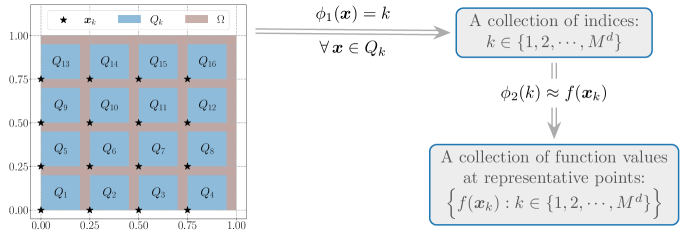
Figure 9: An illustration of the approach for constructing a network to approximate $f$. Observe that $\phi_{2}\circ\phi_{1}\approx f$ outside of $\Omega$, as $\phi_{2}\circ\phi_{1}(\bm{x})=\phi_{2}(k)\approx f(\bm{x}_{k})\approx f(\bm{x})$ for any $\bm{x}\in Q_{k}$ and $k\in\{1,2,\mathinner{\mkern-0.1mu\cdotp\mkern-0.3mu\cdotp\mkern-0.3mu\cdotp\mkern-0.1mu},M^{d}\}$.

The floor function is quite effective for handling the first step. To simplify the final proof, we introduce Proposition 4.1 below, which demonstrates how to construct a network that efficiently approximates the floor function. The proof of Proposition 4.1 is provided in Section 5.1.

Proposition 4.1.

Given any $\delta\in(0,1)$ and $N,L\in{\mathbb{N}}^{+}$, there exists

$$\phi\in{\hskip 0.6pt\mathcal{M}\hskip 0.0pt\mathcal{N}\hskip-0.8pt}_{{\mathtt{ReLU}}}\big{\{}4N-1,\hskip 2.2pt3,\hskip 2.2ptL;\hskip 3.0297pt{{\mathbb{R}}}\hskip-1.0298pt\to\hskip-0.98pt{{\mathbb{R}}}\big{\}}$$

such that

$$\phi(x)=\lfloor x\rfloor\quad\textnormal{for any $x\in\bigcup_{k=0}^{N^{L}-1}\big{[}k,\,k+1-\delta\big{]}.$}$$

The purpose of $\phi_{2}$ is to map each $k$ approximately to $f({\bm{x}}_{k})$ for $k\in\{1,2,\mathinner{\mkern-0.1mu\cdotp\mkern-0.3mu\cdotp\mkern-0.3mu\cdotp\mkern-0.1mu},M^{d}\}$. Notably, in constructing $\phi_{2}$, we only need to ensure correct values at a finite set of points $\{1,2,\mathinner{\mkern-0.1mu\cdotp\mkern-0.3mu\cdotp\mkern-0.3mu\cdotp\mkern-0.1mu},M^{d}\}$, rather than over an entire continuous domain. This key insight significantly simplifies the design of a network that realizes $\phi_{2}$. However, even with this simplification, the $\mathtt{ReLU}$ activation function is not particularly effective for this type of point-matching problem. In Proposition 4.2 below, we demonstrate that the $\mathtt{sine}$ function is exceptionally efficient for this task. The proof of Proposition 4.2 is provided in Section 5.2.

Proposition 4.2.

Given any $\varepsilon>0$ and $y_{k}\in{\mathbb{R}}$ for $k=1,2,\mathinner{\mkern-0.1mu\cdotp\mkern-0.3mu\cdotp\mkern-0.3mu\cdotp\mkern-0.1mu},K$, there exist $u,v,w\in{\mathbb{R}}$ such that

$$\big{|}u\cdot\sin\big{(}v\cdot\sin(kw)\big{)}-y_{k}\big{|}<\varepsilon\quad\textnormal{for $k=1,2,\mathinner{\mkern-0.1mu\cdotp\mkern-0.3mu\cdotp\mkern-0.3mu\cdotp\mkern-0.1mu},K$.}$$

We remark that Proposition 4.2 can also be understood through the concept of density. Specifically, for any $K\in\mathbb{N}^{+}$, the set

$$\Bigg{\{}\bigg{(}u\cdot\sin\big{(}v\cdot\sin(w)\big{)},\;u\cdot\sin\big{(}v\cdot\sin(2w)\big{)},\;\mathinner{\mkern-0.1mu\cdotp\mkern-0.3mu\cdotp\mkern-0.3mu\cdotp\mkern-0.1mu},\;u\cdot\sin\big{(}v\cdot\sin(Kw)\big{)}\bigg{)}:u,v,w\in\mathbb{R}\Bigg{\}}$$

is dense in $\mathbb{R}^{K}$. Additionally, we note that in Proposition 4.2, we can set $u=\max\{|y_{k}|:k=1,2,\mathinner{\mkern-0.1mu\cdotp\mkern-0.3mu\cdotp\mkern-0.3mu\cdotp\mkern-0.1mu},K\}$.

When analyzing the approximation power of MMNNs activated by $\mathtt{SinTU}$s, we need to leverage the singularity of $\mathtt{SinTU}$s for spatial partitioning. To simplify this process, we use ${\mathtt{ReLU}}$ for spatial partitioning and employ sub-MMNNs activated by $\mathtt{SinTU}$s to reproduce/approximate $\mathtt{ReLU}$. Proposition 4.3 below is specifically introduced to streamline the proof. The detailed proof of Proposition 4.3 can be found in Section 5.3.

Proposition 4.3.

Given any $B>0$, $k\in{\mathbb{N}}$, and $\varrho\in{\mathcal{S}}$, there exists $\phi_{\eta}\in{\hskip 0.6pt\mathcal{F}\hskip-0.828pt\mathcal{N}\hskip-0.725pt}_{\varrho}\{2,\hskip 1.987pt1;\hskip 3.0297pt{{\mathbb{R}}}\hskip-1.0298pt\to\hskip-0.98pt{{\mathbb{R}}}\}$ for each $\eta\in(0,1)$ such that

$$\phi_{\eta}(x)\rightrightarrows{\mathtt{ReLU}}(x)\quad\textnormal{as}\ \eta\to 0^{+}\quad\textnormal{for any $x\in[-B,B]$.}$$

The above proposition demonstrates that two active $\varrho$-activated neurons are sufficient to approximate ${\mathtt{ReLU}}$ arbitrarily well.

4.3 Detailed Proofs of Theorems 2.1 and 2.2 Based on Propositions

We are now prepared to present the detailed proofs of Theorems 2.1 and 2.2, assuming the validity of Propositions 4.1 and 4.2, which will be proven in Sections 5.1 and 5.2, respectively.

Let $M=N^{L}$ and $\delta\in(0,1)$ be a small number determined later. We first divide $[0,1]^{d}$ into a set of sub-cubes and a small region. To this end, we define ${\widetilde{\bm{x}}}_{\bm{\beta}}\coloneqq{\bm{\beta}}/M$ and

$${\widetilde{Q}}_{\bm{\beta}}\coloneqq\Big{\{}{\bm{x}}=(x_{1},\mathinner{\mkern-0.1mu\cdotp\mkern-0.3mu\cdotp\mkern-0.3mu\cdotp\mkern-0.1mu},x_{d})\in[0,1]^{d}:x_{i}\in[\tfrac{\beta_{i}}{M},\tfrac{\beta_{i}+1-\delta}{M}],\ i=1,\mathinner{\mkern-0.1mu\cdotp\mkern-0.3mu\cdotp\mkern-0.3mu\cdotp\mkern-0.1mu},d\Big{\}}$$

for each $d$-dimensional index ${\bm{\beta}}=(\beta_{1},\mathinner{\mkern-0.1mu\cdotp\mkern-0.3mu\cdotp\mkern-0.3mu\cdotp\mkern-0.1mu},\beta_{d})\in\{0,1,\mathinner{\mkern-0.1mu\cdotp\mkern-0.3mu\cdotp\mkern-0.3mu\cdotp\mkern-0.1mu},M-1\}^{d}$. Then the “negligible” region $\Omega$, given by

$$\Omega=[0,1]^{d}\big{\backslash}\big{(}\cup_{\bm{\beta}\in\{0,1,\mathinner{\mkern-0.1mu\cdotp\mkern-0.3mu\cdotp\mkern-0.3mu\cdotp\mkern-0.1mu},M-1\}^{d}}{\widetilde{Q}}_{\bm{\beta}}\big{)},$$

has a sufficiently small measure for small $\delta$.

To simplify notation, we reindex the $d$-dimensional indices as one-dimensional indices. For this purpose, we establish a one-to-one mapping between $\{0,1,\mathinner{\mkern-0.1mu\cdotp\mkern-0.3mu\cdotp\mkern-0.3mu\cdotp\mkern-0.1mu},M-1\}^{d}$ and $\{1,2,\mathinner{\mkern-0.1mu\cdotp\mkern-0.3mu\cdotp\mkern-0.3mu\cdotp\mkern-0.1mu},M^{d}\}$, defined by

$$g(\bm{\beta})=1+\sum_{i=1}^{d}\beta_{i}\cdot M^{i-1}\quad\textnormal{for any ${\bm{\beta}}=(\beta_{1},\mathinner{\mkern-0.1mu\cdotp\mkern-0.3mu\cdotp\mkern-0.3mu\cdotp\mkern-0.1mu},\beta_{d})\in\{0,1,\mathinner{\mkern-0.1mu\cdotp\mkern-0.3mu\cdotp\mkern-0.3mu\cdotp\mkern-0.1mu},M-1\}^{d}$}.$$

Thus, for each $k\in\{1,2,\mathinner{\mkern-0.1mu\cdotp\mkern-0.3mu\cdotp\mkern-0.3mu\cdotp\mkern-0.1mu},M^{d}\}$, there exists a unique $\bm{\beta}\in\{0,1,\mathinner{\mkern-0.1mu\cdotp\mkern-0.3mu\cdotp\mkern-0.3mu\cdotp\mkern-0.1mu},M-1\}^{d}$ such that $g(\bm{\beta})=k$. Accordingly, we reindex $\widetilde{\bm{x}}_{\bm{\beta}}$ and $\widetilde{Q}_{\bm{\beta}}$ as $\bm{x}_{k}$ and $Q_{k}$, respectively. That is,

$$\bm{x}_{k}=\widetilde{\bm{x}}_{\bm{\beta}}\quad\textnormal{and}\quad Q_{k}=\widetilde{Q}_{\bm{\beta}}\quad\textnormal{with $k=g({\bm{\beta}})$}\quad\textnormal{for any ${\bm{\beta}}=(\beta_{1},\mathinner{\mkern-0.1mu\cdotp\mkern-0.3mu\cdotp\mkern-0.3mu\cdotp\mkern-0.1mu},\beta_{d})\in\{0,1,\mathinner{\mkern-0.1mu\cdotp\mkern-0.3mu\cdotp\mkern-0.3mu\cdotp\mkern-0.1mu},M-1\}^{d}$}.$$

See Figure 10 for illustrations of $\Omega$, ${\widetilde{Q}}_{\bm{\beta}}$, ${\widetilde{\bm{x}}}_{\bm{\beta}}$, $Q_{k}$, and ${\bm{x}}_{k}$ for ${\bm{\beta}}\in\{0,1,\mathinner{\mkern-0.1mu\cdotp\mkern-0.3mu\cdotp\mkern-0.3mu\cdotp\mkern-0.1mu},M-1\}^{d}$ and $k\in\{1,2,\mathinner{\mkern-0.1mu\cdotp\mkern-0.3mu\cdotp\mkern-0.3mu\cdotp\mkern-0.1mu},M^{d}\}$ when $M=4$ and $d=2$.

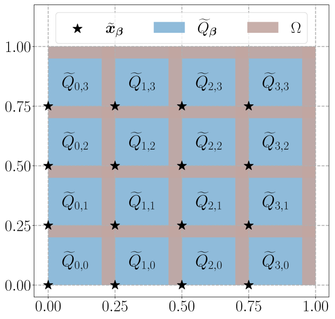
Figure 10: Illustrations of $\Omega$, ${\widetilde{Q}}_{\bm{\beta}}$, ${\widetilde{\bm{x}}}_{\bm{\beta}}$, $Q_{k}$, and ${\bm{x}}_{k}$ for ${\bm{\beta}}\in\{0,1,\mathinner{\mkern-0.1mu\cdotp\mkern-0.3mu\cdotp\mkern-0.3mu\cdotp\mkern-0.1mu},M-1\}^{d}$ and $k\in\{1,2,\mathinner{\mkern-0.1mu\cdotp\mkern-0.3mu\cdotp\mkern-0.3mu\cdotp\mkern-0.1mu},M^{d}\}$ when $M=4$ and $d=2$.

Next, we construct a network-realized function that maps $\bm{x}\in Q_{k}$ to $k$ for any $k\in\{1,2,\mathinner{\mkern-0.1mu\cdotp\mkern-0.3mu\cdotp\mkern-0.3mu\cdotp\mkern-0.1mu},M^{d}\}$. Fixing $\bm{x}=(x_{1},\mathinner{\mkern-0.1mu\cdotp\mkern-0.3mu\cdotp\mkern-0.3mu\cdotp\mkern-0.1mu},x_{d})\in Q_{k}$ for some $k\in\{1,2,\mathinner{\mkern-0.1mu\cdotp\mkern-0.3mu\cdotp\mkern-0.3mu\cdotp\mkern-0.1mu},M^{d}\}$, there exists a unique $\bm{\beta}=(\beta_{1},\mathinner{\mkern-0.1mu\cdotp\mkern-0.3mu\cdotp\mkern-0.3mu\cdotp\mkern-0.1mu},\beta_{d})$ such that $g(\bm{\beta})=k$. Then, $\bm{x}\in Q_{k}=\widetilde{Q}_{\bm{\beta}}$ implies

$$x_{i}\in\Big{[}\frac{\beta_{i}}{M},\;\frac{\beta_{i}+1-\delta}{M}\Big{]}\quad\textnormal{for }i=1,\mathinner{\mkern-0.1mu\cdotp\mkern-0.3mu\cdotp\mkern-0.3mu\cdotp\mkern-0.1mu},d,$$

from which we deduce

$$Mx_{i}\in[\beta_{i},\;\beta_{i}+1-\delta]\quad\textnormal{with }\beta_{i}\in\{0,1,\mathinner{\mkern-0.1mu\cdotp\mkern-0.3mu\cdotp\mkern-0.3mu\cdotp\mkern-0.1mu},M-1\}\quad\textnormal{ for }i=1,\mathinner{\mkern-0.1mu\cdotp\mkern-0.3mu\cdotp\mkern-0.3mu\cdotp\mkern-0.1mu},d.$$ (8)

By Proposition 4.1, there exists a function ${\psi}\in{\hskip 0.6pt\mathcal{F}\hskip-0.828pt\mathcal{N}\hskip-0.725pt}_{{\mathtt{ReLU}}}\big{\{}4N-1,\hskip 1.987ptL;\hskip 3.0297pt{\mathbb{R}}\hskip-1.0298pt\to\hskip-0.98pt{\mathbb{R}}\big{\}}$ such that

$${\psi}(x)=\lfloor x\rfloor\quad\text{for any }x\in\bigcup_{m=0}^{N^{L}-1}\big{[}m,m+1-\delta\big{]}=\bigcup_{m=0}^{M-1}\big{[}m,m+1-\delta\big{]}.$$

Then, by Equation (8), we have

$${\psi}(x_{i})=\beta_{i}\quad\text{for }i=1,\mathinner{\mkern-0.1mu\cdotp\mkern-0.3mu\cdotp\mkern-0.3mu\cdotp\mkern-0.1mu},d.$$

By defining

$${\bm{\Psi}}({\bm{y}})\coloneqq\Big{(}\psi(y_{1}),\psi(y_{2}),\mathinner{\mkern-0.1mu\cdotp\mkern-0.3mu\cdotp\mkern-0.3mu\cdotp\mkern-0.1mu},\psi(y_{d})\Big{)}\quad\textnormal{for any }{\bm{x}}=(y_{1},\mathinner{\mkern-0.1mu\cdotp\mkern-0.3mu\cdotp\mkern-0.3mu\cdotp\mkern-0.1mu},y_{d})\in{\mathbb{R}}^{d},$$

we have ${\bm{\Psi}}({\bm{x}})={\bm{\beta}}$, implying

$$g\circ{\bm{\Psi}}({\bm{x}})=g({\bm{\beta}})=k.$$

Since $\bm{x}\in Q_{k}$ and $k\in\{1,2,\mathinner{\mkern-0.1mu\cdotp\mkern-0.3mu\cdotp\mkern-0.3mu\cdotp\mkern-0.1mu},M^{d}\}$ are arbitrary, we have

$$g\circ{\bm{\Psi}}(\bm{x})=k\quad\textnormal{for any }\bm{x}\in Q_{k}\text{ and }k\in\{1,2,\mathinner{\mkern-0.1mu\cdotp\mkern-0.3mu\cdotp\mkern-0.3mu\cdotp\mkern-0.1mu},M^{d}\}.$$ (9)

To construct a function that maps $k\in\{1,2,\mathinner{\mkern-0.1mu\cdotp\mkern-0.3mu\cdotp\mkern-0.3mu\cdotp\mkern-0.1mu},M^{d}\}$ approximately to $f(\bm{x}_{k})$, we apply Proposition 4.2 with $K=M^{d}$ and $y_{k}=f(\bm{x}_{k})$. This yields the existence of constants $u,v,w\in\mathbb{R}$ such that

$$\left|u\cdot\sin\big{(}v\cdot\sin(kw)\big{)}-f({\bm{x}}_{k})\right|<\varepsilon\quad\text{for }k=1,2,\mathinner{\mkern-0.1mu\cdotp\mkern-0.3mu\cdotp\mkern-0.3mu\cdotp\mkern-0.1mu},M^{d},$$ (10)

where $\varepsilon>0$ is a small number to be determined later.

We define

$$\phi_{1}({\bm{y}})\coloneqq g\circ{\bm{\Psi}}({\bm{y}})\quad\textnormal{for any ${\bm{y}}\in{\mathbb{R}}^{d}$}$$

and

$$\phi_{2}(z)=u\cdot\sin\big{(}v\cdot\sin(wz)\big{)}\quad\textnormal{for any $z\in{\mathbb{R}}$.}$$

It is clear that $\psi\in{\hskip 0.6pt\mathcal{M}\hskip 0.0pt\mathcal{N}\hskip-0.8pt}_{{\mathtt{ReLU}}}\big{\{}4N-1,\hskip 2.2pt3,\hskip 2.2ptL;\hskip 3.0297pt{\mathbb{R}}\hskip-1.0298pt\to\hskip-0.98pt{\mathbb{R}}\big{\}}$ implies

$${\bm{\Psi}}\in{\hskip 0.6pt\mathcal{M}\hskip 0.0pt\mathcal{N}\hskip-0.8pt}_{{\mathtt{ReLU}}}\big{\{}d(4N-1),\hskip 2.2pt3d,\hskip 2.2ptL;\hskip 3.0297pt{\mathbb{R}^{d}}\hskip-1.0298pt\to\hskip-0.98pt{\mathbb{R}^{d}}\big{\}}.$$

Recall that $g:{\mathbb{R}}^{d}\to{\mathbb{R}}$ is an affine linear map. By combining $g$ with the final affine linear map (correspoding to $\bm{\Psi}$) into a new mapping, we obtain

$$\phi_{1}=g\circ{\bm{\Psi}}\in{\hskip 0.6pt\mathcal{M}\hskip 0.0pt\mathcal{N}\hskip-0.8pt}_{{\mathtt{ReLU}}}\big{\{}d(4N-1),\hskip 2.2pt3d,\hskip 2.2ptL;\hskip 3.0297pt{\mathbb{R}^{d}}\hskip-1.0298pt\to\hskip-0.98pt{\mathbb{R}^{d}}\big{\}}.$$

Since $\phi_{2}(z)=u\cdot\sin\big{(}v\cdot\sin(wz)\big{)}$, we have

$$\phi_{2}\circ\phi_{1}\in{\hskip 0.6pt\mathcal{M}\hskip 0.0pt\mathcal{N}\hskip-0.8pt}_{(\sin,{\mathtt{ReLU}})}\big{\{}d(4N-1),\hskip 2.2pt3d,\hskip 2.2ptL+2;\hskip 3.0297pt{\mathbb{R}}\hskip-1.0298pt\to\hskip-0.98pt{\mathbb{R}^{d}}\big{\}}.$$

To complete the proof of Theorem 2.2, where the corresponding $\phi$ is defined as $\phi\coloneqq\phi_{2}\circ\phi_{1}$, it remains to bound the approximation error. For any $\bm{x}\in Q_{k}$ and $k\in\{1,2,\mathinner{\mkern-0.1mu\cdotp\mkern-0.3mu\cdotp\mkern-0.3mu\cdotp\mkern-0.1mu},M^{d}\}$, by Equations (9) and (10), we have

$$\begin{split}|\phi_{2}\circ\phi_{1}({\bm{x}})-f({\bm{x}}_{k})|=\Big{|}\phi_{2}\Big{(}\underbrace{g\circ{\bm{\Psi}}({\bm{x}})}_{\textnormal{$=k$ by \eqref{eq:g:tildePsi:x:to:k}}}\Big{)}-f({\bm{x}}_{k})\Big{|}&=|\phi_{2}(k)-f({\bm{x}}_{k})|\\ &=\left|u\cdot\sin\big{(}v\cdot\sin(kw)\big{)}-f({\bm{x}}_{k})\right|<\varepsilon\end{split}$$

and $\|{\bm{x}}_{k}-{\bm{x}}\|_{2}\leq\tfrac{\sqrt{d(1-\delta)}}{M}\leq\frac{\sqrt{d}}{M}$, from which we deduce

$$\begin{split}|\phi_{2}\circ\phi_{1}({\bm{x}})-f({\bm{x}})|\leq|\phi_{2}\circ\phi_{1}({\bm{x}})-f({\bm{x}}_{k})|+|f({\bm{x}}_{k})-f({\bm{x}})|\leq\varepsilon+\omega_{f}(\tfrac{\sqrt{d}}{M}).\end{split}$$

Recall that

$$\bigcup_{k\in\{0,1,\mathinner{\mkern-0.1mu\cdotp\mkern-0.3mu\cdotp\mkern-0.3mu\cdotp\mkern-0.1mu},M^{d}-1\}}Q_{k}=[0,1]^{d}\setminus\Omega\quad\textnormal{ and}\quad\|\phi_{2}\circ\phi_{1}\|_{L^{\infty}([0,1]^{d})}\leq\|\phi_{2}\|_{L^{\infty}(\mathbb{R})}\leq|u|,$$

where $u$ is a constant determined by $f$ and is independent of $\delta$. Therefore

$$\begin{split}\|\phi_{2}\circ\phi_{1}-f\|_{L^{p}([0,1]^{d})}^{p}&=\int_{\Omega}|\phi_{2}\circ\phi_{1}({\bm{x}})-f({\bm{x}})|^{p}\textnormal{d}{\bm{x}}+\int_{[0,1]^{d}\backslash\Omega}|\phi_{2}\circ\phi_{1}({\bm{x}})-f({\bm{x}})|^{p}\textnormal{d}{\bm{x}}\\ &\leq\mu(\Omega)\cdot\|\phi_{2}\circ\phi_{1}-f\|_{L^{\infty}(\Omega)}^{p}+\sum_{k=1}^{M^{d}}\int_{Q_{k}}|\phi_{2}\circ\phi_{1}({\bm{x}})-f({\bm{x}})|^{p}\textnormal{d}{\bm{x}}\\ &\leq\mu(\Omega)\cdot\Big{(}|u|+\|f\|_{L^{\infty}([0,1]^{d})}\Big{)}^{p}+\sum_{k=1}^{M^{d}}\mu(Q_{k})\cdot\Big{(}\varepsilon+\omega_{f}(\tfrac{\sqrt{d}}{M})\Big{)}^{p}\\ &\leq\mu(\Omega)\cdot\Big{(}|u|+\|f\|_{L^{\infty}([0,1]^{d})}\Big{)}^{p}+\Big{(}\varepsilon+\omega_{f}(\tfrac{\sqrt{d}}{M})\Big{)}^{p}\leq\Big{(}\tfrac{11}{10}\omega_{f}(\tfrac{\sqrt{d}}{M})\Big{)}^{p}\end{split}$$

where the last inequality is achieved by setting

$$\varepsilon=\tfrac{1}{11}\omega_{f}(\tfrac{\sqrt{d}}{M})>0$$

and choosing a sufficiently small $\delta\in(0,1)$ to make $\mu(\Omega)$ small enough, ensuring that

$$\mu(\Omega)\cdot\Big{(}|u|+\|f\|_{L^{\infty}([0,1]^{d})}\Big{)}^{p}\leq\Big{(}\tfrac{11}{10}\omega_{f}(\tfrac{\sqrt{d}}{M})\Big{)}^{p}-\Big{(}\tfrac{12}{11}\omega_{f}(\tfrac{\sqrt{d}}{M})\Big{)}^{p}>0.$$

We note that the condition $\omega_{f}\big{(}\frac{\sqrt{d}}{M}\big{)}>0$ can be satisfied; otherwise, $f$ would be a constant function, which is a trivial case. That is, we obtain

$$\begin{split}\|\phi_{2}\circ\phi_{1}-f\|_{L^{p}([0,1]^{d})}\leq\tfrac{11}{10}\omega_{f}(\tfrac{\sqrt{d}}{M}).\end{split}$$ (11)

Recall that $\omega_{f}(n\cdot t)\leq n\cdot\omega_{f}(t)$ for any $n\in{\mathbb{N}}^{+}$ and $t\in[0,\infty)$. Thus, we have

$$\begin{split}\|\phi-f\|_{L^{p}([0,1]^{d})}\leq\tfrac{11}{10}\omega_{f}(\tfrac{\sqrt{d}}{M})\leq\tfrac{11}{10}\omega_{f}(\tfrac{\lceil\sqrt{d}\rceil}{M})\leq\tfrac{11}{10}\big{\lceil}\sqrt{d}\big{\rceil}\cdot\omega_{f}(\tfrac{1}{M})\leq 2\sqrt{d}\cdot\omega_{f}(N^{-L}),\end{split}$$

where the last inequality follows from $M=N^{L}$ and the fact that $\frac{11}{10}\lceil\sqrt{n}\,\rceil\leq 2\sqrt{n}$ for any $n\in\mathbb{N}^{+}$. This completes the proof of Theorem 2.2.

Recall that $\varrho\in\mathcal{S}$ is a $\mathtt{SinTU}$ activation function. To complete the proof of Theorem 2.1, it is necessary to implement/approximate $\phi_{1}$ and $\phi_{2}$ using $\varrho$-activated MMNNs, rather than $\mathtt{ReLU}$ or ${\mathtt{sine}}$ as was done in the proof of Theorem 2.2.

First, we will construct $\phi_{1,\eta}\in{\hskip 0.6pt\mathcal{M}\hskip 0.0pt\mathcal{N}\hskip-0.8pt}_{\varrho}\{2d(4N-1),\hskip 2.2pt3d,\hskip 2.2ptL;\hskip 3.0297pt{{\mathbb{R}}^{d}}\hskip-1.0298pt\to\hskip-0.98pt{{\mathbb{R}}}\}$ for any $\eta\in(0,1)$ such that

$$\phi_{1,\eta}({\bm{x}})\rightrightarrows\phi_{1}({\bm{x}})\quad\textnormal{as}\ \eta\to 0^{+}\quad\textnormal{for any ${\bm{x}}\in[0,1]^{d}$.}$$

To this end, we first construct a $\varrho$-activation MMNN to approximate the $\mathtt{ReLU}$ function, since $\phi_{1}\in{\hskip 0.6pt\mathcal{M}\hskip 0.0pt\mathcal{N}\hskip-0.8pt}_{{\mathtt{ReLU}}}\{2d(4N-1),\hskip 2.2pt3d,\hskip 2.2ptL;\hskip 3.0297pt{{\mathbb{R}}^{d}}\hskip-1.0298pt\to\hskip-0.98pt{{\mathbb{R}}}\}$. Without loss of generality, we assume that $\phi_{1}$ can be expressed as a composition of functions

$$\phi_{1}({\bm{x}})={\mathcal{A}}_{L}\circ{\mathtt{ReLU}}\circ{\mathcal{\widehat{A}}}_{L-1}\circ{\mathcal{\widetilde{A}}}_{L-1}\circ\ \mathinner{\mkern-0.1mu\cdotp\mkern-0.3mu\cdotp\mkern-0.3mu\cdotp\mkern-0.1mu}\ \circ{\mathtt{ReLU}}\circ{\mathcal{\widehat{A}}}_{1}\circ{\mathcal{\widetilde{A}}}_{1}\circ{\mathtt{ReLU}}\circ{\mathcal{A}}_{0}({\bm{x}})\quad\textnormal{for any ${\bm{x}}\in{\mathbb{R}}^{d}$},$$

where ${\mathcal{A}}_{0}:{\mathbb{R}}^{d}\to{\mathbb{R}}^{3d(4N-1)}$, ${\bm{\mathcal{\widetilde{A}}}}_{\ell}:{\mathbb{R}}^{3d(4N-1)}\to{\mathbb{R}}^{3d}$, ${\bm{\mathcal{\widehat{A}}}}_{\ell}:{\mathbb{R}}^{3d}\to{\mathbb{R}}^{3d(4N-1)}$, and ${\mathcal{A}}_{L}:{\mathbb{R}}^{3d(4N-1)}\to{\mathbb{R}}$ are affine linear maps for any $\ell\in\{1,2,\mathinner{\mkern-0.1mu\cdotp\mkern-0.3mu\cdotp\mkern-0.3mu\cdotp\mkern-0.1mu},L-1\}$. By setting ${\mathcal{A}}_{\ell}={\bm{\mathcal{\widehat{A}}}}_{\ell}\circ{\bm{\mathcal{\widetilde{A}}}}_{\ell}$ for any $\ell\in\{1,2,\mathinner{\mkern-0.1mu\cdotp\mkern-0.3mu\cdotp\mkern-0.3mu\cdotp\mkern-0.1mu},L-1\}$, we have

$$\phi_{1}({\bm{x}})={\mathcal{A}}_{L}\circ{\mathtt{ReLU}}\circ{\mathcal{A}}_{L-1}\circ\ \mathinner{\mkern-0.1mu\cdotp\mkern-0.3mu\cdotp\mkern-0.3mu\cdotp\mkern-0.1mu}\ \circ{\mathtt{ReLU}}\circ{\mathcal{A}}_{1}\circ{\mathtt{ReLU}}\circ{\mathcal{A}}_{0}({\bm{x}})\quad\textnormal{for any ${\bm{x}}\in{\mathbb{R}}^{d}$},$$

Since $\varrho\in{\mathcal{S}}$, by Proposition 4.3, there exists $\sigma_{\eta}\in{\hskip 0.6pt\mathcal{F}\hskip-0.828pt\mathcal{N}\hskip-0.725pt}_{\varrho}\{2,\hskip 1.987pt1;\hskip 3.0297pt{{\mathbb{R}}}\hskip-1.0298pt\to\hskip-0.98pt{{\mathbb{R}}}\}$ for each $\eta\in(0,1)$ such that

$$\sigma_{\eta}(x)\rightrightarrows{\mathtt{ReLU}}(x)\quad\textnormal{as}\ \eta\to 0^{+}\quad\textnormal{for any $x\in[-B,B]$,}$$

where $B>0$ is a large number determined later.

For each $\eta\in(0,1)$, we define

$$\phi_{1,\eta}({\bm{x}})={\mathcal{A}}_{L}\circ\sigma_{\eta}\circ{\mathcal{A}}_{L-1}\circ\ \mathinner{\mkern-0.1mu\cdotp\mkern-0.3mu\cdotp\mkern-0.3mu\cdotp\mkern-0.1mu}\ \circ\sigma_{\eta}\circ{\mathcal{A}}_{1}\circ\sigma_{\eta}\circ{\mathcal{A}}_{0}({\bm{x}})\quad\textnormal{for any ${\bm{x}}\in{\mathbb{R}}^{d}$}.$$

In other words,

$$\phi_{1,\eta}({\bm{x}})={\mathcal{A}}_{L}\circ\sigma_{\eta}\circ{\mathcal{\widehat{A}}}_{L-1}\circ{\mathcal{\widetilde{A}}}_{L-1}\circ\ \mathinner{\mkern-0.1mu\cdotp\mkern-0.3mu\cdotp\mkern-0.3mu\cdotp\mkern-0.1mu}\ \circ\sigma_{\eta}\circ{\mathcal{\widehat{A}}}_{1}\circ{\mathcal{\widetilde{A}}}_{1}\circ\sigma_{\eta}\circ{\mathcal{A}}_{0}({\bm{x}})\quad\textnormal{for any ${\bm{x}}\in{\mathbb{R}}^{d}$}.$$

Recall that $\sigma_{\eta}\in{\hskip 0.6pt\mathcal{F}\hskip-0.828pt\mathcal{N}\hskip-0.725pt}_{\varrho}\{2,\hskip 1.987pt1;\hskip 3.0297pt{{\mathbb{R}}}\hskip-1.0298pt\to\hskip-0.98pt{{\mathbb{R}}}\}$. To replace the ReLU activation function with $\sigma_{\eta}$ in a network, we substitute each ReLU with two $\varrho$-activated neurons. Consequently, $\phi_{1}\in{\hskip 0.6pt\mathcal{M}\hskip 0.0pt\mathcal{N}\hskip-0.8pt}_{\varrho}\{d(4N-1),\hskip 2.2pt3d,\hskip 2.2ptL;\hskip 3.0297pt{{\mathbb{R}}^{d}}\hskip-1.0298pt\to\hskip-0.98pt{{\mathbb{R}}}\}$ implies

$$\phi_{1,\eta}\in{\hskip 0.6pt\mathcal{M}\hskip 0.0pt\mathcal{N}\hskip-0.8pt}_{\varrho}\{2d(4N-1),\hskip 2.2pt3d,\hskip 2.2ptL;\hskip 3.0297pt{{\mathbb{R}}^{d}}\hskip-1.0298pt\to\hskip-0.98pt{{\mathbb{R}}}\}.$$

Next, we will prove

$$\phi_{1,\eta}({\bm{x}})\rightrightarrows\phi_{1}({\bm{x}})\quad\textnormal{as}\ \eta\to 0^{+}\quad\textnormal{for any ${\bm{x}}\in[0,1]^{d}$}.$$

For each $\eta\in(0,1)$ and $\ell=0,1,\mathinner{\mkern-0.1mu\cdotp\mkern-0.3mu\cdotp\mkern-0.3mu\cdotp\mkern-0.1mu},L$, let ${\bm{h}}_{\ell}$ and ${\bm{h}}_{\ell,\eta}$ denote the functions represented by the first $\ell$ hidden layers of the MMNNs corresponding to $\phi_{1}$ and $\phi_{1,\eta}$, respectively, i.e.,

$${\bm{h}}_{\ell}({\bm{x}})\coloneqq{\mathcal{A}}_{\ell}\circ{\mathtt{ReLU}}\circ{\mathcal{A}}_{\ell-1}\circ\ \mathinner{\mkern-0.1mu\cdotp\mkern-0.3mu\cdotp\mkern-0.3mu\cdotp\mkern-0.1mu}\ \circ{\mathtt{ReLU}}\circ{\mathcal{A}}_{1}\circ{\mathtt{ReLU}}\circ{\mathcal{A}}_{0}({\bm{x}})\quad\textnormal{for any ${\bm{x}}\in{\mathbb{R}}^{d}$}$$

and

$${\bm{h}}_{\ell,\eta}({\bm{x}})\coloneqq{\mathcal{A}}_{\ell}\circ\sigma_{\eta}\circ{\mathcal{A}}_{\ell-1}\circ\ \mathinner{\mkern-0.1mu\cdotp\mkern-0.3mu\cdotp\mkern-0.3mu\cdotp\mkern-0.1mu}\ \circ\sigma_{\eta}\circ{\mathcal{A}}_{1}\circ\sigma_{\eta}\circ{\mathcal{A}}_{0}({\bm{x}})\quad\textnormal{for any ${\bm{x}}\in{\mathbb{R}}^{d}$}.$$

For $\ell=0,1,\mathinner{\mkern-0.1mu\cdotp\mkern-0.3mu\cdotp\mkern-0.3mu\cdotp\mkern-0.1mu},L$, we will prove by induction that

$${\bm{h}}_{\ell,\eta}({\bm{x}})\rightrightarrows{\bm{h}}_{\ell}({\bm{x}})\quad\textnormal{as}\ \eta\to 0^{+}\quad\textnormal{for any ${\bm{x}}\in[0,1]^{d}$.}$$ (12)

First, we consider the base case $\ell=0$. Clearly,

$${\bm{h}}_{0,\eta}({\bm{x}})={\mathcal{A}}_{0}({\bm{x}})={\bm{h}}_{0}({\bm{x}})\rightrightarrows{\bm{h}}_{0}({\bm{x}})\quad\textnormal{as}\ \eta\to 0^{+}\quad\textnormal{for any ${\bm{x}}\in[0,1]^{d}$.}$$

This means Equation (12) holds for $\ell=0$.

Next, supposing Equation (12) holds for $\ell=i\in\{0,1,\mathinner{\mkern-0.1mu\cdotp\mkern-0.3mu\cdotp\mkern-0.3mu\cdotp\mkern-0.1mu},L-1\}$, our goal is to prove that it also holds for $\ell=i+1$. Determine $B>0$ via

$$B=\max\Big{\{}\|{\bm{h}}_{j}\|_{\sup([0,1]^{d})}+1:j=0,1,\mathinner{\mkern-0.1mu\cdotp\mkern-0.3mu\cdotp\mkern-0.3mu\cdotp\mkern-0.1mu},L\Big{\}},$$

where the continuity of ${\mathtt{ReLU}}$ guarantees the above supremum is finite, i.e., $M\in[1,\infty)$. By the induction hypothesis, we have

$${\bm{h}}_{i,\eta}({\bm{x}})\rightrightarrows{\bm{h}}_{i}({\bm{x}})\quad\textnormal{as}\ \eta\to 0^{+}\quad\textnormal{for any ${\bm{x}}\in[0,1]^{d}$.}$$

Clearly, for any ${\bm{x}}\in[0,1]^{d}$, we have $\|{\bm{h}}_{i}({\bm{x}})\|_{\ell^{\infty}}\leq B$ and

$$\|{\bm{h}}_{i,\eta}({\bm{x}})\|_{\ell^{\infty}}\leq\|{\bm{h}}_{i}({\bm{x}})\|_{\ell^{\infty}}+1\leq B\quad\textnormal{ for small $\eta>0$.}$$

Recall that $\sigma_{\eta}(t)\rightrightarrows{\mathtt{ReLU}}(t)$ as $\eta\to 0^{+}$ for any $t\in[-B,B]$. Then, we have

$$\sigma_{\eta}\circ{\bm{h}}_{i,\eta}({\bm{x}})-{\mathtt{ReLU}}\circ{\bm{h}}_{i,\eta}({\bm{x}})\rightrightarrows{\bm{0}}\quad\textnormal{as}\ \eta\to 0^{+}\quad\textnormal{for any ${\bm{x}}\in[0,1]^{d}$.}$$

The continuity of ${\mathtt{ReLU}}$ implies the uniform continuity of ${\mathtt{ReLU}}$ on $[-B,B]$, from which we deduce

$${\mathtt{ReLU}}\circ{\bm{h}}_{i,\eta}({\bm{x}})-{\mathtt{ReLU}}\circ{\bm{h}}_{i}({\bm{x}})\rightrightarrows{\bm{0}}\quad\textnormal{as}\ \eta\to 0^{+}\quad\textnormal{for any ${\bm{x}}\in[0,1]^{d}$.}$$

Therefore, for any ${\bm{x}}\in[0,1]^{d}$, as $\eta\to 0^{+}$, we have

$$\sigma_{\eta}\circ{\bm{h}}_{i,\eta}({\bm{x}})-{\mathtt{ReLU}}\circ{\bm{h}}_{i}({\bm{x}})=\underbrace{\sigma_{\eta}\circ{\bm{h}}_{i,\eta}({\bm{x}})-{\mathtt{ReLU}}\circ{\bm{h}}_{i,\eta}({\bm{x}})}_{\rightrightarrows{\bm{0}}}+\underbrace{{\mathtt{ReLU}}\circ{\bm{h}}_{i,\eta}({\bm{x}})-{\mathtt{ReLU}}\circ{\bm{h}}_{i}({\bm{x}})}_{\rightrightarrows{\bm{0}}}\rightrightarrows{\bm{0}},$$

from which we deduce

$${\bm{h}}_{i+1,\eta}({\bm{x}})={\mathcal{A}}_{i+1}\circ\sigma_{\eta}\circ{\bm{h}}_{i,\eta}({\bm{x}})\rightrightarrows{\mathcal{A}}_{i+1}\circ{\mathtt{ReLU}}\circ{\bm{h}}_{i}({\bm{x}})={\bm{h}}_{i+1}({\bm{x}}).$$

This means Equation (12) holds for $\ell=i+1$. So we complete the inductive step.

By the principle of induction, we have

$$\phi_{1,{\eta}}({\bm{x}})={\bm{h}}_{L,\eta}({\bm{x}})\rightrightarrows{\bm{h}}_{L}({\bm{x}})=\phi_{1}({\bm{x}})\quad\textnormal{as}\ \eta\to 0^{+}\quad\textnormal{for any ${\bm{x}}\in[0,1]^{d}$}.$$

Next, we consider replacing ${\mathtt{sine}}$ in $\phi_{2}$ with $\varrho$. Since $\varrho\in{\mathcal{S}}$, there exists $s\in{\mathbb{R}}$ such that $\varrho(x)=\sin(x)$ for all $x\geq s$. Since $\phi_{1}$ is bounded on $[0,1]^{d}$, there exists a sufficiently large integer $m\in\mathbb{Z}$ such that

$$2m\pi+w\cdot\phi_{1}({\bm{x}})\geq s\quad\text{and}\quad 2m\pi+v\cdot\sin\big{(}w\cdot\phi_{1}({\bm{x}})\big{)}\geq s\quad\textnormal{for any ${\bm{x}}\in[0,1]^{d}$},$$

from which we deduce

$$\begin{split}&\phantom{=\;\;}\sin\Big{(}v\cdot\sin\big{(}w\cdot\phi_{1}({\bm{x}})\big{)}\Big{)}=\sin\Big{(}\underbrace{2m\pi+v\cdot\sin\big{(}w\cdot\phi_{1}({\bm{x}})\big{)}}_{\geq\;s}\Big{)}=\varrho\Big{(}2m\pi+v\cdot\sin\big{(}w\cdot\phi_{1}({\bm{x}})\big{)}\Big{)}\\ &=\varrho\Big{(}2m\pi+v\cdot\sin\big{(}\underbrace{2m\pi+w\cdot\phi_{1}({\bm{x}})}_{\geq\;s}\big{)}\Big{)}=\varrho\Big{(}2m\pi+v\cdot\varrho\big{(}2m\pi+w\cdot\phi_{1}({\bm{x}})\big{)}\Big{)}.\end{split}$$

Then by defining

$${\widetilde{\phi}}_{2}(y)\coloneqq u\cdot\varrho\Big{(}2m\pi+v\cdot\varrho\big{(}2m\pi+wy\big{)}\Big{)}\quad\textnormal{for any $y\in{\mathbb{R}}$,}$$

for any ${\bm{x}}\in[0,1]^{d}$, we have

$$\begin{split}{\widetilde{\phi}}_{2}\circ\phi_{1}({\bm{x}})&=u\cdot\varrho\Big{(}2m\pi+v\cdot\varrho\big{(}2m\pi+w\cdot\phi_{1}({\bm{x}})\big{)}\Big{)}\\ &=u\cdot\sin\Big{(}v\cdot\sin\big{(}w\cdot\phi_{1}({\bm{x}})\big{)}\Big{)}=\phi_{2}\cdot\phi_{1}({\bm{x}}).\end{split}$$ (13)

Recall that

$$|\phi_{1,{\eta}}({\bm{x}})|\leq|\phi_{1}({\bm{x}})|+1\leq B\quad\textnormal{ for small $\eta>0$ and any ${\bm{x}}\in[0,1]^{d}$}.$$

The continuity of ${\widetilde{\phi}}_{2}$ implies the uniform continuity of ${\widetilde{\phi}}_{2}$ on $[-B,B]$, from which we deduce

$${\widetilde{\phi}}_{2}\circ\phi_{1,{\eta}}({\bm{x}})\rightrightarrows{\widetilde{\phi}}_{2}\circ\phi_{1}({\bm{x}})\quad\textnormal{as}\ \eta\to 0\quad\textnormal{for any ${\bm{x}}\in[0,1]^{d}$}.$$

Then we can choose sufficiently small $\eta_{0}>0^{+}$ such that

$$\|{\widetilde{\phi}}_{2}\circ\phi_{1,{\eta_{0}}}-{\widetilde{\phi}}_{2}\circ\phi_{1}\|_{L^{p}([0,1]^{d})}\leq\tfrac{1}{10}\omega_{f}(\tfrac{\sqrt{d}}{M}).$$ (14)

Now we can define the desired $\phi$ for Theorem 2.1 via $\phi\coloneqq{\widetilde{\phi}}_{2}\circ\phi_{1,{\eta_{0}}}$.

By Equations (11), (13), and (14), we have

$$\begin{split}\|{\widetilde{\phi}}_{2}\circ\phi_{1,{\eta_{0}}}-f\|_{L^{p}([0,1]^{d})}&\leq\|{\widetilde{\phi}}_{2}\circ\phi_{1,{\eta_{0}}}-{\widetilde{\phi}}_{2}\circ\phi_{1}\|_{L^{p}([0,1]^{d})}+\|{\widetilde{\phi}}_{2}\circ\phi_{1}-f\|_{L^{p}([0,1]^{d})}\\ &\leq\tfrac{1}{10}\omega_{f}(\tfrac{\sqrt{d}}{M})+\|\phi_{2}\circ\phi_{1}-f\|_{L^{p}([0,1]^{d})}\\ &\leq\tfrac{1}{10}\omega_{f}(\tfrac{\sqrt{d}}{M})+\tfrac{11}{10}\omega_{f}(\tfrac{\sqrt{d}}{M})=\tfrac{6}{5}\omega_{f}(\tfrac{\sqrt{d}}{M}).\end{split}$$

Recall that $\omega_{f}(n\cdot t)\leq n\cdot\omega_{f}(t)$ for any $n\in{\mathbb{N}}^{+}$ and $t\in[0,\infty)$. Thus, we have

$$\begin{split}\|{\widetilde{\phi}}_{2}\circ\phi_{1,{\eta_{0}}}-f\|_{L^{p}([0,1]^{d})}\leq\tfrac{6}{5}\omega_{f}(\tfrac{\sqrt{d}}{M})\leq\tfrac{6}{5}\omega_{f}(\tfrac{\lceil\sqrt{d}\rceil}{M})\leq\tfrac{6}{5}\big{\lceil}\sqrt{d}\big{\rceil}\cdot\omega_{f}(\tfrac{1}{M})\leq 2\sqrt{d}\cdot\omega_{f}(N^{-L}),\end{split}$$

where the last inequality follows from $M=N^{L}$ and the fact that $\frac{6}{5}\lceil\sqrt{n}\,\rceil\leq 2\sqrt{n}$ for any $n\in\mathbb{N}^{+}$. Recall that ${\widetilde{\phi}}_{2}(y)\coloneqq u\cdot\varrho\Big{(}2m\pi+v\cdot\varrho\big{(}2m\pi+wy\big{)}\Big{)}$ for any $y\in{\mathbb{R}}$ and

$$\phi_{1,\eta_{0}}\in{\hskip 0.6pt\mathcal{M}\hskip 0.0pt\mathcal{N}\hskip-0.8pt}_{\varrho}\{2d(4N-1),\hskip 2.2pt3d,\hskip 2.2ptL;\hskip 3.0297pt{{\mathbb{R}}^{d}}\hskip-1.0298pt\to\hskip-0.98pt{{\mathbb{R}}}\}.$$

We conclude that

$${\widetilde{\phi}}_{2}\circ\phi_{1,\eta_{0}}\in{\hskip 0.6pt\mathcal{M}\hskip 0.0pt\mathcal{N}\hskip-0.8pt}_{\varrho}\{2d(4N-1),\hskip 2.2pt3d,\hskip 2.2ptL+2;\hskip 3.0297pt{{\mathbb{R}}^{d}}\hskip-1.0298pt\to\hskip-0.98pt{{\mathbb{R}}}\},$$

which completes the proof of Theorem 2.1.

5 Proofs of Propositions in Section 4.2

In this section, we present the detailed proofs of all propositions stated in Section 4.2. Specifically, the proofs of Propositions 4.1, 4.2, and 4.3 are provided in Sections 5.1, 5.2, and 5.3, respectively.

5.1 Proof of Proposition 4.1

We will prove Proposition 4.1, which demonstrates the efficiency of $\mathtt{ReLU}$ FCNNs in approximating the floor function. The core idea is to use compositions of continuous piecewise functions to approximate the floor function effectively. To simplify the proof, we introduce a lemma below, which shows that continuous piecewise functions can be exactly represented by one-hidden-layer $\mathtt{ReLU}$ FCNNs.

Lemma 5.1.

For any $n\in{\mathbb{N}}^{+}$, it holds that

$$\textsf{{CPwL}}\big{(}n\big{)}\subseteq{\hskip 0.6pt\mathcal{F}\hskip-0.828pt\mathcal{N}\hskip-0.725pt}_{{\mathtt{ReLU}}}\big{\{}n+1,\hskip 1.987pt1;\hskip 3.0297pt{{\mathbb{R}}}\hskip-1.0298pt\to\hskip-0.98pt{{\mathbb{R}}}\big{\}}.$$ (15)

Proof.

We proceed by mathematical induction to prove Equation (15). We begin with the base case $n=1$. For any $f\in\textsf{{CPwL}}\big{(}1\big{)}$, there exist $a_{1},a_{2},x_{0}\in\mathbb{R}$ such that

$$f(x)=\begin{cases}a_{1}(x-x_{0})+f(x_{0})&\text{if }x\geq x_{0},\\ a_{2}(x_{0}-x)+f(x_{0})&\text{if }x<x_{0}.\end{cases}$$

Thus, we can express $f(x)$ as $f(x)=a_{1}\sigma(x-x_{0})+a_{2}\sigma(x_{0}-x)+f(x_{0})$ for any $x\in\mathbb{R}$, which implies $f\in{\hskip 0.6pt\mathcal{F}\hskip-0.828pt\mathcal{N}\hskip-0.725pt}_{{\mathtt{ReLU}}}\big{\{}2,\hskip 1.987pt1;\hskip 3.0297pt{\mathbb{R}}\hskip-1.0298pt\to\hskip-0.98pt{\mathbb{R}}\big{\}}.$ Therefore, Equation (15) holds for $n=1$.

Now, suppose Equation (15) holds for $n=k\in\mathbb{N}^{+}$. We aim to show that it also holds for $n=k+1$. For any $f\in\textsf{{CPwL}}\big{(}k+1\big{)}$, we assume without loss of generality that $f$ has a largest breakpoint at $x_{0}$ (the case where $f$ has no breakpoints is trivial). Let $a_{1}$ and $a_{2}$ represent the slopes of the linear segments directly to the left and right of $x_{0}$, respectively. Define

$$\widetilde{f}(x)\coloneqq f(x)-(a_{2}-a_{1})\sigma(x-x_{0})\quad\text{for any }x\in\mathbb{R}.$$

With this construction, $\widetilde{f}$ has slope $a_{1}$ on both sides of $x_{0}$, effectively smoothing out the breakpoint at $x_{0}$ in $f$. Thus, $\widetilde{f}$ is obtained by eliminating this breakpoint, leaving it with at most $k$ breakpoints. By the induction hypothesis, we know that

$$\widetilde{f}\in\textsf{{CPwL}}\big{(}k\big{)}\subseteq{\hskip 0.6pt\mathcal{F}\hskip-0.828pt\mathcal{N}\hskip-0.725pt}_{{\mathtt{ReLU}}}\big{\{}k+1,\hskip 1.987pt1;\hskip 3.0297pt{\mathbb{R}}\hskip-1.0298pt\to\hskip-0.98pt{\mathbb{R}}\big{\}}.$$

Thus, there exist constants $u_{j},v_{j},w_{j},c$ for $j=1,2,\mathinner{\mkern-0.1mu\cdotp\mkern-0.3mu\cdotp\mkern-0.3mu\cdotp\mkern-0.1mu},k+1$ such that

$$\widetilde{f}(x)=\sum_{j=1}^{k+1}u_{j}\sigma(v_{j}x+w_{j})+c\quad\text{for any }x\in\mathbb{R}.$$

Therefore, for any $x\in\mathbb{R}$, we can write

$$f(x)=(a_{2}-a_{1})\sigma(x-x_{0})+\widetilde{f}(x)=(a_{2}-a_{1})\sigma(x-x_{0})+\sum_{j=1}^{k+1}u_{j}\sigma(v_{j}x+w_{j})+c,$$

implying that $f\in{\hskip 0.6pt\mathcal{F}\hskip-0.828pt\mathcal{N}\hskip-0.725pt}_{{\mathtt{ReLU}}}\big{\{}k+2,\hskip 1.987pt1;\hskip 3.0297pt{\mathbb{R}}\hskip-1.0298pt\to\hskip-0.98pt{\mathbb{R}}\big{\}}$. Thus, Equation (15) holds for $k+1$, completing the induction process and, hence, the proof of Lemma 5.1. ∎

With Lemma 5.1 established, we are now ready to prove Proposition 4.1.

Proof of Proposition 4.1.

Given any $x\in\bigcup_{k=0}^{N^{L}-1}\big{[}k,\,k+1-\delta\big{]}$, our goal is to construct $\phi$, realized by a network with desired size, mapping $x$ to $\lfloor x\rfloor$. Clearly $\lfloor x\rfloor\in\{0,1,\mathinner{\mkern-0.1mu\cdotp\mkern-0.3mu\cdotp\mkern-0.3mu\cdotp\mkern-0.1mu},N^{L}-1\}$ and hence there exists unique $(n_{1},n_{2},\mathinner{\mkern-0.1mu\cdotp\mkern-0.3mu\cdotp\mkern-0.3mu\cdotp\mkern-0.1mu},n_{L})\in\{0,1,\mathinner{\mkern-0.1mu\cdotp\mkern-0.3mu\cdotp\mkern-0.3mu\cdotp\mkern-0.1mu},N-1\}^{L}$ such that

$$\lfloor x\rfloor=\sum_{i=1}^{L}n_{i}\cdot N^{L-i}.$$ (16)

In other words, the above equation forms a one-to-one map between $\{0,1,\mathinner{\mkern-0.1mu\cdotp\mkern-0.3mu\cdotp\mkern-0.3mu\cdotp\mkern-0.1mu},N^{L}-1\}$ and $\{0,1,\mathinner{\mkern-0.1mu\cdotp\mkern-0.3mu\cdotp\mkern-0.3mu\cdotp\mkern-0.1mu},N-1\}^{L}$.

For $\ell=0,1,\mathinner{\mkern-0.1mu\cdotp\mkern-0.3mu\cdotp\mkern-0.3mu\cdotp\mkern-0.1mu},L$, we define

$$m_{\ell}=\sum_{i=\ell+1}^{L}n_{i}\cdot N^{L-i}\quad\textnormal{and}\quad z_{\ell}=x-\sum_{i=1}^{\ell}n_{i}\cdot N^{L-i}.$$

Clearly, $z_{0}=x$,

$$\begin{split}z_{\ell}=x-\lfloor x\rfloor+\lfloor x\rfloor-\sum_{i=\ell+1}^{L}n_{i}\cdot N^{L-i}&=x-\lfloor x\rfloor+\sum_{i=1}^{L}n_{i}\cdot N^{L-i}-\sum_{i=\ell+1}^{L}n_{i}\cdot N^{L-i}\\ &=x-\lfloor x\rfloor+\sum_{i=1}^{\ell}n_{i}\cdot N^{L-i}=x-\lfloor x\rfloor+m_{\ell},\end{split}$$

and

$$\begin{split}\lfloor z_{\ell}\rfloor=\Big{\lfloor}\underbrace{x-\lfloor x\rfloor}_{\in\,[0,1)}+\underbrace{m_{\ell}}_{\in\,{\mathbb{Z}}}\Big{\rfloor}&=m_{\ell}\end{split}$$

for $\ell=0,1,\mathinner{\mkern-0.1mu\cdotp\mkern-0.3mu\cdotp\mkern-0.3mu\cdotp\mkern-0.1mu},L$. We claim

$$n_{\ell+1}\leq\frac{z_{\ell}}{N^{L-\ell-1}}\leq n_{\ell+1}+1-\frac{\delta}{N^{L-\ell-1}}\quad\textnormal{for $\ell=0,1,\mathinner{\mkern-0.1mu\cdotp\mkern-0.3mu\cdotp\mkern-0.3mu\cdotp\mkern-0.1mu},L-1$}.$$ (17)

To demonstrate this, we first establish the lower bound. Clearly,

$$\frac{z_{\ell}}{N^{L-\ell}}=\frac{x-\lfloor x\rfloor+m_{\ell}}{N^{L-\ell-1}}\geq\frac{m_{\ell}}{N^{L-\ell-1}}=\frac{\sum_{i=\ell+1}^{L}n_{i}\cdot N^{L-i}}{N^{L-\ell-1}}\geq\frac{n_{\ell+1}\cdot N^{L-(\ell+1)}}{N^{L-\ell-1}}=n_{\ell+1}.$$

Next, we proceed to verify the upper bound. Clearly,

$$\begin{split}\frac{z_{\ell}}{N^{L-\ell-1}}=\frac{x-\lfloor x\rfloor+m_{\ell}}{N^{L-\ell-1}}&=\frac{x-\lfloor x\rfloor+\delta+m_{\ell}}{N^{L-\ell-1}}-\frac{\delta}{N^{L-\ell-1}}\\ &\leq\frac{1+m_{\ell}}{N^{L-\ell-1}}-\frac{\delta}{N^{L-\ell-1}}\leq n_{\ell}+1-\frac{\delta}{N^{L-\ell}},\end{split}$$

where the last inequality come from

$$\begin{split}\frac{1+m_{\ell}}{N^{L-\ell-1}}=\frac{1+\sum_{i=\ell+1}^{L}n_{i}\cdot N^{L-i}}{N^{L-\ell-1}}&=\frac{1+\sum_{i=\ell+2}^{L}n_{i}\cdot N^{L-i}+n_{\ell+1}\cdot N^{L-(\ell+1)}}{N^{L-\ell-1}}\\ &\leq\frac{1+\sum_{i=\ell+2}^{L}(N-1)\cdot N^{L-i}+n_{\ell+1}\cdot N^{L-(\ell+1)}}{N^{L-\ell-1}}\\ &=\frac{N^{L-\ell-1}+n_{\ell+1}\cdot N^{L-(\ell+1)}}{N^{L-\ell-1}}=n_{\ell}+1.\end{split}$$

Thus, we complete the proof of Equation (17).

Let $h$ be a continuous piecewise linear function with $h\in\textsf{{CPwL}}(2N-2)$ and

$$h(k)=h\Big{(}k+1-\frac{\delta}{N^{L-1}}\Big{)}=k\quad\textnormal{for $k=0,1,\mathinner{\mkern-0.1mu\cdotp\mkern-0.3mu\cdotp\mkern-0.3mu\cdotp\mkern-0.1mu},N-1$}.$$

Figure 11: An illustration of $h$ when $N=5$.

See Figure 11 for an illustration of $h$ when $N=5$. Obviously,

$$h(t)=k\quad\textnormal{if $t\in\Big{[}k,\;k+1-\frac{\delta}{N^{L-1}}\Big{]}$}\quad\textnormal{for $k=0,1,\mathinner{\mkern-0.1mu\cdotp\mkern-0.3mu\cdotp\mkern-0.3mu\cdotp\mkern-0.1mu},N-1$.}$$

For $\ell=0,1,\mathinner{\mkern-0.1mu\cdotp\mkern-0.3mu\cdotp\mkern-0.3mu\cdotp\mkern-0.1mu},L-1$, we have $n_{\ell+1}\in\{0,1,\mathinner{\mkern-0.1mu\cdotp\mkern-0.3mu\cdotp\mkern-0.3mu\cdotp\mkern-0.1mu},N-1\}$ and Equation (17) implies

$$\frac{z_{\ell}}{N^{L-\ell-1}}\in\Big{[}n_{\ell+1},\;n_{\ell+1}+1-\frac{\delta}{N^{L-\ell-1}}\Big{]}\subseteq\Big{[}n_{\ell+1},\;n_{\ell+1}+1-\frac{\delta}{N^{L-1}}\Big{]}.$$

It follows that

$$h\Big{(}\frac{z_{\ell}}{N^{L-\ell-1}}\Big{)}=n_{\ell+1}\quad\textnormal{for $\ell=0,1,\mathinner{\mkern-0.1mu\cdotp\mkern-0.3mu\cdotp\mkern-0.3mu\cdotp\mkern-0.1mu},L-1$,}$$

from which we deduce

$$\begin{split}z_{\ell+1}=x-\sum_{i=1}^{\ell+1}n_{i}\cdot N^{L-i}&=x-\sum_{i=1}^{\ell}n_{i}\cdot N^{L-i}-n_{\ell+1}\cdot N^{L-(\ell+1)}\\ &=z_{\ell}-n_{\ell+1}\cdot N^{L-(\ell+1)}=z_{\ell}-h\Big{(}\frac{z_{\ell}}{N^{L-\ell-1}}\Big{)}\cdot N^{L-\ell-1}.\end{split}$$

Therefore, by defining

$$h_{\ell}(z)=h\Big{(}\frac{z}{N^{L-\ell-1}}\Big{)}\quad\textnormal{and}\quad{\widetilde{h}}_{\ell}(z)=z-h\Big{(}\frac{z}{N^{L-\ell-1}}\Big{)}\cdot N^{L-\ell-1}\quad\textnormal{for any $z\in{\mathbb{R}}$,}$$

we have

$$h_{\ell}(z_{\ell})=n_{\ell+1}\quad\textnormal{and}\quad{\widetilde{h}}_{\ell}(z_{\ell})=z_{\ell+1}\quad\textnormal{for $\ell=0,1,\mathinner{\mkern-0.1mu\cdotp\mkern-0.3mu\cdotp\mkern-0.3mu\cdotp\mkern-0.1mu},L-1$.}$$ (18)

Moreover, $h\in\textsf{{CPwL}}(2N-2)$ implies $h_{\ell},{\widetilde{h}}_{\ell}\in\textsf{{CPwL}}(2N-2)$ for $\ell=0,1,\mathinner{\mkern-0.1mu\cdotp\mkern-0.3mu\cdotp\mkern-0.3mu\cdotp\mkern-0.1mu},L-1$. Then by Lemma 5.1,

$$h_{\ell},{\widetilde{h}}_{\ell}\in\textsf{{CPwL}}(2N-2)\subseteq{\hskip 0.6pt\mathcal{F}\hskip-0.828pt\mathcal{N}\hskip-0.725pt}_{{\mathtt{ReLU}}}\big{\{}2N-1,\hskip 1.987pt1;\hskip 3.0297pt{{\mathbb{R}}}\hskip-1.0298pt\to\hskip-0.98pt{{\mathbb{R}}}\big{\}}.$$ (19)

This means that $h_{\ell}$ and $\widetilde{h}_{\ell}$ can be implemented by one-hidden-layer $\mathtt{ReLU}$ FCNNs of width $2N-1$.

Consequently, the desired function $\phi$ can be realized by a $\mathtt{ReLU}$ MMNN of width $1+(2N-1)+(2N-1)=4N-1$, rank $3$, and depth $L$, as illustrated in Figure 12. That is,

$$\phi\in{\hskip 0.6pt\mathcal{M}\hskip 0.0pt\mathcal{N}\hskip-0.8pt}_{{\mathtt{ReLU}}}\big{\{}4N-1,\hskip 2.2pt3,\hskip 2.2ptL;\hskip 3.0297pt{{\mathbb{R}}}\hskip-1.0298pt\to\hskip-0.98pt{{\mathbb{R}}}\big{\}},$$

which completes the proof of Proposition 4.1. ∎

Figure 12: The target network implementing $\phi$ based on Equations (16), (18), and (19). In this architecture, redundant (fake) layers can be removed by merging the preceding and succeeding affine linear transformations into a single one.

5.2 Proof of Proposition 4.2

We will establish the proof of Proposition 4.2. To facilitate this, we introduce two key lemmas that serve as intermediate steps in proving Proposition 4.2. The first lemma demonstrates how to use the $\mathtt{sine}$ function with a single parameter to generate rationally independent numbers. The second lemma shows the density of point sets generated by the $\mathtt{sine}$ function combined with rational numbers within a high-dimensional hypercube.

Lemma 5.2.

Given $K\in{\mathbb{N}}^{+}$, there exists $w_{0}\in\big{(}-\tfrac{1}{K},\tfrac{1}{K}\big{)}$ such that $\sin(kw_{0})$, for $k=1,2,\mathinner{\mkern-0.1mu\cdotp\mkern-0.3mu\cdotp\mkern-0.3mu\cdotp\mkern-0.1mu},K$, are rationally independent.

Lemma 5.3.

Given any rationally independent numbers $a_{1},a_{2},\mathinner{\mkern-0.1mu\cdotp\mkern-0.3mu\cdotp\mkern-0.3mu\cdotp\mkern-0.1mu},a_{K}$, for any $K\in{\mathbb{N}}^{+}$, the following set

$$\Big{\{}\Big{(}\sin(wa_{1}),\,\sin(wa_{2}),\,\mathinner{\mkern-0.1mu\cdotp\mkern-0.3mu\cdotp\mkern-0.3mu\cdotp\mkern-0.1mu},\,\sin(wa_{K})\Big{)}:w\in{\mathbb{R}}\Big{\}}$$

is dense in $[-1,1]^{K}$.

We are now prepared to prove Proposition 4.2, assuming the validity of Lemmas 5.2 and 5.1, which will be proven in Sections 5.2.1 and 5.2.2, respectively.

Proof of Proposition 4.2.

Given any $\varepsilon>0$ and $y_{k}\in\mathbb{R}$ for $k=1,2,\mathinner{\mkern-0.1mu\cdotp\mkern-0.3mu\cdotp\mkern-0.3mu\cdotp\mkern-0.1mu},K$, we define

$$u\coloneqq\max\big{\{}|y_{k}|:k=1,2,\mathinner{\mkern-0.1mu\cdotp\mkern-0.3mu\cdotp\mkern-0.3mu\cdotp\mkern-0.1mu},K\big{\}}.$$

Assuming $u>0$ (the case $u=0$ is trivial), we set $z_{k}=y_{k}/u\leq 1$. Then, by Lemma 5.2, there exists $w$ such that $a_{k}=\sin(kw)$ for $k=1,2,\mathinner{\mkern-0.1mu\cdotp\mkern-0.3mu\cdotp\mkern-0.3mu\cdotp\mkern-0.1mu},K$ are rationally independent. Moreover, by Lemma 5.3, the following set

$$\Big{\{}\big{[}\sin(va_{1}),\,\sin(va_{2}),\,\mathinner{\mkern-0.1mu\cdotp\mkern-0.3mu\cdotp\mkern-0.3mu\cdotp\mkern-0.1mu},\,\sin(va_{K})\big{]}^{\textsf{{T}}}:v\in{\mathbb{R}}\Big{\}}$$

is dense in $[-1,1]^{K}$. That is, there exists $v\in{\mathbb{R}}$ such that

$$\big{|}\sin(va_{k})-z_{k}\big{|}\leq\varepsilon/u\quad\textnormal{for $k=1,2,\mathinner{\mkern-0.1mu\cdotp\mkern-0.3mu\cdotp\mkern-0.3mu\cdotp\mkern-0.1mu},K$.}$$

Therefore, for $k=1,2,\mathinner{\mkern-0.1mu\cdotp\mkern-0.3mu\cdotp\mkern-0.3mu\cdotp\mkern-0.1mu},K$, we have

$$\begin{split}\Big{|}u\cdot\sin\big{(}v\cdot\sin(kw)\big{)}-y_{k}\Big{|}&=u\Big{|}\sin\big{(}v\cdot\sin(kw)\big{)}-y_{k}/u\Big{|}\\ &=u\big{|}\sin\big{(}v\cdot a_{k}\big{)}-z_{k}\big{|}<u\cdot\varepsilon/u=\varepsilon.\end{split}$$

So we finish the proof of Proposition 4.2. ∎

5.2.1 Proof of Lemma 5.2

We prove this lemma by contradiction. If it does not hold, then $\sin(kw)$, for $k=1,2,\mathinner{\mkern-0.1mu\cdotp\mkern-0.3mu\cdotp\mkern-0.3mu\cdotp\mkern-0.1mu},K$, are rationally dependent for any $w\in\big{(}-\tfrac{1}{K},\tfrac{1}{K}\big{)}={\mathcal{I}}$. That means, for all $w\in{\mathcal{I}}$, there exists ${\bm{\lambda}}=(\lambda_{1},\mathinner{\mkern-0.1mu\cdotp\mkern-0.3mu\cdotp\mkern-0.3mu\cdotp\mkern-0.1mu},\lambda_{K})\in{\mathbb{Q}}^{K}\backslash\{{\bm{0}}\}$ such that $\sum_{k=1}^{K}\lambda_{k}\sin(kw)=0$. For each ${\bm{\lambda}}\in{\mathbb{Q}}^{K}$, we define

$${\mathcal{I}}_{\bm{\lambda}}\coloneqq\left\{w\in{\mathcal{I}}:\sum_{k=1}^{K}\lambda_{k}\sin(kw)=0\right\}.$$

It follows that

$${\mathcal{I}}=\bigcup_{{\bm{\lambda}}\in{\mathbb{Q}}^{K}}\left\{w\in{\mathcal{I}}:\sum_{k=1}^{K}\lambda_{k}\sin(kw)=0\right\}=\bigcup_{{\bm{\lambda}}\in{\mathbb{Q}}^{K}}{\mathcal{I}}_{\bm{\lambda}}$$

Recall that a countable union of countable sets remains countable. However, we observe that while $\mathbb{Q}^{K}\backslash\{\mathbf{0}\}$ is countable, the union ${\mathcal{I}}=\bigcup_{{\bm{\lambda}}\in\mathbb{Q}^{K}}{\mathcal{I}}_{\bm{\lambda}}$ is uncountable. Then there exists ${\bm{\lambda}}=(\lambda_{1},\mathinner{\mkern-0.1mu\cdotp\mkern-0.3mu\cdotp\mkern-0.3mu\cdotp\mkern-0.1mu},\lambda_{K})\in{\mathbb{Q}}^{K}\backslash\{{\bm{0}}\}$ such that ${\mathcal{I}}_{\bm{\lambda}}$ is uncountable, i.e.,

$$\sum_{k=1}^{K}\lambda_{k}\sin(kw)=0\quad\textnormal{ for all $w\in{\mathcal{I}}_{\bm{\lambda}}$.}$$

Define the function

$$g(w)\coloneqq\sum_{k=1}^{K}\lambda_{k}\sin\left(kw\right)\quad\text{for all }w\in\mathcal{I}.$$

The real analyticity of ${\mathtt{sine}}$ ensures that $g$ is also real analytic. By the property that each zero of a real analytic function is isolated, a non-zero real analytic function has only countably many zeros. It follows that $g(w)=0$ for all $w\in\mathcal{I}$. Thus, we have

$$0=g^{(m)}(w)=\sum_{k=1}^{K}\lambda_{k}k^{m}\sin^{(m)}\left(kw\right)\quad\textnormal{for all $w\in{\mathcal{I}}$ and $m\in{\mathbb{N}}$,}$$

from which we deduce

$$\sum_{k=1}^{K}\lambda_{k}k^{m}\sin^{(m)}\left(0\right)=0\quad\text{for all }m\in{\mathbb{N}}.$$

It is easy to verify that $|\sin^{(m)}(0)|=1$ for odd $m\in{\mathbb{N}}$. It follows that

$$\sum_{k=1}^{K}\lambda_{k}k^{m}=0\quad\textnormal{for odd $m\in{\mathbb{N}}$.}$$ (20)

We assert that Equation (20) leads to ${\bm{\lambda}}=(\lambda_{1},\mathinner{\mkern-0.1mu\cdotp\mkern-0.3mu\cdotp\mkern-0.3mu\cdotp\mkern-0.1mu},\lambda_{K})={\bm{0}}$, which contradicts the assumption that ${\bm{\lambda}}\in\mathbb{Q}^{K}\setminus\{{\bm{0}}\}$. To complete the proof, it suffices to establish this assertion. We assume $K\geq 2$, as the case $K=1$ is straightforward. By Equation (20), for any odd $m\in{\mathbb{N}}$, we have

$$0=\frac{1}{(K-1)^{m}}\sum_{k=1}^{K}\lambda_{k}k^{m}=\sum_{k=1}^{K}\lambda_{k}\Big{(}\frac{k}{K-1}\Big{)}^{m}=\sum_{k=1}^{K-1}\lambda_{k}\Big{(}\frac{k}{K-1}\Big{)}^{m}+\lambda_{K}\Big{(}\frac{K}{K-1}\Big{)}^{m},$$

implying

$$|\lambda_{K}|\cdot\Big{(}\frac{K}{K-1}\Big{)}^{m}=\left|-\sum_{k=1}^{K-1}\lambda_{k}\Big{(}\frac{k}{K-1}\Big{)}^{m}\right|\leq\sum_{k=1}^{K-1}|\lambda_{k}|.$$

If $\lambda_{K}\neq 0$, then in the above equation, the left-hand side becomes unbounded as $m$ grows large, while the right-hand side remains bounded. Thus, we must have $\lambda_{K}=0$. Using a similar argument, we can show that $\lambda_{k}=0$ for $k=K-1,K-2,\mathinner{\mkern-0.1mu\cdotp\mkern-0.3mu\cdotp\mkern-0.3mu\cdotp\mkern-0.1mu},1$. So we finish the proof of Lemma 5.2.

5.2.2 Proof of Lemma 5.3

The proof of Lemma 5.3 primarily relies on the fact that an irrational winding is dense on the torus, which is a fascinating phenomenon in transcendental number theory and Diophantine approximations. For completeness, we establish the following lemma.

Lemma 5.4.

Given any $K\in\mathbb{N}^{+}$ and rationally independent numbers $a_{1},a_{2},\mathinner{\mkern-0.1mu\cdotp\mkern-0.3mu\cdotp\mkern-0.3mu\cdotp\mkern-0.1mu},a_{K}$, the set

$$\Big{\{}\Big{(}\tau(wa_{1}),\,\tau(wa_{2}),\,\mathinner{\mkern-0.1mu\cdotp\mkern-0.3mu\cdotp\mkern-0.3mu\cdotp\mkern-0.1mu},\,\tau(wa_{K})\Big{)}:w\in\mathbb{R}\Big{\}}\subseteq[0,1)^{K}$$

is dense in $[0,1]^{K}$, where $\tau(x)\coloneqq x-\lfloor x\rfloor$ for any $x\in\mathbb{R}$.

Lemma 5.4 is equivalent to Lemma 22 in (Shen et al., 2022a) and Lemma 2 in (Yarotsky, 2021), where proofs can be found. Now, assuming Lemma 5.4 holds, let us proceed with the proof of Lemma 5.3.

Proof of Lemma 5.3.

Define $g(x)\coloneqq\sin(2\pi x)$ for any $x\in{\mathbb{R}}$. Clearly, $g$ is periodic with period $1$ and uniformly continuous on $[-\tfrac{1}{4},\tfrac{1}{4}]$. For any $\varepsilon>0$, there exists $\delta\in(0,\tfrac{1}{2})$ such that

$$|g(u)-g(v)|<\varepsilon\quad\textnormal{for any $u,v\in[-\tfrac{1}{4},\tfrac{1}{4}]$ with $|u-v|<\delta$.}$$ (21)

Given any ${\bm{\xi}}=[\xi_{1},\xi_{2},\mathinner{\mkern-0.1mu\cdotp\mkern-0.3mu\cdotp\mkern-0.3mu\cdotp\mkern-0.1mu},\xi_{K}]\in[-1,1]^{K}=[g(-\tfrac{1}{4}),\,g(\tfrac{1}{4})]^{K}$, there exists

$$y_{1},y_{2},\mathinner{\mkern-0.1mu\cdotp\mkern-0.3mu\cdotp\mkern-0.3mu\cdotp\mkern-0.1mu},y_{K}\in[-\tfrac{1}{4},\tfrac{1}{4}]$$

such that

$$g(y_{k})=\xi_{k}\quad\textnormal{ for any $k=1,2,\mathinner{\mkern-0.1mu\cdotp\mkern-0.3mu\cdotp\mkern-0.3mu\cdotp\mkern-0.1mu},K$.}$$ (22)

For $k=1,2,\mathinner{\mkern-0.1mu\cdotp\mkern-0.3mu\cdotp\mkern-0.3mu\cdotp\mkern-0.1mu},K$, by setting

$${\widetilde{y}}_{k}=y_{k}+\tfrac{\delta}{2}\cdot{\mathds{1}}_{\{y_{k}\leq-\tfrac{1}{4}+\tfrac{\delta}{2}\}}-\tfrac{\delta}{2}\cdot{\mathds{1}}_{\{y_{k}\geq\tfrac{1}{4}-\tfrac{\delta}{2}\}},$$

we have

$${\widetilde{y}}_{k}=y_{k}+\tfrac{\delta}{2}\cdot{\mathds{1}}_{\{y_{k}\leq-\tfrac{1}{4}+\tfrac{\delta}{2}\}}-\tfrac{\delta}{2}\cdot{\mathds{1}}_{\{y_{k}\geq\tfrac{1}{4}-\tfrac{\delta}{2}\}}\in\big{[}-\tfrac{1}{4}+\tfrac{\delta}{2},\,\tfrac{1}{4}-\tfrac{\delta}{2}\big{]}$$

and

$$|{\widetilde{y}}_{k}-y_{k}|\leq\Big{|}\tfrac{\delta}{2}\cdot{\mathds{1}}_{\{y_{k}\leq-\tfrac{1}{4}+\tfrac{\delta}{2}\}}-\tfrac{\delta}{2}\cdot{\mathds{1}}_{\{y_{k}\geq\tfrac{1}{4}-\tfrac{\delta}{2}\}}\Big{|}\leq\delta/2.$$

Define $\tau(x)\coloneqq x-\lfloor x\rfloor$ for any $x\in{\mathbb{R}}$. Clearly, $[\tau({\widetilde{y}}_{1}),\tau({\widetilde{y}}_{2}),\mathinner{\mkern-0.1mu\cdotp\mkern-0.3mu\cdotp\mkern-0.3mu\cdotp\mkern-0.1mu},\tau({\widetilde{y}}_{K})]^{\textsf{{T}}}\in[0,1]^{K}$. Then, by Lemma 5.4, there exists $w_{0}\in{\mathbb{R}}$ such that

$$|\tau(w_{0}a_{k})-\tau({\widetilde{y}}_{k})|<\delta/2\quad\textnormal{for $k=1,2,\mathinner{\mkern-0.1mu\cdotp\mkern-0.3mu\cdotp\mkern-0.3mu\cdotp\mkern-0.1mu},K$,}$$

from which we deduce

$$\Big{|}\tau(w_{0}a_{k})+\lfloor{\widetilde{y}}_{k}\rfloor-{\widetilde{y}}_{k}\Big{|}=\Big{|}\tau(w_{0}a_{k})-\big{(}{\widetilde{y}}_{k}-\lfloor{\widetilde{y}}_{k}\rfloor\big{)}\Big{|}=\big{|}\tau(w_{0}a_{k})-\tau({\widetilde{y}}_{k})\big{|}<\delta/2.$$

It follows from ${\widetilde{y}}_{k}\in[-\tfrac{1}{4}+\tfrac{\delta}{2},\tfrac{1}{4}-\tfrac{\delta}{2}]$ that

$$\tau(w_{0}a_{k})+\lfloor{\widetilde{y}}_{k}\rfloor\in[-\tfrac{1}{4},\tfrac{1}{4}]\quad\textnormal{ for $k=1,2,\mathinner{\mkern-0.1mu\cdotp\mkern-0.3mu\cdotp\mkern-0.3mu\cdotp\mkern-0.1mu},K$.}$$

Moreover,

$$\Big{|}\tau(w_{0}a_{k})+\lfloor{\widetilde{y}}_{k}\rfloor-y_{k}\Big{|}\leq\Big{|}\tau(w_{0}a_{k})+\lfloor{\widetilde{y}}_{k}\rfloor-{\widetilde{y}}_{k}\Big{|}+\big{|}{\widetilde{y}}_{k}-y_{k}\big{|}<\delta/2+\delta/2=\delta$$

for $k=1,2,\mathinner{\mkern-0.1mu\cdotp\mkern-0.3mu\cdotp\mkern-0.3mu\cdotp\mkern-0.1mu},K$. Then, by Equation (21), we have

$$\Big{|}g\big{(}\tau(w_{0}a_{k})+\lfloor{\widetilde{y}}_{k}\rfloor\big{)}-g(y_{k})\Big{|}<\varepsilon\quad\textnormal{for $k=1,2,\mathinner{\mkern-0.1mu\cdotp\mkern-0.3mu\cdotp\mkern-0.3mu\cdotp\mkern-0.1mu},K$.}$$

Recall that $g$ is periodic with a period of $1$. Thus, we have

$$g\big{(}\tau(w_{0}a_{k})+\lfloor{\widetilde{y}}_{k}\rfloor\big{)}=g\big{(}w_{0}a_{k}-\lfloor w_{0}a_{k}\rfloor+\lfloor{\widetilde{y}}_{k}\rfloor\big{)}=g(w_{0}a_{k})=\sin(2\pi w_{0}a_{k})$$

for $k=1,2,\mathinner{\mkern-0.1mu\cdotp\mkern-0.3mu\cdotp\mkern-0.3mu\cdotp\mkern-0.1mu},K$, implying

$$\begin{split}\big{|}\sin(2\pi w_{0}a_{k})-\xi_{k}\big{|}=\big{|}\sin(2\pi w_{0}a_{k})-g(y_{k})\big{|}=\Big{|}g\big{(}\tau(w_{0}a_{k})+\lfloor{\widetilde{y}}_{k}\rfloor\big{)}-g(y_{k})\Big{|}<\varepsilon.\end{split}$$

Therefore, by setting $w_{1}=2\pi w_{0}\in{\mathbb{R}}$, we get

$$\Big{\|}\Big{(}g(w_{1}a_{1}),\,g(w_{1}a_{2}),\,\mathinner{\mkern-0.1mu\cdotp\mkern-0.3mu\cdotp\mkern-0.3mu\cdotp\mkern-0.1mu},\,g(w_{1}a_{K})\Big{)}-{\bm{\xi}}\Big{\|}_{\ell^{\infty}}<\varepsilon,$$

Since $\varepsilon>0$ and ${\bm{\xi}}\in[-1,1]^{K}$ are arbitrary, the set

$$\Big{\{}\big{(}g(wa_{1}),\,g(wa_{2}),\,\mathinner{\mkern-0.1mu\cdotp\mkern-0.3mu\cdotp\mkern-0.3mu\cdotp\mkern-0.1mu},\,g(wa_{K})\Big{)}:w\in{\mathbb{R}}\Big{\}}$$

is dense in $[-1,1]^{K}$. So we finish the proof of Lemma 5.3. ∎

5.3 Proof of Proposition 4.3

Given any $\varepsilon\in(0,1)$, our goal is to construct $\phi_{\varepsilon}\in{\hskip 0.6pt\mathcal{F}\hskip-0.828pt\mathcal{N}\hskip-0.725pt}_{\varrho}\{2,\hskip 1.987pt1;\hskip 3.0297pt{{\mathbb{R}}}\hskip-1.0298pt\to\hskip-0.98pt{{\mathbb{R}}}\}$ with $\varrho\in{\mathcal{S}}$ to approximate $\mathtt{ReLU}$  well on $[-B,B]$. Since $\varrho\in{\mathcal{S}}$, there exists $x_{0}\in{\mathbb{R}}$ such that

$$\varrho(x)=\begin{cases}\sin(x)&\text{if }x\geq x_{0},\\ \sin(x_{0})&\text{if }x<x_{0}.\end{cases}$$

Clearly, we have

$$\lim_{t\to 0^{-}}\frac{\varrho(x_{0}+t)-\varrho(x_{0})}{t}=\lim_{t\to 0^{-}}\frac{\sin(x_{0})-\sin(x_{0})}{t}=0$$

and

$$L\coloneqq\lim_{t\to 0^{+}}\frac{\varrho(x_{0}+t)-\varrho(x_{0})}{t}=\lim_{t\to 0^{+}}\frac{\sin(x_{0}+t)-\sin(x_{0})}{t}=\sin^{\prime}(x_{0})=\cos(x_{0}).$$

We split the remainder of the proof into two cases: $L\neq 0$ and $L=0$.

Case $1\colon$ $L\neq 0$.

First, we consider the case $L\neq 0$. Since

$$\lim_{t\to 0^{-}}\frac{\varrho(x_{0}+t)-\varrho(x_{0})}{t}=0\neq L=\lim_{t\to 0^{+}}\frac{\varrho(x_{0}+t)-\varrho(x_{0})}{t}.$$

There exists a small $\delta_{\varepsilon}\in(0,1)$ such that

$$\Big{|}\frac{\varrho(x_{0}+t)-\varrho(x_{0})}{t}-0\Big{|}<\frac{|L|\varepsilon}{B}\quad\textnormal{for any $t\in(-\delta_{\varepsilon},0)$.}$$

and

$$\Big{|}\frac{\varrho(x_{0}+t)-\varrho(x_{0})}{t}-L\Big{|}<\frac{|L|\varepsilon}{B}\quad\textnormal{for any $t\in(0,\delta_{\varepsilon})$.}$$

That is,

$$\Big{|}\frac{\varrho(x_{0}+t)-\varrho(x_{0})}{t}-L\cdot{\mathds{1}}_{\{t>0\}}\Big{|}<\frac{|L|\varepsilon}{B}\quad\textnormal{for any $t\in(-\delta_{\varepsilon},0)\cup(0,\delta_{\varepsilon})$.}$$

Recall that ${\mathtt{ReLU}}(x)=x\cdot{\mathds{1}}_{\{x>0\}}$. Therefore, the expression $\frac{\varrho(x_{0}+t)-\varrho(x_{0})}{t}\cdot\frac{x}{L}$ should provide a good approximation of ${\mathtt{ReLU}}$. Based on this, we define

$$\phi_{\varepsilon}(x)\coloneqq\frac{\varrho(x_{0}+\varepsilon x)-\varrho(x_{0})}{L\varepsilon}\quad\textnormal{for any $x\in{\mathbb{R}}$.}$$

Clearly, $\phi_{\varepsilon}(0)=0$ and

$$\phi_{\varepsilon}\in{\hskip 0.6pt\mathcal{F}\hskip-0.828pt\mathcal{N}\hskip-0.725pt}_{\varrho}\{1,\hskip 1.987pt1;\hskip 3.0297pt{{\mathbb{R}}}\hskip-1.0298pt\to\hskip-0.98pt{{\mathbb{R}}}\}\subseteq{\hskip 0.6pt\mathcal{F}\hskip-0.828pt\mathcal{N}\hskip-0.725pt}_{\varrho}\{2,\hskip 1.987pt1;\hskip 3.0297pt{{\mathbb{R}}}\hskip-1.0298pt\to\hskip-0.98pt{{\mathbb{R}}}\}.$$

Moreover, for any $x\in[-B,B]\backslash\{0\}$ and each $\varepsilon\in\big{(}0,\tfrac{\delta_{\varepsilon}}{B}\big{)}$, we have $\varepsilon x\in(-\delta_{\varepsilon},0)\cup(0,\delta_{\varepsilon})$, from which we deduce

$$\begin{split}\big{|}\phi_{\varepsilon}(x)-{\mathtt{ReLU}}(x)\big{|}&=\frac{|x|}{|L|}\cdot\Big{|}\frac{L}{x}\cdot\phi_{\varepsilon}(x)-\frac{L}{x}\cdot{\mathtt{ReLU}}(x)\Big{|}\\ &=\frac{|x|}{|L|}\cdot\Big{|}\frac{L}{x}\cdot\frac{\varrho(x_{0}+\varepsilon x)-\varrho(x_{0})}{L\varepsilon}-\frac{L}{x}\cdot x\cdot{\mathds{1}}_{\{x>0\}}\Big{|}\\ &=\frac{|x|}{|L|}\cdot\Big{|}\frac{\varrho(x_{0}+\varepsilon x)-\varrho(x_{0})}{\varepsilon x}-{L}\cdot{\mathds{1}}_{\{x>0\}}\Big{|}\leq\frac{|x|}{|L|}\cdot\frac{|L|\varepsilon}{B}\leq\varepsilon.\end{split}$$

Therefore, we can conclude that

$$\phi_{\varepsilon}(x)\rightrightarrows{\mathtt{ReLU}}(x)\quad\textnormal{as}\ \varepsilon\to 0^{+}\quad\textnormal{for any $x\in[-M,M]$.}$$

That means we finish the proof for the case of $L\neq 0$.

Case $2\colon$ $L=0$.

Next, we consider the case where $0=L=\cos(x_{0})$. This implies that $x_{0}=\frac{(2k+1)\pi}{2}$ for some $k\in\mathbb{Z}$. It is straightforward to verify that $\varrho\in C^{1}(\mathbb{R})\backslash C^{2}(\mathbb{R})$. Specifically, we have

$$\lim_{t\to 0^{-}}\frac{\varrho^{\prime}(x_{0}+t)-\varrho^{\prime}(x_{0})}{t}=\lim_{t\to 0^{-}}\frac{0-0}{t}=0.$$

and

$$\begin{split}{\widetilde{L}}&\coloneqq\lim_{t\to 0^{+}}\frac{\varrho^{\prime}(x_{0}+t)-\varrho^{\prime}(x_{0})}{t}=\lim_{t\to 0^{+}}\frac{\cos(x_{0}+t)-0}{t}=\lim_{t\to 0^{+}}\frac{\cos(x_{0}+t)-\cos\big{(}\tfrac{(2k+1)\pi}{2}\big{)}}{t}\\ &=\lim_{t\to 0^{+}}\frac{\cos(x_{0}+t)-\cos(x_{0})}{t}=-\sin(x_{0})=-\sin\big{(}\tfrac{(2k+1)\pi}{2}\big{)}\in\{-1,1\}.\end{split}$$

Then there exists a small $\delta_{\varepsilon}\in(0,1)$ such that

$$\Big{|}\frac{\varrho^{\prime}(x_{0}+t)-\varrho^{\prime}(x_{0})}{t}-{\widetilde{L}}\cdot{\mathds{1}}_{\{t>0\}}\Big{|}<\frac{|{\widetilde{L}}|\varepsilon}{2B}\quad\textnormal{for any $t\in(-\delta_{\varepsilon},0)\cup(0,\delta_{\varepsilon})$.}$$

We define

$${\widetilde{\phi}}_{\varepsilon}(x)\coloneqq\frac{\varrho^{\prime}(x_{0}+\varepsilon x)-\varrho^{\prime}(x_{0})}{{\widetilde{L}}\varepsilon}\quad\textnormal{for any $x\in{\mathbb{R}}$.}$$

Clearly, ${\widetilde{\phi}}_{\varepsilon}(0)=0$. Moreover, for any $x\in[-B,B]\backslash\{0\}$ and each $\varepsilon\in\big{(}0,\tfrac{\delta_{\varepsilon}}{B}\big{)}$, we have $\varepsilon x\in(-\delta_{\varepsilon},0)\cup(0,\delta_{\varepsilon})$, from which we deduce

$$\begin{split}\big{|}{\widetilde{\phi}}_{\varepsilon}(x)-{\mathtt{ReLU}}(x)\big{|}&=\frac{|x|}{|{\widetilde{L}}|}\cdot\Big{|}\frac{{\widetilde{L}}}{x}\cdot{\widetilde{\phi}}_{\varepsilon}(x)-\frac{{\widetilde{L}}}{x}\cdot{\mathtt{ReLU}}(x)\Big{|}\\ &=\frac{|x|}{|{\widetilde{L}}|}\cdot\Big{|}\frac{{\widetilde{L}}}{x}\cdot\frac{\varrho^{\prime}(x_{0}+\varepsilon x)-\varrho^{\prime}(x_{0})}{{\widetilde{L}}\varepsilon}-\frac{{\widetilde{L}}}{x}\cdot x\cdot{\mathds{1}}_{\{x>0\}}\Big{|}\\ &=\frac{|x|}{|{\widetilde{L}}|}\cdot\Big{|}\frac{\varrho^{\prime}(x_{0}+\varepsilon x)-\varrho^{\prime}(x_{0})}{\varepsilon x}-{{\widetilde{L}}}\cdot{\mathds{1}}_{\{x>0\}}\Big{|}\leq\frac{|x|}{|{\widetilde{L}}|}\cdot\frac{|{\widetilde{L}}|\varepsilon}{2B}\leq\frac{\varepsilon}{2}.\end{split}$$

That is, for each $\varepsilon\in(0,\frac{\delta_{\varepsilon}}{B})$, we have

$$\begin{split}\big{|}{\widetilde{\phi}}_{\varepsilon}(x)-{\mathtt{ReLU}}(x)\big{|}\leq\frac{\varepsilon}{2}\quad\textnormal{for any $x\in[-B,B]$.}\end{split}$$ (23)

For each $\eta\in(0,1)$, we define

$$h_{\eta}(z)\coloneqq\frac{\varrho(z+\eta)-\varrho(z)}{\eta}\quad\textnormal{for any $z\in{\mathbb{R}}$.}$$

Recall that $\varrho\in C^{1}({\mathbb{R}})\backslash C^{2}({\mathbb{R}})$. By Lagrange’s mean value theorem, for any $z\in{\mathbb{R}}$, there exists $\xi\in(z,z+\eta)$ such that

$$h_{\eta}(z)=\frac{\varrho(z+\eta)-\varrho(z)}{\eta}=\varrho^{\prime}(\xi),$$

from which we deduce

$$h_{\eta}(z)=\frac{\varrho(z+\eta)-\varrho(z)}{\eta}=\varrho^{\prime}(\xi)\rightrightarrows\varrho^{\prime}(z)\quad\textnormal{as}\ \eta\to 0\quad\textnormal{for any $z\in[x_{0}-1,x_{0}+1]$.}$$

Then there exists $\eta_{\varepsilon}>0$ such that

$$\big{|}h_{\eta_{\varepsilon}}(z)-\varrho^{\prime}(z)\big{|}<\frac{|{\widetilde{L}}|\varepsilon^{2}}{2}\quad\textnormal{for any $z\in[x_{0}-1,x_{0}+1]$.}$$

Next, we can define the desired $\phi_{\varepsilon}$ via

$$\begin{split}\phi_{\varepsilon}(x)\coloneqq\frac{h_{\eta_{\varepsilon}}(x_{0}+\varepsilon x)-\varrho^{\prime}(x_{0})}{{\widetilde{L}}\varepsilon}&=\frac{\frac{\varrho(x_{0}+\varepsilon x+\eta_{\varepsilon})-\varrho(x_{0}+\varepsilon x)}{\eta_{\varepsilon}}-\varrho^{\prime}(x_{0})}{{\widetilde{L}}\varepsilon}\\ &=\frac{\varrho(x_{0}+\varepsilon x+\eta_{\varepsilon})-\varrho(x_{0}+\varepsilon x)-{\eta_{\varepsilon}}\varrho^{\prime}(x_{0})}{{\eta_{\varepsilon}}{\widetilde{L}}\varepsilon}\end{split}$$

for any $x\in{\mathbb{R}}$. Clearly, $\phi_{\varepsilon}\in{\hskip 0.6pt\mathcal{F}\hskip-0.828pt\mathcal{N}\hskip-0.725pt}_{\varrho}\{2,\hskip 1.987pt1;\hskip 3.0297pt{{\mathbb{R}}}\hskip-1.0298pt\to\hskip-0.98pt{{\mathbb{R}}}\}$. Moreover, for each $\varepsilon\in\big{(}0,\tfrac{\delta_{\varepsilon}}{B}\big{)}\subseteq\big{(}0,\tfrac{1}{B}\big{)}$ and any $x\in[-B,B]$, we have $x_{0}+\varepsilon x\in[x_{0}-1,x_{0}+1]$, implying

$$\begin{split}\big{|}\phi_{\varepsilon}(x)-{\widetilde{\phi}}_{\varepsilon}(x)\big{|}&=\bigg{|}\frac{h_{\eta_{\varepsilon}}(x_{0}+\varepsilon x)-\varrho^{\prime}(x_{0})}{\varepsilon}-\frac{\varrho^{\prime}(x_{0}+\varepsilon x)-\varrho^{\prime}(x_{0})}{\varepsilon}\bigg{|}\\ &\leq\frac{1}{\varepsilon}\cdot\Big{|}h_{\eta_{\varepsilon}}(x_{0}+\varepsilon x)-\varrho^{\prime}(x_{0}+\varepsilon x)\Big{|}\leq\frac{1}{|{\widetilde{L}}|\varepsilon}\cdot\frac{|{\widetilde{L}}|\varepsilon^{2}}{2}=\frac{\varepsilon}{2}.\end{split}$$

Combining this with Equation (23), we can conclude that

$$\big{|}\phi_{\varepsilon}(x)-{\mathtt{ReLU}}(x)\big{|}\leq\big{|}\phi_{\varepsilon}(x)-{\widetilde{\phi}}_{\varepsilon}(x)\big{|}+\big{|}{\widetilde{\phi}}_{\varepsilon}(x)-{\mathtt{ReLU}}(x)\big{|}\leq\frac{\varepsilon}{2}+\frac{\varepsilon}{2}=\varepsilon,$$

for each $\varepsilon\in\big{(}0,\tfrac{\delta_{\varepsilon}}{B}\big{)}$ and any $x\in[-B,B]$. That means

$$\phi_{\varepsilon}(x)\rightrightarrows{\mathtt{ReLU}}(x)\quad\textnormal{as}\ \varepsilon\to 0^{+}\quad\textnormal{for any $x\in[-B,B]$.}$$

Thus, we have completed the proof for the case $L=0$, thereby concluding the proof of Proposition 4.3.

6 Conclusion

In this work, we investigate the crucial interplay between neural network architectures and activation functions, emphasizing how their proper alignment significantly influences practical performance. Specifically, we propose the use of sine and a new class of activation functions, $\mathtt{SinTU}$s, and examine their effectiveness within Multi-Component and Multi-Layer Neural Networks (MMNNs) structures, termed FMMNNs. Our findings demonstrate that the combination of sine or $\mathtt{SinTU}$s with MMNNs establishes a highly synergistic framework, offering both theoretical and empirical advantages especially for capturing high frequency components in the target functions.

First, we establish that MMNNs equipped with sine or $\mathtt{SinTU}$s exhibit strong approximation capabilities, surpassing traditional architectures in mathematical expressiveness. We further analyze the optimization landscape of MMNNs, revealing that their training dynamics are considerably more favorable than those of standard FCNNs. This insight suggests that MMNNs benefit from reduced training complexity and improved convergence properties.

To validate our theoretical analysis, we conduct extensive numerical experiments focused on function approximation. The results consistently show that FMMNNs outperform conventional models in both accuracy and computational efficiency. These findings highlight the potential of MMNNs with sine-based activation functions as a robust and efficient paradigm for deep learning applications.

While our current experiments primarily focus on function approximation, applying FMMNNs to broader practical tasks remains an important direction for future research. Additionally, from a theoretical standpoint, we have only explored the expressiveness of FMMNNs. A deeper understanding of their optimization dynamics is equally crucial but remains beyond the scope of this paper. These aspects are left for future investigation.

References

- Bölcskei et al. [2019] Helmut. Bölcskei, Philipp. Grohs, Gitta. Kutyniok, and Philipp. Petersen. Optimal approximation with sparsely connected deep neural networks. SIAM Journal on Mathematics of Data Science, 1(1):8–45, 2019. DOI: 10.1137/18M118709X.
- Cai et al. [2020] Wei Cai, Xiaoguang Li, and Lizuo Liu. A phase shift deep neural network for high frequency approximation and wave problems. SIAM Journal on Scientific Computing, 42(5):A3285–A3312, 2020. DOI: 10.1137/19M1310050.
- Chui et al. [2018] Charles K. Chui, Shao-Bo Lin, and Ding-Xuan Zhou. Construction of neural networks for realization of localized deep learning. Frontiers in Applied Mathematics and Statistics, 4:14, 2018. ISSN 2297-4687. DOI: 10.3389/fams.2018.00014.
- Cybenko [1989] George Cybenko. Approximation by superpositions of a sigmoidal function. Mathematics of Control, Signals, and Systems, 2:303–314, 1989. DOI: 10.1007/BF02551274.
- Fang and Xu [2024] Ronglong Fang and Yuesheng Xu. Addressing spectral bias of deep neural networks by multi-grade deep learning. In The Thirty-eighth Annual Conference on Neural Information Processing Systems, 2024. URL: https://openreview.net/forum?id=IoRT7EhFap.
- Fathony et al. [2021] Rizal Fathony, Anit Kumar Sahu, Devin Willmott, and J. Zico Kolter. Multiplicative filter networks. In International Conference on Learning Representations (ICLR), 2021. URL: https://openreview.net/forum?id=OmtmcPkkhT.
- Gribonval et al. [2022] Rémi Gribonval, Gitta Kutyniok, Morten Nielsen, and Felix Voigtlaender. Approximation spaces of deep neural networks. Constructive Approximation, 55:259–367, 2022. DOI: 10.1007/s00365-021-09543-4.
- Gühring et al. [2020] Ingo Gühring, Gitta Kutyniok, and Philipp Petersen. Error bounds for approximations with deep ReLU neural networks in norms. Analysis and Applications, 18(05):803–859, 2020. DOI: 10.1142/S0219530519410021.
- He et al. [2016] Kaiming He, Xiangyu Zhang, Shaoqing Ren, and Jian Sun. Deep Residual Learning for Image Recognition . In 2016 IEEE Conference on Computer Vision and Pattern Recognition (CVPR), pages 770–778, Los Alamitos, CA, USA, June 2016. IEEE Computer Society. DOI: 10.1109/CVPR.2016.90.
- Hornik [1991] Kurt Hornik. Approximation capabilities of multilayer feedforward networks. Neural Networks, 4(2):251–257, 1991. ISSN 0893-6080. DOI: 10.1016/0893-6080(91)90009-T.
- Hornik et al. [1989] Kurt Hornik, Maxwell Stinchcombe, and Halbert White. Multilayer feedforward networks are universal approximators. Neural Networks, 2(5):359–366, 1989. ISSN 0893-6080. DOI: 10.1016/0893-6080(89)90020-8.
- Ioffe and Szegedy [2015] Sergey Ioffe and Christian Szegedy. Batch normalization: Accelerating deep network training by reducing internal covariate shift. In Francis Bach and David Blei, editors, Proceedings of the 32nd International Conference on Machine Learning, volume 37 of Proceedings of Machine Learning Research, pages 448–456, Lille, France, 07–09 Jul 2015. PMLR. URL: https://proceedings.mlr.press/v37/ioffe15.html.
- Jiao et al. [2023] Yuling Jiao, Yanming Lai, Xiliang Lu, Fengru Wang, Jerry Zhijian Yang, and Yuanyuan Yang. Deep neural networks with ReLU-Sine-Exponential activations break curse of dimensionality in approximation on Hölder class. SIAM Journal on Mathematical Analysis, 55(4):3635–3649, 2023. DOI: 10.1137/21M144431X.
- Kingma and Ba [2015] Diederik P. Kingma and Jimmy Ba. Adam: A method for stochastic optimization. In Yoshua Bengio and Yann LeCun, editors, 3rd International Conference on Learning Representations, ICLR 2015, San Diego, CA, USA, May 7-9, 2015, Conference Track Proceedings, 2015. URL: http://arxiv.org/abs/1412.6980.
- Lu et al. [2021] Jianfeng Lu, Zuowei Shen, Haizhao Yang, and Shijun Zhang. Deep network approximation for smooth functions. SIAM Journal on Mathematical Analysis, 53(5):5465–5506, 2021. DOI: 10.1137/20M134695X.
- Montanelli and Yang [2020] Hadrien Montanelli and Haizhao Yang. Error bounds for deep ReLU networks using the Kolmogorov-Arnold superposition theorem. Neural Networks, 129:1–6, 2020. ISSN 0893-6080. DOI: 10.1016/j.neunet.2019.12.013.
- Morsali et al. [2025] Alireza Morsali, MohammadJavad Vaez, Hossein Soltani, Amirhossein Kazerouni, Babak Taati, and Morteza Mohammad-Noori. STAF: Sinusoidal trainable activation functions for implicit neural representation. arXiv e-prints, art. arXiv:2502.00869, February 2025. DOI: 10.48550/arXiv.2502.00869.
- Novello et al. [2024] Tiago Novello, Diana Aldana, and Luiz Velho. Taming the frequency factory of sinusoidal networks. arXiv e-prints, 2024. DOI: 10.48550/arXiv.2407.21121.
- Shen et al. [2019] Zuowei Shen, Haizhao Yang, and Shijun Zhang. Nonlinear approximation via compositions. Neural Networks, 119:74–84, 2019. ISSN 0893-6080. DOI: 10.1016/j.neunet.2019.07.011.
- Shen et al. [2020] Zuowei Shen, Haizhao Yang, and Shijun Zhang. Deep network approximation characterized by number of neurons. Communications in Computational Physics, 28(5):1768–1811, 2020. ISSN 1991-7120. DOI: 10.4208/cicp.OA-2020-0149.
- Shen et al. [2022a] Zuowei Shen, Haizhao Yang, and Shijun Zhang. Deep network approximation: Achieving arbitrary accuracy with fixed number of neurons. Journal of Machine Learning Research, 23(276):1–60, 2022a. URL: http://jmlr.org/papers/v23/21-1404.html.
- Shen et al. [2022b] Zuowei Shen, Haizhao Yang, and Shijun Zhang. Deep network approximation in terms of intrinsic parameters. In Kamalika Chaudhuri, Stefanie Jegelka, Le Song, Csaba Szepesvari, Gang Niu, and Sivan Sabato, editors, Proceedings of the 39th International Conference on Machine Learning, volume 162 of Proceedings of Machine Learning Research, pages 19909–19934. PMLR, 17–23 Jul 2022b. URL: https://proceedings.mlr.press/v162/shen22g.html.
- Sitzmann et al. [2020] Vincent Sitzmann, Julien Martel, Alexander Bergman, David Lindell, and Gordon Wetzstein. Implicit neural representations with periodic activation functions. In H. Larochelle, M. Ranzato, R. Hadsell, M.F. Balcan, and H. Lin, editors, Advances in Neural Information Processing Systems, volume 33, pages 7462–7473. Curran Associates, Inc., 2020. URL: https://proceedings.neurips.cc/paper_files/paper/2020/file/53c04118df112c13a8c34b38343b9c10-Paper.pdf.
- Srivastava et al. [2014] Nitish Srivastava, Geoffrey Hinton, Alex Krizhevsky, Ilya Sutskever, and Ruslan Salakhutdinov. Dropout: A simple way to prevent neural networks from overfitting. Journal of Machine Learning Research, 15(56):1929–1958, 2014. URL: http://jmlr.org/papers/v15/srivastava14a.html.
- Yarotsky [2017] Dmitry Yarotsky. Error bounds for approximations with deep ReLU networks. Neural Networks, 94:103–114, 2017. ISSN 0893-6080. DOI: 10.1016/j.neunet.2017.07.002.
- Yarotsky [2018] Dmitry Yarotsky. Optimal approximation of continuous functions by very deep ReLU networks. In Sébastien Bubeck, Vianney Perchet, and Philippe Rigollet, editors, Proceedings of the 31st Conference On Learning Theory, volume 75 of Proceedings of Machine Learning Research, pages 639–649. PMLR, 06–09 Jul 2018. URL: http://proceedings.mlr.press/v75/yarotsky18a.html.
- Yarotsky [2021] Dmitry Yarotsky. Elementary superexpressive activations. In Marina Meila and Tong Zhang, editors, Proceedings of the 38th International Conference on Machine Learning, volume 139 of Proceedings of Machine Learning Research, pages 11932–11940. PMLR, 18–24 Jul 2021. URL: https://proceedings.mlr.press/v139/yarotsky21a.html.
- Yarotsky and Zhevnerchuk [2020] Dmitry Yarotsky and Anton Zhevnerchuk. The phase diagram of approximation rates for deep neural networks. In H. Larochelle, M. Ranzato, R. Hadsell, M. F. Balcan, and H. Lin, editors, Advances in Neural Information Processing Systems, volume 33, pages 13005–13015. Curran Associates, Inc., 2020. URL: https://proceedings.neurips.cc/paper/2020/file/979a3f14bae523dc5101c52120c535e9-Paper.pdf.
- Zhang [2020] Shijun Zhang. Deep neural network approximation via function compositions. PhD Thesis, National University of Singapore, 2020. URL: https://scholarbank.nus.edu.sg/handle/10635/186064.
- Zhang et al. [2023] Shijun Zhang, Hongkai Zhao, Yimin Zhong, and Haomin Zhou. Why shallow networks struggle with approximating and learning high frequency: A numerical study. arXiv e-prints, art. arXiv:2306.17301, June 2023. DOI: 10.48550/arXiv.2306.17301.
- Zhang et al. [2024a] Shijun Zhang, Jianfeng Lu, and Hongkai Zhao. Deep network approximation: Beyond ReLU to diverse activation functions. Journal of Machine Learning Research, 25(35):1–39, 2024a. URL: http://jmlr.org/papers/v25/23-0912.html.
- Zhang et al. [2024b] Shijun Zhang, Hongkai Zhao, Yimin Zhong, and Haomin Zhou. Structured and balanced multi-component and multi-layer neural networks. arXiv e-prints, art. arXiv:2407.00765, June 2024b. DOI: 10.48550/arXiv.2407.00765.
- Zhou [2020] Ding-Xuan Zhou. Universality of deep convolutional neural networks. Applied and Computational Harmonic Analysis, 48(2):787–794, 2020. ISSN 1063-5203. DOI: 10.1016/j.acha.2019.06.004.