Antiferromagnetic resonance in $\alpha$-MnTe

Abstract

Antiferromagnetic resonance in a bulk $\alpha$-MnTe crystal is investigated using both frequency-domain and time-domain THz spectroscopy techniques. At low temperatures, an excitation at the photon energy of 3.5 meV is observed and identified as a magnon mode through its distinctive dependence on temperature and magnetic field. This behavior is reproduced using a simplified model for antiferromagnetic resonance in an easy-plane antiferromagnet, enabling the extraction of the out-of-plane component of the single-ion magnetic anisotropy reaching $(40\pm 10)$ $\mu$eV.

I Introduction

Manganese telluride (MnTe) is a well-known antiferromagnetic semiconductor [1] with electric and magnetic properties that make it relevant for various applications, including thermoelectrics [2] or spintronics [3]. A renewed impetus to the research on MnTe – in particular, on the NiAs-type polymorph, conventionally referred to as $\alpha$-MnTe – came along with recent experimental observations [4, 5, 6, 7, 8, 9] comprising the anomalous Hall effect (AHE) [10], anisotropic magnetoresistance [11], and related phenomena at finite frequencies [7]. It is also the first collinear magnetic system where splitting of magnonic bands related to mode chirality [12] has been experimentally demonstrated [13]. This splitting is the hallmark of so-called altermagnets [14, 15, 16]: the broken parity-time ($PT$) symmetry (explained in note ) of $\alpha$-MnTe is manifested by spin splitting of electronic bands [18, 19] that does not rely on spin-orbit coupling (SOC).

Bulk $\alpha$-MnTe displays an indirect band gap around 1.3 eV at the liquid helium temperature [20], with the conduction band minimum in the center of the Brillouin zone and valence band maxima close to the $A$ point [21]. Somewhat higher values, up to 1.5 eV, were reported for thin presumably strained epitaxial layers at room temperature [4]. Regarding magnetic structure and properties, $\alpha$-MnTe is an antiferromagnet with an ordering temperature $T_{N}$ close to 310 K [22]. The magnetic anisotropy is biaxial with a considerably stronger out-of-plane component which aligns the Mn²⁺ spins in the hexagonal planes [23, 24]. Within each plane, the spins are ordered ferromagnetically. The coupling between adjacent planes is antiferromagnetic (Fig. 1a).

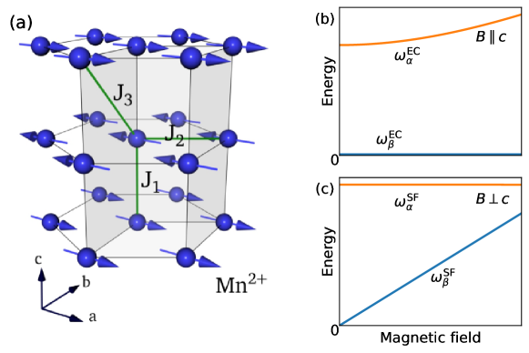
Figure 1: (a) Magnetic structure of $\alpha$-MnTe with ferromagnetic arrangement of Mn²⁺ spins in each hexagonal plane and antiferromagnetic coupling between adjacent planes. The green lines show the exchange coupling terms in Hamiltonian (1), the gray volume marks the magnetic unit cell. Panels (b) and (c) show the theoretically expected $B$-dependence of the $\beta$ and $\alpha$ magnon ($k=0$) modes for the magnetic field applied along and perpendicular to the $c$ axis, respectively. For details see Sec. II.

The dispersion of magnon excitations in $\alpha$-MnTe was mapped by means of inelastic neutron scattering experiments and modeled, using linear spin wave (LSW) theory, by Szuszkiewicz et al. [25]. In their model, they considered an easy-plane type of the antiferromagnetic order and therefore, as is known in NiF₂ [26], the double degeneracy of magnon dispersion is lifted at the center of the magnetic Brillouin zone ($k=0$ magnons). However, experimentally, only a single magnon mode at the energy of $2.6\pm 0.8$ meV ($0.65\pm 0.20$ THz) was resolved at the $\Gamma$ point [25].

In this study, we present antiferromagnetic resonance (AFMR) experiments in the THz spectral range conducted on bulk $\alpha$ -MnTe across a wide range of temperatures and applied magnetic fields. The observed behavior is consistent with theoretical predictions for an easy-plane (hard-axis) antiferromagnet, based on the LSW theory. Our modeling allows us to estimate the out-of-plane anisotropy – the parameter that defines the magnetic properties of MnTe to a great extent. This refines the value reported in the previous study using inelastic neutron scattering [25].

II Theoretical model

The antiferromagnetic resonance is a phenomenon widely explored in solid-state physics, approached theoretically both at the classical and quantum levels [27, 28, 29]. Here we summarize theoretical expectations for the AFMR in an easy-plane antiferromagnet, which can be taken as the first approximation for $\alpha$-MnTe. Hence, we neglect the in-plane anisotropy as well as the (higher-order) Dzyaloshinskii-Moriya interaction which are both relevant for MnTe [6], but they imply energy scales at least one order of magnitude smaller than the out-of-plane anisotropy. Similarly, the proposed model, see Appendix A for details, disregards magnon-magnon interactions. Their inclusion should not lead to a qualitative change in the dispersion of magnons, apart from its broadening [30]. Hence, our model should be sufficient for a description of the dispersion profile.

Let us consider the standard Heisenberg-type Hamiltonian, comprising the exchange interactions up to the third nearest neighbors. It includes the inter-sublattice coupling ($J_{1,3}$) and intra-sublattice coupling ($J_{2}$), cf. Fig. 1a, the single-ion anisotropy ($D>0$), as well as the Zeeman term:

$$\begin{split}\hat{\mathcal{H}}=J_{1}\sum_{{\langle ij\rangle}_{1}}{\bf S}_{i}\cdot{\bf S}_{j}+J_{2}\sum_{{\langle ij\rangle}_{2}}{\bf S}_{i}\cdot{\bf S}_{j}+J_{3}\sum_{{\langle ij\rangle}_{3}}{\bf S}_{i}\cdot{\bf S}_{j}\\ +D\sum_{i}(S_{i}^{z})^{2}-g\mu_{B}\sum_{i}\mathbf{B}\cdot{\mathbf{S}}_{i}\,,\end{split}$$ (1)

where the $z$ direction is parallel to the $c$ axis and spin $S$ reaches 5/2 for Mn²⁺ ions. The magnetic field has a general orientation, and in our approximation of an easy-plane antiferromagnet, we describe it by the angle $\theta_{B}$ between $\mathbf{B}$ and the $c$ axis.

Clearly, the above Hamiltonian implies three distinct energy scales: the Zeeman energy $E_{Z}=g\mu_{B}B$, the magnetic anisotropy energy $E_{\mathrm{an}}=DS$ (due to both the SOC affecting the band structure and the dipole-dipole interaction [31]), and the effective exchange energy $E_{J}=\sum_{n}J_{n}{\cal Z}_{n}S$, where $n$ runs over the neighboring inter-sublattice spins ($n=1$ and 3), with the exchange coupling strength of $J_{n}$ and the corresponding coordination number ${\cal Z}_{n}$ (${\cal Z}_{1}=2$, ${\cal Z}_{3}=12$).

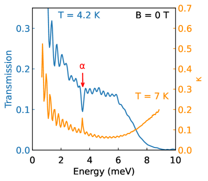
Figure 2: Low-temperature THz transmission spectrum of the bulk $\alpha$-MnTe layer with the thickness of $d=400$ $\mu$m (sample A), measured using the frequency-domain Fourier-transform technique, compared with the extinction coefficient $\kappa$ obtained using the time-domain THz spectroscopy. The vertical arrow indicates the energy of a magnetic excitation identified as the $\alpha$ mode in this work.

The magnon dispersion, including the $k=0$ modes relevant for our optical and magneto-optical experiments, is often obtained using the LSW theory [25, 29]. In antiferromagnets with easy-plane magnetic anisotropy and two spins per unit cell, such as MnTe (see Fig. 1a), we expect the degeneracy of the two magnon modes to be lifted throughout the Brillouin zone. At the $\Gamma$ point, the separation between them scales with the strength of the magnetic anisotropy. At non-zero momenta, interestingly, a part of the splitting may be associated with the altermagnetic nature of MnTe [12, 13]. In the following, we will refer to the lower and upper magnon branches at $k=0$ as the $\beta$ and $\alpha$ modes, respectively.

The LSW theory predicts the energies of both magnon modes, $\hbar\omega_{\alpha}(B)$ and $\hbar\omega_{\beta}(B)$, for any strength and direction of the applied magnetic field. Particularly simple expressions are obtained in two limiting cases: for $\mathbf{B}\perp c$ ($\theta_{B}=\pi/2$), when $B$ exceeds the corresponding spin-flop fields ($B_{\mathrm{sf}}$ below 4 T, see Refs. [24, 32]) and for ${\mathbf{B}}\,\|\,c$ ($\theta_{B}=0$). In the following, we will call these cases “spin-flop” (SF) and “even canting” (EC) configurations, respectively.

In our simplified Hamiltonian for spins in MnTe (1), the $k=0$ magnon energies depend on the applied magnetic field ($E_{Z}\propto B$) as

$$\hbar\omega^{\mathrm{EC}}_{\beta} =0,$$ (2)

$$\hbar\omega^{\mathrm{EC}}_{\alpha} =\sqrt{4E_{\mathrm{an}}E_{J}+\frac{E_{J}E_{Z}^{2}(E_{J}-E_{\mathrm{an}})}{(E_{J}+E_{\mathrm{an}})^{2}}},$$ (3)

for the EC case (for any magnitude of $B$), while in the SF case, we obtain for $B>B_{\mathrm{sf}}$ (but $E_{Z}\leq 2E_{J}$)

$$\hbar\omega^{\mathrm{SF}}_{\beta} =E_{Z}\sqrt{1-\frac{E_{\mathrm{an}}}{E_{J}}},$$ (4)

$$\hbar\omega^{\mathrm{SF}}_{\alpha} =\sqrt{4E_{\mathrm{an}}E_{J}-\frac{E_{\mathrm{an}}E_{Z}^{2}}{E_{J}}}.$$ (5)

At $B=0$, these results agree with Eqs. 23 and 24 of Ref. [29] in the limit of a vanishing in-plane anisotropy. At a non-zero magnetic field, but still below $B_{\mathrm{sf}}$, the energies of magnon modes strongly depend on the initial angle between magnetic moments and the applied (in-plane) magnetic field. This case was treated theoretically [33] and studied experimentally in easy-plane antiferromagnets, e.g., in the recent magneto-Raman scattering experiment on NiPS₃ [34], but it is not relevant for experimental data presented in this work.

In $\alpha$-MnTe, one may expect $E_{J}\gg E_{\mathrm{an}}$ [25, 13] which allows us to plot, in a qualitative way, the expected $B$ dependence of $k=0$ modes, see Fig. 1b,c. In the SF and EC configurations, we find distinctively different behavior. In the EC case, the $\alpha$ mode undergoes a profound blueshift, approximately quadratic at low magnetic fields, while the $\beta$ mode stays at zero, unless effects due to the considerably weaker in-plane anisotropy are considered, see e.g., Ref. [29]. In the SF case, the $\alpha$ mode undergoes a weak redshift with $B$, while the $\beta$ mode approaches the spin resonance of a free electron. Unfortunately, as discussed in the following, only the $\alpha$ mode is observed in our THz experiments.

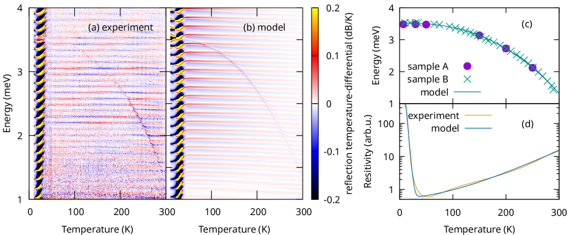
Figure 3: (a) Temperature-differential reflectivity of $\alpha$-MnTe (sample B) as a function of frequency and temperature measured using the time-domain technique, compared with results of the theoretical model (b) explained in the main text and Appendix E. (c) Experimentally determined magnon energy as a function of temperature for samples B and A. Observed decrease in energy is compared with universality class models implying $(T/T_{N})^{\zeta}$ scaling [35]. (d) Electrical resistivity of sample B as a function of $T$ with the theoretical fit described in Appendix E.

III Experimental

Bulk MnTe samples, studied in this work, were prepared in two batches using different growth methods. Sample A was grown using the self-flux technique. Pure manganese (99.9998%) and tellurium (99.9999%) in the molar composition Mn₃₃Te₆₇ were placed in an alumina (99.95%) crucible and, together with a catch crucible filled with quartz wool, sealed in a fused-silica tube under vacuum. The sample was heated up to 1050 ^∘C and then cooled down to 760 ^∘C for four days. At 760 ^∘C, the sample was quickly placed in a centrifuge, separating the crystals from the remaining melt. The crystals were flat plates with lateral dimensions of several millimeters and with the thickness of several hundred of microns. Bulk MnTe crystals grown under identical conditions had been characterized using powder and single-crystal X-ray techniques, magnetic susceptibility measurements, and XPS spectroscopy in Ref. [18].

Sample B was produced by the vapor-solid method. Pure tellurium and manganese powders (99. 999%) were placed at two ends of a quartz ampule, which was sealed under vacuum and heated. After evaporation of tellurium at the temperature of 600 ^∘C, at about 950 ^∘C tellurium vapors reacted with manganese, forming irregular shaped crystals with typical dimensions of several millimeters. The crystals were characterized by X-ray diffraction (both powder and monocrystal one). An equivalent sample had been extensively studied using the electron transport and magnetization methods in Ref. [6].

Four different methods of THz spectroscopy were employed to gather experimental data presented in this paper: (i) Fourier-transform magneto-spectroscopy at low temperatures; (ii) the time-domain technique employed at $B=0$ in a broad range of temperatures with a complementary set of data collected under magnetic field applied at low temperatures; (iii) magnetic-circular-dichroism (MCD) technique at selected THz frequencies and varying temperatures; and (iv) high-frequency electron-spin resonance (ESR). These experimental techniques are described in detail in Appendix D.

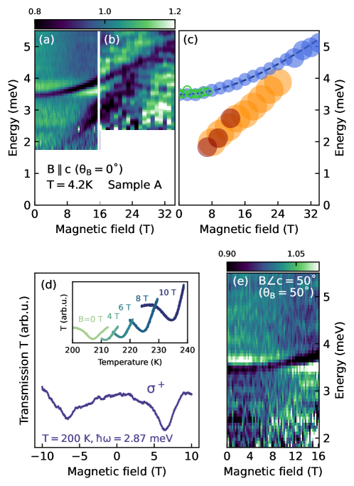
Figure 4: A color map of magneto-transmission taken on sample A at liquid helium temperature using (a) superconducting and (b) resistive coils, with the magnetic field applied along the $c$ axis. The magneto-transmission $T_{B}$ is normalized by the transmission averaged over the whole field range. The extracted positions of resonances with a step of 2 T are plotted as blue circles in (c), complemented with data obtained by the time-domain THz and ESR techniques (green and dark orange circles, respectively), see Appendix F for the latter. The size of the circles corresponds to the error bar. For the dashed line, see the main text. Panel (d) displays the magneto-transmission of sample A, probed by the THz/FIR laser. The magnetic-field sweep at a temperature of $T=200$ K was obtained using circularly polarized radiation with a photon energy of $\hbar\omega=2.87$ meV. The temperature sweeps, shown in the inset, were measured at several magnetic fields using a linearly polarized laser beam with a photon energy of 2.71 meV. Panel (e) shows low-temperature magneto-transmission plotted as a color map, for $B$ applied at the angle of $\theta_{B}=50^{\circ}$ with respect to the $c$ axis.

IV Results and discussion

Let us start the discussion of our experimental results with the transmission spectrum of sample A measured using the Fourier-transform technique at $B=0$ and $T=4.2$ K, see the blue line in Fig. 2. In the THz range, the transmission gradually decreases with photon energy and vanishes above 9 meV due to the onset of the reststrahlen band. In the explored spectral window, the transmission spectrum is weakly modulated by an interference pattern. We observe only a single absorption mode marked by the vertical arrow in Fig. 2. The same excitation is also visible in the extinction coefficient $\kappa$ extracted using the time-domain THz spectroscopy, see the orange line in Fig. 2. As justified a posteriori, by the characteristic temperature and magnetic-field dependence, this is the AFMR signal of MnTe. Equivalently, we may call it the $k=0$ magnon mode that corresponds to the upper dispersion branch ($\alpha$ mode). At low temperatures, the mode has an energy of $E_{\alpha}=\hbar\omega_{\alpha}^{B=0}=(3.5\pm 0.1)$ meV. For comparison, the magnon energy reported for an epitaxial layer of bulk cubic MnTe is larger, reaching nearly 4.3 meV at low temperatures [36, 37].

In Fig. 3a, we present, in the form of a color plot, $T$-differential reflection spectra of sample B, measured using THz time-domain spectroscopy (temperature-differential approach is explained in Appendix D). The characteristic redshift of the magnon mode with $T$ is directly visible in the raw data and we performed a more detailed analysis to extract its spectral position. Apart from the magnon excitation, the studied optical response also depends on free carriers (holes), the dynamics of which display a marked temperature dependence on both the density and scattering rate. The latter is manifested by a pronounced minimum of electrical resistivity (Fig. 3d and Appendix B) at $T\approx 50$ K that coincides with the minimum of optical transmission in the THz spectral range. This minimum separates the low- and high-temperature regimes, where the temperature-driven changes in resistivity are mainly due to the freeze-out of free carriers on shallow acceptor centers and due to thermally activated scattering, respectively. We have modeled this behavior using a simple Drude-type approach which provided us with parameters required for a reliable fit of our THz reflectivity data, see Appendix E.

The extracted positions of the magnon resonance are plotted in Fig. 3b, complemented by several control points obtained on sample A using an independent time-domain THz setup. With increasing $T$, the observed mode exhibits a pronounced redshift, down to 1.4 meV at room temperature. Such a redshift is characteristic of magnon excitations in magnetic materials when approaching, from below, the ordering temperature, see, e.g., Refs. [38, 39]. In Fig. 3b, we modeled this behavior using the formula $E_{\alpha}(T)=E_{\alpha}[1-c(T/T_{N})^{\zeta}]$, with $\zeta$ and $c$ as the fitting parameters. Consistent with Refs. [40, 35], this yielded values of $\zeta=(2.5\pm 0.1)$ and $c=(0.68\pm 0.05)$.

Our optical measurements on $\alpha$-MnTe in an external magnetic field are summarized in Fig. 4. The basic set of the collected data, with $\mathbf{B}$ applied along the $c$ axis of MnTe (EC configuration) is presented in panel (a). The observed magnetic excitation, exhibiting a pronounced blueshift, approximately quadratic in $B$, can be directly associated with the $\alpha$ mode. Despite a lower signal-to-noise ratio, the monotonic blueshift is well visible also in the high-field part of the data, see panel (b), and continues up to the highest magnetic field applied (33 T). The extracted energies of the $\alpha$ mode are plotted in panel (c) together with the low-field points obtained using the time-domain THz spectroscopy and ESR techniques.

Interestingly, another field-dependent spectral feature emerges at lower photon energies, see Figs. 4a and b and orange circles in Fig. 4c. One could invoke the possibility that this extra line is the lower magnon branch ($\beta$ mode). In fact, also the $\beta$ mode may acquire a non-zero energy and gain a non-trivial dependence on $B$ when the in-plane component of anisotropy is not fully negligible. However, a closer inspection of our data collected on other MnTe samples from batch A excludes this scenario. In contrast to the $\alpha$ line, which is consistently present in all our measurements, the lower energy line is not manifested in all samples. Presumably, this reflects the varying hole density among the samples studied. In addition, the lower-energy line broadens significantly with $B$. This is considerably different from behaviour of the $\alpha$ line and represents another argument against the magnon origin of this extra line.

To find an interpretation for this extra line, let us recall the nearly linear dependence of its position on the applied magnetic field, see Fig. 4c. This may remind us of conventional cyclotron resonance (CR) of free charge carriers [41]. However, at the same time, the zero-field extrapolation yields a nonzero energy. Such behavior was observed in previous CR studies of weakly bound electrons in bulk semiconductors and their heterostructures, see, e.g., Refs. [42, 43, 44, 45]. In fact, the presence of electrons localized at low temperatures is consistent with a sharp drop in electrical resistance observed with increasing $T$, see Fig. 5. The slope of the extra line would imply a rather high effective mass, $m_{\mathrm{eff}}\approx m_{0}$. This is, however, greater than the previously reported experimental values ($\approx 0.25m_{0}$ confirmed also by ab initio calculations, see Sec. 2 of the Supplementary information in Ref. [21]) based on zero-field optical studies at liquid nitrogen temperature [46, 47].

Let us now turn back to the $\alpha$ mode (Figs. 4a-c) and examine its other experimentally probed characteristics, the partial circular polarization at $B>0$, see Fig. 4d. It was observed using the THz MCD technique, which operates at a fixed laser frequency with a well-defined circular polarization, and follows the intensity of the transmitted radiation as a function of $B$. The partial circular polarization of the $\alpha$ mode is manifested by a profound difference in the observed absorption when the light propagates parallel or antiparallel to the direction of the magnetic field.

Magnetic circular dichroism in MnTe is a complex phenomenon, sensitive to particular symmetries present (or broken), see, e.g. Ref. [7], nevertheless, the partial circular polarization of the $\alpha$ mode at $B>0$ can be seen just as an effect of the $B$-induced magnetization. In the ${\mathbf{B}}\|c$ configuration, this appears due to spin canting away from the hexagonal plane (the EC regime). The angle between the spin and hexagonal planes reaches a few degrees in the highest applied $B$, $\arcsin[E_{Z}/(2E_{J})]$ (6), for the expected strength of the exchange coupling [25]. Note that the experiment with circularly polarized radiation was performed at higher temperatures ($T=200$ K) at which it was possible to achieve resonance between the field-dependent $\alpha$ mode and one of the (discrete) emission lines of the gas laser. This temperature-driven tuning of the magnon energy, at several values of the magnetic field, is demonstrated in the inset of Fig. 4d.

Let us now compare the magnetic-field dependence of the $\alpha$ mode energy with the proposed theoretical model. The observed blueshift, approximately quadratic in $B$, matches well the expectations raised by Eq. 3 in the limit of a relatively weak magnetic field. The validity of the theoretical model can be further corroborated using an additional set of data collected at various angles $\theta_{B}$ between $\mathbf{B}$ and the $c$ axis. Theoretically, we expect a weakening of the blueshift with increasing $\theta_{B}$, to gradually approach Eq. 5 with a nearly vanishing $B$-dependence for $E_{\mathrm{an}}\ll E_{J}$. Experimentally, we have indeed found that the blueshift of the $\alpha$ mode gradually flattens with increasing $\theta_{B}$. We illustrate this in Fig. 4e on the set of data collected at $\theta_{B}=50^{\circ}$. The complete set of data collected at various angles $\theta_{B}$ is presented in the Appendix C.

Having confirmed the validity of our model at the qualitative level, let us proceed with a quantitative analysis. Knowing the energy of the $\alpha$ mode at $B=0$, as well as its blueshift in the EC configuration, Eq. 3 seems to be sufficient to extract both magnetic anisotropy and effective exchange coupling. However, a closer inspection reveals that for a weak magnetic anisotropy, $E_{\mathrm{an}}\ll E_{J}$, a particular choice of $E_{J}$ and $E_{\mathrm{a}n}$ parameters leads only to a minor correction of the blueshift which becomes dominantly driven by the Zeeman energy $E_{Z}$ and the corresponding $g$ factor in it.

To account for this, we have fitted the experimentally observed blueshift, see the dashed line in Fig. 4c, using the formula $(E_{\alpha}^{2}+\xi^{2}\mu_{B}^{2}B^{2})^{1/2}$, cf. Eq. 3. The extracted parameter $\xi=1.99\pm 0.03$ then allows us to calculate an approximate effective relation between the magnetic anisotropy and the factor $g$: $D\approx(\sqrt{3}E_{\alpha}/15)\sqrt{1-\xi^{2}/g^{2}}$. It is also worth noting that the parameter $\xi$ corresponds to the lowest possible value of the $g$ factor consistent with our magneto-optical data. SOC in Mn-based compounds is typically weak and the effective $g$ factor should not significantly deviate from 2. Setting the maximum value at $g=2.1$, we get the following upper limit for the out-of-plane magnetic anisotropy, $D<150$ $\mu$eV.

Another independent estimate of magnetic anisotropy can be obtained thanks to the AFMR experiment in the SF configuration (${\mathbf{B}}\perp c$). There, the $\alpha$ mode is expected to redshift approximately by $2(g\mu_{B}BD)^{2}/E^{3}_{\alpha}$ as one can infer from Eq. 5. Since no such shift was observed experimentally, we conclude it to be smaller than our experimental resolution (0.5 cm^-1 @ 16 T). In this way, we obtain the upper bound for the magnetic anisotropy: $D<250$ $\mu$eV. This estimate is less strict, but consistent with the one based on our AFMR experiments in the EC configuration.

Using exchange parameters available in the literature for $\alpha$-MnTe we arrive at another way to obtain an estimate of the magnetic anisotropy. Szuszkiewicz et al. [25] mapped the magnon dispersion using inelastic neutron scattering and compared their results with the dispersion obtained by the LSW theory, considering a spin Hamiltonian equivalent to Eq. (1). They found good agreement with the theory, except for small departures around zone boundaries, and gave solid estimates of the corresponding exchange coupling constants. However, magnetic anisotropy seems to be the least precise parameter deduced, mainly due to the limited data set around $k=0$. Combining the exchange parameters $J_{1}$ and $J_{3}$ from Szuszkiewicz et al. [25] leads to $E_{J}\approx 33$ meV (this is essentially the magnon bandwidth seen in Fig. 5 of that reference) and using the $\alpha$ mode energy deduced from the optical measurements in this work (see Fig. 2), we conclude that the out-of-plane component of the magnetic anisotropy falls within $D=40\pm 10$ $\mu$eV [$E_{\mathrm{an}}=100\pm 25$ $\mu$eV]. This, in turn, allows us to estimate the effective $g$ factor, $g=2.03\pm 0.01$, using the AFMR data collected in the EC configuration, see the discussion above.

V Conclusions

A long-wavelength ($k=0$) magnon mode was identified in the THz response of bulk MnTe using the experimentally observed dependence of its energy on the applied magnetic field and temperature. The observed behavior aligns well with predictions from a simplified model of an easy-plane (hard-axis) antiferromagnet, developed within the framework of linear spin-wave theory. Its energy at low temperatures, 3.5 meV, ranks MnTe among antiferromagnetic materials with moderate magnon gap (smaller than in some uniaxial systems [48, 49] but still appreciable). On the other hand, the magnon remains observable even at room temperature which is close to $T_{N}$ of hexagonal MnTe. Combining our experimental results with the values of the exchange parameters published earlier, we determined the out-of-plane component of the magnetic anisotropy as $D=40\pm 10$ $\mu$eV and the effective $g$ factor as $g=2.03\pm 0.01$.

Appendix A Linear spin wave theory

The classical ground state configuration has to be determined first. Writing the classical energy ${\cal E}$ associated with the Hamiltonian (1) we get for $\mathcal{E}/S$

$$E_{J}\mathbf{m}_{1}\cdot\mathbf{m}_{2}+E_{\mathrm{an}}\left[(\mathbf{z}\cdot\mathbf{m}_{1})^{2}+(\mathbf{z}\cdot\mathbf{m}_{2})^{2}\right]-E_{Z}\mathbf{b}\cdot(\mathbf{m}_{1}+\mathbf{m}_{2}),$$

where $\mathbf{m}_{i}$ denote unit vectors corresponding to the respective sublattice magnetizations. The external magnetic field is $\mathbf{B}=\mathbf{b}B$, and without loss of generality, the unit vector $\mathbf{b}$ is taken to be in the plane $\{\mathbf{x},\mathbf{z}\}$. The quantities $E_{\mathrm{an}}$, $E_{Z}$ and $E_{J}$ are defined in the main text.

Minimizing ${\cal E}$, we obtain for $E_{Z}\leq 2E_{J}$ a “canted spin-flop” configuration with polar angle $\theta$, shared by both sublattices, and azimuthal angle $\phi$ taken from $\mathbf{x}$-axis as: $\phi_{1}=-\phi_{2}=\phi:$

$$\cos\theta =\frac{E_{Z}\cos\theta_{B}}{2\left(E_{J}+E_{\mathrm{an}}\right)}\approx\frac{E_{Z}\cos\theta_{B}}{2E_{J}}$$ (6)

$$\cos\phi =\frac{E_{Z}\sin\theta_{B}}{2E_{J}\sin\theta}.$$

We express spin operators in the quantum spin Hamiltonian (1) in their respective sublattice basis $S^{sl}$, such that $S^{sl,z}_{li}=\mathbf{S}_{li}\cdot\mathbf{z}^{sl}_{l}$, with $\mathbf{z}^{sl}_{l}=\mathbf{m}_{l}$ and these operators are then mapped to the bosonic annihilation and creation operators via Holstein-Primakoff transformation (in its semiclassical limit):

$$S^{sl,+}_{1i}\stackrel{{\scriptstyle S\gg 1}}{{\approx}}(2S)^{1/2}a_{i},\quad S^{sl,-}_{1i}\stackrel{{\scriptstyle S\gg 1}}{{\approx}}(2S)^{1/2}a^{\dagger}_{i},$$

$$S^{z}_{1i}=S-a_{i}^{\dagger}a_{i},$$

and similarly for the second sublattice $S^{sl}_{2i}\rightarrow b_{i}^{\dagger},b_{i}$. Only terms quadratic in bosonic operators are taken into account within the LSW theory, i.e., all terms with three or more operators are neglected (single operator terms do not have any effect on the resulting magnon energies). The Fourier-transformed magnon operators $a_{k},a_{k}^{\dagger}$ allow us to write a quadratic Hamiltonian ${\cal H}_{ab}$ comprising four terms.

$$\sum_{\mathbf{k}}A_{\mathbf{k}} (a^{\dagger}_{\mathbf{k}}a_{\mathbf{k}}+b^{\dagger}_{\mathbf{k}}b_{\mathbf{k}})+B_{\mathbf{k}}(a_{\mathbf{k}}b_{-\mathbf{k}}+a^{\dagger}_{\mathbf{k}}b^{\dagger}_{-\mathbf{k}})+$$

$$+ \left[\frac{1}{2}C_{\mathbf{k}}(a_{\mathbf{k}}a_{-\mathbf{k}}+b_{\mathbf{k}}b_{-\mathbf{k}})+h.c.\right]+\left[D_{\mathbf{k}}a^{\dagger}_{\mathbf{k}}b_{\mathbf{k}}+h.c.\right].$$

Here we introduce the following abbreviations

$$A_{\mathbf{k}} =E_{Z}(\cos\theta\cos\theta_{B}+\sin\theta\cos\phi\sin\theta_{B})$$

$$-E_{\mathrm{an}}\frac{1}{2}(1+3\cos 2\theta)-\sum_{n_{i}}E_{j}^{n_{i}}(1-\gamma_{\mathbf{k}}^{n_{i}})$$

$$-\sum_{n_{c}}E_{j}^{n_{c}}(\cos^{2}\theta+\cos 2\phi\sin^{2}\theta)$$

$$B_{\mathbf{k}} =\sum_{n_{c}}E_{j}^{n_{c}}\sin^{2}\theta\sin^{2}\phi\gamma_{\mathbf{k}}^{n_{c}}$$

$$C_{\mathbf{k}} =E_{\mathrm{an}}e^{2i\phi}\sin^{2}\theta$$

$$D_{\mathbf{k}} =\sum_{n_{c}}E_{j}^{n_{c}}e^{2i\phi}(\cos\phi-i\cos\theta\sin\phi)^{2}\gamma_{\mathbf{k}}^{n_{c}}$$

where

$$E_{j}^{n}=J_{n}{\cal{Z}}_{n}S,\ \gamma_{\mathbf{k}}^{n}={\cal{Z}}_{n}^{-1}\sum_{j_{n}}e^{i\mathbf{k}\cdot\mathbf{r}_{j_{n}}},$$

with $n\in\{n_{c},n_{i}\}$ and $n_{i}$ indexing intra-sublattice (within one hexagonal plane) and $n_{c}$ inter-sublattice exchange parameters $J_{n}$, ${\cal{Z}}_{n}$. Note that $E_{J}=\sum_{n_{c}}E_{j}^{n_{c}}.$

Using Bogoliubov transformation to diagonalize $\mathcal{H}_{ab}$

$$\mathcal{H}_{ab}\stackrel{{\scriptstyle BT}}{{\longrightarrow}}\mathcal{H}_{\alpha\beta}=\sum_{\mathbf{k}}\omega_{\alpha\mathbf{k}}\alpha^{\dagger}_{\mathbf{k}}\alpha_{\mathbf{k}}+\omega_{\beta\mathbf{k}}\beta^{\dagger}_{\mathbf{k}}\beta_{\mathbf{k}}$$

we arrive, in the end, at

$$\omega_{\beta/\alpha,\mathbf{k}}^{2} =A_{\mathbf{k}}^{2}-B_{\mathbf{k}}^{2}-|C_{\mathbf{k}}|^{2}+|D_{\mathbf{k}}|^{2}\mp\sqrt{4|E|_{\mathbf{k}}^{2}+F_{\mathbf{k}}^{2}},$$

$$E_{\mathbf{k}} =B_{\mathbf{k}}C_{\mathbf{k}}-A_{\mathbf{k}}D_{\mathbf{k}},\quad F_{\mathbf{k}}=C_{\mathbf{k}}D_{\mathbf{k}}^{*}-C_{\mathbf{k}}^{*}D_{\mathbf{k}}.$$

Setting $k=0$ and appropriate $\mathbf{B}$ (out-of-plane or in-plane), we recover Eqs. (2,3) for $\theta_{B}=0$ and Eqs. (4,5) for $\theta_{B}=\pi/2$. This derivation largely follows Ref. [29].

Appendix B Temperature dependence of electrical resistivity

The temperature dependence of the electrical resistivity for samples A and B is plotted in Fig. 5. Qualitatively, both samples show the same behaviour with increasing $T$. A sharp decrease in resistance, with the minima below 100 K, and a gradual increase at higher temperatures. At high temperatures, the resistance of sample B appears to be approximately one order of magnitude higher than that of sample A. Assuming that the scattering of free carriers at high temperatures is dominated by intrinsic mechanisms (optical phonons), the difference in the resistance values may suggest a higher carrier density in sample A.

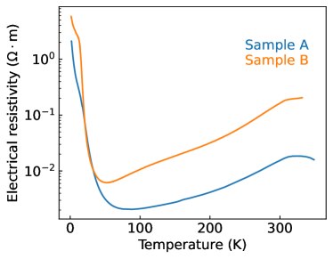
Figure 5: Resistivity dependence on temperature for samples A and B with carrier freeze-out evidenced at low temperatures. The experiments were carried out using the conventional lock-in technique at low frequencies. The profile of $R(T)$ curve qualitatively match overall transmission of MnTe samples in the THz range, as discussed in the main text.

Appendix C Magneto-transmission of $\alpha$-MnTe –
a complementary set of data

An additional set of magneto-transmission data collected in the Faraday configuration on sample A using the frequency-domain spectroscopy, with the magnetic field applied at different angles $\theta_{B}$ with respect to the $c$ axis of MnTe, is plotted in Fig. 6. This set of data illustrates the relatively weak sensitivity of the $\alpha$ mode to the in-plane component of the applied magnetic field, in line with the expectations of the theoretical model (Sect. II and Appendix A). The blue shift of the $\alpha$ mode induced by the magnetic field, well-pronounced at low angles $\theta_{B}$, becomes at the limit of our experimental resolution above $\theta_{B}=60^{\circ}$. At higher angles, no blueshift was observed, including the limiting case of $\theta_{B}=90^{\circ}$ which we probed in the Voigt configuration (data not presented).

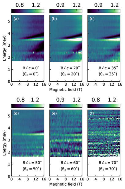
Figure 6: Relative magneto-transmission, $T_{B}/T_{B=0}$ collected in the Faraday configuration on sample A at liquid helium temperature, plotted as color plots for several values of the angle between the magnetic field and the $c$ axis of MnTe: $\theta_{B}=0,20,35,50,60$ and 70^∘ in panels (a) to (f). The data in panels (a) and (d) are the same as in Figs. 4a and e, but this time normalized by the zero-field transmission. In this way, the dark and light colors correspond to areas of $B$-induced absorption and transmission, respectively.

Appendix D Description of experimental techniques

Fourier transform magneto-spectroscopy: Nonpolarized radiation from mercury lamp was analyzed by the Bruker Vertex 80v spectrometer and delivered, via light-pipe optics, to the sample which was kept at $T=4.2$ K in the helium exchange gas and placed inside a cryostat in a superconducting or resistive coil, below and above 16 T, respectively. In the superconducting coil, the radiation was then detected by a composite bolometer placed just below the sample. In this case, both Faraday and Voigt configurations were possible, with the light propagating along or perpendicular to the applied magnetic field, respectively. In the resistive coil, measurements were made only in the Faraday configuration. In order to reduce the noise level induced by the cooling water, the sample was placed on a mirror and the radiation was detected by an external bolometer. The signal in this latter configuration corresponds to a double-pass transmission. For the absolute transmission measurement in Fig. 2, the sample was mounted on a rotation stage that enabled referencing by an open aperture.

Time-domain THz spectroscopy: Experiments using this method were carried out in reflection and transmission geometries. Reflection measurements, performed on sample B, were performed at an incidence angle of 11^∘, using a THz optical setup with four off-axis parabolic mirrors. We used a photoconductive source and detector antennae, controlled with a standard THz time-domain spectrometer (Toptica). The sample was placed in an optical cryostat with quartz windows, and reflection spectra were collected as a function of the sample temperature in the range of 10-300 K. We calculated temperature-differential reflection spectra that show the $\alpha$ magnon mode because its frequency softens with increasing temperature. These spectra reveal strong interactions of the magnon with the modes of a Fabry-Perot cavity, formed due to the parallel-plane shape of the sample [50]. Due to a relatively large sample B thickness (989 $\mu$m), the cavity modes are dense in the frequency domain.

The time-domain THz experiments in the transmission geometry were performed in two custom-made THz setups. For measurements without magnetic field, broadband pulses (0.2-3 THz) were generated by a photoconducting antenna and detected by electro-optic sampling in a ZnTe crystal. The sample was cooled in an optical cryostat (Optistat, Oxford instruments) from 300 down to 7 K. For more details on the setup, see Ref. [51]. For measurements in a magnetic field, broadband terahertz pulses were generated and detected using commercial fiber-coupled photoconductive switches operating with a femtosecond optical fiber laser system (TeraSmart, Menlo Systems GmbH). The sample was placed in an Oxford Instruments Spectromag He bath cryostat fitted with mylar windows and a superconducting coil, allowing for applying a magnetic field of up to 7 T, and cooling the sample down to 2 K. The measurements were performed in the Faraday geometry.

THz magnetic-circular dichroism (THz-MCD): Temperature and magnetic-field-dependent transmittance measurements with a circularly polarized THz beam were performed in the Faraday geometry. The optically pumped THz/FIR gas laser (Edinburgh Instruments FIRL100) produced a highly monochromatic, linearly polarized THz beam, which was converted into a left-handed or right-handed circularly polarized state using a broadband tunable terahertz retarder [52]. The cyclotron resonance absorption of a high-quality two-dimensional electron gas in the GaAs quantum well is measured to ensure pure circular polarization. The magneto-optical cryogenic system (Oxford Instruments Spectromag SM4000) provides temperatures from 2 to 300 K and magnetic fields up to 10 T in both polarities. The relative transmittance is given as a ratio of the signal transmitted through the sample and detected by a liquid-helium-cooled bolometer to the signal monitoring the laser output. An additional set of data (see the inset of Fig. 4d) was collected using the described setup, but with linearly polarized radiation instead, to illustrate the fine tuning of the $\alpha$ magnon energy with $T$.

High-field high-frequency electron spin resonance (ESR): The explored sample was placed in an open cavity, in the Faraday configuration, in a superconducting coil and kept at low temperatures ($T=5$ K) in the variable temperature insert. The quasi-monochromatic radiation ($\hbar\omega=1.8$, 2.1 and 2.7 meV were used) was generated via an amplification-multiplication chain of a basic 9.2 GHz synthesized frequency and delivered to the sample by means of quasi-optics. The magnetic-field-modulation technique was employed. The double-transmitted radiation was detected by an external bolometer. For more details, see Ref. [53].

Appendix E Modeling of time-domain THz data

The reflection spectra obtained by the time-domain technique were modeled using the transfer matrix formalism [54]. Following the experimental configuration used, we considered a plane-parallel slab of MnTe (the thickness of 989 $\mu$m) placed on a highly reflective metallic layer. The dielectric part of the optical response was described as $\epsilon=\epsilon_{bg}[1-\omega_{p}^{2}/(\omega^{2}+i\omega\gamma_{p})]$, where $\omega_{p}=[Ne^{2}/(\epsilon_{0}\epsilon_{\mathrm{bg}}m_{\mathrm{eff}})]^{1/2}$ is the screened plasma frequency. It describes the response due to free carriers (holes) with the density $N$, effective mass $m_{\mathrm{eff}}$, and scattering rate $\gamma_{p}$. To describe the magnon resonance, the magnetic susceptibility was expressed using a Lorentz-type model, $\mu=1+\chi\omega_{m}^{2}/(\omega_{m}^{2}-\omega^{2}-i\omega_{m}\gamma_{m})$, where $\chi$ stands for the oscillator strength of the AFMR, $\omega_{m}$ is the magnon energy and $\gamma_{m}$ is the AFMR line width.

To reduce the number of free-fitting parameters, the effective mass was set to the mass of a bare electron ($m_{\mathrm{eff}}=m_{0}$). Then, we analyzed the temperature dependence of the electrical resistivity (Fig. 3d) to get estimates for $N(T)$ and $\gamma_{p}(T)$. To this end, we fitted the profile of electrical resistivity using an empirical formula, $R(T)=a(1+be^{T/T_{b}})(1+ce^{-T/T_{c}})$. With increasing $T$, this formula describes reasonably well (see the solid line in Fig. 3d) the initial rapid drop in resistivity due to the sharply increasing hole density, which is followed, above $T\approx 50$ K, by a gradual increase in resistivity, driven by the decreasing mobility of the holes. To separate the contributions of the carrier density and the scattering rate to the temperature dependence of (Drude-type) electrical resistivity, $\rho=m_{\mathrm{eff}}\gamma_{p}/(Ne^{2})$, the carrier density at $T=50$ K was anchored at $N=5\times 10^{16}$ cm^-3 – the value typically observed in Hall experiments in explored MnTe samples.

In addition to the temperature dependence of the magnon energy, presented and modeled in the main text (Fig. 3c), our fitting procedure also provided us with the width and strength of the AFMR, including their temperature dependencies. The width appeared well reproduced by the effective formula: $\gamma_{m}=\gamma_{m}^{0}(1+T[K]/300)$, where $\gamma_{m}^{0}=40$ $\mu$eV. Regarding oscillator strength, it was highest around 10 K and weakened rapidly with $T$. The magnon excitations became barely observable in the temperature range 50-100 K, but the strength then gradually increased at higher temperatures. This behavior can be traced directly in the bare data set (Fig. 3a) through the splitting of the magnon-polariton modes at the crossing of the AFMR with subsequent modes of the Fabry-Perot modes of the cavity formed by the sample slab. The Rabi splitting is proportional to $\sqrt{\chi}$. The Fabry-Perot pattern also allowed us to firmly determine the background dielectric function that varies smoothly with $T$, $\epsilon_{\mathrm{bg}}(T)=20.5+i0.08+2.0\cdot 10^{-3}(1+i)T[\mathrm{K}]$.

Appendix F High-field high-frequency electron spin resonance - dataset

A complementary experiment was carried out on sample A using the ESR technique. The experimental data collected at $T=5$ K are plotted in Fig. 7. There, we plot the MnTe microwave transmission as a function of the applied magnetic field at three selected microwave frequencies ($\hbar\omega=1.8,2.1$ and 2.7 meV), in the form of $B$-derivatives. Vertical dashed lines mark the positions of the relevant resonances.

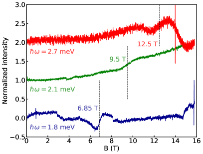
Figure 7: Dataset of $B$-derivative of magneto-transmission measured by the ESR technique. The extracted resonance positions, see vertical dashed lines with labels, are shown as dark orange points in Fig.4c.

References

- Allen et al. [1977] J. Allen, G. Lucovsky, and J. Mikkelsen, Optical properties and electronic structure of crossroads material MnTe, Solid State Commun. 24, 367 (1977).
- Mu et al. [2019] S. Mu, R. P. Hermann, S. Gorsse, H. Zhao, M. E. Manley, R. S. Fishman, and L. Lindsay, Phonons, magnons, and lattice thermal transport in antiferromagnetic semiconductor MnTe, Phys. Rev. Mater. 3, 025403 (2019).
- Baltz et al. [2018] V. Baltz, A. Manchon, M. Tsoi, T. Moriyama, T. Ono, and Y. Tserkovnyak, Antiferromagnetic spintronics, Rev. Mod. Phys. 90, 015005 (2018).
- Kriegner et al. [2016] D. Kriegner, K. Výborný, K. Olejník, H. Reichlová, V. Novák, X. Marti, J. Gazquez, V. Saidl, P. Němec, V. V. Volobuev, G. Springholz, V. Holý, and T. Jungwirth, Multiple-stable anisotropic magnetoresistance memory in antiferromagnetic MnTe, Nat. Commun. 7, 11623 (2016).
- Kriegner et al. [2017a] D. Kriegner, H. Reichlova, J. Grenzer, W. Schmidt, E. Ressouche, J. Godinho, T. Wagner, S. Y. Martin, A. B. Shick, V. V. Volobuev, G. Springholz, V. Holý, J. Wunderlich, T. Jungwirth, and K. Výborný, Magnetic anisotropy in antiferromagnetic hexagonal MnTe, Phys. Rev. B 96, 214418 (2017a).
- Kluczyk et al. [2024] K. P. Kluczyk, K. Gas, M. J. Grzybowski, P. Skupiński, M. A. Borysiewicz, T. Fas, J. Suffczyński, J. Z. Domagala, K. Grasza, A. Mycielski, M. Baj, K. H. Ahn, K. Výborný, M. Sawicki, and M. Gryglas-Borysiewicz, Coexistence of anomalous Hall effect and weak magnetization in a nominally collinear antiferromagnet MnTe, Phys. Rev. B 110, 155201 (2024).
- [7] M. Hubert, T. Malecek, K.-H. Ahn, M. Misek, J. Zelezny, F. Maca, G. Springholz, M. Veis, and K. Vyborny, Anomalous spectroscopical effects in an antiferromagnetic semiconductor: The case of magneto-optical Kerr effect, phys. stat. sol. (b) , 2400541.
- Hariki et al. [2024] A. Hariki, A. Dal Din, O. J. Amin, T. Yamaguchi, A. Badura, D. Kriegner, K. W. Edmonds, R. P. Campion, P. Wadley, D. Backes, L. S. I. Veiga, S. S. Dhesi, G. Springholz, L. Šmejkal, K. Výborný, T. Jungwirth, and J. Kuneš, X-ray magnetic circular dichroism in altermagnetic -MnTe, Phys. Rev. Lett. 132, 176701 (2024).
- Gonzalez Betancourt et al. [2024] R. D. Gonzalez Betancourt, J. Zubáč, K. Geishendorf, P. Ritzinger, B. Růžičková, T. Kotte, J. Železný, K. Olejník, G. Springholz, B. Büchner, A. Thomas, K. Výborný, T. Jungwirth, H. Reichlová, and D. Kriegner, Anisotropic magnetoresistance in altermagnetic MnTe, npj Spintronics 2, 45 (2024).
- Nagaosa et al. [2010] N. Nagaosa, J. Sinova, S. Onoda, A. H. MacDonald, and N. P. Ong, Anomalous Hall effect, Rev. Mod. Phys. 82, 1539 (2010).
- Ritzinger and Vyborny [2023] P. Ritzinger and K. Vyborny, Anisotropic magnetoresistance: materials, models and applications, R. Soc. Open Sci. 10, 230564 (2023).
- Šmejkal et al. [2023] L. Šmejkal, A. Marmodoro, K.-H. Ahn, R. González-Hernández, I. Turek, S. Mankovsky, H. Ebert, S. W. D’Souza, O. Šipr, J. Sinova, and T. Jungwirth, Chiral magnons in altermagnetic , Phys. Rev. Lett. 131, 256703 (2023).
- Liu et al. [2024] Z. Liu, M. Ozeki, S. Asai, S. Itoh, and T. Masuda, Chiral split magnon in altermagnetic MnTe, Phys. Rev. Lett. 133, 156702 (2024).
- Šmejkal et al. [2022a] L. Šmejkal, J. Sinova, and T. Jungwirth, Beyond conventional ferromagnetism and antiferromagnetism: A phase with nonrelativistic spin and crystal rotation symmetry, Phys. Rev. X 12, 031042 (2022a).
- Šmejkal et al. [2022b] L. Šmejkal, J. Sinova, and T. Jungwirth, Emerging research landscape of altermagnetism, Phys. Rev. X 12, 040501 (2022b).
- Liu et al. [2025] Liu, Dai, and Blügel, Different facets of unconventional magnetism, Nature Phys. 10.1038/s41567-024-02750-3 (2025).
- Note [1] Combined spatial and time inversion . In addition to this symmetry, translations combined with also have to be absent among the symmetries. It should be stressed that non-collinear magnets can, of course, also have broken symmetry.
- Krempaský et al. [2024] J. Krempaský, L. Šmejkal, S. W. D’Souza, M. Hajlaoui, G. Springholz, K. Uhlířová, F. Alarab, P. C. Constantinou, V. Strocov, D. Usanov, W. R. Pudelko, R. González-Hernández, A. Birk Hellenes, Z. Jansa, H. Reichlová, Z. Šobáň, R. D. Gonzalez Betancourt, P. Wadley, J. Sinova, D. Kriegner, J. Minár, J. H. Dil, and T. Jungwirth, Altermagnetic lifting of Kramers spin degeneracy, Nature 626, 517 (2024).
- Osumi et al. [2024] T. Osumi, S. Souma, T. Aoyama, K. Yamauchi, A. Honma, K. Nakayama, T. Takahashi, K. Ohgushi, and T. Sato, Observation of a giant band splitting in altermagnetic mnte, Phys. Rev. B 109, 115102 (2024).
- Ferrer-Roca et al. [2000] C. Ferrer-Roca, A. Segura, C. Reig, and V. Muñoz, Temperature and pressure dependence of the optical absorption in hexagonal MnTe, Phys. Rev. B 61, 13679 (2000).
- Faria Junior et al. [2023] P. E. Faria Junior, K. A. de Mare, K. Zollner, K.-h. Ahn, S. I. Erlingsson, M. van Schilfgaarde, and K. Výborný, Sensitivity of the MnTe valence band to the orientation of magnetic moments, Phys. Rev. B 107, L100417 (2023).
- Madelung et al. [2000] O. Madelung, U. Rössler, and M. Schulz, Non-Tetrahedrally Bonded Binary Compounds II: Supplement to Vol. III/17g (Print Version) Revised and Updated Edition of Vol. III/17g (CD-ROM). (Springer, 2000).
- Komatsubara et al. [1963] T. Komatsubara, M. Murakami, and E. Hirahara, Magnetic properties of manganese telluride single crystals, J. Phys. Soc. Jpn. 18, 356 (1963).
- Kriegner et al. [2017b] D. Kriegner, H. Reichlova, J. Grenzer, W. Schmidt, E. Ressouche, J. Godinho, T. Wagner, S. Y. Martin, A. B. Shick, V. V. Volobuev, G. Springholz, V. Holý, J. Wunderlich, T. Jungwirth, and K. Výborný, Magnetic anisotropy in antiferromagnetic hexagonal MnTe, Phys. Rev. B 96, 214418 (2017b).
- Szuszkiewicz et al. [2006] W. Szuszkiewicz, E. Dynowska, B. Witkowska, and B. Hennion, Spin-wave measurements on hexagonal of -type structure by inelastic neutron scattering, Phys. Rev. B 73, 104403 (2006).
- Moriya [1960] T. Moriya, Theory of magnetism of Ni, Phys. Rev. 117, 635 (1960).
- Kittel [1951] C. Kittel, Theory of antiferromagnetic resonance, Phys. Rev. 82, 565 (1951).
- Keffer and Kittel [1952] F. Keffer and C. Kittel, Theory of antiferromagnetic resonance, Phys. Rev. 85, 329 (1952).
- Rezende et al. [2019] S. M. Rezende, A. Azevedo, and R. L. Rodriguez-Suarez, Introduction to antiferromagnetic magnons, J. Appl. Phys. 126, 151101 (2019).
- Garcia-Gaitan et al. [2025] F. Garcia-Gaitan, A. Kefayati, J. Q. Xiao, and B. K. Nikolić, Magnon spectrum of altermagnets beyond linear spin wave theory: Magnon-magnon interactions via time-dependent matrix product states versus atomistic spin dynamics, Phys. Rev. B 111, L020407 (2025).
- Corrêa and Výborný [2018] C. A. Corrêa and K. Výborný, Electronic structure and magnetic anisotropies of antiferromagnetic transition-metal difluorides, Phys. Rev. B 97, 235111 (2018).
- Bey et al. [2024] S. Bey, S. S. Fields, N. G. Combs, B. G. Markus, D. Beke, J. Wang, A. V. Ievlev, M. Zhukovskyi, T. Orlova, L. Forro, S. P. Bennett, X. Liu, and B. A. Assaf, Unexpected tuning of the anomalous Hall effect in altermagnetic MnTe thin films (2024), arXiv:2409.04567 [cond-mat.mtrl-sci] .
- T. Nagamiya and Kubo [1955] K. Y. T. Nagamiya and R. Kubo, Antiferromagnetism, Adv. Phys. 4, 1 (1955).
- Jana et al. [2023] D. Jana, P. Kapuscinski, I. Mohelsky, D. Vaclavkova, I. Breslavetz, M. Orlita, C. Faugeras, and M. Potemski, Magnon gap excitations and spin-entangled optical transition in the van der Waals antiferromagnet , Phys. Rev. B 108, 115149 (2023).
- Köbler and Hoser [2010] U. Köbler and A. Hoser, Renormalization group theory: impact on experimental magnetism, Vol. 127 (Springer Science & Business Media, 2010).
- Szuszkiewicz et al. [1997] W. Szuszkiewicz, J. Mohrange, M. Jouanne, M. Kanehisa, R. Świrkowicz, E. Dynowska, E. Janik, T. Wojtowicz, and J. Kossut, Temperature dependence of Raman scattering by magnons in bulk-like MBE-grown MnTe films, Acta Phys. Pol. A 92, 1025 (1997).
- Szuszkiewicz et al. [2014] W. Szuszkiewicz, M. Jouanne, J.-F. Morhange, M. Kanehisa, E. Dynowska, K. Gas, E. Janik, G. Karczewski, R. Kuna, and T. Wojtowicz, Raman scattering as a tool to characterize semiconductor crystals, thin layers, and low-dimensional structures containing transition metals, phys. stat. sol. (b) 251, 1133 (2014).
- Nagai [1969] O. Nagai, Theory of temperature-dependent magnon energies in antiferromagnets, Phys. Rev. 180, 557 (1969).
- Zhang et al. [2021] J. Zhang, M. Bialek, A. Magrez, H. Yu, and J.-P. Ansermet, Antiferromagnetic resonance in TmFeO3 at high temperatures, J. Magn. Magn. Mater. 523, 167562 (2021).
- Köbler et al. [2005] U. Köbler, A. Hoser, and W. Schäfer, On the temperature dependence of the magnetic excitations, Phys. B: Condens. Matter. 364, 55 (2005).
- Ashcroft and Mermin [1976] N. W. Ashcroft and N. D. Mermin, Solid State Physics (Holt-Saunders, 1976).
- Kotthaus et al. [1975] J. P. Kotthaus, G. Abstreiter, J. F. Koch, and R. Ranvaud, Cyclotron resonance of localized electrons on a Si surface, Phys. Rev. Lett. 34, 151 (1975).
- Wiggins et al. [1990] G. Wiggins, R. Nicholas, J. Harris, and C. Foxon, Bound state cyclotron resonance in modulation doped GaAs/AlGaAs quantum wells, Surf. Sci. 229, 488 (1990).
- Seck et al. [1995] M. Seck, M. Potemski, S. Huant, P. Wyder, and G. Weimann, Cyclotron resonance of low concentration 2D electron gases in GaAs/AlGaAs heterostructures, Phys. B: Condens. Matter. 211, 470 (1995).
- Oshikiri et al. [2001] M. Oshikiri, Y. Imanaka, F. Aryasetiawan, and G. Kido, Comparison of the electron effective mass of the -type ZnO in the wurtzite structure measured by cyclotron resonance and calculated from first principle theory, Phys. B: Condens. Matter. 298, 472 (2001), international Conference on High Magnetic Fields in Semiconductors.
- Zanmarchi [1967] G. Zanmarchi, Optical measurements on the antiferromagnetic semiconductor MnTe, J. Phys. Chem. Solids 28, 2123 (1967).
- Zanmarchi and Haas [1968] G. Zanmarchi and C. Haas, Magnon drag at optical frequencies and the infrared spectrum of MnTe, J. Appl. Phys. 39, 596 (1968).
- McCreary et al. [2020] A. McCreary, J. R. Simpson, T. T. Mai, R. D. McMichael, J. E. Douglas, N. Butch, C. Dennis, R. Valdés Aguilar, and A. R. Hight Walker, Quasi-two-dimensional magnon identification in antiferromagnetic FePS3 via magneto-Raman spectroscopy, Phys. Rev. B 101, 064416 (2020).
- Csontosová et al. [2023] D. Csontosová, J. Chaloupka, H. Shinaoka, A. Hariki, and J. Kuneš, Hidden covalent insulator and spin excitations in SrRu2O6, Phys. Rev. B 108, 195137 (2023).
- Bialek et al. [2022] M. Bialek, J. Zhang, H. Yu, and J.-P. Ansermet, Antiferromagnetic resonance in -Fe2O3 up to its Néel temperature, Appl. Phys. Lett. 121, 032401 (2022).
- Blumenschein et al. [2020] N. Blumenschein, C. Kadlec, O. Romanyuk, T. Paskova, J. F. Muth, and F. Kadlec, Dielectric and conducting properties of unintentionally and Sn-doped -Ga2O3 studied by terahertz spectroscopy, J. Appl. Phys. 127, 165702 (2020).
- Tesař et al. [2018] R. Tesař, M. Šindler, J. Koláček, and L. Skrbek, Terahertz wire-grid circular polarizer tuned by lock-in detection method, Rev. Sci. Instrum. 89, 083114 (2018).
- Barra et al. [2006] A. L. Barra, A. K. Hassan, A. Janoschka, C. L. Schmidt, and V. Schünemann, Broad-band quasi-optical HF-EPR spectroscopy: Application to the study of the ferrous iron center from a rubredoxin mutant, Appl. Magn. Reson. 30, 385 (2006).
- Mackay and Lakhtakia [2022] T. G. Mackay and A. Lakhtakia, The transfer-matrix method in electromagnetics and optics (Springer Nature, 2022).