Efficient optimization of neural network backflow for ab-initio quantum chemistry

Abstract

The ground state of second-quantized quantum chemistry Hamiltonians is key to determining molecular properties. Neural quantum states (NQS) offer flexible and expressive wavefunction ansatze for this task but face two main challenges: highly peaked ground-state wavefunctions hinder efficient sampling, and local energy evaluations scale quartically with system size, incurring significant computational costs. In this work, we develop algorithmic improvements for optimizing these wave-functions which includes compact subspace construction, truncated local energy evaluations, improved stochastic sampling, and physics-informed modifications. We apply these improvements to the neural network backflow (NNBF) ansatz finding that they lead to improved accuracy and scalability. Using these techniques, we find NNBF surpasses traditional methods like CCSD and CCSD(T), outperform existing NQS approaches, and achieve competitive energies compared to state-of-the-art quantum chemistry methods such as HCI, ASCI, and FCIQMC. An ablation study highlights the contribution of each enhancement, showing significant gains in energy accuracy and computational efficiency. We also examine the dependence of NNBF expressiveness on the inverse participation ratio (IPR), observing that more delocalized states are generally harder to approximate.

I Introduction

Accurately solving the many-electron Schrödinger equation is central to quantum chemistry (QC) and condensed matter physics, as knowledge of a system’s ground state enables the prediction of a wide range of physical and chemical properties from first principles. However, this problem is fundamentally NP-hard [1, 2], which has driven the development of numerous approximation methods. Instead of directly computing the full eigenspectrum of the Hamiltonian, variational approaches focus on minimizing the expected energy of a parameterized wavefunction ansatz. Over the decades, many such ansatze have been proposed, including Configuration Interaction (CI) methods [3], Coupled Cluster (CC) techniques [4], Slater–Jastrow (SJ) forms [5, 6], Matrix Product States (MPS) [7, 8], and Selected Configuration Interaction (SCI) methods [9, 10, 11, 12].

In recent years, machine learning has emerged as a powerful tool for constructing concise, flexible, and expressive wavefunction ansatze. Neural quantum states (NQS) [13] leverage the ability of neural networks to represent complex, high-dimensional probability distributions. While NQS were originally focused on spin models [14, 15, 16, 17], more recently, there has been a growing effort to extend these methods to fermionic systems [18, 19, 20, 21, 22, 23, 24, 25, 26, 27, 28, 29, 30, 31, 32, 33, 34, 35, 36, 37].

Starting with the work of Choo et. al [27], NQS have also been applied to molecular Hamiltonians in a second quantized formalism [28, 29, 30, 31, 32, 33, 34, 35, 36, 37]. The neural network backflow (NNBF) ansatz [34] is one of the most accurate approaches to second quantized QC Hamiltonians and consistently achieves state of the art results. Despite this progress, two significant challenges remain both for NNBF and other NQS ansatz in this space. First, molecular ground-state wavefunctions often exhibit a highly peaked structure, dominated by a few high-amplitude configurations. This poses a major challenge for sampling the Born distribution using standard Markov chain Monte Carlo (MCMC) methods—the default in many VMC implementations. Second, while the number of terms in local energy evaluations grows polynomially—specifically at a quartic rate—with system size, these computations become progressively more demanding for larger systems, posing a significant challenge for NQS applications.

Various strategies have been developed to mitigate these issues. Autoregressive neural networks offer exact and efficient sampling capabilities, bypassing MCMC’s limitations [28, 29]. Deterministic selection approaches [30, 34] reduce reliance on stochastic sampling, and alternative techniques have been proposed to streamline local energy computations [32]. Although these methods have alleviated certain bottlenecks, most state-of-the-art results remain confined to relatively small systems where exact diagonalization remains feasible. Thus, there is still a need for compelling evidence that NQS approaches can scale to more challenging molecular systems while delivering competitive energy accuracies at larger system sizes.

In this work, building upon our previous study [34], we introduce several algorithmic advancements which significantly improve the scalability and accuracy of general NQS optimization in QC. These enhancements include an efficient method for constructing a compact yet important subspace, a truncated local energy evaluation, an improved stochastic sampling method, and the incorporation of prior physical knowledge into the ansatz and training pipeline. These techniques build a general framework for improved optimization of second-quantized QC Hamiltonians with NQS. Using these techniques, we optimize the NNBF ansatz across various molecular systems—including the paradigmatic strongly correlated N₂ molecule—demonstrating that NNBF not only continues to outperform traditional methods like CCSD and CCSD(T) and all other existing NQS approaches but also achieves competitive performance against state-of-the-art QC methods such as HCI [9, 10], ASCI [11, 12], and FCIQMC [38]. To quantify the contribution of each proposed improvement, we conduct an ablation study that cumulatively adds these techniques. The results show that our enhanced approach achieves orders-of-magnitude improvements in energy accuracy while substantially reducing the wall clock time per optimization step. Furthermore, we investigate how the expressiveness of the NNBF ansatz depends on the inverse participation ratio (IPR) of the target quantum state, providing additional insights into the factors influencing the representational capacity of NQS.

II Methods

In this section, we first present an overview of the background and previous works, followed by a detailed description of the algorithmic improvements proposed in this study.

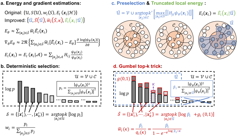
Figure 1: (a) The entire VMC workflow can be broadly divided into four components: (1) the total space $\mathcal{U}$, where amplitudes are computed at each iteration; (2) the sample $\mathcal{S}(\mathcal{U})$ drawn from $\mathcal{U}$; (3) the importance weights $w_{i}(\mathcal{S})$ assigned to the sampled configurations; and (4) the computation of the local energy $E_{l}(\mathbf{x}|\mathcal{A})$ given a subspace $\mathcal{A}$, where $\mathcal{A}$ denotes the set of configurations considered when iterating over all single and double excitations $\ket{\mathbf{x}_{j}}\in\{D^{SD}_{i}\}$ Examples of $\mathcal{A}$ are the full Hilbert space $\mathcal{H}$ or the preselected subspace $\tilde{\mathcal{U}}$ (see part (c)) With these four components specified, both the energy and its gradient can be approximated and subsequently used to update the model parameters. (b) Workflow of fixed-size selected configuration (FSSC) [34]. The total space is the union of the core and connected spaces, i.e., $\mathcal{U}=\mathcal{V}\cup\mathcal{C}$. The sample is deterministically constructed by selecting the $k$ unique configurations with the largest amplitude magnitudes, and the importance weights are probabilities renormalized with respect to this sample. The local energy is computed exactly. (c) In this work, we preselect the connected space $\mathcal{C}$ via three steps represented by the three circles. First we identify all connections (via $H$) between core configurations $\ket{\mathbf{x}_{i}}\in\mathcal{V}$ and connected configurations $\ket{\mathbf{x}_{j}}\in\mathcal{C}$ and compute their strength $H_{ji}\psi_{\theta}(\mathbf{x}_{i})$ represented by weighted edges. Then (second circle) only the edge with largest weight is kept for each configuration $\ket{\mathbf{x}_{j}}$. Finally (third circle) the configurations $\ket{\mathbf{x}_{j}}$ with the largest $k^{\prime}$ values as well as all of $\mathcal{V}$ make up the pre-selected subspace $\tilde{\mathcal{U}}$. Amplitudes for this restricted subspace $\tilde{\mathcal{U}}$ are computed to define new probabilities $\tilde{p}_{i}$, which are used for sampling and streamlining local energy calculations via lookup: $\tilde{E}_{l}(\mathbf{x}_{i}|\tilde{\mathcal{U}})$. (d) The sample $\tilde{\mathcal{S}}$ is stochastically generated using the Gumbel top-$k$ trick. By perturbing the log-probabilities $\tilde{p}_{i}$ with Gumbel noise $g_{i}\overset{i.i.d.}{\sim}\text{Gumbel}(0,1)\quad\text{with pdf}\quad f(x)=e^{-(x+e^{-x})}$ the top-$k$ configurations with the largest perturbed log-probabilities are selected to form the sample $\tilde{\mathcal{S}}$. The associated weights $\tilde{w}_{i}(\kappa)$ provide unbiased estimates over $\tilde{\mathcal{U}}$, yielding improved approximations for the full Hilbert space.

II.1 Overview

For a many-body system containing $N_{e}$ electrons and $N_{o}(>N_{e})$ spin-orbitals $\mathcal{B}=\{\phi_{i}\}_{i=1}^{N_{o}}$, the many-electron wavefunction can be expressed in second quantization as $\ket{\psi}=\sum_{i}\psi(\mathbf{x}_{i})\ket{\mathbf{x}_{i}}$ where $\ket{\mathbf{x}_{i}}=\ket{x_{i}^{1\uparrow},\dots,x_{i}^{N_{o}\uparrow},x_{i}^{1\downarrow},\dots,x_{i}^{N_{o}\downarrow}}$ is the i-th computational basis vector, with $x_{i}^{j\uparrow/\downarrow}\in\{0,1\}$ denoting the occupation of the j-th spin-orbital. NQS offer a promising framework for efficiently representing many-electron wavefunctions via machine learning architectures: $\ket{\psi_{\theta}}=\sum_{i}\psi_{\theta}(\mathbf{x}_{i})\ket{\mathbf{x}_{i}}$ where $\theta$ is model parameter. Among various NQS architectures, NNBF has demonstrated strong performance in fermionic systems [23, 24, 22, 34]. The NNBF wavefunction is defined as $\psi_{\theta}(\mathbf{x}_{i})=\sum_{m=1}^{D}\det[\Phi^{m}_{j=\{l|x_{i}^{l}=1\},k}(\mathbf{x}_{i};\theta)]$ where $\Phi^{m}_{jk}$ are ”configuration-dependent” single-particle orbitals (SPOs) output by NNBF’s internal network.

To determine the ground state of quantum systems, rather than solving the electronic Schrödinger equation directly, VMC reformulates it as an optimization problem by minimizing the variational energy

$$E_{\theta}=\frac{\bra{\psi_{\theta}}\hat{H}\ket{\psi_{\theta}}}{\innerproduct{\psi_{\theta}}{\psi_{\theta}}}=\mathbb{E}\left[E_{l}(\mathbf{x})\right]$$ (1)

where $\mathbb{E}[\cdot]=\mathbb{E}_{p_{\theta}(\mathbf{x})}[\cdot]$ for brevity, and the local energy is $E_{l}(\mathbf{x})=\frac{\bra{\psi_{\theta}}\hat{H}\ket{\mathbf{x}}}{\bra{\psi_{\theta}}\ket{\mathbf{x}}}$, with the quantum chemical Hamiltonian taking the form

$$\hat{H}=\sum_{i,j,\sigma}t_{ij}\hat{c}_{i,\sigma}^{\dagger}\hat{c}_{j,\sigma}+\frac{1}{2}\sum_{i,j,k,l,\sigma,\sigma^{\prime}}V_{ijkl}\hat{c}_{i,\sigma}^{\dagger}\hat{c}_{j,\sigma^{\prime}}^{\dagger}\hat{c}_{l,\sigma^{\prime}}\hat{c}_{k,\sigma}.$$ (2)

. The gradient of energy is then given by

$$\nabla_{\theta}E_{\theta}=2\Re{\mathbb{E}\left[\frac{\partial\ln{\absolutevalue{\psi_{\theta}(\mathbf{x})}}}{\partial\theta}\left[E_{l}(\mathbf{x})-E_{\theta}\right]\right]}$$ (3)

, which allows iterative updates of $\theta$ using gradient descent or more advanced optimization techniques.

For molecular Hamiltonians, previous studies [27, 34] have shown that estimating equation (1) and (3) using conventional MCMC methods, such as the Metropolis–Hastings algorithm, is inefficient. This inefficiency stems from pronounced peaks around the Hartree–Fock (HF) state and nearby excited states [39, 40], which lead to excessive resampling of dominant configurations and thus waste computational resources. Another computational challenge related to the molecular Hamiltonian is that the local energy calculation involves a number of terms that grows quartically with the number of orbitals, causing the computation to become increasingly burdensome as the system size grows.

To mitigate the inefficient sampling issue, several techniques have been developed. Autoregressive neural quantum states, combined with improved sampling methods, enable exact sampling from the Born distribution. Alternatively, approaches inspired by SCI bypass stochastic sampling altogether by deterministically identifying important states and approximating their relative contributions during energy evaluation [30, 34, 35].

In this work, we build on the latter approach. For each optimization step, we start from a core space $\mathcal{V}$ containing a fixed set of unique, important configurations. We then introduce a method to construct a larger important subspace $\tilde{\mathcal{U}}$. From this larger subspace, we generate a more efficient approximation of the local energy $\tilde{E}_{l}(\mathbf{x}|\tilde{\mathcal{U}})$. Additionally, we develop an improved strategy for sampling configurations $\tilde{\mathcal{S}}$ and assigning importance weights $\tilde{w}$, resulting in more accurate estimates of equation (1) and (3). We also generate a new core space for the next optimization step. These are the critical steps required to improve the accuracy and efficiency of the optimization.

II.2 Preselection

In this subsection, we outline our method for generating a compact yet dominant subspace $\tilde{\mathcal{U}}$, which preselects important configurations used throughout the algorithm.

We define the connected space $\mathcal{C}$ as the set of all other configurations connected to the core space $\mathcal{V}$ via non-zero Hamiltonian elements. With a fixed core space size, $\mathcal{C}$ grows quartically with system size. Importantly, identifying configurations in $\mathcal{C}$ does not require amplitude evaluations.

Each connected configuration $\ket{\mathbf{x}_{j}}$ can be linked to multiple core configurations $\ket{\mathbf{x}_{i}}$, with connection strengths quantified by $\psi_{\theta}(\mathbf{x}_{i})H_{ij}$ where “strength” can be realized either through strong Hamiltonian connections ($H_{ij}$ large) or proximity to dominant configurations ($\psi_{\theta}(\mathbf{x}_{i})$ large). The strongest of these connections is then defined as the importance score for element $x_{j}$:

$$I(\mathbf{x}_{j})=\underset{\ket{\mathbf{x}_{i}}\in\mathcal{V}}{max}\absolutevalue{\psi_{\theta}(\mathbf{x}_{i})H_{ij}}.$$ (4)

This metric closely parallels the heuristic used in Heat-bath Configuration Interaction (HCI) [9] for determinant selection: $f_{HCI}(\mathbf{x_{j}})=\underset{i\in\{D^{core}\}}{max}(\absolutevalue{H_{ji}c_{i}})$, which approximates the first-order perturbative correction $\absolutevalue{\frac{\sum_{i}H_{ji}c_{i}}{E_{0}-H_{jj}}}$.

To construct the pre-selected space $\tilde{\mathcal{U}}$, we retain the entire core space and select a fraction, set to $1/(N_{o}-N_{e})$ in this work, of $\mathcal{C}$ with the largest importance score:

$$\tilde{\mathcal{U}}=\mathcal{V}\cup\underset{\ket{\mathbf{x}_{j}}\in\mathcal{C}}{\text{argtop}k^{\prime}}[\underset{\ket{\mathbf{x}_{i}}\in\mathcal{V}}{\text{max}}|H_{ji}\psi_{\theta}(\mathbf{x}_{i})|]$$ (5)

where $k^{\prime}=\absolutevalue{\mathcal{C}}/(N_{o}-N_{e})$. We define the probability distribution:

$$\tilde{p}_{i}=\frac{\psi^{2}_{\theta}(\mathbf{x}_{i})}{\sum_{\ket{\mathbf{x}_{j}}\in\tilde{\mathcal{U}}}\psi^{2}_{\theta}(\mathbf{x}_{j})}\quad\forall\ket{\mathbf{x}_{i}}\in\tilde{\mathcal{U}},$$ (6)

Notice that only amplitudes in $\tilde{\mathcal{U}}$ need to be computed and these amplitudes are stored for the rest of the optimization step, preventing resource waste on insignificant configurations.

We can better understand why these preselected configurations are a reasonable choice by recognizing that the connected space $\mathcal{C}$ naturally emerges during the local energy evaluation with respect to the core space $\mathcal{V}$:

$$E_{\theta}\approx\frac{1}{\sum_{\ket{\mathbf{x}_{k}}\in\mathcal{V}}\psi^{2}_{\theta}(\mathbf{x}_{k})}\sum_{\ket{\mathbf{x}_{i}}\in\mathcal{V},\ket{\mathbf{x}_{j}}}\psi_{\theta}(\mathbf{x}_{i})H_{ij}\psi_{\theta}(\mathbf{x}_{j}).$$ (7)

This expression shows that each connected configuration $\ket{\mathbf{x}_{j}}$ may appear multiple times through different connections, contributing to the energy via terms weighted by $\psi_{\theta}(\mathbf{x}_{i})H_{ij}$. This observation highlights that computing $\psi_{\theta}(\mathbf{x}_{j})$ is only meaningful if at least one of these connection weighs is non-negligible. The importance score in equation (4) captures this idea by selecting the strongest connection for each $\ket{\mathbf{x}_{j}}$, ensuring that configurations with negligible contributions are excluded from the preselected space.

II.3 Streamlined local energy calculations

In this subsection, we propose a strategy, building on Section II.2, to accelerate the calculation of the local energy—identified as one of the primary computational bottlenecks in NQS-based quantum chemistry. Computing $E_{l}(\mathbf{x}_{i})=\sum_{\ket{\mathbf{x}_{j}}}H_{ij}\frac{\psi(\mathbf{x}_{i})}{\psi(\mathbf{x}_{j})}$ requires evaluating ansatz amplitudes for all $\ket{\mathbf{x}_{j}}$ connected to $\ket{\mathbf{x}_{i}}$ through nonzero $H_{ij}$. For second-quantized molecular Hamiltonians, the number of such terms grows quartically with system size, making this step computationally expensive.

To mitigate this cost, we introduce a truncated approximation of the local energy by leveraging the preselected important subspace $\tilde{\mathcal{U}}$ from Section II.2:

$$\tilde{E}_{l}(\mathbf{x}_{i})=E_{l}(\mathbf{x}_{i}|\tilde{\mathcal{U}})=\sum_{\ket{\mathbf{x}_{j}}\in\tilde{\mathcal{U}}}H_{ij}\frac{\psi(\mathbf{x}_{j})}{\psi(\mathbf{x}_{i})}.$$ (8)

Because the amplitudes for configurations in $\tilde{\mathcal{U}}$ are already precomputed, the evaluation of this truncated local energy avoids repeated, costly wavefunction evaluations. Storing $\tilde{\mathcal{U}}$ in lexicographical order further enables efficient amplitude retrieval through $O(\log(\absolutevalue{\tilde{\mathcal{U}}}))$ lookups.

Our approach for computing the local energy shares conceptual similarities with other recent methods [30, 32, 35, 36], where the local energy sum is restricted to the sample set $\mathcal{S}$ generated by their sampling schemes. However, a key distinction is that $\tilde{\mathcal{U}}$ in our method is both larger than $\mathcal{S}$ and prefiltered for importance. This ensures that the truncated sum retains significant contributions to the local energy while providing a more accurate approximation with comparable or even reduced computational cost.

II.4 Gumbel top-k trick

In this section, we introduce a new sampling method that provides better approximations of the energy and its gradients than the estimates given by the fixed-size selected configuration (FSSC) scheme [34], while maintaining the same time complexity. Although Ref. 34 has shown that, for a given batch size, the FSSC scheme outperforms the MCMC scheme by capturing the most significant distinct configurations and avoiding sequential, redundant stochastic sampling, there is still room for improvement.

A key observation is that borderline configurations—those whose amplitude magnitudes are just below the smallest amplitude in the selected sample—may contribute nontrivially to the energy and gradient evaluations. As optimization progresses, a small batch size combined with the deterministic nature of the FSSC scheme may prevent these borderline configurations from being selected, potentially introducing bias. To investigate this, we perform a simple test on the Li₂O molecule in the STO-3G basis set comparing the FSSC and standard MCMC schemes. As shown in Fig. 2, the MCMC scheme achieves a lower variational energy with fewer unique configurations, even though it requires a larger total batch size and therefore is slower. This observation on one hand reinforces the inefficiency of standard MCMC sampling for second-quantized molecular simulations, while on the other hand suggesting that stochastic estimation—when paired with an optimization method leveraging the entire optimization history for parameter updates—could possibly yield estimates that are less biased than purely deterministic methods with the same number of unique samples.

This finding motivates us to enhance the FSSC scheme by incorporating stochasticity while preserving its unique sample selection feature, i.e., sampling without replacement (SWOR). To achieve this, we employ the Gumbel top-$k$ trick [41, 42], a powerful SWOR technique that extends the Gumbel-max trick. By adding independently sampled Gumbel noise to the (unnormalized) log-probabilities of categories and selecting the top-$k$ perturbed values, one can sample from the categorical distribution without replacement. Importantly, Gumbel noise sampling is highly parallelizable, making it suitable for efficient GPU implementation, and it yields unbiased estimates when properly weighted [42, 41].

A natural candidate for applying the Gumbel top-$k$ trick is the preselected subspace $\tilde{\mathcal{U}}$ from Section II.2. Unlike the original FSSC scheme, which relies on the dominance of the core space $\mathcal{V}$, using the Gumbel top-$k$ trick allows us to unbiasedly represent $\tilde{\mathcal{U}}$, which is more representative than $\mathcal{V}$ alone, as it is preselected for importance and grows extensively with system size when $\absolutevalue{\mathcal{V}}$ is fixed. By introducing Gumbel noise, previously excluded borderline configurations can be sampled, improving the approximation of both energy and gradients. Moreover, the computational overhead is minimal since Gumbel noise generation is inexpensive.

To formalize this approach, we describe how the Gumbel top-$k$ trick is used to form the sample $\tilde{\mathcal{S}}$ and assign importance weights $\tilde{w}_{i}$ for constructing more unbiased estimates of equation (1) and (3). The new core space can still be deterministically selected as in Ref. 34 or simply chosen as $\tilde{\mathcal{S}}$. Samples are drawn from $\tilde{\mathcal{U}}$ by perturbing the log probability [Eq. (6)] with independently and identically distributed Gumbel noise:

$$g_{i}\overset{i.i.d.}{\sim}\text{Gumbel}(0,1)\quad\text{with pdf}\quad f(x)=e^{-(x+e^{-x})},$$ (9)

and selecting the top-$k$ configurations with perturbed log-probabilities:

$$\tilde{\mathcal{S}}=\underset{\ket{\mathbf{x}_{i}}\in\tilde{\mathcal{U}}}{\text{argtop}k},[G_{i}=\log\tilde{p}_{i}+g_{i}].$$ (10)

The corresponding importance weight is then given as:

$$\tilde{w}_{i}(\kappa)=\frac{\tilde{p}_{i}}{q_{i}(\kappa)}=\frac{\tilde{p}_{i}}{1-e^{-e^{\log\tilde{p}_{i}-\kappa}}},$$ (11)

where $\kappa$ is the $(k+1)$-th largest $G_{i}$, serving as the empirical threshold (since $\ket{\mathbf{x}_{i}}\in\tilde{\mathcal{S}}$ if $G_{i}>\kappa$), and $q_{i}(\kappa)=P(G_{i}>\kappa)$ denotes the inclusion probability of selecting sample $i$. Importance weights are typically renormalized to reduce variance in practice [42], albeit at the cost of introducing bias.

Using these weights and the Gumbel-top-$k$-selected samples $\tilde{\mathcal{S}}$, we construct improved estimates for the energy and gradient:

$$E_{\theta}\approx\sum_{\ket{\mathbf{x}_{i}}\in\tilde{\mathcal{S}}}\tilde{w}_{i}(\kappa)\tilde{E}_{l}(\mathbf{x}_{i}|\tilde{\mathcal{U}})$$ (12)

and

$$\nabla_{\theta}E_{\theta}\approx 2\Re{\sum_{\ket{\mathbf{x}_{i}}\in\tilde{\mathcal{S}}}\tilde{w}_{i}(\kappa)\left[\tilde{E}_{l}(\mathbf{x}_{i}|\tilde{\mathcal{U}})-E_{\theta}\right]\frac{\partial\ln{\absolutevalue{\psi_{\theta}(\mathbf{x}_{i})}}}{\partial\theta}}.$$ (13)

where $\tilde{E}_{l}(\mathbf{x}_{i}|\tilde{\mathcal{U}})$ is equation (8). While equation (12) and (13) are not fully unbiased estimators of equation (1) and (3), they significantly reduce bias compared to the deterministic FSSC approach.

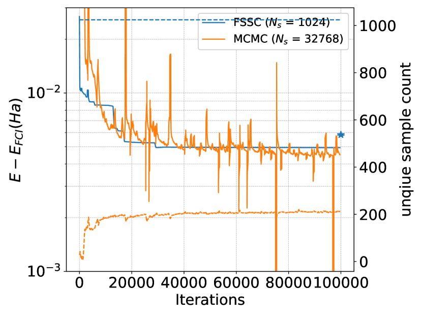
Figure 2: Comparison of the energy optimization curve and the number of unique configurations sampled per iteration between the FSSC ($N_{s}=1024$) and MCMC ($N_{s}=32768$) schemes for Li₂O, using the STO-3G basis set and canonical HF orbitals. Solid lines represent the objective energy optimization curve, while dashed lines indicate the number of unique configurations sampled per iteration. The blue star marks the post-training MCMC inference energy for the FSSC scheme. A moving average window of 400 is applied for improved readability.

II.5 Encode physical knowledge

II.5.1 Enforce Spin-flip symmetry

In this work, we propose a general approach to enforce the spin-flip symmetry on top of the NNBF ansatz. We define the spin-flip operator $\hat{F}$ as a transformation that exchanges the spin components of a configuration: $\hat{F}:\ket{x_{i}^{1\uparrow},\cdots,x_{i}^{N_{o}\uparrow},x_{i}^{1\downarrow},\cdots,x_{i}^{N_{o}\downarrow}}\mapsto\ket{x_{i}^{1\downarrow},\cdots,x_{i}^{N_{o}\downarrow},x_{i}^{1\uparrow},\cdots,x_{i}^{N_{o}\uparrow}}$. For eigenstates $\ket{\psi}$ with total spin zero, this symmetry implies $\hat{F}\ket{\psi}=\pm\ket{\psi}$, and thus the amplitudes of spin-flip-equivalent configurations, $\ket{\mathbf{x}_{i}}$ and $\ket{\hat{F}\mathbf{x}_{i}}$, satisfy $\psi(\hat{F}\mathbf{x}_{i})=\pm\psi(\mathbf{x}_{i})$. This condition holds in second-quantized molecular systems where spin orbitals are constructed with spin-independent spatial components, as in restricted HF methods.

We impose this symmetry by defining the spin-flip-symmetric wavefunction as:

$$\psi_{SFS,\theta}(\mathbf{x})=\psi_{\theta}(\mathbf{x})\pm\psi_{\theta}(\hat{F}\mathbf{x}).$$ (14)

This construction ensures both $\hat{F}\ket{\psi_{SFS,\theta}}=\pm\ket{\psi_{SFS,\theta}}$ and $\psi_{SFS,\theta}(\hat{F}\mathbf{x})=\pm\psi_{SFS,\theta}(\mathbf{x})$. Unlike the approach in Ref. [28], which enforces a weaker form of the symmetry ($\absolutevalue{\psi(\hat{F}\mathbf{x}_{i})}=\absolutevalue{\psi(\mathbf{x}_{i})}$) through specialized preprocessing of subnetwork inputs and postprocessing of outputs, our method is more general. It requires only the addition of a single equation atop any wavefunction ansatz, ensuring full spin-flip symmetry while naturally preserving the relative sign consistency between spin-flip-equivalent configurations.

II.5.2 Spin-flip-symmetry-aware strategies

When a wavefunction ansatz is constructed as in Section II.5.1, several strategies can be leveraged to enhance the training pipeline.

For constructing the preselected subspace $\tilde{\mathcal{U}}$, among each pair of spin-flip-equivalent configurations (or the single representative in the spin-flip-symmetric case), only the one with the higher importance score should be retained, as both share identical amplitude magnitudes.

During sample generation via the Gumbel top-$k$ trick, non-spin-flip-symmetric configurations $\ket{\mathbf{x}_{i}}$ have the same probability and local observables (e.g., local energy) as their excluded counterparts $\hat{F}\ket{\mathbf{x}_{i}}$. This redundancy can be utilized by doubling the probability of non-symmetric configurations:

$$\tilde{p}_{\text{SFS},i}=\begin{cases}2\tilde{p}_{i},&\text{if }\ket{\mathbf{x}_{i}}\text{ is non-spin-flip-symmetric},\\ \tilde{p}_{i},&\text{if }\ket{\mathbf{x}_{i}}\text{ is spin-flip-symmetric}.\end{cases}$$ (15)

Similarly, when evaluating the truncated local energy [Eq. (8)], the lookup for the precomputed amplitude $\psi_{\theta}(\mathbf{x}_{j})$ in $\tilde{\mathcal{U}}$ should also include $\psi_{\theta}(\hat{F}\mathbf{x}_{j})$.

These modifications effectively double the sample size without compromising the efficiency of the truncated local energy strategy, as spin-flip-symmetric configurations are significantly fewer compared to their non-symmetric counterparts.

II.5.3 Orbital occupation

We introduce a trainable discrete orbital envelope designed to capture general occupation patterns of molecular orbitals. In quantum chemistry, it is well established that lower-energy orbitals have higher occupation probabilities, with core electrons typically occupying the lowest-energy orbitals. Consequently, configurations further from the HF reference generally have lower probabilities.

To incorporate this prior knowledge, we define an ordered position representation of the configuration bitstring as $\mathbf{y}(\mathbf{x})=vector(\{i|x^{i}=1\})$, which lists the indices of occupied orbitals in ascending order. Using this representation, we propose the following trainable discrete orbital envelope:

$$\pi_{\mathbf{\alpha}}(\mathbf{y}(\mathbf{x}))=$$,

where $\alpha$ is a set of trainable parameters. Each term acts as a penalty based on the displacement of the occupied orbital from its reference position, with lower-indexed orbitals favored for lower-indexed electrons. To respect spin-flip symmetry, both spin channels share the same set of envelope parameters $\alpha$. See Appendix B for a visualization and analysis of the learned orbital envelope parameters after training.

II.5.4 Selection of orbitals

In the framework of SCI, the choice of single-particle orbitals (molecular orbitals) significantly affects the compactness of the wavefunction and, consequently, the convergence of the simulation with respect to the number of determinants. Selecting orbitals that achieve a given accuracy with the fewest configurations is therefore crucial.

A common choice is the set of natural orbitals [43], defined as the eigenstates of the 1-RDM derived from other wavefunctions, such as those from HF, MP2, CISD, or CCSD. Expansions based on natural orbitals generally converge more rapidly than those using canonical HF orbitals.

For all-electron calculations, the selection of single-particle orbitals does not influence the exact ground-state energy. Hence, unless otherwise specified, we use CCSD natural orbitals in all-electron calculations to promote faster convergence.

III Results

We evaluate the performance of NNBF combined with the algorithmic enhancements proposed in Section II.2, II.3, II.4, and II.5 on various molecules using the STO-3G basis set as well as on a paradigmatic strongly correlated system: frozen-core N₂ with the cc-pVDZ basis set. To demonstrate the improvements from these enhancements, we compare results with our previous algorithm [34] and conduct a thorough ablation study by cumulatively adding the proposed techniques. We also investigate the relationship between NNBF’s representability and the inverse participation ratio (IPR). Details on the default network architectures, hyperparameters, training routine, and post-training MCMC inference procedure are provided in Appendix A.

III.1 Benchmarks

We assess the performance of our algorithms by first comparing molecular ground-state energies with CCSD and CCSD(T) baselines and other NQS results, using molecular geometries sourced from PubChem [44]. All calculations follow the protocols described in Sections II.2, II.3, II.4, and II.5, with a fixed batch size $N_{s}=1024$, which is equal to the core space size ($\absolutevalue{\mathcal{V}}$). Table 1 shows that NNBF, using only default hyperparameters and the improved algorithms, not only outperforms conventional CCSD methods but also achieves lower energies than all existing NQS approaches, particularly excelling in larger molecular systems. For smaller molecules where FCI energies exist, it’s often the case that NNBF is closer than CCSD(T) to the exact answer. In our largest two molecules, there is no FCI energy to compare against. In these cases, we find the energy is very close to CCSD(T); because CCSD(T) isn’t variational, it is unclear in those cases whether NNBF or CCSD(T) is better.

To further benchmark our method, we calculate the ground-state energy of frozen-core N₂ using the cc-pVDZ basis. As shown in Table 2, with canonical HF orbitals, NNBF achieves superior variational energies compared to SCHI [10] and ASCI [12], which represent the state of the art in SCI methods for QC. After orthonormally rotating the unfrozen orbitals—an operation that does not affect the ground-state calculation for either frozen-core or all-electron treatments—NNBF attains variational energies that are lower but still within error bars (approximately 0.1 mHa difference) of the best results from SCHI, ASCI, and FCIQMC [38], underscoring its ability to capture strongly correlated systems. Other NQS methods [35] yield energy differences on the order of several mHa, further highlighting the superiority of the NNBF ansatz. These results are obtained using a moderate batch size ($N_{s}=8192$) and a neural network with $h=512$ hidden units.

To demonstrate the impact of our algorithmic improvements, we compare the current algorithm with that of Ref. 34 by studying how the batch size used during optimization affects NNBF performance on Li₂O with the STO-3G basis set and canonical HF orbitals. Figure 3 shows that while both methods exhibit polynomial scaling of energy improvement with batch size, our updated algorithm achieves a faster convergence rate of $O(N_{s}^{-1.979616\pm 0.006350})$ compared to $O(N_{s}^{-1.166309\pm 0.014370})$ for the previous method. Notably, our new approach requires orders of magnitude fewer samples to reach the same energy accuracy. Furthermore, the wall time per optimization step is significantly reduced—details are discussed in Section III.2.

Molecule	$N_{t}$	CCSD	CCSD(T)	FCI	Best NQS	NNBF
N2	$1.44\times 10^{4}$	-107.656080	-107.657850	-107.660206	-107.6602[31]	-107.660218(67)
CH4	$1.59\times 10^{4}$	-39.806022	-39.806164	-39.806259	-39.8062[31]	-39.806258(22)
LiF	$4.41\times 10^{4}$	-105.159235	-105.166274	-105.166172	-105.1661[31]	-105.166169(18)
CH2O	$2.45\times 10^{5}$	112.498566	-112.500465	-112.501253	-112.500944[29]	-112.501199(22)
LiCl	$1.00\times 10^{6}$	-460.847579	-460.849980	-460.849618	-460.8496[28]	-460.849614(10)
CH4O	$4.01\times 10^{6}$	-113.665485	-113.666214	-113.666485	-113.665485[29]	-113.666379(76)
Li2O	$4.14\times 10^{7}$	-87.885514	-87.893089	-87.892693	-87.8922[31]	-87.892689(25)
C2H4O	$2.54\times 10^{9}$	-151.120474	-151.122748	-	-151.12153[31]	-151.122602(39)
C2H4O2	$5.41\times 10^{11}$	-225.050896	-225.057823	-	-225.0429767[29]	-225.055531(75)

Table 1: Benchmarking NNBF ground-state energies against conventional CCSD, CCSD(T), and FCI results, as well as the best published NQS results, with footnotes indicating the respective methods (excluding our previous work [34]). $N_{t}$ represents the total number of physically valid configurations that conserve both particle number and total charge. For NNBF, we run three different training runs each following the default settings specified in Appendix A with $N_{s}=1024$, and the NNBF energy column reports the best post-training MCMC inference energy.

Method	Number of determinants	Variational energy	Total energy
HF orbitals
SHCI[10]	37593	-109.2692	-109.2769
ASCI[12]	10000	-109.26419	-109.27687
ASCI[12]	30000	-109.26936	-109.27691
ASCI[12]	100000	-109.27335	-109.27698
FCIQMC[38]	-	-	-109.2767(1)
NNBF	8192	-109.27616(5)	-
MP2 natural orbitals
NNBF	8192	-109.2771(1)	-
Dynamic orbital rotations
ASCI[12]	10000	-109.26837	-109.27708
ASCI[12]	100000	-109.27522	-109.27699
ASCI[12]	300000	-109.27638	-109.27699

Table 2: Benchmarking the ground-state NNBF energy for the frozen-core calculation of the N₂ molecule at a bond length of 1.0977 $\mathring{A}$, using the cc-pVDZ basis set and canonical Hartree-Fock orbitals. Results are compared with HCI [10], ASCI [12], and FCIQMC[38]. The variational energies of HCI and ASCI are obtained by exact diagonalization of the variational space, with a size equal to the number of determinants, and include second-order perturbative corrections in the total energies. Since the FCIQMC energy is not variational, it is considered the total energy of the method. For NNBF, the number of determinants corresponds to $N_{s}$ used in our improved algorithm for the NNBF ansatz ($h=512$), and its variational energy is obtained from post-training MCMC inference.

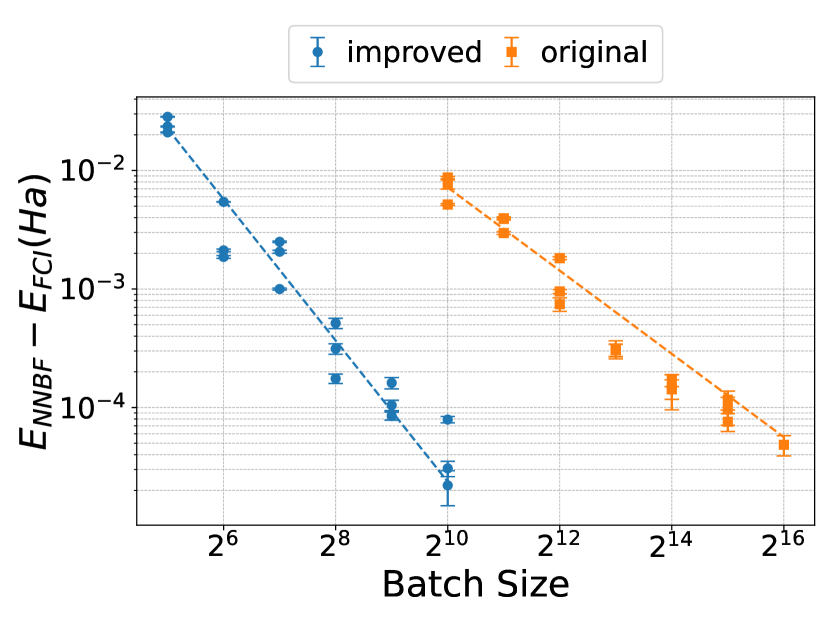
Figure 3: Experiments comparing the impact of batch size $N_{s}$ on energy improvements for Li₂O, using the STO-3G basis set with canonical HF orbitals. Results are shown for the original algorithm from our previous work [34] and our current improved algorithm. The energy error decreases approximately following $O(N_{s}^{-1.979616\pm 0.006350})$ with $R^{2}=0.935316$ for the improved algorithm introduced in this work and $O(N_{s}^{-1.166309\pm 0.014370)})$ with $R^{2}=0.880579$ for the algorithm used in Ref. 34. Here the linear regression is done by the weighted least square method since the reported energies have uncertainties.

III.2 Ablation study

Here we demonstrate how each algorithm introduced in Sections II.2, II.3, II.4, and II.5 improves the energy accuracy and computational efficiency through an ablation study on Li₂O with the STO-3G basis set and HF orbitals. We cumulatively add these enhancements to our previous algorithm [34] to highlight their individual and combined contributions (see Figure 4).

Figure 4 shows that the introduction of the Gumbel top-$k$ trick alone reduces the energy error by two orders of magnitude without additional computational cost. In contrast to Ref. 34, which uses the union of the core space $\mathcal{V}$ and the entire connected space $\mathcal{C}$ as the total space $\mathcal{U}$, our preselection step generates a more compact important subspace $\tilde{\mathcal{U}}$ that is $\frac{1}{N_{o}-N_{e}}$ times smaller than $\mathcal{U}$. This reduces the number of amplitude evaluations by the same factor, decreasing the per-optimization-step time from 0.47 to 0.28 seconds.

The truncated local energy evaluation strategy further accelerates training by replacing full neural network evaluations with simpler $O(\log{\absolutevalue{\tilde{\mathcal{U}}}})$ lookups, improving computational efficiency (the per-iteration time is reduced from 0.28 to 0.07 seconds) without compromising energy accuracy.

Finally, incorporating physical knowledge into the model architecture enhances the expressiveness of the NNBF ansatz and further improves energy accuracy, all while maintaining the same computational complexity. Although integrating spin-flip symmetry increases the wall time per optimization step by a factor of 1.42, the scaling remains unchanged.

Altogether, these enhancements enable us to achieve significantly better energy accuracy and considerably reduce computational time for a given batch size and network architecture.

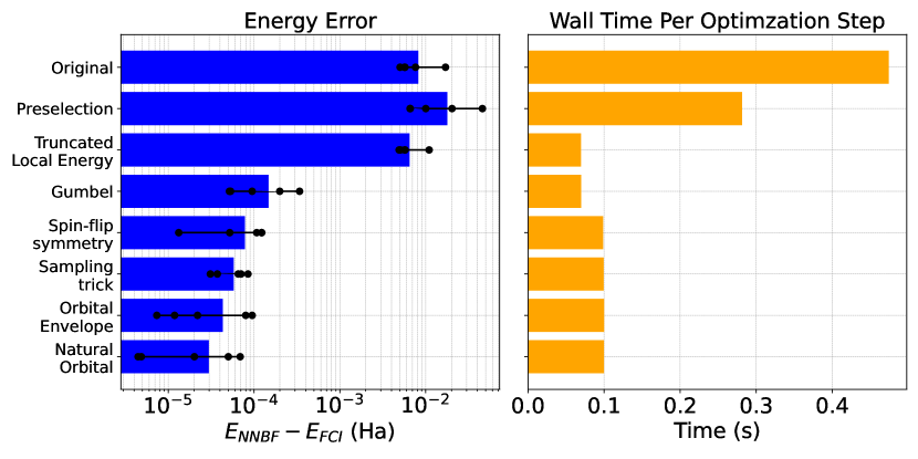
Figure 4: Evaluation of accuracy and speed improvements achieved through the algorithmic enhancements detailed in Section II.4, II.2, II.3, and II.5 for training Li₂O with the STO-3G basis set and canonical HF orbitals. The experiments use a fixed batch size of $N_{s}=1024$. Each bar represents the average energy error and per-iteration wall time across different seeds, with individual points corresponding to separate runs of the same model and method. The algorithmic improvements are applied cumulatively

III.3 NNBF Expressiveness and the Role of IPR

Lastly, we examine the relationship between the inverse participation ratio (IPR) of the quantum state and the expressiveness of NNBF. Similar experiments have been conducted in Ref. 36 using autoregressive neural networks. In our study, we consider N₂ and CH₄ using the STO-3G basis set with HF orbitals, and use a vanilla NNBF ansatz—without employing spin-flip symmetry, spin-flip-symmetry-aware techniques, and orbital envelope features. To eliminate approximation errors in energy and its gradient, training is performed over the entire Hilbert space.

Figure 5 shows that the absolute relative energy error increases as the IPR decreases for both N₂ and CH₄ across both overparameterized ($h=64$) and underparameterized ($h=16$ and $h=32$) cases. While this observation is consistent with the intuition that highly peaked probability distributions are easier to optimize, other factors likely influence overall performance. For example, the complexity of the amplitude landscape, including the distribution of nodal regions and the interplay between electron correlation and orbital symmetries, might also contribute to these effects. Unraveling these factors represents an important direction for future research, and our findings offer valuable insights into the expressiveness of neural quantum states.

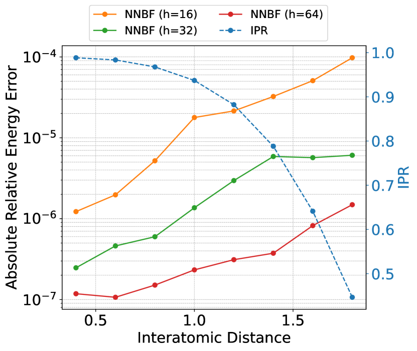
(a) CH₄

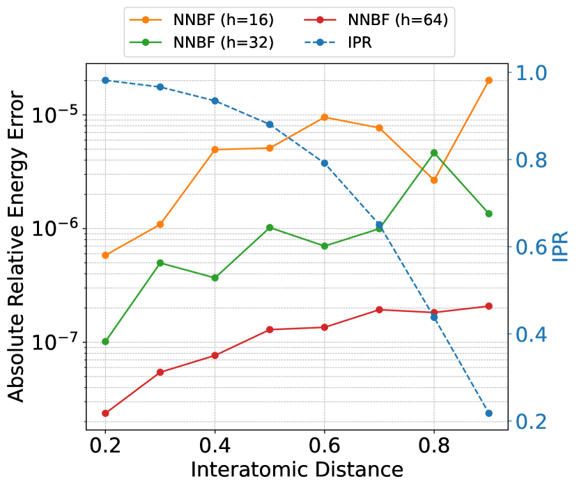
(b) N₂

Figure 5: Investigating the relationship between NNBF expressiveness and the inverse participation ratio (IPR) of the molecular ground state through the dissociation curves of (a) CH₄ and (b) N₂ molecules, using the STO-3G basis set with canonical HF orbitals. For each set of molecule geometry and network architecture, three trials are performed with different random seeds; each data point shows the smallest absolute relative energy error among them. The relative energy error is computed as the difference between the total NNBF energy and the total FCI energy, divided by the electronic FCI energy (excluding the fixed, non-variational nuclear repulsion contribution). The absolute relative energy error (left y-axis) and ground-state IPR (right y-axis) are plotted as functions of interatomic distance. To eliminate approximation errors in energy and its gradient, optimization is performed over the entire Hilbert space ($N_{s}=N_{t}$). Double precision is employed for exact inference energy calculations, as higher precision becomes crucial when the NNBF state closely approximates the true ground state. Different hidden unit sizes are used to illustrate overparameterized ($h=64$) and underparameterized ($h=16,32$) scenarios.

IV Conclusions

In this work, we have demonstrated that the proposed algorithmic enhancements—preselection, truncated local energy evaluation, Gumbel top-$k$ sampling, and physics-informed encoding—significantly improve the performance of the NNBF ansatz across various molecular systems and strongly correlated problems. Our method consistently achieves lower ground-state energies than existing NQS approaches and surpasses conventional CCSD calculations, particularly for larger molecules where traditional methods struggle. When FCI data is available, NNBF often attains results closer to the exact solution than CCSD(T). In the challenging frozen-core N₂ system with the cc-pVDZ basis, NNBF achieves variational energies competitive with or better than state-of-the-art SCI and FCIQMC methods. The ablation study highlights how each enhancement contributes to both improved energy accuracy and reduced computational cost, with the Gumbel top-$k$ trick alone reducing the energy error by two orders of magnitude without additional overhead and the combination of preselection and truncated local energy strategies further reducing the per-iteration time significantly.

A direct comparison with our previous method [34] further emphasizes the efficiency gains achieved through these improvements. While both approaches exhibit polynomial scaling of energy accuracy with batch size, the updated algorithm achieves a notably faster convergence rate and requires orders of magnitude fewer samples to reach the same level of precision. For example, in the Li₂O benchmark, the improved method attains similar accuracy with a batch size hundreds of times smaller than that required by the previous approach. This reduction in sample complexity, combined with decreased wall time per optimization step, underscores the effectiveness of the proposed techniques in enhancing computational efficiency. Lastly, our analysis of NNBF expressiveness shows that lower IPR values generally correspond to higher relative energy errors, indicating that more delocalized states are harder to approximate. Despite this trend, factors beyond IPR also influence the optimization difficulty, highlighting the complexity of the amplitude landscape.

Future work could focus on adopting more advanced optimizers, such as minSR methods [45, 46], leveraging dynamic orbital rotations to produce more compact wavefunctions [47], and integrating spin-flip symmetry directly into the NNBF’s internal neural network structure. We anticipate that the techniques developed in this study will enable more efficient and reliable NQS optimization, expanding the range of practical applications in quantum chemistry.

Appendix A Experimental Setup

The internal neural network used in this work is a multilayer perceptron (MLP) with $h$ hidden units, $L$ hidden layers, and $D$ backflow determinants, where residual connections are incorporated when $L>1$. We use the AdamW optimizer to minimize the energy expectation value of our NNBF ansatz and approximate the ground state of various molecules. The default hyperparameters are listed in Table 3. Baseline energies for HF, CCSD, CCSD(T), and FCI calculations are obtained using the PySCF software package [48]. Each calculation was performed using 1 NVDIA V100 gpu.

After training with the algorithmic enhancements described in Sections II.2, II.3, II.4, and II.5, we perform a separate MCMC inference step to estimate the variational energy of the trained NNBF state. This inference procedure follows the approach detailed in Appendix A of Ref. 34, providing an unbiased stochastic estimate of the energy. These values are reported in all experiments, except when investigating the relationship between NNBF expressiveness and the IPR, where the energy is computed exactly over the full Hilbert space.

Hyperparameter	Value
Energy unit	Hartree
Framework	JAX
Precision	float32
Optimizer	AdamW
AdamW’s $\beta_{1}$	0.9
AdamW’s $\beta_{2}$	0.999
AdamW’s $\epsilon$	$1\times 10^{-8}$
AdamW’s $\lambda$	0.0001
Learning rate	$10^{-3}\times(1+10^{-4}t)^{-1}$
Training iterations	100000
Number of pretraining walkers	8192
Pretraining iterations	500
Number of dominant configurations	8
for walker initialization
MCMC burn-in steps	$20\times 2N_{e}$
right after initialization
Number of MCMC walkers	1024
MCMC downsample interval	$1\times 2N_{e}$
MCMC iterations	1000
Number of hidden layers	2
Hidden units	256
Number of determinants	1
Preselection reduction factor	$1/(N_{o}-N_{e})$

Table 3: Default hyperparameters used for all experiments in the paper, unless explicitly stated otherwise

symbol	description
$N_{e}$	number of electrons
$N_{o}$	number of spin-orbitals
$N_{t}=\binom{N_{o}}{N_{e}}^{2}$	number of physically valid configurations
$N_{s}$	number of samples
$L$	number of hidden layers
$h$	hidden units
$D$	number of determinants
$N_{w}$	number of MCMC walkers

Table 4: Table of notations

Appendix B Learned Orbital Envelope Parameters

This section illustrates what the orbital envelope [Eq. (II.5.3)] learns during training by visualizing the distribution of its trainable parameters for the last four molecules listed in Table 1. All $\alpha$ values are initially set to a small value (0.01) to prevent biasing the ansatz. As shown in Figure 6, after training, the $\alpha$ values associated with inner electrons become noticeably larger than those for outer electrons, reflecting the intuitive physical expectation that inner electrons remain closer to the nucleus in lower-energy orbitals.

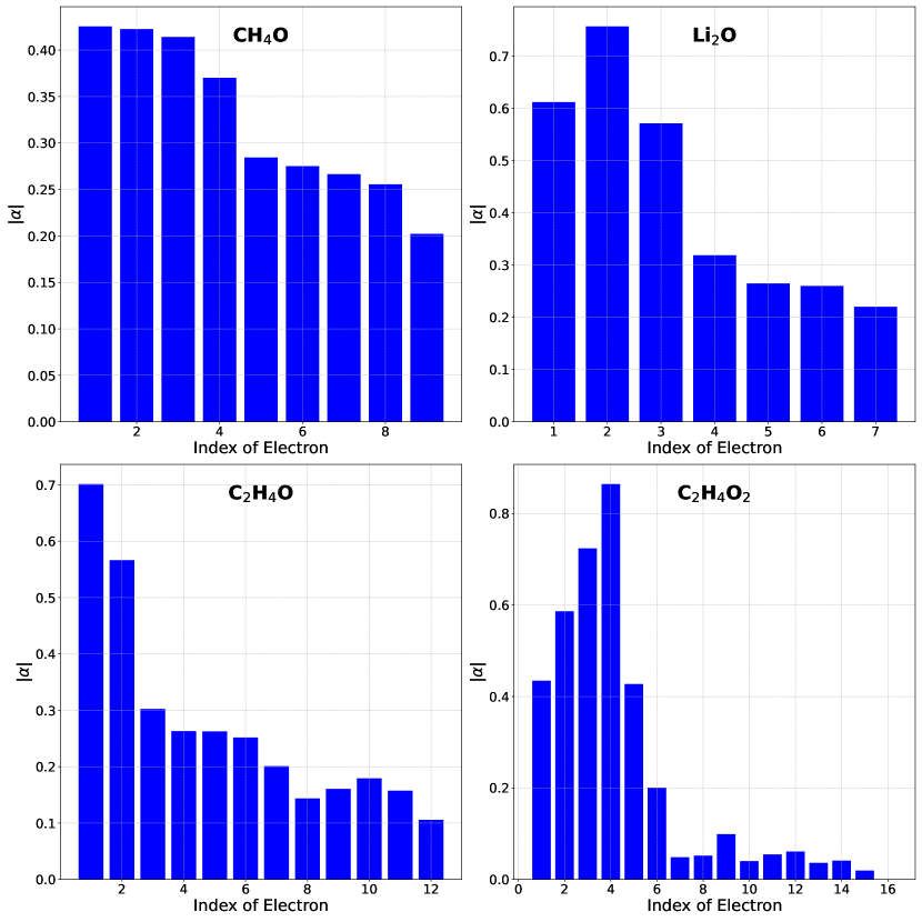
Figure 6: Distribution of the orbital envelope parameters $\alpha_{i}$ after training for CH₄O, Li₂O, C₂H₄O, and C₂H₄O₂ in the STO-3G basis with CCSD natural orbitals. The y-axis shows the absolute value of $\alpha_{i}$, as only its magnitude affects the envelope per Eq. (II.5.3).

References

- Whitfield et al. [2013] J. D. Whitfield, P. J. Love, and A. Aspuru-Guzik, Computational complexity in electronic structure, Phys. Chem. Chem. Phys. 15, 397–411 (2013).
- O’Gorman et al. [2022] B. O’Gorman, S. Irani, J. Whitfield, and B. Fefferman, Intractability of electronic structure in a fixed basis, PRX Quantum 3, 020322 (2022).
- David Sherrill and Schaefer [1999] C. David Sherrill and H. F. Schaefer, The configuration interaction method: Advances in highly correlated approaches, in Advances in Quantum Chemistry (Elsevier, 1999) p. 143–269.
- Coester and Kümmel [1960] F. Coester and H. Kümmel, Short-range correlations in nuclear wave functions, Nuclear Physics 17, 477–485 (1960).
- Foulkes et al. [2001] W. M. C. Foulkes, L. Mitas, R. J. Needs, and G. Rajagopal, Quantum monte carlo simulations of solids, Rev. Mod. Phys. 73, 33 (2001).
- Clark et al. [2011] B. K. Clark, M. A. Morales, J. McMinis, J. Kim, and G. E. Scuseria, Computing the energy of a water molecule using multideterminants: A simple, efficient algorithm, The Journal of Chemical Physics 135, 10.1063/1.3665391 (2011).
- White [1992] S. R. White, Density matrix formulation for quantum renormalization groups, Phys. Rev. Lett. 69, 2863 (1992).
- White and Martin [1999] S. R. White and R. L. Martin, Ab initio quantum chemistry using the density matrix renormalization group, The Journal of Chemical Physics 110, 4127–4130 (1999).
- Holmes et al. [2016] A. A. Holmes, N. M. Tubman, and C. J. Umrigar, Heat-bath configuration interaction: An efficient selected configuration interaction algorithm inspired by heat-bath sampling, Journal of Chemical Theory and Computation 12, 3674–3680 (2016).
- Sharma et al. [2017] S. Sharma, A. A. Holmes, G. Jeanmairet, A. Alavi, and C. J. Umrigar, Semistochastic heat-bath configuration interaction method: Selected configuration interaction with semistochastic perturbation theory, Journal of Chemical Theory and Computation 13, 1595–1604 (2017).
- Tubman et al. [2016] N. M. Tubman, J. Lee, T. Y. Takeshita, M. Head-Gordon, and K. B. Whaley, A deterministic alternative to the full configuration interaction quantum monte carlo method, The Journal of Chemical Physics 145, 10.1063/1.4955109 (2016).
- Tubman et al. [2018] N. M. Tubman, D. S. Levine, D. Hait, M. Head-Gordon, and K. B. Whaley, An efficient deterministic perturbation theory for selected configuration interaction methods (2018).
- Carleo and Troyer [2017] G. Carleo and M. Troyer, Solving the quantum many-body problem with artificial neural networks, Science 355, 602–606 (2017).
- Choo et al. [2019] K. Choo, T. Neupert, and G. Carleo, Two-dimensional frustrated model studied with neural network quantum states, Phys. Rev. B 100, 125124 (2019).
- Choo et al. [2018] K. Choo, G. Carleo, N. Regnault, and T. Neupert, Symmetries and many-body excitations with neural-network quantum states, Phys. Rev. Lett. 121, 167204 (2018).
- Nagy and Savona [2019] A. Nagy and V. Savona, Variational quantum monte carlo method with a neural-network ansatz for open quantum systems, Phys. Rev. Lett. 122, 250501 (2019).
- Sharir et al. [2020] O. Sharir, Y. Levine, N. Wies, G. Carleo, and A. Shashua, Deep autoregressive models for the efficient variational simulation of many-body quantum systems, Phys. Rev. Lett. 124, 020503 (2020).
- Nomura et al. [2017] Y. Nomura, A. S. Darmawan, Y. Yamaji, and M. Imada, Restricted boltzmann machine learning for solving strongly correlated quantum systems, Phys. Rev. B 96, 205152 (2017).
- Ferrari et al. [2019] F. Ferrari, F. Becca, and J. Carrasquilla, Neural gutzwiller-projected variational wave functions, Phys. Rev. B 100, 125131 (2019).
- Stokes et al. [2020] J. Stokes, J. R. Moreno, E. A. Pnevmatikakis, and G. Carleo, Phases of two-dimensional spinless lattice fermions with first-quantized deep neural-network quantum states, Phys. Rev. B 102, 205122 (2020).
- Lin et al. [2023] J. Lin, G. Goldshlager, and L. Lin, Explicitly antisymmetrized neural network layers for variational monte carlo simulation, Journal of Computational Physics 474, 111765 (2023).
- Chen et al. [2022] Z. Chen, D. Luo, K. Hu, and B. K. Clark, Simulating 2+1d lattice quantum electrodynamics at finite density with neural flow wavefunctions (2022).
- Luo and Clark [2019] D. Luo and B. K. Clark, Backflow transformations via neural networks for quantum many-body wave functions, Phys. Rev. Lett. 122, 226401 (2019).
- Liu and Clark [2024a] Z. Liu and B. K. Clark, Unifying view of fermionic neural network quantum states: From neural network backflow to hidden fermion determinant states, Phys. Rev. B 110, 115124 (2024a).
- Pfau et al. [2020] D. Pfau, J. S. Spencer, A. G. D. G. Matthews, and W. M. C. Foulkes, Ab initio solution of the many-electron schrödinger equation with deep neural networks, Physical Review Research 2, 10.1103/physrevresearch.2.033429 (2020).
- Hermann et al. [2020] J. Hermann, Z. Schätzle, and F. Noé, Deep-neural-network solution of the electronic schrödinger equation, Nature Chemistry 12, 891 (2020).
- Choo et al. [2020] K. Choo, A. Mezzacapo, and G. Carleo, Fermionic neural-network states for ab-initio electronic structure, Nature Communications 11, 2368 (2020).
- Barrett et al. [2022] T. D. Barrett, A. Malyshev, and A. I. Lvovsky, Autoregressive neural-network wavefunctions for ab initio quantum chemistry, Nature Machine Intelligence 4, 351 (2022).
- Zhao et al. [2023] T. Zhao, J. Stokes, and S. Veerapaneni, Scalable neural quantum states architecture for quantum chemistry, Machine Learning: Science and Technology 4, 025034 (2023).
- Li et al. [2023] X. Li, J.-C. Huang, G.-Z. Zhang, H.-E. Li, C.-S. Cao, D. Lv, and H.-S. Hu, A nonstochastic optimization algorithm for neural-network quantum states, Journal of Chemical Theory and Computation 19, 8156 (2023).
- Shang et al. [2023] H. Shang, C. Guo, Y. Wu, Z. Li, and J. Yang, Solving schrödinger equation with a language model (2023).
- Wu et al. [2023] Y. Wu, C. Guo, Y. Fan, P. Zhou, and H. Shang, Nnqs-transformer: an efficient and scalable neural network quantum states approach for ab initio quantum chemistry, in Proceedings of the International Conference for High Performance Computing, Networking, Storage and Analysis, SC ’23 (Association for Computing Machinery, New York, NY, USA, 2023).
- Malyshev et al. [2023] A. Malyshev, J. M. Arrazola, and A. I. Lvovsky, Autoregressive neural quantum states with quantum number symmetries (2023).
- Liu and Clark [2024b] A.-J. Liu and B. K. Clark, Neural network backflow for ab initio quantum chemistry, Physical Review B 110, 10.1103/physrevb.110.115137 (2024b).
- Li et al. [2024] X. Li, J.-C. Huang, G.-Z. Zhang, H.-E. Li, Z.-P. Shen, C. Zhao, J. Li, and H.-S. Hu, Improved optimization for the neural-network quantum states and tests on the chromium dimer, The Journal of Chemical Physics 160, 10.1063/5.0214150 (2024).
- Malyshev et al. [2024] A. Malyshev, M. Schmitt, and A. I. Lvovsky, Neural quantum states and peaked molecular wave functions: Curse or blessing? (2024).
- Knitter et al. [2024] O. Knitter, D. Zhao, J. Stokes, M. Ganahl, S. Leichenauer, and S. Veerapaneni, Retentive neural quantum states: Efficient ansätze for ab initio quantum chemistry (2024).
- Cleland et al. [2012] D. Cleland, G. H. Booth, C. Overy, and A. Alavi, Taming the first-row diatomics: A full configuration interaction quantum monte carlo study, Journal of Chemical Theory and Computation 8, 4138–4152 (2012).
- Bytautas and Ruedenberg [2009] L. Bytautas and K. Ruedenberg, A priori identification of configurational deadwood, Chemical Physics 356, 64 (2009), moving Frontiers in Quantum Chemistry:.
- Anderson et al. [2018] J. S. Anderson, F. Heidar-Zadeh, and P. W. Ayers, Breaking the curse of dimension for the electronic schrödinger equation with functional analysis, Computational and Theoretical Chemistry 1142, 66 (2018).
- Vieira [2014] T. Vieira, Gumbel-max trick and weighted reservoir sampling (2014).
- Kool et al. [2019] W. Kool, H. van Hoof, and M. Welling, Stochastic beams and where to find them: The gumbel-top-k trick for sampling sequences without replacement (2019).
- Löwdin [1955] P.-O. Löwdin, Quantum theory of many-particle systems. i. physical interpretations by means of density matrices, natural spin-orbitals, and convergence problems in the method of configurational interaction, Phys. Rev. 97, 1474 (1955).
- Wang et al. [2009] Y. Wang, J. Xiao, T. O. Suzek, J. Zhang, J. Wang, and S. H. Bryant, Pubchem: a public information system for analyzing bioactivities of small molecules, Nucleic Acids Research 37, W623–W633 (2009).
- Chen and Heyl [2024] A. Chen and M. Heyl, Empowering deep neural quantum states through efficient optimization, Nature Physics 20, 1476–1481 (2024).
- Rende et al. [2024] R. Rende, L. L. Viteritti, L. Bardone, F. Becca, and S. Goldt, A simple linear algebra identity to optimize large-scale neural network quantum states, Communications Physics 7, 10.1038/s42005-024-01732-4 (2024).
- Tubman et al. [2020] N. M. Tubman, C. D. Freeman, D. S. Levine, D. Hait, M. Head-Gordon, and K. B. Whaley, Modern approaches to exact diagonalization and selected configuration interaction with the adaptive sampling ci method, Journal of Chemical Theory and Computation 16, 2139–2159 (2020).
- Sun et al. [2017] Q. Sun, T. C. Berkelbach, N. S. Blunt, G. H. Booth, S. Guo, Z. Li, J. Liu, J. D. McClain, E. R. Sayfutyarova, S. Sharma, S. Wouters, and G. K. Chan, Pyscf: the python‐based simulations of chemistry framework, WIREs Computational Molecular Science 8, 10.1002/wcms.1340 (2017).