Comparison of encoding schemes for quantum computing of $S>1/2$ spin chains

Abstract

We compare four different encoding schemes for the quantum computing of spin chains with a spin quantum number $S>1/2$: a compact mapping, a direct (or one-hot) mapping, a Dicke mapping, and a qudit mapping. The three different qubit encoding schemes are assessed by conducting Hamiltonian simulation for $1/2\leq S\leq 5/2$ using a trapped-ion quantum computer. The qudit mapping is tested by running simulations with a simple noise model. The Dicke mapping, in which the spin states are encoded as superpositions of multi-qubit states, is found to be the most efficient because of the small number of terms in the qubit Hamiltonian. We also investigate the $S$-dependence of the time step length $\Delta\tau$ in the Suzuki-Trotter approximation and find that, in order to obtain the same accuracy for all $S$, $\Delta\tau$ should be inversely proportional to $S$.

I Introduction

One of the main applications of quantum computers is the simulation of quantum systems such as molecules [1, 2, 3, 4, 5, 6, 7] and solid-state crystals [2, 8]. While fault tolerance may be required for quantum computers to be truly useful in quantum simulation [9], pioneering calculations using noisy intermediate-scale quantum (NISQ [10]) devices have been carried out for small molecules such as H₂O [11], CH₄[12], C₄H₆ [13], Li₂O [14], and F₂ [15]. However, because of the inherent noise of NISQ devices and because of the deep circuits for the wave function ansatz, the number of qubits in quantum chemistry calculations has been limited to around ten as in the recent calculation of the potential energy curve of F₂ by Guo et al. [15], in which 12 qubits were used.

On the other hand, interacting 1/2-spins on a lattice or in a molecule is a type of quantum system which is well suited for simulation on quantum computers. This is because the two quantum states $|{\uparrow}\rangle$ and $|{\downarrow}\rangle$ of a spin-1/2 site can be straightforwardly mapped to the two qubit states $|0\rangle$ and $|1\rangle$. The simulation of the quantum dynamics of interacting spins can be used to understand the behavior of magnetic materials at low temperatures. The simplest model is the transverse field Ising model [16, 17], which has been a popular model for simulations on quantum computers. Successful demonstrations [18, 19, 20, 21, 22] have been carried out using up to 127 qubits [23]. A slightly more sophisticated model is the Heisenberg model [24, 25, 26], different variants of which have been implemented and simulated on quantum computers [21, 27, 28, 29, 30, 31, 32, 33, 34, 35, 36, 37]. In recent simulations, up to 100 qubits were employed [38, 39].

While the Ising and Heisenberg models usually involve 1/2-spins, systems of interacting spins having a spin quantum number $S>1/2$ are also interesting. Systems of spins with a large $S$ can be realized experimentally in cluster complexes [40, 41, 42], nanomagnets [43, 44, 45, 46], and single-molecule magnets [47, 48, 49, 50, 51, 52]. For example, in [42], a ring-like compound including ten Fe^III ($S=5/2$) and ten Gd^III ($S=7/2$) ions was synthesized. At low temperatures below a few K, the large $S$ spin chains realized in molecules like the one reported in [42] need to be described by a quantum mechanical model of Heisenberg type.

Spin chains with $S>1/2$ are also of theoretical interest for high-spin Kitaev models [53, 54, 55], and in the context of the so-called “Haldane gap” [56, 57, 58, 59, 60], which refers to the finite energy difference between the ground state and the first excited state in the one-dimensional, infinitely long Heisenberg spin chain with integer values of $S$.

Even though most of the previous studies on quantum computing of interacting spin systems have concentrated on $S=1/2$ systems, there exist a few reports on $S=1$ lattices. Quantum annealing has been considered to find the ground state of $S=1$ systems [61]. The real-time dynamics of a single-site $S=1$ system has been simulated using a superconducting qubit quantum computer [62, 63] and that of $S=1$ chains with four [64] and five [65] sites has been simulated using trapped ions (¹⁷¹Yb⁺ [64] and ⁴⁰Ca⁺ [65]).

The number of spin states at each lattice site is $2S+1$, and the total number of spin states for a spin lattice with $N$ sites is equal to $(2S+1)^{N}$, which increases exponentially with increasing $N$. It is in general a difficult task to simulate the spin dynamics of spin lattices using classical computers [66] even though sophisticated Monte Carlo methods [67, 68], density matrix renormalization group methods [69, 70, 71, 72], numerical diagonalization techniques [73, 74, 75], and semiclassical methods [76] have been developed. Therefore, it is worthy to develop simulation algorithms for spin lattices with $S>1/2$ to be executed on quantum computers, because the number of spin states which can be stored in memory in qubit-based quantum computing scales in principle exponentially with the number of qubits.

In the present study, we investigate how spin chain dynamics with arbitrary spin $S$ can be simulated using quantum computers. Because each spin site has $2S+1$ states, which is larger than two when $S>1/2$, more than one qubit must be used for each site. We investigate three kinds of mappings of the spin states to the qubit states, (i) a compact mapping, (ii) a direct mapping, and (iii) a mapping developed for spin-chain simulations using classical computers [67, 68], which we refer to as the Dicke mapping. The Dicke mapping was recently suggested as a suitable mapping for the simulation of $S>1/2$ lattices using neutral atoms [77]. In addition, in view of the recent proposal [65] of using a qudit quantum computer for the simulation of an $S=1$ chain, we also consider (iv) a qudit mapping where each spin-$S$ lattice site is mapped to a qudit having $d=2S+1$ levels. We derive the qubit and qudit Hamiltonians for these different encoding schemes and compare their performances by conducting simulations of a two-site spin model for $S=1$ and $3/2$. The simulations are performed using Quantinuum’s trapped-ion quantum computer H1-1 [78] in the case of the qubit mappings. In the case of the qudit mapping, we conduct the simulations on a classical computer using a completely depolarizing error model to approximately incorporate the effect of the noise. The Dicke mapping is further studied by simulating a four-site spin chain with varying $S$ in the range of $1/2\leq S\leq 5/2$. We also investigate the $S$-dependence of the time step size $\Delta\tau$ in the Suzuki-Trotter approximation.

II Theory

II.1 Hamiltonian and spin states

As the model for spin-spin interaction, we consider the simplest form of the Heisenberg Hamiltonian [25],

$$\mathcal{H} =\frac{J}{\hbar^{2}}\sum_{(m,n)}\hat{\bm{S}}_{m}\cdot\hat{\bm{S}}_{n}$$

$$=\frac{J}{\hbar^{2}}\left(\sum_{(m,n)}\hat{S}_{m}^{z}\hat{S}_{n}^{z}+\frac{1}{2}\sum_{(m,n)}\hat{S}_{m}^{+}\hat{S}_{n}^{-}+\frac{1}{2}\sum_{(m,n)}\hat{S}_{m}^{-}\hat{S}_{n}^{+}\right),$$ (1)

where the sum over $m$ and $n$ is taken over the interacting sites on the lattice, $\hat{\bm{S}}_{n}=(\hat{S}_{n}^{x},\hat{S}_{n}^{y},\hat{S}_{n}^{z})$ is the vector of spin operators acting on site $n$, and $\hat{S}_{n}^{\pm}=\hat{S}_{n}^{x}\pm i\hat{S}_{n}^{y}$. The coupling constant $J$ can be removed by a scaling of the Hamiltonian so that energy is measured in units of $J$ and time in units of $\hbar/J$. The lattice spin states are defined as

$$|\vec{M}\rangle=|M_{N-1},M_{N-2},\ldots,M_{0}\rangle,$$ (2)

where $N$ is the number of sites and $M_{n}$ is the magnetic quantum number of site $n$ taking values of $M_{n}=-S,-S+1,\ldots,S$. The actions of $\hat{S}_{n}^{z}$ and $\hat{S}_{n}^{\pm}$ on the spin state $|M_{n}\rangle$ at a site $n$ are defined as usual as

$$\hat{S}_{n}^{z}|M_{n}\rangle=\hbar M_{n}|M_{n}\rangle$$ (3)

and

$$\qquad\hat{S}_{n}^{\pm}|M_{n}\rangle=\hbar\sqrt{S(S+1)-M_{n}(M_{n}\pm 1)}|M_{n}\pm 1\rangle.$$ (4)

We consider spin lattices where all the sites have the same value of $S$, but the generalization to non-uniform lattices where each site has a different value of $S$ is straightforward.

II.2 Qubit mappings

In order to map the spin states (2) onto qubit or qudit states which can be manipulated on a quantum computer, we consider four different kind of mappings: (i) a compact mapping, (ii) a direct mapping, (iii) a mapping in terms of composite many-qubit states, referred to as the Dicke mapping, and (iv) a qudit mapping.

(i) Compact mapping. In this mapping, which is also referred to as a binary mapping [79], the spin states are mapped to qubit states according to

$$|M\rangle=|{\operatorname{bin}(M+S)}\rangle_{\rm q},$$ (5)

where $\operatorname{bin}(x)$ denotes the binary representation of $x$, and a subscript q is attached to the qubit state to distinguish it from the spin state. The compact mapping requires $K_{\rm q}=\lceil\log_{2}(2S+1)\rceil$ qubits per site, where $\lceil\cdot\rceil$ denotes the ceiling function. For example, for $S=1$, we have three states ($M=-1,$ 0, 1), which are mapped to two-qubit states according to

$$|{-1}\rangle=|{00}\rangle_{\rm q},\text{ }|0\rangle=|{01}\rangle_{\rm q},\text{ }\text{and }|1\rangle=|{10}\rangle_{\rm q}.$$ (6)

The $|{11}\rangle_{\rm q}$ state is not used for $S=1$. To describe a two-site lattice, we need four qubits and use the mapping $|{-1},{-1}\rangle=|{0000}\rangle_{\rm q}$, $|{-1},0\rangle=|{0001}\rangle_{\rm q}$, and so on.

(ii) Direct mapping. In the direct mapping, also called unary encoding [79] or one-hot mapping [80], the spin state $|M\rangle$ is mapped to a qubit state where the $(M+S)$th qubit is in the excited $|{1}\rangle_{\rm q}$ state,

$$|M\rangle=X_{M+S}|{\overline{0}}\rangle_{\rm q},$$ (7)

where $|{\overline{0}}\rangle_{\rm q}=|{00\cdots 0}\rangle_{\rm q}$ is the all-zero state, and $X_{k}$ is a Pauli $\sigma_{x}$ operator acting on qubit $k$. The number of qubits required per site in the direct mapping is $K_{\rm q}=2S+1$.

(iii) Dicke mapping. In this mapping, we represent the spin states in terms of a symmetric superposition of qubit states,

$$|M\rangle=\operatorname{sym}\mathopen{}\left(|{1_{S-M}}\rangle_{\rm q}\right)\mathclose{}\equiv|{D_{S,M}}\rangle_{\rm q},$$ (8)

where $\operatorname{sym}(|{\psi}\rangle_{\rm q})$ denotes the symmetrization operator which symmetrizes a state $|{\psi}\rangle_{\rm q}$ (including the normalization constant) with respect to qubit exchange and $|{1_{S-M}}\rangle_{\rm q}$ is defined as

$$|{1_{S-M}}\rangle_{\rm q}=X_{S-M-1}X_{S-M-2}\cdots X_{0}|{\overline{0}}\rangle_{\rm q}.$$ (9)

In the Dicke mapping, $K_{\rm q}=2S$ qubits per site are employed. Equation (8) implies that $|M\rangle$ is represented as an equal superposition of the $\binom{2S}{S-M}$ qubit states having $S-M$ qubits in the excited $|{1}\rangle_{\rm q}$ state and $S+M$ qubits in the ground $|{0}\rangle_{\rm q}$ state. For example, for $S=3/2$, we have

$$\left|-\tfrac{3}{2}\right\rangle =|{111}\rangle_{\rm q},$$

$$\left|-\tfrac{1}{2}\right\rangle =\frac{1}{\sqrt{3}}\left(|{011}\rangle_{\rm q}+|{101}\rangle_{\rm q}+|{110}\rangle_{\rm q}\right),$$

$$\left|\tfrac{1}{2}\right\rangle =\frac{1}{\sqrt{3}}\left(|{010}\rangle_{\rm q}+|{001}\rangle_{\rm q}+|{100}\rangle_{\rm q}\right),\text{ and}$$

$$\left|\tfrac{3}{2}\right\rangle =|{000}\rangle_{\rm q}.$$ (10)

The states $|{D_{S,M}}\rangle_{\rm q}$ defined in Eq. (8) are referred to as Dicke states after R. H. Dicke, who introduced them in quantum optics [81]. The Dicke states (8) are eigenstates of the operator

$$S^{2}_{\rm q}=\frac{1}{4}\sum_{k,l=0}^{K_{\rm q}-1}\left(Z_{k}Z_{l}+Y_{k}Y_{l}+X_{k}X_{l}\right)$$ (11)

with the common, $M$-independent eigenvalue $S(S+1)$. The sum in Eq. (11) is taken over all $K_{\rm q}=2S$ qubits, and $X_{k}$, $Y_{k}$, $Z_{k}$ are Pauli operators acting on qubit $k$. The operator (11) can be viewed as a total spin operator if each qubit is viewed as a spin-1/2 system with the identification $|{0}\rangle_{\rm q}=|\tfrac{1}{2}\rangle$ and $|{1}\rangle_{\rm q}=|{-}\tfrac{1}{2}\rangle$, and the Dicke states (8) represent qubit states having maximal spin $S$. We note that, as $S$ increases, the number of Dicke states ($2S+1$) becomes a much smaller fraction of the total number of the qubit states ($2^{2S}$).

The approach of describing large $S$ states as composite states of spin-1/2 particles is well known in Monte Carlo simulations of spin lattices [67, 82, 68]. We note that the Dicke mapping was used in the pioneering simulations of a single-site, $S=1$ system in [62, 63] and was also used in [77] for general $S>1/2$.

Efficient quantum circuits for creating Dicke states have been demonstrated in [83, 84]. The total number of cnot gates scales as $\mathcal{O}(K_{\rm q}^{2})$. We define the Dicke circuit $U_{\rm Dicke}^{S}$ as the $2S$-qubit unitary operator which implements the $\operatorname{sym}(\cdot)$ operation in Eq. (8),

$$U_{\rm Dicke}^{S}X_{S-M-1}X_{S-M-2}\cdots X_{0}|{\overline{0}}\rangle_{\rm q}=|{D_{S,M}}\rangle_{\rm q}.$$ (12)

We note that $U_{\rm Dicke}^{S}$ is independent of $M$. In Fig. 1, we show two examples of $U_{\rm Dicke}^{S}$ for $S=1$ and $S=3/2$, constructed according to the method presented in [83, 84]. By direct inspection, we can confirm that the two circuits satisfy Eq. (12) for different values of $M$.

(iv) Qudit mapping. A qudit is a $d$-level quantum system [85], and has been realized as a building block for a quantum computer in superconducting circuits [86, 87], photonic circuits [88], and trapped ions [89]. In the case of qudits, we use one qudit for each lattice site, and map

$$|M\rangle=|\ell\rangle_{d},$$ (13)

where the subscript $d$ ($=2S+1$) is used to label a qudit state, and $\ell=M+S$ so that $\ell=0$ corresponds to $M=-S$ and $\ell=2S$ corresponds to $M=S$.

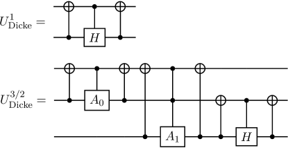
Figure 1: Circuit representations of the Dicke unitary operators $U_{\rm Dicke}^{S=1}$ and $U_{\rm Dicke}^{S=3/2}$. The Hadamard gate is denoted by $H$. In the circuit for $U_{\rm Dicke}^{S=3/2}$, the single-qubit $A_{0}$ gate is defined in matrix form as $A_{0}=\left(\begin{smallmatrix}1&-\sqrt{2}\\ \sqrt{2}&1\end{smallmatrix}\right)/\sqrt{3}$ and $A_{1}$ is defined as $A_{1}=\left(\begin{smallmatrix}\sqrt{2}&-1\\ 1&\sqrt{2}\end{smallmatrix}\right)/\sqrt{3}$. The $A_{k}$ gates are implemented in practice as $R_{Y}$ gates. The circuit diagrams in this manuscript are drawn using the Quantikz package [90].

II.3 Qubit Hamiltonians and Suzuki-Trotter approximation

The qubit form of the spin Hamiltonian (II.1) is expressed as

$$\mathcal{H}_{\rm q}=J\sum_{k=1}^{L}h_{k}P_{k},$$ (14)

where $h_{k}$ is an expansion coefficient, $P_{k}$, defined as

$$P_{k}=\sigma_{K_{\rm q}^{\rm tot}-1}^{k}\sigma_{K_{\rm q}^{\rm tot}-2}^{k}\cdots\sigma_{0}^{k},\qquad\sigma_{n}^{k}\in\{I,X,Y,Z\},$$ (15)

is a direct product of Pauli matrices, and $K_{\rm q}^{\rm tot}=NK_{\rm q}$ denotes the total number of qubits. For the compact and direct mappings, $\mathcal{H}_{\rm q}$ can be derived by applying the methods in [79] in a manner briefly described below. Taking the example of a two-site lattice for simplicity, we first write the spin Hamiltonian as

$$\mathcal{H}=\sum_{M^{\prime}_{1},M^{\prime}_{0},M_{1},M_{0}=-S}^{S}\eta_{M^{\prime}_{1}M^{\prime}_{0}M_{1}M_{0}}|M^{\prime}_{1}M^{\prime}_{0}\rangle\langle M_{1}M_{0}|,$$ (16)

where $\eta_{M^{\prime}_{1}M^{\prime}_{0}M_{1}M_{0}}$ are numerical values of the matrix elements derived by the application of Eqs. (3) and (4). Next, we convert $|M^{\prime}_{1}M^{\prime}_{0}\rangle\langle M_{1}M_{0}|$ to a qubit operator form using the mappings (5) or (7) and the identifications $|0\rangle\langle 0|=(I+Z)/2$, $|0\rangle\langle 1|=(X+iY)/2$, $|1\rangle\langle 0|=(X-iY)/2$, and $|1\rangle\langle 1|=(I-Z)/2$. In the case of the direct mapping, we only need to consider the part where the qubit state is changed. For example, for $S=1$, we map the matrix element $|M^{\prime}_{1}=-1,M^{\prime}_{0}=1\rangle\langle M_{1}=0,M_{0}=0|$ with $M_{1}\neq M^{\prime}_{1}$ and $M_{0}\neq M^{\prime}_{0}$ according to

$$|{-1},1\rangle\langle 0,0|={} |{001100}\rangle_{\rm q}{}_{\rm q}\langle{010010}|$$

$$={} \frac{1}{16}(X_{4}+iY_{4})(X_{3}-iY_{3})(X_{2}-iY_{2})$$

$$\quad\times(X_{1}+iY_{1}).$$ (17)

For the direct mapping, we find that the total number of terms $L$ for a two-site lattice is proportional to $S^{2}$ and that $L_{\rm direct}\approx 36S^{2}$ for $S$ in the range $1/2\leq S\leq 5$. For the compact mapping, we have not been able to analytically derive the scaling of $L$, but as discussed in detail in Appendix A, we find empirically that $L_{\rm compact}\propto S^{2.4}$ holds approximately for $S$ in the range $1/2\leq S\leq 63/2$.

In the case of the Dicke mapping, we simply replace each spin-$S$ operator $\hat{\bm{S}}$ in (II.1) by the total qubit spin operator $\hat{\bm{S}}_{\text{q}}=\frac{\hbar}{2}\sum_{k=0}^{K_{\rm q}-1}(X_{k},Y_{k},Z_{k})$ [67, 68] so that the qubit Hamiltonian becomes

$$\mathcal{H}_{\rm q}^{\rm Dicke}=\frac{J}{4}\sum_{(m,n)}\sum_{k=\kappa_{0}(m)}^{\kappa_{1}(m)}\sum_{l=\kappa_{0}(n)}^{\kappa_{1}(n)}W_{kl},$$ (18)

where

$$W_{kl}=Z_{k}Z_{l}+Y_{k}Y_{l}+X_{k}X_{l}.$$ (19)

In Eq. (18), $(m,n)$ labels a pair of interacting sites on the lattice and $k$ and $l$ denote the indices of the qubits describing the spin at sites $m$ and $n$, respectively. The qubit index $k$ at site $n$ takes values in the range $\kappa_{0}(n)\leq k\leq\kappa_{1}(n)$. For example, for a two-site $S=1$ system, the qubits 0 and 1 are assigned to site 0, meaning that $\kappa_{0}(0)=0$ and $\kappa_{1}(0)=1$, and qubits 2 and 3 are assigned to site 1, meaning that $\kappa_{0}(1)=2$ and $\kappa_{1}(1)=3$. The two-site, $S=1$ qubit Hamiltonian becomes

$$\mathcal{H}_{{\rm q},S=1}^{\rm Dicke}=\frac{J}{4}\sum_{k=0}^{1}\sum_{l=2}^{3}W_{kl}.$$ (20)

The total number of terms $L$ for a two-site lattice is $L_{\text{Dicke}}=12S^{2}$.

In the case of the qudit mapping, we write the Hamiltonian in terms of generalized Gell-Mann matrices [91],

$$\mathcal{H}_{d}=J\sum_{j=1}^{L}g_{k}\Gamma_{k},$$ (21)

where the $g_{k}$’s are expansion coefficients and $\Gamma_{k}$, defined as

$$\Gamma_{k}=\gamma^{k}_{N-1}\gamma^{k}_{N-2}\cdots\gamma^{k}_{0},\qquad\gamma_{n}^{k}\in\{\lambda_{0},\ldots,\lambda_{d^{2}-1}\},$$ (22)

is a direct product of $d\times d$ generalized Gell-Mann matrices $\lambda_{k}$. The detailed definition of $\lambda_{k}$ is given in Appendix B. Experimentally, implementation of the unitary operators $e^{i\theta\lambda_{k}}$ on a trapped-ion type quantum computer have been demonstrated in [89]. We find that for a two-site lattice, the number of terms in the Hamiltonian in the qudit mapping is the same as in the Dicke mapping, that is, $L_{\text{qudit}}=L_{\text{Dicke}}=12S^{2}$.

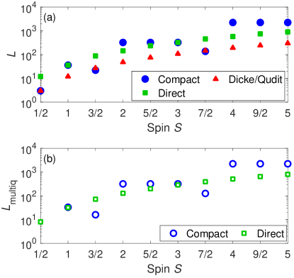
Figure 2: (a) Total number of terms $L$ in the two-site Hamiltonian (14) for the compact, direct, Dicke, and qudit mappings. Note that $L_{\text{Dicke}}=L_{\text{qudit}}$ and that the vertical axis is in the logarithmic scale. (b) The number of multi-qubit terms in the Hamiltonian. The Dicke Hamiltonian (18) and the qudit Hamiltonian (21) contain only two-qubit/qudit terms, and therefore, $L^{\text{multiq}}_{\text{Dicke}}=L^{\text{multiq}}_{\text{qudit}}=0$.

In Fig. 2(a), we show the total number of terms $L$ in the two-site qubit Hamiltonian using the compact, direct, Dicke, and qudit mappings. We can see that the Dicke mapping almost always results in a smaller $L$ than the compact or direct mappings. The only exception is when $2S+1$ is exactly equal to a power of 2, which occurs at $S=1/2$, $3/2$, and $7/2$ in Fig. 2. In these cases, all available qubit states correspond to spin states in the compact mapping, leading to a particularly compact representation of the qubit Hamiltonian [79]. However, even if the total number of terms $L$ is approximately the same in the Dicke and compact mappings for $S=1/2$, $3/2$, and $7/2$, the Dicke mapping Hamiltonian (18) contains only two-qubit operators, while the compact mapping Hamiltonian contains many operators acting on more than two qubits. For example, at $S=3/2$, the compact-mapping qubit Hamiltonian contains $L_{\rm compact}=22$ terms: six two-qubit operators, eight three-qubit operators, and eight four-qubit operators. At $S=2$, we have $L_{\rm compact}=324$ terms, out of which six are two-qubit operators, 28 are three-qubit operators, 73 are four-qubit operators, 118 are five-qubit operators, and 99 are six-qubit operators. In Fig. 2(b), we show the number $L_{\text{multiq}}$ of multi-qubit terms in the Hamiltonian, where a multi-qubit term is defined as an operator which acts on more than two qubits (or qudits in the case of the qudit mapping). The absence of operators acting on more than two qubits makes the Dicke mapping the most efficient spin-qubit mapping for the Suzuki-Trotter time evolution, as will be shown in Sec. III.

In order to propagate the wave function forward in time, we adopt the simplest form of the Suzuki-Trotter approximation [92, 93],

$$|\psi(t=N_{\rm ST}\Delta t)\rangle\approx\left[U_{\rm ST}(\Delta\tau)\right]^{N_{\rm ST}}|\psi_{0}\rangle,$$ (23)

where $|\psi_{0}\rangle$ is the initial state, $N_{\rm ST}$ is the number of Suzuki-Trotter steps,

$$U_{\rm ST}(\Delta\tau)=e^{-i\Delta\tau h_{k}P_{k}}e^{-i\Delta\tau h_{k-1}P_{k-1}}\cdots e^{-i\Delta\tau h_{1}P_{1}}$$ (24)

is the unitary operator of one Suzuki-Trotter step, and $\Delta\tau=J\Delta t/\hbar$ is the dimensionless time step. For the qudit mapping, an expression equivalent to Eq. (24) is used where the qubit operators $P_{k}$ are replaced by qudit operators $\Gamma_{k}$.

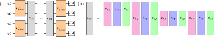
Figure 3: (a) Structure of the Suzuki-Trotter circuit for the Dicke mapping of a two-site, $S=1$ system. The qubits are initialized in the state $|\psi_{0}\rangle=|q_{3}q_{2}q_{1}q_{0}\rangle$. (b) Structure of one Suzuki-Trotter step $U_{\rm ST}$. The two-qubit rotation gates $R_{\alpha\alpha}$ with $\alpha=X$, $Y$, or $Z$ are defined as $R_{\alpha\alpha}=\exp\left(-i\frac{\Delta\tau}{4}\alpha\alpha\right)$. Each gate $R_{\alpha\alpha}$ operates on the two qubits covered by the colored rectangle.

In the case of the Dicke mapping, it is necessary to add the Dicke operator $U_{\rm Dicke}^{S}$ before the Suzuki-Trotter time evolution and $U_{\rm Dicke}^{S\dagger}$ before the final measurement in order to transform a computational basis state (a state $|{q_{K_{\rm q}^{\rm tot}-1}\cdots q_{0}}\rangle_{\rm q}$ with $q_{k}\in\{0,1\}$) to a Dicke state and back. We illustrate the structure of the Suzuki-Trotter circuit for the Dicke mapping in Fig. 3. It can be seen in Fig. 3 that, although the Dicke mapping is compact, it requires the coupling of non-neighboring qubits. This means that quantum computers having an all-to-all qubit connectivity, such as trapped-ion [94, 95, 96] and neutral atom [97] devices are particularly well suited for the practical realization of the Dicke mapping.

III Results

III.1 Comparison of compact, direct, Dicke, and qudit mappings

In order to assess the performance of the different mappings introduced in Secs. II.2 and II.3, we simulate the spin dynamics of a two-site lattice described by the Heisenberg Hamiltonian (II.1). We conduct the simulation at two values of the spin $S$, $S=1$ and $S=3/2$. The time-dependent wave function $|\psi(t)\rangle$ is calculated according to Eq. (23) for a fixed time step $\Delta\tau=0.2$ and the number of Suzuki-Trotter steps varying in the range $0\leq N_{\rm ST}\leq 31$, corresponding to a time range of $0\leq Jt/\hbar\leq 6.2$. We adopt the initial wave function $|\psi(t=0)\rangle=|M_{1}=-S,M_{0}=S\rangle$ and evaluate the time-dependent population $p_{0}(t)$ in the initial state,

$$p_{0}(t)=|\langle\psi(0)|\psi(t)\rangle|^{2}.$$ (25)

The initial-state population $p_{0}(t)$ depends on time because the initial state $|{-S},S\rangle$ is not an eigenstate of $\mathcal{H}$.

For the compact, direct, and Dicke mappings, we carry out the simulation using Quantinuum’s H1-1 trapped-ion type quantum computer [78], which has 20 qubits realized by 20 trapped ¹⁷¹Yb⁺ ions. The qubit states $|0\rangle$ and $|1\rangle$ are implemented as the states ${}^{2}S_{1/2}(F=0,m_{F}=0)$ and ${}^{2}S_{1/2}(F=1,m_{F}=0)$ of Yb⁺ [95]. At the time of the simulations (July, August and October, 2024), the single and two-qubit gate errors $\epsilon_{\rm 1q}$ and $\epsilon_{\rm 2q}$ of H1-1 were $\epsilon_{\rm 1q}\approx 2\times 10^{-5}$ and $\epsilon_{\rm 2q}\approx 1\times 10^{-3}$, respectively [78]. We have also used the H1-1 emulator, which implements an error model [98] closely mimicking the noise in the real H1-1 device. The parameters of the H1-1 emulator can be found in the documentation available at [99]. In the simulations using the H1-1 (real device and emulator), we have repeated the execution of each circuit $N_{\text{shot}}=1024$ times in order to estimate the populations.

For the qudit mapping, we have employed a noise model in which the qudit density matrix $\rho$ after each two-qudit gate is subject to a completely depolarizing noise channel

$$\rho\to\rho^{\prime}=(1-\epsilon_{\rm 2q})\rho+\frac{\epsilon_{\rm 2q}}{d^{2}}I_{d^{2}\times d^{2}},$$ (26)

where $I_{d^{2}\times d^{2}}$ is the identity matrix. We have conducted simulations using two values of the two-qudit gate error, $\epsilon_{\rm 2q}=1\times 10^{-3}$, which equals the two-qubit gate error of Quantinuum’s H1-1 [78], and $\epsilon_{\rm 2q}=1\times 10^{-2}$, which is a more realistic assumption of the two-qudit gate error achievable in the present qudit systems. Note that a gate error of $\epsilon_{\rm 2q}=3\times 10^{-2}$ was reported in [89] for the two-qudit Mølmer-Sørensen gate.

In Fig. 4, we show the initial-state population $p_{0}(t)$ for an $S=1$ two-site lattice, obtained by the compact, direct, Dicke, and qudit mappings. For reference, the explicit expressions of the qubit and qudit Hamiltonians are given in Appendix C. The number of qubits employed for the two sites is $2K_{\rm q}=4$ for the compact and Dicke mappings, and $2K_{\rm q}=6$ for the direct mapping. When the circuits are transpiled (using tket [100]), the total number of $R_{ZZ}$ gates (H1-1’s native two-qubit gate) for one Suzuki-Trotter step is $N_{\text{2q}}=63$ for the direct mapping, $N_{\text{2q}}=56$ for the compact mapping, and $N_{\text{2q}}=16$ (including $U_{\rm Dicke}^{1}$ and $U_{\rm Dicke}^{1\dagger}$) for the Dicke mapping. For the qudit mapping, the number of two-qutrit gates is the same as the number of terms in the Hamiltonian, $N_{\text{2q}}=L_{\rm Dicke}=12$.

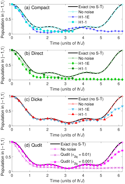
Figure 4: Populations in the $|M_{1},M_{0}\rangle=|{-1},1\rangle$ state for the Suzuki-Trotter simulation of a two-site, $S=1$ lattice obtained using the (a) compact, (b) direct, (c) Dicke, and (d) qudit mappings. The initial state is $|\psi(0)\rangle=|{-1},1\rangle$. In all plots, the exact populations obtained without using the Suzuki-Trotter approximation are drawn by black solid lines and the populations obtained by the Suzuki-Trotter approximation in the absence of noise are shown with open symbols. The curves in (a)–(c) labeled by “H1-1” are obtained by Quantinuum’s H1-1 trapped-ion quantum computer and the curves labeled by “H1-1E” are obtained by using the H1-1 emulator. The standard deviation estimated by bootstrapping [101] is smaller than 0.02 for all data points in all panels. Error bars are not shown because they are smaller than the curve symbols.

We can see in Figs. 4(a) and (b) that, in the case of the compact and direct mappings, $p_{0}(t)$ obtained using H1-1 starts deviating from $p_{0}(t)$ obtained in the absence of noise already in the early propagation time range of $Jt/\hbar>0.2$. On the other hand, $p_{0}(t)$ obtained using the Dicke and qudit mapping (with the smaller two-qutrit gate error $\epsilon_{\rm 2q}=1\times 10^{-3}$) shown in Fig. 4(c) and (d) agree well with the “No noise” curves. If we define the average error in the population as

$$\overline{\varepsilon}=\frac{1}{N_{\rm p}}\sum_{t_{n}\leq T}|p_{0}^{\text{(noisy)}}(t_{n})-p_{0}^{\text{(no noise)}}(t_{n})|,$$ (27)

where $t_{n}$ ($n=1,\ldots,N_{\rm p}$) are the time instants for the data shown in Fig. 4, we obtain $\overline{\varepsilon}_{\text{Dicke}}(\text{H1-1})=0.012$ and $\overline{\varepsilon}_{\text{qudit}}(\epsilon_{\rm 2q}=0.001)=0.011$ for $T=3.2\hbar/J$, much smaller than $\overline{\varepsilon}_{\text{compact}}(\text{H1-1})=0.080$ and $\overline{\varepsilon}_{\text{direct}}(\text{H1-1})=0.060$. The average error $\overline{\varepsilon}_{\text{qudit}}(\epsilon_{\rm 2q}=0.01)=0.081$ obtained in the qudit simulation using the larger value $\epsilon_{\rm 2q}=0.01$ of the two-qutrit gate error is comparable to the average errors obtained by the compact and direct mappings.

We also learn from Fig. 4 that the H1-1E emulator provides a rather accurate error model capable of reproducing the results obtained on the real H1-1 device.

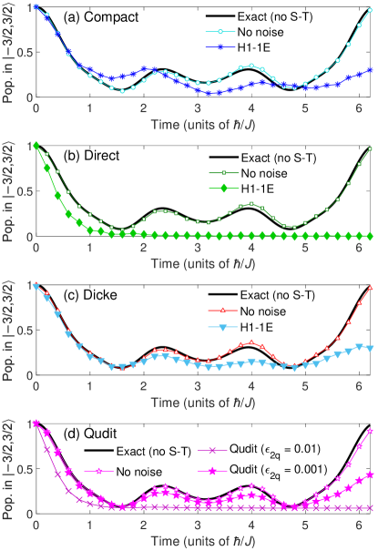
Figure 5: Populations in the $|M_{1},M_{0}\rangle=|{-3/2},3/2\rangle$ state for the Suzuki-Trotter simulation of a two-site, $S=3/2$ lattice obtained using the (a) compact, (b) direct, (c) Dicke, and (d) qudit mappings. The initial state is $|\psi(0)\rangle=|{-3/2},3/2\rangle$. The exact populations obtained without using the Suzuki-Trotter approximation are plotted by black solid lines and the populations obtained by the Suzuki-Trotter approximation in the absence of noise are plotted with open symbols. The curves in (a)–(c) labeled by “H1-1E” are obtained using Quantinuum’s H1-1 emulator. The error bars are everywhere smaller than the size of the curve symbols (the standard deviation as estimated by bootstrapping is smaller than 0.02) and are not shown.

In order to compare the different mappings when $L_{\rm compact}<L_{\rm Dicke}$, we show $p_{0}(t)$ in Fig. 5 for a two-site lattice with $S=3/2$. In this case, $L_{\rm compact}=22$ and $L_{\rm Dicke}=27$. The qubit Hamiltonians are shown in Appendix D. The number of qubits is $2K_{\rm q}=4$ for the compact mapping, $2K_{\rm q}=6$ for the Dicke mapping, and $2K_{\rm q}=8$ for the direct mapping. After transpiling the Suzuki-Trotter circuits to the native gates of H1-1 ($R_{ZZ}$, $R_{X}$, and $R_{Z}$), the number of two-qubit gates for one Suzuki-Trotter step becomes $N_{\text{2q}}=41$ for the compact mapping, $N_{\text{2q}}=143$ for the direct mapping, and $N_{\text{2q}}=49$ for the Dicke mapping. In the qudit mapping, we have $N_{\text{2q}}=L_{\rm Dicke}=27$ two-ququart gates. We use the emulator H1-1E to obtain the results shown in Fig. 5, but as we have shown in Fig. 4, we may expect similar results on the real H1-1 device.

We observe in Fig. 5 that, similarly to the case of $S=1$, $p_{0}(t)$ obtained using the Dicke and qudit ($\epsilon_{\rm 2q}=0.001$) mappings shown in Fig. 5(c) and (d) deviate only slightly from the noise-free populations. We obtain $\overline{\varepsilon}_{\text{Dicke}}(\text{H1-1E})=0.036$ and $\overline{\varepsilon}_{\text{qudit}}(\epsilon_{\rm 2q}=0.001)=0.030$ for the average errors, using $T=3.2\hbar/J$ in Eq. (27). The population obtained using the direct mapping shown in Fig. 5(b) and the qudit mapping with $\epsilon_{\rm 2q}=0.01$ shown in Fig. 5(d) rapidly decrease to the values $p_{0}(Jt/\hbar>2)\approx 1/2^{8}\approx 0.039$ for the direct mapping and $p_{0}(Jt/\hbar>2)\approx 1/4^{2}\approx 0.063$ for the qudit mapping with $\epsilon_{\rm 2q}=0.01$. This implies that, because of the error accumulation, a completely mixed state where all states are equally populated is produced where the value of $p_{0}$ is given by the inverse of the total number of qubit/qudit states. The average errors are therefore large, $\overline{\varepsilon}_{\text{direct}}(\text{H1-1E})=0.16$ and $\overline{\varepsilon}_{\text{qudit}}(\epsilon_{\rm 2q}=0.01)=0.14$. Because of the small number of terms in the Hamiltonian, the simulation employing the compact mapping results in rather accurate values of $p_{0}(t)$ as can be seen in Fig. 5(a). We obtain $\overline{\varepsilon}_{\text{compact}}(\text{H1-1E})=0.069$, which is only about a factor of two larger than $\overline{\varepsilon}_{\text{Dicke}}(\text{H1-1E})$.

From the comparison of the different mappings shown in Figs. 4 and 5, we conclude that both the Dicke mapping and the qudit mapping give equally accurate results, provided that a small two-qudit gate error of $\epsilon_{\rm 2q}=0.001$ can be achieved. This suggests that there is no particular advantage of simulating large-$S$ systems using qudit devices. On the other hand, the Dicke mapping is an efficient way of simulating large-$S$ lattices using quantum computers having an all-to-all qubit connectivity such as trapped-ion [96] and neutral atom [97] devices.

III.2 Dicke mapping for $1/2\leq S\leq 5/2$

In order to assess the performance of the Dicke mapping for a larger number of qubits, we simulate a four-site open-ended linear lattice, meaning that the sum over $(m,n)$ in Eq. (II.1) is taken over $(m,n)=(0,1)$, $(1,2)$ and $(2,3)$, for $S=1/2$, $1$, $3/2$, $2$, and $5/2$. The simulations are run on Quantinuum’s H1-1 trapped ion quantum computer [78] using $N_{\text{shot}}=1024$. Because $K_{\rm q}=2S$ qubits per site are required in the Dicke mapping, all the 20 qubits of H1-1 are employed in the $S=5/2$ simulation. The time step adopted in the Suzuki-Trotter approximation (24) is $\Delta\tau=\pi/10\approx 0.314$ and the number of Suzuki-Trotter time steps employed is proportional to $t$ according to $N_{\rm ST}=Jt/(\hbar\Delta\tau)$.

After transpilation with tket [100], the number of two-qubit gates in the quantum circuits for one Suzuki-Trotter step (including $U_{\rm Dicke}^{S}$ and $U_{\rm Dicke}^{S\dagger}$) becomes $N_{\text{2q}}(S=1/2)=8$, $N_{\text{2q}}(S=1)=44$, $N_{\text{2q}}(S=3/2)=125$, $N_{\text{2q}}(S=2)=252$, and $N_{\text{2q}}(S=5/2)=425$ for the different values of $S$. The longest circuit is a 20-qubit circuit for $S=5/2$ with $N_{\rm ST}=11$ Suzuki-Trotter steps ($Jt/\hbar=3.46$), resulting in $N_{\text{2q}}=2675$ two-qubit gates.

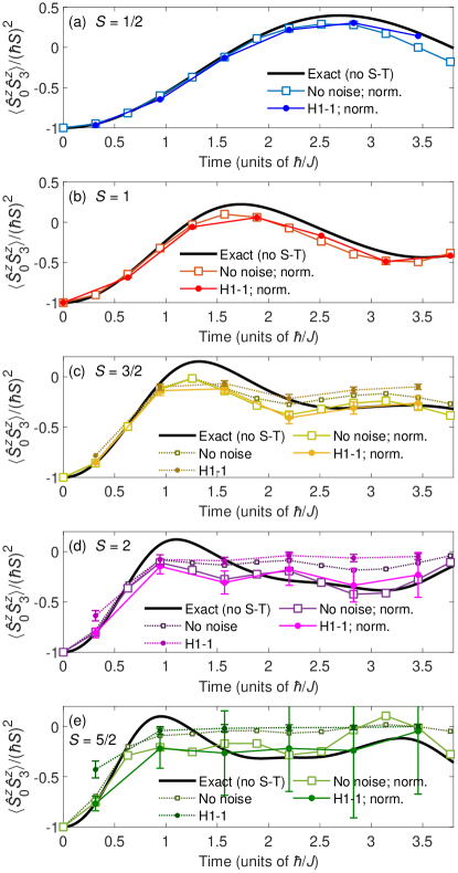
Figure 6: The time-dependent expectation value $\langle\hat{S}_{0}^{z}\hat{S}_{3}^{z}\rangle(t)$ for a four-site linear lattice, as defined in Eq. (28), for (a) $S=1/2$, (b) $S=1$, (c) $S=3/2$, (d) $S=2$, and (e) $S=5/2$. We show the exact results (labeled “Exact (no S-T)”), the results obtained using the Suzuki-Trotter approximation in the absence of noise (“No noise”), and the results obtained using Quantinuum’s H1-1. Curves labeled by “norm” are obtained after the post-selection and normalization as defined in Eq. (32). Because the effect of the post-selections is small in (a) and (b) (|$\langle\hat{S}_{0}^{z}\hat{S}_{3}^{z}\rangle-\langle\hat{S}_{0}^{z}\hat{S}_{3}^{z}\rangle_{\rm norm}|<0.03$ in (a) and |$\langle\hat{S}_{0}^{z}\hat{S}_{3}^{z}\rangle-\langle\hat{S}_{0}^{z}\hat{S}_{3}^{z}\rangle_{\rm norm}|<0.15$ in (b)), we show only the curves after the post-selection. The error bars represent one standard deviation and are shown only when the standard deviation exceeds $0.03$.

In Fig. 6, we show the time-dependent two-site observable

$$\langle\hat{S}_{0}^{z}\hat{S}_{3}^{z}\rangle(t)=\langle\psi(t)|\hat{S}_{0}^{z}\hat{S}_{3}^{z}|\psi(t)\rangle,$$ (28)

where $|\psi(t)\rangle$ is the time-dependent wave function evaluated using the Suzuki-Trotter approximation (23) with $\Delta\tau=\pi/10\approx 0.314$. The initial state is

$$|\psi(t=0)\rangle=|M_{3}=-S,M_{2}=-S,M_{1}=-S,M_{0}=S\rangle.$$ (29)

In order to facilitate the comparison of $\langle\hat{S}_{0}^{z}\hat{S}_{3}^{z}\rangle$ evaluated for the different values of $S$, we show the scaled quantity $\langle\hat{S}_{0}^{z}\hat{S}_{3}^{z}\rangle/(\hbar S)^{2}$ in Fig. 6.

In practice, we evaluate $\langle\hat{S}_{0}^{z}\hat{S}_{3}^{z}\rangle(t)$ according to

$$\langle\hat{S}_{0}^{z}\hat{S}_{3}^{z}\rangle\approx\sum_{\vec{M}}M_{0}M_{3}\frac{N_{\vec{M}}}{N_{\text{shot}}},$$ (30)

where $N_{\vec{M}}$ is the number of measurements of a qubit state representing a spin state $|\vec{M}\rangle$. This means that the sum in Eq. (30) is taken only over qubit states which are mapped to the spin states by $U_{\rm Dicke}^{S}$. For example, for $S=1$, the sum in Eq. (30) includes the eight-qubit states $|Q_{3}Q_{2}Q_{1}Q_{0}\rangle$ with $Q_{i}\in\{00,01,11\}$.

We also show in Fig. 6 the result of a simple form of error mitigation by the post-selection and renormalization explained as follows. Because of the error in the Suzuki-Trotter approximation (23), the total population in the qubit states representing Dicke states decreases and becomes smaller than one even in the absence of noise. The only exception is $S=1/2$, in which the Dicke state population is conserved because $K_{\rm q}=1$, meaning that all qubit states represent a Dicke state. In addition, because of the noise, the total magnetic quantum number

$$M_{\rm tot}=\sum_{n=0}^{N-1}M_{n}$$ (31)

is not conserved during the simulation, even though the Hamiltonian $\mathcal{H}$ commutes with $\hat{S}_{\text{tot}}^{z}=\sum_{n=0}^{N-1}\hat{S}_{n}^{z}$. Therefore, even if we start the simulation in the state (29) having $M_{\rm tot}=-2S$, the total population summed over all states having the same $M_{\rm tot}$ decreases during the Suzuki-Trotter simulation. A simple way of error mitigation is to post-select only the spin states having the same $M_{\rm tot}$ as the initial state, and renormalize their population to one before calculating the expectation value,

$$\langle\hat{S}_{0}^{z}\hat{S}_{3}^{z}\rangle_{\text{norm}}=\sum_{\vec{M}:M_{\rm tot}=M^{\text{i}}_{\rm tot}}M_{0}M_{3}\frac{N_{\vec{M}}}{N_{M^{\text{i}}_{\rm tot}}},$$ (32)

where $M^{\text{i}}_{\rm tot}$ is the total magnetic number of the initial state ($=2S$ in Fig. 6), and $N_{M^{\text{i}}_{\rm tot}}$ is the total number of measurements of qubit states corresponding to the spin states whose total magnetic quantum numbers equal $M^{\text{i}}_{\rm tot}$. The error-mitigated values of $\langle\hat{S}_{0}^{z}\hat{S}_{3}^{z}\rangle$ evaluated according to Eq. (32) are shown with solid lines (labeled “norm”) in Fig. 6. For reference, we give the total population $p_{M_{\rm tot}}$ in the states with $M_{\rm tot}=M^{\text{i}}_{\rm tot}$ as estimated by $p_{M_{\rm tot}}=N_{M^{\text{i}}_{\rm tot}}/N_{\text{shot}}$ at the largest $t=t_{\rm max}$ attempted in the H1-1 simulations ($Jt_{\rm max}/\hbar=3.77$ for $S=1$, and $Jt_{\rm max}/\hbar=3.46$ for $S\neq 1$). For the noise-free simulations, we have $p_{M_{\rm tot}}^{S=1/2}(t_{\rm max})=1$, $p_{M_{\rm tot}}^{S=1}(t_{\rm max})=0.909$, $p_{M_{\rm tot}}^{S=3/2}(t_{\rm max})=0.691$, $p_{M_{\rm tot}}^{S=2}(t_{\rm max})=0.402$, and $p_{M_{\rm tot}}^{S=5/2}(t_{\rm max})=0.161$, and for the simulations conducted using H1-1, we have $p_{M_{\rm tot}}^{S=1/2}(t_{\rm max})=0.959$, $p_{M_{\rm tot}}^{S=1}(t_{\rm max})=0.665$, $p_{M_{\rm tot}}^{S=3/2}(t_{\rm max})=0.331$, $p_{M_{\rm tot}}^{S=2}(t_{\rm max})=0.0898$, and $p_{M_{\rm tot}}^{S=5/2}(t_{\rm max})=0.0195$. Because of the small values of $p_{M_{\rm tot}}^{S}(t_{\rm max})$ for large $S$, the error bars of the error-mitigated H1-1 curves become large, as can be seen for $S=5/2$ in Fig. 6(e).

We can see in Fig. 6 that $\langle\hat{S}_{0}^{z}\hat{S}_{3}^{z}\rangle$ obtained using H1-1 agrees well with the noise-free curves for $S<5/2$. For the largest spin considered, $S=5/2$, the effect of the noise is too large to obtain a meaningful result after error mitigation. We also see that, for $S<5/2$, the renormalized noise-free curves provide reasonable approximations to the exact curves, showing that the error mitigation scheme of the post-selection and renormalization is a simple and efficient way of reducing the effect of the population decrease in the Dicke states.

A characteristic feature of the curves in Fig. 6 is that $\langle\hat{S}_{0}^{z}\hat{S}_{3}^{z}\rangle/(\hbar S)^{2}$ increases faster with time as $S$ increases. This observation can be explained by second-order perturbation theory. After some algebra, we derive for small $Jt/\hbar\ll 1$

$$\frac{\langle\hat{S}_{0}^{z}\hat{S}_{3}^{z}\rangle(t)}{\hbar^{2}S^{2}}\approx\frac{\langle\psi_{\rm PT2}(t)|\hat{S}_{0}^{z}\hat{S}_{3}^{z}|\psi_{\rm PT2}(t)\rangle}{\hbar^{2}S^{2}}=-1+S\left(\frac{Jt}{\hbar}\right)^{2},$$ (33)

where the wave function up to the second order in $t$ is calculated according to

$$|\psi_{\rm PT2}(t)\rangle=\left(1-\frac{it}{\hbar}\mathcal{H}-\frac{t^{2}}{2\hbar^{2}}\mathcal{H}^{2}\right)|-S,-S,-S,S\rangle.$$ (34)

Equation (33) shows that the second time derivative (the acceleration) of $\langle\hat{S}_{0}^{z}\hat{S}_{3}^{z}\rangle/(\hbar S)^{2}$ is proportional to $S$ for small $t$, which explains the fast increase of $\langle\hat{S}_{0}^{z}\hat{S}_{3}^{z}\rangle/(\hbar S)^{2}$ for large $S$.

III.3 Time step size in the Suzuki-Trotter approximation

As is clear from the comparison of the “Exact” and “No noise” results shown in Fig. 6, the discrepancy between the exact results obtained without using the Suzuki-Trotter approximation and the (noise-free) results obtained using the Suzuki-Trotter approximation increases as $S$ increases. Because the same value of the Suzuki-Trotter step size $\Delta\tau=0.314$ is used for all values of $S$ in Fig. 6, this suggests that, in order to obtain equally accurate results for all $S$, a smaller value of $\Delta\tau$ should be selected for large $S$.

In order to investigate how small $\Delta\tau$ should be for different values of $S$, we evaluate the final spin-state population of a two-site lattice at $Jt/\hbar=1$,

$$p_{\vec{M}^{\rm f}\vec{M}^{\rm i}}(t=\hbar/J)=\left|\langle\vec{M}^{\rm f}|\left[U_{\rm ST}(\Delta\tau=N_{\rm ST}^{-1})\right]^{N_{\rm ST}}|\vec{M}^{\rm i}\rangle\right|^{2},$$ (35)

where $|\vec{M}^{\rm i}\rangle=|M^{\text{i}}_{1},M^{\text{i}}_{0}\rangle$ and $|\vec{M}^{\text{f}}\rangle=|M^{\text{f}}_{1},M^{\text{f}}_{0}\rangle$ are the initial and final spin states, respectively, and the Suzuki-Trotter time-evolution operator $U_{\rm ST}$ is constructed using the Dicke mapping. We also evaluate the exact final population obtained without using the Suzuki-Trotter approximation,

$$p^{\text{exact}}_{\vec{M}^{\rm f}\vec{M}^{\rm i}}(t=\hbar/J)=\left|\langle\vec{M}^{\rm f}|e^{-i\mathcal{H}/J}|\vec{M}^{\rm i}\rangle\right|^{2},$$ (36)

and define the average discrepancy $\overline{\Delta}$ as the difference between $p_{\vec{M}^{\rm f}\vec{M}^{\rm i}}$ and $p^{\text{exact}}_{\vec{M}^{\rm f}\vec{M}^{\rm i}}$ averaged over all initial and final states,

$$\overline{\Delta}(t=\hbar/J)=\frac{1}{\zeta(S)}\sum_{\vec{M}^{\rm i},\vec{M}^{\rm f}}\left|p_{\vec{M}^{\rm f}\vec{M}^{\rm i}}(\hbar/J)-p^{\text{exact}}_{\vec{M}^{\rm f}\vec{M}^{\rm i}}(\hbar/J)\right|,$$ (37)

where $\zeta(S)=(2S+1)[1+2(2S+1)^{2}]/3$ is the total number of terms and only final states having the same $M_{\text{tot}}$ as the initial state are included in the sum over $\vec{M}^{\rm f}$. The reason to use $\overline{\Delta}$ defined in Eq. (37) as the measure of the discrepancy instead of the wave function fidelity or the matrix norm is that the expression (37) is straightforwardly evaluated on a NISQ device or using a noise model.

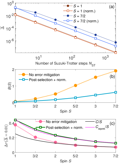
Figure 7: (a) The average difference $\overline{\Delta}(t=\hbar/J)$ between the final spin-state population evaluated using the Suzuki-Trotter approximation in the absence of noise and the exact populations defined in Eq. (37). The curves labeled by “norm.” are calculated by populations whose error is mitigated by the post-selection and renormalization defined in Eq. (38). (b) Proportionality constant $B(S)$ in the fit $\overline{\Delta}=B(S)/N_{\rm ST}^{2}$. (c) Time step size $\Delta\tau$ required to achieve an average discrepancy $\overline{\Delta}=0.01$. The filled circles and open squares are obtained using the data in (b) and Eq. (43), and the solid lines are least-squares fits to $\Delta\tau=C/S$ with $C=0.254$ and $C_{\rm norm}=0.453$.

We first evaluate $\overline{\Delta}(t=\hbar/J)$ in the ideal case of no noise. In Fig. 7(a), we show $\overline{\Delta}(t=\hbar/J)$ for a varying number of time steps $N_{\rm ST}=2^{x}$ with $x=1,3,\ldots,11$. We show the results for two values of $S$, $S=1$ and $S=7/2$. Because of the Suzuki-Trotter approximation, $M_{\text{tot}}$ is not conserved in the Dicke mapping, and we have in general $\sum_{\vec{M}^{\rm f}}p_{\vec{M}^{\rm f}\vec{M}^{\rm i}}<0$ for the total final population. Note however that, in the noise-free case, the population leaks to qubit states not representing spin states and not to spin states with $M_{\rm tot}^{\rm f}\neq M_{\rm tot}^{\rm i}$. In other words, we have $p_{\vec{M}^{\rm f}\vec{M}^{\rm i}}=0$ for $\vec{M}^{\rm f}\neq\vec{M}^{\rm i}$. As discussed in Sec. III.2, simple form of error mitigation consists of the renormalization of $p_{\vec{M}^{\rm f}\vec{M}^{\rm i}}$ to 1,

$$p^{\rm norm}_{\vec{M}^{\rm f}\vec{M}^{\rm i}}=\frac{p_{\vec{M}^{\rm f}\vec{M}^{\rm i}}}{\sum_{\vec{M}^{{}^{\prime}{\rm f}}}p_{\vec{M}^{{}^{\prime}{\rm f}}\vec{M}^{\rm i}}}.$$ (38)

The average discrepancy $\overline{\Delta}$ evaluated using $p^{\rm norm}_{\vec{M}^{\rm f}\vec{M}^{\rm i}}$ in (37) is labeled by “norm.” in Fig. 7(a). As clearly seen in Fig. 7(a), the post-selected and renormalized $\overline{\Delta}$ are smaller than $\overline{\Delta}$ without error mitigation, demonstrating that the post-selection can be used to mitigate the error in the Suzuki-Trotter approximation.

We can see in Fig. 7(a) that both the unmitigated $\overline{\Delta}$ and the mitigated $\overline{\Delta}$ are to a good approximation proportional to $1/N_{\rm ST}^{2}$ (note that Fig. 7(a) is plotted in the double logarithmic scale). We find the same $1/N_{\rm ST}^{2}$-dependence of $\overline{\Delta}$ also for other values of $S<7/2$, which are not shown in Fig. 7(a). The $1/N_{\rm ST}^{2}$-dependence of $\overline{\Delta}$ may seem surprising at first, because the Suzuki-Trotter approximation (24) is in general accurate to the first order in $\Delta\tau$, that is,

$$U_{\rm ST}(\Delta\tau)=e^{-i\Delta\tau\sum_{k}h_{k}P_{k}}+\mathcal{O}(\Delta\tau^{2}),$$ (39)

and we would therefore expect the error in the wave function after $N_{\rm ST}$ steps to be proportional to $\Delta\tau$ ($=1/N_{\rm ST}$). However, in the Dicke mapping, we have

$$e^{-i\Delta t\mathcal{H}_{\rm q}^{\rm Dicke}/\hbar}= \prod_{k,l}e^{-i\Delta\tau W_{kl}}$$

$$+\frac{\Delta\tau^{2}}{4}\sum_{kl,k^{\prime}l^{\prime}}[W_{kl},W_{k^{\prime}l^{\prime}}]+\mathcal{O}(\Delta\tau^{3}),$$ (40)

where $W_{kl}$ was defined in Eq. (19), $[\cdot,\cdot]$ is the commutator, and the sum in the second line is taken over qubit indices $kl$ and $k^{\prime}l^{\prime}$ for which either $k<k^{\prime}$ or $l<l^{\prime}$. Furthermore, we have

$${}_{\rm q}\langle{1_{S-M}}|U_{\rm Dicke}^{S\dagger}[W_{kl},W_{k^{\prime}l^{\prime}}]U_{\rm Dicke}^{S}|{1_{S-M}}\rangle_{\rm q}=0$$ (41)

for the Dicke operator defined in Eq. (12), because the commutator $[W_{kl},W_{k^{\prime}l^{\prime}}]$ is antisymmetric and the Dicke state $|{D_{S,M}}\rangle_{\rm q}=U_{\rm Dicke}^{S}|{1_{S-M}}\rangle_{\rm q}$ is symmetric with respect to the qubit indices $kl$ and $k^{\prime}l^{\prime}$. Equation (41) implies that the Suzuki-Trotter propagator $\prod_{k,l}e^{-i\Delta\tau W_{kl}}$ for one time step in the Dicke mapping is accurate to the second order in $\Delta\tau$ because the term proportional to $\Delta\tau^{2}$ in Eq. (III.3) vanishes, and consequently, the error after $N_{\rm ST}$ steps becomes proportional to $\Delta\tau^{2}=1/N_{\rm ST}^{2}$.

The average discrepancy $\overline{\Delta}$ in Fig. 7(a) can be fitted with

$$\overline{\Delta}=\frac{B}{N_{\rm ST}^{2}},$$ (42)

where $B$ is a fitting parameter. The resulting $S$-dependent $B(S)$ is shown in Fig. 7(b). We can see that $B(S)$ increases with increasing $S$ and that $B(S)$ obtained from the post-selected populations is smaller than the unmitigated $B(S)$ by a factor of two to three. Equation (42) can be used to obtain the time step $\Delta\tau$ required to achieve a certain average difference $\overline{\Delta}$ at $t=\hbar/J$,

$$\Delta\tau=\frac{1}{N_{\rm ST}}=\sqrt{\frac{\overline{\Delta}}{B}}.$$ (43)

The time step size $\Delta\tau$ for an average discrepancy of $\overline{\Delta}=0.01$ is shown in Fig. 7(c). We find that the value of $\Delta\tau$ decreases with increasing $S$ approximately as $\Delta\tau=C/S$ for the large $S\geq 2$. By fitting the data in Fig. 7 for $S\geq 2$ to $\Delta\tau=C/S$, we obtain $C=0.254$ and $C_{\rm norm}=0.453$.

The case of $S=1/2$ is not considered in Fig. 7 because the Suzuki-Trotter approximation is exact for a two-site, $S=1/2$ lattice. We have

$$e^{-it\mathcal{H}_{\rm q}^{\rm Dicke}/\hbar} =e^{-i\frac{Jt}{4\hbar}(X_{1}X_{0}+Y_{1}Y_{0}+Z_{1}Z_{0})}$$

$$=e^{-i\frac{Jt}{4\hbar}X_{1}X_{0}}e^{-i\frac{Jt}{4\hbar}Y_{1}Y_{0}}e^{-i\frac{Jt}{4\hbar}Z_{1}Z_{0}}$$ (44)

because the operators $X_{1}X_{0}$, $Y_{1}Y_{0}$, and $Z_{1}Z_{0}$ commute with each other.

In order to investigate the effect of the noise on $\overline{\Delta}$, we evaluate $\overline{\Delta}(t=\hbar/J)$ as a function of $N_{\rm ST}$ for $1\leq S\leq 5/2$ using the H1-1 emulator [99]. We employ $N_{\text{shot}}=1024$. The results of the simulation in which $N_{\text{shot}}=1024$ is chosen are shown in Fig. 8. For comparison, we also show the value of $\overline{\Delta}$ obtained by assuming a completely mixed final state where all qubit-states are equally populated, that is,

$$p_{\vec{M}^{\rm f}\vec{M}^{\rm i}}(t=\hbar/J)=\frac{1}{2^{2K_{\rm q}}}$$ (45)

for all $\vec{M}^{\rm f}$ and $\vec{M}^{\rm i}$, where $K_{\rm q}=2S$ is the number of qubits per lattice site. The average discrepancy $\overline{\Delta}_{\rm mix}$ obtained using Eq. (45) can be regarded as the worst case where the effect of the noise is very large. A successful simulation must result in a value of $\overline{\Delta}$ much smaller than $\overline{\Delta}_{\rm mix}$.

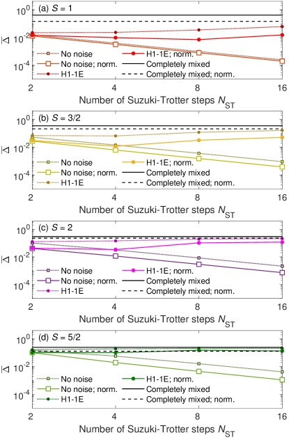
Figure 8: The average discrepancy $\overline{\Delta}$ as defined in Eq. (37) evaluated without noise (open squares) and with noise by the H1-1 emulator (filled circles) for (a) $S=1$, (b) $S=3/2$, (c) $S=2$, and (d) $S=5/2$. The error bars for the H1-1E curves estimated by bootstrapping are smaller than $0.01$ for all curves and are therefore not shown. The curves labeled by “norm” are the results obtained by the post-selection and normalization according to Eq. (38). The black horizontal lines represent the value of $\overline{\Delta}$ obtained by assuming a completely mixed state in which all the qubit states are equally populated.

In Fig. 8, we can see that the noise-free curves (open squares) decrease with $N_{\rm ST}$ as $\overline{\Delta}\propto 1/N_{\rm ST}^{2}$ for all the $S$ values. As can be seen in Figs. 8(a) ($S=1$) and 8(b) ($S=3/2$), the error-mitigated curves obtained using H1-1E decrease until an optimal value of $N_{\rm ST}=N_{\rm ST}^{\rm opt}$, but $\overline{\Delta}$ starts increasing when $N_{\rm ST}$ is further increased, showing that the simulation becomes less accurate. For the larger $S$ values, the situation becomes worse as shown in Figs. 8(c) and  8(d).

Because of the presence of the noise, there is a trade-off between the accuracy of the Suzuki-Trotter approximation which can be raised by increasing the number of Suzuki-Trotter steps $N_{\rm ST}$ and the effect of the noise which can also be raised by increasing $N_{\rm ST}$ associated with the increase in the depth of the quantum circuit. For the Dicke mapping applied to a two-site lattice the results shown in Fig. 8 obtained using the H1-1 emulator (two-qubit gate error $\epsilon_{\rm 2q}\approx 10^{-3}$) suggest that the optimal number of Suzuki-Trotter steps is $N_{\rm ST}^{\rm opt}\approx 8$ for $S=1$ and $N_{\rm ST}\approx 4$ for $S=3/2$. In the case of $S=2$, shown in Fig. 8(c), the average discrepancy for $N_{\rm ST}=2$, $\overline{\Delta}_{\text{H1-1E}}^{\text{norm.}}(N_{\rm ST}=2)=0.103$, is almost the same as that for $N_{\rm ST}=4$, $\overline{\Delta}_{\text{H1-1E}}^{\text{norm.}}(N_{\rm ST}=4)=0.102$, which means that the accuracy of the simulation is not improved by increasing the number of Suzuki-Trotter steps. In Fig. 8(d), we see that the average discrepancy $\overline{\Delta}$ obtained using H1-1 is close to the $\overline{\Delta}_{\rm mix}$ obtained from the completely mixed state and conclude that at the present two-qubit gate error ($\epsilon_{\rm 2q}\approx 10^{-3}$), $S=5/2$ is too large for accurate simulations on H1-1.

IV Summary

In the present study, we compared four different mappings of the Heisenberg model for a lattice of interacting spins with arbitrary $S$ to qubit or qudit form. We found that the Dicke mapping, in which the state of a spin-$S$ lattice site is described by a superposition of $2S$-qubit states, is the most efficient and accurate mapping, because the number of terms in the Hamiltonian is much smaller than that in the other qubit mapping schemes. The Dicke mapping was assessed by simulating two-site and four-site lattices with $S$ up to $5/2$ using Quantinuum’s trapped-ion quantum computer H1-1. Accurate time-dependent spin-state populations and expectation values were obtained for $S\leq 2$.

A qudit mapping scheme, in which each lattice site is described by a qudit having $2S+1$ levels, was found to result in an equally compact expression of the qudit Hamiltonian as the Dicke mapping. However, given that the gate errors of qudit devices are currently much larger than the gate errors of qubit devices, the good performance of the Dicke mapping suggests that the Dicke mapping is more suited for the simulation of large $S$ lattices than a qudit mapping.

A disadvantage of the Dicke mapping is that, after the application of the Suzuki-Trotter approximation, the total population in the Dicke states is no longer conserved even when a noise-free simulator is employed. To mitigate this non-conservation of the population, we suggested a simple error mitigation method based on the post-selection and renormalization. It was reported that the decrease in the population in the Dicke states can be mitigated by employing projection operators [77]. It is also possible that the conservation of the population can be improved by adopting more complex Suzuki-Trotter schemes similar to those reported in [102, 103].

Having established the efficiency of the Dicke mapping both theoretically and by simulations using current quantum hardware, we believe that the Dicke mapping will be a powerful tool in the quantum computing of large-$S$ lattices such as single-molecule magnets and molecular cluster complexes.

Appendix A Number of terms in the compact mapping Hamiltonian

Although very large values of $S>10$ are hardly useful in simulations, it is of theoretical interest to investigate the large-$S$ scaling of the number of terms $L$ in the qubit Hamiltonian. In the case of the compact mapping, an analytical formula of $L$ cannot be easily derived, and we have therefore carried out a numerical investigation for $1/2\leq S\leq 63/2$.

The number of terms $L_{\rm compact}$ in the compact-mapping qubit Hamiltonian for a two-site lattice is shown in Fig. 9 as a function of $S$. The number of qubits $K_{\rm q}$ required per site is indicated by the color and marker style. We can see that for values of $S$ requiring the same number of $K_{\rm q}$, $L_{\rm compact}$ is roughly constant. The exception is the last data point in each group at $2^{K_{\rm q}}=2S+1$, which means that all qubit states are used to represent spin states. In this case, $L_{\rm compact}$ is much smaller than at the other values of $S$ requiring the same $K_{\rm q}$.

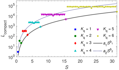
Figure 9: Number of terms $L_{\rm compact}$ in the compact mapping qubit Hamiltonian for a two-site lattice as a function of $S$. The data is grouped according to the required number of qubits per site $K_{\rm q}$. The least-squares fit $a_{1}S^{b_{1}}$ with $a_{1}=6.7$ and $b_{1}=2.4$ is shown by a solid line, and $a_{2}S^{b_{2}}$ with $a_{2}=35.1$ and $b_{2}=2.4$ ($=b_{1}$) is shown by a dotted line.

Even though we have not been able to derive an analytical formula for $L_{\rm compact}(S)$, we have found that $L_{\rm compact}$ in the range of $S$ shown in Fig. 9 can be well fitted by a power law. For $S$ satisfying $2S+1=2^{K_{\rm q}}$ ($K_{\rm q}=1,\ldots,6$), we have found that $L_{\rm compact}(S)\approx a_{1}S^{b_{1}}$ provides a good fit with $a_{1}=6.7$ and $b_{1}=2.4$. This curve is shown with a solid line in Fig. 9. In order to discuss the other values of $S$ where $\log_{2}(2S+1)$ are not an integer, we define the central value $S_{\rm c}$ for each $K_{\rm q}$,

$$S_{\rm c}=\begin{cases}\frac{1}{2},&\text{if }K_{\rm q}=1,\\ 3\times 2^{K_{\rm q}-3}-\frac{1}{2},&\text{otherwise},\end{cases}$$ (46)

and the average $\overline{L}_{\rm compact}(K_{\rm q})$ of $L_{\rm compact}(S)$ for $S$ corresponding to the same value of $K_{\rm q}$, excluding $S=2^{K_{\rm q}-1}-1/2$,

$$\overline{L}_{\rm compact}(K_{\rm q})=\begin{cases}L_{\rm compact}(1),&\text{if }K_{\rm q}=1,\\ {\displaystyle\frac{1}{2^{K_{\rm q}-1}}}{\displaystyle\sum_{S=2^{K_{\rm q}-2}}^{2^{K_{\rm q}-1}-1}}L_{\rm compact}(S),&\text{otherwise}.\end{cases}$$ (47)

We then fit $\overline{L}_{\rm compact}(K_{\rm q})$ by a power law of the form $a_{2}S_{\rm c}^{b_{2}}$, and find a good fit for $a_{2}=35.1$ and $b_{2}=2.4$. This fit is shown by a dotted line in Fig. 9. Note that the exponents for the solid and dotted lines in Fig. 9 are the same, $b_{1}=b_{2}$, which implies that both $L_{\rm compact}(S)$ with $S=2^{K_{\rm q}-1}-1/2$ and $L_{\rm compact}(S)$ with $S\neq 2^{K_{\rm q}-1}-1/2$ scale in the same way with increasing $S$.

Appendix B Generalized Gell-Mann matrices

The generalized $d\times d$ Gell-Mann matrices $\lambda_{k}$ ($k=1,2,\ldots,d^{2}$), which provide a convenient basis for $d\times d$ Hermitian matrices, are defined as follows [91]. $\lambda_{1}$ is defined as being proportional to the identity matrix,

$$(\lambda_{1})_{mn}=\sqrt{\frac{2}{d}}\delta_{mn},$$ (48)

where $\delta_{mn}$ is the Kronecker delta. The rest of the generalized Gell-Mann matrices are of three types: $X$-like, having matrix elements defined as

$$(\lambda_{k})_{mn}=\delta_{jm}\delta_{ln}+\delta_{jn}\delta_{lm},$$ (49)

and $Y$-like,

$$(\lambda_{k})_{mn}=-i\delta_{jm}\delta_{ln}+i\delta_{jn}\delta_{lm},$$ (50)

for all $j$ and $l$ in the range $1<j\leq d$, $1\leq l<j$, and diagonal $Z$-like matrices defined for all $1<j\leq d$ as

$$(\lambda_{k})_{mn}=\sqrt{\frac{2}{j(j-1)}}\Omega_{m}(j)\delta_{mn}$$ (51)

with

$$\Omega_{m}(j)=\begin{cases}1,&\text{if }1\leq m<j,\\ 1-j,&\text{if }m=j,\\ 0,&\text{if }m>j.\end{cases}$$ (52)

We order the generalized Gell-Mann matrices so that $\lambda_{2}$ corresponds to $j=2$, $l=1$ ($X$-like), $\lambda_{3}$ to $j=2$, $l=1$ ($Y$-like), $\lambda_{4}$ to $j=2$ ($Z$-like), $\lambda_{5}$ and $\lambda_{6}$ to $j=3$, $l=1$ ($X$ and $Y$-like), $\lambda_{7}$ and $\lambda_{8}$ to $j=3$, $l=2$ ($X$ and $Y$-like), $\lambda_{9}$ to $j=3$ ($Z$-like), and so on.

The generalized Gell-Mann matrices $\lambda_{k}$ satisfy $\operatorname{tr}(\lambda_{k})=0$ and $\operatorname{tr}(\lambda_{k}\lambda_{l})=2\delta_{kl}$. For $d=2$, they reduce to the standard Pauli matrices, and for $d=3$, they reproduce the original Gell-Mann matrices [104].

Appendix C Qubit and qudit Hamiltonians for $S=1$

The qubit form of the Hamiltonian for the compact mapping ($S=1$) is

$$\mathcal{H}_{\rm q}^{\rm compact}={}\frac{J}{8}( 2ZIZI+2ZIZZ+2ZZZI+2ZZZZ+IXIX+IXZX+IYIY+IYZY+ZXIX$$

$$+ZXZX+ZYIY+ZYZY+IXXX+IXYY-IYXY+IYYX+ZXXX+ZXYY$$

$$-ZYXY+ZYYX+XXIX+XXZX-XYIY-XYZY+YXIY+YXZY+YYIX$$

$$+YYZX+XXXX+XXYY+XYXY-XYYX-YXXY+YXYX+YYXX+YYYY),$$ (53)

the qubit form of the direct Hamiltonian is

$$\mathcal{H}_{\rm q}^{\rm direct}={}\frac{J}{8}( 2IIZIIZ+IXXIXX+IYYIYY+IXXIYY+IYYIXX-IYXIXY+IYXIYX$$

$$+IXYIXY-IXYIYX-2IIZZII+IXXXXI+IYYYYI+IXXYYI+IYYXXI$$

$$-IYXXYI+IYXYXI+IXYXYI-IXYYXI+XXIIXX+YYIIYY+XXIIYY$$

$$+YYIIXX-YXIIXY+YXIIYX+XYIIXY-XYIIYX+XXIXXI+YYIYYI$$

$$+XXIYYI+YYIXXI-YXIXYI+YXIYXI+XYIXYI-XYIYXI-2ZIIIIZ$$

$$+2ZIIZII),$$ (54)

the qubit form of the Dicke Hamiltonian is

$$\mathcal{H}_{\rm q}^{\rm Dicke}=\frac{J}{4}(XIXI+YIYI+ZIZI+XIIX+YIIY+ZIIZ+IXXI+IYYI+IZZI+IXIX+IYIY+IZIZ),$$ (55)

and the qudit ($d=3$) Hamiltonian is

$$\mathcal{H}_{d}=\frac{J}{2}(\lambda_{2}\lambda_{2}+\lambda_{2}\lambda_{7}+\lambda_{3}\lambda_{3}+\lambda_{3}\lambda_{8}+\frac{1}{2}\lambda_{4}\lambda_{4}+a\lambda_{4}\lambda_{9}+\lambda_{7}\lambda_{2}+\lambda_{7}\lambda_{7}+\lambda_{8}\lambda_{3}+\lambda_{8}\lambda_{8}+a\lambda_{9}\lambda_{4}+\frac{3}{2}\lambda_{9}\lambda_{9}),$$ (56)

where $a\approx 0.8660$, and $\lambda_{k}$ is a generalized Gell-Mann matrix defined in Appendix B.

Appendix D Qubit and qudit Hamiltonians for $S=3/2$

The qubit form of the Hamiltonian for the compact mapping ($S=3/2$) is

$$\mathcal{H}_{\rm q}^{\rm compact}={}\frac{J}{4}( IZIZ+2IZZI+2ZIIZ+4ZIZI+3IXIX+3IYIY+cIXXX+cIXYY$$

$$-cIYXY+cIYYX+cXXIX-cXYIY+cYXIY+cYYIX+XXXX+XXYY$$

$$+XYXY-XYYX-YXXY+YXYX+YYXX+YYYY),$$ (57)

where $c\approx 1.7321$. The qubit form of the direct mapping Hamiltonian is

$$\mathcal{H}_{\rm q}^{\rm direct}={}\frac{3J}{16}( 3IIIZIIIZ+IIIZIIZI+IIXXIIXX+IIYYIIYY+IIXXIIYY+IIYYIIXX$$

$$-IIYXIIXY+IIYXIIYX+IIXYIIXY-IIXYIIYX-IIIZIZII$$

$$+fIIXXIXXI+fIIYYIYYI+fIIXXIYYI+fIIYYIXXI-fIIYXIXYI$$

$$+fIIYXIYXI+fIIXYIXYI-fIIXYIYXI-3IIIZZIII+IIXXXXII$$

$$+IIYYYYII+IIXXYYII+IIYYXXII-IIYXXYII+IIYXYXII+IIXYXYII$$

$$-IIXYYXII+IIZIIIIZ+\frac{1}{3}IIZIIIZI+fIXXIIIXX+fIYYIIIYY$$

$$+fIXXIIIYY+fIYYIIIXX-fIYXIIIXY+fIYXIIIYX+fIXYIIIXY$$

$$-fIXYIIIYX-\frac{1}{3}IIZIIZII+\frac{4}{3}IXXIIXXI+\frac{4}{3}IYYIIYYI+\frac{4}{3}IXXIIYYI$$

$$+\frac{4}{3}IYYIIXXI-\frac{4}{3}IYXIIXYI+\frac{4}{3}IYXIIYXI+\frac{4}{3}IXYIIXYI-\frac{4}{3}IXYIIYXI$$

$$-IIZIZIII+fIXXIXXII+fIYYIYYII+fIXXIYYII+fIYYIXXII$$

$$-fIYXIXYII+fIYXIYXII+fIXYIXYII-fIXYIYXII-IZIIIIIZ$$

$$-\frac{1}{3}IZIIIIZI+XXIIIIXX+YYIIIIYY+XXIIIIYY+YYIIIIXX-YXIIIIXY$$

$$+YXIIIIYX+XYIIIIXY-XYIIIIYX+\frac{1}{3}IZIIIZII+fXXIIIXXI$$

$$+fYYIIIYYI+fXXIIIYYI+fYYIIIXXI-fYXIIIXYI+fYXIIIYXI$$

$$+fXYIIIXYI-fXYIIIYXI+IZIIZIII+XXIIXXII+YYIIYYII$$

$$+XXIIYYII+YYIIXXII-YXIIXYII+YXIIYXII+XYIIXYII$$

$$-XYIIYXII-3ZIIIIIIZ-ZIIIIIZI+ZIIIIZII+3ZIIIZIII,$$ (58)

where $f\approx 1.1547$.

The qubit form of the Dicke Hamiltonian is

$$\mathcal{H}_{\rm q}^{\rm Dicke}={}\frac{J}{4}( XIIXII+YIIYII+ZIIZII+XIIIXI+YIIIYI+ZIIIZI+XIIIIX+YIIIIY$$

$$+ZIIIIZ+IXIXII+IYIYII+IZIZII+IXIIXI+IYIIYI+IZIIZI+IXIIIX$$

$$+IYIIIY+IZIIIZ+IIXXII+IIYYII+IIZZII+IIXIXI+IIYIYI+IIZIZI$$

$$+IIXIIX+IIYIIY+IIZIIZ.$$ (59)

The qudit Hamiltonian for $S=3/2$ ($d=4$), defined in terms of the generalized Gell-Mann matrices $\lambda_{k}$, is

$$\mathcal{H}_{d}={}\frac{3J}{4}( \lambda_{2}\lambda_{2}+b_{1}\lambda_{2}\lambda_{7}+\lambda_{2}\lambda_{14}+\lambda_{3}\lambda_{3}+b_{1}\lambda_{3}\lambda_{8}+\lambda_{3}\lambda_{15}+\frac{1}{3}\lambda_{4}\lambda_{4}+b_{2}\lambda_{4}\lambda_{9}+b_{3}\lambda_{4}\lambda_{16}$$

$$+b_{1}\lambda_{7}\lambda_{2}+\frac{4}{3}\lambda_{7}\lambda_{7}+b_{1}\lambda_{7}\lambda_{14}+b_{1}\lambda_{8}\lambda_{3}+\frac{4}{3}\lambda_{8}\lambda_{8}+b_{1}\lambda_{8}\lambda_{15}+b_{2}\lambda_{9}\lambda_{4}+\lambda_{9}\lambda_{9}$$

$$+\sqrt{2}\lambda_{9}\lambda_{16}+\lambda_{14}\lambda_{2}+b_{1}\lambda_{14}\lambda_{7}+\lambda_{14}\lambda_{14}+\lambda_{15}\lambda_{3}+b_{1}\lambda_{15}\lambda_{8}+\lambda_{15}\lambda_{15}+b_{3}\lambda_{16}\lambda_{4}$$

$$+\sqrt{2}\lambda_{16}\lambda_{9}+2\lambda_{16}\lambda_{16}),$$ (60)

where $b_{1}\approx 1.1547$, $b_{2}\approx 0.57735$, and $b_{3}\approx 0.8165$.

References

- Cao et al. [2019] Y. Cao, J. Romero, J. P. Olson, M. Degroote, P. D. Johnson, M. Kieferová, I. D. Kivlichan, T. Menke, B. Peropadre, N. P. D. Sawaya, S. Sim, L. Veis, and A. Aspuru-Guzik, “Quantum chemistry in the age of quantum computing,” Chem. Rev. 119, 10856 (2019).
- Bauer et al. [2020] B. Bauer, S. Bravyi, M. Motta, and G. K.-L. Chan, “Quantum algorithms for quantum chemistry and quantum materials science,” Chem. Rev. 120, 12685 (2020).
- McArdle et al. [2020] S. McArdle, S. Endo, A. Aspuru-Guzik, S. C. Benjamin, and X. Yuan, “Quantum computational chemistry,” Rev. Mod. Phys. 92, 015003 (2020).
- Claudino [2022] D. Claudino, “The basics of quantum computing for chemists,” Int. J. Quant. Chem. 122, e26990 (2022).
- Pyrkov et al. [2023] A. Pyrkov, A. Aliper, D. Bezrukov, Y.-C. Lin, D. Polykovskiy, P. Kamya, F. Ren, and A. Zhavoronkov, “Quantum computing for near-term applications in generative chemistry and drug discovery,” Drug Discovery Today 28, 103675 (2023).
- Mazzola [2024] G. Mazzola, “Quantum computing for chemistry and physics applications from a Monte Carlo perspective,” J. Chem. Phys. 160, 010901 (2024).
- Weidman et al. [2024] J. D. Weidman, M. Sajjan, C. Mikolas, Z. J. Stewart, J. Pollanen, S. Kais, and A. K. Wilson, “Quantum computing and chemistry,” Cell Rep. Phys. Sci. 5, 102105 (2024).
- Alexeev et al. [2024] Y. Alexeev, M. Amsler, M. A. Barroca, S. Bassini, T. Battelle, D. Camps, D. Casanova, Y. J. Choi, F. T. Chong, C. Chung, C. Codella, A. D. Córcoles, J. Cruise, A. Di Meglio, I. Duran, T. Eckl, S. Economou, S. Eidenbenz, B. Elmegreen, C. Fare, I. Faro, C. S. Fernández, R. N. B. Ferreira, K. Fuji, B. Fuller, L. Gagliardi, G. Galli, J. R. Glick, I. Gobbi, P. Gokhale, S. de la Puente Gonzalez, J. Greiner, B. Gropp, M. Grossi, E. Gull, B. Healy, M. R. Hermes, B. Huang, T. S. Humble, N. Ito, A. F. Izmaylov, A. Javadi-Abhari, D. Jennewein, S. Jha, L. Jiang, B. Jones, W. A. de Jong, P. Jurcevic, W. Kirby, S. Kister, M. Kitagawa, J. Klassen, K. Klymko, K. Koh, M. Kondo, D. M. Kürkçüog̃lu, K. Kurowski, T. Laino, R. Landfield, M. Leininger, V. Leyton-Ortega, A. Li, M. Lin, J. Liu, N. Lorente, A. Luckow, S. Martiel, F. Martin-Fernandez, M. Martonosi, C. Marvinney, A. C. Medina, D. Merten, A. Mezzacapo, K. Michielsen, A. Mitra, T. Mittal, K. Moon, J. Moore, S. Mostame, M. Motta, Y.-H. Na, Y. Nam, P. Narang, Y.-y. Ohnishi, D. Ottaviani, M. Otten, S. Pakin, V. R. Pascuzzi, E. Pednault, T. Piontek, J. Pitera, P. Rall, G. S. Ravi, N. Robertson, M. A. Rossi, P. Rydlichowski, H. Ryu, G. Samsonidze, M. Sato, N. Saurabh, V. Sharma, K. Sharma, S. Shin, G. Slessman, M. Steiner, I. Sitdikov, I.-S. Suh, E. D. Switzer, W. Tang, J. Thompson, S. Todo, M. C. Tran, D. Trenev, C. Trott, H.-H. Tseng, N. M. Tubman, E. Tureci, D. G. Valiñas, S. Vallecorsa, C. Wever, K. Wojciechowski, X. Wu, S. Yoo, N. Yoshioka, V. W.-z. Yu, S. Yunoki, S. Zhuk, and D. Zubarev, “Quantum-centric supercomputing for materials science: A perspective on challenges and future directions,” Future Gener. Comput. Syst. 160, 666 (2024).
- Katabarwa et al. [2024] A. Katabarwa, K. Gratsea, A. Caesura, and P. D. Johnson, “Early fault-tolerant quantum computing,” PRX Quantum 5, 020101 (2024).
- Preskill [2018] J. Preskill, “Quantum computing in the NISQ era and beyond,” Quantum 2, 79 (2018).
- Eddins et al. [2022] A. Eddins, M. Motta, T. P. Gujarati, S. Bravyi, A. Mezzacapo, C. Hadfield, and S. Sheldon, “Doubling the size of quantum simulators by entanglement forging,” PRX Quantum 3, 010309 (2022).
- Khan et al. [2023] I. T. Khan, M. Tudorovskaya, J. J. M. Kirsopp, D. Muñoz Ramo, P. Warrier, D. K. Papanastasiou, and R. Singh, “Chemically aware unitary coupled cluster with ab initio calculations on an ion trap quantum computer: A refrigerant chemicals’ application,” J. Chem. Phys. 158, 214114 (2023).
- O’Brien et al. [2023] T. E. O’Brien, G. Anselmetti, F. Gkritsis, V. E. Elfving, S. Polla, W. J. Huggins, O. Oumarou, K. Kechedzhi, D. Abanin, R. Acharya, I. Aleiner, R. Allen, T. I. Andersen, K. Anderson, M. Ansmann, F. Arute, K. Arya, A. Asfaw, J. Atalaya, J. C. Bardin, A. Bengtsson, G. Bortoli, A. Bourassa, J. Bovaird, L. Brill, M. Broughton, B. Buckley, D. A. Buell, T. Burger, B. Burkett, N. Bushnell, J. Campero, Z. Chen, B. Chiaro, D. Chik, J. Cogan, R. Collins, P. Conner, W. Courtney, A. L. Crook, B. Curtin, D. M. Debroy, S. Demura, I. Drozdov, A. Dunsworth, C. Erickson, L. Faoro, E. Farhi, R. Fatemi, V. S. Ferreira, L. Flores Burgos, E. Forati, A. G. Fowler, B. Foxen, W. Giang, C. Gidney, D. Gilboa, M. Giustina, R. Gosula, A. Grajales Dau, J. A. Gross, S. Habegger, M. C. Hamilton, M. Hansen, M. P. Harrigan, S. D. Harrington, P. Heu, M. R. Hoffmann, S. Hong, T. Huang, A. Huff, L. B. Ioffe, S. V. Isakov, J. Iveland, E. Jeffrey, Z. Jiang, C. Jones, P. Juhas, D. Kafri, T. Khattar, M. Khezri, M. Kieferová, S. Kim, P. V. Klimov, A. R. Klots, A. N. Korotkov, F. Kostritsa, J. M. Kreikebaum, D. Landhuis, P. Laptev, K.-M. Lau, L. Laws, J. Lee, K. Lee, B. J. Lester, A. T. Lill, W. Liu, W. P. Livingston, A. Locharla, F. D. Malone, S. Mandrà, O. Martin, S. Martin, J. R. McClean, T. McCourt, M. McEwen, X. Mi, A. Mieszala, K. C. Miao, M. Mohseni, S. Montazeri, A. Morvan, R. Movassagh, W. Mruczkiewicz, O. Naaman, M. Neeley, C. Neill, A. Nersisyan, M. Newman, J. H. Ng, A. Nguyen, M. Nguyen, M. Y. Niu, S. Omonije, A. Opremcak, A. Petukhov, R. Potter, L. P. Pryadko, C. Quintana, C. Rocque, P. Roushan, N. Saei, D. Sank, K. Sankaragomathi, K. J. Satzinger, H. F. Schurkus, C. Schuster, M. J. Shearn, A. Shorter, N. Shutty, V. Shvarts, J. Skruzny, W. C. Smith, R. D. Somma, G. Sterling, D. Strain, M. Szalay, D. Thor, A. Torres, G. Vidal, B. Villalonga, C. Vollgraff Heidweiller, T. White, B. W. K. Woo, C. Xing, Z. J. Yao, P. Yeh, J. Yoo, G. Young, A. Zalcman, Y. Zhang, N. Zhu, N. Zobrist, D. Bacon, S. Boixo, Y. Chen, J. Hilton, J. Kelly, E. Lucero, A. Megrant, H. Neven, V. Smelyanskiy, C. Gogolin, R. Babbush, and N. C. Rubin, “Purification-based quantum error mitigation of pair-correlated electron simulations,” Nat. Phys. 19, 1787 (2023).
- Zhao et al. [2023] L. Zhao, J. Goings, K. Shin, W. Kyoung, J. I. Fuks, J.-K. Kevin Rhee, Y. M. Rhee, K. Wright, J. Nguyen, J. Kim, and S. Johri, “Orbital-optimized pair-correlated electron simulations on trapped-ion quantum computers,” npj Quantum Inf. 9, 60 (2023).
- Guo et al. [2024] S. Guo, J. Sun, H. Qian, M. Gong, Y. Zhang, F. Chen, Y. Ye, Y. Wu, S. Cao, K. Liu, C. Zha, C. Ying, Q. Zhu, H.-L. Huang, Y. Zhao, S. Li, S. Wang, J. Yu, D. Fan, D. Wu, H. Su, H. Deng, H. Rong, Y. Li, K. Zhang, T.-H. Chung, F. Liang, J. Lin, Y. Xu, L. Sun, C. Guo, N. Li, Y.-H. Huo, C.-Z. Peng, C.-Y. Lu, X. Yuan, X. Zhu, and J.-W. Pan, “Experimental quantum computational chemistry with optimized unitary coupled cluster ansatz,” Nat. Phys. 20, 1240 (2024).
- de Gennes [1963] P. de Gennes, “Collective motions of hydrogen bonds,” Solid State Commun. 1, 132 (1963).
- Stinchcombe [1973] R. B. Stinchcombe, “Ising model in a transverse field. I. Basic theory,” J. Phys. C: Solid State Phys. 6, 2459 (1973).
- Lamm and Lawrence [2018] H. Lamm and S. Lawrence, “Simulation of nonequilibrium dynamics on a quantum computer,” Phys. Rev. Lett. 121, 170501 (2018).
- Bassman et al. [2020] L. Bassman, K. Liu, A. Krishnamoorthy, T. Linker, Y. Geng, D. Shebib, S. Fukushima, F. Shimojo, R. K. Kalia, A. Nakano, and P. Vashishta, “Towards simulation of the dynamics of materials on quantum computers,” Phys. Rev. B 101, 184305 (2020).
- Sopena et al. [2021] A. Sopena, M. H. Gordon, G. Sierra, and E. López, “Simulating quench dynamics on a digital quantum computer with data-driven error mitigation,” Quantum Sci. Technol. 6, 045003 (2021).
- Zhukov et al. [2018] A. A. Zhukov, S. V. Remizov, W. V. Pogosov, and Y. E. Lozovik, “Algorithmic simulation of far-from-equilibrium dynamics using quantum computer,” Quantum Inf. Process. 17, 223 (2018).
- Kim et al. [2023a] Y. Kim, C. J. Wood, T. J. Yoder, S. T. Merkel, J. M. Gambetta, K. Temme, and A. Kandala, “Scalable error mitigation for noisy quantum circuits produces competitive expectation values,” Nat. Phys. 19, 752 (2023a).
- Kim et al. [2023b] Y. Kim, A. Eddins, S. Anand, K. X. Wei, E. van den Berg, S. Rosenblatt, H. Nayfeh, Y. Wu, M. Zaletel, K. Temme, and A. Kandala, “Evidence for the utility of quantum computing before fault tolerance,” Nature 618, 500 (2023b).
- Heisenberg [1928] W. Heisenberg, “Zur Theorie des Ferromagnetismus,” Z. Physik 49, 619 (1928).
- Van Vleck [1945] J. H. Van Vleck, “A survey of the theory of ferromagnetism,” Rev. Mod. Phys. 17, 27 (1945).
- Pires [2021] A. S. T. Pires, “The Heisenberg model,” in Theoretical Tools for Spin Models in Magnetic Systems (IOP Publishing, 2021) Chap. 1, pp. 1–16.
- Chiesa et al. [2019] A. Chiesa, F. Tacchino, M. Grossi, P. Santini, I. Tavernelli, D. Gerace, and S. Carretta, “Quantum hardware simulating four-dimensional inelastic neutron scattering,” Nat. Phys. 15, 455 (2019).
- Smith et al. [2019] A. Smith, M. S. Kim, F. Pollmann, and J. Knolle, “Simulating quantum many-body dynamics on a current digital quantum computer,” npj Quantum Inf. 5, 106 (2019).
- Zhu et al. [2021] D. Zhu, S. Johri, N. H. Nguyen, C. H. Alderete, K. A. Landsman, N. M. Linke, C. Monroe, and A. Y. Matsuura, “Probing many-body localization on a noisy quantum computer,” Phys. Rev. A 103, 032606 (2021).
- Urbanek et al. [2021] M. Urbanek, B. Nachman, V. R. Pascuzzi, A. He, C. W. Bauer, and W. A. de Jong, “Mitigating depolarizing noise on quantum computers with noise-estimation circuits,” Phys. Rev. Lett. 127, 270502 (2021).
- Bosse and Montanaro [2022] J. L. Bosse and A. Montanaro, “Probing ground-state properties of the kagome antiferromagnetic Heisenberg model using the variational quantum eigensolver,” Phys. Rev. B 105, 094409 (2022).
- Kattemölle and van Wezel [2022] J. Kattemölle and J. van Wezel, “Variational quantum eigensolver for the Heisenberg antiferromagnet on the kagome lattice,” Phys. Rev. B 106, 214429 (2022).
- Bassman Oftelie et al. [2022] L. Bassman Oftelie, R. Van Beeumen, E. Younis, E. Smith, C. Iancu, and W. A. de Jong, “Constant-depth circuits for dynamic simulations of materials on quantum computers,” Mater. Theory 6, 13 (2022).
- Tazhigulov et al. [2022] R. N. Tazhigulov, S.-N. Sun, R. Haghshenas, H. Zhai, A. T. Tan, N. C. Rubin, R. Babbush, A. J. Minnich, and G. K.-L. Chan, “Simulating models of challenging correlated molecules and materials on the Sycamore quantum processor,” PRX Quantum 3, 040318 (2022).
- Lötstedt et al. [2023] E. Lötstedt, L. Wang, R. Yoshida, Y. Zhang, and K. Yamanouchi, “Error-mitigated quantum computing of Heisenberg spin chain dynamics,” Phys. Scr. 98, 035111 (2023).
- Lötstedt and Yamanouchi [2024] E. Lötstedt and K. Yamanouchi, “Comparison of current quantum devices for quantum computing of Heisenberg spin chain dynamics,” Chem. Phys. Lett. 836, 140975 (2024).
- Rosenberg et al. [2024] E. Rosenberg, T. I. Andersen, R. Samajdar, A. Petukhov, J. C. Hoke, D. Abanin, A. Bengtsson, I. K. Drozdov, C. Erickson, P. V. Klimov, X. Mi, A. Morvan, M. Neeley, C. Neill, R. Acharya, R. Allen, K. Anderson, M. Ansmann, F. Arute, K. Arya, A. Asfaw, J. Atalaya, J. C. Bardin, A. Bilmes, G. Bortoli, A. Bourassa, J. Bovaird, L. Brill, M. Broughton, B. B. Buckley, D. A. Buell, T. Burger, B. Burkett, N. Bushnell, J. Campero, H.-S. Chang, Z. Chen, B. Chiaro, D. Chik, J. Cogan, R. Collins, P. Conner, W. Courtney, A. L. Crook, B. Curtin, D. M. Debroy, A. D. T. Barba, S. Demura, A. Di Paolo, A. Dunsworth, C. Earle, L. Faoro, E. Farhi, R. Fatemi, V. S. Ferreira, L. F. Burgos, E. Forati, A. G. Fowler, B. Foxen, G. Garcia, É. Genois, W. Giang, C. Gidney, D. Gilboa, M. Giustina, R. Gosula, A. G. Dau, J. A. Gross, S. Habegger, M. C. Hamilton, M. Hansen, M. P. Harrigan, S. D. Harrington, P. Heu, G. Hill, M. R. Hoffmann, S. Hong, T. Huang, A. Huff, W. J. Huggins, L. B. Ioffe, S. V. Isakov, J. Iveland, E. Jeffrey, Z. Jiang, C. Jones, P. Juhas, D. Kafri, T. Khattar, M. Khezri, M. Kieferová, S. Kim, A. Kitaev, A. R. Klots, A. N. Korotkov, F. Kostritsa, J. M. Kreikebaum, D. Landhuis, P. Laptev, K.-M. Lau, L. Laws, J. Lee, K. W. Lee, Y. D. Lensky, B. J. Lester, A. T. Lill, W. Liu, A. Locharla, S. Mandrà, O. Martin, S. Martin, J. R. McClean, M. McEwen, S. Meeks, K. C. Miao, A. Mieszala, S. Montazeri, R. Movassagh, W. Mruczkiewicz, A. Nersisyan, M. Newman, J. H. Ng, A. Nguyen, M. Nguyen, M. Y. Niu, T. E. O’Brien, S. Omonije, A. Opremcak, R. Potter, L. P. Pryadko, C. Quintana, D. M. Rhodes, C. Rocque, N. C. Rubin, N. Saei, D. Sank, K. Sankaragomathi, K. J. Satzinger, H. F. Schurkus, C. Schuster, M. J. Shearn, A. Shorter, N. Shutty, V. Shvarts, V. Sivak, J. Skruzny, W. C. Smith, R. D. Somma, G. Sterling, D. Strain, M. Szalay, D. Thor, A. Torres, G. Vidal, B. Villalonga, C. V. Heidweiller, T. White, B. W. K. Woo, C. Xing, Z. J. Yao, P. Yeh, J. Yoo, G. Young, A. Zalcman, Y. Zhang, N. Zhu, N. Zobrist, H. Neven, R. Babbush, D. Bacon, S. Boixo, J. Hilton, E. Lucero, A. Megrant, J. Kelly, Y. Chen, V. Smelyanskiy, V. Khemani, S. Gopalakrishnan, T. Prosen, and P. Roushan, “Dynamics of magnetization at infinite temperature in a Heisenberg spin chain,” Science 384, 48 (2024).
- Yu et al. [2023] H. Yu, Y. Zhao, and T.-C. Wei, “Simulating large-size quantum spin chains on cloud-based superconducting quantum computers,” Phys. Rev. Res. 5, 013183 (2023).
- Chowdhury et al. [2024] T. A. Chowdhury, K. Yu, M. A. Shamim, M. L. Kabir, and R. S. Sufian, “Enhancing quantum utility: Simulating large-scale quantum spin chains on superconducting quantum computers,” Phys. Rev. Res. 6, 033107 (2024).
- Wang et al. [2007] W.-G. Wang, A.-J. Zhou, W.-X. Zhang, M.-L. Tong, X.-M. Chen, M. Nakano, C. C. Beedle, and D. N. Hendrickson, “Giant heterometallic Cu17Mn28 cluster with symmetry and high-spin ground state,” J. Am. Chem. Soc. 129, 1014 (2007).
- Sharma et al. [2014] S. Sharma, K. Sivalingam, F. Neese, and G. K.-L. Chan, “Low-energy spectrum of iron-sulfur clusters directly from many-particle quantum mechanics,” Nat. Chem. 6, 927 (2014).
- Baniodeh et al. [2018] A. Baniodeh, N. Magnani, Y. Lan, G. Buth, C. E. Anson, J. Richter, M. Affronte, J. Schnack, and A. K. Powell, “High spin cycles: topping the spin record for a single molecule verging on quantum criticality,” npj Quant. Mater. 3, 10 (2018).
- Thomas et al. [1996] L. Thomas, F. Lionti, R. Ballou, D. Gatteschi, R. Sessoli, and B. Barbara, “Macroscopic quantum tunnelling of magnetization in a single crystal of nanomagnets,” Nature 383, 145 (1996).
- Wernsdorfer and Sessoli [1999] W. Wernsdorfer and R. Sessoli, “Quantum phase interference and parity effects in magnetic molecular clusters,” Science 284, 133 (1999).
- Jankowski et al. [2021] R. Jankowski, J. J. Zakrzewski, M. Zychowicz, J. Wang, Y. Oki, S.-i. Ohkoshi, S. Chorazy, and B. Sieklucka, “SHG-active NIR-emissive molecular nanomagnets generated in layered neodymium(iii)-octacyanidometallate(iv) frameworks,” J. Mater. Chem. C 9, 10705 (2021).
- Zhao et al. [2022] Y. Zhao, K. Jiang, C. Li, Y. Liu, G. Zhu, M. Pizzochero, E. Kaxiras, D. Guan, Y. Li, H. Zheng, C. Liu, J. Jia, M. Qin, X. Zhuang, and S. Wang, “Quantum nanomagnets in on-surface metal-free porphyrin chains,” Nat. Chem. 15, 53 (2022).
- Sessoli et al. [1993] R. Sessoli, D. Gatteschi, A. Caneschi, and M. A. Novak, “Magnetic bistability in a metal-ion cluster,” Nature 365, 141 (1993).
- Mereacre et al. [2007] V. M. Mereacre, A. M. Ako, R. Clérac, W. Wernsdorfer, G. Filoti, J. Bartolomé, C. E. Anson, and A. K. Powell, “A bell-shaped Mn11Gd2 single-molecule magnet,” J. Am. Chem. Soc. 129, 9248 (2007).
- Liu et al. [2014] J.-L. Liu, J.-Y. Wu, Y.-C. Chen, V. Mereacre, A. K. Powell, L. Ungur, L. F. Chibotaru, X.-M. Chen, and M.-L. Tong, “A heterometallic FeII–DyIII single-molecule magnet with a record anisotropy barrier,” Angew. Chem. Int. Ed. 53, 12966 (2014).
- Zabala-Lekuona et al. [2021] A. Zabala-Lekuona, J. M. Seco, and E. Colacio, “Single-molecule magnets: From Mn12-ac to dysprosium metallocenes, a travel in time,” Coord. Chem. Rev. 441, 213984 (2021).
- Nehrkorn et al. [2021] J. Nehrkorn, S. M. Greer, B. J. Malbrecht, K. J. Anderton, A. Aliabadi, J. Krzystek, A. Schnegg, K. Holldack, C. Herrmann, T. A. Betley, S. Stoll, and S. Hill, “Spectroscopic investigation of a metal-metal-bonded Fe6 single-molecule magnet with an isolated giant-spin ground state,” Inorg. Chem. 60, 4610 (2021).
- Wang et al. [2023] J. Wang, J. J. Zakrzewski, M. Zychowicz, Y. Xin, H. Tokoro, S. Chorazy, and S.-i. Ohkoshi, “Desolvation-induced highly symmetrical terbium(III) single-molecule magnet exhibiting luminescent self-monitoring of temperature,” Angew. Chem. Int. Ed. 62, e202306372 (2023).
- Baskaran et al. [2008] G. Baskaran, D. Sen, and R. Shankar, “Spin- Kitaev model: Classical ground states, order from disorder, and exact correlation functions,” Phys. Rev. B 78, 115116 (2008).
- Stavropoulos et al. [2019] P. P. Stavropoulos, D. Pereira, and H.-Y. Kee, “Microscopic mechanism for a higher-spin Kitaev model,” Phys. Rev. Lett. 123, 037203 (2019).
- Pohle et al. [2024] R. Pohle, N. Shannon, and Y. Motome, “Eight-color chiral spin liquid in the bilinear-biquadratic model with Kitaev interactions,” Phys. Rev. Res. 6, 033077 (2024).
- Haldane [1983] F. Haldane, “Continuum dynamics of the 1-D Heisenberg antiferromagnet: Identification with the O(3) nonlinear sigma model,” Phys. Lett. A 93, 464 (1983).
- Nightingale and Blöte [1986] M. P. Nightingale and H. W. J. Blöte, “Gap of the linear spin-1 Heisenberg antiferromagnet: A Monte Carlo calculation,” Phys. Rev. B 33, 659 (1986).
- Affleck [1989] I. Affleck, “Quantum spin chains and the Haldane gap,” J. Phys.: Condens. Matter 1, 3047 (1989).
- Jolicoeur and Golinelli [2019] T. Jolicoeur and O. Golinelli, “Physics of integer-spin antiferromagnetic chains: Haldane gaps and edge states,” C. R. Chimie 22, 445 (2019).
- Tasaki [2025] H. Tasaki, “Ground state of the antiferromagnetic Heisenberg chain is topologically nontrivial if gapped,” Phys. Rev. Lett. 134, 076602 (2025).
- Cao et al. [2021] C. Cao, J. Xue, N. Shannon, and R. Joynt, “Speedup of the quantum adiabatic algorithm using delocalization catalysis,” Phys. Rev. Res. 3, 013092 (2021).
- Gnatenko and Tkachuk [2023] K. P. Gnatenko and V. M. Tkachuk, “Observation of spin-1 tunneling on a quantum computer,” Eur. Phys. J. Plus 138, 346 (2023).
- Kuzmak and Tkachuk [2023] A. R. Kuzmak and V. M. Tkachuk, “Probing mean values and correlations of high-spin systems on a quantum computer,” Europhys. Lett. 144, 38001 (2023).
- Senko et al. [2015] C. Senko, P. Richerme, J. Smith, A. Lee, I. Cohen, A. Retzker, and C. Monroe, “Realization of a quantum integer-spin chain with controllable interactions,” Phys. Rev. X 5, 021026 (2015).
- Edmunds et al. [2024] C. L. Edmunds, E. Rico, I. Arrazola, G. K. Brennen, M. Meth, R. Blatt, and M. Ringbauer, “Constructing the spin-1 Haldane phase on a qudit quantum processor,” arXiv:2408.04702 [quant-ph] (2024).
- Wu et al. [2024] D. Wu, R. Rossi, F. Vicentini, N. Astrakhantsev, F. Becca, X. Cao, J. Carrasquilla, F. Ferrari, A. Georges, M. Hibat-Allah, M. Imada, A. M. Läuchli, G. Mazzola, A. Mezzacapo, A. Millis, J. Robledo Moreno, T. Neupert, Y. Nomura, J. Nys, O. Parcollet, R. Pohle, I. Romero, M. Schmid, J. M. Silvester, S. Sorella, L. F. Tocchio, L. Wang, S. R. White, A. Wietek, Q. Yang, Y. Yang, S. Zhang, and G. Carleo, “Variational benchmarks for quantum many-body problems,” Science 386, 296 (2024).
- Kawashima and Gubernatis [1994] N. Kawashima and J. E. Gubernatis, “Loop algorithms for Monte Carlo simulations of quantum spin systems,” Phys. Rev. Lett. 73, 1295 (1994).
- Todo and Kato [2001] S. Todo and K. Kato, “Cluster algorithms for general- quantum spin systems,” Phys. Rev. Lett. 87, 047203 (2001).
- White and Huse [1993] S. R. White and D. A. Huse, “Numerical renormalization-group study of low-lying eigenstates of the antiferromagnetic Heisenberg chain,” Phys. Rev. B 48, 3844 (1993).
- Ueda and Kusakabe [2011] H. Ueda and K. Kusakabe, “Determination of boundary scattering, magnon-magnon scattering, and the Haldane gap in Heisenberg spin chains,” Phys. Rev. B 84, 054446 (2011).
- Yu and Lee [2021] C. Yu and J.-W. Lee, “Closing of the Haldane gap in a spin-1 XXZ chain,” J. Korean Phys. Soc. 79, 841 (2021).
- Hagymási et al. [2022] I. Hagymási, V. Noculak, and J. Reuther, “Enhanced symmetry-breaking tendencies in the pyrochlore antiferromagnet,” Phys. Rev. B 106, 235137 (2022).
- Nakano et al. [2019] H. Nakano, N. Todoroki, and T. Sakai, “Haldane gaps of large- Heisenberg antiferromagnetic chains and asymptotic behavior,” J. Phys. Soc. Japan 88, 114702 (2019).
- Nakano et al. [2022] H. Nakano, H. Tadano, N. Todoroki, and T. Sakai, “The Haldane gap of the Heisenberg antiferromagnetic chain,” J. Phys. Soc. Jpn. 91, 074701 (2022).
- Sattler and Daghofer [2024] A. Sattler and M. Daghofer, “Promising regimes for the observation of topological degeneracy in spin chains,” Phys. Rev. B 110, 024404 (2024).
- Remund et al. [2022] K. Remund, R. Pohle, Y. Akagi, J. Romhányi, and N. Shannon, “Semi-classical simulation of spin-1 magnets,” Phys. Rev. Res. 4, 033106 (2022).
- Maskara et al. [2025] N. Maskara, S. Ostermann, J. Shee, M. Kalinowski, A. McClain Gomez, R. Araiza Bravo, D. S. Wang, A. I. Krylov, N. Y. Yao, M. Head-Gordon, M. D. Lukin, and S. F. Yelin, “Programmable simulations of molecules and materials with reconfigurable quantum processors,” Nat. Phys. 21, 289 (2025).
- Quantinuum H1-1 [2024] Quantinuum H1-1, https://www.quantinuum.com/hardware/h1 (2024).
- Sawaya et al. [2020] N. P. D. Sawaya, T. Menke, T. H. Kyaw, S. Johri, A. Aspuru-Guzik, and G. G. Guerreschi, “Resource-efficient digital quantum simulation of -level systems for photonic, vibrational, and spin- Hamiltonians,” npj Quantum Inf. 6, 49 (2020).
- Hadfield et al. [2019] S. Hadfield, Z. Wang, B. O’Gorman, E. G. Rieffel, D. Venturelli, and R. Biswas, “From the quantum approximate optimization algorithm to a quantum alternating operator ansatz,” Algorithms 12, 34 (2019).
- Dicke [1954] R. H. Dicke, “Coherence in spontaneous radiation processes,” Phys. Rev. 93, 99 (1954).
- Kawashima and Gubernatis [1995] N. Kawashima and J. E. Gubernatis, “Generalization of the Fortuin-Kasteleyn transformation and its application to quantum spin simulations,” J. Stat. Phys. 80, 169 (1995).
- Bärtschi and Eidenbenz [2019] A. Bärtschi and S. Eidenbenz, “Deterministic preparation of Dicke states,” in Fundamentals of Computation Theory. FCT 2019. Lecture Notes in Computer Science, edited by L. Gąsieniec, J. Jansson, and C. Levcopoulos (Springer International Publishing, 2019) pp. 126–139.
- Bärtschi and Eidenbenz [2022] A. Bärtschi and S. Eidenbenz, “Short-depth circuits for Dicke state preparation,” in 2022 IEEE International Conference on Quantum Computing and Engineering (QCE) (IEEE, 2022) pp. 87–96.
- Wang et al. [2020] Y. Wang, Z. Hu, B. C. Sanders, and S. Kais, “Qudits and high-dimensional quantum computing,” Front. Phys. 8, 589504 (2020).
- Blok et al. [2021] M. S. Blok, V. V. Ramasesh, T. Schuster, K. O’Brien, J. M. Kreikebaum, D. Dahlen, A. Morvan, B. Yoshida, N. Y. Yao, and I. Siddiqi, “Quantum information scrambling on a superconducting qutrit processor,” Phys. Rev. X 11, 021010 (2021).
- Nguyen et al. [2024] L. B. Nguyen, N. Goss, K. Siva, Y. Kim, E. Younis, B. Qing, A. Hashim, D. I. Santiago, and I. Siddiqi, “Empowering a qudit-based quantum processor by traversing the dual bosonic ladder,” Nat. Commun. 15, 7117 (2024).
- Chi et al. [2022] Y. Chi, J. Huang, Z. Zhang, J. Mao, Z. Zhou, X. Chen, C. Zhai, J. Bao, T. Dai, H. Yuan, M. Zhang, D. Dai, B. Tang, Y. Yang, Z. Li, Y. Ding, L. K. Oxenløwe, M. G. Thompson, J. L. O’Brien, Y. Li, Q. Gong, and J. Wang, “A programmable qudit-based quantum processor,” Nat. Commun. 13, 1166 (2022).
- Ringbauer et al. [2022] M. Ringbauer, M. Meth, L. Postler, R. Stricker, R. Blatt, P. Schindler, and T. Monz, “A universal qudit quantum processor with trapped ions,” Nat. Phys. 18, 1053 (2022).
- Kay [2020] A. Kay, “Tutorial on the Quantikz package,” arXiv:1809.03842 [quant-ph] (2020).
- Luo et al. [2014] M.-X. Luo, X.-B. Chen, Y.-X. Yang, and X. Wang, “Geometry of quantum computation with qudits,” Sci. Rep. 4, 4044 (2014).
- Trotter [1959] H. F. Trotter, “On the product of semi-groups of operators,” Proc. Amer. Math. Soc. 10, 545 (1959).
- Suzuki [1976] M. Suzuki, “Generalized Trotter's formula and systematic approximants of exponential operators and inner derivations with applications to many-body problems,” Commun. Math. Phys. 51, 183 (1976).
- Wright et al. [2019] K. Wright, K. M. Beck, S. Debnath, J. M. Amini, Y. Nam, N. Grzesiak, J.-S. Chen, N. C. Pisenti, M. Chmielewski, C. Collins, K. M. Hudek, J. Mizrahi, J. D. Wong-Campos, S. Allen, J. Apisdorf, P. Solomon, M. Williams, A. M. Ducore, A. Blinov, S. M. Kreikemeier, V. Chaplin, M. Keesan, C. Monroe, and J. Kim, “Benchmarking an 11-qubit quantum computer,” Nat. Commun. 10, 5464 (2019).
- Pino et al. [2021] J. M. Pino, J. M. Dreiling, C. Figgatt, J. P. Gaebler, S. A. Moses, M. S. Allman, C. H. Baldwin, M. Foss-Feig, D. Hayes, K. Mayer, C. Ryan-Anderson, and B. Neyenhuis, “Demonstration of the trapped-ion quantum CCD computer architecture,” Nature 592, 209 (2021).
- Moses et al. [2023] S. A. Moses, C. H. Baldwin, M. S. Allman, R. Ancona, L. Ascarrunz, C. Barnes, J. Bartolotta, B. Bjork, P. Blanchard, M. Bohn, J. G. Bohnet, N. C. Brown, N. Q. Burdick, W. C. Burton, S. L. Campbell, J. P. Campora, C. Carron, J. Chambers, J. W. Chan, Y. H. Chen, A. Chernoguzov, E. Chertkov, J. Colina, J. P. Curtis, R. Daniel, M. DeCross, D. Deen, C. Delaney, J. M. Dreiling, C. T. Ertsgaard, J. Esposito, B. Estey, M. Fabrikant, C. Figgatt, C. Foltz, M. Foss-Feig, D. Francois, J. P. Gaebler, T. M. Gatterman, C. N. Gilbreth, J. Giles, E. Glynn, A. Hall, A. M. Hankin, A. Hansen, D. Hayes, B. Higashi, I. M. Hoffman, B. Horning, J. J. Hout, R. Jacobs, J. Johansen, L. Jones, J. Karcz, T. Klein, P. Lauria, P. Lee, D. Liefer, S. T. Lu, D. Lucchetti, C. Lytle, A. Malm, M. Matheny, B. Mathewson, K. Mayer, D. B. Miller, M. Mills, B. Neyenhuis, L. Nugent, S. Olson, J. Parks, G. N. Price, Z. Price, M. Pugh, A. Ransford, A. P. Reed, C. Roman, M. Rowe, C. Ryan-Anderson, S. Sanders, J. Sedlacek, P. Shevchuk, P. Siegfried, T. Skripka, B. Spaun, R. T. Sprenkle, R. P. Stutz, M. Swallows, R. I. Tobey, A. Tran, T. Tran, E. Vogt, C. Volin, J. Walker, A. M. Zolot, and J. M. Pino, “A race-track trapped-ion quantum processor,” Phys. Rev. X 13, 041052 (2023).
- Bluvstein et al. [2024] D. Bluvstein, S. J. Evered, A. A. Geim, S. H. Li, H. Zhou, T. Manovitz, S. Ebadi, M. Cain, M. Kalinowski, D. Hangleiter, J. P. B. Ataides, N. Maskara, I. Cong, X. Gao, P. S. Rodriguez, T. Karolyshyn, G. Semeghini, M. J. Gullans, M. Greiner, V. Vuletić, and M. D. Lukin, “Logical quantum processor based on reconfigurable atom arrays,” Nature 626, 58 (2024).
- Ryan-Anderson et al. [2021] C. Ryan-Anderson, J. G. Bohnet, K. Lee, D. Gresh, A. Hankin, J. P. Gaebler, D. Francois, A. Chernoguzov, D. Lucchetti, N. C. Brown, T. M. Gatterman, S. K. Halit, K. Gilmore, J. A. Gerber, B. Neyenhuis, D. Hayes, and R. P. Stutz, “Realization of real-time fault-tolerant quantum error correction,” Phys. Rev. X 11, 041058 (2021).
- Quantinuum H1-1 emulator [2024] Quantinuum H1-1 emulator, https://docs.quantinuum.com/h-series/user_guide/emulator_user_guide/emulators/h1_emulators.html (2024).
- Sivarajah et al. [2020] S. Sivarajah, S. Dilkes, A. Cowtan, W. Simmons, A. Edgington, and R. Duncan, “tket: a retargetable compiler for NISQ devices,” Quantum Sci. Technol. 6, 014003 (2020).
- Efron and Tibshirani [1994] B. Efron and R. J. Tibshirani, An Introduction to the Bootstrap, 1st ed. (Chapman and Hall CRC, 1994).
- Childs et al. [2021] A. M. Childs, Y. Su, M. C. Tran, N. Wiebe, and S. Zhu, “Theory of Trotter error with commutator scaling,” Phys. Rev. X 11, 011020 (2021).
- Morales et al. [2022] M. E. S. Morales, P. C. S. Costa, G. Pantaleoni, D. K. Burgarth, Y. R. Sanders, and D. W. Berry, “Selection and improvement of product formulae for best performance of quantum simulation,” arXiv:2210.15817 [quant-ph] (2022).
- Gell-Mann [1962] M. Gell-Mann, “Symmetries of baryons and mesons,” Phys. Rev. 125, 1067 (1962).