Global-Decision-Focused Neural ODEs for
Proactive Grid Resilience Management

Abstract

Extreme hazard events such as wildfires and hurricanes increasingly threaten power systems, causing widespread outages and disrupting critical services. Recently, predict-then-optimize approaches have gained traction in grid operations, where system functionality forecasts are first generated and then used as inputs for downstream decision-making. However, this two-stage method often results in a misalignment between prediction and optimization objectives, leading to suboptimal resource allocation. To address this, we propose predict-all-then-optimize-globally (PATOG), a framework that integrates outage prediction with globally optimized interventions. At its core, our global-decision-focused (GDF) neural ODE model captures outage dynamics while optimizing resilience strategies in a decision-aware manner. Unlike conventional methods, our approach ensures spatially and temporally coherent decision-making, improving both predictive accuracy and operational efficiency. Experiments on synthetic and real-world datasets demonstrate significant improvements in outage prediction consistency and grid resilience.

I Introduction

Extreme hazard events such as wildfires, winter storms, hurricanes, and earthquakes can trigger widespread power outages, disrupting economic activity, threatening public safety, and complicating the delivery of critical services [1, 2]. For instance, the January 2025 wildfires in Los Angeles County, fueled by strong Santa Ana winds, led to the destruction of critical power infrastructure across vast areas, resulting in prolonged outages for over 400,000 customers [3]. Similarly, Hurricane Milton in October 2024 made landfall in Florida, bringing extreme winds and flooding that damaged the electrical grid and left more than 3 million homes and businesses without power for weeks [4], illustrating the catastrophic consequences of extreme weather on energy resilience.

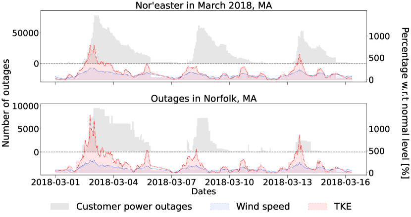
Figure 1: The number of outaged customers and the meteorological factors, including wind speed and turbulent kinetic energy.

A fundamental challenge in strengthening power system resilience lies in the immense difficulty of restoring electricity after a severe event has caused widespread damage. The recent Los Angeles wildfires highlight how extreme winds can overwhelm firefighting efforts, making containment impossible even with abundant resources, let alone the rapidly repairing damaged transmission lines [5]. The aftermath of major storms presents similar challenges – damaged infrastructure can take weeks or even months to restore, leading to severe economic and social repercussions. However, the impact of such events can be significantly mitigated, and in some cases, entirely avoided through proactive resilience planning. For example, preemptive de-energization strategies have been successfully implemented in California to reduce wildfire risks [6], while grid hardening and strategic upgrades have improved system resilience in hurricane-prone regions [7].

To proactively mitigate power grid disruptions, it is crucial to anticipate the long-term impact of extreme events on power systems and implement preemptive measures accordingly. Accurate forecasting enables utility companies and policymakers to assess risks, prioritize interventions, optimize grid reinforcement, and allocate resources efficiently. By identifying vulnerable regions in advance, decision-makers can develop strategies that not only reduce power disruptions but also strengthen overall grid resilience.

A widely used approach in such planning is the predict-then-optimize (PTO) framework, where forecasts inform downstream decisions [8]. However, conventional PTO approaches often fall short in high-stake decision making problems [9]. A high-quality forecast does not necessarily translate into effective decision-making, as small errors in predictive models can propagate into significant inefficiencies in downstream optimization tasks [10, 9]. This issue arises because conventional models are trained independently of decision-making objectives, meaning they may prioritize minimizing forecasting errors without considering how those errors impact critical decisions. As a result, even small deviations in predictions can lead to costly misallocations of resources, delayed responses, and suboptimal grid resilience strategies [11, 12]. Addressing this gap requires a more integrated approach that directly aligns predictive modeling with decision-making objectives, ensuring that forecasts are not only accurate but also actionable for proactive grid management.

This challenge becomes even more pronounced in system-wide decision-making, where resilience planning depends on aggregating independent predictions across multiple service units. Ensuring consistency across these independent predictions is inherently challenging, as errors in any individual unit’s forecast can propagate and compound, ultimately undermining the global decision quality. For instance, consider a utility company preparing for an approaching hurricane: if outage risks are underestimated in one region and overestimated in another, resources such as backup generators, repair crews, and grid reinforcements may be misallocated. Low-risk areas may be overprepared, while high-risk areas may lack sufficient resources, worsening service disruptions. These inconsistencies underscore the critical need for a holistic, system-wide approach that integrates predictions for multiple units with a global decision-making objective, ensuring coherent and globally optimized resilience strategies rather than fragmented, unit-specific responses.

To address the challenges of proactive resilience planning, we first propose a new decision-making paradigm, referred to as predict-all-then-optimize-globally (PATOG), which integrates predictive outage modeling across all service units with a global decision-making process for grid resilience enhancement. To solve PATOG problems, we then introduce a global-decision-focused (GDF) neural ordinary differential equation (ODE) model, which simultaneously predicts the long-term evolution of system functionality (quantified by the number of power outages) and optimizes global resilience decisions. Inspired by epidemiological models, our method conceptualizes power outage progression within each service unit as a dynamical system, where the failure and restoration processes evolve based on transmission line conditions, local weather, and socioeconomic factors. These transition dynamics are parameterized using neural networks, allowing the model to adapt to different hazard scenarios and geographic conditions. Instead of treating each service unit independently, our method holistically forecasts the outage evolution across the power grid and derives a globally coordinated intervention strategy. This enables utilities to allocate resources more effectively, mitigating service disruptions in a spatially and temporally coherent manner.

To assess our framework, we conduct experiments on both real-world and synthetic datasets. The real dataset captures outage events from a 2018 Nor’easter in Massachusetts, combining county-level outage reports [13] with meteorological data from NOAA’s HRRR model [14] and socioeconomic indicators from the U.S. Census Bureau [15] (Fig. 1). The synthetic dataset simulates real outage propagation using a simplified SIR model, enabling controlled evaluation under varying weather conditions and grid configurations. These datasets provide a robust testbed for assessing GDF in realistic resilience planning scenarios. Our results demonstrate significant improvements in forecast consistency, decision efficiency, and overall grid resilience, showcasing the potential of our approach to enable smarter, more proactive energy infrastructure management in the face of increasing hazard-induced disruptions.

We summarize our main contributions as follows:

• Propose a new predict-all-then-optimize-globally (PATOG) paradigm for system-wide decision-making problems in grid resilience management;

• Develop a novel method, referred to as global-decision-focused (GDF) neural ODEs, for solving PATOG problems;

• Demonstrate that GDF neural ODEs outperform baseline methods across multiple grid resilience management tasks through experiments on synthetic data.

• Evaluate our approach on a unique real-world customer-level outage dataset, uncovering key insights that inform more effective grid resilience strategies.

I-A Related Work

This section reviews key advancements in outage modeling, decision-focused learning (DFL), and grid operation optimization, with an emphasis on their practical applications in power system resilience. Despite significant progress, existing methods separate forecasting from optimization, causing inefficiencies in decision-making. This review underscores the need for a unified framework that aligns predictive models with resilience objectives to enhance grid reliability in extreme natural hazards.

Grid Operation Optimization. Grid optimization has been widely studied to improve power system resilience, covering areas such as distributed generator (DG) placement [16, 17, 18], infrastructure reinforcement [19], and dynamic power scheduling [20, 21]. However, traditional approaches often follow a two-stage predict-and-mitigate paradigm—first forecasting system conditions and then optimizing responses [22]. This disconnect between prediction and optimization results in suboptimal grid operations, particularly under high uncertainty, where even small forecasting errors can cause significant deviations from the optimal response [12, 11].

Two critical problems in this domain illustrate the limitations of such approach. The generator deployment problem determines optimal DG placement and sizing to mitigate outages caused by extreme events [17, 18, 16]. Traditional approaches emphasize on optimization techniques like genetic algorithms and particle swarm optimization to minimize power losses and improve voltage stability [18]. Similarly, the power line undergrounding problem aims to reinforce the grid infrastructure by undergrounding transmission lines to withstand hazards such as hurricanes and earthquakes [23, 24]. Conventional methods prioritize static risk assessments using historical data, lacking adaptability to evolving threats [25, 26]. While these approaches improve resilience, they fail to account for dynamic outage scenarios, limiting their effectiveness in extreme events.

To address these limitations, this paper proposes integrating decision-focused learning (DFL) with predictive modeling. By embedding decision-making objectives directly into the learning process, our approach aligns predictions with optimization goals, improving resource allocation and grid reinforcement strategies. This integrated approach enables more adaptive and proactive decision-making, enhancing grid resilience against escalating natural-hazard-related risks.

Power Outage Modeling. Accurate power outage forecasting is crucial for enhancing grid reliability and resilience [27, 28]. Various machine learning and statistical methods have been employed to predict outages under different conditions. For example, some studies have focused on forecasting outage durations using historical natural language processing (NLP) data [29]. These approaches incorporate neural networks enriched with environmental factors and semantic analysis of field reports, providing real-time updates and enhancing predictive performance through text analysis.

Additionally, ordinary differential equations have been widely used to model dynamic systems, such as outage propagation, capturing evolving disruptions under various conditions [30, 31]. For instance, adaptations of the Susceptible-Infected-Recovered (SIR) model from epidemiology have been applied to simulate outage propagation, drawing parallels between power failures and disease spread [32].

While these models provide valuable insights, they often lack the granularity needed for city- or county-level decision-making, limiting their practical application to localized resilience planning. By integrating local weather forecasts and socio-economic data into compartmental neural ODE models, our approach offers forecasting of local outage dynamics, enabling more targeted and effective interventions.

Decision-Focused Learning. Decision-focused learning (DFL) integrates predictive machine learning models with optimization, aligning training objectives with decision-making rather than purely maximizing predictive accuracy. Unlike traditional two-stage approaches, where predictions are first generated and then used as inputs for optimization, DFL enables end-to-end learning by backpropagating gradients through the optimization process. This is achieved via implicit differentiation of optimality conditions such as KKT constraints [33, 34] or fixed-point methods [35, 36]. For nondifferentiable optimizations, approximation techniques such as surrogate loss functions [8], finite differences [37], and noise perturbations [38] have been developed. Recent work has also explored integrating differential equation constraints directly into optimization models, enabling end-to-end gradient-based learning while ensuring compliance with system dynamic constraints [39, 40].

A well-studied class of DFL problems involves linear programs (LPs), where the Smart Predict-and-Optimize (SPO) framework [8] introduced a convex upper bound for gradient estimation, enabling cost-sensitive learning for optimization. Subsequent work has extended DFL to combinatorial settings, including mixed-integer programs (MIPs), using LP relaxations [41, 42]. Recent advances, such as decision-focused generative learning (Gen-DFL) [43], tackle the challenge of applying DFL in high-dimensional setting by using generative models to adaptively model uncertainty.

Differentiable Optimization. A key enabler of DFL is differentiable optimization (DO), which facilitates gradient propagation through differentiable optimization problems, aligning predictive models with decision-making objectives [44]. Recent advances extend DO to distributionally robust optimization (DRO) for handling uncertainty in worst-case scenarios, improving decision quality under data scarcity [45, 46]. Beyond predictive modeling, DO has advanced combinatorial and nonlinear optimization through implicit differentiation of KKT conditions [33], fixed-point methods [35], and gradient approximations via noise perturbation [38] and smoothing [37]. These techniques bridge forecasting with optimization, ensuring decision-aware learning. In this work, DO enables the backpropagation of resilience strategy losses, aligning the spatio-temporal outage prediction model with grid optimization objectives.

II Predict All Then Optimize Globally

In this section, we first provide an overview of decision-focused learning (DFL) and its application to solving predict-then-optimize (PTO) problems. We then introduce a new class of decision-making problems termed predict-all-then-optimize-globally (PATOG). Unlike traditional PTO approaches, which generate instantaneous or overly aggregated forecasts and optimize decisions independently, PATOG explicitly accounts for how predictions evolve over time and space, integrating them into a single, system-wide optimization framework.

PATOG is particularly useful for grid resilience management, where decisions must consider complex interactions across all service units. A key example is the mobile generator distribution problem. In a conventional PTO setting, potential damage from an extreme weather event is first forecasted for each unit independently. Decisions, such as scheduling power generator deployments, are then made in isolation, without considering the evolving conditions of other units. This localized approach often leads to resource misallocation and suboptimal resilience outcomes. In contrast, PATOG embeds these interdependencies into a global optimization problem, enabling system-wide decision-making that improves predictive models by incorporating cross-unit interactions. This results in more robust and effective resilience planning.

II-A Preliminaries: Decision-Focused Learning

The predict-then-optimize (PTO) has been extensively studied across a wide range of applications [22, 9]. It follows a two-step process: First, predicting the unknown parameters $\mathbf{c}$ using a model $f_{\theta}$ based on the input $\bm{z}$, denoted as $\hat{\bm{c}}\coloneqq f_{\theta}(\bm{z})$. Second, solving an optimization problem:

$$\bm{x}^{*}(\hat{\mathbf{c}})=\arg\min_{\bm{x}}g(\bm{x},\hat{\mathbf{c}}),$$ (1)

where $g$ is the objective function and $\bm{x}^{*}(\hat{\mathbf{c}})$ represents the optimal decision given the predicted parameters. This framework has numerous practical applications in power grid operations. For example, PTO is used in power grid operations to predict system stress using synchrophasor data, optimize outage management by forecasting disruptions and proactively dispatching restoration crews, and enhance renewable integration by predicting fluctuations in wind and solar generation to improve scheduling and grid balancing [22]. These predictive insights enable system operators to make informed strategic decisions, enhancing grid reliability and resilience.

However, the conventional two-stage approach does not always lead to high-quality decisions. In this approach, the model parameter $\theta$ is first trained to minimize a predictive loss, such as mean squared error. Then the predicted parameters $\hat{\mathbf{c}}$ are used to solve the downstream optimization. This separation between prediction and optimization can result in suboptimal decisions, as the prediction model is not directly optimized for decision quality [47].

To address this limitation, the decision-focused learning (DFL) integrates prediction with the downstream optimization process [9]. Instead of optimizing for predictive accuracy, DFL trains the model parameter $\theta$ by directly minimizing the decision regret [9]:

$$\theta^{*}=\arg\min_{\theta}\mathbb{E}\left[g(\bm{x}^{*}(f_{\theta}(\bm{z})),\mathbf{c})-g(\bm{x}^{*}(\mathbf{c}),\mathbf{c})\right].$$

This approach ensures that the model is learned with the ultimate goal of improving decision quality, making it particularly effective for PTO problems. Note that we assume that the constraints on decision variable $\bm{x}$ are fully known and do not depend on the uncertain parameters $\mathbf{c}$ in this study. This assumption simplifies the problem by ensuring that all feasible solutions $\bm{x}$ remain valid regardless of the parameter estimates.

II-B Proposed PATOG Framework

The objective of PATOG in this work is to develop proactive global recourse actions that enable system operators to better prepare for natural hazards. These actions may include preemptive dispatch of mobile generators, strategic load shedding, grid reconfiguration, or reinforcement of critical infrastructure. The PATOG consists of two steps: ($i$) Predicting the temporal evolution of unit functionality across all the service units in the network throughout the duration of a hazard event. ($ii$) Deriving system-wide strategies that minimize overall loss based on all the predictions, enabling optimized resource allocation by anticipating critical failures before they occur.

Consider a power network consisting of $K$ geographical units, where each unit $k$ serves $N_{k}$ customers. We define the global recourse actions as $\bm{x}\coloneqq\{x_{k}\}_{k=1}^{K}$, where $x_{k}$ represents the action taken for unit $k$. A key challenge in designing effective actions is understanding how the system will respond to an impending hazard event. To this end, we use the number of customer power outages, which is publicly accessible via utility websites, as a measure of system functionality [22].

To model the outage dynamics, we represent the outage state of each unit $k$ using a dynamical system over the time horizon $[0,T]$ during a hazard event. During the event, the state of each unit $k$ at time $t$ is represented by three quantities:

• $Y_{k}(t)\in\mathbb{Z}_{*}$: the number of customers experiencing outages;

• $U_{k}(t)\in\mathbb{Z}_{*}$: the number of unaffected customers;

• $R_{k}(t)\in\mathbb{Z}_{*}$: the number of recovered customers.

The total number of customers, $N_{k}$, in the unit $k$ remains constant throughout the event, satisfying the following constraint:

$$Y_{k}(t)+U_{k}(t)+R_{k}(t)=N_{k},~\forall t\in[0,T].$$

For compact representation, we define the state vector for unit $k$ as $\mathbf{S}_{k}(t)\coloneqq[U_{k}(t),R_{k}(t),Y_{k}(t)]^{\top}$. To simplify notation, we collectively represent the outage states across all units over the time horizon as $\mathbf{S}\coloneqq\{\mathbf{S}_{k}(t)\mid t\in[0,T]\}_{k=1}^{K}$.

Formally, we are tasked to search for the optimal action:

$$\bm{x}^{*}(\mathbf{S})= ~\arg\min_{\bm{x}}~g(\bm{x},\mathbf{S})$$ (2)

$$\text{s.t.}\quad\frac{\mathrm{d}\mathbf{S}_{k}(t)}{\mathrm{d}t}= ~f_{\theta}(\mathbf{S}_{k}(t),\bm{z}_{k}),~\forall k,$$ (3)

$$\mathbf{S}_{k}(0)= ~[N_{k},0,0]^{\top},~\forall k,$$ (4)

where $g$ quantifies the decision loss of the action $\bm{x}$ based on the predicted future evolution of outage states $\mathbf{S}$. The transition function $f_{\theta}$ models the progression of unaffected, recovered, and outaged customers in each unit over time, influenced by both local weather conditions and socioeconomic factors, jointly represented as covariates $\bm{z}_{k}\in\mathbb{R}^{p}$. We note that most power outages during extreme weather stem from localized transmission line damage, with cascading failures being rare [48, 49]. Thus, we assume each unit evolves independently under its local conditions.

We emphasize that (2) extends the traditional PTO framework by integrating predictions across multiple units over an extended future horizon to derive a single, globally optimized solution. Unlike PTO, which focuses only on instantaneous or localized dynamics, PATOG captures both temporal and spatial outage states while modeling how decisions influence outage dynamics across the entire system. This comprehensive approach enables proactive, system-wide high-resolution resilience strategies that adapt to evolving conditions.

III Global-Decision-Focused Neural ODEs

This section presents a novel decision-focused neural ordinary differential equations (ODE) model tailored for solving PATOG problems in grid resilience management. The proposed neural ODE model predicts outage progression at the unit level while simultaneously optimizing global operational decisions by learning model parameters in a decision-aware manner. We refer to this approach as global-decision-focused (GDF) Neural ODEs. Fig. 2 provides an overview of the proposed framework.

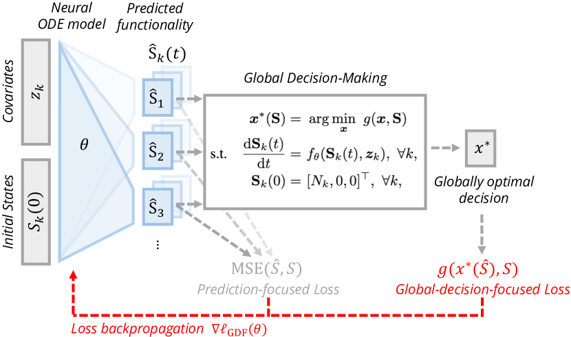
Figure 2: Overview of the proposed GDF framework. Given covariates $\bm{z}_{k}$ and initial states $\mathbf{S}_{k}(0)$ for all $K$ service units, a model parameterized by $\theta$ predicts the system states $\hat{\mathbf{S}}_{k}$ for all units. These predictions inform global decision-making, where optimal actions $\bm{x}^{*}(\hat{\mathbf{S}})$ minimize the global decision loss $g(\bm{x},\hat{\mathbf{S}})$. The framework optimizes $\theta$ by minimizing a global-decision-focused loss, regularized by a prediction-focused loss (e.g., MSE loss) to enhance predictive interpretability. Red arrows denote the backpropagation through $\nabla\ell_{\texttt{GDF}}(\theta)$, ensuring that the model learns both system-level decision quality and region-specific prediction accuracy.

III-A Neural ODEs for Power Outages

Assume that we have observations of $I$ natural hazards (e.g., hurricanes, and winter storms) in the history. For the $i$-th event, the observations in unit $k$ are represented by a data tuple, denoted by $(\bm{z}_{k}^{i},\{y_{k}^{i}(t)\})$, where $\bm{z}_{k}^{i}$ represents the covariates for unit $k$ during the $i$-th event and $y_{k}^{i}(t)$ is the number of customers experiencing power outages at time $t$. The outage trajectory $\{y_{k}^{i}(t)\mid t\in[0,T^{i}]\}$ is recorded at $15$-minute intervals. A significant challenge in modeling outage dynamics is the lack of detailed observations for the underlying failure and restoration processes. Specifically, while $y_{k}^{i}(t)$ provides the number of customers experiencing outages at time $t$, we do not directly observe the failure and restoration states, $U_{k}(t)$ and $R_{k}(t)$, respectively.

Drawing inspiration from the Susceptible Infectious Recovered (SIR) models commonly used in epidemic modeling [50], we conceptualize power outages within a unit as the spread of a “virus”. In this analogy, outages propagate among customers due to local transmission line failures, while restorations provide lasting resistance to subsequent outages. We formalize this analogy with the following two assumptions: ($i$) The number of unaffected customers $U_{k}(t)$ decreases over time as some customers transition from being unaffected to experiencing outages. This transition is governed by the failure transmission rate, denoted by $\phi(\bm{z}_{k};\theta_{U})$, which represents the probability of an outage per contact multiplied by the rate of such contacts, depending on its connectivity in the grid network. ($ii$) Conversely, the number of customers with restored power ($R_{k}(t)$) gradually increases as the system operator repairs transmission lines and restores service. This process is driven by the restoration rate, denoted $\phi(\bm{z}_{k};\theta_{R})$. Both transmission and restoration rates, $\phi(\bm{z}_{k};\theta_{U})$ and $\phi(\bm{z}_{k};\theta_{R})$, are functions of the local covariates $\bm{z}_{k}$, and are modeled using deep neural networks. Therefore, we model the outage state transition for each unit $k$ in (3), i.e., $\mathrm{d}\mathbf{S}_{k}(t)/\mathrm{d}t$, as follows:

$$\begin{cases}\begin{aligned} \mathrm{d}U_{k}(t)/\mathrm{d}t&=-\phi(\bm{z}_{k};\theta_{U})Y_{k}(t)U_{k}(t),\\ \mathrm{d}R_{k}(t)/\mathrm{d}t&=\phi(\bm{z}_{k};\theta_{R})Y_{k}(t),\\ \mathrm{d}Y_{k}(t)/\mathrm{d}t&=-\mathrm{d}U_{k}(t)/\mathrm{d}t-\mathrm{d}R_{k}(t)/\mathrm{d}t.\end{aligned}\end{cases}$$ (5)

These ODEs capture the dynamic evolution of power outage states within each unit $k$. For notational simplicity, we use $\theta\coloneqq\{\theta_{U},\theta_{R}\}$ to denote their parameters jointly.

In practice, we work with discrete observations $\{t_{j}\}_{j=0}^{T}$ and adopt the Euler method to approximate the solution to the ODE model [31], i.e.,

$$\mathbf{S}_{k}(t_{j+1})=\mathbf{S}_{k}(t_{j})+f_{\theta}(\mathbf{S}_{k}(t_{j}),\bm{z}_{k})\Delta t_{j},\quad\forall k,$$

where $\mathbf{S}_{k}(t_{j+1})$ and $\mathbf{S}_{k}(t_{j})$ are the history states at times $t_{j+1}$ and $t_{j}$, respectively, and $\Delta t_{j}\coloneqq t_{j+1}-t_{j}$ is time interval.

III-B Global-Decision-Focused Learning

The training loss for GDF Neural ODEs is formulated as the aggregated regret across all unit $k$, with an additional regularization term to ensure stability in prediction:

$$\ell_{\texttt{GDF}}(\theta)\coloneqq ~\frac{1}{I}\sum_{i}\left[g\Big{(}\bm{x}^{*}(\hat{\mathbf{S}}^{i}),{\mathbf{S}}^{i}\Big{)}-g\Big{(}\bm{x}^{*}({\mathbf{S}}^{i}),\mathbf{S}^{i}\Big{)}\right]+$$ (6)

$$~\lambda\cdot\frac{1}{IKT}\sum_{i,k,j}\left[y_{k}^{i}(t_{j})-\hat{Y}_{k}^{i}(t_{j})\right]^{2},$$

where ${\hat{\mathbf{S}}^{i}}$ is the predicted outages states across all units for event $i$.

The objective function (6) consists of two key components: ($i$) Global-decision-focused loss (first term): This term evaluates the quality of the optimal action based on predictions, capturing the impact of prediction errors on operational decisions. The loss and its gradient are computed over all geographical units affected by the event, ensuring that learning is guided by system-wide decision quality. However, this loss alone does not provide direct insights into the structure of outage trajectories, which may limit the interpretability of the learned model. ($ii$) Prediction-focused loss (second term): To address this limitation, a prediction-based penalty is introduced to minimize discrepancies between observed outage trajectories $y^{i}_{k}(t)$ and predicted values $\hat{Y}^{i}_{k}(t)$. This term refines the model’s ability to capture outage dynamics without explicitly observing the failure and restoration processes. A user-specified hyperparameter $\lambda$ governs the trade-off between prediction accuracy and the regret associated with suboptimal operational decisions.

The most salient feature of the proposed GDF neural ODEs method is its incorporation of both global and local perspectives. The global-decision-focused loss aggregates errors across all geographical regions and time steps, directly linking prediction quality to system-wide resilience measures and operational strategies (e.g., resource dispatch, outage management, and service restoration). Meanwhile, the prediction-focused component refines local accuracy by penalizing deviations at each service unit. By incorporating predictive regularization, the model empirically improves generalization to new events with unknown distributional shifts, mitigating overfitting, particularly given the limited availability of extreme event data.

III-C Model Estimation

The learning of GDF Neural ODEs is carried out through stochastic gradient descent, where the gradient is calculated using a novel algorithm based on differentiable optimization techniques [33, 44, 45]. To enable differentiation through the $\arg\min$ operator in (2) embedded in the global-decision-focused loss, we relax the decision variable $\bm{x}$ from a potentially discrete space to a continuous space. For combinatorial optimization problems, the problem is reformulated as a differentiable quadratic program, and a small quadratic regularization term is added to ensure continuity and strong convexity [42]. Formally, we replace the original objective in (2) with the following:

$$\min_{\bm{x}}g(\bm{x},\mathbf{S})+\rho\|\bm{x}\|_{2}^{2},$$ (7)

where $\rho>0$ ensures differentiability. More implementation details can be found in Appendix -D.

Algorithm 1 Learning of GDF Neural ODEs

Input: Data $\mathcal{D}=\{(\bm{z}_{k}^{i},\{y_{k}^{i}(t)\})\}$, initial parameter $\theta_{0}$, initial states $\mathbf{S}^{i}(0)$, learning rate $\eta$, trade-off parameter $\lambda$, epochs $N$.
Output: $\theta^{*}$

1: for epoch $n=1,\dots,N$ do

2:  for $i=1$ to $I$ do

3:   Initialize: $\hat{\mathbf{S}}^{i}(0)\leftarrow\mathbf{S}^{i}(0)$.

4:   for $j=1$ to $T_{i}$ do

5:    $\hat{\mathbf{S}}^{i}(t_{j})\leftarrow\hat{\mathbf{S}}^{i}(t_{j-1})+f_{\theta}(\hat{\mathbf{S}}^{i}(t_{j-1}),\bm{z}_{k}^{i})\Delta t_{j-1}$

6:   end for

7:   $\ell_{\texttt{GDF}}^{i}(\theta)\leftarrow g\big{(}\bm{x}^{*}(\hat{\mathbf{S}}^{i}),\mathbf{S}^{i}\big{)}-g\big{(}\bm{x}^{*}(\mathbf{S}^{i}),\mathbf{S}^{i}\big{)}$

8:   $\theta\leftarrow\theta-\eta\,\nabla_{\theta}\ell_{\texttt{GDF}}^{i}(\theta)$.

9:  end for

10:  for each mini-batch $\mathcal{B}\subset\mathcal{D}$ do

11:   $\ell_{\text{Pred}}(\theta)\leftarrow\frac{1}{|\mathcal{B}|KT}\sum_{(i,k,t)\in\mathcal{B}}\Big{[}y_{k}^{i}(t)-\hat{Y}_{k}^{i}(t)\Big{]}^{2}$

12:   $\theta\leftarrow\theta-\eta\,\lambda\,\nabla_{\theta}\ell_{\text{Pred}}(\theta)$.

13:  end for

14: end for

15: return  $\theta$

IV Application: Mobile Generator Deployment

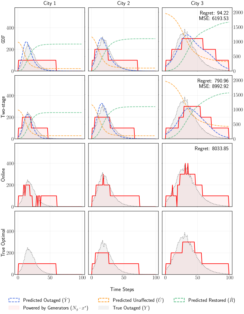
Figure 3: A synthetic example of the mobile generator deployment problem for a system with three cities and five generators ($Q_{w}=5$). The $y$-axis represents the number of outaged households. In this example, the transportation cost is set to $c=1000$, the customer interruption cost is $\tau=50$, and the operational cost is $\gamma=0.2$. Four methods are compared on out‑of‑sample data: the proposed GDF framework (regret = $94.22$), a two‑stage approach (regret = $8992.92$), an online baseline (regret = $790.96$), and the optimal solution with the lowest total cost (regret = $8033.85$). Details of the synthetic data setup are provided in Section V-A.

Our method is broadly applicable to various proactive decision-making problems in grid operations, particularly in response to potential hazard events. This section highlights the adaptability of GDF by applying it to a mobile generator deployment task [16, 17, 18], a representative PATOG problem.

The objective of the mobile generator deployment problem is to strategically deploy mobile (e.g., diesel) generators across a network of potentially affected sites before a large-scale power outage to minimize associated costs. Due to the time-sensitive nature of power restoration, it is crucial to anticipate the spatiotemporal dynamics of outages while accounting for operational constraints such as generator capacity, fuel availability, and transportation logistics. GDF is well-suited for this task as it jointly learns outage patterns across cities over the planning horizon while optimizing deployment decisions, enabling proactive decision-making that adapts to evolving conditions.

Formally, let $Q_{w}\in\mathbb{Z}_{+}$ denote the initial inventory of generators at warehouse $w$. For simplicity, we assume that warehouses also function as staging areas, where generators are initially stored and returned after deployment. We assume that each generator has a fixed maximum capacity, capable of supplying electricity to $N_{g}$ customers, and that a single extreme event is anticipated. The planning horizon is discretized into uniform time periods $\mathcal{T}=\{1,2,\dots,T\}$, where ${T}$ represents the expected duration of the outage. Let $\mathcal{K}=\{1,2,\dots,K\}$ be the set of $K$ service units (e.g., cities or counties) where generators can be deployed, and $\mathcal{W}=\{1,\dots,W\}$ be the set of warehouses where all generators are initially stored. We denote the stock of generators in unit $k$ at time $t$ as $q_{tk}$.

The mobile generator deployment problem is therefore defined on a directed graph denoted by $(\mathcal{V},\mathcal{E})$, where $\mathcal{V}\coloneqq\mathcal{K}\cup\mathcal{W}$ is the vertex set, and $\mathcal{E}$ represents the edge set defining feasible transportation routes. Each edge $(k,k^{\prime})\in\mathcal{E}$ incurs a transportation cost $c_{kk^{\prime}}$. The decision variables, ${\bm{x}=\{x_{tkk^{\prime}}\}}$, $(k,k^{\prime})\in\mathcal{E}$, $t\in\mathcal{T}$, specifies the transportation schedule, where $x_{tkk^{\prime}}\in\mathbb{Z}_{+}$ represents the number of generators transported from location $k$ to $k^{\prime}$ at time $t$. For simplicity, we assume negligible travel and deployment time, allowing generators to become operational immediately upon arrival to supply power to $N_{g}$ customers.

The cost function of generator deployment problem is:

$$g(\bm{x},\mathbf{S})\coloneqq$$ (8)

$$\underbrace{\sum_{(k,k^{\prime})\in\mathcal{E}}\sum_{t=1}^{T}c_{kk^{\prime}}x_{tkk^{\prime}}}_{\text{Transportation Cost}}+\underbrace{\gamma\sum_{k\in\mathcal{K}}\sum_{t=1}^{T}q_{tk}\vphantom{\sum_{(k,k^{\prime})\in\mathcal{E}}\sum_{t=1}^{T}c_{kk^{\prime}}x_{tkk^{\prime}}}}_{\text{Operation Cost}}+\underbrace{h(\bm{x},\mathbf{S})\vphantom{\sum_{(k,k^{\prime})\in\mathcal{E}}\sum_{t=1}^{T}c_{kk^{\prime}}x_{tkk^{\prime}}+\gamma\sum_{k\in\mathcal{K}}\sum_{t=1}^{T}q_{tk}}}_{\text{Outage Cost}},$$

which consists of three components: ($i$) Transportation Cost: The cost of delivering generators from warehouses to service units. ($ii$) Operation Cost: The fixed operational cost per unit time ($\gamma$) for deployed generators. ($iii$) Outage Cost: Economic loss due to power outages, determined by the number of customers experiencing outages given the generator deployment decision $\bm{x}$. For simplicity, we define the outage cost as:

$$h(\bm{x},\mathbf{S})=\tau\sum_{k\in\mathcal{K},t\in\mathcal{T}}\max\Big{\{}Y_{k}(t)-q_{tk}N_{g},0\Big{\}},$$

where $\tau$ denotes unit customer interruption cost, an adapted version of the Value of Lost Load (VoLL) [51], representing the economic impact per household outage per day, and $Y_{k}(t)$ denotes the number of outages in service unit $k$ at time $t$, extracted from the state $\mathbf{S}$ according to (5). This framework primarily evaluates system functionality based on the number of customers experiencing outages ($Y$). It is worth emphasizing that it is flexible to incorporate additional metrics, including the number of recovered customers ($R$) and unaffected customers ($U$), if needed.

The transportation and inventory constraints of the mobile genereator deployment are as follows:

$$q_{0k}=0,\quad\forall k\in\mathcal{K}$$ (9)

$$q_{0w}=Q_{w},\quad\forall w\in\mathcal{W}$$ (10)

$$q_{tk}=\sum_{t}(\sum_{k^{\prime}\in\mathcal{K}}x_{tk^{\prime}k}-\sum_{k^{\prime}\in\mathcal{K}}x_{tkk^{\prime}}),\quad\forall k\in\mathcal{V}$$ (11)

$$x_{tkk^{\prime}}\leq C,\quad\forall t\in\mathcal{T},(k,k^{\prime})\in\mathcal{E}$$ (12)

$$\sum_{k\in\mathcal{V}/{\{k^{\prime}\}},t\in\mathcal{T}}x_{tkk^{\prime}}=\sum_{k\in\mathcal{V}/{\{k^{\prime}\}},t\in\mathcal{T}}x_{tk^{\prime}k},\quad\forall k^{\prime}\in\mathcal{V},$$ (13)

$$q_{kk^{\prime}},x_{tkk^{\prime}}\in\mathbb{Z}_{+},\,\quad\forall(k,k^{\prime})\in\mathcal{E},\,\forall t\in\mathcal{T}.$$ (14)

Constraints (9) and (10) establish the initial generator stock at each location. Equation (11) keeps track of the generator stock in each unit. Inequality constraint (12) limits the flow between service units or warehouses in $\mathcal{E}$ to a maximum capacity $C$. Finally, equation (13) ensures flow conservation, requiring that the total inflow of generators equals the total outflow over the planning horizon for each node in the network. As a result, all generators return to the staging areas after the events.

To implement the deployment strategy based on our GDF framework, we first predict outage levels $\hat{Y}_{k}(t)$ for all service units using the neural ODE model specified in (5). The model is learned by minimizing the GDF loss in (6). These global-deision-focused predictions are then integrated into the objective function (8) of the mobile generator deployment problem, and the decisions are derived by solving a mixed-integer linear programming (MILP). Figure 3 illustrates the performance of GDF in a stylized mobile generator deployment problem. As shown, GDF significantly reduces regret compared to two-stage and online baselines. The online algorithm takes a reactive approach, frequently relocating generators and incurring high operational costs, while the two-stage method fails to capture system-wide dynamics, leading to suboptimal decisions. In contrast, GDF’s globally optimized approach ensures more effective and cost-efficient resource allocation, enhancing overall grid resilience with minimal cost.

V Experiments

In this section, we evaluate the proposed GDF on two grid resilience management problems—mobile generator deployment and power line undergrounding. The numerical results demonstrate its superior performance compared to conventional two-stage methods, enabling better decision-making in the face of natural hazards.

V-A Dataset Overview

We evaluate GDF using both real and synthetic datasets to assess its effectiveness in outage prediction and resilience planning. The real dataset records the number of customers affected by outages during the 2018 Nor’easter in Massachusetts [52], while the synthetic outage trajectories are generated using a simplified SIR model.

V-A1 Real Dataset

The real dataset used in this study comprises county-level customer outage counts [13], combined with meteorological measurements and socioeconomic indicators from regions affected by a Nor’easter snowfall event in Massachusetts in 2018 (Fig. 1). Meteorological variables—such as wind speed, temperature, and pressure—are sourced from NOAA’s High-Resolution Rapid Refresh (HRRR) model [14]. Socioeconomic and demographic data are collected from the U.S. Census Bureau’s American Community Survey [15] and include median household income, median age, the number of food stamp recipients, the unemployment rate, the poverty rate, college enrollment, mean travel time to work, and average household size. These variables capture economic and mobility factors that may influence outage recovery dynamics and the effectiveness of emergency response efforts.

A key advantage of using outage data from Massachusetts during the 2018 Nor’easter event [52] is that three consecutive snowstorms impacted the power system within a short 15-day period, during which the local infrastructure remained largely unchanged. This allows us to reasonably assume that the outage patterns from these storms follow the same underlying data distribution, making them suitable for widely used train-test evaluation. Accordingly, we use the first storm for training and the second for testing the effects of different frameworks, while excluding the third storm due to its relatively minor impact. Fig. 1 illustrates the spatiotemporal dynamics of the real dataset.

V-A2 Synthetic Dataset

To augment these real-world observations and enable experiments under varying conditions, synthetic outage trajectories are generated using a simplified SIR model. In this model, each county is treated as an independent population that experiences outages and eventually recovers, in accordance with the dynamics specified in (5). Simulated weather conditions are incorporated to modulate the transmission rate, thereby capturing the variability and severity of extreme events. This synthetic dataset provides a realistic and flexible testbed for systematically evaluating the proposed decision-focused learning framework under different scenarios.

V-B Experimental Setup

To evaluate the effectiveness of the proposed Global Decision-Focused (GDF) Neural ODE framework, we conduct experiments on two application domains: power line undergrounding and mobile generator deployment as introduced in Section IV. For both problems, predictions for the entire time horizon are made before the occurrence of the hazard, reflecting the practical challenge of collecting data in real time during a developing hazard [53]. Consequently, for both problems, when the hazard surpasses a predefined threshold (1% in our experiments), the ODE model’s initial conditions are set, and decisions are made accordingly.

In the generator deployment problem, we assume a single centralized warehouse as the sole source of generators, with no inter-county transfers. Generators are dispatched from the warehouse to affected counties and must eventually return for refueling, following the framework described in Section V-C1. The online baseline method assumes a one-day lag, making greedy decisions based on data from the previous day, reflecting a realistic delay in data availability for decision-makers without predictive insights. We also report results for different lag values, while all online methods reported in the plots use a fixed lag of one day.

The training process consists of two stages. Initially, the neural ODE model is trained using a standard mean squared error (MSE) loss, providing a predictive model baseline. Optimal decisions based on these baseline predictions serve as a two-stage reference. In the second stage, the baseline model is then used to initialize end-to-end training with the combined loss function in (6), which integrates both decision-focused and prediction-focused objectives, as described in Algorithm 1.

We compare the proposed model, GDF, with spatio-temporal neural ODE models trained solely on MSE loss (Two-stage) and the ground truth optimal decision baseline (True Optimal). We also include results from an online method for the mobile generator deployment problem. Evaluation is based on three metrics: ($i$) prediction accuracy, measured as the mean squared error between predicted and observed outages; ($ii$) decision loss, represented by the total cost for generator deployment or the total System Average Interruption Duration Index (SAIDI) for grid hardening; and ($iii$) regret, defined as the cost difference between the ground truth optimal decision and the decision based on the model’s predictions. For all experiments on synthetic datasets, reported results and standard deviations are calculated with three different random seeds, which generate varying outage curves and weather conditions.

TABLE I: Out-of-Sample Performance for Generator Distribution problem (Synthetic Data). Results are averaged over 3 repeated experiments with standard error (SE) in the brackets.

Model	Transportation Cost = 100			Transportation Cost = 500			Transportation Cost = 1000
	MSE	Cost	Regret	MSE	Cost	Regret	MSE	Cost	Regret
Ground Truth	/	6515.6 (74.4)	0	/	11271	0	/	16271	0
Online (lag = 1)	/	8163.7 (293.4)	1648.1 (358.6)	/	19630.4 (1514.8)	8358.7 (1576.8)	/	33963.7 (3042.2)	17692.1 (3104.4)
Online (lag = 3)	/	8978.6 (277.6)	2462.9 (313.8)	/	22045.2 (1493.3)	10773.6 (1522.9)	/	38378.6 (3020.2)	22106.9 (3050.4)
Online (lag = 5)	/	9618.9 (57.3)	4939.9 (111.1)	/	22152.2 (498.5)	16497.9 (557.8)	/	37818.9 (1074.7)	32164.5 (1135.0)
Two-stage	9336.0 (975.6)	6671.5 (4328.7)	155.8 (33.3)	9336.0 (975.6)	11465.8 (94.6)	194.2 (107.3)	9336.0 (975.6)	16517.8 (133.9)	246.1 (112.7)
GDF	9709.6 (3055.6)	6668.7 (4365.9)	153.0 (19.8)	8671.2 (1553.7)	11428.1 (87.1)	156.4 (44.2)	6981.1 (1874.0)	16395.9 (89.0)	124.2 (36.3)

TABLE II: Out-of-Sample Performance of Power Line Undergrounding Problem with Real and Synthetic Data

Models	Nor’easter, MA, 2018			Synthetic
	MSE ($\times 10^{3})$	SAIDI	Regret	MSE ($\times 10^{3})$	SAIDI	Regret
True Optimal	/	218.2	/	/	15.6	/
Two-stage	117.4	328.3	112.1	13.5	16.1	0.5
GDF	165.6	312.7	94.5	13.1	15.6	0

Figure 4: Performance Comparison for Synthetic Mobile Generator Deployment: A detailed comparison of regret outcomes for GDF, Two-Stage, and Online methods under varying customer interruption costs ($\tau$), transportation cost factors ($c$), operational costs ($\gamma$), and numbers of generators ($Q_{w}$).

V-C Results

This section presents the results of GDF on mobile generator deployment and power line undergrounding, evaluated in terms of predictive accuracy and decision quality. Results on both synthetic and real datasets demonstrate that GDF improves decision-making compared to conventional two-stage methods, enabling a more effective response to natural hazards.

V-C1 Mobile Generator Deployment Problem

Table I summarizes the out-of-sample performance for the generator deployment problem on synthetic data across three transportation cost factors (100, 500, and 1000). As the transportation cost increases, the improvement in decision quality for GDF compared to the Two-stage approach becomes more apparent. This highlights the importance of scheduling and proactive actions when transportation costs are high, demonstrating the clear advantage of GDF.

To understand how GDF impacts MSE-trained predictive models, see Fig.3. By slightly increasing the predicted outage for city 3, GDF proactively allocated more resources to city 3’s anticipated outage, drawing from the stock allocated to city 1. In contrast, the Two-stage method did not make this adjustment. While this change in prediction is subtle, it results in significantly lower regret. Remarkably, the GDF model achieves an MSE comparable to or better than that of the MSE-trained model in TableI, albeit with higher variance. This shows that improved decision quality was not achieved at the expense of predictive accuracy, but rather through targeted and meaningful adjustments in prediction.

We conducted extensive experiments on synthetic data for the mobile generator deployment problem under various settings, as shown in Fig. 4. The decision quality improvement of GDF relative to the Two-stage method initially increases with transportation cost before eventually declining. This behavior is expected: higher transportation costs highlight the importance of proactive actions. However, when transportation costs become so high that the best strategy is effectively to remain idle, the potential savings for proactive actions diminish. Similarly, we observed that as operational costs and available generators increase, the performance gap between GDF and the other two methods narrows.

V-C2 Power Line Undergrounding

Table II presents the out-of-sample performance on both the Nor’easter, MA, 2018 event and the synthetic dataset. For the real dataset, the proposed GDF model—despite a slightly higher MSE—delivers improved decision quality, achieving a lower SAIDI and reduced regret compared to the Two-stage baseline. On the synthetic dataset, GDF similarly outperforms the Two-stage method in decision quality while maintaining a low MSE, possibly due to the relatively simple prediction tasks. These results confirm that GDF leads to better overall decision performance in real and synthetic settings.

Overall, the experimental results on both real and synthetic data demonstrate that GDF achieves substantial improvements in decision quality compared to the traditional Two-stage approach. Although both models exhibit comparable prediction accuracy, GDF consistently yields lower regret values, highlighting the benefits of proactive scheduling and decision-focused training.

VI Conclusion

This paper presented a novel framework for grid resilience management that jointly optimized prediction accuracy and global decision quality. Experimental results on both real and synthetic datasets demonstrated that, while achieving comparable MSE results to the conventional two-stage approach, GDF consistently yielded lower regret and better decisions. These findings suggest that integrating decision-focused learning enhances proactive scheduling and resource allocation, enabling system operators to more effectively mitigate outages. Future work will explore integrating real-time data streams to improve responsiveness, incorporating renewable energy forecasting, and adapting the framework to larger network systems.

-A Ablation Study

To evaluate the impact of the prediction error weight $\lambda$ in (6) on balancing prediction accuracy and decision quality, we conducted an ablation study with various $\lambda$ values on synthetic dataset. Results in Table III indicate that a lower $\lambda$ shifts the model’s focus toward decision quality, reducing decision regret by aligning predictions with resilience goals, albeit with a slight trade-off in MSE, compared to two-stage method. We note that such a design offers better flexibility and interpretability for the GDF-trained decision-making models.

TABLE III: Effect of $\lambda$ on Mobile Generator Deployment Problem.

Metric	$\lambda$			Baselines
	0	1	10	Two-stage	Online
MSE ($\times 10^{3}$)	9.7	9.5	9.6	9.3	/
Cost	6668.7	6609.5	6611.8	6631.7	8163.7
Regret	153.0	135.7	138.0	155.8	1648.1

-B Detailed Description on Online Algorithms for Mobile Generator Deployment Problem

We include pesudocode for the proposed online baseline allocation methods in Alg. 2.

Algorithm 2 Observe-then-optimize algorithm for mobile generator deployment problem

Input: Observations or forecasts $Y_{t,i}$, parameters $(\tau,\,N_{g},\,\gamma)$, warehouse stock $s_{w}$, etc.
Output: Shipping decisions $\{x^{\text{to}}_{t,i},x^{\text{back}}_{t,i}\}$ for each time $t$ and city $i$.

1: for $t=1$ to $T$ do

2:  — update warehouse and city stocks from previous shipments —

3:  for each city $i$ do

4:   Compute demand shortfall $d_{t,i}\leftarrow\max(0,\ \lceil Y_{t,i}/N_{H}\rceil-q_{t,i})$.

5:   $x^{\text{to}}_{t,i}\leftarrow\min(s_{w}(t),\,d_{t,i})$  // send enough to cover shortfall

6:   $x^{\text{back}}_{t,i}\leftarrow 0$  // no return shipments

7:  end for

8: end for

-C Power Line Undergrounding

Power line undergrounding is a grid-hardening measure against extreme meteorological events (such as hurricanes and heavy snowfalls) [23, 24, 25, 26]. Although effective, it involves substantial costs for the authority and causes significant disruptions to local communities [54, 55]. The objective of the power line undergrounding problem is to select an optimal subset of locations for underground interventions under budget constraints [24, 25, 26], in anticipation of an incoming hazard.

To formalize the decision-making problem, let $x_{k}$ be a binary variable indicating whether city $k$ is selected for undergrounding. With $K$ cities in total, the decision vector is $\bm{x}=[x_{1},\dots,x_{K}]^{\top}$, and $\hat{\mathbf{S}}$ denotes the predicted outage states. We then define:

$$\min_{\bm{x}} g(\bm{x},\hat{\mathbf{S}}),$$ (15)

s.t. $$\sum_{k=1}^{K}x_{k}\,\leq\,C,$$

$$x_{k}\,\in\,\{0,1\},\quad k=1,\dots,K,$$

where $g(\bm{x},\hat{\mathbf{S}})$ is the decision loss that quantifies the impact of outages given the chosen undergrounding plan $\bm{x}$.

We adopt the System Average Interruption Duration Index (SAIDI) [56] to measure how outages affect the population. Let $Y_{k}(t)$ be the (true) number of outages at city $k$ and time $t$, and $N_{k}$ be the total number of customers in city $k$. Since undergrounding is assumed fully effective, a city $k$ with $x_{k}=1$ incurs no further outages from the event. Hence, the decision loss is:

$$g(\bm{x},\mathbf{S})\;=\;\frac{1}{K}\,\sum_{k=1}^{K}\frac{1}{N_{k}}\int_{0}^{\infty}\Bigl{[}\bigl{(}1-x_{k}\bigr{)}\,Y_{k}(t)\Bigr{]}\,dt.$$ (16)

The optimal solution $\bm{x}^{*}$ to (15) is then the subset of cities to be undergrounded in order to minimize the total outage impact. Its performance is evaluated via $g(\bm{x}^{*},\mathbf{S})$ using true outage data $\mathbf{S}$.

-D Implementation Details of GDF

To get the gradient of (7), let matrix $H$ encode coefficients for all the linear constraints $\quad H\bm{x}\leq\bm{a}$, and ${\xi^{i}}$ represents a reformulation of the ground truth cost factors derived from $\mathbf{S}^{i}$, such that $g(\bm{x},\mathbf{S}^{i})={\xi^{i}}^{T}\bm{x}+\bm{b}$. Using the KKT conditions of the Lagrangian of the problem, the gradient of the QP in (7) is:

$$\nabla_{\theta}L_{\text{QP}}={\xi^{i}}^{T}K^{-1}\nabla_{\theta}\hat{\mathbf{S}}^{i},\quad K=\begin{bmatrix}2\rho_{x}I&H^{T}\\ H&0\end{bmatrix},$$ (17)

And $\nabla_{\beta,\gamma}\hat{\mathbf{S}}^{i}$ can obtained via backpropagation through the neural ODE model parameters $\{\theta_{U},\theta_{R}\}$ [31]. This gradient aims to improve decision quality across all cities and all events $i\in\{1,\dots,I\}$. Therefore, we refer to it as decision-focused gradient.

To be more specific about derivation of (17), the optimal solution $\bm{x}^{*}$ must satisfy the KKT conditions. We define the Lagrangian:

$$\mathcal{L}(\bm{x},\lambda)=g(\bm{x},\mathbf{S})+\rho\|\bm{x}\|_{2}^{2}+\lambda^{T}(H\bm{x}-\bm{a}).$$ (18)

The stationarity of $x^{*}$ for optimality gives:

$$\nabla_{x}g(\bm{x},\mathbf{S})+2\rho\bm{x}+H^{T}\lambda=0.$$ (19)

Since the optimal decision $\bm{x}^{*}$ satisfies the above KKT system, we can apply implicit differentiation. Taking the total derivative with respect to the predicted system state $\hat{\mathbf{S}}$:

$$\begin{bmatrix}\nabla^{2}_{xx}\mathcal{L}&H^{T}\\ H&0\end{bmatrix}\begin{bmatrix}\frac{d\bm{x}^{*}}{d\hat{\mathbf{S}}}\\ \frac{d\lambda}{d\hat{\mathbf{S}}}\end{bmatrix}=\begin{bmatrix}\frac{d(-\nabla_{x}g(\bm{x},\mathbf{S}))}{d\hat{\mathbf{S}}}\\ 0\end{bmatrix}.$$ (20)

where

$$\frac{d\bm{x}^{*}}{d\hat{\mathbf{S}}}=-K^{-1}\frac{d\nabla_{x}g}{d\hat{\mathbf{S}}},$$ (21)

and the KKT matrix $K$ is defined as:

$$K=\begin{bmatrix}2\rho I&H^{T}\\ H&0\end{bmatrix}.$$ (22)

since $\nabla^{2}_{xx}\mathcal{L}=2\rho I$ etc.

This allows us to compute the gradient of the loss function with respect to model parameters:

$$\nabla_{\theta}L_{\text{QP}}={\xi^{i}}^{T}K^{-1}\nabla_{\theta}\hat{\mathbf{S}}^{i}.$$ (23)

In practice, we regularize the GDF loss with prediction-focused gradient, as the prediction error is localized and requires fine-grained information for each individual sample unit. Specifically, we construct mini-batches $\mathcal{B}\subset\mathcal{D}$ from the training dataset $\mathcal{D}=\{\bm{z}_{k}^{i},y_{k}^{i}(t)\}$.

The neural ODE model generates forecasts $\hat{\mathbf{S}}_{\mathcal{B}}=f_{\beta,\gamma}(\bm{z}_{\mathcal{B}})$ for each sample in the batch. From these forecasts, we extract the predicted values $\hat{Y}_{\mathcal{B}}$, which are then used to compute the MSE loss:

$$L_{\text{MSE}}=\sum_{\mathcal{B}\subset\mathcal{D}}\frac{1}{|\mathcal{B}|}\sum_{(i,k,t)\in\mathcal{B}}\bigl{(}y_{k}^{i}(t)-\hat{Y}_{k}^{i}(t)\bigr{)}^{2}.$$ (24)

Finally, for each epoch, the model parameters $\theta$ is updated using a combination of both loss gradients, balanced by a hyperparameter $\lambda$:

$$\nabla_{\theta}L_{\text{total}}=\nabla_{\theta}L_{\text{GDF}}+\lambda\nabla_{\theta}L_{\text{MSE}}.$$ (25)

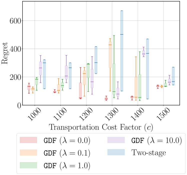
Figure 5: Regret performance of the GDF method with varying $\lambda$ values across different transportation cost factors in synthetic data for mobile generator deployment problem, benchmarked against the Two-stage approach.

-E Additional Results for the Mobile Generator Deployment Problem

This section presents supplementary results and visualizations for the mobile generator deployment problem.

As demonstrated in the ablation study, when $\lambda$ is large, the MSE dominates model training, reducing the advantage of GDF over MSE-trained models in decision quality. For more detailed ablation results, see Fig. 5, which shows that as $\lambda$ increases, the GDF results become similar to those of the two-stage method, resulting in larger regret and higher variance.

We also provide additional visualizations under varying conditions. In Fig. 6, we observe that when travel costs are low, the online strategy closely approximates the optimal strategy, resulting in small regret. This is because low travel costs allow the online method to frequently move generators based on previous day data at minimal expense, leading to near-optimal regret, whereas the two-stage and GDF methods rely more on predictions.

When comparing Fig.7 and Fig.8, we find that limited resources make the online strategy less effective than scenarios where resources are abundant. Without prepositioning based on prediction, the strategy must reposition the limited number of generators more frequently to respond to real-time outages, leading to higher transportation costs and, consequently, greater overall regret, compared to GDF and Two-stage methods.

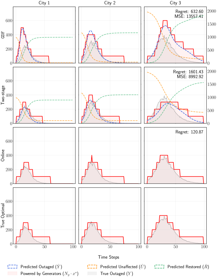
Figure 6: A synthetic example of the mobile generator deployment problem for a system with three cities and five generators ($Q_{w}=10$). The $y$-axis represents the number of outaged households. In this example, the transportation cost is set to $c=10$, the customer interruption cost is $\tau=1$, and the operational cost is $\gamma=2$.

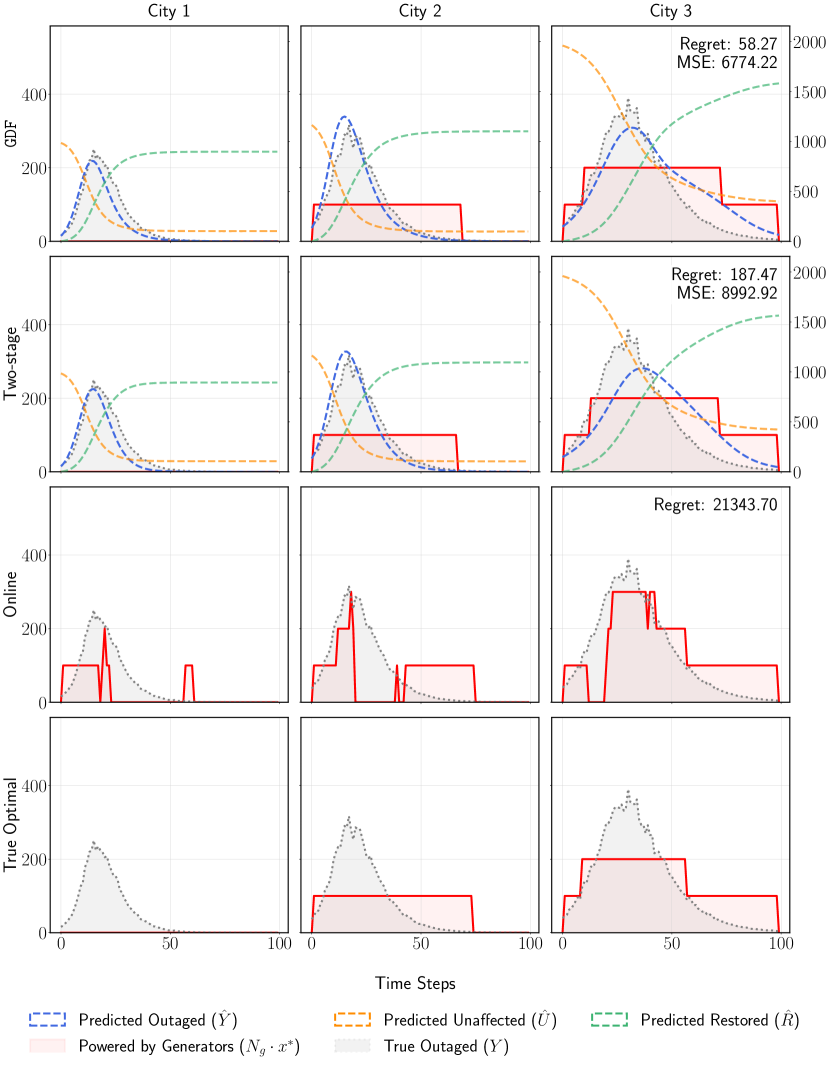
Figure 7: A synthetic example of the mobile generator deployment problem for a system with three cities and five generators ($Q_{w}=3$). The $y$-axis represents the number of outaged households. In this example, the transportation cost is set to $c=1000$, the customer interruption cost is $\tau=1$, and the operational cost is $\gamma=2$.

Figure 8: A synthetic example of the mobile generator deployment problem for a system with three cities and five generators ($Q_{w}=10$). The $y$-axis represents the number of outaged households. In this example, the transportation cost is set to $c=1000$, the customer interruption cost is $\tau=1$, and the operational cost is $\gamma=2$.

-F Additional Results for Power Line Undergrounding

Fig. 9 shows the predicted outage trajectories for all Massachusetts counties using the GDF model compared with groundtruth and Two-stage. Notably, the model exaggerates outages for selected counties—a deliberate strategy to prioritize resource allocation. This controlled overestimation, while slightly increasing MSE. Overall, it effectively reduces SAIDI and regret compared to the Two-stage baseline, demonstrating that decision-focused training can enhance overall scheduling performance.

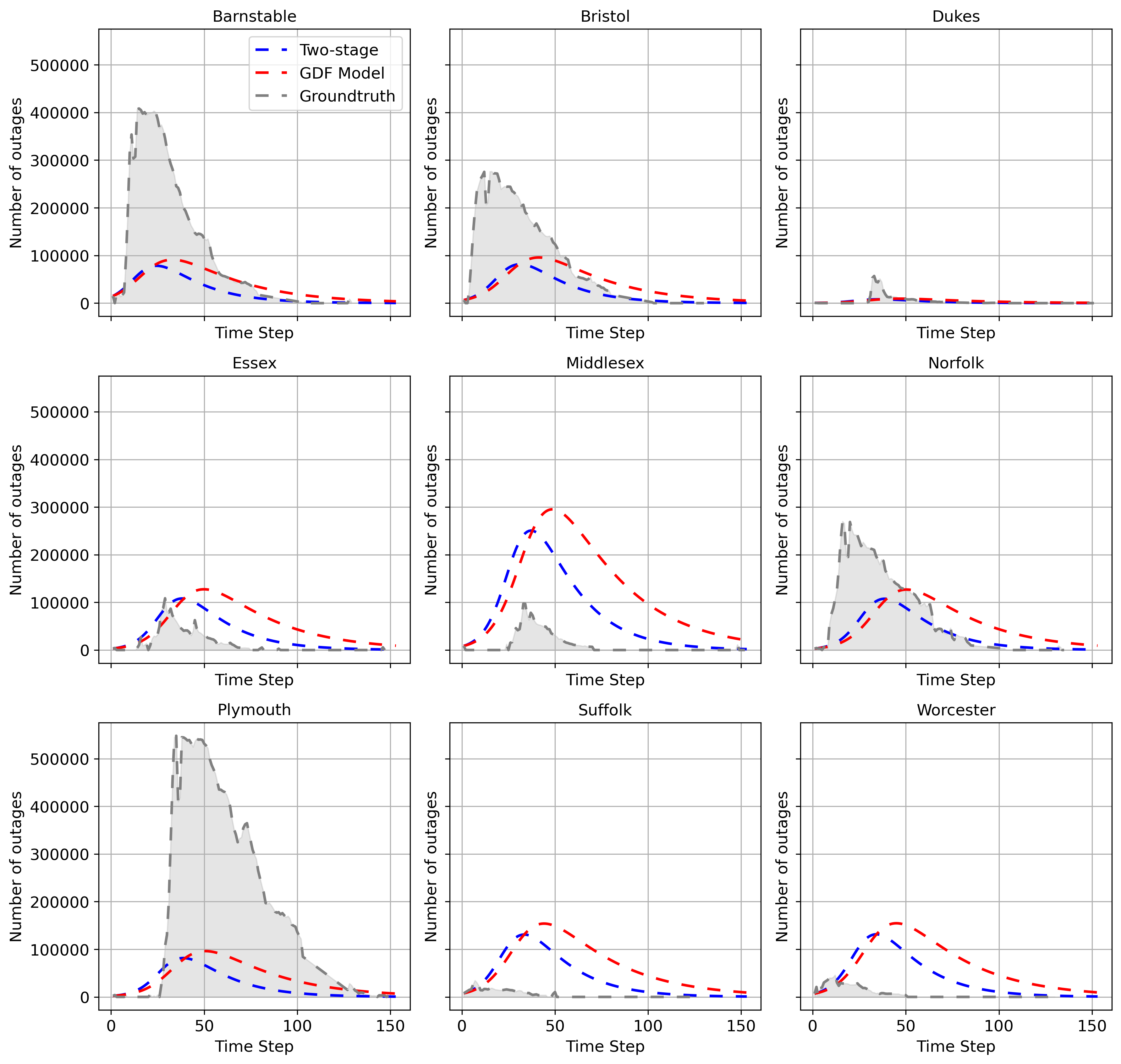
Figure 9: GDF is overestimating outage in certain counties to prioritize resource allocation at the cost of MSE.

-G Extended Literature Review for DFL and Differentiable Optimization

Decision-Focused Learning. Decision-focused learning (DFL) has emerged as a powerful framework for integrating predictive models with downstream optimization tasks. Unlike traditional two-stage approaches, which first train standalone prediction models and then use their predictions as input parameters to optimal decision models, DFL aligns the prediction model’s training loss with the objective function of the downstream optimization. This concept is enabled in gradient descent training by backpropagating gradients through the solution to an optimization problem. When the optimization is a differentiable function of its parameters, this can be implemented via implicit differentiation of optimality conditions such as KKT conditions [33, 34] or fixed-point conditions [35, 36]. When the optimization is nondifferentiable, it can instead be implemented by means of various approximation techniques [47, 9]. Unlike traditional two-stage approaches, which first train standalone prediction models and then use their predictions as inputs for decision-making, DFL directly embeds the optimization problem within the learning process. This allows the learning model to focus on the variables that matter most for the final decision [9].

Elmachtoub and Grigas [8] first proposed the Smart Predict-and-Optimize (SPO) framework, which introduced a novel method for formulating optimization problems in the prediction process. SPO essentially bridges the gap between predictive modeling and optimization by constructing a decision-driven loss function that reflects the downstream task. However, the SPO framework only addresses linear optimization problems and does not extend well to more complex combinatorial tasks.

The most-studied class of nondifferentiable optimization problems in decision-focused learning (DFL) involves linear programs (LPs). Notably, the Smart Predict-and-Optimize (SPO) framework by Elmachtoub and Grigas [8] introduced a convex surrogate upper bound to approximate subgradients for minimizing the suboptimality of LP solutions based on predicted cost coefficients. The most-studied class of nondifferentiable optimizations are linear programs (LPs). Elmachtoub and Grigas [8] proposed the Smart Predict-and-Optimize (SPO) framework for minimizing the suboptimality of solutions to a linear program as a function of its predicted cost coefficients. Despite this function being inherently non-differentiable, a convex surrogate upper-bound is used to derive informative subgradients. Wilder et al. [42] propose to smooth linear programs by augmenting their objectives with small quadratic terms [33] and differentiating the resulting KKT conditions. A method of smoothing LP’s by noise perturbations was proposed in [38]. Differentiation through combinatorial problems, such as mixed-integer programs (MIPs), is generally performed by adapting the approaches proposed for LP’s, either directly or on their LP relaxations. For example, Mandi et al. [41] demonstrated the effectiveness of the SPO method in predicting cost coefficients to MIPs. Vlastelica et al. [37] demonstrated their method directly on MIPs, and Wilder et al. [42] evaluated their approach on LP relaxations of MIPs.

Building on these works, we extend DFL to spatio-temporal decision-making for power grid resilience management. Our approach employs quadratic relaxations to enable gradient backpropagation through MIPs [42], thereby integrating a spatio-temporal ODE model for power outage forecasting directly into the optimization process. Additionally, we introduce a Global Decision-Focused Framework that combine prediciton error with decision losses across geophysical units, improving grid resilience against extreme natural events and bridging the gap between localized predictions and system-wide decisions.

Differentiable Optimization. Differentiable optimization (DO) techniques have demonstrated significant potential in integrating predictive models with optimization problems. By enabling the computation of gradients through optimization processes, DO facilitates the seamless incorporation of complex system objectives into machine learning models, thereby enhancing decision-making capabilities [44]. Recent extensions of DO methods have tackled challenges beyond standard optimization tasks. For example, distributionally robust optimization (DRO) problems have been addressed using differentiable frameworks to handle prediction tasks under worst-case scenarios. For instance, [45, 46] employed DO-based techniques to improve uncertainty quantification and robust learning, effectively addressing data scarcity and enhancing resilience modeling.

Beyond predictive modeling, DO has advanced solutions in combinatorial and nonlinear optimization. Techniques such as implicit differentiation of KKT conditions [33] and fixed-point conditions [35] address differentiable constraints, while approximation methods, including noise perturbation [38] and smoothing techniques [37], enable gradient computation for nondifferentiable tasks.

These advancements underscore DO’s pivotal role in bridging predictive modeling and optimization, especially where decision quality critically affects system resilience. In this work, DO is employed to align spatio-temporal outage predictions with grid optimization objectives, enabling robust strategies for generator deployment and power line undergrounding.

References

- [1] J. Handmer, Y. Honda, Z. W. Kundzewicz, N. Arnell, G. Benito, J. Hatfield, I. F. Mohamed, P. Peduzzi, S. Wu, B. Sherstyukov et al., “Changes in impacts of climate extremes: human systems and ecosystems,” in Managing the risks of extreme events and disasters to advance climate change adaptation special report of the intergovernmental panel on climate change. Intergovernmental Panel on Climate Change, 2012, pp. 231–290.
- [2] A. Kenward and U. Raja, “Blackout: Extreme weather climate change and power outages,” Climate central, vol. 10, pp. 1–23, 2014.
- [3] Reuters, “Over 1.3 million florida customers without power due to hurricane milton,” Reuters, October 2024, accessed: 2025-02-15. [Online]. Available: https://www.reuters.com/business/energy/over-13-million-florida-customers-without-power-due-hurricane-milton-2024-10-10/
- [4] ——, “Californian utility socal edison shuts power to over 114,000 customers due to wildfire,” Reuters, January 2025, accessed: 2025-02-15. [Online]. Available: https://www.reuters.com/business/energy/californian-utility-socal-edison-shuts-power-over-114000-customers-due-wildfire-2025-01-08/
- [5] Majlie de Puy Kamp, Curt Devine, Casey Tolan, Blake Ellis, Melanie Hicken, Rob Kuznia, Scott Glover, Yahya Abou-Ghazala, Audrey Ash, and Nelli Black, “No ‘water system in the world’ could have handled the LA fires. How the region could have minimized the damage,” CNN, 2025, [Online; accessed 14-February-2025]. [Online]. Available: https://www.cnn.com/2025/01/10/us/los-angeles-wildfires-water-system-analysis/index.html
- [6] Wikipedia contributors, “2019 California power shutoffs — Wikipedia, The Free Encyclopedia,” 2019, [Online; accessed 14-February-2025]. [Online]. Available: https://en.wikipedia.org/wiki/2019_California_power_shutoffs
- [7] Houston Chronicle Staff, “Entergy Texas invests $137 million in grid improvements to withstand extreme weather,” Houston Chronicle, 2025, [Online; accessed 14-February-2025]. [Online]. Available: https://www.houstonchronicle.com/business/energy/article/entergy-grid-improvements-extreme-weather-20034162.php
- [8] A. N. Elmachtoub and P. Grigas, “Smart “Predict, then Optimize”,” Management Science, vol. 68, no. 1, pp. 9–26, Jan. 2022, publisher: INFORMS. [Online]. Available: https://pubsonline.informs.org/doi/10.1287/mnsc.2020.3922
- [9] J. Mandi, J. Kotary, S. Berden, M. Mulamba, V. Bucarey, T. Guns, and F. Fioretto, “Decision-Focused Learning: Foundations, State of the Art, Benchmark and Future Opportunities,” Journal of Artificial Intelligence Research, vol. 80, pp. 1623–1701, Aug. 2024. [Online]. Available: https://www.jair.org/index.php/jair/article/view/15320
- [10] C. Fernández-Loría and F. Provost, “Causal decision making and causal effect estimation are not the same… and why it matters,” INFORMS Journal on Data Science, vol. 1, no. 1, pp. 4–16, 2022.
- [11] M. Massaoudi, M. Ez Eddin, A. Ghrayeb, H. Abu-Rub, and S. S. Refaat, “Advancing coherent power grid partitioning: A review embracing machine and deep learning,” IEEE Open Access Journal of Power and Energy, vol. 12, pp. 59–75, 2025.
- [12] W. Guo, Z. Xu, Z. Zhou, J. Liu, J. Wu, H. Zhao, and X. Guan, “Integrating end-to-end prediction-with-optimization for distributed hydrogen energy system scheduling*,” in 2024 IEEE 20th International Conference on Automation Science and Engineering (CASE), 2024, pp. 2774–2779.
- [13] “Massachusetts power outages,” Massachusetts Emergency Management Agency, Massachusetts, USA, Tech. Rep., 2020.
- [14] National Oceanic and Atmospheric Administration, “High-resolution rapid refresh (HRRR) model,” https://rapidrefresh.noaa.gov/hrrr/, 2024, accessed: 2024-11-11.
- [15] U.S. Census Bureau, “American community survey 1-year estimates, data profiles: Massachusetts,” 2017, accessed: 2025-02-23. [Online]. Available: https://www.census.gov/acs/www/data/data-tables-and-tools/data-profiles/2017/
- [16] R. Deshmukh and A. Kalage, “Optimal placement and sizing of distributed generator in distribution system using artificial bee colony algorithm,” in 2018 IEEE Global Conference on Wireless Computing and Networking (GCWCN), 2018, pp. 178–181.
- [17] H. Qin, A. Moriakin, G. Xu, and J. Li, “The generator distribution problem for base stations during emergency power outage: A branch-and-price-and-cut approach,” European Journal of Operational Research, vol. 318, no. 3, pp. 752–767, 2024. [Online]. Available: https://www.sciencedirect.com/science/article/pii/S0377221724004351
- [18] N. A. Ahmed and M. F. AlHajri, “Distributed generators optimal placement and sizing in power systems,” in 2019 IEEE 6th International Conference on Engineering Technologies and Applied Sciences (ICETAS), 2019, pp. 1–5.
- [19] J. Qiu, L. J. Reedman, Z. Y. Dong, K. Meng, H. Tian, and J. Zhao, “Network reinforcement for grid resiliency under extreme events,” in 2017 IEEE Power & Energy Society General Meeting, 2017, pp. 1–5.
- [20] S. Bu, F. R. Yu, P. X. Liu, and P. Zhang, “Distributed scheduling in smart grid communications with dynamic power demands and intermittent renewable energy resources,” in 2011 IEEE International Conference on Communications Workshops (ICC), 2011, pp. 1–5.
- [21] H. Aydin, R. Melhem, D. Mosse, and P. Mejia-Alvarez, “Dynamic and aggressive scheduling techniques for power-aware real-time systems,” in Proceedings 22nd IEEE Real-Time Systems Symposium (RTSS 2001) (Cat. No.01PR1420), 2001, pp. 95–105.
- [22] J. Giri, “Proactive management of the future grid,” IEEE Power and Energy Technology Systems Journal, vol. 2, no. 2, pp. 43–52, 2015.
- [23] P. Fairley, “Utilities bury transmission lines,” IEEE Spectrum, vol. 55, no. 2, pp. 9–10, 2018.
- [24] M. Panteli, D. N. Trakas, P. Mancarella, and N. D. Hatziargyriou, “Power systems resilience assessment: Hardening and smart operational enhancement strategies,” Proceedings of the IEEE, vol. 105, no. 7, pp. 1202–1213, 2017.
- [25] N. Abi-Samra, L. Willis, and M. Moon, Hardening the System, 2013. [Online]. Available: https://www.tdworld.com/vegetation-management/article/20962556/hardening-the-system
-
[26]
D. Shea, Hardening the Grid: How States Are Working to Establish a Resilient and Reliable Electric System, 2018, available online:
urlhttps://www.ncsl.org/research/energy/hardening-the-grid-how-states-are-working-to-establish-a-resilient-and-reliable-electric-system.aspx [Accessed: February 14, 2025]. - [27] M. Macaš, S. Orlando, S. Costea, P. Novák, O. Chumak, P. Kadera, and P. Kopejtko, “Impact of forecasting errors on microgrid optimal power management,” in 2020 IEEE International Conference on Environment and Electrical Engineering and 2020 IEEE Industrial and Commercial Power Systems Europe (EEEIC / I&CPS Europe), 2020, pp. 1–6.
- [28] R. Eskandarpour and A. Khodaei, “Machine learning based power grid outage prediction in response to extreme events,” IEEE Transactions on Power Systems, vol. 32, no. 4, pp. 3315–3316, 2017.
- [29] F. Yang, D. W. Wanik, D. Cerrai, M. A. E. Bhuiyan, and E. N. Anagnostou, “Quantifying uncertainty in machine learning-based power outage prediction model training: A tool for sustainable storm restoration,” Sustainability, vol. 12, no. 4, 2020. [Online]. Available: https://www.mdpi.com/2071-1050/12/4/1525
- [30] A. Zhang, W. Zhou, L. Xie, and S. Zhu, “Recurrent neural goodness-of-fit test for time series,” arXiv preprint arXiv:2410.13986, 2024.
- [31] R. T. Q. Chen, Y. Rubanova, J. Bettencourt, and D. Duvenaud, “Neural ordinary differential equations,” in Proceedings of the 32nd International Conference on Neural Information Processing Systems, ser. NIPS’18. Red Hook, NY, USA: Curran Associates Inc., 2018, p. 6572–6583.
- [32] C. Qian and A. Wang, “Power grid disturbance prediction and analysis method based on SIR model,” in 2021 IEEE 4th Student Conference on Electric Machines and Systems (SCEMS), 2021, pp. 1–5.
- [33] B. Amos and J. Z. Kolter, “OptNet: Differentiable optimization as a layer in neural networks,” in Proceedings of the 34th International Conference on Machine Learning, ser. Proceedings of Machine Learning Research, vol. 70. PMLR, 2017, pp. 136–145.
- [34] S. Gould, R. Hartley, and D. Campbell, “Deep declarative networks,” IEEE Transactions on Pattern Analysis and Machine Intelligence, vol. 44, no. 8, pp. 3988–4004, 2021.
- [35] J. Kotary, M. H. Dinh, and F. Fioretto, “Backpropagation of unrolled solvers with folded optimization,” arXiv preprint arXiv:2301.12047, 2023.
- [36] B. Wilder, E. Ewing, B. Dilkina, and M. Tambe, “End to end learning and optimization on graphs,” Advances in Neural Information Processing Systems, vol. 32, 2019.
- [37] M. Vlastelica, A. Paulus, V. Musil, G. Martius, and M. Rolínek, “Differentiation of blackbox combinatorial solvers,” arXiv preprint arXiv:1912.02175, 2019.
- [38] Q. Berthet, M. Blondel, O. Teboul, M. Cuturi, J.-P. Vert, and F. Bach, “Learning with differentiable pertubed optimizers,” Advances in neural information processing systems, vol. 33, pp. 9508–9519, 2020.
- [39] V. D. Vito, M. Mohammadian, K. Baker, and F. Fioretto, “Learning to solve differential equation constrained optimization problems,” in International Conference on Learning Representations, vol. 13, 2025.
- [40] A. Jacquillat, M. L. Li, M. Ramé, and K. Wang, “Branch-and-price for prescriptive contagion analytics,” Operations Research, vol. Ahead of Print, 2024. [Online]. Available: https://doi.org/10.1287/opre.2023.0308
- [41] J. Mandi, P. J. Stuckey, T. Guns et al., “Smart predict-and-optimize for hard combinatorial optimization problems,” in Proceedings of the AAAI Conference on Artificial Intelligence, vol. 34, no. 02, 2020, pp. 1603–1610.
- [42] B. Wilder, B. Dilkina, and M. Tambe, “Melding the data-decisions pipeline: Decision-focused learning for combinatorial optimization,” in Proceedings of the AAAI Conference on Artificial Intelligence, vol. 33, no. 01, 2019, pp. 1658–1665.
- [43] P. Z. Wang, J. Liang, S. Chen, F. Fioretto, and S. Zhu, “Gen-dfl: Decision-focused generative learning for robust decision making,” 2025. [Online]. Available: https://arxiv.org/abs/2502.05468
- [44] A. Agrawal, B. Amos, S. Barratt, S. Boyd, S. Diamond, and Z. Kolter, “Differentiable convex optimization layers,” in Advances in Neural Information Processing Systems, 2019.
- [45] S. Zhu, L. Xie, M. Zhang, R. Gao, and Y. Xie, “Distributionally robust weighted k-nearest neighbors,” Advances in Neural Information Processing Systems, vol. 35, pp. 29 088–29 100, 2022.
- [46] S. Chen, K. Ding, and S. Zhu, “Uncertainty-aware robust learning on noisy graphs,” in Proceedings of the IEEE International Conference on Acoustics, Speech, and Signal Processing (ICASSP), 2025. [Online]. Available: https://arxiv.org/abs/2306.08210
- [47] J. Kotary, F. Fioretto, P. Van Hentenryck, and B. Wilder, “End-to-end constrained optimization learning: A survey,” in Proceedings of the Thirtieth International Joint Conference on Artificial Intelligence, IJCAI-21, 2021, pp. 4475–4482. [Online]. Available: https://doi.org/10.24963/ijcai.2021/610
- [48] S. Zhu, R. Yao, Y. Xie, F. Qiu, Y. Qiu, and X. Wu, “Quantifying grid resilience against extreme weather using large-scale customer power outage data,” 2021.
- [49] V. S. Rajkumar, A. Ştefanov, J. L. Rueda Torres, and P. Palensky, “Dynamical analysis of power system cascading failures caused by cyber attacks,” IEEE Transactions on Industrial Informatics, vol. 20, no. 6, pp. 8807–8817, 2024.
- [50] C. Kosma, G. Nikolentzos, G. Panagopoulos, J.-M. Steyaert, and M. Vazirgiannis, “Neural ordinary differential equations for modeling epidemic spreading,” Transactions on Machine Learning Research, 2023.
- [51] A. Ratha, E. Iggland, and G. Andersson, “Value of lost load: How much is supply security worth?” in 2013 IEEE Power & Energy Society General Meeting, 2013, pp. 1–5.
- [52] Wikipedia contributors, “March 11–15, 2018 nor’easter,” 2023, [Online; accessed 23-February-2025]. [Online]. Available: https://en.wikipedia.org/wiki/March_11%E2%80%9315,_2018_nor%27easter
- [53] L. Xie, X. Zheng, Y. Sun, T. Huang, and T. Bruton, “Massively digitized power grid: Opportunities and challenges of use-inspired ai,” Proceedings of the IEEE, vol. 111, no. 7, pp. 762–787, 2023.
- [54] J. W. Muhs, M. Parvania, and M. Shahidehpour, “Wildfire risk mitigation: A paradigm shift in power systems planning and operation,” IEEE Open Access Journal of Power and Energy, vol. 7, pp. 366–375, 2020.
- [55] S. Kramer, T. Rodenbaugh, and M. Conroy, “The use of trenchless technologies for transmission and distribution projects,” in Proceedings of IEEE/PES Transmission and Distribution Conference, 1994, pp. 302–308.
- [56] “IEEE guide for electric power distribution reliability indices,” IEEE Std 1366-2022 (Revision of IEEE Std 1366-2012), pp. 1–44, 2022.