A microlocal pathway to spectral asymmetry:
curl and the eta invariant

Abstract

The notion of eta invariant is traditionally defined by means of analytic continuation. We prove, by examining the particular case of the operator curl, that the eta invariant can equivalently be obtained as the trace of the difference of positive and negative spectral projections, appropriately regularised. Our construction is direct, in the sense that it does not involve analytic continuation, and is based on the use of pseudodifferential techniques. This provides a novel approach to the study of spectral asymmetry of non-semibounded (pseudo)differential systems on manifolds which encompasses and extends previous results.

Keywords: curl, spectral asymmetry, eta invariant, pseudodifferential projections.

2020 MSC classes: primary 58J50; secondary 35P20, 35Q61, 47B93, 47F99; 58J28, 58J40.

1 Statement of the problem

The study of spectral asymmetry, namely, the difference in the distribution of positive and negative eigenvalues of (pseudo)differential operators on manifolds is a well-established area of pure mathematics, initiated by Atiyah, Patodi and Singer in their seminal series of papers [1, 2, 3, 4]. The classical approach to the subject goes as follows. Given a non-semibounded self-adjoint first order (pseudo)differential operator with (real) eigenvalues $\{\lambda_{k}\}$, one introduces the quantity

$$\eta(s):=\sum_{\lambda_{k}\neq 0}\frac{\operatorname{sgn}(\lambda_{k})}{|\lambda_{k}|^{s}},\qquad s\in\mathbb{C},$$

called the eta function of the operator. After showing that the eta function can be defined as a meromorphic function in the whole complex plane with no pole at $s=0$, one declares the value $\eta(0)$, called eta invariant of the operator, to be a measure of the spectral asymmetry of the operator. The motivation underpinning this definition is that for a self-adjoint operator acting in a finite-dimensional vector space the quantity $\eta(0)$ is precisely the number of positive eigenvalues minus the number of negative eigenvalues. Let us mention that one can also define a local version of the eta function, where each term in the infinite series is weighted by the modulus squared of the corresponding eigenfuncions, and for which similar results can be proved — see, e.g., [14, 6].

The eta invariant, a geometric invariant, turned out to be an incredibly powerful concept with far-reaching consequences across analysis, geometry, and beyond. For instance, it features in the Atiyah–Singer Index Theorem for elliptic operators on manifolds with boundary, to name but one of its most well-known applications. The existing body of work on the topic is massive, especially in the case of Dirac and Dirac-type operators, hence we do not even attempt a systematic review of the literature, which would go beyond the scope of the current paper. We shall just emphasise that most of the existing approaches hinge on a combination of techniques from complex analysis (analytic continuation) and differential topology (characteristic classes), often relying on black-box-type arguments.

This paper completes the analysis initiated in [12], resulting in a new, direct approach to the study of eta functions (both local and global) and eta invariants through the prism of microlocal analysis, starting from a less well-studied, yet fundamental, operator: the operator curl. We refer the reader to [12] for a more detailed review of existing literature.

Let $(M,g)$ be a connected closed oriented Riemannian manifold of dimension $d=3$. We denote by $\rho(x):=\sqrt{\det g_{\alpha\beta}(x)}$ the Riemannian density and by $\Omega^{k}=\Omega^{k}(M)$, $0\leq k\leq 3$, the space of real-valued $k$-forms over $M$. Furthermore, we denote by $*$, $\mathrm{d}$ and $\delta$ the Hodge dual, the exterior derivative (differential) and the codifferential, respectively. Finally, we denote by $\operatorname{Riem}$, $\operatorname{Ric}$ and $\operatorname{Sc}$ the Riemann tensor, the Ricci tensor and scalar curvature. We refer the reader to [12, Appendix A] for our differential geometric conventions.

We equip $\Omega^{k}(M)$ with the $L^{2}$ inner product

$$\langle u,v\rangle:=\int_{M}*u\wedge v=\int_{M}u\wedge*v\,,$$ (1.1)

where $\wedge$ is the exterior product of differential forms, and define $H^{s}(M)$, $s>0$, to be the space of differential forms that are square integrable together with their partial derivatives up to order $s$. We do not carry in our notation for Sobolev spaces the degree of differential forms: this will be clear from the context. Henceforth, to further simplify notation we drop the $M$ and write $\Omega^{k}$ for $\Omega^{k}(M)$ and $H^{s}$ for $H^{s}(M)$.

Hodge’s Theorem [15, Corollary 3.4.2] tells us that $\Omega^{k}$ decomposes into a direct sum of three orthogonal closed subspaces

$$\Omega^{k}=\mathrm{d}\Omega^{k-1}\oplus\delta\Omega^{k+1}\oplus\mathcal{H}^{k},$$

where $\mathrm{d}\Omega^{k-1}$, $\delta\Omega^{k+1}$ and $\mathcal{H}^{k}$ are the Hilbert subspaces of exact, coexact and harmonic $k$-forms, respectively.

Definition 1.1.

We define $\operatorname{curl}$ to be the operator

$$\operatorname{curl}=*\mathrm{d}:\delta\Omega^{2}\cap H^{1}\to\delta\Omega^{2}\,.$$ (1.2)

Observe that Definition 1.1 makes sense, because $*\mathrm{d}$ maps coexact 1-forms to coexact 1-forms. It is well-known — see, e.g., [18, 5] and [12, Theorem 2.1] — that $\operatorname{curl}$ as defined by (1.2) is a self-adjoint operator with discrete spectrum accumulating to both $+\infty$ and $-\infty$. Furthermore, zero is not an eigenvalue of $\operatorname{curl}$. Note, however, that $\operatorname{curl}$ is not elliptic. Indeed, the formula for the principal symbol of $\operatorname{curl}$ (which happens to coincide with its full symbol) reads

$$[\operatorname{curl}_{\mathrm{prin}}]_{\alpha}{}^{\beta}(x,\xi)=-i\,E_{\alpha}{}^{\beta\gamma}(x)\,\xi_{\gamma}\,,$$ (1.3)

where the tensor $E$ is defined in accordance with

$$E_{\alpha\beta\gamma}(x):=\rho(x)\,\varepsilon_{\alpha\beta\gamma}$$ (1.4)

and $\varepsilon$ is the totally antisymmetric symbol, $\varepsilon_{123}:=+1$. A straightforward calculation shows that

$$\det(\operatorname{curl}_{\mathrm{prin}})=0.$$

The eigenvalues of $\operatorname{curl}_{\mathrm{prin}}$ are simple and read

$$h^{(0)}(x,\xi)=0,\qquad h^{(\pm)}(x,\xi)=\pm\|\xi\|\,,$$

for all $(x,\xi)\in T^{*}M\setminus\{0\}$, where

$$\|\xi\|:=\sqrt{g^{\mu\nu}(x)\,\xi_{\mu}\xi_{\nu}}\,.$$

Consequently, standard elliptic theory does not apply and particular care is required when studying the spectrum of $\operatorname{curl}$.

Let $\lambda_{j}$ be the eigenvalues of $\operatorname{curl}$ and $u_{j}$ its orthonormalised eigenforms. Here we enumerate using positive integers $j$ for positive eigenvalues and negative integers $j$ for negative eigenvalues, so that

$$-\infty\leftarrow\ldots\leq\lambda_{-2}\leq\lambda_{-1}<0<\lambda_{1}\leq\lambda_{2}\leq\ldots\rightarrow+\infty\,,$$

with account of multiplicities.

Definition 1.2.

We define the local eta function for the operator $\operatorname{curl}$ as

$$\eta_{\operatorname{curl}}^{\mathrm{loc}}(x;s):=\sum_{j\in\mathbb{Z}\setminus\{0\}}\frac{\operatorname{sgn}\lambda_{j}}{|\lambda_{j}|^{s}}\,*(u_{j}\wedge*u_{j})(x)\,,$$ (1.5)

where $*(u_{j}\wedge*u_{j})(x)=g^{\alpha\beta}(x)\,[u_{j}]_{\alpha}(x)\,[u_{j}]_{\beta}(x)$ is the pointwise norm squared of the eigenform $u_{j}$.

We define the (global) eta function for the operator $\operatorname{curl}$ as

$$\eta_{\operatorname{curl}}(s):=\sum_{k\in\mathbb{Z}\setminus\{0\}}\frac{\operatorname{sgn}\lambda_{k}}{|\lambda_{k}|^{s}}\,.$$ (1.6)

It is not hard to show that the series (1.6) converges absolutely for $\operatorname{Re}s>3$ and defines a meromorphic function in $\mathbb{C}$ by analytic continuation, with possible first order poles at $s=3,2,1,0,-1,-2,\dots$. Furthermore, it is holomorphic at $s=0$, see [1, 2, 3, 4]. Similarly, for any fixed $x\in M$, the series (1.5) converges absolutely for $\operatorname{Re}s>3$ and defines a meromorphic function in $\mathbb{C}$ by analytic continuation, with possible first order poles at $s=3,2,1,-1,-2,\dots$. It is shown in [7] that, in fact, $s\mapsto\eta_{\operatorname{curl}}(s)$ and, for each $x\in M$, $s\mapsto\eta_{\operatorname{curl}}^{\mathrm{loc}}(x;s)$ are holomorphic in the half-plane $\operatorname{Re}s>-1$; in fact, this also follows from the arguments presented in Section 7.

Of course, the local and global eta functions are related via the identity

$$\eta_{\operatorname{curl}}(s)=\int_{M}\eta_{\operatorname{curl}}^{\mathrm{loc}}(x;s)\,\rho(x)\,\mathrm{d}x\,.$$

Definition 1.3.

We call the real-valued function $\eta_{\operatorname{curl}}^{\mathrm{loc}}(x;0)$ the local eta invariant for the operator $\operatorname{curl}$, and we call the scalar $\eta_{\operatorname{curl}}(0)$ the eta invariant for the operator $\operatorname{curl}$.

The overall philosophy of our paper is to avoid the “black box” of analytic continuation and approach the eta invariant intuitively, namely,

$$\eta_{\operatorname{curl}}(0)=\#\{\text{positive eigenvalues}\}\,-\,\#\{\text{negative eigenvalues}\}\,.$$

Indeed, for a self-adjoint operator in a finite-dimensional inner product space the quantity $\eta(0)$ can be written as

$$\operatorname{Tr}(P_{+}-P_{-})$$ (1.7)

where $\operatorname{Tr}$ is the operator trace, and $P_{+}$ and $P_{-}$ are projections onto the direct sums of positive and negative eigenspaces, respectively.

Trying to give a meaning to (1.7) for the case of non-semibounded operators acting in infinite-dimensional Hilbert spaces is both the key and the starting point of our approach, whose foundations were developed in [10, 11, 9, 12] and are summarised below, for the reader’s convenience.

The issue at hand is how to rigorously define (1.7) when the projection operators $P_{+}$ and $P_{-}$ have infinite rank, and understand the meaning of the outcome.

Let us go back to the operator $\operatorname{curl}$ and let us introduce the following orthogonal projections acting in $\Omega^{1}$:

$$P_{+}:=\sum_{j=1}^{+\infty}u_{j}\langle u_{j},\,\cdot\,\rangle\,,$$ (1.8)

$$P_{-}:=\sum_{j=1}^{+\infty}u_{-j}\langle u_{-j},\,\cdot\,\rangle\,,$$ (1.9)

$$P_{0}:=-\mathrm{d}\Delta^{-1}\delta\,,$$ (1.10)

where $\Delta^{-1}$ is the pseudoinverse of the (nonpositive) Laplace–Beltrami operator $\Delta:=-\delta\mathrm{d}$. The operators $P_{+}$ and $P_{-}$ are the positive and negative spectral projections, whereas $P_{0}$ is the orthogonal projection onto exact 1-forms.

The operators (1.8)–(1.10) are related as

$$P_{+}+P_{-}+P_{0}=\operatorname{Id}-P_{\mathcal{H}^{1}},$$

where $\operatorname{Id}$ is the identity operator and $P_{\mathcal{H}}$ is the orthogonal projection onto the (finite-dimensional) subspace of harmonic 1-forms. It was shown in [12] that (1.8)–(1.10) are pseudodifferential operators of order zero, whose full symbol can be explicitly constructed via the algorithm given in [10, Section 4.3].

In what follows, we denote by $\Psi^{s}$ the space of classical pseudodifferential operators of order $s$ with polyhomogeneous symbols acting on 1-forms. Furthermore, we define

$$\Psi^{-\infty}:=\bigcap_{s}\Psi^{s}$$ (1.11)

and we write $Q=R\mod\Psi^{-\infty}$ if $Q-R$ is an integral operator with infinitely smooth integral kernel. Recall that a pseudodifferential operator $Q\in\Psi^{s}$ acting on 1-forms can be written locally as

$$Q:u_{\alpha}(x)\mapsto v_{\alpha}(x)=(2\pi)^{-d}\int e^{i(x-y)^{\gamma}\xi_{\gamma}}\,q_{\alpha}{}^{\beta}(x,\xi)\,u_{\beta}(y)\,\mathrm{d}y\,\mathrm{d}\xi\,.$$ (1.12)

The quantity

$$q_{\alpha}{}^{\beta}(x,\xi)\sim[q_{s}]_{\alpha}{}^{\beta}(x,\xi)+[q_{s-1}]_{\alpha}{}^{\beta}(x,\xi)+\dots,$$ (1.13)

is called the (full) symbol of $Q$. Here $\,\sim\,$ stands for asymptotic expansion [17, § 3.3]. The components $[q_{s-k}]_{\alpha}{}^{\beta}$ of $q_{\alpha}{}^{\beta}$ are positively homogeneous in momentum $\xi$:

$$[q_{s-k}]_{\alpha}{}^{\beta}(x,\lambda\,\xi)=\lambda^{s-k}\,[q_{s-k}]_{\alpha}{}^{\beta}(x,\xi),\qquad\forall\lambda>0,\quad k=0,1,2,\dots.$$

Observe that the indices $\alpha$ and $\beta$ in (1.13) ‘live’ at different points, $x$ and $y$ respectively. When writing (1.12) we implicitly used the same coordinate system for $x$ and $y$.

The leading homogeneous component of the symbol — a smooth matrix function on $T^{*}M\setminus\{0\}$ — is called the principal symbol of $Q$ and denoted by $Q_{\mathrm{prin}}$. We denote by $Q_{\mathrm{sub}}$ the subprincipal symbol of $Q$ — a modification of the subleading homogeneous component of the symbol of $Q$ — defined in accordance with [12, Definition 3.2]. Observe that principal and subprincipal symbols are covariant quantities under changes of local coordinates, see [12, Remark 3.3].

Throughout the paper we denote pseudodifferential operators with upper case letters, and their symbols and homogeneous components of symbols with lower case. At times we will write a pseudodifferential operator as an integral operator with distributional integral kernel (Schwartz kernel); namely, we will write (1.12) as

$$Q:u_{\alpha}(x)\mapsto\int_{M}\mathfrak{q}_{\alpha}{}^{\beta}(x,y)\,u_{\beta}(y)\,\rho(y)\,\mathrm{d}y$$ (1.14)

with

$$\mathfrak{q}_{\alpha}{}^{\beta}(x,y)=\frac{1}{(2\pi)^{d}\,\rho(y)}\int e^{i(x-y)^{\gamma}\xi_{\gamma}}\,q_{\alpha}{}^{\beta}(x,\xi)\,\mathrm{d}\xi$$

in a distributional (local) sense and modulo an infinitely smooth contribution. When we do so, we use lower case Fraktur font for the Schwartz kernel.

The key notion which allows us to tackle (1.7) is that of (pointwise) matrix trace of a pseudodifferential operator acting on 1-forms.

Definition 1.4.

Let $Q\in\Psi^{s}$. We call the matrix trace of $Q$ the scalar pseudodifferential operator $\operatorname{\mathfrak{tr}}Q$ of order $s$ defined as

$$\operatorname{\mathfrak{tr}}Q:f(x)\mapsto\int_{M}(\operatorname{\mathfrak{tr}}\mathfrak{q})(x,y)\,f(y)\,\rho(y)\,\mathrm{d}y\,,$$ (1.15)

where

$$(\operatorname{\mathfrak{tr}}\mathfrak{q})(x,y):=\mathfrak{q}_{\alpha}{}^{\beta}(x,y)\,Z_{\beta}{}^{\alpha}(y,x)\,\chi(\operatorname{dist}(x,y)/\epsilon)$$ (1.16)

is the pointwise matrix trace of the distributional kernel $\mathfrak{q}$ of $Q$.

In (1.15) $Z_{\alpha}{}^{\beta}(x,y)$ is the linear map (3.6) realising parallel transport of vectors from $x$ to $y$ along the unique shortest geodesic connecting them, $\chi:[0,+\infty)\to\mathbb{R}$ is a compactly supported smooth scalar function such that $\chi=1$ in a neighbourhood of zero, $\operatorname{dist}$ is the geodesic distance, and $\epsilon>0$ is a sufficiently small parameter ensuring that (1.16) vanishes when $x$ and $y$ are far away. We refer the reader to Section 3 for a more detailed description of these quantities, as well as a more thorough discussion of the properties of the matrix trace of a (pseudo)differential operator.

Note that in Definition 1.4 we write $\operatorname{\mathfrak{tr}}$ with Fraktur font to emphasise the fact that (1.16) is not the standard matrix trace $\mathrm{tr}$, but it involves parallel transport.

The essential idea underpinning Definition 1.4 is to decompose the operation of taking the (operator) trace of an operator acting on 1-forms which is, a priori, not necessarily of trace class, into two separate steps: first one takes the matrix trace of the original operator, thus obtaining a scalar pseudodifferential operator, then one takes the operator trace of the resulting scalar operator, in the hope that cancellations along the way would make the latter operation legitimate.

Remarkably, this turns out to be the case for the operator $P_{+}-P_{-}$ associated with $\operatorname{curl}$.

Definition 1.5.

We define the asymmetry operator to be the self-adjoint scalar pseudodifferential operator

$$A:=\operatorname{\mathfrak{tr}}(P_{+}-P_{-})\,,$$ (1.17)

where $P_{\pm}$ are the operators (1.8)–(1.9) and $\operatorname{\mathfrak{tr}}$ is the matrix trace (1.15).

Prima facie, $A$ is an operator of order zero. It was shown in [12, Theorem 1.4] that $A$ is, in fact, a pseudodifferential operator of order $-3$ (hence almost of trace class) with principal symbol

$$A_{\mathrm{prin}}(x,\xi)=-\frac{1}{2\|\xi\|^{5}}E^{\alpha\beta\gamma}(x)\,\nabla_{\alpha}\operatorname{Ric}_{\beta}{}^{\rho}(x)\,\xi_{\gamma}\xi_{\rho}\,.$$ (1.18)

A careful analysis of the leading singularity of the integral kernel $\mathfrak{a}$ of the operator $A$ — essentially encoded within (1.18) — allowed us to prove the following result in [12].

Theorem 1.6 ([12, Theorem 1.6]).

The integral kernel $\mathfrak{a}(x,y)$ of the asymmetry operator $A$ is a bounded function, smooth outside the diagonal. Furthermore, for any $x\in M$ the limit

$$\psi_{\operatorname{curl}}^{\mathrm{loc}}(x):=\lim_{r\to 0^{+}}\frac{1}{4\pi r^{2}}\int_{\mathbb{S}_{r}(x)}\mathfrak{a}(x,y)\,\mathrm{d}S_{y}$$ (1.19)

exists and defines a continuous scalar function $\,\psi_{\operatorname{curl}}^{\mathrm{loc}}:M\to\mathbb{R}\,$. Here $\mathbb{S}_{r}(x)=\{y\in M|\operatorname{dist}(x,y)=r\}$ is the sphere of radius $r$ centred at $x$ and $\mathrm{d}S_{y}$ is the surface area element on this sphere.

Definition 1.7.

We call the function $\psi_{\operatorname{curl}}^{\mathrm{loc}}:M\to\mathbb{R}$ the regularised local trace of $\operatorname{curl}$ and the number

$$\psi_{\operatorname{curl}}:=\int_{M}\psi_{\operatorname{curl}}^{\mathrm{loc}}(x)\,\rho(x)\,\mathrm{d}x$$

the regularised global trace of $\operatorname{curl}$.

These two quantities are geometric invariants, in that they are determined by the Riemannian 3-manifold and its orientation. In particular, the global regularised trace is a real number measuring the asymmetry of the spectrum of $\operatorname{curl}$.

In [12] we claimed that $\psi_{\operatorname{curl}}$ is precisely the classical eta invariant and that $\psi_{\operatorname{curl}}^{\mathrm{loc}}$ is the local eta invariant, only defined in a purely analytic fashion, via microlocal analysis. The main goal of this paper is to prove this claim.

Notation

Symbol	Description
$\sim$	Asymptotic expansion
$\ast$	Hodge dual
$\|\,\cdot\,\|$	Riemannian norm
$|\,\cdot\,|$	Euclidean norm
$A$	Asymmetry operator, Definition 1.5
$A^{(s)}$	Parameter-dependent asymmetry operator, Definition 2.2
$A^{(s)}_{\mathrm{diag}}$, $A^{(s)}_{\mathrm{pt}}$	Local decomposition of $A^{(s)}$ as per (4.20) and (4.21)
$\mathfrak{a}(x,y)$	Integral kernel of the asymmetry operator $A$
$\mathfrak{a}^{(s)}(x,y)$	Integral kernel of the asymmetry operator $A$
$\operatorname{curl}$	The operator curl (1.1)
$d$	Dimension of the manifold $M$, $d\geq 2$
$\mathrm{d}$	Exterior derivative
$\delta$	Codifferential
$\Delta:=-\delta\mathrm{d}$	(Nonpositive) Laplace–Beltrami operator
$\bm{\Delta}:=-(\mathrm{d}\delta+\delta\mathrm{d})$	(Nonpositive) Hodge Laplacian
$\operatorname{dist}$	Geodesic distance
$\varepsilon_{\alpha\beta\gamma}$	Totally antisymmetric symbol, $\varepsilon_{123}=+1$
$E_{\alpha\beta\gamma}$	Totally antisymmetric tensor (1.4)
$f_{x^{\alpha}}$	Partial derivative of $f$ with respect to $x^{\alpha}$
$g$	Riemannian metric
$\Gamma^{\alpha}{}_{\beta\gamma}$	Christoffel symbols
$\eta_{Q}^{\mathrm{loc}}(x;s)$	Local eta function of the operator $Q$ (formula (1.5) for $Q=\operatorname{curl}$)
$\eta_{Q}(s)$	Eta function of the operator $Q$ (formula (1.6) for $Q=\operatorname{curl}$)
$H^{s}(M)$	Generalisation of the usual Sobolev spaces $H^{s}$ to differential forms
$\mathcal{H}^{k}(M)$	Harmonic $k$-forms over $M$
$(\lambda_{j},u_{j})$, $j=\pm 1,\pm 2,\ldots$	Eigensystem for $\operatorname{curl}$
$\theta$	Heaviside theta function
$\operatorname{I}$	Identity matrix
$\operatorname{Id}$	Identity operator
$(\mu_{j},f_{j})$, $j=0,1,2,\ldots$	Eigensystem for $-\Delta$
$M$	Connected closed oriented Riemannian manifold
$\operatorname{mod}\ \Psi^{-\infty}$	Modulo an integral operator with infinitely smooth kernel
$P_{0}$, $P_{\pm}$	Orthogonal projections (1.10) and (1.8), (1.9)
$p_{\pm}(x,y)$	Full symbol of $P_{\pm}$
$Q_{\mathrm{prin}}$	Principal symbol of the pseudodifferential operator $Q$
$Q_{\mathrm{sub}}$	Subprincipal symbol of $Q$, for operators on 1-forms see [12, Definition 3.2]
$R_{\lambda}$	Resolvent $(-\bm{\Delta}-\lambda\mathrm{I})^{-1}$ of $-\bm{\Delta}$
$\mathrm{Ref}^{(s)}$	Reference operator, Definition 6.1
$\mathfrak{ref}^{(s)}(x,y)$	Scalar function (6.2) and distribution (6.6)
$\operatorname{Riem}$, $\operatorname{Ric}$, $\operatorname{Sc}$	Riemann curvature tensor, Ricci tensor, scalar curvature
$\rho(x)$	Riemannian density
$\mathbb{S}_{r}(x)$	Geodesic sphere of radius $r$ centred at $x\in M$
$\operatorname{\mathfrak{tr}}$	(Pointwise) matrix trace, Definition 1.4
$\operatorname{Tr}$	Operator trace
$TM$, $T^{*}M$	Tangent and cotangent bundle
$\Omega^{k}(M)$	Differential $k$-forms over $M$
$\psi_{\operatorname{curl}}^{\mathrm{loc}}(x)$	Regularised local trace of $A$, Definition 1.7
$\psi_{\operatorname{curl}}$	Regularised global trace of $A$, Definition 1.7
$\Psi^{s}$	Classical pseudodifferential operators of order $s$
$\Psi^{-\infty}$	Infinitely smoothing operators (1.11)
$Z$	Parallel transport map (3.6)

2 Main results

The centrepiece of our paper is the following result.

Theorem 2.1.

The regularised local trace of the asymmetry operator coincides with the local eta invariant and the regularised global trace of the asymmetry operator coincides with the eta invariant. Namely,

$$\psi_{\operatorname{curl}}^{\mathrm{loc}}(x)=\eta_{\operatorname{curl}}^{\mathrm{loc}}(x;0)\,,$$

$$\psi_{\operatorname{curl}}=\eta_{\operatorname{curl}}(0)\,.$$

This completes the analysis initiated in [12] and provides a new approach to the study of spectral asymmetry of non-semibounded (pseudo)differential systems on manifolds which possesses the following main elements of novelty.

• We characterise asymmetry of the spectrum in terms of a pseudodifferential operator of negative order, as opposed to a single number. The classical geometric invariants can be recovered by computing the local and global regularised operator traces of the asymmetry operator. In this sense, our approach encompasses and extends previous results.

• The overarching idea is not specific to $\operatorname{curl}$, but can be deployed for a variety of operators. For example, we will be applying it to the massless Dirac operator in a separate paper.

• Our construction is direct, in the sense that it does not involve analytic continuation, and is based on the use of pseudodifferential techniques and explicit computations.

• It implements in a rigorous fashion the intuitive understanding of spectral asymmetry as the difference between the number of positive and negative eigenvalues.

The strategy for proving Theorem 2.1 is as follows.

Let us introduce a one-parameter family of pseudodifferential operators defined as follows.

Definition 2.2.

Let $s$ be a real number. We define the parameter-dependent asymmetry operator as

$$A^{(s)}:=\operatorname{\mathfrak{tr}}\left[(P_{+}-P_{-})(-\bm{\Delta})^{-s/2}\right]\,,$$ (2.1)

where $\bm{\Delta}$ is the (nonpositive) Hodge Laplacian acting on 1-forms.

Prima facie, for a given $s\in\mathbb{R}$ the operator (2.1) is a pseudodifferential operator of order $-s$. Furthermore, it is not hard to to see that for $s>3$ the operator $A^{(s)}$ is of trace class, and that its operator trace is the eta function $\eta_{\operatorname{curl}}(s)$ — full justification for these claims will be provided in Section 4.

A deeper analysis reveals that, very much like the asymmetry operator (1.17), $A^{(s)}$ enjoys higher smoothing properties than initially expected.

Theorem 2.3.

a

1. The operator $A^{(s)}$ is a self-adjoint pseudodifferential operator of order $-s-3$.

2. The principal symbol of the operator $A^{(s)}$ reads

   $$(A^{(s)})_{\mathrm{prin}}(x,\xi)=-\frac{(s+1)(s+3)}{6\,\|\xi\|^{s+5}}\,E^{\alpha\beta\gamma}(x)\,\nabla_{\alpha}\operatorname{Ric}_{\beta}{}^{\rho}(x)\,\xi_{\gamma}\xi_{\rho}\,.$$ (2.2)

Remark 2.4.

Formula (2.2) tells us that the principal symbol of the operator $A^{(s)}$ vanishes at $s=-1$ and $s=-3$. In fact, a stronger result is true: the operator $A^{(s)}$ itself vanishes at $s=-1$ and $s=-3$. Indeed, according to formulae (4.1) and (4.3) we have $\,A^{(-k)}=\operatorname{\mathfrak{tr}}(\operatorname{curl}^{k})\,$ for odd natural $k$, whereas Propositions 3.4 and 3.5 tell us that $\,\operatorname{\mathfrak{tr}}\operatorname{curl}=\operatorname{\mathfrak{tr}}(\operatorname{curl}^{3})=0\,$.

Theorem 2.3 part (a) allows us to extend our earlier claim about the operator $A^{(s)}$ being trace class from $s>3$ all the way up to $s>0$.

Theorem 2.5.

Let $\mathfrak{a}^{(s)}(x,y)$ be the integral kernel of $A^{(s)}$. For $s>0$ we have

$$\mathfrak{a}^{(s)}(x,x)=\eta_{\operatorname{curl}}^{\mathrm{loc}}(x;s)$$

and

$$\operatorname{Tr}A^{(s)}=\eta_{\operatorname{curl}}(s)\,.$$

Remark 2.6.

Note that $s\in(0,+\infty)$ is the maximal interval in which $A^{(s)}$ is of trace class. Indeed, $A^{(0)}=A$ is not of trace class in general, as demonstrated in [12, Sections 6 and 7].

Next, one observes that for $s=0$ the operator $A^{(s)}$ turns into the asymmetry operator $A$ — cf. (1.17) and (2.1). Furthermore, comparing (1.18) with (2.2) we see that

$$(A^{(s)})_{\mathrm{prin}}=f(s)\,A_{\mathrm{prin}}\qquad\text{with}\qquad f(s)=\frac{(s+1)(s+3)}{3\,\|\xi\|^{s}}\,.$$

Proving Theorem 2.5, which in turn will imply Theorem 2.1, requires one to carefully examine the behaviour of the integral kernel of $A^{(s)}$ as $s\to 0^{+}$. Let us emphasise that there are several nontrivial (and somewhat subtle) obstacles one needs to overcome in order to achieve this. In particular, one has to find a way to “follow the singularity” of $\mathfrak{a}^{(s)}$ up to $s=0^{+}$ in such a way that the error terms brought about by the microlocal approach do not grow in an uncontrolled fashion when the parameter $s$ becomes smaller and smaller.

Structure of the paper

Our paper is structured as follows.

In Section 3 we revisit the notion of matrix trace of an operator, building on the analysis from [12, Section 4]. In particular, we provide stronger results for differential (as opposed to pseudodifferential) matrix operators.

In Section 4 we perform a detailed examination of the parameter-dependent asymmetry operator $A^{(s)}$: we discuss its basic properties, prove that it is a pseudodifferential operator of order $-s-3$, and compute its principal symbol.

Section 5 establishes a precise relationship between the operator $A^{(s)}$ and the local and global eta functions of the operator curl. This prepares the ground for Section 6, which features a careful analysis of the leading singularity of the integral kernel of $A^{(s)}$. The latter is achieved by defining a reference operator which captures the leading singularity and underpins our notion of (regularised) trace for $A^{(s)}$.

Finally, in Section 7 we give the proof of our main result, Theorem 2.1

Our paper is complemented by a section with concluding remarks, Section 8, and three appendices with auxiliary technical material.

3 The matrix trace of an operator, revisited

In this section we will briefly summarise and revisit the notion of matrix trace of a pseudodifferential operator acting on 1-forms introduced in [12, Section 4]. We refer the reader to [12, Section 4] for further details and a broader discussion.

Consider a pseudodifferential operator

$$Q:u_{\alpha}(x)\mapsto\int_{M}\mathfrak{q}_{\alpha}{}^{\beta}(x,y)\,u_{\beta}(y)\,\rho(y)\,\mathrm{d}y$$

of order $s$ acting on 1-forms, with scalar integral kernel $\mathfrak{q}_{\alpha}{}^{\beta}$ (Schwartz kernel).

There are two natural notions of trace associated with $Q$. The first notion is that of operator trace $\operatorname{Tr}Q$, which is well defined when the operator is of trace class. This is the case if $s<-d$ and the operator is self-adjoint. The second notion is that of matrix trace $\operatorname{\mathfrak{tr}}Q$, introduced in Definition 1.4. The latter produces a scalar pseudodifferential operator of the same order as the original operator $Q$.

It was shown in [12, Section 4] that the matrix trace satisfies the following properties.

1. The operator $\operatorname{\mathfrak{tr}}Q$ is defined uniquely, modulo the addition of a scalar integral operator whose integral kernel is infinitely smooth and vanishes in a neighbourhood of the diagonal.

2. $(\operatorname{\mathfrak{tr}}Q)^{*}=\operatorname{\mathfrak{tr}}(Q^{*})$, where the star refers to formal adjoints with respect to the natural inner products. In particular, if $Q$ is self-adjoint, then so is $\operatorname{\mathfrak{tr}}Q$.

3. If $s<-d$ and the operator $Q$ is self-adjoint then

   $$\operatorname{Tr}(\operatorname{\mathfrak{tr}}Q)=\operatorname{Tr}Q\,.$$ (3.1)

4. We have

   $$(\operatorname{\mathfrak{tr}}Q)_{\mathrm{prin}}=\operatorname{tr}Q_{\mathrm{prin}},$$ (3.2)

   $$(\operatorname{\mathfrak{tr}}Q)_{\mathrm{sub}}=\operatorname{tr}Q_{\mathrm{sub}}\,.$$ (3.3)

5. The quantities on the left-hand sides of (3.1)–(3.3) are independent of the parameter $\epsilon$ appearing in formula (1.16).

When $Q:u_{\alpha}\mapsto Q_{\alpha}{}^{\beta}\,u_{\beta}$ is a differential operator acting on 1-forms, one has a stronger result. In order to formulate this result, let us write down the operator $Q$ in local coordinates:

$$Q_{\alpha}{}^{\beta}=\sum_{|\bm{\kappa}|\leq m}[q^{\bm{\kappa}}]_{\alpha}{}^{\beta}(x)\,\frac{\partial^{|\bm{\kappa}|}}{\partial x^{\bm{\kappa}}}\,,$$ (3.4)

where $m$ is the order of the differential operator, $\bm{\kappa}=(\kappa_{1},\dots,\kappa_{d})\in\mathbb{N}_{0}^{d}$ is a multi-index, $|\bm{\kappa}|=\sum_{j=1}^{d}\kappa_{j}$ and $\displaystyle\frac{\partial^{|\bm{\kappa}|}}{\partial x^{\bm{\kappa}}}=\frac{\partial^{|\bm{\kappa}|}}{\partial(x^{1})^{\kappa_{1}}\dots\partial(x^{d})^{\kappa_{d}}}\,$. Then introduce another differential operator

$$R_{\alpha}{}^{\beta}(x):=\sum_{|\bm{\kappa}|\leq m}[q^{\bm{\kappa}}]_{\alpha}{}^{\beta}(x)\,\frac{\partial^{|\bm{\kappa}|}}{\partial y^{\bm{\kappa}}}$$ (3.5)

which acts in the variable $y$, whereas the variable $x$ plays the role of parameter.

Recall that

$$Z:T_{x}M\ni u^{\alpha}\mapsto u^{\alpha}\,Z_{\alpha}{}^{\beta}(x,y)\in T_{y}M$$ (3.6)

is the linear map realising parallel transport of vectors from $x$ to $y$ along the unique shortest geodesic connecting $x$ and $y$. In what follows, we raise and lower indices in the 2-point tensor $Z_{\alpha}{}^{\beta}(x,y)$ using the Riemannian metric $g(x)$ in the first index and $g(y)$ in the second.

Recall also the identity [12, formula (4.9)]

$$Z_{\beta}{}^{\alpha}(y,x)=Z^{\alpha}{}_{\beta}(x,y).$$ (3.7)

Proposition 3.1.

Let $Q$ be a differential operator acting on 1-forms and $R(x)$ be the corresponding parameter-dependent differential operator defined, in local coordinates, in accordance with formula (3.5). Then $\operatorname{\mathfrak{tr}}Q$ is the scalar differential operator

$$\operatorname{\mathfrak{tr}}Q:f(x)\mapsto\left.[R_{\alpha}{}^{\beta}(x)\,Z_{\beta}{}^{\alpha}(y,x)\,f(y)]\right|_{y=x}\,.$$ (3.8)

Proof.

Let $U\subseteq M$ be a coordinate patch and let $x$ be local coordinates in $U$. We assume that $U$ is small enough so that for all $x,y\in U$ we have $\chi(\operatorname{dist}(x,y)/\epsilon)=1$, where $\epsilon$ is the parameter appearing in formula (1.16).

In what follows, without loss of generality, the infinitely smooth 1-form $u$ and scalar function $f$ are assumed to be compactly supported in $U$. This is acceptable because differential operators are local, unlike the more general pseudodifferential operators.

In our coordinate patch and chosen local coordinates the differential operators $Q_{\alpha}{}^{\beta}$ read (3.4). The operator $Q$ can now be equivalently rewritten in integral form as

$$Q:u_{\alpha}(x)\mapsto\frac{1}{(2\pi)^{d}}\int e^{i(x-y)^{\gamma}\xi_{\gamma}}\,q_{\alpha}{}^{\beta}(x,\xi)\,u_{\beta}(y)\,\mathrm{d}y\,\mathrm{d}\xi\,,$$ (3.9)

where

$$q_{\alpha}{}^{\beta}(x,\xi)=\sum_{|\bm{\kappa}|\leq m}i^{|\bm{\kappa}|}\,[q^{\bm{\kappa}}]_{\alpha}{}^{\beta}(x)\,\xi_{\bm{\kappa}}$$

is the (left) symbol of $Q$. Here $\xi_{\bm{\kappa}}=(\xi_{1})^{\kappa_{1}}\dots(\xi_{d})^{\kappa_{d}}$.

Formulae (1.14)–(1.16) and (3.9) imply

$$\operatorname{\mathfrak{tr}}Q:f(x)\mapsto\frac{1}{(2\pi)^{d}}\int e^{i(x-y)^{\gamma}\xi_{\gamma}}\,q_{\alpha}{}^{\beta}(x,\xi)\,Z_{\beta}{}^{\alpha}(y,x)\,f(y)\,\,\mathrm{d}y\,\mathrm{d}\xi\,.$$ (3.10)

Examination of formula (3.10) shows that we are looking at (3.8). ∎

We feel it necessary to provide an alternative equivalent reformulation of Proposition 3.1, one that avoids the use of the parameter-dependent differential operator (3.5). Let is instead make use of the amplitude-to-symbol operator

$$\mathcal{S}_{\mathrm{left}}\sim\sum_{k=0}^{+\infty}\mathcal{S}_{\mathrm{-k}},\qquad\mathcal{S}_{0}:=\left.(\,\cdot\,)\right|_{y=x},\qquad\mathcal{S}_{-k}:=\frac{1}{k!}\left.\left[\left(-i\dfrac{\partial^{2}}{\partial y^{\gamma}\partial\xi_{\gamma}}\right)^{k}(\,\cdot\,)\right]\right|_{y=x},$$ (3.11)

see [12, formula (3.13)]. The action of the operator (3.11) on an amplitude $q(x,y,\xi)$ of a (pseudo)differential operator excludes the $y$-dependence, i.e. gives the (left) symbol. Note that the operator (3.11) maps an amplitude polynomial in $\xi$ to a (left) symbol polynomial in $\xi$.

Proposition 3.2.

Let $Q$ be a differential operator acting on 1-forms with (left) symbol $q_{\alpha}{}^{\beta}(x,\xi)$. Then $\operatorname{\mathfrak{tr}}Q$ is the scalar differential operator with (left) symbol

$$\mathcal{S}_{\mathrm{left}}\,[q_{\alpha}{}^{\beta}(x,\xi)\,Z_{\beta}{}^{\alpha}(y,x)]\,.$$ (3.12)

Proof.

Consequence of formula (3.10) and the definition of the amplitude-to-symbol operator. ∎

Remark 3.3.

It is easy to see that if $Q$ is a pseudodifferential operator acting on 1-forms with (left) symbol $q_{\alpha}{}^{\beta}(x,\xi)$, then $\operatorname{\mathfrak{tr}}Q$ is the scalar pseudodifferential operator with (left) symbol given by formula (3.12). Of course, in the pseudodifferential case symbols are not polynomials in $\xi$ and are defined modulo $O(|\xi|^{-\infty})$ as $|\xi|\to+\infty$.

To conclude this section, we will examine some important examples of matrix trace. In preparation for this analysis, recall that in geodesic normal coordinates centred at $x=0$ the metric admits the expansion

$$g_{\alpha\beta}(y)=\delta_{\alpha\beta}-\frac{1}{3}\operatorname{Riem}_{\alpha\mu\beta\nu}(0)\,y^{\mu}y^{\nu}+O(|y|^{3})\,,$$ (3.13)

so that one has $\,\displaystyle\det g_{\alpha\beta}(y)=1-\frac{1}{3}\operatorname{Ric}_{\mu\nu}(0)\,y^{\mu}y^{\nu}+O(|y|^{3})\,$ and

$$\rho(y)=1-\frac{1}{6}\operatorname{Ric}_{\mu\nu}(0)\,y^{\mu}y^{\nu}+O(|y|^{3})\,.$$ (3.14)

Furthermore, the parallel transport map $Z^{\alpha}{}_{\beta}(x,y)$ admits the following expansion [12, formula (E.2)]

$$Z^{\alpha}{}_{\beta}(0,y)=\delta^{\alpha}{}_{\beta}-\frac{1}{6}\operatorname{Riem}^{\alpha}{}_{\mu\beta\nu}(0)\,y^{\mu}y^{\nu}+\frac{1}{6}\frac{\partial^{2}\Gamma^{\alpha}{}_{\mu\beta}}{\partial y^{\nu}\partial y^{\rho}}(0)\,y^{\mu}y^{\nu}y^{\rho}+O(|y|^{4})\,.$$ (3.15)

Proposition 3.4.

In dimension $d=3$ we have

$$\operatorname{\mathfrak{tr}}\operatorname{curl}=0\,.$$ (3.16)

Proof.

Formula (3.8) applied to $Q=\operatorname{curl}$ gives us

$$\operatorname{\mathfrak{tr}}\operatorname{curl}:f(x)\mapsto\left.\left[-E_{\alpha}{}^{\beta\gamma}(x)\,\frac{\partial}{\partial y^{\gamma}}\,Z_{\beta}{}^{\alpha}(y,x)\,f(y)\right]\right|_{y=x}\,.$$ (3.17)

Let us choose geodesic normal coordinates centred at $x=0$. Then formulae (3.17), (1.4), (3.13), (3.14), (3.7) and (3.15) immediately imply (3.16). ∎

Proposition 3.5.

In dimension $d=3$ we have

$$\operatorname{\mathfrak{tr}}(\operatorname{curl}^{3})=0\,.$$

Proof.

We are looking at the differential operator $Q=\operatorname{curl}^{3}\,$,

$$Q_{\alpha}{}^{\beta}=-E_{\alpha}{}^{\gamma\rho}(x)\,\frac{\partial}{\partial x^{\rho}}\left(E_{\gamma}{}^{\mu\sigma}(x)\,\frac{\partial}{\partial x^{\sigma}}\left(E_{\mu}{}^{\beta\tau}(x)\,\frac{\partial}{\partial x^{\tau}}\right)\right).$$ (3.18)

We need to rewrite (3.18) in the form (3.4), i.e. put all the coefficients in front of partial derivatives, and then form the parameter-dependent differential operator $R(x)$ in accordance with formula (3.5).

Let us choose geodesic normal coordinates centred at $x=0$. A somewhat lengthy but straightforward calculation shows that in the chosen coordinate system the differential operator $R(0)$ reads

$$R_{\alpha}{}^{\beta}(0)=\left[\varepsilon^{\beta\rho\tau}\operatorname{Ric}_{\alpha\rho}(0)-\frac{1}{3}\varepsilon_{\alpha}{}^{\beta\rho}\operatorname{Ric}_{\rho}{}^{\tau}(0)\,+\frac{1}{3}\varepsilon_{\alpha}{}^{\tau\rho}\operatorname{Ric}_{\rho}{}^{\beta}(0)\right]\frac{\partial}{\partial y^{\tau}}\\ +\varepsilon_{\alpha}{}^{\beta\rho}\,\frac{\partial}{\partial y^{\rho}}\left(\delta^{\sigma\tau}\frac{\partial^{2}}{\partial y^{\sigma}\partial y^{\tau}}\right).$$ (3.19)

In writing down (3.19) we used (1.4), (3.13), (3.14) and the elementary identity

$$\varepsilon_{\alpha\beta\gamma}\,\varepsilon^{\mu\nu\gamma}=\delta_{\alpha}{}^{\mu}\delta_{\beta}{}^{\nu}-\delta_{\alpha}{}^{\nu}\delta_{\beta}{}^{\mu}.$$

It only remains to substitute (3.19), (3.7) and (3.15) into the RHS of (3.8) at $x=0$.

We consider separately the contributions to (3.8) from the three terms on the RHS of (3.15).

The contribution from the first term on the RHS of (3.15) vanishes because $\,R_{\alpha}{}^{\beta}(0)\,\delta^{\alpha}{}_{\beta}=0\,$.

The contribution from the second term on the RHS of (3.15) reads

$$-\,\frac{1}{3}\,\varepsilon_{\alpha}{}^{\beta\rho}\,\operatorname{Ric}^{\alpha}{}_{\beta}(0)\,\left.\frac{\partial f}{\partial y^{\rho}}\right|_{y=0}-\,\frac{1}{3}\,\varepsilon_{\alpha}{}^{\beta\rho}\,[\operatorname{Riem}^{\alpha}{}_{\rho\beta}{}^{\sigma}(0)+\operatorname{Riem}^{\alpha\sigma}{}_{\beta\rho}(0)]\left.\frac{\partial f}{\partial y^{\sigma}}\right|_{y=0}\,.$$

The tensors $\,\operatorname{Ric}^{\alpha\beta}(0)\,$ and $\,\operatorname{Riem}^{\alpha\rho\beta\sigma}(0)+\operatorname{Riem}^{\alpha\sigma\beta\rho}(0)\,$ are symmetric in $\alpha,\beta$, hence the expression (3) vanishes.

Note that the fact that the second term on the RHS of (3.15) gives a zero contribution to the RHS of (3.8) at $x=0$ can be established without involving the explicit formula (3). In dimension three the Riemann curvature tensor is expressed via the Ricci tensor, so we are looking at a linear combination of terms of the form

$$\varepsilon_{\alpha\beta\gamma}\times\operatorname{Ric}_{\kappa\lambda}\times\left.\frac{\partial f}{\partial y^{\mu}}\right|_{y=0}\,.$$

Here one has to perform contraction of indices to get a scalar. It is easy to see that any such contraction gives zero.

The proof of Proposition 3.5 has been reduced to examining the contribution to (3.8) coming from the third term on the RHS of (3.15). Namely, the task at hand is to show that

$$\varepsilon_{\alpha}{}^{\beta\rho}\,\frac{\partial}{\partial y^{\rho}}\left(\delta^{\sigma\tau}\frac{\partial^{2}}{\partial y^{\sigma}\partial y^{\tau}}\right)\frac{\partial^{2}\Gamma^{\alpha}{}_{\mu\beta}}{\partial y^{\nu}\partial y^{\gamma}}(0)\,y^{\mu}y^{\nu}y^{\gamma}=0\,.$$

But $\partial^{2}\Gamma$ is expressed via $\nabla\operatorname{Ric}\,$, so we are looking at a linear combination of terms of the form

$$\varepsilon_{\alpha\beta\gamma}\times\nabla_{\kappa}\operatorname{Ric}_{\lambda\mu}\,.$$

Here one has to perform contraction of indices to get a scalar. It is easy to see that any such contraction gives zero. This completes the proof of Proposition 3.5. ∎

Proposition 3.6.

In any dimension $d\geq 2$ we have

$$\operatorname{\mathfrak{tr}}\bm{\Delta}=d\Delta-\operatorname{Sc}\,,$$ (3.20)

where $\bm{\Delta}$ is the (nonpositive) Hodge Laplacian acting on 1-forms, $\Delta$ is the (nonpositive) Laplace–Beltrami operator and $\operatorname{Sc}$ is scalar curvature.

Proof.

The (nonpositive) Hodge Laplacian $\bm{\Delta}$ acting on 1-forms is defined by formula

$$\bm{\Delta}=-(\mathrm{d}\delta+\delta\mathrm{d})\,.$$ (3.21)

In local coordinates we have

$$(\mathrm{d}\delta)_{\alpha}{}^{\beta}=-\frac{\partial}{\partial x^{\alpha}}\,\rho^{-1}\,\frac{\partial}{\partial x^{\gamma}}\,g^{\gamma\beta}\,\rho\,,$$ (3.22)

$$(\delta\mathrm{d})_{\alpha}{}^{\beta}=g_{\alpha\nu}\,\rho^{-1}\,\frac{\partial}{\partial x^{\mu}}\left(g^{\mu\beta}\,g^{\nu\gamma}-g^{\mu\gamma}\,g^{\nu\beta}\right)\rho\,\frac{\partial}{\partial x^{\gamma}}\,.$$ (3.23)

In (3.22) and (3.23) it is understood that partial derivatives act on everything to their right.

We are looking at the differential operator $Q=\bm{\Delta}$ defined by formulae (3.21)–(3.23). We need to rewrite it in the form (3.4), i.e. put all the coefficients in front of partial derivatives, and then form the parameter-dependent differential operator $R(x)$ in accordance with formula (3.5).

As in the proof of Proposition 3.5, let us choose geodesic normal coordinates centred at $x=0$. A straightforward calculation based on the use of formulae (3.13) and (3.14) shows that in the chosen coordinate system the differential operator $R(0)$ reads

$$R_{\alpha}{}^{\beta}(0)=\delta_{\alpha}{}^{\beta}\left(\delta^{\mu\gamma}\frac{\partial^{2}}{\partial y^{\mu}\partial y^{\gamma}}\right)-\frac{2}{3}\operatorname{Ric}_{\alpha}{}^{\beta}(0)\,.$$ (3.24)

We now substitute (3.24), (3.7) and (3.15) into the RHS of (3.8) at $x=0$.

We consider separately the contributions to (3.8) from the first two terms on the RHS of (3.15).

The contribution from the first term on the RHS of (3.15) reads $\displaystyle\,d\left(\delta^{\mu\gamma}\frac{\partial^{2}}{\partial y^{\mu}\partial y^{\gamma}}\right)-\frac{2}{3}\operatorname{Sc}(0)\,$, whereas the contribution from the second term on the RHS of (3.15) reads $\displaystyle\,-\frac{1}{3}\operatorname{Sc}(0)\,$. Hence, in geodesic normal coordinates centred at $x=0$ we have

$$[\,(\operatorname{\mathfrak{tr}}\bm{\Delta})f\,](0)=\left.\left[\,d\left(\delta^{\mu\gamma}\frac{\partial^{2}f}{\partial y^{\mu}\partial y^{\gamma}}\right)-\operatorname{Sc}f\,\right]\right|_{y=0}\,.$$ (3.25)

Comparing (3.25) with the action of the Laplace–Beltrami operator $\displaystyle\,\Delta=\rho^{-1}\,\frac{\partial}{\partial y^{\mu}}\,g^{\mu\nu}\,\rho\,\frac{\partial}{\partial y^{\nu}}\,$, we arrive at (3.20). ∎

4 The parameter-dependent asymmetry operator $A^{(s)}$

In this section we will examine the parameter-dependent asymmetry operator $A^{(s)}$ introduced in Definition 2.2 and establish its basic properties. In particular, we will prove Theorem 2.3.

4.1 An alternative representation for $A^{(s)}$

To start with, let us provide an alternative representation for the operator $A^{(s)}$.

Let

$$0=\mu_{0}<\mu_{1}\leq\mu_{2}\leq\dots\to+\infty$$

be the eigenvalues of the operator $-\Delta$ enumerated in increasing order and with account of multiplicity, and let $f_{j}$, $j=0,1,2,\dots$, be the corresponding orthonormalised eigenfunctions. Here $\Delta$ is the (nonpositive) Laplace–Beltrami operator.

Recall also that $(\lambda_{j},u_{j})$, $j\in\mathbb{Z}\setminus\{0\}$, is our notation the eigensystem of $\operatorname{curl}$.

Lemma 4.1.

a

1. We have

   $$A^{(s)}=\operatorname{\mathfrak{tr}}\left[\operatorname{curl}\,(-\bm{\Delta})^{-\frac{s+1}{2}}\right].$$ (4.1)

2. If $s>3$ the operator $A^{(s)}$ is of trace class.

Proof.

(a) The family of 1-forms $v_{j}:=\mu_{j}^{-1/2}\mathrm{d}f_{j}$, $j=1,2,\dots$, forms an orthonormal basis for the Hilbert space $\mathrm{d}\Omega^{0}$ with inner product (1.1). Since on a Riemannian 3-manifold the codifferential $\delta$ acts on $\Omega^{k}$ as $\,\delta=(-1)^{k}*\mathrm{d}\,*\,$, the Spectral Theorem gives us the following representation for the (nonpositive) Hodge Laplacian (3.21) acting on 1-forms:

$$\bm{\Delta}=-(\mathrm{d}\delta+\delta\mathrm{d})=-\sum_{j=1}^{+\infty}\mu_{j}\,v_{j}\langle v_{j},\,\cdot\,\rangle-\sum_{j\in\mathbb{Z}\setminus\{0\}}\lambda_{j}^{2}\,u_{j}\langle u_{j},\,\cdot\,\rangle\,.$$ (4.2)

Hence,

$$(-\bm{\Delta})^{r}=(\mathrm{d}\delta+\delta\mathrm{d})^{r}=\sum_{j=1}^{+\infty}\mu_{j}^{r}\,v_{j}\langle v_{j},\,\cdot\,\rangle+\sum_{j\in\mathbb{Z}\setminus\{0\}}|\lambda_{j}|^{2r}\,u_{j}\langle u_{j},\,\cdot\,\rangle\,,\qquad r\in\mathbb{R}\,.$$ (4.3)

Formulae (1.8), (1.9) and (4.3) and Hodge’s decomposition imply

$$P_{+}-P_{-}=\operatorname{curl}\,(-\bm{\Delta})^{-1/2}\,.$$ (4.4)

Substituting (4.4) into (2.1) we obtain (4.1).

(b) Examination of formula (2.1) or formula (4.1) shows that for $s>3$ the order of the pseudodifferential operator $A^{(s)}$ is strictly less than $\,-3\,$. But a self-adjoint pseudodifferential operator of order strictly less than $\,-3\,$ is of trace class (recall that the dimension of $M$ is 3). ∎

Although at first glance the meaning of (4.1) is less transparent than that of (2.1), the representation (4.1) will be especially convenient in the forthcoming calculations because it involves the composition of a power of the Hodge Laplacian with the differential operator $\operatorname{curl}$, as opposed to the pseudodifferential operator $P_{+}-P_{-}$. Indeed, from a microlocal perspective $\operatorname{curl}$ possesses the following nice properties upon which we will rely extensively:

1. the full symbol of $\operatorname{curl}$ coincides with its principal symbol (1.3) and

2. the symbol of $\operatorname{curl}$ is linear in momentum $\xi\,$, so that

   $$\frac{\partial^{|\bm{\kappa}|}\,[\operatorname{curl}_{\mathrm{prin}}]_{\alpha}{}^{\beta}}{\partial\xi_{\bm{\kappa}}}(x,\xi)=0$$ (4.5)

   for all multi-indices $\bm{\kappa}\in\mathbb{N}_{0}^{3}$ with $|\bm{\kappa}|\geq 2$.

4.2 The order of $A^{(s)}$

The goal of this subsection is to prove part (a) of Theorem 2.3. Namely, we will show that the operator $A^{(s)}$ is of order $-s-3$. This will be achieved in several steps, decreasing the order of $A^{(s)}$ at each step.

The first step is the simplest, in that it does not require extensive use of the resolvent.

Lemma 4.2.

The parameter-dependent asymmetry operator $A^{(s)}$ is a pseudodifferential operator of order $-s-2$.

Proof.

The claim is equivalent to the following two statements:

$$(A^{(s)})_{\mathrm{prin}}=0\,,$$ (4.6)

$$(A^{(s)})_{\mathrm{sub}}=0\,.$$ (4.7)

Here the subprincipal symbol of a pseudodifferential operator acting on 1-forms is defined in accordance with [12, Definition 3.2].

Formula (4.6) follows from (4.1), (3.2), (1.3) and the fact that

$$[(-\bm{\Delta})^{-\frac{s+1}{2}}]_{\mathrm{prin}}=\|\xi\|^{-\frac{s+1}{2}}\,\mathrm{I}$$ (4.8)

is proportional to the identity matrix $\operatorname{I}\,$.

Theorem 3.8 from [12] tells us that

$$[\operatorname{curl}\,(-\bm{\Delta})^{-\frac{s+1}{2}}]_{\mathrm{sub}}=\operatorname{curl}_{\mathrm{prin}}[(-\bm{\Delta})^{-\frac{s+1}{2}}]_{\mathrm{sub}}+\operatorname{curl}_{\mathrm{sub}}[(-\bm{\Delta})^{-\frac{s+1}{2}}]_{\mathrm{prin}}\\ +\frac{i}{2}\{\{\operatorname{curl}_{\mathrm{prin}},[(-\bm{\Delta})^{-\frac{s+1}{2}}]_{\mathrm{prin}}\}\}\,,$$ (4.9)

where

$$\{\{Q_{\mathrm{prin}},R_{\mathrm{prin}}\}\}_{\alpha}{}^{\beta}:=\left(\frac{\partial[Q_{\mathrm{prin}}]_{\alpha}{}^{\kappa}}{\partial x^{\gamma}}-\Gamma^{\alpha^{\prime}}{}_{\gamma\alpha}[Q_{\mathrm{prin}}]_{\alpha^{\prime}}{}^{\kappa}+\Gamma^{\kappa}{}_{\gamma\kappa^{\prime}}[Q_{\mathrm{prin}}]_{\alpha}{}^{\kappa^{\prime}}\right)\frac{\partial[R_{\mathrm{prin}}]_{\kappa}{}^{\beta}}{\partial\xi_{\gamma}}\\ -\frac{\partial[Q_{\mathrm{prin}}]_{\alpha}{}^{\kappa}}{\partial\xi_{\gamma}}\left(\frac{\partial[R_{\mathrm{prin}}]_{\kappa}{}^{\beta}}{\partial x^{\gamma}}-\Gamma^{\kappa^{\prime}}{}_{\gamma\kappa}[R_{\mathrm{prin}}]_{\kappa^{\prime}}{}^{\beta}+\Gamma^{\beta}{}_{\gamma\beta^{\prime}}[R_{\mathrm{prin}}]_{\kappa}{}^{\beta^{\prime}}\right)$$ (4.10)

is the generalised Poisson bracket. Furthermore, [12, Lemma 3.6] tells us that

$$\operatorname{curl}_{\mathrm{sub}}=0$$ (4.11)

and Lemma A.3 tells us that

$$[(-\bm{\Delta})^{-\frac{s+1}{2}}]_{\mathrm{sub}}=0.$$ (4.12)

Finally, a straightforward calculation involving (1.3), (4.8) and (4.10) gives us

$$\{\{\operatorname{curl}_{\mathrm{prin}},[(-\bm{\Delta})^{-\frac{s+1}{2}}]_{\mathrm{prin}}\}\}=0.$$ (4.13)

Substituting (4.11)–(4.13) into (4.9) we obtain

$$[\operatorname{curl}\,(-\bm{\Delta})^{-\frac{s+1}{2}}]_{\mathrm{sub}}=0\,.$$ (4.14)

Formula (4.7) then follows from (4.1), (3.3) and (4.14). ∎

In view of Lemma 4.2, formula (4.1), and formula (3.2), in order to establish that $A^{(s)}$ is of order $-s-3$ it suffices to compute the homogeneous component of the symbol of the operator $\operatorname{curl}\,(-\bm{\Delta})^{-\frac{s+1}{2}}$ of degree $-s-2$ and show that its pointwise matrix trace vanishes.

Let

$$q_{\alpha}{}^{\beta}(x,\xi)\sim\|\xi\|^{-s-1}\,\delta_{\alpha}{}^{\beta}+[q_{-s-2}]_{\alpha}{}^{\beta}(x,\xi)+[q_{-s-3}]_{\alpha}{}^{\beta}(x,\xi)+\dots$$ (4.15)

be the full symbol of the operator $(-\bm{\Delta})^{-\frac{s+1}{2}}$. Then the full symbol $t_{\alpha}{}^{\beta}$ of the operator $\operatorname{curl}\,(-\bm{\Delta})^{-\frac{s+1}{2}}$ is given by

$$t_{\alpha}{}^{\beta}(x,\xi)=E_{\alpha}{}^{\mu\gamma}(x)\left(i\xi_{\mu}\,q_{\gamma}{}^{\beta}(x,\xi)+\frac{\partial q_{\gamma}{}^{\beta}}{\partial x^{\mu}}(x,\xi)\right)\,.$$ (4.16)

In writing (4.16) we used (1.3), (4.5), and the fact that, given two pseudodifferential operators $A$ and $B$ with symbols $a$ and $b$, the symbol $\sigma_{AB}$ of their composition $AB$ is given by the formula

$$\sigma_{AB}\sim\sum_{k=0}^{\infty}\frac{1}{i^{k}k!}\dfrac{\partial^{k}a}{\partial\xi_{\alpha_{1}}\dots\partial\xi_{\alpha_{k}}}\dfrac{\partial^{k}b}{\partial x^{\alpha_{1}}\dots\partial x^{\alpha_{k}}}\,,$$ (4.17)

see [17, Theorem 3.4]. The identity (4.16) effectively reduces the task at hand to the analysis of the symbol of $(-\bm{\Delta})^{-\frac{s+1}{2}}$, the power of an elliptic differential operator.

Let us fix an arbitrary point $z\in M$ and work in geodesic normal coordinates centred at $z$. In our chosen coordinate system the operator $A^{(s)}$ (modulo $\Psi^{-\infty}$) reads

$$A^{(s)}:f(x)\mapsto\frac{1}{(2\pi)^{3}}\int e^{i(x-y)^{\mu}\xi_{\mu}}\,t_{\alpha}{}^{\beta}(x,\xi)\,Z_{\beta}{}^{\alpha}(y,x)\,f(y)\,\mathrm{d}y\,\mathrm{d}\xi\,,$$ (4.18)

where $\,t_{\alpha}{}^{\beta}(x,\xi)\,$ is defined in accordance with (4.16) and (4.15).

Next, we observe that (4.18) can be recast as

$$A^{(s)}=A^{(s)}_{\mathrm{diag}}+A^{(s)}_{\mathrm{pt}}\,,$$ (4.19)

where

$$A^{(s)}_{\mathrm{diag}}:=\frac{1}{(2\pi)^{3}}\int e^{i(x-y)^{\mu}\xi_{\mu}}\,t_{\alpha}{}^{\alpha}(x,\xi)\,f(y)\,\mathrm{d}y\,\mathrm{d}\xi$$ (4.20)

and

$$A^{(s)}_{\mathrm{pt}}:=A^{(s)}-A^{(s)}_{\mathrm{diag}}.$$ (4.21)

Here the subscript “pt” stands for “parallel transport”. Let us emphasise that the decomposition (4.19) is not invariant, i.e., it relies on our particular choice of local coordinates. However, it turns out to be very convenient when carrying out the explicit calculations below.

The following lemma establishes that the contribution from $A^{(s)}_{\mathrm{pt}}$ to the principal symbol of the parameter-dependent asymmetry operator $A^{(s)}$ at the point $z$ can be disregarded.

Lemma 4.3.

Let $a^{(s)}_{\mathrm{pt}}(x,\xi)\sim\sum_{j=0}^{+\infty}(t_{\mathrm{pt}})_{-s-j}(x,\xi)$ be the full symbol of the operator $A^{(s)}_{\mathrm{pt}}\,$. We have

$$(a^{(s)}_{\mathrm{pt}})_{-s-j}(z,\xi)=0\quad\text{for}\quad j=0,1,2,3\,.$$ (4.22)

Proof.

The claim (4.22) for $j=0$ and $j=1$ follows at once from (3.15) and (3.7). The claim (4.22) for $j=2$ and $j=3$ can be proved following the strategy from [12, subsection 6.2]. Detailed arguments are given in Appendix B. ∎

Let us further prepare the ground for the final step in the proof of Theorem 2.3, part (a).

In what follows we assume, for simplicity, that

$$s>-1\,.$$ (4.23)

The general case $s\in\mathbb{R}$ can be handled by means of [17, Proposition 10.1].

Let $R_{\lambda}:=\left(-\bm{\Delta}-\,\lambda\,\mathrm{Id}\right)^{-1}$ be the resolvent of $-\bm{\Delta}$. For fixed $(x,\xi)\in T^{*}M\setminus\{0\}$ and $\rho=\rho(x,\xi)<\|\xi\|^{2}$, let $\Gamma=\Gamma(x,\xi)=\Gamma_{1}\cup\Gamma_{2}\cup\Gamma_{3}$ be the contour in the complex plane defined by

$$\Gamma_{1}:=\{\lambda\in\mathbb{C}\ |\ \lambda=re^{i\pi},\,\rho<r<+\infty\},$$

$$\Gamma_{2}:=\{\lambda\in\mathbb{C}\ |\ \lambda=\rho\,e^{i\theta},\,-\pi<\theta<\pi\},$$

$$\Gamma_{3}:=\{\lambda\in\mathbb{C}\ |\ \lambda=re^{-i\pi},\,\rho<r<+\infty\},$$

with orientation prescribed as in the Figure 1.

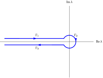
Figure 1: Contour of integration.

The classical theory of complex powers of elliptic pseudodifferential operators (see, e.g., [16], [17, § 10]) tells us that under the assumption (4.23)

$$(-\bm{\Delta})^{-\frac{s+1}{2}}=\frac{i}{2\pi}\ointclockwise_{\Gamma}\lambda^{-\frac{s+1}{2}}R_{\lambda}\,\mathrm{d}\lambda\,,$$ (4.24)

so that, arguing as in [17, § 11.2, formula (11.10)], we have

$$[q_{-s-j-1}]_{\alpha}{}^{\beta}(x,\xi)=\frac{i}{2\pi}\ointclockwise_{\Gamma}\lambda^{-\frac{s+1}{2}}[r_{-2-j}]_{\alpha}{}^{\beta}(x,\xi,\lambda)\,\mathrm{d}\lambda\,,\qquad j=0,1,2,\dots,$$ (4.25)

where

$$r_{\alpha}{}^{\beta}(x,\xi,\lambda)\sim\sum_{j=0}^{+\infty}[r_{-2-j}]_{\alpha}{}^{\beta}(x,\xi,\lambda),\qquad[r_{-2-j}]_{\alpha}{}^{\beta}(x,t\xi,t^{2}\lambda)=t^{-2-j}[r_{-2-j}]_{\alpha}{}^{\beta}(x,\xi,\lambda)\quad\forall t>0\,,$$ (4.26)

is the full symbol of $R_{\lambda}$ as a pseudodifferential operator depending on the parameter $\lambda$. Here the branch of $\lambda^{-\frac{s+1}{2}}$ is determined by making a cut along the negative real semi-axis and requiring that $\lambda^{-\frac{s+1}{2}}=1$ when $\lambda=1$.

Formula (4.25) reduces the the analysis of the symbol of $(-\bm{\Delta})^{-\frac{s+1}{2}}$ to the analysis of the symbol of $R_{\lambda}\,$.

It is easy to see that

$$[(R_{\lambda})_{\mathrm{prin}}]_{\alpha}{}^{\beta}(x,\xi,\lambda)=[r_{-2}]_{\alpha}{}^{\beta}(x,\xi,\lambda)=\frac{1}{\|\xi\|^{2}-\lambda}\,\delta_{\alpha}{}^{\beta}\,.$$ (4.27)

Note that $(R_{\lambda})_{\mathrm{prin}}(x,\xi,\lambda)$ is holomorphic in $\{|\lambda|\leq\rho\}\subset\mathbb{C}$.

The following is an auxiliary lemma which will prove to be useful in subsequent calculations.

Lemma 4.4.

We have

$$\frac{i}{2\pi}\ointclockwise_{\Gamma}\frac{\lambda^{-\frac{s+1}{2}}}{(\|\xi\|^{2}-\lambda)^{n}}\,\mathrm{d}\lambda=C_{n}(s)\,\|\xi\|^{-s-2n+1}\,,$$

where

$$C_{n}(s):=\begin{cases}1&\text{for}\quad n=1,\\ \frac{s+1}{2}&\text{for}\quad n=2,\\ \frac{(s+1)(s+3)}{8}&\text{for}\quad n=3,\\ \frac{(s+1)(s+3)(s+5)}{48}&\text{for}\quad n=4,\\ \frac{(s+1)(s+3)(s+5)(s+7)}{384}&\text{for}\quad n=5.\\ \end{cases}$$

Proof.

The claim is a straightforward consequence of Cauchy’s residue theorem. ∎

We are now in a position to state the main result of this subsection.

Proposition 4.5.

The parameter-dependent asymmetry operator $A^{(s)}$ is a pseudodifferential operator of order $-s-3$.

The proof of Proposition 4.5 consists of a careful examination of the symbol of the operator (4.1) in geodesic normal coordinates by means of formulae (4.15), (4.16), Lemma 4.3, formulae (4.24)–(4.26), and the results from Appendix A. To keep the paper to a reasonable length, we decided to omit this rather long and technical proof, on the basis that it is very similar in spirit to the proof of part (b) of Theorem 2.3, which we will give in full in the next subsection. The latter will provide a ‘quantitative version’ of the arguments required to prove Proposition 4.5.

4.3 The principal symbol of $A^{(s)}$

The goal of this subsection is to prove part (b) of Theorem 2.3. The precise expression for the principal symbol of $A^{(s)}$ will play a crucial role in the proof of the main result of our paper. This warrants providing a detailed proof.

Proof of Theorem 2.3, part (b).

As in the previous subsection, in what follows we assume to have chosen geodesic normal coordinates centred at $z=0$. In view of Lemma 4.3, proving (2.2) reduces to showing that, in the chosen coordinate system, we have

$$[t_{-s-3}]_{\alpha}{}^{\alpha}(0,\xi)=-\frac{(s+1)(s+3)}{6\,|\xi|^{s+5}}\,\varepsilon^{\alpha\beta\gamma}\,\nabla_{\alpha}\operatorname{Ric}_{\beta}{}^{\rho}(0)\,\xi_{\gamma}\xi_{\rho}\,,$$ (4.28)

where $\,t_{\alpha}{}^{\beta}(x,\xi)\,$ is defined in accordance with (4.16) and (4.15).

It is not hard to convince oneself that $A^{(s)}$ should be proportional to the covariant derivative of the Ricci tensor and the totally antisymmetric tensor $E$, see, e.g., [12, Remark 6.8]. Therefore, without loss of generality one can assume that the metric admits the following Taylor expansion in geodesic normal coordinates:

$$g_{\alpha\beta}(x)=\delta_{\alpha\beta}-\frac{1}{6}(\nabla_{\sigma}\operatorname{Riem}_{\alpha\mu\beta\nu})(0)\,x^{\sigma}\,x^{\mu}\,x^{\nu}+O(|x|^{4}).$$ (4.29)

Namely, one can assume that all components of curvature (but not their covariant derivatives) vanish at the centre of the normal coordinate system $z=0$. Formula (4.29) immediately implies

$$\rho(x)=1-\frac{1}{12}(\nabla_{\sigma}\operatorname{Ric}_{\mu\nu})(0)\,x^{\sigma}\,x^{\mu}\,x^{\nu}+O(|x|^{4}).$$

Under this assumption, the symbol of the Hodge Laplacian admits the expansion given in Theorem A.1 with $a_{1}=0$ and $a_{0}=0$.

To start with, let us note the following expressions for the partial derivatives in momentum $\xi$ of $(R_{\lambda})_{\mathrm{prin}}$ (4.27) of order $\,\leq 3\,$:

$$[(\|\xi\|^{2}-\lambda)^{-1}]_{\xi_{\mu}}=-\frac{2g^{\mu\sigma}\xi_{\sigma}}{(\|\xi\|^{2}-\lambda)^{2}}\,,$$ (4.30a)

$$[(\|\xi\|^{2}-\lambda)^{-1}]_{\xi_{\mu}\xi_{\nu}}=-\frac{2g^{\mu\nu}}{(\|\xi\|^{2}-\lambda)^{2}}+\frac{8g^{\mu\sigma}g^{\nu\rho}\xi_{\sigma}\xi_{\rho}}{(\|\xi\|^{2}-\lambda)^{3}}\,,$$ (4.30b)

$$[(\|\xi\|^{2}-\lambda)^{-1}]_{\xi_{\mu}\xi_{\nu}\xi_{\kappa}}=8\frac{g^{\mu\nu}\xi^{\kappa}+g^{\mu\kappa}\xi^{\nu}+g^{\nu\kappa}\xi^{\mu}}{(\|\xi\|^{2}-\lambda)^{3}}-\frac{48\xi^{\mu}\xi^{\nu}\xi^{\kappa}}{(\|\xi\|^{2}-\lambda)^{4}}\,.$$ (4.30c)

In formula (4.30c) and some subsequent formulae we employ, for the sake of brevity, the notation

$$\xi^{\alpha}:=g^{\alpha\beta}\xi_{\beta}\,.$$

Using formulae (4.17) and (4.27) one obtains

$$[(R_{\lambda}(-\bm{\Delta}-\lambda))_{-1}]_{\alpha}{}^{\beta}=\frac{1}{\|\xi\|^{2}-\lambda}[h_{1}]_{\alpha}{}^{\beta}+(\|\xi\|^{2}-\lambda)[r_{-3}]_{\alpha}{}^{\beta}\\ -i[(\|\xi\|^{2}-\lambda)^{-1}]_{\xi_{\mu}}(\|\xi\|^{2}-\lambda)_{x^{\mu}}\,,$$

where $[h_{1}]_{\alpha}{}^{\beta}$ is defined in accordance with (A.1), (A.4) and (A.5) and $[r_{-3}]_{\alpha}{}^{\beta}$ comes from (4.26). Formula (4.30a) and the identity $R_{\lambda}(-\bm{\Delta}-\lambda)=\mathrm{Id}$ then imply

$$[r_{-3}]_{\alpha}{}^{\beta}=-\frac{1}{(\|\xi\|^{2}-\lambda)^{2}}[h_{1}]_{\alpha}{}^{\beta}-\frac{2i}{(\|\xi\|^{2}-\lambda)^{3}}g^{\mu\gamma}\xi_{\gamma}(\|\xi\|^{2})_{x^{\mu}}\,\delta_{\alpha}{}^{\beta}\,.$$

The latter, combined with (4.25) and Lemma 4.4, in turn gives us

$$[q_{-s-2}]_{\alpha}{}^{\beta}=-\frac{s+1}{2\|\xi\|^{s+3}}[h_{1}]_{\alpha}{}^{\beta}-\frac{i(s+1)(s+3)}{4\|\xi\|^{s+5}}g^{\mu\gamma}\xi_{\gamma}(\|\xi\|^{2})_{x^{\mu}}\,\delta_{\alpha}{}^{\beta}\,,$$ (4.31)

where $[q_{-s-2}]_{\alpha}{}^{\beta}$ comes from (4.15).

Similar arguments give us

$$[r_{-4}]_{\alpha}{}^{\beta}=-\frac{1}{(\|\xi\|^{2}-\lambda)^{2}}[h_{0}]_{\alpha}{}^{\beta}\\ -\frac{1}{(\|\xi\|^{2}-\lambda)^{3}}\left[2ig^{\mu\sigma}\xi_{\sigma}([h_{1}]_{\alpha}{}^{\beta})_{x^{\mu}}+g^{\mu\nu}(\|\xi\|^{2})_{x^{\mu}x^{\nu}}\delta_{\alpha}{}^{\beta}\right]\\ +\frac{4g^{\mu\sigma}g^{\nu\rho}\xi_{\sigma}\xi_{\rho}}{(\|\xi\|^{2}-\lambda)^{4}}(\|\xi\|^{2})_{x^{\mu}x^{\nu}}\delta_{\alpha}{}^{\beta}+O(|x|^{2}|\xi|^{-4})\,,$$ (4.32)

$$[q_{-s-3}]_{\alpha}{}^{\beta}=-\frac{s+1}{2\|\xi\|^{s+3}}[h_{0}]_{\alpha}{}^{\beta}\\ -\frac{(s+1)(s+3)}{8\|\xi\|^{s+5}}\left[2ig^{\mu\sigma}\xi_{\sigma}([h_{1}]_{\alpha}{}^{\beta})_{x^{\mu}}+g^{\mu\nu}(\|\xi\|^{2})_{x^{\mu}x^{\nu}}\delta_{\alpha}{}^{\beta}\right]\\ +\frac{(s+1)(s+3)(s+5)g^{\mu\sigma}g^{\nu\rho}\xi_{\sigma}\xi_{\rho}}{12\|\xi\|^{s+7}}(\|\xi\|^{2})_{x^{\mu}x^{\nu}}\delta_{\alpha}{}^{\beta}+O(|x|^{2}|\xi|^{-s-3})\,,$$ (4.33)

$$[r_{-5}]_{\alpha}{}^{\beta}=\frac{1}{(\|\xi\|^{2}-\lambda)^{3}}\left(-2i\xi^{\mu}([h_{0}]_{\alpha}{}^{\beta})_{x^{\mu}}-g^{\mu\nu}([h_{1}]_{\alpha}{}^{\beta})_{x^{\mu}x^{\nu}}\right)\\ +\frac{1}{(\|\xi\|^{2}-\lambda)^{4}}\left(4\xi^{\mu}\xi^{\nu}([h_{1}]_{\alpha}{}^{\beta})_{x^{\mu}x^{\nu}}-\frac{8i}{3}(g^{\mu\nu}\xi^{\sigma}+g^{\mu\sigma}\xi^{\nu}+g^{\nu\sigma}\xi^{\mu})(\|\xi\|^{2})_{x^{\mu}x^{\nu}x^{\sigma}}\,\delta_{\alpha}{}^{\beta}\right)\,\\ +\frac{16i\xi^{\mu}\xi^{\nu}\xi^{\sigma}}{(\|\xi\|^{2}-\lambda)^{5}}(\|\xi\|^{2})_{x^{\mu}x^{\nu}x^{\sigma}}\,\delta_{\alpha}{}^{\beta}+O(|x||\xi|^{-5})\,,$$ (4.34)

$$[q_{-s-4}]_{\alpha}{}^{\beta}=\frac{(s+1)(s+3)}{8|\xi|^{s+5}}\left(-2i\xi^{\mu}([h_{0}]_{\alpha}{}^{\beta})_{x^{\mu}}-g^{\mu\nu}([h_{1}]_{\alpha}{}^{\beta})_{x^{\mu}x^{\nu}}\right)\\ +\frac{(s+1)(s+3)(s+5)}{48|\xi|^{s+7}}\left(4\xi^{\mu}\xi^{\nu}([h_{1}]_{\alpha}{}^{\beta})_{x^{\mu}x^{\nu}}-\frac{8i}{3}(g^{\mu\nu}\xi^{\sigma}+g^{\mu\sigma}\xi^{\nu}+g^{\nu\sigma}\xi^{\mu})(\|\xi\|^{2})_{x^{\mu}x^{\nu}x^{\sigma}}\,\delta_{\alpha}{}^{\beta}\right)\,\\ +\frac{i(s+1)(s+3)(s+5)(s+7)\xi^{\mu}\xi^{\nu}\xi^{\sigma}}{24|\xi|^{s+9}}(\|\xi\|^{2})_{x^{\mu}x^{\nu}x^{\sigma}}\,\delta_{\alpha}{}^{\beta}+O(|x||\xi|^{-s-4})\,.$$ (4.35)

To simplify (4.32)–(4.35) we used the facts that

$$h_{1}=O(|x|^{2}|\xi|),\qquad h_{0}=O(|x|)\,,$$

which follow from (4.29) and Theorem A.1. Observe also that

$$r_{-3}=O(|x|^{2}|\xi|^{-3}),\qquad r_{-4}=O(|x||\xi|^{-4})\,.$$

We now just need to put the various pieces together. Indeed, (4.16) tells us that

$$[t_{-s-3}]_{\alpha}{}^{\alpha}(0,\xi)=\varepsilon_{\alpha}{}^{\mu\gamma}\left(i\xi_{\mu}\,[q_{-s-4}]_{\gamma}{}^{\alpha}(0,\xi)+\frac{\partial[q_{-s-3}]_{\gamma}{}^{\alpha}}{\partial x^{\mu}}(0,\xi)\right)\,.$$ (4.36)

Differentiating (4.33) with respect to $x$ and relabelling the indices we get

$$([q_{-s-3}]_{\gamma}{}^{\alpha})_{x^{\mu}}(x,\xi)=-\underset{(*)}{\underbrace{\frac{s+1}{2|\xi|^{s+3}}([h_{0}]_{\gamma}{}^{\alpha})_{x^{\mu}}}}\\ -\frac{(s+1)(s+3)}{8|\xi|^{s+5}}\left[2i\xi^{\rho}([h_{1}]_{\gamma}{}^{\alpha})_{x^{\rho}x^{\mu}}+\underset{(*)}{\underbrace{g^{\rho\sigma}(\|\xi\|^{2})_{x^{\rho}x^{\sigma}x^{\mu}}\delta_{\gamma}{}^{\alpha}}}\right]\\ +\underset{(*)}{\underbrace{\frac{(s+1)(s+3)(s+5)\xi^{\rho}\xi^{\sigma}}{12|\xi|^{s+7}}(\|\xi\|^{2})_{x^{\rho}x^{\sigma}x^{\mu}}\delta_{\gamma}{}^{\alpha}}}+O(|x||\xi|^{-s-3})\,.$$ (4.37)

For convenience, let us also relabel the indices in (4.35) to obtain

$$[q_{-s-4}]_{\gamma}{}^{\alpha}=\frac{(s+1)(s+3)}{8|\xi|^{s+5}}\left(-2i\xi^{\rho}([h_{0}]_{\gamma}{}^{\alpha})_{x^{\rho}}-g^{\rho\sigma}([h_{1}]_{\gamma}{}^{\alpha})_{x^{\rho}x^{\sigma}}\right)\\ +\frac{(s+1)(s+3)(s+5)}{48|\xi|^{s+7}}\left(4\xi^{\rho}\xi^{\sigma}([h_{1}]_{\gamma}{}^{\alpha})_{x^{\rho}x^{\sigma}}-\underset{(*)}{\underbrace{\frac{8i}{3}(g^{\mu\nu}\xi^{\sigma}+g^{\mu\sigma}\xi^{\nu}+g^{\nu\sigma}\xi^{\mu})(\|\xi\|^{2})_{x^{\mu}x^{\nu}x^{\sigma}}\,\delta_{\gamma}{}^{\alpha}}}\right)\,\\ +\underset{(*)}{\underbrace{\frac{i(s+1)(s+3)(s+5)(s+7)\xi^{\mu}\xi^{\nu}\xi^{\sigma}}{24|\xi|^{s+9}}(\|\xi\|^{2})_{x^{\mu}x^{\nu}x^{\sigma}}\,\delta_{\gamma}{}^{\alpha}}}+O(|x||\xi|^{-s-4})\,.$$ (4.38)

It is not hard to see that the terms marked by (*) in (4.37) and (4.38) vanish when substituted into (4.36). This happens because in each case we are looking at a contraction of the totally antisymmetric symbol $\varepsilon$ with a rank 3 tensor symmetric in a pair of indices.

Let us now substitute (4.37) and (4.38) into (4.36), drop the terms marked by $(*)$, and examine the contribution from the remaining term proportional to

$$\frac{(s+1)(s+3)(s+5)}{|\xi|^{s+7}}\,.$$ (4.39)

Dropping the factor (4.39), we have

$$\left.\frac{i}{12}\,\varepsilon_{\alpha}{}^{\mu\gamma}\xi_{\mu}\xi^{\rho}\xi^{\sigma}([h_{1}]_{\gamma}{}^{\alpha})_{x^{\rho}x^{\sigma}}\right|_{x=0}\\ =\frac{1}{72}\varepsilon_{\alpha}{}^{\mu\gamma}\xi_{\mu}\xi_{\tau}\xi^{\rho}\xi^{\sigma}\left[\nabla_{\gamma}\operatorname{Riem}^{\tau}{}_{\rho}{}^{\alpha}{}_{\sigma}(0)-3\nabla_{\rho}\operatorname{Riem}^{\tau}{}_{\gamma}{}^{\alpha}{}_{\sigma}(0)+5\nabla_{\sigma}\operatorname{Riem}^{\tau}{}_{\rho}{}^{\alpha}{}_{\gamma}(0)\right.\\ \left.+\nabla_{\gamma}\operatorname{Riem}^{\tau}{}_{\sigma}{}^{\alpha}{}_{\rho}(0)-3\nabla_{\sigma}\operatorname{Riem}^{\tau}{}_{\gamma}{}^{\alpha}{}_{\rho}(0)+5\nabla_{\rho}\operatorname{Riem}^{\tau}{}_{\sigma}{}^{\alpha}{}_{\gamma}(0)\right]\\ =\frac{1}{72}\varepsilon_{\alpha}{}^{\mu\gamma}\xi_{\mu}\xi_{\tau}\xi^{\rho}\xi^{\sigma}\left[-3\nabla_{\rho}\operatorname{Riem}^{\tau}{}_{\gamma}{}^{\alpha}{}_{\sigma}(0)-3\nabla_{\sigma}\operatorname{Riem}^{\tau}{}_{\gamma}{}^{\alpha}{}_{\rho}(0)\right]\\ =-\frac{1}{12}\varepsilon_{\alpha}{}^{\mu\gamma}\xi_{\mu}\xi_{\tau}\xi^{\rho}\xi^{\sigma}\nabla_{\rho}\operatorname{Riem}^{\tau}{}_{\gamma}{}^{\alpha}{}_{\sigma}(0)=\frac{1}{12}\varepsilon^{\mu\alpha\gamma}\xi_{\mu}\xi^{\rho}\xi^{\tau}\xi^{\sigma}\nabla_{\rho}\operatorname{Riem}_{\tau\gamma\alpha\sigma}(0)\\ =\frac{1}{24}\varepsilon^{\mu\alpha\gamma}\xi_{\mu}\xi^{\rho}\xi^{\tau}\xi^{\sigma}\left[\nabla_{\rho}\operatorname{Riem}_{\tau\gamma\alpha\sigma}(0)-\nabla_{\rho}\operatorname{Riem}_{\tau\alpha\gamma\sigma}(0)\right]\\ =\frac{1}{48}\varepsilon^{\mu\alpha\gamma}\xi_{\mu}\xi^{\rho}\xi^{\tau}\xi^{\sigma}\left[\nabla_{\rho}\operatorname{Riem}_{\tau\gamma\alpha\sigma}(0)-\nabla_{\rho}\operatorname{Riem}_{\tau\alpha\gamma\sigma}(0)+\nabla_{\rho}\operatorname{Riem}_{\sigma\gamma\alpha\tau}(0)-\nabla_{\rho}\operatorname{Riem}_{\sigma\alpha\gamma\tau}(0)\right]\\ =0\,.$$ (4.40)

Hence, the term from (4.38) proportional to (4.39) does not contribute to (4.36).

We claim that the only surviving term in (4.37) does not contribute to (4.36) either. Indeed, dropping the factor $(s+1)(s+3)|\xi|^{-s-5}\,$, we have

$$\left.-\frac{i}{4}\,\varepsilon_{\alpha}{}^{\mu\gamma}\xi^{\rho}([h_{1}]_{\gamma}{}^{\alpha})_{x^{\rho}x^{\mu}}\right|_{x=0}\\ =-\frac{1}{24}\varepsilon_{\alpha}{}^{\mu\gamma}\,\xi^{\rho}\xi_{\tau}\left[\nabla_{\gamma}\operatorname{Riem}^{\tau}{}_{\mu}{}^{\alpha}{}_{\rho}(0)-3\nabla_{\mu}\operatorname{Riem}^{\tau}{}_{\gamma}{}^{\alpha}{}_{\rho}(0)+5\nabla_{\rho}\operatorname{Riem}^{\tau}{}_{\mu}{}^{\alpha}{}_{\gamma}(0)\right.\\ \left.+\nabla_{\gamma}\operatorname{Riem}^{\tau}{}_{\rho}{}^{\alpha}{}_{\mu}(0)-3\nabla_{\rho}\operatorname{Riem}^{\tau}{}_{\gamma}{}^{\alpha}{}_{\mu}(0)+5\nabla_{\mu}\operatorname{Riem}^{\tau}{}_{\rho}{}^{\alpha}{}_{\gamma}(0)\right]\\ =-\frac{1}{24}\varepsilon_{\alpha}{}^{\mu\gamma}\,\xi^{\rho}\xi_{\tau}\left[\nabla_{\gamma}\operatorname{Riem}^{\tau}{}_{\mu}{}^{\alpha}{}_{\rho}(0)-3\nabla_{\mu}\operatorname{Riem}^{\tau}{}_{\gamma}{}^{\alpha}{}_{\rho}(0)+5\nabla_{\rho}\operatorname{Riem}^{\tau}{}_{\mu}{}^{\alpha}{}_{\gamma}(0)-3\nabla_{\rho}\operatorname{Riem}^{\tau}{}_{\gamma}{}^{\alpha}{}_{\mu}(0)\right]\\ =-\frac{1}{24}\varepsilon_{\alpha}{}^{\mu\gamma}\,\xi^{\rho}\xi_{\tau}\left[-4\nabla_{\mu}\operatorname{Riem}^{\tau}{}_{\gamma}{}^{\alpha}{}_{\rho}(0)+8\nabla_{\rho}\operatorname{Riem}^{\tau}{}_{\mu}{}^{\alpha}{}_{\gamma}(0)\right]\\ =-\frac{1}{3}\varepsilon_{\alpha}{}^{\mu\gamma}\,\xi^{\rho}\xi_{\tau}\nabla_{\rho}\operatorname{Riem}^{\tau}{}_{\mu}{}^{\alpha}{}_{\gamma}(0)=\frac{1}{3}\varepsilon^{\mu\alpha\gamma}\,\xi^{\rho}\xi^{\tau}\nabla_{\rho}\operatorname{Riem}_{\tau\mu\alpha\gamma}(0)\\ =\frac{1}{3}\xi^{\rho}\xi^{\tau}\left.\left[\nabla_{\rho}\left(E^{\mu\alpha\gamma}\operatorname{Riem}_{\tau\mu\alpha\gamma}\right)\right]\right|_{x=0}\,.$$ (4.41)

But the first (algebraic) Bianchi identity tells us that the 1-form $\,E^{\mu\alpha\gamma}\operatorname{Riem}_{\tau\mu\alpha\gamma}\,$ is identically zero, hence, the quantity (4.41) vanishes. Alternatively, one can avoid the use of the Bianchi identity by expressing the Riemann tensor in terms of the Ricci tensor according to [12, formula (6.24)].

We have established that the only term contributing to (4.36) is the first term from the right-hand side of (4.38). Thus, working in geodesic normal coordinates and assuming that curvature vanishes at the origin, we have arrived at the formula

$$(A^{(s)})_{\mathrm{prin}}(0,\xi)=[t_{-s-3}]_{\alpha}{}^{\alpha}(0,\xi)\\ =\frac{(s+1)(s+3)}{8|\xi|^{s+5}}\varepsilon_{\alpha}{}^{\mu\gamma}\left.\left[2\xi_{\mu}\xi^{\rho}([h_{0}]_{\gamma}{}^{\alpha})_{x^{\rho}}-i\xi_{\mu}g^{\rho\sigma}([h_{1}]_{\gamma}{}^{\alpha})_{x^{\rho}x^{\sigma}}\right]\right|_{x=0}.$$ (4.42)

Here $[h_{0}]_{\gamma}{}^{\alpha}$ is defined in accordance with (A.2), (A.3) and (A.6), whereas $[h_{1}]_{\gamma}{}^{\alpha}$ is defined in accordance with (A.1), (A.4) and (A.5).

Straightforward calculations give us

$$\left.-i\,\varepsilon_{\alpha}{}^{\mu\gamma}\xi_{\mu}\,g^{\rho\sigma}([h_{1}]_{\gamma}{}^{\alpha})_{x^{\rho}x^{\sigma}}\right|_{x=0}=-\frac{8}{3}\varepsilon^{\alpha\beta\gamma}\nabla_{\alpha}\operatorname{Ric}_{\beta}{}^{\rho}(0)\,\xi_{\gamma}\xi_{\rho}$$ (4.43)

and

$$\left.2\varepsilon_{\alpha}{}^{\mu\gamma}\xi_{\mu}\xi^{\rho}([h_{0}]_{\gamma}{}^{\alpha})_{x^{\rho}}\right|_{x=0}=\frac{4}{3}\varepsilon^{\alpha\beta\gamma}\nabla_{\alpha}\operatorname{Ric}_{\beta}{}^{\rho}(0)\,\xi_{\gamma}\xi_{\rho}\,.$$ (4.44)

Substituting (4.43) and (4.44) into (4.42) we arrive at (4.28). This concludes the proof of Theorem 2.3, part (b). ∎

5 From $A^{(s)}$ to $\eta_{\operatorname{curl}}(s)$

Let us make the relation between $A^{(s)}$ and $\eta_{\operatorname{curl}}(s)$ more explicit.

Resorting to the spectral representation (4.2) for the Hodge Laplacian we get

$$\operatorname{curl}\,(-\bm{\Delta})^{-\frac{s+1}{2}}=\sum_{j\in\mathbb{Z}\setminus\{0\}}\lambda^{-s}\,u_{j}\langle u_{j},\,\cdot\,\rangle\,.$$ (5.1)

But then, for $s>3$, (5.1) and (4.1) immediately imply that

$$\mathfrak{a}^{(s)}(x,x)=\eta_{\operatorname{curl}}^{\mathrm{loc}}(x;s)\,,\qquad\int_{M}\mathfrak{a}^{(s)}(x,x)\mathrm{d}x=\eta_{\operatorname{curl}}(s)\,.$$ (5.2)

The condition $s>3$ ensures that the series expansions over the eigensystem of $\operatorname{curl}$ converge absolutely.

Formula (5.2) tells us that a good understanding of the behaviour of $\mathfrak{a}^{(s)}(x,y)$ as a function of $s$ would enable us to prove our main result. In particular, in order to go to the limit as $s\to 0^{+}$ we need an explicit description of the leading singularity of the parameter-dependent asymmetry operator $A^{(s)}$.

6 The leading singularity of the integral kernel of $A^{(s)}$

In this section we define a reference integral operator which captures the leading singularity of the parameter-dependent asymmetry operator $A^{(s)}$.

Consider the exponential map $\exp_{x}:T_{x}M\to M$. In a neigbourhood of $x$ the exponential map has an inverse $\exp_{x}^{-1}:M\to T_{x}M$. Of course, the inverse exponential map can be expressed in terms of the distance function as

$$[\exp_{x}^{-1}(y)]^{\alpha}=-\frac{1}{2}\,g^{\alpha\beta}(x)\,[\operatorname{dist}^{2}(x,y)]_{x^{\beta}}\,.$$ (6.1)

Put

$$\mathfrak{ref}^{(s)}(x,y):=[\operatorname{dist}(x,y)]^{s-2}\,E^{\alpha\beta}{}_{\gamma}(x)\,\nabla_{\alpha}\operatorname{Ric}_{\beta\sigma}(x)\,[\exp^{-1}_{x}(y)]^{\gamma}\,[\exp^{-1}_{x}(y)]^{\sigma}\,\chi(\operatorname{dist}(x,y)/\epsilon)$$ (6.2)

for $x\neq y$ and $\mathfrak{ref}^{(s)}(x,y):=0$ for $x=y$. Here $s\in(-3,+\infty)$ is a parameter, $\chi:[0,+\infty)\to\mathbb{R}$ is a compactly supported infinitely smooth scalar function such that $\chi=1$ in a neighbourhood of zero and $\epsilon$ is a small positive number which ensures that $\mathfrak{ref}^{(s)}(x,y)$ vanishes when $x$ and $y$ are not sufficiently close.

Definition 6.1.

We call the scalar integral operator

$$\operatorname{Ref}^{(s)}:=\int_{M}\mathfrak{ref}^{(s)}(x,y)\,(\,\cdot\,)\,\rho(y)\,\mathrm{d}y$$ (6.3)

the reference operator.

Theorem 6.2.

The reference operator is a pseudodifferential operator of order $-s-3$ with principal symbol

$$(\operatorname{Ref}^{(s)})_{\mathrm{prin}}(x,\xi)=\,c(s)\,\|\xi\|^{-s-5}\,E^{\alpha\beta\gamma}(x)\,\nabla_{\alpha}\operatorname{Ric}_{\beta}{}^{\sigma}(x)\,\xi_{\gamma}\xi_{\sigma}\,,$$ (6.4)

where

$$c(s):=\begin{cases}-\frac{4\pi\,\Gamma(s+4)}{s(s+2)}\,\sin\frac{\pi s}{2}\quad&\text{if}\quad s\neq 0,-2,\\ -6\pi^{2}\quad&\text{if}\quad s=0,\\ -\pi^{2}\quad&\text{if}\quad s=-2.\end{cases}$$ (6.5)

Proof.

Let us fix a point $x\in M$. The scalar function (6.2) defines a distribution

$$\mathfrak{ref}^{(s)}(x,y):f(y)\mapsto\int\mathfrak{ref}^{(s)}(x,y)\,f(y)\,\rho(y)\,\mathrm{d}y$$ (6.6)

in the variable $y$. This distribution depends on the parameter $x$.

In what follows we use the same notation $\,\mathfrak{ref}^{(s)}(x,y)\,$ for the scalar function and the distribution. The meaning will be clear from the context.

Let us choose geodesic normal coordinates $\widetilde{y}$ centred at $x$. Then for $x=0$ and $\widetilde{y}\neq 0$ the scalar function (6.2) reads

$$\mathfrak{ref}^{(s)}(0,\widetilde{y})=\varepsilon^{\alpha\beta}{}_{\gamma}\,\nabla_{\alpha}\operatorname{Ric}_{\beta\sigma}(0)\,\frac{\widetilde{y}^{\gamma}\widetilde{y}^{\sigma}}{|\widetilde{y}|^{-s+2}}\,\chi(|\widetilde{y}|/\epsilon)\,.$$ (6.7)

We observe that replacing

$$\frac{\widetilde{y}^{\gamma}\widetilde{y}^{\sigma}}{|\widetilde{y}|^{-s+2}}\mapsto\frac{\widetilde{y}^{\gamma}\widetilde{y}^{\sigma}-\frac{1}{3}\delta^{\gamma\sigma}|\widetilde{y}|^{2}}{|\widetilde{y}|^{-s+2}}$$ (6.8)

does not affect the RHS of (6.7), because $\varepsilon^{\alpha\beta\gamma}\,\nabla_{\alpha}\operatorname{Ric}_{\beta\gamma}(0)=0$ due to the symmetries of the geometric quantities involved.

Formulae (6.7), (6.8) and Proposition C.1 tell us that for fixed $x\in M$ and in chosen geodesic normal coordinates $\widetilde{y}$ centred at $x$ the distribution (6.6) can be written, modulo $C^{\infty}$, as

$$\mathfrak{ref}^{(s)}(0,\widetilde{y}):f(\widetilde{y})\mapsto(2\pi)^{-3}\,c(s)\\ \int e^{-i\widetilde{y}^{\tau}\widetilde{\xi}_{\tau}}\,|\widetilde{\xi}|^{-s-5}\,\varepsilon^{\alpha\beta\gamma}\,\nabla_{\alpha}\operatorname{Ric}_{\beta}{}^{\sigma}(0)\,\widetilde{\xi}_{\gamma}\widetilde{\xi}_{\sigma}\,(1-\chi(|\widetilde{\xi}|))\,f(\widetilde{y})\,\rho(\widetilde{y})\,\mathrm{d}\widetilde{y}\,\mathrm{d}\widetilde{\xi}\,,$$ (6.9)

where

$$\rho(\widetilde{y})=1+O(|\widetilde{y}|^{2})$$ (6.10)

is the Riemannian density in geodesic normal coordinates.

Let us now switch to arbitrary local coordinates $y\,$. Then our geodesic normal coordinates $\widetilde{y}$ are expressed via $y$ as $\widetilde{y}=\widetilde{y}(x,y)\,$, $\widetilde{y}(x,x)=0\,$. Recall that the choice of geodesic normal coordinates is unique up to a gauge transformation — an $x$-dependent 3-dimensional Euclidean rotation. This gauge can be chosen so that the map $\,x,y\mapsto\widetilde{y}\,$ is smooth.

Let us define the $x$-dependent invertible linear map $\xi\mapsto\widetilde{\xi}$ by imposing the condition

$$\widetilde{y}^{\tau}\widetilde{\xi}_{\tau}=(y-x)^{\tau}\xi_{\tau}+O(|y-x|^{2}\,\|\xi\|)\,.$$ (6.11)

The above condition defines the $x$-dependent invertible linear map $\xi\mapsto\widetilde{\xi}$ uniquely. Note also that

$$|\widetilde{\xi}|=\|\xi\|$$ (6.12)

because $\|\xi\|$ incorporates the metric tensor at the point $x$.

Put

$$\mu(x,y):=\det(\partial\widetilde{y}^{\kappa}/\partial y^{\lambda})\,,\qquad\nu(x):=\det(\partial\widetilde{\xi}_{\kappa}/\partial\xi_{\lambda})\,,$$ (6.13)

so that

$$\mathrm{d}\widetilde{y}=\mu(x,y)\,\mathrm{d}y\,,\qquad\mathrm{d}\widetilde{\xi}=\nu(x)\,\mathrm{d}\xi\,.$$ (6.14)

Note that formulae (6.11) and (6.13) imply

$$\mu(x,y)\,\nu(x)=1+O(|y-x|)\,.$$ (6.15)

In view of (6.14), (6.11) and (6.12), the distribution (6.9) can now be written, modulo $C^{\infty}$, as

$$\mathfrak{ref}^{(s)}(x,y):f(y)\mapsto(2\pi)^{-3}\,c(s)\\ \int e^{-i\widetilde{y}^{\tau}\widetilde{\xi}_{\tau}}\,\|\xi\|^{-s-5}\,E^{\alpha\beta\gamma}(x)\,\nabla_{\alpha}\operatorname{Ric}_{\beta}{}^{\sigma}(x)\,\xi_{\gamma}\xi_{\sigma}\,(1-\chi(\|\xi\|))\,f(y)\,\rho(\widetilde{y})\,\mu(x,y)\,\nu(x)\,\mathrm{d}y\,\mathrm{d}\xi\,,$$ (6.16)

where $\widetilde{y}$ is a given function of $x$ and $y$ and $\widetilde{\xi}$ is a given function of $x$ and $\xi$, the latter being linear in $\xi$. Combining formulae (6.3), (6.16), (6.10), (6.11) and (6.15), and applying standard microlocal arguments [17, §3 and §4], we conclude that our reference operator is a pseudodifferential operator and that its principal symbol is given by formula (6.4). ∎

Theorem 6.2 warrants a number of remarks.

• The structure of formulae (6.2) and (6.4) is the same. It is just a matter of replacing the inverse exponential map $\exp_{y}^{-1}(x)$ with momentum $\xi$, replacing a power of the distance function with an appropriate power of momentum and introducing a scaling factor $c(s)$.

• We have

  $$c(0)=\lim_{s\to 0}c(s)\,,\qquad c(-2)=\lim_{s\to-2}c(s)\,.$$

  Furthermore, the function $c:(-3,+\infty)\to\mathbb{R}$ is infinitely smooth.

• We have

  $$c(2k)=0\,,\qquad k=1,2,\dots,$$

  which is not surprising because for positive even values of $s$ the integral kernel (6.2) is infinitely smooth.

• Examination of formulae (2.2) and (6.4) shows that the principal symbols of the operators $A^{(s)}$ and $\operatorname{Ref}^{(s)}$ differ by a scaling factor. As $c(s)\neq 0$ for $s\in(-3,2)$, we can use the reference operator $\operatorname{Ref}^{(s)}$ for describing the leading singularity of the parameter-dependent asymmetry operator $A^{(s)}$ in the range $s\in(-3,2)$.

The reference operator possesses the following important property which plays a crucial role in our analysis.

Proposition 6.3.

Let $a,b\in\mathbb{R}$ be such that $-2<a<b$. Then we have

$$\lim_{r\to 0^{+}}\frac{1}{4\pi r^{2}}\int_{\mathbb{S}_{r}(x)}\mathfrak{ref}^{(s)}(x,y)\,\mathrm{d}S_{y}=0\,,$$ (6.17)

where the limit is uniform over $s\in[a,b]$ and $x\in M$.

Recall that $\mathbb{S}_{r}(x)=\{y\in M|\operatorname{dist}(x,y)=r\}$ is the sphere of radius $r$ centred at $x$ and $\mathrm{d}S_{y}$ is the surface area element on this sphere.

Proof of Proposition 6.3.

Let us fix an arbitrary $x\in M$ and work in geodesic normal coordinates $y$ centred at $x$. In our chosen coordinate system the geodesic sphere is the standard round 3-sphere, whereas the surface area elements of the geodesic sphere and the standard round sphere differ by a factor $1+O(r^{2})$ with remainder uniform over $x\in M$. This reduces the proof of the proposition to showing that

$$\int_{\mathbb{S}_{r}}\varepsilon^{\alpha\beta}{}_{\gamma}\,\nabla_{\alpha}\operatorname{Ric}_{\beta\sigma}(0)\,y^{\gamma}\,y^{\sigma}\,\mathrm{d}S=0\,,$$ (6.18)

where $y$ are Cartesian coordinates in $\mathbb{R}^{3}\,$, $\,\mathbb{S}_{r}$ is the standard round sphere, $\mathrm{d}S$ is its surface area element and $\varepsilon^{\alpha\beta}{}_{\gamma}=\varepsilon_{\alpha\beta\gamma}\,$. But the fact that $\nabla_{\alpha}\operatorname{Ric}_{\beta\sigma}=\nabla_{\alpha}\operatorname{Ric}_{\sigma\beta}$ and the elementary identity

$$\int_{\mathbb{S}_{r}}y^{\gamma}\,y^{\sigma}\,\mathrm{d}S=\frac{4\pi r^{2}}{3}\,\delta^{\gamma\sigma}$$

immediately imply formula (6.18). ∎

Corollary 6.4.

Let $a,b\in\mathbb{R}$ be such that $-1<a<b$. Then we have

$$\lim_{r\to 0^{+}}\frac{1}{4\pi r^{2}}\int_{\mathbb{S}_{r}(x)}\mathfrak{ref}^{(s)}(y,x)\,\mathrm{d}S_{y}=0\,,$$ (6.19)

where the limit is uniform over $s\in[a,b]$ and $x\in M$.

Note that in formulae (6.17) and (6.19) the arguments of $\mathfrak{ref}^{(s)}$ come in opposite order. Note also that condition $a>-1$ in Corollary 6.4 is more restrictive than condition $a>-2$ in Proposition 6.3.

Proof of Corollary 6.4.

Examination of formula (6.2) shows that

$$\mathfrak{ref}^{(s)}(x,y)-\mathfrak{ref}^{(s)}(y,x)=O(\operatorname{dist}^{s+1}(x,y))$$

uniformly over $s\in[a,b]$ and $x,y\in M$, and the required result immediately follows. ∎

The issue with the reference operator defined in accordance with formulae (6.1)–(6.3) is that it is, generically, not self-adjoint because the variables $x$ and $y$ appear in a non-symmetric fashion. Hence, in subsequent analysis it is natural to work with its symmetrised version

$$\operatorname{Ref}^{(s)}_{\mathrm{sym}}:=\frac{1}{2}[\operatorname{Ref}^{(s)}+(\operatorname{Ref}^{(s)})^{*}]=\int_{M}\mathfrak{ref}^{(s)}_{\mathrm{sym}}(x,y)\,(\,\cdot\,)\,\rho(y)\,\mathrm{d}y\,,$$

$$\mathfrak{ref}^{(s)}_{\mathrm{sym}}(x,y):=\frac{1}{2}[\mathfrak{ref}^{(s)}(x,y)+\mathfrak{ref}^{(s)}(y,x)]\,.$$

Of course, the symmetrised reference operator has the same princiapl symbol as the original one,

$$(\operatorname{Ref}^{(s)}_{\mathrm{sym}})_{\mathrm{prin}}(x,\xi)=\,c(s)\,\|\xi\|^{-s-5}\,E^{\alpha\beta\gamma}(x)\,\nabla_{\alpha}\operatorname{Ric}_{\beta}{}^{\sigma}(x)\,\xi_{\gamma}\xi_{\sigma}\,.$$ (6.20)

Furthermore, Proposition 6.3 and Corollary 6.4 imply that, given $a,b\in\mathbb{R}$ such that $-1<a<b$, we have

$$\lim_{r\to 0^{+}}\frac{1}{4\pi r^{2}}\int_{\mathbb{S}_{r}(x)}\mathfrak{ref}^{(s)}_{\mathrm{sym}}(x,y)\,\mathrm{d}S_{y}=0\,,$$ (6.21)

where the limit is uniform over $s\in[a,b]$ and $x\in M$.

7 Proof of Theorem 2.1

Let $s\in(-3,2)$. Put

$$\widetilde{A}^{(s)}:=A^{(s)}+\frac{(s+1)(s+3)}{6\,c(s)}\,\operatorname{Ref}^{(s)}_{\mathrm{sym}}\,,$$ (7.1)

where the parameter $c(s)$ is given by formula (6.5). The advantage of working with the operator $\widetilde{A}^{(s)}$ rather than with the original parameter-dependent asymmetry operator $A^{(s)}$ is that $\widetilde{A}^{(s)}$ has lower order. Namely, Theorem 2.3 and formula (6.20) imply that $\widetilde{A}^{(s)}$ is a self-adjoint pseudodifferential operator of order $-4-s$, which means, in particular, that it is of trace class for $s>-1$.

The integral kernel $\widetilde{\mathfrak{a}}^{(s)}(x,y)$ of the operator $\widetilde{A}^{(s)}$ is continuous as a function of the variables $x,y\in M$ and $s\in(-1,2)$. Formulae (1.19) and (6.21) imply that

$$\psi_{\operatorname{curl}}^{\mathrm{loc}}(x)=\widetilde{\mathfrak{a}}^{(0)}(x,x)\,.$$

But

$$\widetilde{\mathfrak{a}}^{(0)}(x,x)=\lim_{s\to 0^{+}}\mathfrak{a}^{(s)}(x,x)\,,$$

where $\mathfrak{a}^{(s)}(x,y)$ is the integral kernel of the original parameter-dependent asymmetry operator $A^{(s)}$. Hence, in order to prove Theorem 2.1 it is sufficient to prove that

$$\mathfrak{a}^{(s)}(x,x)=\eta_{\operatorname{curl}}^{\mathrm{loc}}(x;s)\quad\text{for}\quad s\in(0,1)\,.$$ (7.2)

Let us fix an $x\in M$ and examine the behaviour of the quantities $\mathfrak{a}^{(s)}(x,x)$ and $\eta_{\operatorname{curl}}^{\mathrm{loc}}(x;s)$ as functions of the real variable $s$.

Observation 1  For $s>3$ we have $\mathfrak{a}^{(s)}(x,x)=\eta_{\operatorname{curl}}^{\mathrm{loc}}(x;s)$, see (5.2).

Observation 2  The function $\mathfrak{a}^{(s)}(x,x)$ is real analytic for $s\in(0,+\infty)$. Indeed, we are looking at a parameter-dependent integral operator with continuous integral kernel, an operator constructed explicitly, and in this construction the parameter $s$ appears in analytic fashion. The full symbol of the pseudodifferential operator $A^{(s)}$ is analytic in the variable $s$ and the infinitely smooth part of $A^{(s)}$ (the part not described by the symbol) is analytic in $s$ as well.

Combining Observations 1 and 2 we conclude that $\mathfrak{a}^{(s)}(x,x)=\eta_{\operatorname{curl}}^{\mathrm{loc}}(x;s)$ for all $s\in(0,+\infty)$. This implies (7.2) and completes the proof of Theorem 2.1. ∎

8 Concluding remarks

Before concluding our paper, let us briefly comment on the potential implications of our results on the study of eta functions more broadly.

The key tool in our analysis was the use of the parameter-dependent asymmetry operator $A^{(s)}$, an invariantly defined scalar pseudodifferential operator. We established that for $s>0$ our operator $A^{(s)}$ and eta function $\eta_{\operatorname{curl}}(s)$ are related in accordance with Theorem 2.5. Furthermore, as per Remark 2.4 we have $A^{(-1)}=A^{(-3)}=0$. This makes one wonder whether the eta function itself vanishes at $s=-1$, or $s=-3$, or both.

It appears to be a known fact [13] that for the special case of the Berger sphere the eta function $\eta_{\operatorname{curl}}(s)$ vanishes at $s=-1$. However, identifying zeros of the eta function for general Riemann manifolds would require very delicate analysis of analytic continuation to negative values of $s$. Regarding $s=-3$ one faces the additional impediment of circumventing the pole that generically exists at $s=-2$.

Transforming the above intuitive arguments into rigorous mathematical analysis is beyond the scope of the current paper.

Appendix A Symbol of the Hodge Laplacian

Theorem A.1.

Let

$$h_{\alpha}{}^{\beta}(x,\xi)\sim\|\xi\|^{2}\delta_{\alpha}{}^{\beta}+[h_{1}]_{\alpha}{}^{\beta}(x,\xi)+[h_{0}]_{\alpha}{}^{\beta}(x,\xi)$$

be the (left) symbol of the operator $-\bm{\Delta}$. Then in geodesic normal coordinates centred at $x=0$ we have

$$[h_{1}]_{\alpha}{}^{\beta}(x,\xi)=i\left([a_{1}]_{\alpha}{}^{\beta\gamma}{}_{\mu}+[b_{1}]_{\alpha}{}^{\beta\gamma}{}_{\mu\nu}\,x^{\nu}\right)\xi_{\gamma}\,x^{\mu}+O(|\xi|\,|x|^{3})\,,$$ (A.1)

$$[h_{0}]_{\alpha}{}^{\beta}(x)=[a_{0}]_{\alpha}{}^{\beta}+[b_{0}]_{\alpha}{}^{\beta}{}_{\nu}\,x^{\nu}+O(|x|^{2})\,,$$ (A.2)

where

$$[a_{0}]_{\alpha}{}^{\beta}:=\operatorname{Ric}_{\alpha}{}^{\beta}(0),$$ (A.3)

$$[a_{1}]_{\alpha}{}^{\beta\gamma}{}_{\mu}:=\operatorname{Ric}^{\gamma}{}_{\mu}(0)\,\delta_{\alpha}{}^{\beta}-\frac{2}{3}\left(\operatorname{Riem}^{\gamma}{}_{\mu}{}^{\beta}{}_{\alpha}(0)+\operatorname{Riem}^{\beta}{}^{\gamma}{}_{\alpha}{}_{\mu}(0)\right),$$ (A.4)

$$[b_{1}]_{\alpha}{}^{\beta\gamma}{}_{\mu\nu}:=\left[\frac{1}{2}\nabla_{\mu}\operatorname{Ric}^{\gamma}{}_{\nu}-\frac{1}{12}\nabla^{\gamma}\operatorname{Ric}_{\mu\nu}\right]\delta_{\alpha}{}^{\beta}\\ -\frac{1}{6}\left[\nabla_{\alpha}\operatorname{Riem}^{\gamma}{}_{\mu}{}^{\beta}{}_{\nu}-3\nabla_{\mu}\operatorname{Riem}^{\gamma}{}_{\alpha}{}^{\beta}{}_{\nu}+5\nabla_{\nu}\operatorname{Riem}^{\gamma}{}_{\mu}{}^{\beta}{}_{\alpha}\right],$$ (A.5)

$$[b_{0}]_{\alpha}{}^{\beta}{}_{\nu}:=-\frac{1}{6}\nabla^{\beta}\operatorname{Ric}_{\alpha\nu}+\frac{1}{2}\nabla_{\alpha}\operatorname{Ric}^{\beta}{}_{\nu}+\frac{1}{2}\nabla_{\nu}\operatorname{Ric}_{\alpha}{}^{\beta}\,.$$ (A.6)

Remark A.2.

Note that the (left) symbol of $-\bm{\Delta}$ was computed — under the special assumption that $\operatorname{Riem}(0)=0$ — in [12, Appendix F]. Theorem A.1 agrees with [12, Lemma F.2] when $\operatorname{Riem}(0)=0$. To ease the comparison, let us point out that in [12] the symbol $h$ was denoted by $q$, the quantity $b_{1}$ by $a$, and the quantity $b_{0}$ by $b$.

Lemma A.3.

We have

$$[(-\bm{\Delta})^{-\frac{s+1}{2}}]_{\mathrm{sub}}=0\,.$$ (A.7)

Proof.

Let us fix $z\in M$ and choose geodesic normal coordinates centred at $z=0$. Since the subprincipal symbol is a covariant quantity under changes of local coordinates, it is enough to show that

$$[(-\bm{\Delta})^{-\frac{s+1}{2}}]_{\mathrm{sub}}(0,\xi)=0\,.$$

Since, clearly, in the chosen coordinate system we have

$$[(-\bm{\Delta})^{-\frac{s+1}{2}}]_{\mathrm{prin}}(x,\xi)=|\xi|^{-\frac{s+1}{2}}\mathrm{I}+O(|x|^{2}|\xi|^{-\frac{s+1}{2}}),$$

formula [12, Definition 3.6] implies

$$[(-\bm{\Delta})^{-\frac{s+1}{2}}]_{\mathrm{sub}}(0,\xi)=q_{-s-2}(0,\xi)\,,$$

where we are using notation from (4.15). But formulae (4.31) and (A.1) immediately give us

$$q_{-s-2}(0,\xi)=0\,,$$ (A.8)

which concludes the proof. ∎

Remark A.4.

Of course, formula (A.7) can be equivalently rewritten as

$$[(-\bm{\Delta})^{r}]_{\mathrm{sub}}=0,\qquad r\in\mathbb{R}.$$

Appendix B Proof of Lemma 4.3

The following two lemmata complete the proof of Lemma 4.3. Recall that we have fixed a point $z\in M$ and chosen geodesic normal coordinates centred at $z$.

Lemma B.1.

We have

$$(a^{(s)}_{\mathrm{pt}})_{-s-2}(z,\xi)=0.$$

Proof.

Substituting (3.15) and (3.7) into (4.18), subtracting the diagonal contribution (4.20), and integrating by parts, we obtain

$$(a^{(s)}_{\mathrm{pt}})_{-s-2}(z,\xi)=\frac{1}{6}\,\operatorname{Riem}^{\alpha}{}_{\mu\kappa\nu}(z)\,\dfrac{\partial^{2}[t_{-s}]_{\alpha}{}^{\kappa}(z,\xi)}{\partial\xi_{\mu}\partial\xi_{\nu}}=\frac{1}{6}\,\operatorname{Riem}_{\alpha\mu\kappa\nu}(z)\,\dfrac{\partial^{2}[i\varepsilon^{\alpha\gamma\kappa}\xi_{\gamma}\,|\xi|^{-s-1}]}{\partial\xi_{\mu}\partial\xi_{\nu}}\,,$$ (B.1)

where $|\cdot|$ is the Euclidean norm. By the symmetries of the Riemann tensor we have

$$\operatorname{Riem}_{\alpha\mu\kappa\nu}=\frac{1}{2}(R_{\alpha\mu\kappa\nu}+\operatorname{Riem}_{\kappa\nu\alpha\mu}).$$ (B.2)

Since

$$\frac{\partial^{2}[i\varepsilon^{\alpha\gamma\kappa}\xi_{\gamma}\,|\xi|^{-s-1}]}{\partial\xi_{\mu}\partial\xi_{\nu}}$$ (B.3)

is symmetric in the pair of indices $\mu$ and $\nu$, we can replace (B.2) in (B.1) with its symmetrised version

$$\operatorname{Riem}_{\alpha\mu\kappa\nu}=\frac{1}{2}(\operatorname{Riem}_{\alpha\mu\kappa\nu}+\operatorname{Riem}_{\kappa\nu\alpha\mu}+\operatorname{Riem}_{\alpha\nu\kappa\mu}+\operatorname{Riem}_{\kappa\mu\alpha\nu}).$$ (B.4)

But the quantity (B.4) is symmetric in the pair of indices $\alpha$ and $\kappa$, whereas (B.3) is antisymmetric in the same pair of indices. Therefore (B.1) vanishes. ∎

Lemma B.2.

We have

$$(a^{(s)}_{\mathrm{pt}})_{-s-3}(z,\xi)=0.$$

Proof.

First of all, let us observe that formulae (A.8), (4.15), (4.16), and the fact that

$$\|\xi\|=|\xi|+O(|x|^{2}|\xi|)$$

imply

$$[t_{-s-1}]_{\alpha}{}^{\beta}(z,\xi)=0\,,$$

where the $t_{-s-k}$, $k=0,1,2,\dots$, are the positively homogeneous of degree $-s-k$ components of the full symbol $t$ of the operator $\,\operatorname{curl}\,(-\bm{\Delta})^{-\frac{s+1}{2}}\,$. Hence, on account of the expansion (3.15) and formula (3.7), integration by parts gives us

$$(a^{(s)}_{\mathrm{pt}})_{-s-3}(z,\xi)=-\frac{i}{6}\,\dfrac{\partial^{2}\Gamma^{\alpha}{}_{\sigma\kappa}}{\partial x^{\mu}\partial x^{\nu}}(z)\,\dfrac{\partial^{3}[t_{-s}]_{\alpha}{}^{\kappa}(z,\xi)}{\partial\xi_{\sigma}\partial\xi_{\mu}\partial\xi_{\nu}}=-\frac{i}{6}\,\delta_{\alpha\beta}\,\dfrac{\partial^{2}\Gamma^{\beta}{}_{\sigma\kappa}}{\partial x^{\mu}\partial x^{\nu}}(z)\,\dfrac{\partial^{3}[i\varepsilon^{\alpha\gamma\kappa}\xi_{\gamma}\,|\xi|^{-s-1}]}{\partial\xi_{\sigma}\partial\xi_{\mu}\partial\xi_{\nu}}\,.$$ (B.5)

Next, let us notice that in formula (B.5) one can replace the quantity $\delta_{\alpha\beta}\,\dfrac{\partial^{2}\Gamma^{\beta}{}_{\sigma\kappa}}{\partial x^{\mu}\partial x^{\nu}}(z)$ with its symmetrised version in the three indices $\sigma$, $\mu$ and $\nu$. It is well known [8, Eqn. (11.9)] that the latter is equal to

$$\frac{1}{2}\nabla_{\nu}\operatorname{Riem}_{\alpha\sigma\mu\kappa}(z)\,.$$ (B.6)

Using the symmetries of the Riemann curvature tensor, the expression (B.6) can be equivalently rewritten as

$$\frac{1}{2}\nabla_{\nu}\operatorname{Riem}_{\alpha\sigma\mu\kappa}=\frac{1}{4}[\nabla_{\nu}\operatorname{Riem}_{\alpha\sigma\mu\kappa}+\nabla_{\nu}\operatorname{Riem}_{\mu\kappa\alpha\sigma}].$$ (B.7)

Now, when contracted with

$$\dfrac{\partial^{3}[i\varepsilon^{\alpha\gamma\kappa}\xi_{\gamma}\,|\xi|^{-s-1}]}{\partial\xi_{\sigma}\partial\xi_{\mu}\partial\xi_{\nu}},$$ (B.8)

the quantity (B.7) can be replaced with its symmetrised version in the pair of indices $\mu$ and $\sigma$:

$$\frac{1}{8}[\nabla_{\nu}\operatorname{Riem}_{\alpha\sigma\mu\kappa}+\nabla_{\nu}\operatorname{Riem}_{\mu\kappa\alpha\sigma}+\nabla_{\nu}\operatorname{Riem}_{\alpha\mu\sigma\kappa}+\nabla_{\nu}\operatorname{Riem}_{\sigma\kappa\alpha\mu}]\,.$$ (B.9)

But the quantity (B.9) is now symmetric in the pair of indices $\alpha$ and $\kappa$, whereas (B.8) is antisymmetric in the same pair of indices. Therefore (B.5) vanishes. ∎

Appendix C Auxiliary proposition on the leading singularity

Let us work in Euclidean space $\mathbb{R}^{3}$ equipped with Cartesian coordinates $y^{\alpha}$, $\alpha=1,2,3$. Let $\chi:[0,+\infty)\to\mathbb{R}$ be a compactly supported infinitely smooth scalar function such that $\chi=1$ in a neighbourhood of zero. We define a family of functions $[f^{(s)}]^{\alpha\beta}:\mathbb{R}^{3}\to\mathbb{R}$ as

$$[f^{(s)}]^{\alpha\beta}(y):=\begin{cases}0\quad&\text{if}\quad y=0,\\ \dfrac{y^{\alpha}y^{\beta}-\frac{1}{3}\delta^{\alpha\beta}|y|^{2}}{|y|^{2-s}}\,\chi(|y|)\quad&\text{if}\quad y\neq 0,\end{cases}\qquad\alpha,\beta=1,2,3.$$ (C.1)

Here $s$ is a real parameter.

For $s>0$ the functions $[f^{(s)}]^{\alpha\beta}$ are continuous. For $s\in(-3,0]$ the functions $[f^{(s)}]^{\alpha\beta}$ are discontinuous at the origin, but the singularity is integrable. In what follows we assume that $s\in(-3,+\infty)$ and examine the Fourier transforms

$$[\hat{f}^{(s)}]_{\alpha\beta}(\xi):=\int_{\mathbb{R}^{3}}e^{-iy^{\gamma}\xi_{\gamma}}\,[f^{(s)}]_{\alpha\beta}(y)\,\mathrm{d}y$$ (C.2)

of the functions (C.1). In the RHS of (C.2) we lowered indices in $f^{(s)}$ using the Euclidean metric which, in Euclidean space, doesn’t change anything. It is easy to see that the $[\hat{f}^{(s)}]_{\alpha\beta}:\mathbb{R}^{3}\to\mathbb{R}$ are bounded infinitely differentiable functions.

Note that the functions $[f^{(s)}]^{\alpha\beta}$ and $[\hat{f}^{(s)}]_{\alpha\beta}$, $\alpha,\beta=1,2,3$, have the following special properties:

$$[f^{(s)}]^{\alpha\beta}\,\delta_{\alpha\beta}=0\,,\qquad[\hat{f}^{(s)}]_{\alpha\beta}\,\delta^{\alpha\beta}=0\,,$$

$$\int_{|x|<r}[f^{(s)}]^{\alpha\beta}(y)\,\mathrm{d}y=0\,,\qquad\int_{|\xi|<r}[\hat{f}^{(s)}]_{\alpha\beta}(\xi)\,\mathrm{d}\xi=0\,,\qquad\forall r>0.$$

The following proposition is the main result of this appendix.

Proposition C.1.

We have

$$[\hat{f}^{(s)}]_{\alpha\beta}(\xi)=c(s)\,\frac{\xi_{\alpha}\xi_{\beta}-\frac{1}{3}\delta_{\alpha\beta}|\xi|^{2}}{|\xi|^{5+s}}+O(|\xi|^{-\infty})\quad\text{as}\quad|\xi|\to+\infty\,,$$ (C.3)

where $c(s)$ is defined in accordance with (6.5) and the remainder, together with its partial derivatives in $\xi$ of any order, is uniform in $s$ over any closed bounded interval

$$[a,b]\subset(-3,+\infty).$$ (C.4)

The proof of Proposition C.1 relies on the following two auxiliary lemmata. The $\xi$ in these two lemmata is 1-dimensional, i.e. a real number. Furthermore, we assume that $\xi>0$.

Lemma C.2.

Let $t>-2$. Then

$$\int_{0}^{+\infty}y^{t}\,\sin(y\xi)\,\chi(y)\,\mathrm{d}y=\begin{cases}\frac{1}{\xi^{t+1}}\Gamma(t+1)\cos\left(\frac{\pi t}{2}\right)&\text{if }t\neq-1,\\ \frac{\pi}{2}&\text{if }t=-1,\end{cases}+O(\xi^{-\infty})\quad\text{as}\quad\xi\to+\infty\,,$$ (C.5)

where the remainder, together with its derivatives in $\xi$ of any order, is uniform in $t$ over any closed bounded interval $[a,b]\subset(-2,+\infty)$.

Proof.

We have

$$\int_{0}^{+\infty}y^{t}\,\sin(y\xi)\,\chi(y)\,\mathrm{d}y=\lim_{\epsilon\to 0^{+}}\int_{0}^{+\infty}y^{t}\,\sin(y\xi)\,\chi(y)\,e^{-\epsilon y}\,\mathrm{d}y\\ =\lim_{\epsilon\to 0^{+}}\int_{0}^{+\infty}y^{t}\,\sin(y\xi)\,e^{-\epsilon y}\,\mathrm{d}y+\lim_{\epsilon\to 0^{+}}\int_{0}^{+\infty}y^{t}\,\sin(y\xi)\,(\chi(y)-1)\,e^{-\epsilon y}\,\mathrm{d}y\,.$$ (C.6)

Straightforward integration by parts gives us

$$\lim_{\epsilon\to 0^{+}}\int_{0}^{+\infty}y^{t}\,\sin(y\xi)\,(\chi(y)-1)\,e^{-\epsilon y}\,\mathrm{d}y=O(\xi^{-\infty})\quad\text{as}\quad\xi\to+\infty\,,$$ (C.7)

where the remainder, together with its derivatives in $\xi$ of any order, is uniform in $t$ over any closed bounded interval $[a,b]\subset(-2,+\infty)$. We also have

$$\int_{0}^{+\infty}y^{t}\,\sin(y\xi)\,e^{-\epsilon y}\,\mathrm{d}y=\begin{cases}\left(\xi^{2}+\epsilon^{2}\right)^{-\frac{t+1}{2}}\Gamma(t+1)\sin\left((t+1)\arctan\left(\frac{\xi}{\epsilon}\right)\right)&\text{if }t\neq-1,\\ \arctan\left(\frac{\xi}{\epsilon}\right)&\text{if }t=-1.\end{cases}$$ (C.8)

Substituting (C.7) and (C.8) into (C.6), we arrive at (C.5). ∎

Lemma C.3.

Let $t>-4$. Then

$$\int_{0}^{+\infty}y^{t}\,\left(\sin(y\xi)-y\xi\cos(y\xi)\right)\,\chi(y)\,\mathrm{d}y\\ =\begin{cases}\frac{t+2}{\xi^{t+1}}\Gamma(t+1)\cos\left(\frac{\pi t}{2}\right)&\text{if }t\neq-1,-2,-3,\\ \frac{\pi}{2}&\text{if }t=-1,\\ \xi&\text{if }t=-2,\\ \frac{\pi}{4}\xi^{2}&\text{if }t=-3,\end{cases}+O(\xi^{-\infty})\quad\text{as}\quad\xi\to+\infty\,,$$

where the remainder, together with its derivatives in $\xi$ of any order, is uniform in $t$ over any closed bounded interval $[a,b]\subset(-4,+\infty)$.

Proof.

The proof is similar to that of Lemma C.2, hence omitted. ∎

Proof of Proposition C.1.

The quantity (C.2) is covariant under Euclidean rotations and reflections, so it suffices to prove (C.3) in the special case

$$\xi_{\alpha}=\lambda\,\delta_{\alpha}{}^{3}\,,\qquad\lambda\to+\infty\,.$$ (C.9)

When $\alpha\neq\beta$ both the LHS and RHS of (C.3) vanish, so it suffices to deal with the special cases

$$\alpha=\beta=1,$$ (C.10)

$$\alpha=\beta=2,$$ (C.11)

$$\alpha=\beta=3.$$ (C.12)

Case (C.10) reduces to case (C.11) by means of Euclidean rotations and reflections, so further on we deal with (C.11) and (C.12).

Assuming (C.9) and (C.11), and performing the change of variables

$$(y_{1},y_{2},y_{3})\mapsto(\sqrt{r^{2}-y^{2}-z^{2}},y,z)$$

in (C.2), we obtain

$$[\hat{f}^{(s)}]_{22}(\lambda)=\int_{0}^{+\infty}\left(2\int_{-r}^{r}\cos(\lambda z)\left(2\underset{=\frac{\pi}{12}(r^{2}-3z^{2})}{\underbrace{\int_{0}^{\sqrt{r^{2}-z^{2}}}\frac{y^{2}-\frac{1}{3}r^{2}}{\sqrt{r^{2}-z^{2}-y^{2}}}dy}}\right)dz\right)r^{s-1}\,\chi(r)\,\mathrm{d}r\\ =\frac{\pi}{3}\int_{0}^{+\infty}\left(\underset{=-4\left[3r\lambda^{-2}\cos(\lambda r)+(r^{2}\lambda^{-1}-3\lambda^{-3})\sin(\lambda r)\right]}{\underbrace{\int_{-r}^{r}(r^{2}-3z^{2})\cos(\lambda z)\,dz}}\right)r^{s-1}\,\chi(r)\,\mathrm{d}r\\ =-\frac{4\pi}{3}\int_{0}^{+\infty}\left(r^{2}\lambda^{-1}\sin(\lambda r)+3r\lambda^{-2}\cos(\lambda r)-3\lambda^{-3}\sin(\lambda r)\right)r^{s-1}\,\chi(r)\,\mathrm{d}r\,.$$ (C.13)

A similar argument for the case (C.9) and (C.12) gives us

$$[\hat{f}^{(s)}]_{33}(\lambda)=\frac{8\pi}{3}\int_{0}^{+\infty}\left(r^{2}\lambda^{-1}\sin(\lambda r)+3r\lambda^{-2}\cos(\lambda r)-3\lambda^{-3}\sin(\lambda r)\right)r^{s-1}\,\chi(r)\,\mathrm{d}r\,.$$ (C.14)

By combining formulae (C.13) and (C.14) with Lemmata C.2 and C.3 one arrives at (C.3).

Finally, let us explain why the remainder in formula (C.3), together with its partial derivatives in $\xi$ of any order, is uniform in $s$. The argument presented above establishes only uniformity under differentiations along $|\xi|$, i.e. in the radial direction, so we need to deal with mixed derivatives. Uniformity under mixed differentiations follows from the observation that the remainder term in formula (C.3) is covariant under Euclidean rotations. Indeed, the remainder term in formula (C.3) can be written as a composition of a function of $|\xi|$ with an orthogonal matrix describing the rotation (this matrix appears twice in the composition, acting separately on the tensor indices $\alpha$ and $\beta$). And the orthogonal matrix describing the rotation can be expressed, say, in terms of Euler angles or Cardan angles (pitch, yaw, and roll). In the end, any mixed derivative of the remainder in formula (C.3) can be written as a linear combination of radial derivatives. ∎

Remark C.4.

One might think that a simpler way of proving Lemma C.1 would be to consider the function $\,|y|^{2+s}\,\chi(|y|)\,$, compute its Fourier transform and then recover (C.3) by performing two partial differentiations in $y$. However, such an approach does not to lead to uniformity in $s$ of the remainder as $s\to 0$. The problem here is that the Fourier transform of the function $\,|y|^{2}\,\chi(|y|)\,$ has asymptotic expansion $O(|\xi|^{-\infty})$, namely, it is superpolynomially decaying. Of course, superpolynomial decay at $s=0$ can be avoided by switching from $\,|y|^{2}\,\chi(|y|)\,$ to $\,|y|^{2}\,\ln|y|\,\chi(|y|)\,$, but this would mean working with a function given by two different formulae depending on the value of the parameter $s$: $\,|y|^{2+s}\,\chi(|y|)\,$ for $s\neq 0$ and $\,|y|^{2}\,\ln|y|\,\chi(|y|)\,$ for $s=0$. This clearly destroys uniformity of the remainder as $s\to 0$.

References

- [1] M.F. Atiyah, V.K. Patodi and I.M. Singer, Spectral asymmetry and Riemannian geometry, Bull. London Math. Soc. 5 (1973) 229–234. DOI: 10.1112/blms/5.2.229.
- [2] M.F. Atiyah, V.K. Patodi and I.M. Singer, Spectral asymmetry and Riemannian geometry I, Math. Proc. Camb. Phil. Soc. 77 (1975) 43–69. DOI: 10.1017/S0305004100049410.
- [3] M.F. Atiyah, V.K. Patodi and I.M. Singer, Spectral asymmetry and Riemannian geometry II, Math. Proc. Camb. Phil. Soc. 78 (1975) 405–432. DOI: 10.1017/S0305004100051872.
- [4] M.F. Atiyah, V.K. Patodi and I.M. Singer, Spectral asymmetry and Riemannian geometry III, Math. Proc. Camb. Phil. Soc. 79 (1976) 71–99. DOI: 10.1017/S0305004100052105.
- [5] C. Bär, The curl operator on odd-dimensional manifolds, J. Math. Phys. 60 (2019) 031501. DOI: 10.1063/1.5082528.
- [6] J.-M. Bismut and D. S. Freed, The analysis of elliptic families. II. Dirac operators, eta invariants, and the holonomy theorem, Comm. Math. Phys. 107 (1986) 103–163. DOI: 10.1007/BF01206955.
- [7] G. Bracchi, M. Capoferri and D. Vassiliev, Higher order Weyl coefficients for the operator curl. In preparation.
- [8] L. Brewin, Riemann normal coordinate expansions using Cadabra. Preprint arXiv:0903.2087v3.
- [9] M. Capoferri, Diagonalization of elliptic systems via pseudodifferential projections, J. Differential Equations 313 (2022) 157–187. DOI: 10.1016/j.jde.2021.12.032.
- [10] M. Capoferri and D. Vassiliev, Invariant subspaces of elliptic systems I: pseudodifferential projections. J. Funct. Anal. 282 no. 8 (2022) 109402. DOI: 10.1016/j.jfa.2022.109402.
- [11] M. Capoferri and D. Vassiliev, Invariant subspaces of elliptic systems II: spectral theory, J. Spectr. Theory 12 no. 1 (2022) 301–338. DOI: 10.4171/JST/402.
- [12] M. Capoferri and D. Vassiliev, Beyond the Hodge theorem: curl and asymmetric pseudodifferential projections. Preprint arXiv:2309.02015 (2023).
- [13] J.S. Dowker, private communication 19 January 2025.
- [14] P. B. Gilkey, The residue of the local function at the origin, Math. Ann. 240 (1973) 183–190. DOI: 10.1007/BF01364633.
- [15] J. Jost, Riemannian Geometry and Geometric Analysis, Springer-Verlag, 2011. DOI: 10.1007/978-3-319-61860-9.
- [16] R.T. Seeley, Complex powers of an elliptic operator, In: Proc. Symp. Pure Math. 10, Amer. Math. Soc., Providence (RI), 1967, 288–307. DOI: 10.1090/pspum%2F010%2F0237943.
- [17] M.A. Shubin, Pseudodifferential operators and spectral theory, Springer, 2001. DOI: 10.1007/978-3-642-56579-3.
- [18] Z. Yoshida and Y. Giga, Remarks on spectra of operator rot, Math. Z. 204 (1990) 235–245. DOI: 10.1007/BF02570870.