Ampo: Active Multi Preference Optimization for Self-play Preference Selection

Abstract

Multi-preference optimization enriches language-model alignment beyond pairwise preferences by contrasting entire sets of helpful and undesired responses, enabling richer training signals for large language models. During self-play alignment, these models often produce numerous candidate answers per query, making it computationally infeasible to include all of them in the training objective. We propose Active Multi-Preference Optimization (Ampo), which combines on-policy generation, a multi-preference group-contrastive loss, and active subset selection. Specifically, we score and embed large candidate pools of responses, then pick a small but informative subset—covering reward extremes and distinct semantic clusters—for preference optimization. The resulting contrastive training scheme identifies not only the best and worst answers but also subtle, underexplored modes crucial for robust alignment. Theoretically, we provide guarantees of expected reward maximization using our active selection method. Empirically, AMPO achieves state-of-the-art results on AlpacaEval with Llama 8B. We release our datasets at huggingface/MPO.

1 Introduction

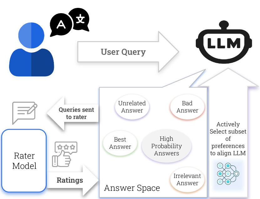
Figure 1: Overview of the Active Multi-Preference Optimization framework. Given a query, the LLM generates diverse responses, which are evaluated by a rater model. Selected responses with different ratings and semantics are then used to train and align the LLM through preference optimization. Active selection of the preferences to optimize over improves training dynamics.

Preference Optimization (PO) has become a standard approach for aligning large language models (LLMs) with human preferences (Christiano et al., 2017; Ouyang et al., 2022; Bai et al., 2022). Traditional alignment pipelines typically rely on pairwise or binary preference comparisons, which may not fully capture the subtleties of human judgment (Rafailov et al., 2024; Liu et al., 2024a; Korbak et al., 2023). As a remedy, there is increasing interest in multi-preference methods, which consider entire sets of responses when providing feedback (Cui et al., 2023; Chen et al., 2024a; Gupta et al., 2024b). By learning from multiple “good” and “bad” outputs simultaneously, these approaches deliver richer alignment signals than purely pairwise methods. At the same time, an important trend in alignment is the shift to on-policy or “self-play” data generation, where the policy learns directly from its own distribution of outputs at each iteration (Chen et al., 2024b; Kumar et al., 2024; Wu et al., 2023, 2024). This feedback loop can accelerate convergence ensuring that the training data stays relevant to the model’s behavior.

However, multi-preference alignment faces a serious bottleneck: modern LLMs can easily generate dozens of candidate responses per query, and incorporating all of these into a single training objective can become computationally infeasible (Askell et al., 2021). Many of these sampled responses end up being highly similar or near-duplicates, providing limited additional information for gradient updates (Long et al., 2024). Consequently, naive attempts to process all generated responses cause both memory blow-ups and diminishing returns in training (Dubey et al., 2024). Given these constraints, identifying a small yet highly informative subset of candidate responses is critical for effective multi-preference learning.

One way to conceptualize the problem is through an “island” metaphor (See Figure 1). Consider each prompt’s answer space as a set of semantic islands, where certain clusters of responses (islands) may be exceptionally good (tall peaks) or particularly poor (flat plains). Focusing only on the tallest peaks or the worst troughs can cause the model to overlook crucial middle-ground modes—“islands” that might harbor subtle failure modes or moderate-quality answers. Therefore, an ideal subset selection strategy should cover the landscape of responses by sampling from each island (Yu et al., 2024). In this paper, we show that selecting representatives from all such “islands” is not only about diversity but can also be tied to an optimal way of suppressing undesired modes under a mild Lipschitz assumption (see Section 6).

Fundamentally, the process of deciding which responses deserve feedback naturally evokes the lens of active learning, where we “actively” pick the most informative data samples (Cohn et al., 1996; Ceravolo et al., 2024; Xiao et al., 2023). By selecting a small yet diverse subset of responses, the model effectively creates a curriculum for itself. Rather than passively training on random or exhaustively sampled data, an active learner queries the examples that yield the greatest improvement when labeled. In our context, we actively pick a handful of responses that best illustrate extreme or underexplored behaviors—whether very good, very bad, or semantically distinct (Wu et al., 2023). This helps the model quickly eliminate problematic modes while reinforcing the most desirable responses. Crucially, we remain on-policy: after each update, the newly refined policy generates a fresh batch of responses, prompting another round of active subset selection (Liu et al., 2021).

We propose Active Multi-Preference Optimization (AMPO), a framework that unifies (a) on-policy data generation, (b) group-based preference learning, and (c) active subset selection. Specifically, we adopt a reference-free group-contrastive objective known as Refa (Gupta et al., 2024a), which jointly leverages multiple “positive” and “negative” responses in a single loss term. On top of this, we explore various active selection schemes—ranging from simplest bottom-$K$ ranking (Meng et al., 2024) to coreset-based clustering (Cohen-Addad et al., 2021, 2022; Huang et al., 2019) and a more theoretically grounded “Opt-Select” method that ties coverage to maximizing expected reward. Our contributions are: (i) a unifying algorithmic pipeline for multi-preference alignment with active selection, (ii) theoretical results demonstrating that coverage of distinct clusters à la k-medoids, can serve as an optimal negative-selection strategy, and (iii) empirical evaluations showing that Ampo achieves state of the art results compared to strong alignment baselines like Simpo. Altogether, we hope this approach advances the state of multi-preference optimization, enabling models to learn more reliably from diverse sets of model behaviors.

Related Works:

We provide a detailed description of our related work in Appendix A covering other multi-preference optimization methods, on-policy alignment, coverage-based selection approaches.

1.1 Our Contributions

• Algorithmic Novelty: We propose Active Multi-Preference Optimization (Ampo), an on-policy framework that blends group-based preference alignment with active subset selection without exhaustively training on all generated responses. This opens out avenues for research on how to select for synthetic data, as we outline in Sections 4 and 8.

• Theoretical Insights: Under mild Lipschitz assumptions, we show that coverage-based negative selection can systematically suppress low-reward modes and maximizes expected reward. This analysis (in Sections 5 and 6) connects our method to the weighted $k$-medoids problem, yielding performance guarantees for alignment.

• State-of-the-Art Results: Empirically, Ampo sets a new benchmark on AlpacaEval with Llama 8B, surpassing strong baselines like Simpo by focusing on a small but strategically chosen set of responses each iteration (see Section 7.1).

• Dataset Releases: We publicly release our AMPO-Coreset-Selection and AMPO-Opt-Selection datasets on Hugging Face. These contain curated response subsets for each prompt, facilitating research on multi-preference alignment.

2 Notations and Preliminaries

We focus on aligning a policy model to human preferences in a single-round (one-shot) scenario. Our goal is to generate multiple candidate responses for each prompt, then actively select a small, high-impact subset for alignment via a group-contrastive objective.

Queries and Policy.

Let $\mathcal{D}=\{x_{1},x_{2},\ldots,x_{M}\}$ be a dataset of $M$ queries (or prompts), each from a larger space $\mathcal{X}$. We have a policy model $P_{\theta}(y\mid x)$, parameterized by $\theta$, which produces a distribution over possible responses $y\in\mathcal{Y}$. To generate diverse answers, we sample from $P_{\theta}(y\mid x)$ at some fixed temperature (e.g., $0.8$). Formally, for each $x_{i}$, we draw up to $N$ responses,

$$\{y_{i,1},y_{i,2},\dots,y_{i,N}\},$$ (1)

from $P_{\theta}(y\mid x_{i})$. Such an on-policy sampling, ensures, we are able to provide preference feedback on queries that are chosen by the model.

For simplicity of notation, we shall presently consider a single query (prompt) $x$ and sampled responses $\{y_{1},\dots,y_{N}\}$ from $P_{\theta}(\cdot\mid x)$, from the autoregressive language model.

Each response $y_{i}$ is assigned a scalar reward

$$r_{i}\;=\;\mathcal{R}(x,\,y_{i})\;\in\;[0,1],$$ (2)

where $\mathcal{R}$ is a fixed reward function or model (not optimized during policy training). We also embed each response via $\mathbf{e}_{i}=\mathcal{E}(y_{i})\in\mathbb{R}^{d}$, where $\mathcal{E}$ might be any sentence or document encoder capturing semantic or stylistic properties.

Although one could train on all $N$ responses, doing so is often computationally expensive. We therefore select a subset $\mathcal{S}\subset\{1,\dots,N\}$ of size $\lvert\mathcal{S}\rvert=K<N$ by maximizing some selection criterion (e.g. favoring high rewards, broad coverage in embedding space, or both). Formally,

$$\mathcal{S}\;=\;\arg\max_{\begin{subarray}{c}\mathcal{I}\subset\{1,\dots,N\}\\ \lvert\mathcal{I}\rvert=K\end{subarray}}\,\mathcal{U}\Bigl{(}\{y_{i}\}_{i\in\mathcal{I}},\,\{r_{i}\}_{i\in\mathcal{I}},\,\{\mathbf{e}_{i}\}_{i\in\mathcal{I}}\Bigr{)},$$ (3)

where $\mathcal{U}$ is a utility function tailored to emphasize extremes, diversity, or other alignment needs.

Next, we split $\mathcal{S}$ into a positive set $\mathcal{S}^{+}$ and a negative set $\mathcal{S}^{-}$. For example, let

$$\overline{r}\;=\;\frac{1}{K}\,\sum_{i\in\mathcal{S}}\,r_{i}$$

be the average reward of the chosen subset, and define

$$\mathcal{S}^{+}\;=\;\{\,i\in\mathcal{S}\,\mid\,r_{i}>\overline{r}\},\quad\mathcal{S}^{-}\;=\;\{\,i\in\mathcal{S}\,\mid\,r_{i}\leq\overline{r}\}.$$

Hence, $\mathcal{S}=\mathcal{S}^{+}\cup\mathcal{S}^{-}$ and $\lvert\mathcal{S}^{+}\rvert+\lvert\mathcal{S}^{-}\rvert=K$.

We train $\theta$ via a reference-free group-contrastive objective known as refa (Gupta et al., 2024a). Concretely, define

$$L_{\text{swepo}}(\theta)\;=\;-\,\log\!\Biggl{(}\!\frac{\displaystyle\sum_{\,i\,\in\,\mathcal{S}^{+}}\;\exp\Bigl{[}s^{\prime}_{\theta}\bigl{(}y_{i}\mid x\bigr{)}\Bigr{]}}{\displaystyle\sum_{\,i\,\in\,(\mathcal{S}^{+}\cup\mathcal{S}^{-})}\;\exp\Bigl{[}s^{\prime}_{\theta}\bigl{(}y_{i}\mid x\bigr{)}\Bigr{]}}\Biggr{)},$$ (4)

where

$$s^{\prime}_{\theta}\bigl{(}y_{i}\mid x\bigr{)}=\log P_{\theta}(y_{i}\mid x)+\alpha\,\bigl{(}r_{i}-\overline{r}\bigr{)}.$$

Here, $P_{\mathrm{ref}}$ is a reference policy (e.g. an older snapshot of $P_{\theta}$ or a baseline model), and $\alpha$ is a hyperparameter scaling the reward difference. In words, swepo encourages the model to increase the log-probability of $\mathcal{S}^{+}$ while decreasing that of $\mathcal{S}^{-}$, all in a single contrastive term that accounts for multiple positives and negatives simultaneously.

Although presented for a single query $x$, this procedure extends straightforwardly to any dataset $\mathcal{D}$ by summing $L_{\text{swepo}}$ across all queries. In subsequent sections, we discuss diverse strategies for selecting $\mathcal{S}$ (and thus $\mathcal{S}^{+}$ and $\mathcal{S}^{-}$), aiming to maximize training efficiency and alignment quality.

3 Algorithm and Methodology

We outline a one-vs-$k$ selection scheme in which a single best response is promoted (positive), while an active subroutine selects $k$ negatives from the remaining $N-1$ candidates. This setup highlights the interplay of three main objectives:

Probability:

High-probability responses under $P_{\theta}(y\mid x)$ can dominate even if suboptimal by reward.

Rewards:

Simply selecting extremes by reward misses problematic ”mediocre” outputs.

Semantics:

Diverse but undesired responses in distant embedding regions must be penalized.

While positives reinforce a single high-reward candidate, active negative selection balances probability, reward and diversity to systematically suppress problematic regions of the response space.

Algorithm. Formally, let $\{y_{1},\dots,y_{N}\}$ be the sampled responses for a single prompt $x$. Suppose we have:
1. A reward function $r_{i}=\mathcal{R}(x,y_{i})\in[0,1]$.
2. An embedding $\mathbf{e}_{i}=\mathcal{E}(y_{i})$.
3. A model probability estimate $\pi_{i}=P_{\theta}(y_{i}\mid x)$.

Selection algorithms may be rating-based selection (to identify truly poor or excellent answers) with coverage-based selection (to explore distinct regions in the embedding space), we expose the model to both common and outlier responses. This ensures that the swepo loss provides strong gradient signals across the spectrum of answers the model is prone to generating. In Algorithm 1, $\textsc{ActiveSelection}(\cdot)$ is a generic subroutine that selects a set of $k$ “high-impact” negatives. We will detail concrete implementations (e.g. bottom-$k$ by rating, clustering-based, etc.) in later sections.

Algorithm 1 Ampo: One-Positive vs. $k$-Active Negatives

1: Input: (1) A set of $N$ responses $\{y_{i}\}$ sampled from $P_{\theta}(y\mid x)$; (2) Their rewards $\{r_{i}\}$, embeddings $\{\mathbf{e}_{i}\}$, and probabilities $\{\pi_{i}\}$; (3) Number of negatives $k$, reference policy $P_{\mathrm{ref}}$, and hyperparameter $\alpha$

2: Output: (i) Positive $y_{+}$; (ii) Negatives $\{y_{j}\}_{j\in S^{-}}$; (iii) Updated parameters $\theta$ via swepo

3: 1. Select One Positive (Highest Reward)

4: $i_{+}\leftarrow\arg\max_{i=1,\dots,N}r_{i}$,  $y_{+}\leftarrow y_{\,i_{+}}$

5: 2. Choose $k$ Negatives via Active Selection

6: $\Omega\leftarrow\{1,\dots,N\}\setminus\{i_{+}\}$

7: $S^{-}\leftarrow\textsc{ActiveSelection}(\Omega,\{r_{i}\},\{\mathbf{e}_{i}\},\{\pi_{i}\},k)$

8: 3. Form One-vs.-$k$ swepo Objective

9: $\overline{r}\leftarrow\frac{r_{\,i_{+}}+\sum_{j\,\in\,S^{-}}r_{j}}{1+k}$

10: For each $y_{i}$:

11: $s^{\prime}_{\theta}(y_{i})=\log P_{\theta}(y_{i}\mid x)+\alpha(r_{i}-\overline{r})$

12: $L_{\text{swepo}}(\theta)=-\log\!\Biggl{(}\frac{\exp\!\bigl{[}s^{\prime}_{\theta}(y_{+})\bigr{]}}{\exp\!\bigl{[}s^{\prime}_{\theta}(y_{+})\bigr{]}+\sum_{\,j\,\in\,S^{-}}\exp\!\bigl{[}s^{\prime}_{\theta}(y_{j})\bigr{]}}\Biggr{)}$

13: 4. Update Model Parameters: $\theta\leftarrow\theta-\eta\,\nabla_{\theta}L_{\text{swepo}}(\theta)$

14: return  The chosen positive $y_{+}$, the negative set $\{y_{j}\}_{j\in S^{-}}$, and the updated parameters $\theta$

3.1 Detailed Discussion of Algorithm 1

The algorithm operates in four key steps: First, it selects the highest-reward response as the positive example (lines 3-4). Second, it actively selects $k$ negative examples by considering their rewards, probabilities $\pi_{i}$, and embedding distances $\mathbf{e}_{i}$ to capture diverse failure modes (lines 5-7). Third, it constructs the swepo objective by computing normalized scores $s^{\prime}_{\theta}$ using the mean reward $\overline{r}$ and forming a one-vs-$k$ contrastive loss (lines 8-12). Finally, it updates the model parameters to increase the probability of the positive while suppressing the selected negatives (line 13). This approach ensures both reinforcement of high-quality responses and systematic penalization of problematic outputs across the response distribution.

4 Active Subset Selection Strategies

In this section, we present two straightforward yet effective strategies for actively selecting a small set of negative responses in the AMPO framework. First, we describe a simple strategy, AMPO-BottomK, that directly picks the lowest-rated responses. Second, we propose AMPO-Coreset, a clustering-based method that selects exactly one negative from each cluster in the embedding space, thereby achieving broad coverage of semantically distinct regions. In Section D, we connect this clustering-based approach to the broader literature on coreset construction, which deals with selecting representative subsets of data.

4.1 AMPO-BottomK

AMPO-BottomK is the most direct approach that we use for comparison: given $N$ sampled responses and their scalar ratings $\{r_{i}\}_{i=1}^{N}$, we simply pick the $k$ lowest-rated responses as negatives. This can be expressed as:

$$S^{-}\;=\;\mathrm{argtopk}_{i}(-\,r_{i},\,k),$$ (5)

which identifies the $k$ indices with smallest $r_{i}$. Although conceptually simple, this method can be quite effective when the reward function reliably indicates “bad” behavior. Furthermore to break-ties, we use minimal cosine similarity with the currently selected set.

4.2 AMPO-Coreset (Clustering-Based Selection)

Ampo-BottomK may overlook problematic modes that are slightly better than the bottom-k, but fairly important to learn on. A diversity-driven approach, which we refer to as Ampo-CoreSet, explicitly seeks coverage in the embedding space by partitioning the $N$ candidate responses into $k$ clusters and then selecting the lowest-rated response within each cluster. Formally:

$$i^{-}_{j}\;=\;\arg\min_{\,i\,\in\,C_{j}}\;r_{i},\,j=1,\dots,k,\,S^{-}\;=\;\bigl{\{}\,i^{-}_{1},\dots,i^{-}_{k}\bigr{\}}$$

where $C_{j}$ is the set of responses assigned to cluster $j$ by a $k$-means algorithm (Har-Peled & Mazumdar 2004; Cohen-Addad et al. 2022; see also Section D). The pseudo-code is provided in Algorithm 2.

Algorithm 2 Ampo-CoreSet via k-means

1: Input:

2: (1) $N$ responses, each with embedding $\mathbf{e}_{i}\in\mathbb{R}^{d}$ and rating $r_{i}$

3: (2) Desired number of negatives $k$

4: 

5: Step 1: Run $k$-means on embeddings

6: Initialize $\{\mathbf{c}_{1},\dots,\mathbf{c}_{k}\}\subset\mathbb{R}^{d}$ (e.g., via $k$-means++)

7: repeat

8:  $\pi(i)=\arg\min_{1\leq j\leq k}\|\mathbf{e}_{i}-\mathbf{c}_{j}\|^{2}$,  $i=1,\dots,N$

9:  $\mathbf{c}_{j}=\frac{\sum_{i:\pi(i)=j}\mathbf{e}_{i}}{\sum_{i:\pi(i)=j}1}$,  $j=1,\dots,k$

10: until convergence

11: 

12: Step 2: In each cluster, pick the bottom-rated response

13: For each $j\in\{1,\dots,k\}$, define $C_{j}=\{\,i\mid\pi(i)=j\}$

14: Then $i_{j}^{-}=\arg\min_{i\in C_{j}}r_{i}$,  $j=1,\dots,k$

15: 

16: Step 3: Return negatives

17: $S^{-}=\{\,i_{1}^{-},\,i_{2}^{-},\dots,i_{k}^{-}\}$

18: return  $S^{-}$ as the set of $k$ negatives

This approach enforces that each cluster—a potential “mode” in the response space—contributes at least one negative example. Hence, AMPO-Coreset can be interpreted as selecting representative negatives from diverse semantic regions, ensuring that the model is penalized for a wide variety of undesired responses.

5 Opt-Select: Active Subset Selection by Optimizing Expected Reward

In this section, we propose Opt-Select: a strategy for choosing $k$ negative responses (plus one positive) so as to maximize the policy’s expected reward under a Lipschitz continuity assumption. Specifically, we model the local “neighborhood” influence of penalizing each selected negative and formulate an optimization problem that seeks to suppress large pockets of low-reward answers while preserving at least one high-reward mode. We first describe the intuition and objective, then present two solution methods: a mixed-integer program (MIP) and a local search approximation.

5.1 Lipschitz-Driven Objective

Let $\{y_{i}\}_{i=1}^{n}$ be candidate responses sampled on-policy, each with reward $r_{i}\in[0,1]$ and embedding $\mathbf{e}_{i}\in\mathbb{R}^{d}$. Suppose that if we completely suppress a response $y_{j}$ (i.e. set its probability to zero), all answers within distance $\|\mathbf{e}_{i}-\mathbf{e}_{j}\|$ must also decrease in probability proportionally, due to a Lipschitz constraint on the policy. Concretely, if the distance is $d_{i,j}=\|\mathbf{e}_{i}-\mathbf{e}_{j}\|$, and the model’s Lipschitz constant is $L$, then the probability of $y_{i}$ cannot remain above $L\,d_{i,j}$ if $y_{j}$ is forced to probability zero.

From an expected reward perspective, assigning zero probability to low-reward responses (and their neighborhoods) improves overall alignment. To capture this rigorously, observe that the penalty from retaining a below-average answer $y_{i}$ can be weighted by:

$$w_{i}\;=\;\exp\bigl{(}\,\overline{r}\;-\;r_{i}\bigr{)},$$ (6)

where $\overline{r}$ is (for instance) the mean reward of $\{r_{i}\}$. Intuitively, $w_{i}$ is larger for lower-reward $y_{i}$, indicating it is more harmful to let $y_{i}$ and its neighborhood remain at high probability.

Next, define a distance matrix

$$A_{i,j}\;=\;\bigl{\|}\mathbf{e}_{i}-\mathbf{e}_{j}\bigr{\|}_{2},\quad 1\leq i,j\leq n.$$ (7)

Selecting a subset $S\subseteq\{1,\dots,n\}$ of “negatives” to penalize suppresses the probability of each $i$ in proportion to $\min_{j\in S}A_{i,j}$. Consequently, a natural cost function measures how much “weighted distance” $y_{i}$ has to its closest chosen negative:

$$\text{Cost}(S)\;=\;\sum_{i=1}^{n}w_{i}\;\min_{\,j\in S}\;A_{i,j}.$$ (8)

Minimizing equation 8 yields a subset $S$ of size $k$ that “covers” or “suppresses” as many low-reward responses (large $w_{i}$) as possible. We then add one positive index $i_{\mathrm{top}}$ with the highest $r_{i}$ to amplify a top-quality answer. This combination of one positive plus $k$ negatives provides a strong signal in the training loss.

Interpretation and Connection to Weighted k-medoids.

If each negative $j$ “covers” responses $i$ within some radius (or cost) $A_{i,j}$, then equation 8 is analogous to a weighted $k$-medoid objective, where we choose $k$ items (negatives) to minimize a total weighted distance. Formally, this can be cast as a mixed-integer program (MIP) (Problem 9 below). For large $n$, local search offers an efficient approximation.

5.2 Mixed-Integer Programming Formulation

Define binary indicators $x_{j}=1$ if we choose $y_{j}$ as a negative, and $z_{i,j}=1$ if $i$ is assigned to $j$ (i.e. $\min_{j\in S}A_{i,j}$ is realized by $j$). We write:

$$\textbf{Problem }\mathcal{P}:\quad \min_{\begin{subarray}{c}x_{j}\in\{0,1\},\ z_{i,j}\in\{0,1\},\ y_{i}\geq 0\end{subarray}}\sum_{i=1}^{n}w_{i}\,y_{i}$$ (9)

s.t. $$\sum_{j=1}^{n}x_{j}=k,z_{i,j}\leq x_{j},\sum_{j=1}^{n}z_{i,j}=1,\forall\,i,$$

$$y_{i}\leq A_{i,j}+M\,(1-z_{i,j}),$$

$$y_{i}\geq A_{i,j}-M\,(1-z_{i,j}),\quad\forall\,i,j,$$ (10)

where $M=\max_{i,j}A_{i,j}$. In essence, each $i$ is forced to assign to exactly one chosen negative $j$, making $y_{i}=A_{i,j}$, i.e. the distance between the answer embeddings for answer $\{i,j\}$. Minimizing $\sum_{i}w_{i}\,y_{i}$ (i.e. equation 8) then ensures that low-reward points ($w_{i}$ large) lie close to at least one penalized center.

Algorithmic Overview.

Solving $\mathcal{P}$ gives the $k$ negatives $S_{\mathrm{neg}}$, while the highest-reward index $i_{\mathrm{top}}$ is chosen as a positive. The final subset $\{i_{\mathrm{top}}\}\cup S_{\mathrm{neg}}$ is then passed to the swepo loss (see Section 3). Algorithm 3 outlines the procedure succinctly.

Algorithm 3 Ampo-OptSelect via Solving MIP

1: Input: Candidates $\{y_{i}\}_{i=1}^{n}$ with $r_{i},\mathbf{e}_{i}$; integer $k$

2: Compute $i_{\mathrm{top}}=\arg\max_{i}\,r_{i}$

3: Let $w_{i}=\exp(\,\overline{r}-r_{i})$ with $\overline{r}$ as mean reward

4: Solve Problem equation 9 to get $\{x_{j}^{*}\},\{z_{i,j}^{*}\},\{y_{i}^{*}\}$

5: Let $S_{\mathrm{neg}}=\{\,j\mid x_{j}^{*}=1\}$ (size $k$)

6: return  $\{\,i_{\mathrm{top}}\}\cup S_{\mathrm{neg}}$ for swepo training

5.3 Local Search Approximation

For large $n$, an exact MIP can be expensive. A simpler local search approach initializes a random subset $S$ of size $k$ and iteratively swaps elements in and out if it lowers the cost equation 8. In practice, this provides an efficient approximation, especially when $n$ or $k$ grows.

Algorithm 4 Ampo-OptSelect via Coordinate Descent

1: Input: Set $I=\{1,\dots,n\}$, integer $k$, distances $A_{i,j}$, rewards $\{r_{i}\}$

2: Find $i_{\mathrm{top}}=\arg\max_{i}\,r_{i}$

3: Compute $w_{i}=\exp(\,\overline{r}-r_{i})$ and $d_{i,j}=A_{i,j}$

4: Initialize a random subset $S\subseteq I\setminus\{i_{\mathrm{top}}\}$ of size $k$

5: while improving do

6:  Swap $j_{\mathrm{out}}\in S$ with $j_{\mathrm{in}}\notin S$ if it decreases $\sum_{i\in I}w_{i}\,\min_{j\in S}d_{i,j}$

7: end while

8: return  $S_{\mathrm{neg}}=S$ (negatives) and $i_{\mathrm{top}}$ (positive)

Intuition.

If $y_{i}$ is far from all penalized points $j\in S$, then it remains relatively “safe” from suppression, which is undesirable if $r_{i}$ is low (i.e. $w_{i}$ large). By systematically choosing $S$ to reduce $\sum_{i}w_{i}\,\min_{j\in S}d_{i,j}$, we concentrate penalization on high-impact, low-reward regions. The local search repeatedly swaps elements until no single exchange can further reduce the cost.

5.4 Why “Opt-Select”? A Lipschitz Argument for Expected Reward

We name the procedure “Opt-Select” because solving equation 9 (or its local search variant) directly approximates an optimal subset for improving the policy’s expected reward. Specifically, under a Lipschitz constraint with constant $L$, assigning zero probability to each chosen negative $y_{j}$ implies neighboring answers $y_{i}$ at distance $d_{i,j}$ cannot exceed probability $L\,d_{i,j}$. Consequently, their contribution to the “bad behavior” portion of expected reward is bounded by

$$\exp\bigl{(}r_{\max}-r_{i}\bigr{)}\,\bigl{(}\,L\,d_{i,j}\bigr{)},$$

where $r_{\max}$ is the rating of the best-rated response. Dividing by a normalization factor (such as $\exp(r_{\max}-\overline{r})\,L$), one arrives at a cost akin to $w_{i}\,d_{i,j}$ with $w_{i}=\exp(\overline{r}-r_{i})$. This aligns with classical min-knapsack of minimizing some costs subject to some constraints, and has close alignment with the weighted $k$-medoid notions of “covering” important items at minimum cost.

6 Theoretical Results: Key Results

In this section, we present the core theoretical statements used throughout the paper. Full extended proofs appear in Appendices B–D.

6.1 Setup and Assumptions

(A1) $L$-Lipschitz Constraint.

When a response $y_{j}$ is penalized (probability $p_{j}=0$), any other response $y_{i}$ within embedding distance $A_{i,j}$ must satisfy $p_{i}\leq L\,A_{i,j}$.

(A2) Single Positive Enforcement.

We allow one highest-reward response $y_{i_{\mathrm{top}}}$ to be unconstrained, i.e. $p_{i_{\mathrm{top}}}$ is not pulled down by the negatives.

(A3) Finite Support.

We focus on a finite set of $n$ candidate responses $\{y_{1},\dots,y_{n}\}$ and their scalar rewards $\{r_{i}\}$, each embedded in $\mathbb{R}^{d}$ with distance $A_{i,j}=\|\mathbf{e}_{i}-\mathbf{e}_{j}\|$.

6.2 Optimal Negatives via Coverage

Theorem 6.1 (Optimality of Opt-Select).

Under assumptions (A1)–(A3), let $\mathcal{S}^{*}$ be the set of $k$ “negative” responses that minimizes the coverage cost

$$\mathrm{Cost}(\mathcal{S})\;=\;\sum_{i=1}^{n}\exp(\,\overline{r}-r_{i})\;\min_{j\in\mathcal{S}}A_{i,j},$$ (11)

where $\overline{r}$ is a reference reward (e.g. average of $\{r_{i}\}$). Then $\mathcal{S}^{*}$ also maximizes the expected reward among all Lipschitz-compliant policies of size $k$ (with a single positive). Consequently, selecting $\mathcal{S}^{*}$ and allowing $p_{i_{\mathrm{top}}}\approx 1$ is optimal.

Sketch of Proof.

(See Appendix B for details.) We show a one-to-one correspondence between minimizing coverage cost $\sum_{i}w_{i}\min_{j\in\mathcal{S}}A_{i,j}$ and maximizing the feasible expected reward $\sum_{i}r_{i}p_{i}$ under the Lipschitz constraint. Low-reward responses with large $w_{i}$ must lie close to at least one negative $j\in\mathcal{S}$; otherwise, they are not sufficiently suppressed. A mixed-integer program encodes this cost explicitly, and solving it yields the unique $\mathcal{S}^{*}$ that maximizes reward.

6.3 Local Search for Weighted $k$-Medoids

(A4) Weighted $k$-Medoids Setup.

We have $n$ points $\{1,\dots,n\}$ in a metric space with distance $d(\cdot,\cdot)\geq 0$, each with weight $w_{i}\geq 0$. Our goal is to find a subset $\mathcal{S}$ of size $k$ minimizing

$$\mathrm{Cost}(\mathcal{S})\;=\;\sum_{i=1}^{n}w_{i}\,\min_{j\in\mathcal{S}}d(i,j).$$

Theorem 6.2 (Local Search Approximation).

Suppose we apply a $1$-swap local search algorithm to select $k$ medoids. Let $\widehat{\mathcal{S}}$ be the resulting local optimum and let $\mathcal{S}^{*}$ be the globally optimal subset. Then

$$\mathrm{Cost}\bigl{(}\widehat{\mathcal{S}}\bigr{)}\;\leq\;5\,\times\,\mathrm{Cost}\bigl{(}\mathcal{S}^{*}\bigr{)}.$$

The running time is polynomial in $n$ and $k$.

Sketch of Proof.

(See Appendix C for a complete proof.) Assume by contradiction that $\mathrm{Cost}(\widehat{\mathcal{S}})>5\,\mathrm{Cost}(\mathcal{S}^{*})$. We then show there exists a profitable swap (removing some $j\in\widehat{\mathcal{S}}$ and adding $j^{*}\in\mathcal{S}^{*}$) that strictly decreases cost, contradicting the local optimality of $\widehat{\mathcal{S}}$.

6.4 Coreset and Bounded Intra-Cluster Distance

(A5) Bounded-Diameter Clusters.

We assume $k$ clusters of diameter at most $d_{\max}$ in Ampo-CoreSet.

Theorem 6.3 (Distribution-Dependent Coreset Guarantee).

Suppose we form $k$ clusters each of diameter $\leq d_{\max}$ in an embedding space $\mathbb{R}^{d}$, and from each cluster we pick one response as a “negative.” Under a Lipschitz constant $L$, this subset induces $p_{i}\leq L\,d_{\max}$ for all $i$ in each cluster. With sufficiently many samples (drawn from a distribution of prompts/responses), with probability at least $1-\delta$, for a $(1-\delta)$ fraction of new draws, the resulting Lipschitz-compliant policy is within a factor $(1\pm\varepsilon)$ of the optimal $k$-subset solution.

Sketch of Proof.

(See Appendix D.) By choosing one representative from each of $k$ bounded-diameter clusters, we ensure that all similar (i.e. same-cluster) responses are suppressed. A uniform convergence argument shows that, with enough sampled data, responses from the same distribution are close to one of the clusters, guaranteeing approximate coverage and thus near-optimal expected reward.

Method	AlpacaEval 2		Arena-Hard	MT-Bench
	LC (%)	WR (%)	WR (%)	GPT-4
Base	28.4	28.4	26.9	7.93
Best-vs-worst (Simpo)	47.6	44.7	34.6	7.51
Ampo-Bottomk	50.8	50.5	35.3	8.11
Ampo-Coreset	52.4	52.1	39.4	8.12
Ampo-Opt-Select	51.6	51.2	37.9	7.96

Table 1: Comparison of various preference optimization baselines on AlpacaEval, Arena-Hard, and MT-Bench benchmarks for Llama-3-Instruct (8B). LC-WR represents length-controlled win rate, and WR represents raw win rate. Best results are in bold, second-best are underlined. Our method (Ampo) achieves SOTA performance across all metrics, with different variants achieving either best or second-best results consistently.

7 Experiments

7.1 Experimental Setup

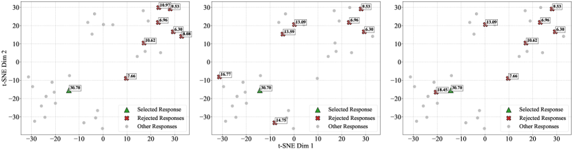
Figure 2: t-SNE visualization of projected high-dimensional response embeddings into a 2D space, illustrating the separation of actively selected responses. (a) AMPO-BottomK (baseline). (b) AMPO-Coreset (ours). (c) Opt-Select (ours). We see that the traditional baselines select many responses close to each other, based on their rating. This provides insufficient feedback to the LLM during preference optimization. In contrast, our methods simultaneously optimize for objectives including coverage, generation probability as well as preference rating.

Model and Training Settings:

For our experiments, we utilize a pretrained instruction-tuned model (meta-llama/MetaLlama-3-8B-Instruct), as the SFT model. These models have undergone extensive instruction tuning, making them more capable and robust compared to the SFT models used in the Base setup. However, their reinforcement learning with human feedback (RLHF) procedures remain undisclosed, making them less transparent.

To reduce distribution shift between the SFT models and the preference optimization process, we follow the approach in (Tran et al., 2023) and generate the preference dataset using the same SFT models. This ensures that our setup is more aligned with an on-policy setting. Specifically, we utilize prompts from the UltraFeedback dataset (Cui et al., 2023) and regenerate the resonses using the SFT models. For each prompt x, we produce 32 responses by sampling from the SFT model with a sampling temperature of 0.8. We then use the reward model (Skywork/Skywork-Reward-Llama-3.1-8B-v0.2) (Liu et al., 2024b) to score all the 32 responses. Then the response are selected based on the Active Subset selection strategies a.) AMPO-Bottomk b.) AMPO-Coreset c.) AMPO-OptSelect

In our experiments, we observed that tuning hyperparameters is critical for optimizing the performance . Carefully selecting hyperparameter values significantly impacts the effectiveness of these methods across various datasets.We found that setting the $\beta$ parameter in the range of 5.0 to 10.0 consistently yields strong performance, while tuning the $\gamma$ parameter within the range of 2 to 4 further improved performance. These observations highlight the importance of systematic hyperparameter tuning to achieve reliable outcomes across diverse datasets.

Evaluation Benchmarks

We evaluate our models using three widely recognized open-ended instruction-following benchmarks: MT-Bench (Zheng et al., 2023), AlpacaEval2 (Dubois et al., 2024), and Arena-Hard v0.1. These benchmarks are commonly used in the community to assess the conversational versatility of models across a diverse range of queries.

AlpacaEval 2 comprises 805 questions sourced from five datasets, while MT-Bench spans eight categories with a total of 80 questions. The recently introduced Arena-Hard builds upon MT-Bench, featuring 500 well-defined technical problem-solving queries designed to test more advanced capabilities.

We adhere to the evaluation protocols specific to each benchmark when reporting results. For AlpacaEval 2, we provide both the raw win rate (WR) and the length-controlled win rate (LC), with the latter being designed to mitigate the influence of model verbosity. For Arena-Hard, we report the win rate (WR) against a baseline model. For MT-Bench, we present the scores as evaluated by GPT-4-Preview-1106, which serve as the judge model.

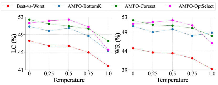
Figure 3: Effect of Sampling Temperature on different baselines for on the AlpacaEval 2 Benchmark: (a) Length-Controlled Win Rate (LC) and (b) Overall Win Rate (WR).

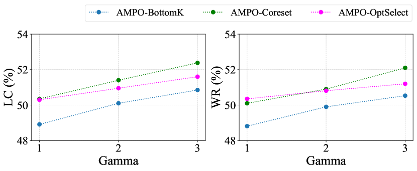
Figure 4: Effect of Gamma on AlpacaEval2 for Active Subset Selection Strategies.

7.2 Experimental Result

Impact of Selection Strategies on Diversity.

Figure 2 shows a t-SNE projection of response embeddings, highlighting how each selection method samples the answer space:
AMPO-BottomK: Tends to pick a tight cluster of low-rated responses, limiting coverage and redundancy in feedback.
AMPO-Coreset: Uses coreset-based selection to cover more diverse regions, providing coverage of examples.
Opt-Select: Further balances reward extremity, and embedding coverage, yielding well-separated response clusters and more effective supervision for preference alignment.

Key analysis from Fig. 2 demonstrate that our selection strategies significantly improve response diversity compared to traditional baselines. By actively optimizing for coverage-aware selection, our methods mitigate redundancy in selected responses, leading to better preference modeling and enhanced LLM alignment.

Impact of Temperature Sampling for Different Active Selection Approaches

To analyze the impact of temperature-controlled response sampling on different active selection approaches, we conduct an ablation study by varying the sampling temperature from 0 to 1.0 in increments of 0.25 on AlpacaEval2 benchmark as demonstrated in Figure 3. We evaluate our active selection strategies observe a general trend of declining performance with increasing temperature. Key observation: Ampo-Coreset and Ampo-OptSelect demonstrate robustness to temperature variations, whereas WR-SimPO and bottom-k selection are more sensitive.

Effect of gamma for Active Selection Approaches

To further investigate the sensitivity of core-set selection to different hyper-parameter settings, we conduct an ablation study on the impact of varying the gamma parameter as show in Figure 4. As gamma increases from 1 to 3, we observe a consistent improvement in both LC-WR and WR scores. Key findings highlight the importance of tuning gamma appropriately to maximize the effectiveness of active-selection approaches.

8 Discussion & Future Work

Iteration via Active Synthetic Data Generation.

When we combine reward signals and output-embedding signals in active sampling, we naturally create a pathway to synthetic data creation. Through multi-preference optimization on diverse queries, the model continually improves itself by receiving feedback on different modes of failure (and success). Crucially, because this process is on-policy, the model directly surfaces new candidate answers for which it is most uncertain or prone to errors. The selection for coverage ensures that we efficiently address a large portion of the measurable answer space, rather than merely focusing on obvious or extreme failures.

Over multiple epochs, such a growing corpus of synthetic data can be used to refine or re-check the reward model, establishing a feedback loop between policy improvement and reward-model improvement. We believe this to be an important direction of future work.

Impact Statement

This paper presents work whose goal is to advance the field of Machine Learning. There are many potential societal consequences of our work, none which we feel must be specifically highlighted here.

 

Supplementary Materials

 

These supplementary materials provide additional details, derivations, and experimental results for our paper. The appendix is organized as follows:

• Section A provides a more comprehensive overview of the related literature.

• Section B provides theoretical analysis of the equivalence of the optimal selection integer program and the reward maximization objective.

• Section C shows a constant factor approximation for the coordinate descent algorithm in polynomial time.

• Section D provides theoretical guarantees for our k-means style coreset selection algorithm.

• Section E provides the code for computation of the optimal selection algorithm.

• Section F provides t-sne plots for the various queries highlighting the performance of our algorithms.

Appendix A Related Work

Preference Optimization in RLHF.

Direct Preference Optimization (DPO) is a collection of techniques for fine-tuning language models based on human preferences (Rafailov et al., 2024). Several variants of DPO have been developed to address specific challenges and improve its effectiveness (Ethayarajh et al., 2024; Zeng et al., 2024; Dong et al., 2023; Yuan et al., 2023). For example, KTO and TDPO focus on different aspects of preference optimization, while RAFT and RRHF utilize alternative forms of feedback. Other variants, such as SPIN, CPO, ORPO, and SimPO, introduce additional objectives or regularizations to enhance the optimization process (Chen et al., 2024b; Xu et al., 2024; Hong et al., 2024; Meng et al., 2024).

Further variants, including R-DPO, LD-DPO, sDPO, IRPO, OFS-DPO, and LIFT-DPO, address issues like length bias, training strategies, and specific reasoning tasks. These diverse approaches demonstrate the ongoing efforts to refine and enhance DPO, addressing its limitations and expanding its applicability to various tasks and domains (Park et al., 2024; Liu et al., 2024c; Pang et al., 2024; Qi et al., 2024; Yuan et al., 2024).

Multi-Preference Approaches.

Recent work extends standard RLHF to consider entire sets of responses at once, enabling more nuanced feedback signals (Rafailov et al., 2024; Cui et al., 2023; Chen et al., 2024a). Group-based objectives capture multiple acceptable (and multiple undesirable) answers for each query, rather than only a single “better vs. worse” pair. Gupta et al. (2024b) propose a contrastive formulation, Swepo, that jointly uses multiple “positives” and “negatives.” Such multi-preference methods can reduce label noise and better reflect the complexity of real-world tasks, but their computational cost grows if one attempts to incorporate all generated outputs (Cui et al., 2023; Chen et al., 2024a).

On-Policy Self-Play.

A key advancement in reinforcement learning has been self-play or on-policy generation, where the model continuously updates and re-generates data from its own evolving policy (Silver et al., 2016, 2017). In the context of LLM alignment, on-policy sampling can keep the training set aligned with the model’s current distribution of outputs (Christiano et al., 2017; Wu et al., 2023). However, this approach can significantly inflate the number of candidate responses, motivating the need for selective down-sampling of training examples.

Active Learning for Policy Optimization.

The notion of selectively querying the most informative examples is central to active learning (Cohn et al., 1996; Settles, 2009), which aims to reduce labeling effort by focusing on high-utility samples. Several works incorporate active learning ideas into reinforcement learning, e.g., uncertainty sampling or diversity-based selection (Sener & Savarese, 2017; Zhang et al., 2022). In the RLHF setting, Christiano et al. (2017) highlight how strategic feedback can accelerate policy improvements, while others apply active subroutines to refine reward models (Wu et al., 2023). By picking a small yet diverse set of responses, we avoid both computational blow-ups and redundant training signals.

Clustering and Coverage-Based Selection.

Selecting representative subsets from a large dataset is a classic problem in machine learning and combinatorial optimization. Clustering techniques such as $k$-means and $k$-medoids (Hartigan & Wong, 1979) aim to group points so that distances within each cluster are small. In the RLHF context, embedding model outputs and clustering them can ensure coverage over semantically distinct modes (Har-Peled & Mazumdar, 2004; Cohen-Addad et al., 2022). These methods connect to the facility location problem (Oh Song et al., 2017)—minimizing the cost of “covering” all points with a fixed number of centers—and can be addressed via coreset construction (Feldman, 2020).

Min-Knapsack and Integer Programming.

When picking a subset of size $k$ to cover or suppress “bad” outputs, one may cast the objective in a min-knapsack or combinatorial optimization framework (Kellerer et al., 2004a). For instance, forcing certain outputs to zero probability can impose constraints that ripple to nearby points in embedding space, linking coverage-based strategies to integer programs (Chen et al., 2020). Cohen-Addad et al. (2022) and Har-Peled & Mazumdar (2004) demonstrate how approximate solutions to such subset selection problems can achieve strong empirical results in high-dimensional scenarios. By drawing from these established concepts, our method frames the selection of negative samples in a Lipschitz coverage sense, thereby enabling both theoretical guarantees and practical efficiency in multi-preference alignment.

Collectively, our work stands at the intersection of multi-preference alignment (Gupta et al., 2024b; Cui et al., 2023), on-policy data generation (Silver et al., 2017; Ouyang et al., 2022), and active learning (Cohn et al., 1996; Settles, 2009). We leverage ideas from clustering (k-means, k-medoids) and combinatorial optimization (facility location, min-knapsack) (Kellerer et al., 2004b; Cacchiani et al., 2022) to construct small yet powerful training subsets that capture both reward extremes and semantic diversity. The result is an efficient pipeline for aligning LLMs via multi-preference signals without exhaustively processing all generated responses.

Appendix B Extended Theoretical Analysis of Opt-Select

In this appendix, we present a more detailed theoretical treatment of Ampo-OptSelect. We restate the core problem setup and assumptions, then provide rigorous proofs of our main results. Our exposition here augments the concise version from the main text.

B.1 Problem Setup

Consider a single prompt (query) $x$ for which we have sampled $n$ candidate responses $\{\,y_{1},\,y_{2},\,\ldots,\,y_{n}\}$. Each response $y_{i}$ has:

• A scalar reward $r_{i}\in[0,1]$.

• An embedding $\mathbf{e}_{i}\in\mathbb{R}^{d}.$

We define the distance between two responses $y_{i}$ and $y_{j}$ by

$$A_{i,j}\;=\;\|\mathbf{e}_{i}\,-\,\mathbf{e}_{j}\|.$$ (12)

We wish to learn a policy $\{p_{i}\}$, where $p_{i}\geq 0$ and $\sum_{i=1}^{n}p_{i}=1$. The policy’s expected reward is

$$\mathrm{ER}(p)\;=\;\sum_{i=1}^{n}r_{i}\,p_{i}.$$ (13)

Positive and Negative Responses.

We designate exactly one response, denoted $y_{i_{\mathrm{top}}}$, as a positive (the highest-reward candidate). All other responses are potential “negatives.” Concretely:

• We fix one index $i_{\mathrm{top}}$ with $\displaystyle i_{\mathrm{top}}\;=\;\arg\max_{i\in\{1,\dots,n\}}\,r_{i}.$

• We choose a subset $\mathcal{S}\subseteq\{1,\dots,n\}\setminus\{i_{\mathrm{top}}\}$ of size $k$, whose elements are forced to have $p_{j}=0$. (These are the “negatives.”)

B.1.1 Lipschitz Suppression Constraint

We assume a mild Lipschitz-like rule:

1. $L$-Lipschitz Constraint. If $p_{j}=0$ for some $j\in\mathcal{S}$, then for every response $y_{i}$, we must have

   $$p_{i}\;\leq\;L\,A_{i,j}\;=\;L\,\|\mathbf{e}_{i}\,-\,\mathbf{e}_{j}\|.$$ (14)

The effect is that whenever we force a particular negative $j$ to have $p_{j}=0$, any response $i$ near $j$ in embedding space also gets pushed down, since $p_{i}\leq L\,A_{i,j}$. By selecting a set of $k$ negatives covering many “bad” or low-reward regions, we curb the policy’s probability of generating undesirable responses.

Goal.

Define the feasible set of distributions:

$$\mathcal{F}(\mathcal{S})\;=\;\Bigl{\{}\,\{p_{i}\}\colon p_{j}=0\ \forall\,j\in\mathcal{S},\ p_{i}\leq L\,\min_{j\in\mathcal{S}}A_{i,j}\ \forall\,i\notin\{\,i_{\mathrm{top}}\}\cup\mathcal{S}\Bigr{\}}.$$ (15)

We then have a two-level problem:

$$\max_{\,\begin{subarray}{c}\mathcal{S}\,\subseteq\{1,\dots,n\}\setminus\{i_{\mathrm{top}}\}\\ |\mathcal{S}|=k\end{subarray}}\quad\max_{\begin{subarray}{c}\{p_{i}\}\in\mathcal{F}(\mathcal{S})\\ \sum_{i}p_{i}=1,\;p_{i}\geq 0\end{subarray}}\quad\sum_{i=1}^{n}r_{i}\,p_{i},$$

$$\text{subject to}\quad p_{i_{\mathrm{top}}}\text{ is unconstrained (no Lipschitz bound).}$$ (16)

We seek $\mathcal{S}$ that maximizes the best possible Lipschitz-compliant expected reward.

B.2 Coverage View and the MIP Formulation

Coverage Cost.

To highlight the crucial role of “covering” low-reward responses, define a weight

$$w_{i}\;=\;\exp\bigl{(}\,\overline{r}-r_{i}\bigr{)},$$ (17)

where $\overline{r}$ can be, for instance, the average reward $\frac{1}{n}\sum_{i=1}^{n}r_{i}$. Then a natural coverage cost is

$$\mathrm{Cost}(\mathcal{S})\;=\;\sum_{i=1}^{n}w_{i}\,\min_{j\in\mathcal{S}}A_{i,j}.$$ (18)

A small $\min_{j\in\mathcal{S}}A_{i,j}$ means response $i$ is “close” to at least one negative center $j$. If $r_{i}$ is low, then $w_{i}$ is large, so we put higher penalty on leaving $i$ uncovered. Minimizing $\mathrm{Cost}(\mathcal{S})$ ensures that important (low-reward) responses are forced near penalized centers, thus suppressing them in the policy distribution.

MIP $\mathcal{P}$ for Coverage Minimization.

We can write a mixed-integer program:

$$\textbf{Problem }\mathcal{P}:\; \min_{\,\begin{subarray}{c}x_{j}\in\{0,1\}\\ z_{i,j}\in\{0,1\}\\ y_{i}\geq 0\end{subarray}}\sum_{i=1}^{n}w_{i}\,y_{i},$$

$$\text{subject to}\begin{cases}\displaystyle\sum_{j=1}^{n}x_{j}=k,\\[1.99997pt] z_{i,j}\leq x_{j},\quad\sum_{j=1}^{n}z_{i,j}=1,\quad\forall\,i,\\[1.99997pt] y_{i}\leq A_{i,j}+M\,(1-z_{i,j}),\\[1.99997pt] y_{i}\geq A_{i,j}-M\,(1-z_{i,j}),\quad\forall\,i,j,\end{cases}$$ (19)

where $M=\max_{i,j}A_{i,j}$. Intuitively, each $x_{j}$ indicates if $j$ is chosen as a negative; each $z_{i,j}$ indicates whether $i$ is “assigned” to $j$. At optimality, $y_{i}=\min_{j\in\mathcal{S}}A_{i,j}$, so the objective $\sum_{i}w_{i}\,y_{i}$ is precisely $\mathrm{Cost}(\mathcal{S})$. Hence solving $\mathcal{P}$ yields $\mathcal{S}^{*}$ that minimizes coverage cost equation 18.

B.3 Key Lemma: Equivalence of Coverage Minimization and Lipschitz Suppression

Lemma B.1 (Coverage $\Leftrightarrow$ Suppression).

Assume (A1) (the $L$-Lipschitz constraint, equation 14) and let $i_{\mathrm{top}}$ be a highest-reward index. Suppose $\mathcal{S}\subseteq\{1,\dots,n\}\setminus\{i_{\mathrm{top}}\}$ is a subset of size $k$. Then:

1. Choosing $\mathcal{S}$ that minimizes $\mathrm{Cost}(\mathcal{S})$ yields the strongest suppression of low-reward responses and thus the best possible feasible expected reward under the Lipschitz constraint.

2. Conversely, any set $\mathcal{S}$ achieving the highest feasible expected reward necessarily minimizes $\mathrm{Cost}(\mathcal{S})$.

Proof.

(i) Minimizing $\mathrm{Cost}(\mathcal{S})$ improves expected reward.
Once we pick $\mathcal{S}$, we set $p_{j}=0$ for all $j\in\mathcal{S}$. By (A1), any $y_{i}$ is then forced to satisfy $p_{i}\leq L\,A_{i,j}$ for all $j\in\mathcal{S}$. Hence

$$p_{i}\;\leq\;L\,\min_{j\in\mathcal{S}}A_{i,j}.$$

If $\min_{j\in\mathcal{S}}A_{i,j}$ is large, then $p_{i}$ could be large; if it is small (particularly for low-reward $r_{i}$), we effectively suppress $p_{i}$. By weighting each $i$ with $w_{i}=e^{\overline{r}-r_{i}}$, we see that leaving low-reward $y_{i}$ far from all negatives raises the risk of high $p_{i}$. Minimizing $\sum_{i}w_{i}\,\min_{j\in\mathcal{S}}A_{i,j}$ ensures that any $i$ with large $w_{i}$ (i.e. small $r_{i}$) has a small distance to at least one chosen center, thus bounding its probability more tightly.

Meanwhile, the best candidate $i_{\mathrm{top}}\in\{1,\dots,n\}$ remains unconstrained, so the policy can always place mass $\approx 1$ on $i_{\mathrm{top}}.$ Consequently, a set $\mathcal{S}$ that better “covers” low-reward points must yield a higher feasible expected reward $\sum_{i}r_{i}p_{i}$.

(ii) Necessity of Minimizing $\mathrm{Cost}(\mathcal{S})$.
Conversely, if there were a set $\mathcal{S}$ that did not minimize $\mathrm{Cost}(\mathcal{S})$ but still provided higher feasible expected reward, that would imply we found a distribution $\{p_{i}\}$ violating the Lipschitz bound on some low-reward region. Formally, $\mathcal{S}$ that yields strictly smaller coverage cost would impose stricter probability suppression on harmful responses. By part (i), that coverage-lowering set should then yield an even higher feasible reward, a contradiction. ∎

B.4 Main Theorem: Optimality of $\mathcal{P}$ for Lipschitz Alignment

Theorem B.2 (Optimal Negative Set via $\mathcal{P}$).

Let $\mathcal{S}^{*}$ be the solution to the MIP $\mathcal{P}$ in equation B.2, i.e. it minimizes $\mathrm{Cost}(\mathcal{S})$. Then $\mathcal{S}^{*}$ also maximizes the objective equation 16. Consequently, picking $\mathcal{S}^{*}$ and allowing free probability on $i_{\mathrm{top}}\approx\arg\max_{i}\,r_{i}$ yields the optimal Lipschitz-compliant policy.

Proof.

By construction, solving $\mathcal{P}$ returns $\mathcal{S}^{*}$ with $\displaystyle\mathrm{Cost}(\mathcal{S}^{*})\;=\;\min_{|\mathcal{S}|=k}\,\mathrm{Cost}(\mathcal{S}).$ Lemma B.1 then states that such an $\mathcal{S}^{*}$ simultaneously maximizes the best possible feasible expected reward. Hence $\mathcal{S}^{*}$ is precisely the negative set that achieves the maximum of equation 16. ∎

Interpretation.

Under a mild Lipschitz assumption in embedding space, penalizing (assigning zero probability to) a small set $\mathcal{S}$ and forcing all items near $\mathcal{S}$ to have small probability is equivalent to a coverage problem. Solving (or approximating) $\mathcal{P}$ selects negatives that push down low-reward modes as effectively as possible.

B.5 Discussion and Practical Implementation

Opt-Select thus emerges from optimizing coverage:

1. Solve or approximate the MIP $\mathcal{P}$ to find the best subset $\mathcal{S}\subseteq\{1,\dots,n\}\setminus\{i_{\mathrm{top}}\}$.

2. Force $p_{j}=0$ for each $j\in\mathcal{S}$; retain $i_{\mathrm{top}}$ with full probability ($p_{i_{\mathrm{top}}}\approx 1$), subject to normalizing the distribution.

In practice, local search or approximate clustering-based approaches (e.g. Weighted $k$-Medoids) can find good solutions without exhaustively solving $\mathcal{P}$. The method ensures that near any chosen negative $j$, all semantically similar responses $i$ have bounded probability $p_{i}\leq L\,A_{i,j}$. Consequently, Opt-Select simultaneously covers and suppresses undesired modes while preserving at least one high-reward response unpenalized.

Additional Remarks.

• The single-positive assumption reflects a practical design where one high-reward response is explicitly promoted. This can be extended to multiple positives, e.g. top $m^{+}$ responses each unconstrained.

• For large $n$, the exact MIP solution may be expensive; local search (see Appendix C) still achieves a constant-factor approximation.

• The embedding-based Lipschitz constant $L$ is rarely known exactly; however, the coverage perspective remains valid for “sufficiently smooth” reward behaviors in the embedding space.

Overall, these results solidify Opt-Select as a principled framework for negative selection under Lipschitz-based alignment objectives.

Appendix C Local Search Guarantees for Weighted $k$-Medoids and Lipschitz-Reward Approximation

In this appendix, we show in Theorem C.1 that a standard local search algorithm for Weighted $k$-Medoids achieves a constant-factor approximation in polynomial time.

C.1 Weighted $k$-Medoids Setup

We are given:

• A set of $n$ points, each indexed by $i\in\{1,\dots,n\}$.

• A distance function $d(i,j)\geq 0$, which forms a metric: $d(i,j)\leq d(i,k)+d(k,j)$, $d(i,i)=0$, $d(i,j)=d(j,i)$.

• A nonnegative weight $w_{i}$ for each point $i$.

• A budget $k$, $1\leq k\leq n$.

We wish to pick a subset $\mathcal{S}\subseteq\{1,\dots,n\}$ of medoids (centers) with size $|\mathcal{S}|=k$ that minimizes the objective

$$\mathrm{Cost}(\mathcal{S})\;=\;\sum_{i=1}^{n}w_{i}\cdot\min_{\,j\in\mathcal{S}}\,d(i,j).$$ (20)

We call this the Weighted $k$-Medoids problem. Note that medoids must come from among the data points, as opposed to $k$-median or $k$-means where centers can be arbitrary points in the metric or vector space. Our Algorithm 3 reduces to exactly this problem.

C.2 Coordinate Descent Algorithm via Local Search

Our approach to the NP-hardness of Algorithm 3 was to recast it as a simpler coordinate descent algorithm in Algorithm 4, wherein we do a local search at every point towards achieving the optimal solution. Let $\textsc{Cost}(\mathcal{S})$ be as in equation 20.

1. Initialize: pick any subset $\mathcal{S}\subseteq\{1,\dots,n\}$ of size $k$ (e.g. random or greedy).

2. Repeat: Try all possible single swaps of the form

   $$\mathcal{S}^{\prime}\;=\;\bigl{(}\,\mathcal{S}\setminus\{\,j\}\bigr{)}\,\cup\,\{\,j^{\prime}\},$$

   where $j\in\mathcal{S}$ and $j^{\prime}\notin\mathcal{S}$.

3. If any swap improves cost: i.e. $\mathrm{Cost}(\mathcal{S}^{\prime})<\mathrm{Cost}(\mathcal{S})$, then set $\mathcal{S}\leftarrow\mathcal{S}^{\prime}$ and continue.

4. Else terminate: no single swap can further reduce cost.

When the algorithm stops, we say $\mathcal{S}$ is a local optimum under 1-swaps.

C.3 Constant-Factor Approximation in Polynomial Time

We now present and prove a result: such local search yields a constant-factor approximation. Below, we prove a version with a factor 5 guarantee for Weighted $k$-Medoids. Tighter analyses can improve constants, but 5 is a commonly cited bound for this simple variant.

Theorem C.1 (Local Search for Weighted $k$-Medoids).

Let $\mathcal{S}^{*}$ be an optimal subset of medoids of size $k$. Let $\widehat{\mathcal{S}}$ be any local optimum obtained by the above 1-swap local search. Then

$$\mathrm{Cost}\bigl{(}\widehat{\mathcal{S}}\bigr{)}\;\;\leq\;\;5\,\times\,\mathrm{Cost}\bigl{(}\mathcal{S}^{*}\bigr{)}.$$ (21)

Moreover, the procedure runs in polynomial time (at most $\bigl{(}\binom{n}{k}\bigr{)}$ “worse-case” swaps in principle, but in practice each improving swap decreases cost by a non-negligible amount, thus bounding the iteration count).

Proof.

Notation.

• Let $\widehat{\mathcal{S}}$ be the final local optimum of size $k$.

• Let $\mathcal{S}^{*}$ be an optimal set of size $k$.

• For each point $i$, define

  $$r_{i}\;=\;d\!\bigl{(}i,\widehat{\mathcal{S}}\bigr{)}\;=\;\min_{j\in\widehat{\mathcal{S}}}d(i,j),\quad r_{i}^{*}\;=\;\min_{j\in\mathcal{S}^{*}}d(i,j).$$

  Thus $\mathrm{Cost}(\widehat{\mathcal{S}})=\sum_{i}w_{i}\,r_{i}$ and $\mathrm{Cost}(\mathcal{S}^{*})=\sum_{i}w_{i}\,r_{i}^{*}$.

• Let $c(\mathcal{S})=\sum_{i}w_{i}\,d(i,\mathcal{S})$ as shorthand for $\mathrm{Cost}(\mathcal{S})$.

Step 1: Construct a “Combined” Set. Consider

$$\mathcal{S}^{\dagger}\;=\;\widehat{\mathcal{S}}\;\cup\;\mathcal{S}^{*}.$$

We have $|\mathcal{S}^{\dagger}|\leq 2k$. Let $c(\mathcal{S}^{\dagger})=\sum_{i}w_{i}\,d\bigl{(}i,\mathcal{S}^{\dagger}\bigr{)}$.

Observe that

$$d\!\bigl{(}i,\mathcal{S}^{\dagger}\bigr{)}\;=\;\min\!\bigl{\{}d\!\bigl{(}i,\widehat{\mathcal{S}}\bigr{)},\,d\!\bigl{(}i,\mathcal{S}^{*}\bigr{)}\bigr{\}}\;=\;\min\{\,r_{i},\;r_{i}^{*}\}.$$

Hence

$$c(\mathcal{S}^{\dagger})\;=\;\sum_{i=1}^{n}w_{i}\,\min\{\,r_{i},\ r_{i}^{*}\}.$$

We will relate $c(\mathcal{S}^{\dagger})$ to $c(\widehat{\mathcal{S}})$ and $c(\mathcal{S}^{*})$.

Step 2: Partition Points According to $\mathcal{S}^{*}$. For each $j^{*}\in\mathcal{S}^{*}$, define the cluster

$$C(j^{*})\;=\;\bigl{\{}i\mid j^{*}=\arg\min_{j^{\prime}\in\mathcal{S}^{*}}d(i,j^{\prime})\bigr{\}}.$$

Hence $\{\,C(j^{*})\,:\,j^{*}\in\mathcal{S}^{*}\}$ is a partition of $\{1,\dots,n\}$. We now group the cost contributions by these clusters.

Goal: Existence of a Good Swap. We will assume $c(\widehat{\mathcal{S}})>5\,c(\mathcal{S}^{*})$ and derive a contradiction by producing a profitable swap that local search should have found.

Specifically, we show that there must be a center $j^{*}\in\mathcal{S}^{*}$ whose cluster $C(j^{*})$ is “costly enough” under $\widehat{\mathcal{S}}$, so that swapping out some center $j\in\widehat{\mathcal{S}}$ for $j^{*}$ significantly reduces cost. But since $\widehat{\mathcal{S}}$ was a local optimum, no such profitable swap could exist. This contradiction implies $c(\widehat{\mathcal{S}})\leq 5\,c(\mathcal{S}^{*})$.

Step 3: Detailed Bounding.

We have

$$c(\mathcal{S}^{\dagger})=\sum_{i=1}^{n}w_{i}\,\min\{r_{i},\,r_{i}^{*}\}\;\leq\;\sum_{i=1}^{n}w_{i}\,r_{i}^{*}=c(\mathcal{S}^{*}).$$

Similarly,

$$c(\mathcal{S}^{\dagger})\;\leq\;\sum_{i=1}^{n}w_{i}\,r_{i}=c\!\bigl{(}\widehat{\mathcal{S}}\bigr{)}.$$

Hence $c(\mathcal{S}^{\dagger})\leq\min\bigl{\{}c(\widehat{\mathcal{S}}),\,c(\mathcal{S}^{*})\bigr{\}}$. Now define

$$D\;=\;\sum_{i=1}^{n}w_{i}\,\bigl{[}r_{i}-\min\{\,r_{i},\,r_{i}^{*}\}\bigr{]}\;=\;\sum_{i=1}^{n}w_{i}\,\bigl{(}r_{i}-r_{i}^{*}\bigr{)}_{+},$$

where $(x)_{+}=\max\{x,0\}$. By rearranging,

$$\sum_{i=1}^{n}w_{i}\,r_{i}\;-\;\sum_{i=1}^{n}w_{i}\,\min\{\,r_{i},\,r_{i}^{*}\}\;=\;D.$$

Thus

$$c(\widehat{\mathcal{S}})-c(\mathcal{S}^{\dagger})\;=\;D\;\;\geq\;\;c(\widehat{\mathcal{S}})-c(\mathcal{S}^{*}).$$

So

$$D\;\geq\;c\!\bigl{(}\widehat{\mathcal{S}}\bigr{)}\;-\;c\!\bigl{(}\mathcal{S}^{*}\bigr{)}.$$

Under the assumption $c(\widehat{\mathcal{S}})>5\,c(\mathcal{S}^{*})$, we get

$$D\;>\;4\,c(\mathcal{S}^{*}).$$

Step 4: Find a Center $j^{*}$ with Large $D$ Contribution. We now “distribute” $D$ over clusters $C(j^{*})$. Let

$$D_{j^{*}}=\sum_{i\in C(j^{*})}w_{i}\,\bigl{(}r_{i}-r_{i}^{*}\bigr{)}_{+}.$$

Then $\displaystyle D=\sum_{j^{*}\in\mathcal{S}^{*}}D_{j^{*}}.$ Since $D>4\,c(\mathcal{S}^{*})$, at least one $j^{*}\in\mathcal{S}^{*}$ satisfies

$$D_{j^{*}}\;>\;4\,\frac{c(\mathcal{S}^{*})}{|\mathcal{S}^{*}|}\;=\;4\,\frac{c(\mathcal{S}^{*})}{k},$$

because $|\mathcal{S}^{*}|=k$. Denote this center as $j^{*}_{\text{large}}$ and its cluster $C^{*}=C(j^{*}_{\text{large}})$.

Step 5: Swapping $j^{*}$ into $\widehat{\mathcal{S}}$. Consider the swap

$$\widehat{\mathcal{S}}_{\mathrm{swap}}\;=\;\Bigl{(}\widehat{\mathcal{S}}\setminus\bigl{\{}\,j_{\mathrm{out}}\bigr{\}}\Bigr{)}\,\cup\,\bigl{\{}\,j^{*}_{\text{large}}\bigr{\}}$$

where $j_{\mathrm{out}}$ is whichever center in $\widehat{\mathcal{S}}$ we choose to remove. We must show that for an appropriate choice of $j_{\mathrm{out}}$, the cost $c(\widehat{\mathcal{S}}_{\mathrm{swap}})$ is at least $(r_{i}-r_{i}^{*})_{+}$ smaller on average for the points in $C^{*}$, forcing a net cost reduction large enough to offset any potential cost increase for points outside $C^{*}$.

In detail, partition $\widehat{\mathcal{S}}$ into $k$ clusters under Voronoi assignment:

$$\widehat{C}(j)\;=\;\bigl{\{}i:j=\arg\min_{\,x\in\widehat{\mathcal{S}}}d(i,x)\bigr{\}},\quad j\in\widehat{\mathcal{S}}.$$

Since $|\,\widehat{\mathcal{S}}|=k$, there must exist at least one $j_{\mathrm{out}}\in\widehat{\mathcal{S}}$ whose cluster $\widehat{C}(j_{\mathrm{out}})$ has weight $\displaystyle\sum_{i\in\widehat{C}(j_{\mathrm{out}})}w_{i}\;\leq\;\frac{1}{k}\,\sum_{i=1}^{n}w_{i}.$ We remove that $j_{\mathrm{out}}$ and add $j^{*}_{\text{large}}$.

Step 6: Net Cost Change Analysis. After the swap,

$$c\bigl{(}\widehat{\mathcal{S}}_{\mathrm{swap}}\bigr{)}-c\bigl{(}\widehat{\mathcal{S}}\bigr{)}\;=\;\underbrace{\Delta_{\mathrm{in}}}_{\text{improvement in }C^{*}}\;+\;\underbrace{\Delta_{\mathrm{out}}}_{\text{possible cost increase outside }C^{*}}.$$

Points $i\in C^{*}$ can now be served by $j^{*}_{\text{large}}$ at distance $r_{i}^{*}(\leq r_{i})$, so

$$\Delta_{\mathrm{in}}\;\leq\;\sum_{i\in C^{*}}w_{i}\,\Bigl{[}d\bigl{(}i,\widehat{\mathcal{S}}_{\mathrm{swap}}\bigr{)}-d\bigl{(}i,\widehat{\mathcal{S}}\bigr{)}\Bigr{]}\;\leq\;\sum_{i\in C^{*}}w_{i}\,\bigl{(}r_{i}^{*}-r_{i}\bigr{)}.$$

But recall $r_{i}^{*}\leq r_{i}$ or $r_{i}^{*}\leq r_{i}$; for $i\in C^{*}$, we specifically have $(r_{i}-r_{i}^{*})_{+}$ is often positive. Precisely:

$$\Delta_{\mathrm{in}}\;\leq\;\sum_{i\in C^{*}}w_{i}\,\bigl{(}r_{i}^{*}-r_{i}\bigr{)}\;=\;-\,\sum_{i\in C^{*}}w_{i}\,\bigl{(}r_{i}-r_{i}^{*}\bigr{)}.$$

Hence

$$\Delta_{\mathrm{in}}\;\leq\;-\sum_{i\in C^{*}}w_{i}\,(r_{i}-r_{i}^{*})_{+}.$$

On the other hand, some points outside $C^{*}$ may lose $j_{\mathrm{out}}$ as a center, which might increase their distances:

$$\Delta_{\mathrm{out}}\;=\;\sum_{i\notin C^{*}}w_{i}\,\Bigl{[}d\bigl{(}i,\widehat{\mathcal{S}}_{\mathrm{swap}}\bigr{)}-d\bigl{(}i,\widehat{\mathcal{S}}\bigr{)}\Bigr{]}.$$

Since each point can still use any other center in $\widehat{\mathcal{S}}\setminus\{\,j_{\mathrm{out}}\}$,

$$d\!\bigl{(}i,\widehat{\mathcal{S}}_{\mathrm{swap}}\bigr{)}\;\leq\;\min\!\bigl{\{}d\!\bigl{(}i,\widehat{\mathcal{S}}\setminus\{j_{\mathrm{out}}\}\bigr{)},\ d\!\bigl{(}i,j^{*}_{\text{large}}\bigr{)}\bigr{\}}.$$

Thus for each $i$,

$$d\bigl{(}i,\widehat{\mathcal{S}}_{\mathrm{swap}}\bigr{)}\;\leq\;d\bigl{(}i,\widehat{\mathcal{S}}\bigr{)}$$

unless the only center in $\widehat{\mathcal{S}}$ that served $i$ was $j_{\mathrm{out}}$. But the total weight of $\widehat{C}(j_{\mathrm{out}})$ is at most $\frac{1}{k}\sum_{i}w_{i}$. Thus,

$$\Delta_{\mathrm{out}}\;\leq\;\sum_{i\in\widehat{C}(j_{\mathrm{out}})}w_{i}\,\Bigl{[}d\bigl{(}i,\widehat{\mathcal{S}}_{\mathrm{swap}}\bigr{)}-d\bigl{(}i,\widehat{\mathcal{S}}\bigr{)}\Bigr{]}\;\leq\;\sum_{i\in\widehat{C}(j_{\mathrm{out}})}w_{i}\,d\bigl{(}j_{\mathrm{out}},\,j^{*}_{\text{large}}\bigr{)},$$

because $i$ is at distance at most $d(i,j_{\mathrm{out}})+d(j_{\mathrm{out}},j^{*}_{\text{large}})$ to $j^{*}_{\text{large}}$. And $d(i,\widehat{\mathcal{S}})\geq d(i,j_{\mathrm{out}})$ by definition of $\widehat{C}(j_{\mathrm{out}})$. Hence

$$\Delta_{\mathrm{out}}\;\leq\;\Bigl{(}\sum_{i\in\widehat{C}(j_{\mathrm{out}})}w_{i}\Bigr{)}\cdot d\bigl{(}j_{\mathrm{out}},\,j^{*}_{\text{large}}\bigr{)}\;\leq\;\frac{1}{k}\Bigl{(}\sum_{i=1}^{n}w_{i}\Bigr{)}\cdot d\bigl{(}j_{\mathrm{out}},\,j^{*}_{\text{large}}\bigr{)}.$$

Step 7: Arriving at a contradiction. We get

$$c\bigl{(}\widehat{\mathcal{S}}_{\mathrm{swap}}\bigr{)}-c\bigl{(}\widehat{\mathcal{S}}\bigr{)}=\Delta_{\mathrm{in}}+\Delta_{\mathrm{out}}\;\leq\;-\sum_{i\in C^{*}}w_{i}\bigl{(}r_{i}-r_{i}^{*}\bigr{)}_{+}\;+\;\frac{1}{k}\Bigl{(}\sum_{i}w_{i}\Bigr{)}\,d\bigl{(}j_{\mathrm{out}},j^{*}_{\text{large}}\bigr{)}.$$

But recall

$$\sum_{i\in C^{*}}w_{i}\,(r_{i}-r_{i}^{*})_{+}=D_{j^{*}_{\text{large}}}\;>\;4\,\frac{c(\mathcal{S}^{*})}{k},$$

from step 5. Meanwhile, $d\bigl{(}j_{\mathrm{out}},\,j^{*}_{\text{large}}\bigr{)}\leq c(\mathcal{S}^{*})$ is a standard bound because $j^{*}_{\text{large}}$ must be served in $\mathcal{S}^{*}$ by some center at distance at most $c(\mathcal{S}^{*})/\sum_{i}w_{i}$ or by the triangle inequality, we can also argue $d(j_{\mathrm{out}},j^{*}_{\text{large}})\leq$ the diameter factor times the cost. More refined bounding uses per-point comparisons.

Hence

$$\Delta_{\mathrm{out}}\;\leq\;\frac{1}{k}\Bigl{(}\sum_{i}w_{i}\Bigr{)}\,c(\mathcal{S}^{*})\,/\,\bigl{(}\sum_{i}w_{i}\bigr{)}\;\;=\;\;\frac{c(\mathcal{S}^{*})}{k}.$$

Thus

$$c(\widehat{\mathcal{S}}_{\mathrm{swap}})-c(\widehat{\mathcal{S}})\;\leq\;-\,4\,\frac{c(\mathcal{S}^{*})}{k}\;+\;\frac{c(\mathcal{S}^{*})}{k}\;=\;-\,3\,\frac{c(\mathcal{S}^{*})}{k}\;<\;0,$$

i.e. a net improvement. This contradicts the local optimality of $\widehat{\mathcal{S}}$.

Therefore our original assumption $c(\widehat{\mathcal{S}})>5\,c(\mathcal{S}^{*})$ must be false, so $c(\widehat{\mathcal{S}})\leq 5\,c(\mathcal{S}^{*})$.

Time Complexity. Each swap test requires $O(n)$ time to update $\mathrm{Cost}(\mathcal{S})$. There are at most $k\,(n-k)$ possible 1-swaps. Each accepted swap strictly decreases cost by at least 1 unit (or some positive $\delta$-fraction if distances are discrete/normalized). Since the minimal cost is $\geq 0$, the total number of swaps is polynomially bounded. Thus local search terminates in polynomial time with the promised approximation.

∎

Remark C.2 (Improved Constants).

A more intricate analysis can tighten the factor 5 in Theorem C.1 to 3 or 4. See, e.g., (Gupta & Tangwongsan, 2008; Arya et al., 2001) for classical refinements. The simpler argument here suffices to establish the main principles.

Appendix D Constant-Factor Approximation for Subset Selection Under Bounded Intra-Cluster Distance

The term coreset originates in computational geometry and machine learning, referring to a subset of data that approximates the entire dataset with respect to a particular objective or loss function (Bachem et al., 2017; Feldman et al., 2020). More precisely, a coreset $\mathcal{C}$ for a larger set $\mathcal{X}$ is often defined such that, for any model or solution $w$ in a hypothesis class, the loss over $\mathcal{C}$ is within a small factor of the loss over $\mathcal{X}$.

In the context of AMPO-Coreset, the $k$-means clustering subroutine identifies representative embedding-space regions, and by choosing a single worst-rated example from each region, we mimic a coreset-based selection principle: our selected negatives approximate the distributional diversity of the entire batch of responses. In essence, we seek a small but well-covered negative set that ensures the model receives penalizing signals for all major modes of undesired behavior.

Empirically, such coverage-driven strategies can outperform purely score-based selection (Section 4.1) when the reward function is noisy or the model exhibits rare but severe failure modes. By assigning at least one negative from each cluster, AMPO-Coreset mitigates the risk of ignoring minority clusters, which may be infrequent yet highly problematic for alignment. As we show in subsequent experiments, combining coreset-like coverage with reward-based filtering yields robust policy updates that curb a wide range of undesirable outputs.

We give a simplified theorem showing how a local-search algorithm can achieve a fixed (constant) approximation factor for selecting $k$ “negative” responses. Our statement and proof are adapted from the classical Weighted $k$-Medoids analysis, but use simpler notation and explicit assumptions about bounded intra-cluster distance.

D.1 Additional Assumptions:

Assumption 1: Bounded number of clusters k. We assume that the data partitions into natural clusters such that the number of such clusters is equal to the number of examples we draw from the negatives. It is of course likely that at sufficiently high temperature, an LLM may deviate from such assumptions, but given sufficiently low sampling temperature, the answers, for any given query, may concentrate to a few attractors.

Assumption 2: Bounded Intra-Cluster Distance. We assume that the data can be partitioned into natural clusters of bounded diameter $d_{\max}$. This assumption helps us simplify our bounds, towards rigorous guarantees, and we wish to state that such an assumption may be too strict to hold in practice, especially in light of Assumption 1.

Given these assumptions, We present a distribution-dependent coreset guarantee for selecting a small “negative” subset of responses for a given query, thus enabling the policy to concentrate probability on the highest-rated responses. Unlike universal coreset theory, we only require that this negative subset works well for typical distributions of responses, rather than for every conceivable set of responses.

D.2 Setup: Queries, Responses, and Ratings

Queries and Candidate Responses. We focus on a single query $x$, which admits a finite set of $m$ candidate responses

$$\{\,y_{1},\dots,y_{m}\}.$$

Each response $y_{i}$ has a scalar rating $r_{i}\in[0,1]$. For notational convenience, we assume $r_{i}$ is normalized to $[0,1]$. A larger $r_{i}$ indicates a better (or more desirable) response.

Negative Ratings via Exponential Weights. Let

$$\overline{r}\;=\;\frac{1}{m}\sum_{i=1}^{m}r_{i}\quad\text{(the mean rating)},\quad w_{i}\;=\;\exp\bigl{(}\overline{r}-r_{i}\bigr{)}.$$ (21)

Then $w_{i}$ is larger when $r_{i}$ is smaller. One may also employ alternative references ($\max r_{i}$ instead of $\overline{r}$), or re-scaling to maintain bounded ranges.

D.3 Policy Model and Subset Selection

Policy Distribution Over Responses. A policy $P_{\theta}(y\mid x)$ assigns a probability $p_{i}\geq 0$ to each response $y_{i}$, satisfying $\sum_{i=1}^{m}p_{i}=1$. The expected rating is

$$\mathrm{ER}(p_{1},\dots,p_{m})\;=\;\sum_{i=1}^{m}p_{i}\,r_{i}.$$

Negative Subset and Probability Suppression. We aim to choose a small subset $\mathcal{S}\subseteq\{\,1,\dots,m\}$ of size $k$, each member of which is assigned probability zero:

$$p_{j}=0,\quad\forall j\in\mathcal{S}.$$

In addition, we impose a Lipschitz-like rule that if $p_{j}=0$ for $j\in\mathcal{S}$, then any response $y_{i}$ “close” to $y_{j}$ in some embedding space must also have probability bounded by

$$p_{i}\;\leq\;L\,\|\mathbf{e}_{i}-\mathbf{e}_{j}\|,$$

where $\mathbf{e}_{i}$ is an embedding of $y_{i}$. If $y_{j}$ is negatively rated, then forcing $p_{j}=0$ also forces small probability on responses near $y_{j}$. This ensures undesired modes get suppressed.

Concentrating Probability on Top Responses. We allow the policy to place nearly all probability on a small handful of high-rated responses, so that the expected rating $\sum_{i=1}^{m}p_{i}r_{i}$ is maximized. Indeed, the policy will try to push mass towards the highest $r_{i}$ while setting $p_{j}=0$ on low-rated responses in $\mathcal{S}$.

Sampling Response-Sets or “Solutions.” We suppose that the set $\{y_{1},\dots,y_{m}\}$ with ratings $\{r_{i}\}$ arises from some distributional process (for instance, $\mathcal{D}$ might represent typical ways the system could generate or rank responses). Denote a random draw by

$$\bigl{(}\{y_{1},\dots,y_{m}\},\,\{r_{i}\}\bigr{)}\;\sim\;\mathcal{D}.$$

We only require that our negative subset $\mathcal{S}$ yield a near-optimal Lipschitz-compliant policy for a typical realization from $\mathcal{D}$, rather than for every possible realization.

Clustering in Embedding Space. Let $\mathbf{e}_{i}\in\mathbb{R}^{d}$ be an embedding for each response $y_{i}$. Suppose we partition $\{1,\dots,m\}$ into $k$ clusters $C_{1},\dots,C_{k}$ (each of bounded diameter at most $d$), and within each cluster $C_{j}$, pick exactly one “negative” index $i_{j}^{-}\in C_{j}$. This yields

$$\mathcal{S}\;=\;\{\,i_{1}^{-},\dots,i_{k}^{-}\}.$$

We then penalize each $y_{i_{j}^{-}}$ by setting $p_{\,i_{j}^{-}}=0$. Consequently, for any $y_{i}\in C_{j}$, the Lipschitz suppression condition forces $p_{i}\leq L\,d$.

D.4 A Distribution-Dependent Coreset Guarantee

We now state a simplified theorem that, under certain conditions on the distribution $\mathcal{D}$, ensures that for most draws of queries and responses, the chosen subset $\mathcal{S}$ yields a policy whose expected rating is within $(1\pm\varepsilon)$ of the optimal Lipschitz-compliant policy of size $k$.

Theorem D.1 (Distribution-Dependent Negative Subset).

Let $\mathcal{D}$ be a distribution that generates query-response sets $\{y_{1},\dots,y_{m}\}$, each with ratings $\{r_{i}\}\subset[0,1]$. Assume we cluster the $m$ responses into $k$ groups $C_{1},\dots,C_{k}$ of diameter at most $d$ in the embedding space, and choose exactly one “negative” index $i_{j}^{-}\in C_{j}$. Let $\mathcal{S}=\{\,i_{1}^{-},\dots,i_{k}^{-}\}$. Suppose that:

$$\max_{i\in C_{j}}\,\|\mathbf{e}_{i}-\mathbf{e}_{\,i_{j}^{-}}\|\;\leq\;d,\quad\forall\,j=1,\dots,k.$$

Assume a Lipschitz constant $L$, so that penalizing $y_{i_{j}^{-}}$ (i.e. $p_{\,i_{j}^{-}}=0$) enforces $p_{i}\leq L\,d$ for all $i\in C_{j}$. Then, under a sufficiently large random sample of queries/responses (or equivalently, a large i.i.d. sample from $\mathcal{D}$ to refine the clustering), with high probability over that sample, for at least a $\bigl{(}1-\delta\bigr{)}$ fraction of newly drawn query-response sets from $\mathcal{D}$, the set $\mathcal{S}$ induces a Lipschitz-compliant policy whose expected rating is within a factor $(1\pm\varepsilon)$ of the best possible among all $k$-penalized subsets.

Proof Sketch.

We give a high-level argument:

1. Large Sample Captures Typical Configurations. By drawing many instances of responses $\{y_{i}\}$, $\{r_{i}\}$ from $\mathcal{D}$, we can cluster them in such a way that any new draw from $\mathcal{D}$ is, with probability at least $1-\delta$, either (a) close to one of our sampled configurations or (b) has measure less than $\delta$.

2. Bounded-Diameter Clusters. Suppose each cluster $C_{j}$ has diameter at most $d$, and we pick $i_{j}^{-}\in C_{j}$ as the “negative.” This implies every response $y_{i}$ in that cluster is at distance $\leq d$ from $y_{i_{j}^{-}}$.

3. Lipschitz Suppression. If $p_{\,i_{j}^{-}}=0$, then $p_{i}\leq L\,\|\mathbf{e}_{i}-\mathbf{e}_{\,i_{j}^{-}}\|\leq L\,d$ for all $i\in C_{j}$. This ensures that the entire cluster $C_{j}$ cannot accumulate large probability mass on low-rated responses. Consequently, we push the policy distribution to concentrate on higher-rated responses (e.g. those not near a penalized center).

4. Near-Optimal Expected Rating. For any typical new draw of $\{y_{i}\}$, $\{r_{i}\}$, a $k$-penalized Lipschitz policy can be approximated by using the same $k$ negatives $\mathcal{S}$. Because we ensure that the new draw is close to one of our sampled draws, the coverage or cluster assignment for the new $\{y_{i}\}$ is accurate enough that the resulting feasible policy is within a multiplicative $(1\pm\varepsilon)$ factor of the best possible $k$-subset. This completes the distribution-dependent argument.

∎

Appendix E Optimal Selection Code

In this section we provide the actual code used to compute the optimal selection.

⬇

import numpy as np

from scipy.spatial.distance import cdist

def solve_local_search_min_dist_normalized(

vectors: np.ndarray,

rating: np.ndarray,

k: int,

max_iter: int = 100,

random_seed: int = 42

):

# Normalize ratings

rating_min = np.min(rating)

rating_max = np.max(rating)

rating_normalized = (rating - rating_min) / (rating_max - rating_min) if rating_max > rating_min else np.zeros_like(rating) + 0.5

# Identify top-rated point

excluded_top_index = int(np.argmax(rating_normalized))

# Reduce dataset

new_to_old = [idx for idx in range(len(rating_normalized)) if idx != excluded_top_index]

vectors_reduced = np.delete(vectors, excluded_top_index, axis=0)

rating_reduced = np.delete(rating_normalized, excluded_top_index)

# Compute L2 distances and normalize

if len(rating_reduced) == 0:

return excluded_top_index, None, [], [], []

distance_matrix = cdist(vectors_reduced, vectors_reduced, metric=’euclidean’)

distance_matrix /= distance_matrix.max() if distance_matrix.max() > 1e-12 else 1

# Compute weights

mean_rating_reduced = np.mean(rating_reduced)

w = np.exp(mean_rating_reduced - rating_reduced)

# Local search setup

def compute_objective(chosen_set):

return sum(w[i] * min(distance_matrix[i, j] for j in chosen_set) for i in range(len(w)))

rng = np.random.default_rng(random_seed)

all_indices = np.arange(len(rating_reduced))

current_set = set(rng.choice(all_indices, size=k, replace=False)) if k < len(rating_reduced) else set(all_indices)

current_cost = compute_objective(current_set)

# Local search loop

improved = True

while improved:

improved = False

best_swap = (None, None, 0)

for j_out in list(current_set):

for j_in in all_indices:

if j_in not in current_set:

candidate_set = (current_set - {j_out}) | {j_in}

improvement = current_cost - compute_objective(candidate_set)

if improvement > best_swap[2]:

best_swap = (j_out, j_in, improvement)

if best_swap[2] > 1e-12:

current_set.remove(best_swap[0])

current_set.add(best_swap[1])

current_cost -= best_swap[2]

improved = True

chosen_indices_original = [new_to_old[j] for j in sorted(current_set)]

rejected_indices_original = [new_to_old[j] for j in sorted(set(all_indices) - current_set)]

return excluded_top_index, chosen_indices_original[0], rejected_indices_original[:k], chosen_indices_original, rejected_indices_original

Appendix F Visualization of t-SNE embeddings for Diverse Responses Across Queries

In this section, we showcase the performance of our method through plots of TSNE across various examples. These illustrative figures show how our baseline Bottom-k Algorithm (Section 4.1) chooses similar responses that are often close to each other. Hence the model misses out on feedback relating to other parts of the answer space that it often explores. Contrastingly, we often notice diversity of response selection for both the Ampo-OptSelect and Ampo-CoreSet algorithms.

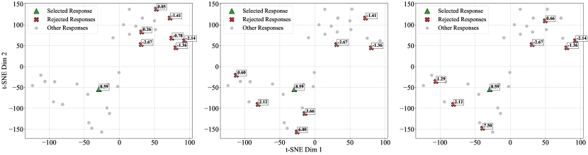
(a) 1.

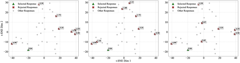
(b) 2.

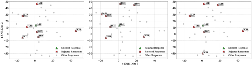
(c) 3.

Figure 5: t-SNE visualization of projected high-dimensional response embeddings into a 2D space, illustrating the separation of actively selected responses. (a) AMPO-BottomK (baseline). (b) AMPO-Coreset (ours). (c) Opt-Select (ours). Traditional baselines select many responses close to each other based on their rating, providing insufficient feedback to the LLM during preference optimization. In contrast, our methods optimize for objectives including coverage, generation probability, and preference rating.

References

- Arya et al. (2001) Arya, V., Garg, N., Khandekar, R., Meyerson, A., Munagala, K., and Pandit, V. Local search heuristic for k-median and facility location problems. In Proceedings of the thirty-third annual ACM symposium on Theory of computing, pp. 21–29, 2001.
- Askell et al. (2021) Askell, A., Bai, Y., Chen, A., Drain, D., Ganguli, D., Henighan, T., Jones, A., Joseph, N., Mann, B., DasSarma, N., et al. A general language assistant as a laboratory for alignment. arXiv preprint arXiv:2112.00861, 2021.
- Bachem et al. (2017) Bachem, O., Lucic, M., and Krause, A. Practical coreset constructions for machine learning. arXiv preprint arXiv:1703.06476, 2017.
- Bai et al. (2022) Bai, Y., Jones, A., Ndousse, K., Askell, A., Chen, A., DasSarma, N., Drain, D., Fort, S., Ganguli, D., Henighan, T., et al. Training a helpful and harmless assistant with reinforcement learning from human feedback. arXiv preprint arXiv:2204.05862, 2022.
- Cacchiani et al. (2022) Cacchiani, V., Iori, M., Locatelli, A., and Martello, S. Knapsack problems—an overview of recent advances. part ii: Multiple, multidimensional, and quadratic knapsack problems. Computers & Operations Research, 143:105693, 2022.
- Ceravolo et al. (2024) Ceravolo, P., Mohammadi, F., and Tamborini, M. A. Active learning methodology in llms fine-tuning. In 2024 IEEE International Conference on Cyber Security and Resilience (CSR), pp. 743–749. IEEE, 2024.
- Chen et al. (2024a) Chen, H., He, G., Yuan, L., Cui, G., Su, H., and Zhu, J. Noise contrastive alignment of language models with explicit rewards. arXiv preprint arXiv:2402.05369, 2024a.
- Chen et al. (2020) Chen, T., Kornblith, S., Swersky, K., Norouzi, M., and Hinton, G. E. Big self-supervised models are strong semi-supervised learners. Advances in neural information processing systems, 33:22243–22255, 2020.
- Chen et al. (2024b) Chen, Z., Deng, Y., Yuan, H., Ji, K., and Gu, Q. Self-play fine-tuning converts weak language models to strong language models. arXiv preprint arXiv:2401.01335, 2024b.
- Christiano et al. (2017) Christiano, P. F., Leike, J., Brown, T., Martic, M., Legg, S., and Amodei, D. Deep reinforcement learning from human preferences. Advances in neural information processing systems, 30, 2017.
- Cohen-Addad et al. (2021) Cohen-Addad, V., Saulpic, D., and Schwiegelshohn, C. A new coreset framework for clustering. In Proceedings of the 53rd Annual ACM SIGACT Symposium on Theory of Computing, pp. 169–182, 2021.
- Cohen-Addad et al. (2022) Cohen-Addad, V., Green Larsen, K., Saulpic, D., Schwiegelshohn, C., and Sheikh-Omar, O. A. Improved coresets for euclidean -means. Advances in Neural Information Processing Systems, 35:2679–2694, 2022.
- Cohn et al. (1996) Cohn, D. A., Ghahramani, Z., and Jordan, M. I. Active learning with statistical models. Journal of artificial intelligence research, 4:129–145, 1996.
- Cui et al. (2023) Cui, G., Yuan, L., Ding, N., Yao, G., Zhu, W., Ni, Y., Xie, G., Liu, Z., and Sun, M. Ultrafeedback: Boosting language models with high-quality feedback. arXiv preprint arXiv:2310.01377, 2023.
- Dong et al. (2023) Dong, H., Xiong, W., Goyal, D., Zhang, Y., Chow, W., Pan, R., Diao, S., Zhang, J., Shum, K., and Zhang, T. Raft: Reward ranked finetuning for generative foundation model alignment. arXiv preprint arXiv:2304.06767, 2023.
- Dubey et al. (2024) Dubey, A., Jauhri, A., Pandey, A., Kadian, A., Al-Dahle, A., Letman, A., Mathur, A., Schelten, A., Yang, A., Fan, A., et al. The llama 3 herd of models. arXiv preprint arXiv:2407.21783, 2024.
- Dubois et al. (2024) Dubois, Y., Galambosi, B., Liang, P., and Hashimoto, T. B. Length-controlled alpacaeval: A simple way to debias automatic evaluators. arXiv preprint arXiv:2404.04475, 2024.
- Ethayarajh et al. (2024) Ethayarajh, K., Xu, W., Muennighoff, N., Jurafsky, D., and Kiela, D. Kto: Model alignment as prospect theoretic optimization. arXiv preprint arXiv:2402.01306, 2024.
- Feldman (2020) Feldman, D. Core-sets: Updated survey. Sampling techniques for supervised or unsupervised tasks, pp. 23–44, 2020.
- Feldman et al. (2020) Feldman, D., Schmidt, M., and Sohler, C. Turning big data into tiny data: Constant-size coresets for k-means, pca, and projective clustering. SIAM Journal on Computing, 49(3):601–657, 2020.
- Gupta & Tangwongsan (2008) Gupta, A. and Tangwongsan, K. Simpler analyses of local search algorithms for facility location. arXiv preprint arXiv:0809.2554, 2008.
- Gupta et al. (2024a) Gupta, T., Madhavan, R., Zhang, X., Bansal, C., and Rajmohan, S. Refa: Reference free alignment for multi-preference optimization. arXiv preprint arXiv:2412.16378, 2024a.
- Gupta et al. (2024b) Gupta, T., Madhavan, R., Zhang, X., Bansal, C., and Rajmohan, S. Swepo: Simultaneous weighted preference optimization for group contrastive alignment, 2024b. URL https://arxiv.org/abs/2412.04628.
- Har-Peled & Mazumdar (2004) Har-Peled, S. and Mazumdar, S. On coresets for k-means and k-median clustering. In Proceedings of the thirty-sixth annual ACM symposium on Theory of computing, pp. 291–300, 2004.
- Hartigan & Wong (1979) Hartigan, J. A. and Wong, M. A. Algorithm as 136: A k-means clustering algorithm. Journal of the royal statistical society. series c (applied statistics), 28(1):100–108, 1979.
- Hong et al. (2024) Hong, J., Lee, N., and Thorne, J. Orpo: Monolithic preference optimization without reference model. In Proceedings of the 2024 Conference on Empirical Methods in Natural Language Processing, pp. 11170–11189, 2024.
- Huang et al. (2019) Huang, L., Jiang, S., and Vishnoi, N. Coresets for clustering with fairness constraints. Advances in neural information processing systems, 32, 2019.
- Kellerer et al. (2004a) Kellerer, H., Pferschy, U., Pisinger, D., Kellerer, H., Pferschy, U., and Pisinger, D. Introduction to np-completeness of knapsack problems. Knapsack problems, pp. 483–493, 2004a.
- Kellerer et al. (2004b) Kellerer, H., Pferschy, U., Pisinger, D., Kellerer, H., Pferschy, U., and Pisinger, D. Multidimensional knapsack problems. Springer, 2004b.
- Korbak et al. (2023) Korbak, T., Shi, K., Chen, A., Bhalerao, R. V., Buckley, C., Phang, J., Bowman, S. R., and Perez, E. Pretraining language models with human preferences. In International Conference on Machine Learning, pp. 17506–17533. PMLR, 2023.
- Kumar et al. (2024) Kumar, A., Zhuang, V., Agarwal, R., Su, Y., Co-Reyes, J. D., Singh, A., Baumli, K., Iqbal, S., Bishop, C., Roelofs, R., et al. Training language models to self-correct via reinforcement learning. arXiv preprint arXiv:2409.12917, 2024.
- Liu et al. (2024a) Liu, A., Bai, H., Lu, Z., Sun, Y., Kong, X., Wang, S., Shan, J., Jose, A. M., Liu, X., Wen, L., et al. Tis-dpo: Token-level importance sampling for direct preference optimization with estimated weights. arXiv preprint arXiv:2410.04350, 2024a.
- Liu et al. (2024b) Liu, C. Y., Zeng, L., Liu, J., Yan, R., He, J., Wang, C., Yan, S., Liu, Y., and Zhou, Y. Skywork-reward: Bag of tricks for reward modeling in llms. arXiv preprint arXiv:2410.18451, 2024b.
- Liu et al. (2024c) Liu, J., Zhou, Z., Liu, J., Bu, X., Yang, C., Zhong, H.-S., and Ouyang, W. Iterative length-regularized direct preference optimization: A case study on improving 7b language models to gpt-4 level. arXiv preprint arXiv:2406.11817, 2024c.
- Liu et al. (2021) Liu, X., Zhang, F., Hou, Z., Mian, L., Wang, Z., Zhang, J., and Tang, J. Self-supervised learning: Generative or contrastive. IEEE transactions on knowledge and data engineering, 35(1):857–876, 2021.
- Long et al. (2024) Long, D. X., Ngoc, H. N., Sim, T., Dao, H., Joty, S., Kawaguchi, K., Chen, N. F., and Kan, M.-Y. Llms are biased towards output formats! systematically evaluating and mitigating output format bias of llms. arXiv preprint arXiv:2408.08656, 2024.
- Meng et al. (2024) Meng, Y., Xia, M., and Chen, D. Simpo: Simple preference optimization with a reference-free reward. arXiv preprint arXiv:2405.14734, 2024.
- Oh Song et al. (2017) Oh Song, H., Jegelka, S., Rathod, V., and Murphy, K. Deep metric learning via facility location. In Proceedings of the IEEE Conference on Computer Vision and Pattern Recognition, pp. 5382–5390, 2017.
- Ouyang et al. (2022) Ouyang, L., Wu, J., Jiang, X., Almeida, D., Wainwright, C., Mishkin, P., Zhang, C., Agarwal, S., Slama, K., Ray, A., et al. Training language models to follow instructions with human feedback. Advances in neural information processing systems, 35:27730–27744, 2022.
- Pang et al. (2024) Pang, R. Y., Yuan, W., Cho, K., He, H., Sukhbaatar, S., and Weston, J. Iterative reasoning preference optimization. arXiv preprint arXiv:2404.19733, 2024.
- Park et al. (2024) Park, R., Rafailov, R., Ermon, S., and Finn, C. Disentangling length from quality in direct preference optimization. arXiv preprint arXiv:2403.19159, 2024.
- Qi et al. (2024) Qi, B., Li, P., Li, F., Gao, J., Zhang, K., and Zhou, B. Online dpo: Online direct preference optimization with fast-slow chasing. arXiv preprint arXiv:2406.05534, 2024.
- Rafailov et al. (2024) Rafailov, R., Sharma, A., Mitchell, E., Manning, C. D., Ermon, S., and Finn, C. Direct preference optimization: Your language model is secretly a reward model. Advances in Neural Information Processing Systems, 36, 2024.
- Sener & Savarese (2017) Sener, O. and Savarese, S. Active learning for convolutional neural networks: A core-set approach. arXiv preprint arXiv:1708.00489, 2017.
- Settles (2009) Settles, B. Active learning literature survey. 2009.
- Silver et al. (2016) Silver, D., Huang, A., Maddison, C. J., Guez, A., Sifre, L., Van Den Driessche, G., Schrittwieser, J., Antonoglou, I., Panneershelvam, V., Lanctot, M., et al. Mastering the game of go with deep neural networks and tree search. nature, 529(7587):484–489, 2016.
- Silver et al. (2017) Silver, D., Schrittwieser, J., Simonyan, K., Antonoglou, I., Huang, A., Guez, A., Hubert, T., Baker, L., Lai, M., Bolton, A., et al. Mastering the game of go without human knowledge. nature, 550(7676):354–359, 2017.
- Tran et al. (2023) Tran, H., Glaze, C., and Hancock, B. Iterative dpo alignment. Technical report, Technical report, Snorkel AI, 2023.
- Wu et al. (2024) Wu, Y., Sun, Z., Yuan, H., Ji, K., Yang, Y., and Gu, Q. Self-play preference optimization for language model alignment. arXiv preprint arXiv:2405.00675, 2024.
- Wu et al. (2023) Wu, Z., Hu, Y., Shi, W., Dziri, N., Suhr, A., Ammanabrolu, P., Smith, N. A., Ostendorf, M., and Hajishirzi, H. Fine-grained human feedback gives better rewards for language model training. Advances in Neural Information Processing Systems, 36:59008–59033, 2023.
- Xiao et al. (2023) Xiao, R., Dong, Y., Zhao, J., Wu, R., Lin, M., Chen, G., and Wang, H. Freeal: Towards human-free active learning in the era of large language models. arXiv preprint arXiv:2311.15614, 2023.
- Xu et al. (2024) Xu, H., Sharaf, A., Chen, Y., Tan, W., Shen, L., Durme, B. V., Murray, K., and Kim, Y. J. Contrastive preference optimization: Pushing the boundaries of LLM performance in machine translation. ArXiv, abs/2401.08417, 2024.
- Yu et al. (2024) Yu, Y., Zhuang, Y., Zhang, J., Meng, Y., Ratner, A. J., Krishna, R., Shen, J., and Zhang, C. Large language model as attributed training data generator: A tale of diversity and bias. Advances in Neural Information Processing Systems, 36, 2024.
- Yuan et al. (2024) Yuan, W., Kulikov, I., Yu, P., Cho, K., Sukhbaatar, S., Weston, J., and Xu, J. Following length constraints in instructions. arXiv preprint arXiv:2406.17744, 2024.
- Yuan et al. (2023) Yuan, Z., Yuan, H., Tan, C., Wang, W., Huang, S., and Huang, F. Rrhf: Rank responses to align language models with human feedback without tears. arXiv preprint arXiv:2304.05302, 2023.
- Zeng et al. (2024) Zeng, Y., Liu, G., Ma, W., Yang, N., Zhang, H., and Wang, J. Token-level direct preference optimization. arXiv preprint arXiv:2404.11999, 2024.
- Zhang et al. (2022) Zhang, Y., Feng, S., and Tan, C. Active example selection for in-context learning. arXiv preprint arXiv:2211.04486, 2022.
- Zheng et al. (2023) Zheng, L., Chiang, W.-L., Sheng, Y., Zhuang, S., Wu, Z., Zhuang, Y., Lin, Z., Li, Z., Li, D., Xing, E., et al. Judging llm-as-a-judge with mt-bench and chatbot arena. Advances in Neural Information Processing Systems, 36:46595–46623, 2023.