Beyond In-Distribution Success: Scaling Curves of CoT Granularity for Language Model Generalization

Abstract

Generalization to novel compound tasks under distribution shift is important for deploying transformer-based language models (LMs). This work investigates Chain-of-Thought (CoT) reasoning as a means to enhance OOD generalization. Through controlled experiments across several compound tasks, we reveal three key insights: (1) While QA-trained models achieve near-perfect in-distribution accuracy, their OOD performance degrades catastrophically, even with 10000k+ training examples; (2) the granularity of CoT data strongly correlates with generalization performance; finer-grained CoT data leads to better generalization; (3) CoT exhibits remarkable sample efficiency, matching QA performance with much less (even 80%) data.

Theoretically, we demonstrate that compound tasks inherently permit shortcuts in Q-A data that misalign with true reasoning principles, while CoT forces internalization of valid dependency structures, and thus can achieve better generalization. Further, we show that transformer positional embeddings can amplify generalization by emphasizing subtask condition recurrence in long CoT sequences. Our combined theoretical and empirical analysis provides compelling evidence for CoT reasoning as a crucial training paradigm for enabling LM generalization under real-world distributional shifts for compound tasks.

1 Introduction

Transformer-based language models (LMs) [4, 6, 45] have demonstrated unprecedented capabilities in knowledge retrieval [23, 49, 50] and reasoning [14, 8], driven by large-scale pretraining on diverse text corpora [37, 51, 30]. While these models excel at tasks with clear input-output mappings, their ability to generalize to compound tasks—those requiring dynamic planning, multi-step reasoning, and adaptation to evolving contexts—remains a critical challenge. Real-world applications such as GUI automation [48, 54, 42, 39, 47], textual puzzle solving [12, 41], and strategic gameplay like poker [13, 57, 18] demand not only procedural knowledge but also the capacity to handle distribution shift between training and deployment environments.

A central challenge lies in the misalignment between training data and deployment environments. For instance, consider a medical diagnosis system trained on historical patient records: it may falter when encountering novel symptom combinations during a disease outbreak or misalign with updated clinical guidelines (e.g., revised thresholds for ”high-risk” biomarkers [52]). Such distribution shifts can significantly degrade the performance of LMs trained on limited training datasets, underscoring the importance of generalization for reliable deployment.

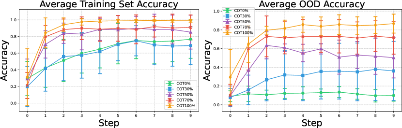
Figure 1: The illustration of the impact of the granularity of Chain-of-Thought on In-Distribution (IID) and Out-of-Distribution (OOD) performance. Left: IID performance. Right: OOD performance. Results are averaged over four compound tasks. While models trained without CoT achieve high IID accuracy ( 80%), they exhibit a substantially poor generalization performance ( 10%) on OOD data.

In this paper, we investigate how data collection impacts the generalization of LMs in compound tasks. Traditional approaches that prioritize direct instruction-result pairs (analogous to question-answering frameworks) optimize for task-specific accuracy but inadequately prepare models for compositional reasoning in unseen contexts. Recent advances in Chain-of-Thought (CoT) prompting [49], which elicit intermediate reasoning steps, suggest that explicit process supervision can enhance generalization. However, acquiring high-quality CoT annotations at scale remains prohibitively expensive [28, 22], raising a pivotal question: How do different data collection strategies, e.g., result-oriented Q-A pairs and CoT—affect the generalization of LMs to novel compound tasks?

To address this, we conduct controlled experiments using synthetic compound tasks that systematically introduce distribution shifts between training and evaluation environments. We evaluate LMs trained on two data paradigms: (1) result-oriented Q-A pairs and (2) CoT sequences of varying granularity. Our analysis reveals three critical insights: (i) Generalization Gap: While both Q-A and CoT-trained LMs achieve near-perfect in-distribution accuracy, Q-A models exhibit severe performance degradation under distribution shifts—even with 10000k training examples. (ii) Granularity-Generalization Tradeoff: The granularity of CoT data strongly correlates with generalization performance; finer-grained CoT data leads to better generalization. (iii) Sample Efficiency: LMs trained with fine-grained CoT data demonstrate strong sample efficiency, achieving comparable generalization to Q-A pair training with substantially less data. These results suggest that even small amounts of high-quality CoT data can significantly enhance LM generalization, despite the challenges associated with its collection.

Inspired by the recent work [29], we further theoretically demonstrate that compound tasks inherently contain shortcuts—superficial patterns in Q-A data that enable high in-distribution accuracy but misalign with underlying reasoning principles. CoT training mitigates this by decomposing tasks into structured subtasks, forcing models to internalize valid reasoning paths. Leveraging transformer positional embeddings, we further show that explicitly emphasizing subtask conditions within CoT sequences further reduces shortcut reliance, especially in the long CoT setting.

In summary, our paper makes the following key contributions: (1) We establish a controlled experimental framework to quantify the impact of data collection strategies on LM generalization under distribution shifts. Based on it, we demonstrate that LMs trained directly on question-answer pairs can achieve high accuracy on in-distribution data for new tasks but exhibit poor generalization, even when trained on substantial datasets (e.g., 10000k examples). (2) Through systematic scaling experiments, we demonstrate that fine-grained CoT data enhances generalization and sample efficiency, even with limited training data. (3) We provide theoretical insights into how CoT helps to mitigate shortcut learning, thus improving generalization and further demonstrate that, with longer CoT chains, repeating the sub-task condition can further improve LMs generalization capability. We believe our findings provide a reliable guide for data collection practices when leveraging LMs for novel tasks.

2 Related Work

Generalization in LLMs

Transformer-based language models [46] demonstrate strong performance on in-distribution tasks [33, 34, 53] but often struggle with OOD tasks due to challenges such as distribution shifts [2, 56], shortcut learning [29, 11], and overfitting [26], where the correlations they exploit no longer hold [38, 36].

Various approaches have been proposed to mitigate shortcut learning, including data augmentation [15, 58] and adversarial training [19, 43], though many methods remain task-specific and lack generalization. Prior work [5] evaluates OOD performance by comparing models across datasets, but without precise control over distribution shifts. Our work introduces a fully controlled experimental setup, explicitly defining and manipulating shifts to better analyze model adaptation.

Chain-of-Thought Reasoning

CoT reasoning enables multi-step derivations, allowing models to articulate reasoning [49, 23, 59, 10, 21], while its underlying mechanism remains unclear. Recent theoretical works apply circuit complexity theory to analyze CoT’s fundamental capabilities [27, 1, 9], while other studies examine how CoT structures intermediate steps to decompose complex tasks [44, 24, 55, 3].

CoT has been shown to improve performance on tasks with shared reasoning patterns, even under distribution shifts [25, 17]. In zero-shot and few-shot settings, it leverages step-by-step exemplars to apply pre-trained knowledge beyond training data [22]. Recent studies emphasize fine-grained CoT, where detailed intermediate steps enhance task learning and reduce shortcut reliance [35, 7].

Scaling Laws

Scaling laws define the relationship between model size, data scale, and performance in LLMs [20, 16, 6]. However, scaling alone is insufficient under significant distribution shifts, as larger models may amplify shortcut learning or overfit to surface patterns [32]. Optimizing the ratio of CoT reasoning in training data and validating its real-world effectiveness remain open challenges. Structured intermediate representations further aid in overcoming global obstacles and improving generalization [1]. Our findings indicate that incorporating CoT reasoning into the training process enhances the robustness of LLMs when addressing distribution shifts, particularly in out-of-distribution tasks.

Figure 2: The illustration of shortcut learning, wherein the model exploits spurious correlations between questions and answers (e.g., answer length) rather than genuinely understanding the underlying reasoning, ultimately results in poor generalization ability.

3 Preliminary

This paper investigates the generalization capabilities of transformer-based language models when applied to compound tasks characterized by dynamic dependencies among sub-tasks. Unlike standard sequential processing, compound tasks involve inter-related actions where the state of each action depends on a varying subset of previous actions. These dependencies are not static but evolve based on the task’s progress, posing a unique challenge for models trained on sequential text. For example, consider preparing a complex meal with multiple dishes. The cooking state of pasta, for instance, depends on whether the sauce is freshly made or pre-made, demonstrating how dynamic dependencies can arise. This scenario reflects the intricate structure of many real-world tasks where a simple sequential reading fails to capture the underlying relationships between actions.

We formalize compound tasks through a state transition framework with dynamic dependencies, motivated by real-world scenarios like software development: subtask states (e.g., database setup, API integration) evolve through context-dependent interactions.

3.1 Compound Task Structure

A compound task organizes complex operations through a hierarchical tree of subtasks. The structure comprises atomic actions at leaf nodes and interconnected subtasks at higher levels, with dynamic dependencies governing their execution flow. As illustrated in 3, the system processes these tasks sequentially, evaluating dependencies and aggregating results from completed subtasks to achieve the overall objective. This flexible architecture allows for modification and reorganization of subtasks to accommodate evolving requirements.

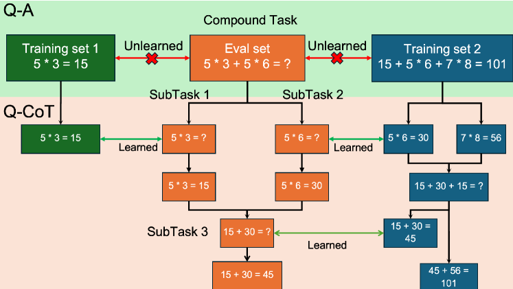
Figure 3: Chain-of-thought alleviates distribution shift by breaking down complex problems into simpler, familiar sub-problems.

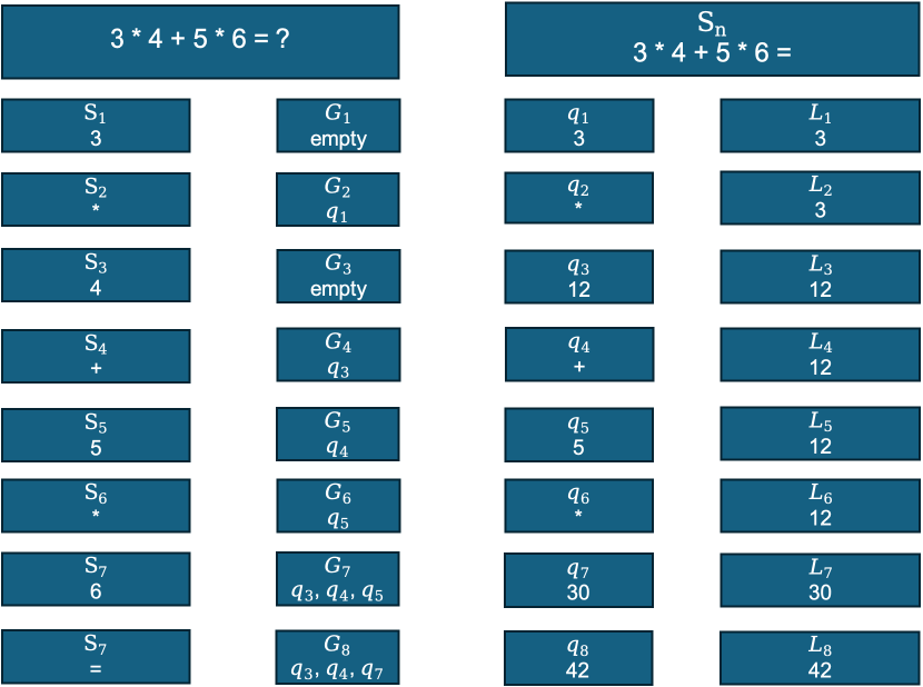
Figure 9: Step by Step explanation on definition 3.1

To accommodate transformer models’ input format requirements, we define the compound task at the token level. Figure 9 provides a step-by-step illustration demonstrating how this definition integrates into the task structure.

Definition 3.1.

Given the input sequence $S=(s_{1},\ldots,s_{n})$ and subtask state sequence $Q=(q_{1},\ldots,q_{n})$ where $Q^{i}=(q_{1},\ldots,q_{i})$ denotes the prefix subsequence contains the first $i$ states of $Q$, CP($n$) is defined:

Dynamic Graph Evolution: At step $i+1$, the dependency graph updates with a function $B:S^{i+1}\times\mathbb{N}\to\mathcal{P}(\mathbb{N})$:

$$G_{i+1}=G(q_{1},\ldots,q_{i}\mid s_{1},\ldots,s_{i+1})$$

$$=\{q_{k}\mid k\in B(s_{1},\ldots,s_{i+1},i+1)\}$$ (1)

where $B(s_{1},\ldots,s_{i},j)$ returns the set of indices that determine the dynamic dependencies based on the current state sequence and global semantic constraints.

State Transition Function $F:\mathcal{P}(Q^{i})\times Q^{i}\to q$ computes the next state using selected predecessors from the prefix subsequence $Q^{i}$:

$$\begin{split}q_{i+1}&=F(G(q_{1},\ldots,q_{i}\mid s_{1},\ldots,s_{i+1}),s_{i+1})\\ &\text{where}\quad F(\emptyset)=\text{Constant}\end{split}$$

Final Result Operation: The system’s final result is computed through a sequence of operations $L_{i}$ that aggregate states progressively: $L:q\times q\rightarrow R$

$$\begin{split}L_{1}&=H(\emptyset,q_{1})=q_{1}\\ L_{i}&=H(L_{i-1},q_{i})\quad\text{for }i=2,\ldots,N\end{split}$$

where $H$ is an aggregation function like maximum, minimum, or summation function and $H(\emptyset,q)=q$ that can be specialized as needed.

Problem Setting

To investigate the generalization capabilities of transformer-based language models, we establish a comprehensive training and evaluation framework across different complexity levels. Our framework involves training the model on problems of complexity levels $n_{1}$ and $n_{2}$, while evaluating on problems of complexity $n_{3}$, where $n_{3}$ is strategically chosen between $n_{1}$ and $n_{2}$. Formally, let $X^{n}=(s_{1},s_{2},...,s_{n})$ denote the input question text for CP($n$) problems and $Y^{n}=(y_{1},y_{2},...,y_{n})$ represent their corresponding output answers. The transformer model is trained on the mappings $X^{n_{1}}\rightarrow Y^{n_{1}}$ and $X^{n_{2}}\rightarrow Y^{n_{2}}$, and subsequently evaluated on $X^{n_{3}}\rightarrow Y^{n_{3}}$, where $n_{1}\neq n_{2}\neq n_{3}$. The strategic selection of $n_{3}$ within the interval $(n_{1},n_{2})$ is informed by the token distribution patterns observed in transformer training. Since CP($n_{2}$) problems typically encompass the token vocabulary required for CP($n_{3}$), this ensures that the model’s token embeddings are adequately trained for the evaluation tasks. This approach helps minimize the impact of unseen tokens during OOD evaluation, enabling us to focus on assessing the transformer’s fundamental reasoning capabilities rather than its ability to handle novel vocabulary. In our experiments, we utilize two types of training data:

• Question-Answer pairs (Q-A): Constructed using $X^{n}$ as input and $Y^{n}$ containing only the final answer token (e.g., the length of the longest increasing sequence)

• Question-CoT pairs (Q-CoT): Constructed using $X^{n}$ as input and $Y^{n}$ containing the complete Chain of Thought tokens as defined in Section 4.1

4 Theoretical Analysis

In order to explain how CoT training mitigates shortcut learning and distribution shifts in compound tasks. We perform theoretical analysis in three stages: (1) characterizing transformer shortcut learning mechanisms, (2) deriving structural conditions for effective CoT sequences, and (3) quantifying CoT’s generalization benefits through distribution shift theory. We will present details as follows:

4.1 Shortcuts via Transformer

Shortcut learning [11, 40], wherein models exploit spurious correlations instead of learning robust, generalizable features, poses a significant challenge to OOD generalization. In the context of compound tasks, transformers, despite their capacity for complex computations, can be susceptible to learning trivial shortcuts, particularly when training data exhibits systematic patterns. We can easily construct a trivial shortcut example in the compound task setting.
For a compound task with two patterns having different token lengths $n_{1}$, $n_{2}$, transformers can learn shortcuts for classification and memorization. Let $T:n\to{0,1}$ be the binary classifier that identifies pattern type based on sequence length. The shortcut solution consists of two steps:

1. Pattern Classification: Using $O(1)$ attention heads to distinguish sequence lengths by uniform attention over all positions.

2. Pattern Memorization: After identifying the pattern type, the transformer uses $O(\max(n_{1},n_{2}))$ layers with attention heads to capture position-dependent features of the input sequence.

The total complexity is $O(\max(n_{1},n_{2}))$ layers, with each layer requiring attention heads to learn position-specific patterns. This provides a more efficient solution compared to memorizing all possible question-answer pairs in the training set, as it leverages the structural property of sequence length for classification.

4.2 Recap Conditions for Effective Chain of Thought

Figure 4: Outside Window Recap Condition: Recapping a token from outside the attention window, s5 depends on s1

Figure 5: Inside Window Recap Condition: Recapping tokens to preserve causal order and skip the irrelevant token, s6 depends on s1 and s3

Before introducing the Chain of Thought [49] approach, we establish two fundamental conditions that enable more effective reasoning chains:
1. Outside Window Recap Condition Due to finite precision constraints, only tokens with the top-k attention scores can be effectively recalled. When the distance between the target token position and current position exceeds a threshold, the attention scores become negligible within the given precision, preventing recall of tokens outside this window. This necessitates strategic recapping of tokens within the window to maintain information flow. See C.1 for formal analysis.
2. Inside Window Recap Condition: For optimal model performance, tokens within the attention window should be organized following the ground truth causal order, avoiding irrelevant intermediary tokens that could impede convergence. As proven in C.2, including irrelevant tokens in the sequence slows down model convergence. Therefore, we must carefully structure the token sequence within the window (e.g., through techniques like reverse ordering or selective token repetition) to align with the underlying causal structure.
Combined with these two recap conditions, for each inference step in a compound task, we must ensure all dependent tokens are both compactly positioned and arranged in their causal order. This strategy enables effective information flow while maintaining computational efficiency. In implementation, since tokens may have multiple dependencies, it is preferable to copy tokens rather than move them.

4.3 Chain of Thought Suppresses the Shortcuts

Inspired by recent work [27, 9] and building upon our recap conditions, we now introduce a CoT formalization specifically designed to capture the dynamic state transitions in compound tasks. Rather than allowing the model to learn superficial shortcuts, our CoT format explicitly tracks the evolving dependencies and state transitions that characterize the ground truth recurrent solution.

Definition 4.1 (Chain of Thought).

Input: $$\;s_{1}\mid\cdots\mid s_{N}$$

CoT Steps: $$\;\langle\text{sep}\rangle\;s_{2}\mid G_{2}\mid q_{2}\mid L_{1}\mid L_{2}$$

$$\;\langle\text{sep}\rangle\;\cdots$$

$$\;\langle\text{sep}\rangle\;s_{N}\mid G_{N}\mid q_{N}\mid L_{N-1}\mid L_{N}$$

This format structures each step to track dependencies ($G_{i}$), states ($q_{i}$), and intermediate results ($L_{i}$), guiding the model toward learning true solution dynamics. Remarkably, this principled approach can be implemented with minimal architectural requirements:

Proposition 4.2.

For any compound problem satisfying Definition 3.1, and for any input length bound $n\in\mathbb{N}$, there exists an autoregressive Transformer with:

• Constant depth $L$

• Constant hidden dimension $d$

• Constant number of attention heads $H$

where $L$, $d$, and $H$ are independent of $n$, such that the Transformer correctly generates the Chain-of-Thought solution defined in Definition 4.1 for all input sequences of length at most $n$. Furthermore, all parameter values in the Transformer are bounded by $O(\text{poly}(n))$.

4.4 Distribution Shift Analysis for Q-A vs. Q-CoT

Understanding the distribution shift between traditional Q-A and CoT approaches is crucial for analyzing OOD generalization. This section examines how CoT’s intermediate reasoning steps influence the alignment between training and evaluation distributions. We analyze a dynamic state-transition system where problems of different lengths are processed through either direct Q-A or through CoT reasoning 3. Specifically, we compare: 1. Q-A training/evaluation on problem lengths $\{n_{1},n_{2}\}$ (train) and $n_{3}$ (eval). 2. Q-CoT training/evaluation on problem lengths $\{n_{1},n_{2}\}$ (train) and $n_{3}$ (eval). We assume $n_{1}<n_{3}<n_{2}$, and let

$$\mathcal{D}_{\text{train}}^{\text{Q-A}}\;=\;\Bigl{\{}(X^{n_{1}},Y^{n_{1}}),\,(X^{n_{2}},Y^{n_{2}})\Bigr{\}},\quad$$

$$\mathcal{D}_{\text{eval}}^{\text{Q-A}}\;=\;\Bigl{\{}(X^{n_{3}},Y^{n_{3}})\Bigr{\}},$$

be the respective datasets in the Q-A setup. Analogously, in the Q-CoT setup, each problem instance is expanded into subproblem–subsolution pairs (the chain-of-thought states). Denote:

$$\mathcal{D}_{\text{train}}^{\text{Q-CoT}}\;=\;\Bigl{\{}\bigl{(}X^{n_{1}},\{q_{i}^{(n_{1})}\},Y^{n_{1}}\bigr{)},\,\bigl{(}X^{n_{2}},\{q_{i}^{(n_{2})}\},Y^{n_{2}}\bigr{)}\Bigr{\}},\quad$$

$$\mathcal{D}_{\text{eval}}^{\text{Q-CoT}}\;=\;\Bigl{\{}\bigl{(}X^{n_{3}},\{q_{i}^{(n_{3})}\},Y^{n_{3}}\bigr{)}\Bigr{\}}.$$

Here $\{q_{i}^{(n)}\}$ denotes the chain-of-thought states or subsolutions for a length-$n$ problem.

We let $P_{\text{train}}^{\text{Q-A}}$, $P_{\text{eval}}^{\text{Q-A}}$, $P_{\text{train}}^{\text{Q-CoT}}$, and $P_{\text{eval}}^{\text{Q-CoT}}$ be the corresponding data or model-induced distributions over Q-A setting or Q-CoT setting.

Our analysis begins with a fundamental result about the structure of CoT sequences in our dynamic system.

4.4.1 Prefix-Substructure Theorem in a Dynamic State-Transition System

A key property of chain-of-thought sequences is that prefix relationships between input sequences carry over to their states, enabling shorter problems CP($n_{3}$) to embed within longer ones CP($n_{2}$).

Lemma 4.3 (Prefix Substructure).

Let $S^{short}=(s_{1},s_{2},\ldots,s_{n_{2}})$ and let $S^{long}=(s_{1},s_{2},\ldots,s_{n_{3}})$ be its prefix, with $n_{3}<n_{2}$. Suppose their chain-of-thought sequences under the same $(G,F)$ are

$$Q^{short}\;=\;\bigl{(}q_{1}^{short},q_{2}^{short},\ldots,q_{n_{2}}^{short}\bigr{)}\quad\text{and}$$

$$\quad Q^{long}\;=\;\bigl{(}q_{1}^{long},q_{2}^{long},\ldots,q_{n_{3}}^{long}\bigr{)}.$$

Then for all $1\leq i\leq n_{3}$, we have

$$q_{i}^{long}\;=\;q_{i}^{short}.$$

Hence $\bigl{(}q_{1}^{long},\ldots,q_{n_{3}}^{long}\bigr{)}$ is exactly the prefix of $\bigl{(}q_{1}^{short},\ldots,q_{n_{2}}^{short}\bigr{)}$.

This property suggests CoT’s intermediate steps provide natural bridges between problems of different lengths, potentially easing distribution shift concerns.

4.4.2 Training Size Effects on Distribution Shift Through Prefix Coverage

Building upon the prefix-substructure property, we now quantify the distribution shift between training and evaluation sets for both Q-A and Q-CoT approaches. This analysis reveals how CoT’s intermediate reasoning steps can potentially mitigate distribution shift effects.

Theorem 4.4 (KL Divergence Reduction with Training Size).

Let $m_{1}$ and $m_{2}$ be the number of training sequences of length $n_{1}$ and $n_{2}$ respectively, with total training size $M=m_{1}+m_{2}$. Let $n_{1}<n_{3}<n_{2}$ where $n_{3}$ is the evaluation length and $m_{3}$ is the number of sequences in evaluation set. Then: 1. The coverage probability $P_{\text{cover}}(M)$ for prefixes of length $n_{3}$ is:

$$P_{\text{cover}}(M)=\frac{m_{2}}{m_{3}k^{n_{3}}}$$

where $k$ is the size of the input vocabulary $m_{2}\leq m_{3}k^{n_{3}}$.

2. The KL divergence between evaluation and training distributions under Q-CoT satisfies:

$$D_{\mathrm{KL}}\!\Bigl{(}P_{\text{eval}}^{\text{Q-CoT}}\,\big{\|}\,P_{\text{train}}^{\text{Q-CoT}}\Bigr{)}\;\leq\;(1-P_{\text{cover}}(M))\cdot D_{\mathrm{KL}}\!\Bigl{(}P_{\text{eval}}^{\text{Q-A}}\,\big{\|}\,P_{\text{train}}^{\text{Q-A}}\Bigr{)}$$

3. When $m_{2}=m_{3}k^{n_{3}}$:

$$D_{\mathrm{KL}}\!\Bigl{(}P_{\text{eval}}^{\text{Q-CoT}}\,\big{\|}\,P_{\text{train}}^{\text{Q-CoT}}\Bigr{)}=0$$

Remark 4.5 (Relationship with Training Size).

The relationship between distribution shift and training size $M$ is characterized by several interconnected aspects:

First, $P_{\text{cover}}(M)$ exhibits monotonic growth with training size $M$, reflecting increased coverage of prefix patterns in the training data. This directly influences the distribution shift reduction.

Second, the term $D_{\mathrm{KL}}\!\Bigl{(}P_{\text{eval}}^{\text{Q-A}}\,\big{\|}\,P_{\text{train}}^{\text{Q-A}}\Bigr{)}$ represents a fundamental structural difference between Q-A and Q-CoT approaches. This term remains constant regardless of training size $M$ and equals the Q-A distribution shift by construction.

The theorem implies that Q-CoT’s out-of-distribution (OOD) performance improves primarily through enhanced prefix coverage as training size increases. However, in practical scenarios, missing intermediate steps in the training data’s chain-of-thought sequences can significantly impact performance:

• Incomplete chains reduce $P_{\text{cover}}(M)$ due to corrupted prefix structures

• This reduction leads to a higher upper bound on the KL divergence $D_{\mathrm{KL}}\Bigl{(}P_{\text{eval}}^{\text{Q-CoT}}\,\big{\|}\,P_{\text{train}}^{\text{Q-CoT}}\Bigr{)}$

• Consequently, OOD performance with incomplete chains underperforms relative to complete Q-CoT settings

This analysis demonstrates that Chain-of-Thought’s intermediate reasoning steps effectively mitigate distribution shift between training and evaluation sets through improved prefix coverage, leading to enhanced out-of-distribution performance compared to traditional Q-A approaches.

5 Experiment

In order to investigate how data collection methods impact LMs’ generalization ability, we conducted controlled studies on three compound reasoning tasks with systematic distribution shifts. Our experiments address three key questions: (1) How does direct QA training compare to CoT in OOD generalization? (2) Can increasing data help direct QA training to generalize to OOD data? (3) Can repeat the conditions for each subtask of one compound task help generalization?

5.1 Setting

5.1.1 Task and Experiment setting

We evaluate the generalization ability of LMs through three compound reasoning tasks: (1) Longest Increasing Subsequence, (2) Multi-Step Path Counting, and (3) Equation Restoration with Variable Calculation.

• Longest Increasing Subsequence (LIS): Given an input sequence $X^{n}$ of integers, compute the length of the longest increasing subsequence. The model is trained on sequences of complexity levels $n_{1}=4$ and $n_{2}=16$, and evaluated on sequences of complexity $n_{3}=10$, examining the model’s ability to generalize across different sequence lengths and positional dependencies.

• Multi-Step Path Counting (MPC): Given an input sequence $X^{n}$ specifying the available steps (where 0 indicates a forbidden step, 1 means an available step), compute the number of unique paths to reach position n using steps of size {1,2,3}. The model is trained on problems of complexity levels $n_{1}=20$ and $n_{2}=40$, and evaluated on problems of complexity $n_{3}=30$, testing the model’s ability to generalize across different path constraints and combinatorial patterns.

• Equation Restoration and Variable Computation (ERVC): Given a dataset of observations containing $n$ variables and their values, recover $m$ underlying linear system of equations, and then use these recovered relationships to compute target variables under new value assignments. The model trains on systems of ERVC21-41($n_{1}=2$, $m_{1}=1$), ($n_{2}=4$, $m_{2}=1$) variables and equations for the first setting, and ERVC21-43($n_{1}=2$, $m_{1}=1$) and ($n_{2}=4$, $m_{2}=3$) for the second setting, while testing on ($n_{3}=3$, $m_{3}=1$) and ($n_{3}=3$, $m_{3}=2$) respectively, where distribution shifts arise from varying numbers of variables (n) and equations (m) in the system.

5.1.2 Training Datasets Preparation

For each task, we generated datasets follow the two formats:

• Question-Answer (Q-A): Datasets consist of input questions paired directly with the final answer, representing direct supervision without explicit reasoning steps. This corresponds to a CoT dropout rate of 0% (CoT-0%).

• Question-Chain-of-Thought (Q-CoT): Datasets include input questions paired with step-by-step Chain-of-Thought explanations leading to the final answer, providing process supervision. This represents a CoT dropout rate of 100% (CoT-100%).

To investigate the impact of partial CoT supervision, we also conducted ablation studies using probabilistic CoT dropout. In these settings, each step within a complete CoT demonstration has a probability of being retained in the training data. We explored dropout rates of 30%, 50%, and 70% (CoT-30%, CoT-50%, CoT-70%). We focus on probabilistic dropout as preliminary experiments with fixed-portion CoT dropout showed significant OOD performance degradation.

For scaling experiments, we varied the dataset size from 1k to 30k samples for both Q-A and Q-CoT regimes. Models were trained on the ID data splits and evaluated on both ID and OOD splits to measure generalization gaps.

5.1.3 Model Training and Evaluation

For the Longest Increasing Subsequence and Multi-Step Path Counting tasks, we implemented a 6-layer transformer architecture trained from scratch, featuring an embedding size of 256/512 and 16 attention heads. The Equation Restoration tasks were approached differently, utilizing the Phi-3.5-mini-instruct model as the foundation for task-specific fine-tuning. All model variants incorporate Rotary Position Embedding. In evaluating model performance, we employed different strategies for Q-A and Q-CoT data. For Q-A data in both the Longest Increasing Subsequence and Multi-Step Path Counting tasks, correctness is determined by comparing the token immediately preceding the <eos> token. For Q-CoT data, our evaluation extends beyond the final answer, incorporating intermediate computational tokens (such as $Q$ and $L$) that contribute to the solution. This comprehensive evaluation approach helps mitigate cases where incorrect reasoning processes might accidentally yield correct final answers through guessing.

5.2 Results Analysis

Table 1: Performance comparison across MPC, LIS, ERVC tasks, where ID denotes the in-distribution task, OOD denotes out-of-distribution task, ID-OOD denotes the different between ID and OOD performance.

Task	MPC		LIS		ERVC21-43		ERVC21-41
	Q-A	Q-CoT	Q-A	Q-CoT	Q-A	Q-CoT	Q-A	Q-CoT
ID $\uparrow$	0.83	1.0	0.97	0.995	0.39	1.0	0.49	0.95
OOD $\uparrow$	0.21	0.81	0.14	0.75	0.02	0.959	0.126	0.905
ID-OOD $\downarrow$	0.62	0.19	0.83	0.245	0.37	0.041	0.364	0.045

5.2.1 Generalization Gap and Scaling Curves

Figure LABEL:fig:scaling_results and Table 1 presents the accuracy scaling curves for MPC and LIS tasks as a function of dataset size, comparing different CoT ratios (0%, 30%, 50%, 70%, and 100%). Consistent with the theoretical predictions derived from Theorem 4.4 (referenced in the main paper), models trained with higher CoT percentages (CoT-70%, CoT-100%) exhibit significantly improved OOD generalization compared to direct QA models (CoT-0%). This is manifested in both faster initial performance gains and higher sustained accuracy levels as dataset size increases.

Specifically, for Q-A (CoT-0%), OOD performance plateaus rapidly with increasing data, indicating limited generalization. In contrast, Q-CoT models demonstrate continued OOD performance improvement with larger datasets, effectively mitigating the generalization gap. The observed performance gap between Q-CoT and Q-A is qualitatively consistent with the upper bound on KL divergence predicted by Theorem 4.4, which suggests that CoT supervision reduces distribution shift by enhancing prefix coverage.

Furthermore, the degraded OOD performance observed in partial CoT settings (CoT-30%, CoT-50%) empirically supports the theoretical argument that incomplete reasoning chains diminish prefix coverage, leading to increased KL divergence and reduced generalization.

These empirical findings strongly validate the theoretical framework, demonstrating that CoT supervision enhances OOD generalization by encoding explicit reasoning steps. This structured reasoning process appears to transform novel OOD problems into more familiar, in-distribution-like problems, enabling better generalization.

5.2.2 Granularity-Generalization Tradeoff

Figure LABEL:fig:combined demonstrates a clear relationship between CoT step coverage and OOD generalization performance across tasks. Specifically, models trained with more complete CoT steps exhibit superior generalization capabilities on OOD samples. To formally characterize this empirical observation, we develop a theoretical framework in with a simple linear model that quantitatively explains how the omission of CoT steps during training systematically degrades model performance. Our analysis reveals that the degradation follows an exponential decay pattern with respect to the number of missing steps, highlighting the critical importance of maintaining granular reasoning steps for robust generalization.

5.2.3 Data Scaling Experiments

To investigate the effect of training data scaling on generalization, we examined the performance trends as dataset size increased. As depicted in Figure LABEL:fig:scaling_results, a key observation emerges: models trained without CoT supervision exhibit limited improvement in OOD generalization despite substantial increases in training data size (up to 10,000k samples). While ID accuracy improves with larger datasets for these models, their OOD performance plateaus, indicating that even the increased data cannot help generalization to novel compound tasks with direct Q-A training. In stark contrast, models trained with CoT supervision demonstrate a distinct capacity to translate larger datasets into improved OOD generalization.

5.2.4 Sample Efficiency

As shown in Figure LABEL:fig:scaling_results, models trained with a higher percentage of CoT examples demonstrate superior sample efficiency in both MPC and LIS scaling experiments. Specifically, models with $70\%$ and $100\%$ CoT (CoT-$70\%$ and CoT-$100\%$) achieve a higher OOD accuracy with significantly smaller dataset sizes compared to models trained with lower CoT percentages. This effect is particularly pronounced in the small data regime (1k-10k samples), where CoT-$100\%$ maintains a relatively robust OOD performance ( 0.55-0.75 accuracy) while models with less CoT supervision struggle (below 0.4 accuracy). This suggests that incorporating more reasoning steps through CoT not only improves overall performance but also enables more efficient learning from limited training data.

5.2.5 Recap Condition Ablation

We investigate the impact of the recap condition on model performance in Equation Restoration tasks in Table 2. For ERVC21-43, models trained with the recap condition achieve a high training accuracy of 0.974 and maintain this level of performance on the OOD set (0.974). In contrast, models trained without the recap condition exhibit significantly lower accuracy on both the training set (0.436) and the OOD set (0.126). A similar trend is observed for ERVC21-41. The model with the recap condition achieves near-perfect training accuracy (0.997) and strong OOD performance (0.952). Conversely, the model without the recap condition shows substantially reduced accuracy in both training (0.638) and OOD settings (0.558). These results strongly suggest that the recap condition of each subtask plays a critical role in the generalization of LMs and and validate our theoretical propositions outlined in Section 4.2

Table 2: Model performance comparisons on the with and without recap condition on the Equation Restoration Task, where

Task	ERVC21-43		ERVC21-41
Dataset	Training	OOD	Training	OOD
w/ recap condition	0.974	0.947	0.997	0.952
w/o recap condition	0.436	0.126	0.638	0.558

6 Conclusion

In this paper, through controllable systematic experimentation and theoretical analysis in compound tasks, we demonstrate that (1) Direct QA-trained models exhibit dramatic performance degradation under shifts despite high in-distribution accuracy with even 100k data in the single task, (2) CoT granularity directly governs generalization strength, with fine-grained reasoning steps enabling higher OOD accuracy, and (3) CoT training achieves comparable performance to QA paradigms with much less data, underscoring its sample efficiency. Theoretically, we prove that compound tasks inherently permit spurious correlations in QA data, while CoT enforces structured reasoning paths, a process amplified by transformer positional embeddings through subtask condition recurrence. These findings provide a reliable guide for data collection practices when leveraging LMs for novel tasks. We will explore automated CoT generation and dynamic granularity adaptation to further reduce annotation costs in the future work.

Impact Statement

This paper offers a novel perspective, demonstrating the indispensable role of CoT in enhancing the generalization capabilities of LMs. Through theoretical analysis and comprehensive empirical experimentation, we establish CoT as a critical enabler of robust out-of-distribution generalization. Crucially, this work provides valuable guidance for the development of effective data curation strategies, specifically for collecting data that maximizes the benefits of CoT training. This guidance is directly applicable to the industrial deployment of LMs and the fine-tuning of large models for novel tasks, offering a pathway to improve the generalization and real-world utility of these models through informed data acquisition methodologies.

Appendix A Explain Compound task in formal definition

As shown in the figure, original tree like data structure can be converted to an array which is easily feeded into language model.

Appendix B Code and Data

We provide an anonymous page, you can following the instruction to generate data, training model and evaluation. https://github.com/physicsru/Scaling-Curves-of-CoT-Granularity-for-Language-Model-Generalization

Appendix C Recap Condition Analysis

Theorem C.1 (Outside Token Recap Condition under RoPE).

Consider a transformer with Rotary Positional Embedding (RoPE) using angles $\theta_{j}=10000^{-2j/d_{\text{model}}}$. Given finite computational precision $s$ and minimum resolvable attention score $\epsilon$, there exists a threshold distance $\tau>0$ such that for all positional distances $d>\tau$:

$$|A(d)|<\epsilon,$$

where $A(d)$ is the attention score between tokens at distance $d$. Consequently, tokens beyond $[i_{\text{current}}-\tau,i_{\text{current}}+\tau]$ cannot be recalled.

Proof.

Step 1: Attention Score Formulation The RoPE attention score between positions $m$ and $n$ (distance $d=|m-n|$) is:

$$A(d)=\text{Re}\left[\sum_{j=0}^{d_{\text{model}}/2-1}h_{j}e^{\mathbf{i}d\theta_{j}}\right],\quad h_{j}:=q_{[2j:2j+1]}\mathbf{k}^{*}_{[2j:2j+1]}$$

where $h_{j}$ encodes query-key interactions for the $j$-th dimension pair.

Step 2: Abel Transformation[31] Let $S_{j+1}=\sum_{k=0}^{j}e^{\mathbf{i}d\theta_{k}}$ with $S_{0}=0$. Using summation by parts:

$$\sum_{j=0}^{d_{\text{model}}/2-1}h_{j}e^{\mathbf{i}d\theta_{j}}=\sum_{j=0}^{d_{\text{model}}/2-1}(h_{j}-h_{j+1})S_{j+1}$$

Taking absolute values:

$$|A(d)|\leq\sum_{j=0}^{d_{\text{model}}/2-1}|h_{j+1}-h_{j}|\cdot|S_{j+1}|$$

Step 3: Bounding Query-Key Differences. Assume that the query and key representations are uniformly bounded so that $\|q\|,\,\|k\|\leq C$. In particular, since each $h_{j}$ results from a dot product between sub-vectors from $q$ and $k$, we have $|h_{j}|\leq C^{2}$. Moreover, if we assume that the embeddings vary smoothly with the index $j$ (as expected from the continuity of underlying network nonlinearities and weight matrices), then the mean value theorem implies that the difference

$$|h_{j+1}-h_{j}|$$

is bounded by a Lipschitz constant. That is, there exists a constant $M=\mathcal{O}(C^{2})$ such that for every $j$

$$|h_{j+1}-h_{j}|\leq M.$$

A more refined analysis might track this difference in terms of the network’s smoothness, but the key point is that each difference is uniformly bounded by a constant depending on $C$.

Step 4: Analyzing Oscillatory Sums. We now study the partial sum

$$S_{j+1}=\sum_{k=0}^{j}e^{\mathbf{i}d\theta_{k}}.$$

Two regimes are considered:

(i) Low-frequency regime ($k\leq j_{0}$): For sufficiently small indices $k$, we have $\theta_{k}$ being relatively large so that

$$d\theta_{k}\gg 1.$$

In this regime the phases $e^{\mathbf{i}d\theta_{k}}$ change rapidly with $k$, leading to cancellations among the terms. A standard bound for such oscillatory sums yields

$$\Big{|}\sum_{k=0}^{j_{0}}e^{\mathbf{i}d\theta_{k}}\Big{|}\leq\frac{2}{\left|1-e^{\mathbf{i}d\theta_{0}}\right|}=\mathcal{O}(1),$$

since the denominator remains bounded away from zero when $d\theta_{0}$ is large.

(ii) High-frequency regime ($k>j_{0}$): For larger $k$, the angle $\theta_{k}$ becomes very small (because $\theta_{k}$ decays exponentially with $k$), so that $d\theta_{k}\ll 1$. In this case we can use the first-order Taylor expansion:

$$e^{\mathbf{i}d\theta_{k}}\approx 1+\mathbf{i}d\theta_{k}.$$

Thus, for indices $j>j_{0}$, the sum becomes approximately

$$\sum_{k=j_{0}+1}^{j}e^{\mathbf{i}d\theta_{k}}\approx(j-j_{0})+\mathbf{i}d\sum_{k=j_{0}+1}^{j}\theta_{k}.$$

While the real part grows (almost) linearly in the number of terms, the alternating phases and the small magnitude of $d\theta_{k}$ imply that additional cancellation occurs when the two regimes are combined. In the worst case one may bound

$$|S_{j+1}|\leq\mathcal{O}(\log d)$$

by appealing to harmonic series type estimates; this bound is loose but captures the fact that the cancellation improves with larger $d$.

Step 5: Combining the Results. Returning to the bound from Step 2, we have

$$|A(d)|\leq\sum_{j=0}^{d_{\text{model}}/2-1}|h_{j+1}-h_{j}|\,|S_{j+1}|$$

and using the bounds from Steps 3 and 4,

$$|A(d)|\leq M\sum_{j=0}^{d_{\text{model}}/2-1}\mathcal{O}(\log d)=\mathcal{O}(M\,d_{\text{model}}\log d).$$

In practice, the alternating signs in the summands produce even stronger decay in $d$, and empirical observations suggest a polynomial decay of the form

$$|A(d)|\leq\mathcal{O}\Big{(}\frac{M}{\sqrt{d}}\Big{)}.$$

Step 6: Precision Threshold. For a given minimum resolvable attention score $\epsilon$, we require

$$\frac{M}{\sqrt{d}}<\epsilon\quad\Longrightarrow\quad d>\left(\frac{M}{\epsilon}\right)^{2}.$$

Defining

$$\tau=\left(\frac{M}{\epsilon}\right)^{2},$$

we conclude that for any $d>\tau$, it holds that $|A(d)|<\epsilon$. That is, tokens beyond the window indexed by $[i_{\text{current}}-\tau,\,i_{\text{current}}+\tau]$ effectively contribute an attention score below the resolvable threshold.

∎

Interpretation:

• The $\theta_{j}$ schedule creates frequency-dependent decay: high frequencies (small $j$) attenuate rapidly

• Window size $\tau\propto(M/\epsilon)^{2}$ explains memory limitations in long contexts

• Practical implementations must balance $d_{\text{model}}$ and precision $s$ for optimal $\tau$

Theorem C.2 (Inside window recap condition under Rope).

Assume: The true function is $s_{2}={w^{\circ}}^{\top}e(s_{1})+\epsilon$, with $s_{2}\perp s_{x}$ in expectation. Consider two linear models:

• $M_{s}$: $y_{s}={w_{s}}^{\top}e(s_{1})$

• $M_{l}$: $y_{l}={w_{1}}^{\top}e(s_{1})+{w_{2}}^{\top}e(s_{x})$

Under mean-squared-error training:

• $g_{s}=\frac{\partial L_{s}}{\partial w_{s}}$

• $(g_{1},g_{2})=\left(\frac{\partial L_{l}}{\partial w_{1}},\frac{\partial L_{l}}{\partial w_{2}}\right)$

Then in finite-data regimes or with random noise, the gradient component of $g_{1}$ along $(w^{\circ}-w_{1})$ is typically smaller than the corresponding component of $g_{s}$ along $(w^{\circ}-w_{s})$ Formally,

$$\mathbb{E}\left[\left\langle\mathbf{g}_{1},\mathbf{w}^{\circ}-\mathbf{w}_{1}\right\rangle\right]<\mathbb{E}\left[\left\langle\mathbf{g}_{s},\mathbf{w}^{\circ}-\mathbf{w}_{s}\right\rangle\right],$$

leading to slower convergence for $\mathcal{M}_{l}$ when $s_{x}$ is irrelevant.

Proof.

We analyze the gradients of both models and demonstrate how irrelevant features in $\mathcal{M}_{l}$ reduce the effective gradient signal.

Step 1: Express Gradients for Both Models

For model $\mathcal{M}_{s}$, the loss is:

$$L_{s}=\mathbb{E}\left[(s_{2}-\mathbf{w}_{s}^{\top}\mathbf{e}(s_{1}))^{2}\right]$$

The gradient becomes:

$$\mathbf{g}_{s}=-2\mathbb{E}\left[\mathbf{e}(s_{1})\mathbf{e}(s_{1})^{\top}\right](\mathbf{w}^{\circ}-\mathbf{w}_{s})$$ (2)

For model $\mathcal{M}_{l}$, the gradient for $\mathbf{w}_{1}$ is:

$$\mathbf{g}_{1}=-2\mathbb{E}\left[\mathbf{e}(s_{1})\mathbf{e}(s_{1})^{\top}\right](\mathbf{w}^{\circ}-\mathbf{w}_{1})+2\mathbb{E}\left[\mathbf{w}_{2}^{\top}\mathbf{e}(s_{x})\mathbf{e}(s_{1})\right]$$ (3)

Step 2: Compare Gradient Components

The inner product for $\mathcal{M}_{l}$ contains two terms:

$$\mathbb{E}\left[\langle\mathbf{g}_{1},\mathbf{w}^{\circ}-\mathbf{w}_{1}\rangle\right] =\underbrace{-2(\mathbf{w}^{\circ}-\mathbf{w}_{1})^{\top}\mathbb{E}\left[\mathbf{e}(s_{1})\mathbf{e}(s_{1})^{\top}\right](\mathbf{w}^{\circ}-\mathbf{w}_{1})}_{\text{Matches }\mathcal{M}_{s}}$$ (4)

$$\quad+\underbrace{2\mathbb{E}\left[\mathbf{w}_{2}^{\top}\mathbf{e}(s_{x})\mathbf{e}(s_{1})^{\top}(\mathbf{w}^{\circ}-\mathbf{w}_{1})\right]}_{\text{Additional term}}$$

Step 3: Effect of Irrelevant Features

Since $s_{x}$ is irrelevant ($s_{2}\perp s_{x}$):

• Population truth: $\mathbf{w}_{2}=\mathbf{0}$

• Finite data allows $\mathbf{w}_{2}^{\epsilon}$ to fit noise $\epsilon$

• Induces spurious correlation: $\mathbb{E}\left[\mathbf{e}(s_{x})\mathbf{e}(s_{1})^{\top}\right]\neq\mathbf{0}$

This makes the additional term:

$$2\mathbb{E}\left[\mathbf{w}_{2}^{\top}\mathbf{e}(s_{x})\mathbf{e}(s_{1})^{\top}(\mathbf{w}^{\circ}-\mathbf{w}_{1})\right]\neq 0$$

which reduces the magnitude of the gradient component.

Step 4: Convergence Comparison

For $\mathcal{M}_{s}$:

$$\mathbb{E}\left[\langle\mathbf{g}_{s},\mathbf{w}^{\circ}-\mathbf{w}_{s}\rangle\right]=-2(\mathbf{w}^{\circ}-\mathbf{w}_{s})^{\top}\mathbb{E}\left[\mathbf{e}(s_{1})\mathbf{e}(s_{1})^{\top}\right](\mathbf{w}^{\circ}-\mathbf{w}_{s})$$

For $\mathcal{M}_{l}$, the additional term in Equation 3 creates:

$$\mathbb{E}\left[\left\langle\mathbf{g}_{1},\mathbf{w}^{\circ}-\mathbf{w}_{1}\right\rangle\right]<\mathbb{E}\left[\left\langle\mathbf{g}_{s},\mathbf{w}^{\circ}-\mathbf{w}_{s}\right\rangle\right]$$

Conclusion
The irrelevant features in $\mathcal{M}_{l}$ reduce the gradient component in the direction of $\mathbf{w}^{\circ}$, leading to slower convergence compared to $\mathcal{M}_{s}$. ∎

Appendix D CoT simulates the target solution

Definition D.1 (Chain of Thought).

Input: $$\;s_{1}\mid\cdots\mid s_{N}$$

CoT Steps: $$\;\langle\text{sep}\rangle\;s_{2}\mid G_{2}\mid q_{2}\mid L_{1}\mid L_{2}$$

$$\;\langle\text{sep}\rangle\;\cdots$$

$$\;\langle\text{sep}\rangle\;s_{N}\mid G_{N}\mid q_{N}\mid L_{N-1}\mid L_{N}$$

Proposition D.2.

For any compound problem satisfying Definition 3.1, and for any input length bound $n\in\mathbb{N}$, there exists an autoregressive Transformer with:

• Constant depth $L$

• Constant hidden dimension $d$

• Constant number of attention heads $H$

where $L$, $d$, and $H$ are independent of $n$, such that the Transformer correctly generates the Chain-of-Thought solution defined in Definition 4.1 for all input sequences of length at most $n$. Furthermore, all parameter values in the Transformer are bounded by $O(\text{poly}(n))$.

D.1 Constructive Proof

We prove this theorem by constructing a Transformer architecture with 4 blocks, where each block contains multiple attention heads and feed-forward networks (FFNs). The key insight is that we can simulate each step of the Chain-of-Thought solution using a fixed number of attention heads and a fixed embedding dimension. The attention mechanism is primarily used to select and retrieve relevant elements from the input and previous computations, while the FFNs approximate the required functions $G$, $B$, etc. By maintaining constant depth, width, and number of heads per layer, we ensure the Transformer’s architecture remains independent of the input length, while still being able to generate arbitrarily long Chain-of-Thought solutions. The parameter complexity of $O(\text{poly}(n))$ arises from the need to handle inputs and intermediate computations of length $n$, but importantly, this only affects the parameter values and not the model architecture itself.

D.2 Embedding Structure

For position $k$, define the input embedding:

$$x^{(0)}_{k}=(e^{\text{isInput}}_{k},e^{\text{isState}}_{k},e^{\text{isDependence}},e^{\text{isL}},e^{\text{q}}_{k},e^{\text{d}}_{k},e^{\text{L}}_{k},e^{\text{sep}}_{k},e^{\text{step}}_{k},k,1)$$

where:

• $e^{\text{isInput}}_{k}\in\{0,1\}$: Input token indicator

• $e^{\text{isState}}_{k}\in\{0,1\}$: State position indicator

• $e^{\text{isDependence}}\in\{0,1\}$: Dependency marker

• $e^{\text{isL}}\in\{0,1\}$: Aggregation result indicator

• $e^{\text{q}}_{k}\in\mathbb{R}^{d_{q}}$: State value embedding

• $e^{\text{d}}_{k}\in\mathbb{R}^{d_{d}}$: Dependency graph embedding

• $e^{\text{L}}_{k}\in\mathbb{R}^{d_{L}}$: Aggregation value embedding

• $e^{\text{sep}}_{k}\in\{0,1\}$: Step separator indicator

• $e^{\text{step}}_{k}\in\mathbb{N}$: Current step index

• $k\in\mathbb{N}$: Position encoding

• $1$: Bias term

D.3 Block Constructions

D.3.1 Block 1: Input Processing and State Identification

Define attention heads $A^{(1)}_{1},A^{(1)}_{2},A^{(1)}_{3}$ with parameters:

$$Q^{(1)}_{1} =W^{q}_{1}[e^{\text{isInput}}_{k}]$$

$$K^{(1)}_{1} =W^{k}_{1}[e^{\text{isInput}}_{j}]_{j<k}$$

$$V^{(1)}_{1} =W^{v}_{1}[j]_{j<k}$$

The second head tracks state positions:

$$Q^{(1)}_{2} =W^{q}_{2}[e^{\text{isState}}_{k}]$$

$$K^{(1)}_{2} =W^{k}_{2}[e^{\text{isState}}_{j}]_{j<k}$$

$$V^{(1)}_{2} =W^{v}_{2}[j]_{j<k}$$

The third head tracks step indices through separators:

$$Q^{(1)}_{3} =W^{q}_{3}[e^{\text{sep}}_{k}]$$

$$K^{(1)}_{3} =W^{k}_{3}[e^{\text{sep}}_{j}]_{j<k}$$

$$V^{(1)}_{3} =W^{v}_{3}[\text{count}(e^{\text{sep}}_{j})]_{j<k}$$

Lemma D.3.

The first block correctly identifies positions through attention scoring:

1. For input positions, $A^{(1)}_{1}$ scoring gives:

   $$\text{score}_{1}(q_{k},k_{j})=\begin{cases}1&\text{if }e^{\text{isInput}}_{j}=1\\ 0&\text{otherwise}\end{cases}$$

   Thus $V^{(1)}_{1}$ returns positions of input tokens

2. For state positions, $A^{(1)}_{2}$ scoring gives:

   $$\text{score}_{2}(q_{k},k_{j})=\begin{cases}1&\text{if }e^{\text{isState}}_{j}=1\\ 0&\text{otherwise}\end{cases}$$

   Thus $V^{(1)}_{2}$ returns positions of states

3. For step indices, $A^{(1)}_{3}$ counts separators up to position k:

   $$\text{count}(e^{\text{sep}}_{j})=\sum_{l\leq j}e^{\text{sep}}_{l}$$

   Thus $V^{(1)}_{3}$ returns the current step index

D.3.2 Block 2: Dependency Graph Construction

Define three attention heads $A^{(2)}_{1},A^{(2)}_{2},A^{(2)}_{3}$ implementing dependency selection:

$$A^{(2)}_{1} :Q^{(2)}_{1}=W^{q}_{2}[e^{\text{step}}_{k}]$$

$$K^{(2)}_{1}=W^{k}_{2}[e^{\text{input}}_{j}]_{j<k}$$

$$V^{(2)}_{1}=W^{v}_{2}[j]_{j<k}$$

$$A^{(2)}_{2} :Q^{(2)}_{2}=W^{q}_{3}[e^{\text{step}}_{k}]$$

$$K^{(2)}_{2}=W^{k}_{3}[e^{\text{step}}_{j}]_{j<k}$$

$$V^{(2)}_{2}=W^{v}_{3}[B(s_{1},\ldots,s_{i+1},i+1)]_{j<k}$$

$$A^{(2)}_{3} :Q^{(2)}_{3}=W^{q}_{4}[e^{\text{step}}_{k}]$$

$$K^{(2)}_{3}=W^{k}_{4}[j]_{j<k}$$

$$V^{(2)}_{3}=W^{v}_{4}[e^{\text{q}}_{j}]_{j<k}$$

Lemma D.4.

Block 2 correctly implements $G_{i+1}=\{q_{k}|k\in B(s_{1},\ldots,s_{i+1},i+1)\}$ through:

1. First attention head $A^{(2)}_{1}$ gathers input sequence up to current step i+1:

$$z^{(2)}_{1}=\{s_{j}|j\leq i+1\}$$

2. Second attention head $A^{(2)}_{2}$ computes indices from B using gathered inputs:

$$z^{(2)}_{2}=B(z^{(2)}_{1},i+1)$$

3. Third attention head $A^{(2)}_{3}$ selects states using computed indices:

$$z^{(2)}_{3}=\{e^{\text{q}}_{j}|j\in z^{(2)}_{2}\}$$

Therefore, the composition $z^{(2)}_{3}(z^{(2)}_{2}(z^{(2)}_{1}))$ correctly implements $G_{i+1}$ by:

1. Gathering relevant input sequence

2. Computing dependency indices using B

3. Selecting corresponding states

The correctness follows from attention scoring:

$$\text{score}_{1}(q_{k},k_{j}) =\begin{cases}1&\text{if }j\leq i+1\\ 0&\text{otherwise}\end{cases}$$

$$\text{score}_{2}(q_{k},k_{j}) =\begin{cases}1&\text{if }j\in B(s_{1},\ldots,s_{i+1},i+1)\\ 0&\text{otherwise}\end{cases}$$

$$\text{score}_{3}(q_{k},k_{j}) =\begin{cases}1&\text{if }j\in z^{(2)}_{2}\\ 0&\text{otherwise}\end{cases}$$

D.3.3 Block 3: State Transition

Define attention mechanism implementing $F$:

$$A^{(3)}_{1} :Q^{(3)}_{1}=W^{q}_{3}[e^{\text{isState}}_{k}]$$

$$K^{(3)}_{1}=W^{k}_{3}[e^{\text{isDependence}}_{j}]_{j<k}$$

$$V^{(3)}_{1}=W^{v}_{3}[e^{\text{q}}_{j}]_{j<k}$$

$$A^{(3)}_{2} :Q^{(3)}_{2}=W^{q}_{4}[e^{\text{isState}}_{k}]$$

$$K^{(3)}_{2}=W^{k}_{4}[e^{\text{isInput}}_{j}]_{j<k}$$

$$V^{(3)}_{2}=W^{v}_{4}[e^{\text{input}}_{j}]_{j<k}$$

Lemma D.5.

The state transition function $F$ is correctly computed through:

$$q_{i+1}=F(G_{i+1},s_{i+1})=\text{FFN}(z^{(3)}_{1},z^{(3)}_{2})$$

where $z^{(3)}_{1}=A^{(3)}_{1}(e^{\text{q}}_{j}\mid j\in B(s_{1},\ldots,s_{i+1},i+1))$ represents the states selected by $G_{i+1}$ from Block 2, and $z^{(3)}_{2}=A^{(3)}_{2}(s_{i+1})$ represents the current input token.

D.3.4 Block 4: Result Aggregation

Define two attention heads $A^{(4)}_{1},A^{(4)}_{2}$ for implementing $H$:

$$A^{(4)}_{1} :Q^{(4)}_{1}=W^{q}_{4}[e^{\text{isL}}_{k}]$$

$$K^{(4)}_{1}=W^{k}_{4}[e^{\text{isL}}_{j}]_{j<k}$$

$$V^{(4)}_{1}=W^{v}_{4}[e^{\text{L}}_{j}]_{j<k}$$

$$A^{(4)}_{2} :Q^{(4)}_{2}=W^{q}_{5}[e^{\text{isL}}_{k}]$$

$$K^{(4)}_{2}=W^{k}_{5}[e^{\text{isState}}_{j}]_{j<k}$$

$$V^{(4)}_{2}=W^{v}_{5}[e^{\text{q}}_{j}]_{j<k}$$

Lemma D.6.

Block 4 correctly implements the aggregation function $H$ through:

1. For $i=1$ (base case):

$$\text{score}_{1}(q_{k},k_{j})=0,\quad\text{score}_{2}(q_{k},k_{j})=\begin{cases}1&\text{if }e^{\text{isState}}_{j}=1\\ 0&\text{otherwise}\end{cases}$$

Therefore $L_{1}=H(\emptyset,q_{1})=q_{1}$ since only $A^{(4)}_{2}$ activates to select $q_{1}$

2. For $i>1$:

$$\text{score}_{1}(q_{k},k_{j})=\begin{cases}1&\text{if }e^{\text{isL}}_{j}=1\text{ and j is the latest L position}\\ 0&\text{otherwise}\end{cases}$$

$$\text{score}_{2}(q_{k},k_{j})=\begin{cases}1&\text{if }e^{\text{isState}}_{j}=1\text{ and j corresponds to }q_{i}\\ 0&\text{otherwise}\end{cases}$$

Therefore:

$$z^{(4)}_{1} =A^{(4)}_{1}(e^{\text{L}}_{k})=L_{i-1}\text{ (previous aggregation result)}$$

$$z^{(4)}_{2} =A^{(4)}_{2}(e^{\text{q}}_{k})=q_{i}\text{ (current state)}$$

$$L_{i} =\text{FFN}(z^{(4)}_{1},z^{(4)}_{2})=H(L_{i-1},q_{i})$$

The FFN is constructed to implement the specific aggregation operation of $H$ (e.g., max, min, or sum).

Proposition D.7 (Block Transitions).

The blocks connect sequentially where:

1. Block 1 output provides input positions, state positions and step indices

2. Block 2 implements dependency function $G$ to gather required states

3. Block 3 uses gathered dependencies and current input to compute new states via $F$

4. Block 4 implements $H$ to aggregate states into final result

Each transition preserves information through residual connections.

Appendix E Proof for Theorem 4.4

Proof.

We prove the KL divergence bound by decomposing the distributions over covered and uncovered prefixes. Let $P_{\text{train}}^{\text{Q-CoT}}$ and $P_{\text{eval}}^{\text{Q-CoT}}$ denote the training and evaluation distributions under Q-CoT, respectively.

Step 1: Event Space Partitioning

Define two disjoint events for any evaluation sample $x=(X^{n_{3}},\{q_{i}^{(n_{3})}\},Y^{n_{3}})$:

• $\mathcal{E}_{\text{cover}}$: The prefix $\{q_{i}^{(n_{3})}\}_{i=1}^{n_{3}}$ exists in some length-$n_{2}$ training sample.

• $\mathcal{E}_{\text{uncover}}$: The prefix $\{q_{i}^{(n_{3})}\}_{i=1}^{n_{3}}$ is absent from all training samples.

By Lemma 4.3, $\mathcal{E}_{\text{cover}}$ occurs when the evaluation prefix matches at least one length-$n_{2}$ training sequence’s prefix. The probabilities satisfy:

$$P_{\text{cover}}=\mathbb{P}(\mathcal{E}_{\text{cover}}),\quad 1-P_{\text{cover}}=\mathbb{P}(\mathcal{E}_{\text{uncover}}).$$

where $P_{\text{cover}}$ is calculated as:

$$P_{\text{cover}}=\frac{m_{2}}{m_{3}k^{n_{3}}}$$

Derivation: Each length-$n_{2}$ training sample contains a unique prefix of length $n_{3}$ (Lemma 4.3). With $m_{2}$ samples, we can cover $m_{2}$ distinct prefixes. The total number of possible prefixes is $m_{3}k^{n_{3}}$ ($m_{3}$ evaluation problems, each with $k^{n_{3}}$ possible prefixes). Thus, the coverage probability follows the ratio.

Step 2: Distributional Decomposition

Using the law of total probability, we express:

$$P_{\text{eval}}^{\text{Q-CoT}}=P_{\text{cover}}\cdot P_{\text{eval}|\mathcal{E}_{\text{cover}}}+(1-P_{\text{cover}})\cdot P_{\text{eval}|\mathcal{E}_{\text{uncover}}}$$

$$P_{\text{train}}^{\text{Q-CoT}}=P_{\text{cover}}\cdot P_{\text{train}|\mathcal{E}_{\text{cover}}}+(1-P_{\text{cover}})\cdot P_{\text{train}|\mathcal{E}_{\text{uncover}}}$$

where:

• $P_{\text{eval}|\mathcal{E}_{\text{cover}}}$: Evaluation distribution restricted to covered prefixes

• $P_{\text{train}|\mathcal{E}_{\text{cover}}}$: Training distribution restricted to covered prefixes

• $P_{\text{eval}|\mathcal{E}_{\text{uncover}}}$: Evaluation distribution for uncovered prefixes

• $P_{\text{train}|\mathcal{E}_{\text{uncover}}}$: Training distribution for uncovered prefixes

Step 3: KL Divergence Expansion with Total Expectation

From the KL divergence definition:

$$D_{\mathrm{KL}}\left(P_{\text{eval}}^{\text{Q-CoT}}\,\big{\|}\,P_{\text{train}}^{\text{Q-CoT}}\right)=\mathbb{E}_{x\sim P_{\text{eval}}^{\text{Q-CoT}}}\left[\log\frac{P_{\text{eval}}^{\text{Q-CoT}}(x)}{P_{\text{train}}^{\text{Q-CoT}}(x)}\right]$$

Apply the law of total expectation by conditioning on $\mathcal{E}_{\text{cover}}$ and $\mathcal{E}_{\text{uncover}}$:

$$=\mathbb{P}(\mathcal{E}_{\text{cover}})\cdot\mathbb{E}_{x|\mathcal{E}_{\text{cover}}}\left[\log\frac{P_{\text{eval}}^{\text{Q-CoT}}(x|\mathcal{E}_{\text{cover}})}{P_{\text{train}}^{\text{Q-CoT}}(x|\mathcal{E}_{\text{cover}})}\right]+\mathbb{P}(\mathcal{E}_{\text{uncover}})\cdot\mathbb{E}_{x|\mathcal{E}_{\text{uncover}}}\left[\log\frac{P_{\text{eval}}^{\text{Q-CoT}}(x|\mathcal{E}_{\text{uncover}})}{P_{\text{train}}^{\text{Q-CoT}}(x|\mathcal{E}_{\text{uncover}})}\right]$$

Step 4: Handling Covered Cases

Under $\mathcal{E}_{\text{cover}}$, Lemma 4.3 guarantees that the CoT states $\{q_{i}^{(n_{3})}\}$ in evaluation samples exactly match those in training samples. This implies:

$$P_{\text{eval}|\mathcal{E}_{\text{cover}}}(x)=P_{\text{train}|\mathcal{E}_{\text{cover}}}(x),\quad\forall x\in\mathcal{E}_{\text{cover}}$$

Therefore:

$$\mathbb{E}_{x|\mathcal{E}_{\text{cover}}}\left[\log\frac{P_{\text{eval}|\mathcal{E}_{\text{cover}}}}{P_{\text{train}|\mathcal{E}_{\text{cover}}}}\right]=\mathbb{E}_{x|\mathcal{E}_{\text{cover}}}[\log 1]=0$$

Step 5: Uncovered Cases Reduce to Q-A

For $x=(X^{n_{3}},\{q_{i}^{(n_{3})}\},Y^{n_{3}})\in\mathcal{E}_{\text{uncover}}$, the absence of matching prefixes in training data implies the model cannot leverage CoT states $\{q_{i}^{(n_{3})}\}$ during inference. We formally analyze this degradation:

Under Q-CoT, the generation process factors as:

$$P^{\text{Q-CoT}}(Y|X)=\sum_{\{q_{i}\}}P(Y|X,\{q_{i}\})P(\{q_{i}\}|X)$$

where:

• $P(\{q_{i}\}|X)$: Probability of generating CoT states $\{q_{i}\}$ given input $X$

• $P(Y|X,\{q_{i}\})$: Probability of answer $Y$ given $X$ and CoT states

When $\{q_{i}^{(n_{3})}\}$ is uncovered ($\mathcal{E}_{\text{uncover}}$), the model lacks training data to estimate either:

• The CoT state distribution $P(\{q_{i}\}|X)$

• The answer likelihood $P(Y|X,\{q_{i}\})$

Thus, the model cannot utilize the CoT decomposition and must marginalize over all possible $\{q_{i}\}$:

$$P^{\text{Q-CoT}}(Y|X)=\mathbb{E}_{\{q_{i}\}\sim P(\{q_{i}\}|X)}\left[P(Y|X,\{q_{i}\})\right]$$

Without CoT supervision on $\{q_{i}^{(n_{3})}\}$, two condition assumes:

1. Untrained CoT States: If $\{q_{i}^{(n_{3})}\}$ never appears in training, $P(\{q_{i}\}|X)$ becomes a uniform prior over possible CoT sequences (by maximum entropy principle).

2. Uninformative Likelihood: The answer likelihood $P(Y|X,\{q_{i}\})$ reduces to $P^{\text{Q-A}}(Y|X)$ because the model cannot associate $\{q_{i}\}$ with $Y$ without training signals.

Thus:

$$P^{\text{Q-CoT}}(Y|X)=\sum_{\{q_{i}\}}\underbrace{P^{\text{Q-A}}(Y|X)}_{\text{Uninformative}}\cdot\underbrace{\frac{1}{k^{n_{3}}}}_{\text{Uniform }P(\{q_{i}\}|X)}=P^{\text{Q-A}}(Y|X)$$

with expansion of KL divergence of Q-A

$$D_{\mathrm{KL}}\left(P_{\text{eval}}^{\text{Q-A}}\,\big{\|}\,P_{\text{train}}^{\text{Q-A}}\right)=\mathbb{E}_{x\sim P_{\text{eval}}^{\text{Q-A}}}\left[\log\frac{P_{\text{eval}}^{\text{Q-A}}(x)}{P_{\text{train}}^{\text{Q-A}}(x)}\right]$$

$$=\mathbb{P}(\mathcal{E}_{\text{cover}})\cdot\mathbb{E}_{x|\mathcal{E}_{\text{cover}}}\left[\log\frac{P_{\text{eval}}^{\text{Q-A}}(x|\mathcal{E}_{\text{cover}})}{P_{\text{train}}^{\text{Q-A}}(x|\mathcal{E}_{\text{cover}})}\right]+\mathbb{P}(\mathcal{E}_{\text{uncover}})\cdot\mathbb{E}_{x|\mathcal{E}_{\text{uncover}}}\left[\log\frac{P_{\text{eval}}^{\text{Q-A}}(x|\mathcal{E}_{\text{uncover}})}{P_{\text{train}}^{\text{Q-A}}(x|\mathcal{E}_{\text{uncover}})}\right]$$

Notice that

$$\mathbb{E}_{x|\mathcal{E}_{\text{cover}}}\left[\log\frac{P_{\text{eval}}^{\text{Q-A}}(x|\mathcal{E}_{\text{cover}})}{P_{\text{train}}^{\text{Q-A}}(x|\mathcal{E}_{\text{cover}})}\right]\leq\mathbb{E}_{x|\mathcal{E}_{\text{uncover}}}\left[\log\frac{P_{\text{eval}}^{\text{Q-A}}(x|\mathcal{E}_{\text{uncover}})}{P_{\text{train}}^{\text{Q-A}}(x|\mathcal{E}_{\text{uncover}})}\right]$$

since covered prefix will decrease the KL divergence via probability decomposition

$$D_{\mathrm{KL}}\left(P_{\text{eval}}^{\text{Q-A}}\,\big{\|}\,P_{\text{train}}^{\text{Q-A}}\right)\geq\mathbb{E}_{x|\mathcal{E}_{\text{uncover}}}\left[\log\frac{P_{\text{eval}}^{\text{Q-A}}(x|\mathcal{E}_{\text{uncover}})}{P_{\text{train}}^{\text{Q-A}}(x|\mathcal{E}_{\text{uncover}})}\right]=D_{\mathrm{KL}}\left(P_{\text{eval}|\mathcal{E}_{\text{uncover}}}^{\text{Q-A}}\,\big{\|}\,P_{\text{train}|\mathcal{E}_{\text{uncover}}}^{\text{Q-A}}\right)$$

Therefore, for $x\in\mathcal{E}_{\text{uncover}}$:

$$D_{\mathrm{KL}}\left(P_{\text{eval}|\mathcal{E}_{\text{uncover}}}\,\big{\|}\,P_{\text{train}|\mathcal{E}_{\text{uncover}}}\right)=D_{\mathrm{KL}}\left(P_{\text{eval}|\mathcal{E}_{\text{uncover}}}^{\text{Q-A}}\,\big{\|}\,P_{\text{train}|\mathcal{E}_{\text{uncover}}}^{\text{Q-A}}\right)\leq D_{\mathrm{KL}}\left(P_{\text{eval}}^{\text{Q-A}}\,\big{\|}\,P_{\text{train}}^{\text{Q-A}}\right)=\mathrm{KL}_{\text{base}}$$

Step 6: Final Inequality

Combining all terms:

$$D_{\mathrm{KL}}\left(P_{\text{eval}}^{\text{Q-CoT}}\,\big{\|}\,P_{\text{train}}^{\text{Q-CoT}}\right)=\underbrace{P_{\text{cover}}\cdot 0}_{\text{Covered term}}+\underbrace{(1-P_{\text{cover}})\cdot\mathrm{KL}_{\text{base}}}_{\text{Uncovered term}}$$

Hence:

$$D_{\mathrm{KL}}\left(P_{\text{eval}}^{\text{Q-CoT}}\,\big{\|}\,P_{\text{train}}^{\text{Q-CoT}}\right)\leq(1-P_{\text{cover}})\cdot\mathrm{KL}_{\text{base}}$$

The equality holds when $P_{\text{cover}}\in[0,1]$. When $m_{2}=m_{3}k^{n_{3}}$, we have $P_{\text{cover}}=1$, making the KL divergence zero. ∎

Appendix F Quantitation Analysis Drop of CoT

Theorem F.1 (CoT Accuracy Degradation).

Let $s_{\text{input}}$ be the input text, $s_{\text{ans}}$ be the unique correct answer, and $s_{1},\dots,s_{k}$ be the exact required sequence of perfect Chain-of-Thought (CoT) tokens where:

1. Completeness: $P(s_{\text{ans}}\mid s_{1},\dots,s_{k},s_{\text{input}})=1$

2. Uniqueness: No other token sequence produces $s_{\text{ans}}$

3. Conditional Independence: $P(s_{1},\dots,s_{k}\mid s_{\text{input}})=\prod_{i=1}^{k}P(s_{i}\mid s_{\text{input}})$

4. Training Deficiency: For any CoT token $s_{j}$ excluded during training, $P(s_{j}\mid s_{\text{input}})$ drops from 1 to $1-\epsilon$

When $l<k$ CoT tokens are lost/mishandled during inference, the final answer accuracy satisfies:

$$P(s_{\text{ans}}\mid s_{\text{input}})=(1-\epsilon)^{l}$$

Proof.

By the uniqueness condition, only the full sequence $s_{1},\dots,s_{k}$ guarantees $s_{\text{ans}}$. Let $\mathcal{L}$ be the set of $l$ compromised tokens. The probability of maintaining correctness is:

$$P(s_{\text{ans}}\mid s_{\text{input}})=\underbrace{\prod_{j\in\mathcal{L}}P(s_{j}\mid s_{\text{input}})}_{\text{Lost tokens}}\cdot\underbrace{\prod_{i\notin\mathcal{L}}P(s_{i}\mid s_{\text{input}})}_{\text{Preserved tokens}}$$

For preserved tokens ($i\notin\mathcal{L}$), full training ensures $P(s_{i}\mid s_{\text{input}})=1$. For lost tokens ($j\in\mathcal{L}$), training deficiency gives $P(s_{j}\mid s_{\text{input}})=1-\epsilon$. Thus:

$$P(s_{\text{ans}}\mid s_{\text{input}})=(1-\epsilon)^{l}\cdot 1^{k-l}=(1-\epsilon)^{l}$$

This equality holds because any deviation from the exact CoT sequence (due to lost tokens) eliminates the chance of correctness by the uniqueness condition. ∎

F.1 Experiments

F.1.1 LIS

Chain of thought is like the following:

$$48\quad 49\quad 26\quad 47<sep>$$

$$48|<empty>=48\quad 1:1\rightarrow 1<sep>$$

$$49|48\quad 1=49\quad 2:1\rightarrow 2<sep>$$

$$26|<empty>=26\quad 1:2\rightarrow 2<sep>$$

$$47|26\quad 1=47\quad 2:2\rightarrow 2$$

F.1.2 MPC

Chain of thought is like following:

$$0\quad 1\quad 1\quad 0\quad 0\quad 1\quad 10,8<sep>$$

$$1,0,1\rightarrow 0<sep>$$

$$2,1,1\quad 0\rightarrow 1<sep>$$

$$3,1,1\quad 0\quad 1\rightarrow 2<sep>$$

$$4,0,0\quad 1\quad 2\rightarrow 0<sep>$$

$$5,0,1\quad 2\quad 0\rightarrow 0<sep>$$

$$6,1,2\quad 0\quad 0\rightarrow 2<sep>$$

$$7,1,0\quad 0\quad 2\rightarrow 2<sep>$$

$$8,0,0\quad 2\quad 2\rightarrow 0$$

F.1.3 Equation Restoration and Variable Computation

Input is: Data: $data_{1}:Condor=6,Cheetah=1.$
$data_{2}:Condor=12,Cheetah=3.$
Question: Assume all relations between variables are linear combinations. If the number of Cheetah equals 5, then what is the number of Condor?

Question: Assume all relations between variables are linear combinations. If the number of Leopard equals 5, the number of Rhino equals 3, the number of Koala equals 6, then what is the number of Black_Bear?

Solution 

Defining Variables
Known Variables:
Cheetah as $c_{1}=5$

Unknown Variables:
Target Variable: Condor as $c_{2}$

Restoring Relations
List all variable names in each data point: $[c_{2},c_{1}],[c_{2},c_{1}]$
Deduplicate them: $[c_{2},c_{1}]$
There is 1 distinct group, implying 1 distinct linear relationship to be determined.
Examining each relationship:

Relation 1:
Exploring relation for $c_{2}$:
There are 2 variables in the data beginning with $c_{2}$: Hence, 2 coefficients are required, and at least 2 data points are needed.

Let the coefficients on the right side of the equation be $K_{1}$ and $K_{2}$.
Recap variables: $[^{\prime}c_{2}^{\prime},^{\prime}c_{1}^{\prime}]$
Define the equation of relation 1:
$c_{2}=K_{1}\cdot c_{1}+K_{2}$

Using data points $\text{data}_{1}$ and $\text{data}_{2}$:
$\text{data}_{1}:c_{2}=6,c_{1}=1$
Equation 1: $6=K_{1}\cdot 1+K_{2}$
$\text{data}_{2}:c_{2}=12,c_{1}=3$
Equation 2: $12=K_{1}\cdot 3+K_{2}$

Solve the system of equations using Gaussian Elimination:
Initialize:
Equation 1: $1\cdot K_{1}+1\cdot K_{2}=6$
Equation 2: $3\cdot K_{1}+1\cdot K_{2}=12$

Swap Equation 1 with Equation 2:
Equation 1: $3\cdot K_{1}+1\cdot K_{2}=12$
Equation 2: $1\cdot K_{1}+1\cdot K_{2}=6$

Multiply Equation 1 by 1 and subtract 3 times Equation 2:
$(\text{Equation 1})\cdot 1:3\cdot K_{1}+1\cdot K_{2}=12$
$(\text{Equation 2})\cdot 3:3\cdot K_{1}+3\cdot K_{2}=18$
New Equation 2: $-2\cdot K_{2}=-6$

Recap updated equations:
Equation 1: $3\cdot K_{1}+1\cdot K_{2}=12$
Equation 2: $-2\cdot K_{2}=-6$

Solve for $K_{2}$:
$-2\cdot K_{2}=-6$
$K_{2}=\frac{-6}{-2}=3$

Solve for $K_{1}$:
$3\cdot K_{1}=12-1\cdot K_{2}$
$3\cdot K_{1}=12-3=9$
$K_{1}=\frac{9}{3}=3$

Recap the equation:
$c_{2}=K_{1}\cdot c_{1}+K_{2}$
Estimated coefficients: $K_{1}=3,K_{2}=3$
Final equation: $c_{2}=3\cdot c_{1}+3$

Calculation with Restored Relations:
Using the equation $c_{2}=3\cdot c_{1}+3$:
Known variables: $c_{1}=5$
$c_{2}=3\cdot 5+3=15+3=18$

Recap Target Variable:
Condor ($c_{2}$) = 18

Conclusion: The number of Condor equals 18.

F.2 Out-of-distribution Comparison Across Input length

The comparison LABEL:fig:ood_detail reveals the critical role of Chain-of-Thought prompting in improving models’ OOD generalization. Both MPC (a) and LIS (b) demonstrate substantially higher accuracy when equipped with 100% COT (blue lines) compared to without COT. This performance gap is particularly pronounced in out-of-domain regions, where models without COT show severe degradation (dropping below 0.2 accuracy). The consistent superior performance of COT-enabled models, especially in maintaining accuracy above 0.8 across different sequence lengths, underscores how COT prompting serves as a crucial mechanism for enhancing models’ ability to generalize beyond their training distribution.

References

- [1] Emmanuel Abbe et al. “How Far Can Transformers Reason? The Globality Barrier and Inductive Scratchpad”, 2024 arXiv: https://arxiv.org/abs/2406.06467
- [2] Cem Anil et al. “Exploring Length Generalization in Large Language Models”, 2022 arXiv: https://arxiv.org/abs/2207.04901
- [3] Anonymous “Chain-of-Thought Provably Enables Learning the (Otherwise) Unlearnable” In The Thirteenth International Conference on Learning Representations, 2025 URL: https://openreview.net/forum?id=N6pbLYLeej
- [4] Tom Brown et al. “Language models are few-shot learners” In Advances in neural information processing systems 33, 2020, pp. 1877–1901
- [5] Guoxin Chen et al. “AlphaMath Almost Zero: Process Supervision without Process”, 2024 arXiv: https://arxiv.org/abs/2405.03553
- [6] Aakanksha Chowdhery et al. “Palm: Scaling language modeling with pathways” In arXiv preprint arXiv:2204.02311, 2022
- [7] Zheng Chu et al. “Towards Faithful Multi-step Reasoning through Fine-Grained Causal-aware Attribution Reasoning Distillation” In Proceedings of the 31st International Conference on Computational Linguistics Abu Dhabi, UAE: Association for Computational Linguistics, 2025, pp. 2291–2315 URL: https://aclanthology.org/2025.coling-main.157/
- [8] Karl Cobbe et al. “Training verifiers to solve math word problems” In arXiv preprint arXiv:2110.14168, 2021
- [9] Guhao Feng et al. “Towards Revealing the Mystery behind Chain of Thought: A Theoretical Perspective”, 2023 arXiv: https://arxiv.org/abs/2305.15408
- [10] Yao Fu et al. “Complexity-based prompting for multi-step reasoning” In The Eleventh International Conference on Learning Representations, 2022
- [11] Robert Geirhos et al. “Shortcut learning in deep neural networks” In Nature Machine Intelligence 2.11 Nature Publishing Group UK London, 2020, pp. 665–673
- [12] Panagiotis Giadikiaroglou et al. “Puzzle Solving using Reasoning of Large Language Models: A Survey” In arXiv preprint arXiv:2402.11291, 2024
- [13] Jiaxian Guo et al. “Suspicion-agent: Playing imperfect information games with theory of mind aware gpt-4” In arXiv preprint arXiv:2309.17277, 2023
- [14] Dan Hendrycks et al. “Measuring massive multitask language understanding” In arXiv preprint arXiv:2009.03300, 2020
- [15] Dan Hendrycks et al. “Pretrained Transformers Improve Out-of-Distribution Robustness”, 2020 arXiv: https://arxiv.org/abs/2004.06100
- [16] Jordan Hoffmann et al. “Training Compute-Optimal Large Language Models”, 2022 arXiv: https://arxiv.org/abs/2203.15556
- [17] Xinyang Hu et al. “Unveiling the Statistical Foundations of Chain-of-Thought Prompting Methods”, 2024 arXiv: https://arxiv.org/abs/2408.14511
- [18] Chenghao Huang et al. “PokerGPT: An End-to-End Lightweight Solver for Multi-Player Texas Hold’em via Large Language Model” In arXiv preprint arXiv:2401.06781, 2024
- [19] Yichen Jiang and Mohit Bansal “Avoiding reasoning shortcuts: Adversarial evaluation, training, and model development for multi-hop QA” In arXiv preprint arXiv:1906.07132, 2019
- [20] Jared Kaplan et al. “Scaling Laws for Neural Language Models”, 2020 arXiv: https://arxiv.org/abs/2001.08361
- [21] Juno Kim and Taiji Suzuki “Transformers Provably Solve Parity Efficiently with Chain of Thought” In arXiv preprint arXiv:2410.08633, 2024
- [22] Seungone Kim et al. “The cot collection: Improving zero-shot and few-shot learning of language models via chain-of-thought fine-tuning” In arXiv preprint arXiv:2305.14045, 2023
- [23] Takeshi Kojima et al. “Large language models are zero-shot reasoners” In Advances in neural information processing systems 35, 2022, pp. 22199–22213
- [24] Keito Kudo et al. “Think-to-Talk or Talk-to-Think? When LLMs Come Up with an Answer in Multi-Step Reasoning”, 2024 arXiv: https://arxiv.org/abs/2412.01113
- [25] Hongkang Li et al. “How Do Nonlinear Transformers Acquire Generalization-Guaranteed CoT Ability?” In High-dimensional Learning Dynamics 2024: The Emergence of Structure and Reasoning, 2024 URL: https://openreview.net/forum?id=8pM8IrT6Xo
- [26] Yingcong Li et al. “Transformers as algorithms: Generalization and stability in in-context learning” In International Conference on Machine Learning, 2023, pp. 19565–19594 PMLR
- [27] Zhiyuan Li et al. “Chain of Thought Empowers Transformers to Solve Inherently Serial Problems”, 2024 arXiv: https://arxiv.org/abs/2402.12875
- [28] Hunter Lightman et al. “Let’s verify step by step” In arXiv preprint arXiv:2305.20050, 2023
- [29] Bingbin Liu et al. “Transformers learn shortcuts to automata” In arXiv preprint arXiv:2210.10749, 2022
- [30] Shayne Longpre et al. “The flan collection: Designing data and methods for effective instruction tuning” In arXiv preprint arXiv:2301.13688, 2023
- [31] Xin Men et al. “Base of RoPE Bounds Context Length”, 2024 arXiv: https://arxiv.org/abs/2405.14591
- [32] Antonio Valerio Miceli-Barone et al. “Distributionally Robust Recurrent Decoders with Random Network Distillation”, 2022 arXiv: https://arxiv.org/abs/2110.13229
- [33] Shervin Minaee et al. “Large Language Models: A Survey”, 2024 arXiv: https://arxiv.org/abs/2402.06196
- [34] Humza Naveed et al. “A Comprehensive Overview of Large Language Models”, 2024 arXiv: https://arxiv.org/abs/2307.06435
- [35] Hoang H Nguyen et al. “CoF-CoT: Enhancing large language models with coarse-to-fine chain-of-thought prompting for multi-domain NLU tasks” In arXiv preprint arXiv:2310.14623, 2023
- [36] Rodrigo Nogueira et al. “Investigating the Limitations of Transformers with Simple Arithmetic Tasks”, 2021 arXiv: https://arxiv.org/abs/2102.13019
- [37] Long Ouyang et al. “Training language models to follow instructions with human feedback” In Advances in Neural Information Processing Systems 35, 2022, pp. 27730–27744
- [38] Jing Qian et al. “Faith and Fate: Limits of Transformers on Compositionality”, 2022 arXiv: https://arxiv.org/abs/2208.05051
- [39] Kevin Qinghong Lin et al. “ShowUI: One Vision-Language-Action Model for GUI Visual Agent” In arXiv e-prints, 2024, pp. arXiv–2411
- [40] Joshua Robinson et al. “Can contrastive learning avoid shortcut solutions?” In Advances in neural information processing systems 34, 2021, pp. 4974–4986
- [41] Soumadeep Saha et al. “Language Models are Crossword Solvers” In arXiv preprint arXiv:2406.09043, 2024
- [42] Huawen Shen et al. “Falcon-UI: Understanding GUI Before Following User Instructions” In arXiv preprint arXiv:2412.09362, 2024
- [43] Rohan Taori et al. “When Robustness Doesn’t Promote Robustness: Synthetic vs. Natural Distribution Shifts on ImageNet”, 2020 URL: https://openreview.net/forum?id=HyxPIyrFvH
- [44] Jean-Francois Ton et al. “Understanding Chain-of-Thought in LLMs through Information Theory”, 2024 arXiv: https://arxiv.org/abs/2411.11984
- [45] Hugo Touvron et al. “Llama 2: Open foundation and fine-tuned chat models” In arXiv preprint arXiv:2307.09288, 2023
- [46] A Vaswani “Attention is all you need” In Advances in Neural Information Processing Systems, 2017
- [47] Gaurav Verma et al. “Adaptagent: Adapting multimodal web agents with few-shot learning from human demonstrations” In arXiv preprint arXiv:2411.13451, 2024
- [48] Shuai Wang et al. “Gui agents with foundation models: A comprehensive survey” In arXiv preprint arXiv:2411.04890, 2024
- [49] Jason Wei et al. “Chain-of-thought prompting elicits reasoning in large language models” In Advances in Neural Information Processing Systems 35, 2022, pp. 24824–24837
- [50] Jason Wei et al. “Emergent abilities of large language models” In arXiv preprint arXiv:2206.07682, 2022
- [51] Jason Wei et al. “Finetuned language models are zero-shot learners” In arXiv preprint arXiv:2109.01652, 2021
- [52] Paul Welsh et al. “Prediction of cardiovascular disease risk by cardiac biomarkers in 2 United Kingdom cohort studies: does utility depend on risk thresholds for treatment?” In Hypertension 67.2 Am Heart Assoc, 2016, pp. 309–315
- [53] Xingcheng Xu et al. “It Ain’t That Bad: Understanding the Mysterious Performance Drop in OOD Generalization for Generative Transformer Models” In Proceedings of the Thirty-ThirdInternational Joint Conference on Artificial Intelligence, IJCAI-2024 International Joint Conferences on Artificial Intelligence Organization, 2024, pp. 6578–6586 DOI: 10.24963/ijcai.2024/727
- [54] Yuhao Yang et al. “Aria-UI: Visual Grounding for GUI Instructions” In arXiv preprint arXiv:2412.16256, 2024
- [55] Yijiong Yu “Do LLMs Really Think Step-by-step In Implicit Reasoning?”, 2025 arXiv: https://arxiv.org/abs/2411.15862
- [56] Chongzhi Zhang et al. “Delving deep into the generalization of vision transformers under distribution shifts” In Proceedings of the IEEE/CVF conference on Computer Vision and Pattern Recognition, 2022, pp. 7277–7286
- [57] Wenqi Zhang et al. “Agent-pro: Learning to evolve via policy-level reflection and optimization” In arXiv preprint arXiv:2402.17574, 2024
- [58] Yi Zhang et al. “Unveiling Transformers with LEGO: a synthetic reasoning task”, 2023 arXiv: https://arxiv.org/abs/2206.04301
- [59] Tinghui Zhu et al. “Deductive beam search: Decoding deducible rationale for chain-of-thought reasoning” In COLM, 2024