Exploring sub-GeV dark matter via $s$-wave, $p$-wave, and resonance annihilation with CMB data

Abstract

We revisit constraints on sub-GeV dark matter (DM) annihilation via $s$-wave, $p$-wave, and resonance processes using current and future CMB data from Planck, FIRAS, and upcoming experiments as LiteBird, CMB-S4, PRISTINE, and PIXIE. For $s$-wave annihilation, we provide updated limits for both $e^{+}e^{-}$ and $\pi\pi$ channels, with the profile likelihood method yielding stronger constraints than marginal posterior method. In the $p$-wave case, we comprehensively conduct a model-independent inequality for the 95% upper limits from FIRAS, PRISTINE, and PIXIE, with future experiments expected to surpass current BBN limits. For resonance annihilation, we report—for the first time—the $95\%$ upper limits on the decay branching ratio of the mediator particle, when resonances peak during the recombination epoch. Overall, our study highlights the complementary strengths of $\mu$-distortion and CMB anisotropies in probing sub-GeV DM annihilation.

I Introduction

Dark matter (DM) is widely acknowledged as a fundamental constituent of the Universe and a primary agent in the formation of cosmological structures. However, its nature remains an elusive mystery. The observed DM relic density provides an important window into understanding the nature of DM. Among the various mechanisms proposed to account for the relic density, the weakly interacting massive particle as thermally produced via the freeze-out mechanism from the Standard Model (SM) plasma in the early Universe is the most compelling scenarios Goldberg (1983); Goodman and Witten (1985); Blumenthal et al. (1984) (see Jungman et al. (1996); Bergström (2000); Bertone et al. (2005) as reviews). Canonical models, such as supersymmetry, predict weakly interacting massive particles with masses around $\mathcal{O}(100)$ GeV Ellis et al. (1984), but decades of direct detection experiments, including XENON Aprile (2013); Aprile et al. (2023), PandaX Cui et al. (2017); Meng et al. (2021), DarkSide-50 Agnes et al. (2023), LZ Aalbers et al. (2023) and CDEX Jiang et al. (2018); Zhang et al. (2022), have yielded no conclusive signals, compressing the parameter space for massive DM models Akerib et al. (2022).

The absence of discoveries has spurred critical reassessments of both experimental methodologies and theoretical assumptions on light DM consisting of particles in the MeV-GeV range. For light DM, an universal bound of light DM mass was originally studied by Lee and Weinberg Lee and Weinberg (1977) and concluded that if the mediator of the DM-SM interaction is parts of the SM particles, the DM mass would have to be greater than a lower bound of the order of $2\,\mathrm{GeV}$. To beat the bound, except for non-thermal freeze scenario Hall et al. (2010); Bernal et al. (2017); Dvorkin et al. (2021) and asymmetric DM models Kaplan et al. (2009); Zurek (2014), another typical way to escape the Lee-Weinberg constraints is to study light DM by introducing new “dark sector” particles, i.e., new auxiliary forces and matter fields other than DM. For a detailed review, we refer readers to Ref. Lin (2019). In seek of sub-GeV DM particles, indirect detection experiments leverage cosmic ray detectors DAMPE Chang et al. (2017), Fermi-LAT Ajello et al. (2021), and AMS Aguilar et al. (2013) and next generation gamma-ray telescopes including VLAST Pan et al. (2024), LASSHO Addazi et al. (2022), COSI Tomsick (2021), CTA Acharya et al. (2018), GECCO Moiseev (2023), and GRAMS Aramaki (2024) (see Bertuzzo et al. (2017); O’Donnell and Slatyer (2024) as reviews) to probe annihilation or decay signals in the Galactic Center and dwarf galaxies.

The Cosmic Microwave Background (CMB) serves as a critical probe for MeV-GeV DM due to its sensitivity to energy injection during recombination and alterations in the relativistic energy density $N_{\rm eff}$ Sabti et al. (2020); Lin et al. (2012). In the thermal history of universe, DM annihilation generate high-energy photons and electrons that heat and ionize hydrogen and helium gas, broadening the last scattering surface. This results in a relative suppression to the temperature fluctuations and enhancement to the polarization Padmanabhan and Finkbeiner (2005a) of CMB. Meanwhile deviations of the CMB frequency spectrum named as blackbody spectral distortions of CMB Zeldovich and Sunyaev (1969); Sunyaev and Zeldovich (1970); Burigana et al. (1991); Hu and Silk (1993); Chluba and Sunyaev (2012); Chluba et al. (2012), which raise a complementary probes to study energy injection processes in the early universe. These limitations can be quantitatively expressed through bounds on the thermally-averaged $s$-wave annihilation cross-section $\langle\sigma v_{\text{rel}}\rangle$ into SM final states, with Planck satellite observations during the recombination epoch establishing an upper limit of $\langle\sigma v_{\text{rel}}\rangle_{\mathrm{CMB}}\lesssim 3\times 10^{-26}\mathrm{cm}^{3}\mathrm{s}^{-1}(m_{\chi}/10\,\mathrm{GeV})$ Aghanim et al. (2020a), where $m_{\chi}$ is DM mass. Given that standard thermal relic DM scenarios predict a thermally-averaged annihilation cross-section $\langle\sigma v_{\text{rel}}\rangle\sim 10^{-26}\mathrm{cm}^{3}\mathrm{s}^{-1}$ during the freeze-out epoch, pure $s$-wave annihilation scenario is excluded for DM masses $m_{\chi}\lesssim 10\,\mathrm{GeV}$. However, when accounting for velocity-dependent scattering cross-sections, the approximation $\langle\sigma v_{\text{rel}}\rangle\sim 10^{-26}\,\mathrm{cm}^{3}\,\mathrm{s}^{-1}$ no longer holds. Also, $\langle\sigma v_{\text{rel}}\rangle$ obtained from precise relic density calculations Chatterjee and Hryczuk (2025); Duan et al. (2024); Binder et al. (2017) cannot be directly related to $\langle\sigma v_{\text{rel}}\rangle_{\mathrm{CMB}}$. Furthermore, by incorporating velocity dependence, the annihilation rate during the recombination epoch can be suppressed due to the reduced relative velocities of DM particles, thereby evading constraints from CMB observations. Among these mechanisms, $p$-wave annihilation (velocity-squared dependent) Boehm and Fayet (2004); Kumar and Marfatia (2013) and resonant enhancement scenarios Ibe et al. (2009); Griest and Seckel (1991) have emerged as viable solutions in recent studies.

In this article, we investigate the constraints on sub-GeV DM annihilation imposed by the data of COBE/FAIRS Fixsen et al. (1996a); Mather et al. (1999), Planck satellite Aghanim et al. (2020a, b) and Baryon Acoustic Oscillations (BAO) Alam et al. (2017); Buen-Abad et al. (2018); Beutler et al. (2011); Ross et al. (2015), considering both $e^{+}e^{-}$ and $\pi\pi$ final states through $s$-wave, $p$-wave, and resonant processes.

We utilize the Hazma tool Coogan et al. (2020a) to generate precise photon and electron spectra, and the energy deposition into the intergalactic medium (IGM) is calculated using DarkHistory v2.0 Liu et al. (2020). This systematic approach allows us to probe the nature of light DM and its interactions with greater precision, offering new insights into the phenomenology of sub-GeV DM annihilation.

This paper is organized as follows. In Section II.1 we describe three DM annihilation scenarios while the energy deposition into the background in Section II.2. We outline the CMB constraints of blackbody spectral distortions in Section III.1 and CMB anisotropies in Section III.2. Additionally, in Section III.3, we present the statistical framework used in our analysis. We present the results in Section IV and discussion in Section V. In this paper, we use natural units $c=\hbar=k_{\text{B}}=1$.

II The DM annihilation induced energy deposition

DM annihilation can inject energy into CMB photons and gas, thereby affecting measurements of CMB anisotropies. The various velocity dependence and annihilation final states lead to different energy injection profiles. In this section, we begin by examining the velocity dependence of the annihilation cross-section and then detail our calculations of the effects of DM energy deposition on the evolution of ionization fraction and gas temperature.

II.1 DM annihilation scenarios

In addition to annihilation processes involving resonance and Sommerfeld enhancements, the DM annihilation amplitude squared $|\mathcal{M}|^{2}$ can be expanded in terms of the DM velocity $v_{\chi}$ as $|\mathcal{M}|^{2}=a_{s}+b_{p}v_{\chi}^{2}+\mathcal{O}(v_{\chi}^{4})$, where the terms $a_{s}$ and $b_{p}v_{\chi}^{2}$ correspond to $s$-wave and $p$-wave contributions, respectively. In the case of resonance annihilation mediated by a particle $\phi$ of mass $m_{\phi}$, its $|\mathcal{M}|^{2}$ is inversely proportional to the propagator, $\{(E_{\text{cm}}^{2}-m_{\phi}^{2})^{2}+(m_{\phi}\Gamma_{\phi})^{2}\}$. When DM mass $m_{\chi}\approx m_{\phi}/2$ and the decay width $\Gamma_{\phi}\ll m_{\phi}$ , the annihilation cross-section can be boosted by $v_{\rm rel}^{-4}$. We detail each type of annihilation based on its distinct velocity dependence.

• $s$-wave annihilation:
  In this scenario, $|\mathcal{M}|^{2}$ is velocity-independent, leading to a constant velocity-averaged cross-section $\langle\sigma v_{\text{rel}}\rangle\propto a_{s}$. Thus, $\langle\sigma v_{\text{rel}}\rangle$ is also independent of redshift $z$, and DM mass $m_{\chi}$ and $\langle\sigma v_{\text{rel}}\rangle$ are free parameters.

• $p$-wave annihilation:
  

  In this scenario, $|\mathcal{M}|^{2}$ is velocity-dependent. Consequently, the DM kinetic decoupling temperature from the SM plasma, $T_{\text{kd}}$, becomes a crucial input in shaping the evolution of DM velocity, which in turn impacts $\langle\sigma v_{\text{rel}}\rangle$. In Appendix A, we derive the root-mean-square velocity of DM particles as

  $$v_{\text{rms}}^{2}\equiv\langle v_{\chi}^{2}\rangle=1.66\times 10^{-19}\times(1+z)^{2}\left(\frac{1~\text{MeV}}{m_{\chi}}\right)\left(\frac{1~\text{MeV}}{T_{\text{kd}}}\right).$$ (1)

  The quantity $\langle v_{\chi}^{2}\rangle$ depends on the DM temperature $T_{\chi}$, which is a function of redshift $z$, $m_{\chi}$, and $T_{\rm kd}$.

  Finally, by using Eq. (1), we define a free parameter $b$ with the same units of $\langle\sigma v_{\text{rel}}\rangle$ in this paper $\langle\sigma v_{\text{rel}}\rangle\equiv b\langle v_{\chi}^{2}\rangle$, thus there are three free parameters in the dark sector: {$m_{\chi}$, $b$, and $T_{\rm kd}$}.

  

  

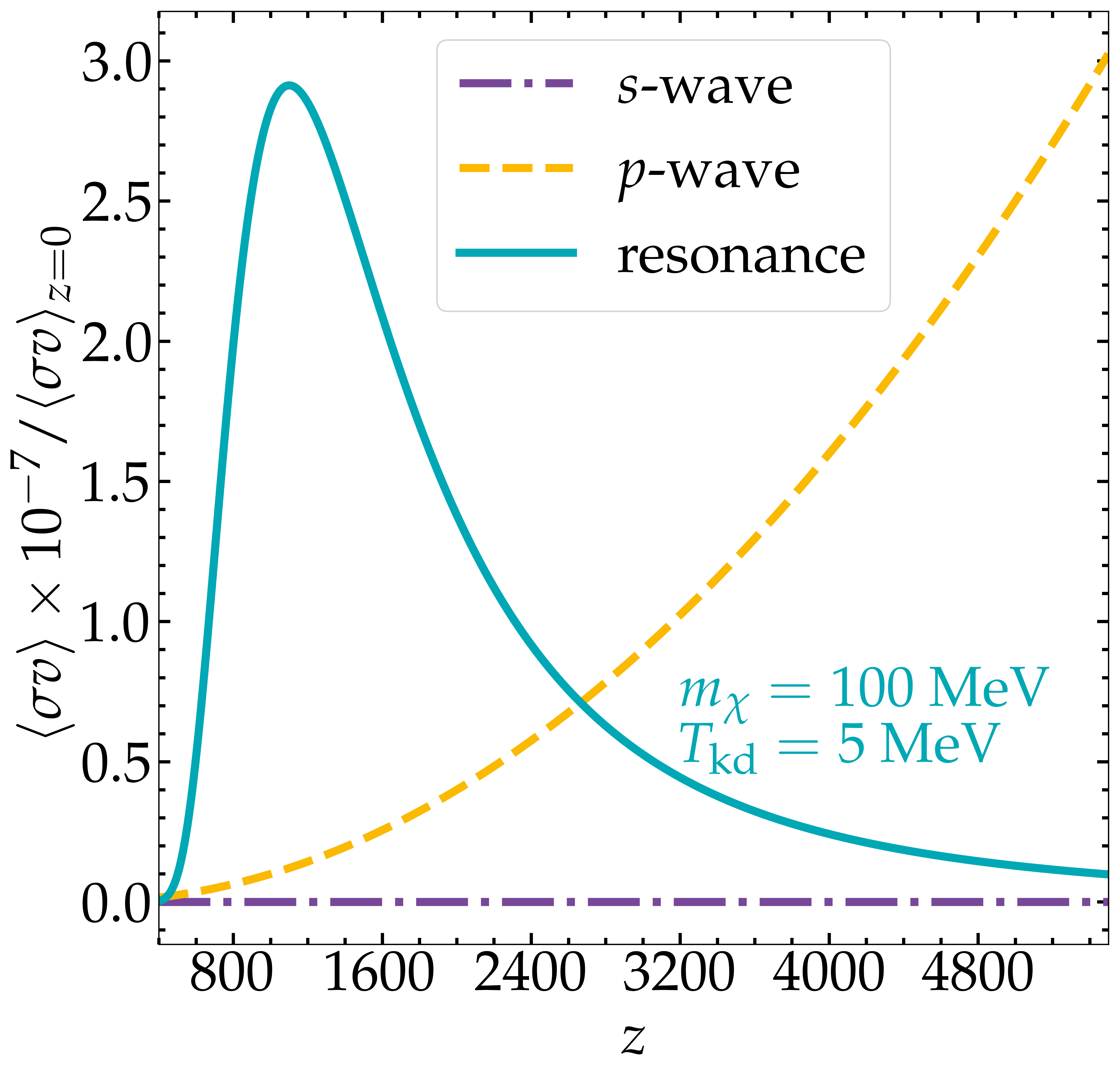
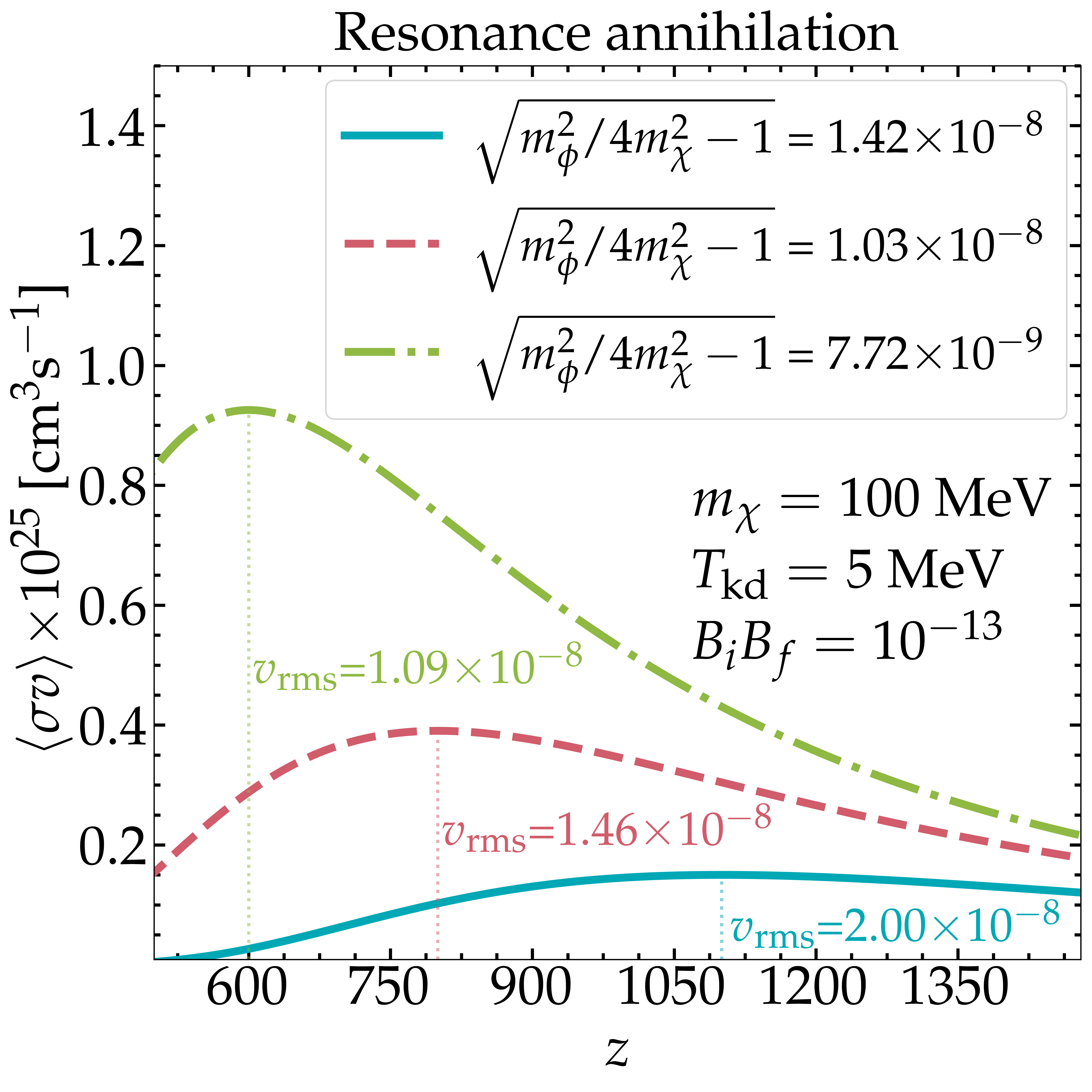
  Figure 1: The evolution of annihilation cross-section for a comparison between three scenarios (left panel) and three different $z_{\rm peak}$ benchmarks in the resonance scenario (right panel). Left panel: Thermal averaged cross-section $\langle\sigma v_{\text{rel}}\rangle$ normalized to the cross-section at $z=0$, with respect to redshift. The free parameters associated with $s$-wave and $p$-wave interactions are eliminated, while the resonance scenario is characterized by $m_{\chi}=100~\text{MeV}$ and $T_{\text{kd}}=5~\text{MeV}$. Right panel: The dash-dotted, dashed, and solid lines represent $z_{\text{peak}}=\{600,800,1100\}$, respectively. The benchmark $z_{\text{peak}}=1100$ (cyan solid lines) corresponds to the least energy injection.

• Resonance annihilation:
  For an annihilation $\chi\chi\to\phi\to f\bar{f}$ where the SM fermion is denoted as $f$, the cross-section with resonance condition $2m_{\chi}\approx m_{\phi}$ can be well described by the Breit-Wigner formula Ibe et al. (2009),

  $$\sigma=\frac{16\pi}{E^{2}_{\text{cm}}\bar{\beta_{i}}\beta_{i}}\frac{m_{\phi}^{2}\Gamma_{\phi}^{2}}{(E^{2}_{\text{cm}}-m_{\phi}^{2})^{2}+m_{\phi}^{2}\Gamma_{\phi}^{2}}B_{i}B_{f},$$ (2)

  where $E_{\text{cm}}$ is the center-of-mass energy, while $\Gamma_{\phi}$ is the decay width of the mediator $\phi$. To escape from the constraints from Big Bang Nucleosynthesis (BBN), we set $\Gamma_{\phi}=10^{-21}~\text{MeV}$, corresponding to the life time $\tau_{\phi}\sim 1$ sec. The initial state phase space factors are given by $\bar{\beta_{i}}=\sqrt{1-4m_{\chi}^{2}/m_{\phi}^{2}}$ and $\beta_{i}=\sqrt{1-4m_{\chi}^{2}/E_{\text{cm}}^{2}}$, while the decay branching ratios for $\phi\to\chi\chi$ and $\phi\to f\bar{f}$ are denoted as $B_{i}$ and $B_{f}$, respectively. For convenience, we introduce a parameter $\xi$ to describe the resonance, defined by

  $$m_{\phi}^{2}=4m_{\chi}^{2}(1+\xi),~{\rm with}~\xi\ll 1.$$ (3)

  We can see that $\xi>0$ implies $m_{\phi}>2m_{\chi}$. Using Eq. (3) and $\gamma\equiv\Gamma_{\phi}/m_{\phi}$, we can further rewrite Eq. (2) as

  $$\sigma=\frac{16\pi}{m_{\phi}^{2}\bar{\beta_{i}}\beta_{i}}\frac{\gamma^{2}}{(-\xi+v_{\text{rel}}^{2}/4)^{2}+\gamma^{2}}B_{i}B_{f}.$$ (4)

  Considering that DM are non-relativistic at the resonance, we can adopt the Maxwell-Boltzmann velocity distribution for DM to compute the velocity-averaged annihilation cross-section

  $$\langle\sigma v_{\text{rel}}\rangle=\frac{1}{(2\pi v^{2}_{\text{rms}}/3)^{3}}\int\text{d}\vec{v}_{1}\int\text{d}\vec{v}_{2}~e^{-3(v_{1}^{2}+v_{2}^{2})/(2v^{2}_{\text{rms}})}\times\sigma\times\left|\vec{v}_{1}-\vec{v}_{2}\right|,$$ (5)

  where the root-mean-square velocity $v_{\text{rms}}^{2}=\langle v^{2}_{\chi}\rangle=3T_{\chi}/m_{\chi}$ derived in (19). Since the energy injection from the non-resonant component is negligible, we focus on the velocity-averaged cross-section near resonance. By applying the narrow width approximation, we derive the velocity-averaged cross-section near resonance (see App. B for details),

  $$\langle\sigma v_{\text{rel}}\rangle=\frac{576}{\sqrt{3}}\frac{\pi^{3/2}}{m_{\phi}^{2}}\frac{\gamma}{v^{3}_{\text{rms}}}\exp{[-3\xi/v^{2}_{\text{rms}}}]B_{i}B_{f}.$$ (6)

  Interestingly, together with Eq. (1), we notice the peak of Eq. (6) located at

  $$z_{\text{peak}}=\frac{\sqrt{2\xi}}{4.07\times 10^{-10}}\sqrt{\Big{(}\frac{m_{\chi}}{1~\text{MeV}}\Big{)}\Big{(}\frac{T_{\text{kd}}}{1~\text{MeV}}\Big{)}}.$$ (7)

  Therefore, once $z_{\rm peak}$ is fixed, the remaining free parameters for the $\phi$ resonance scenario are {$m_{\chi}$, $T_{\rm kd}$, and $B_{i}B_{f}$}, where we treat $B_{i}B_{f}$ as a single combined parameter in this work.

In Fig. 1, we compare the evolution of the annihilation cross-section for three scenarios in the left panel and for three different $z_{\rm peak}$ benchmarks of the resonance scenario in the right panel. In the left panel, we normalize $\langle\sigma v_{\text{rel}}\rangle$ by its value at $z=0$, thus the $s$-wave scenario (purple dash-dotted line) indicates $\langle\sigma v_{\text{rel}}\rangle/\langle\sigma v_{\text{rel}}\rangle_{z=0}=1$, while $\langle\sigma v_{\text{rel}}\rangle/\langle\sigma v_{\text{rel}}\rangle_{z=0}=(1+z)^{2}$ is obtained by the $p$-wave scenario (yellow dashed line). Intuitively, the $p$-wave scenario is expected to be easier to detect at larger $z$. The cyan solid line represents the resonance scenario with $z_{\rm peak}=1100$. Clearly, if $z_{\rm peak}$ occurs during the recombination epoch, the resonance scenario offers a more promising detection prospect than the other two.

In the right panel, we illustrate the resonance scenario with $m_{\chi}=100\,\mathrm{MeV}$, $T_{\rm kd}=5\,\mathrm{MeV}$, and $B_{i}B_{f}=10^{-13}$ as an example. We present three benchmarks: $z_{\text{peak}}=600$ (green dash-dotted line), $z_{\text{peak}}=800$ (red dashed line), and $z_{\text{peak}}=1100$ (cyan solid line), corresponding to $v_{\rm rms}=1.09\times 10^{-8}$, $v_{\rm rms}=1.46\times 10^{-8}$, and $v_{\rm rms}=2.0\times 10^{-8}$, respectively.

We find that achieving resonance in the range $600<z_{\rm peak}<1100$ requires fine-tuning value of $\xi\sim\mathcal{O}(10^{-16})$, which is challenging for DM indirect detection due to the larger DM velocity, $\xi\approx 10^{-6}$.

II.2 Energy Deposition

When DM particles annihilate into primary particles, such as SM particles and long-lived new particles, these can decay into stable particles and inject energy into the universe, while neutrino final states do not contribute to gas heating or ionization. For DM masses from a few MeVs to a few GeVs, possible annihilation channels include two-body final states (e.g., $2e^{\pm}$, $2\mu^{\pm}$, or $2\pi$) or four-body final states (e.g., $4e^{\pm}$, $4\mu^{\pm}$, or $4\pi$), which arise from the decay of two long-lived new particles. However, Planck constraints on four-body models are similar to those on two-body models across a wide DM mass range, as the constraints are mainly sensitive to the total energy of $e^{\pm}$ and $\gamma$ final states, not their spectrum shapes Clark et al. (2017). In this work, we focus on two-body final states (electron-positron pairs and pions), since electrons and positrons are leptons, while pions are mesons made of up and down quarks. For simplicity, we adopt the Higgs portal model to compute the pion branch ratios, $\text{BR}(\chi\chi\rightarrow\pi^{+}\pi^{-})=2/3$ and $\text{BR}(\chi\chi\rightarrow\pi^{0}\pi^{0})=1/3$.

We compute DM energy deposition energy that goes into ionization, heating and excitation of the IGM, as

$$\bigg{(}\frac{\text{d}E}{\text{d}V~\text{d}t}\bigg{)}^{\text{dep}}_{c}=f_{c}(z,\mathbf{x})\bigg{(}\frac{\text{d}E}{\text{d}V~\text{d}t}\bigg{)}^{\text{inj}},$$ (8)

where the energy injections induced by DM annihilation are

$$\bigg{(}\frac{\text{d}E}{\text{d}V~\text{d}t}\bigg{)}^{\text{inj}}=\Omega_{\chi}^{2}\rho_{\rm crit}^{2}(1+z)^{6}\langle\sigma v_{\text{rel}}\rangle/m_{\chi},$$ (9)

where $V$ is comoving volume, $t$ is physical time, $\Omega_{\chi}$ is DM density parameter of today, $\rho_{\rm crit}$ is the critical density of today. The index $c=\{\text{HI, heat, Ly}\alpha\}$ denotes hydrogen ionization, heating, or Ly$\alpha$ excitation channels. The deposition function $f_{c}(z,\mathbf{x})$, dependent on redshift $z$ and ionization fractions $\mathbf{x}\equiv\{x_{\text{HII}},x_{\text{HeII}},x_{\text{HeIII}}\}$, is computed via DarkHistory Liu et al. (2023a, b) using photon and electron spectra from DM annihilation generated by Hazma Coogan et al. (2020b).

The impact of energy injection from DM annihilation on the ionization history is given in Ref. Liu et al. (2020) by the following equations:

$$\dot{T}^{\text{inj}}_{m} =\frac{2f_{\text{heat}}(z,\textbf{x})}{3(1+\mathcal{F}_{\text{He}}+x_{e})n_{\text{H}}}\left(\frac{\text{d}E}{\text{d}V~\text{d}t}\right)^{\text{inj}},$$ (10)

$$\dot{x}^{\text{inj}}_{\text{HII}} =\left[\frac{f_{\text{ion}}(z,\mathbf{x})}{\mathcal{R}n_{\text{H}}}+\frac{(1-\mathcal{C})f_{\text{exc}}(z,\mathbf{x})}{0.75\mathcal{R}n_{\text{H}}}\right]\left(\frac{\text{d}E}{\text{d}V~\text{d}t}\right)^{\text{inj}},$$

where $\mathcal{F}_{\text{He}}\equiv n_{\text{He}}/n_{\text{H}}$ is the helium-to-hydrogen ratio, and $n_{\text{He}}$ and $n_{\text{H}}$ are the number densities of helium and hydrogen (both neutral and ionized), respectively. The ionization potential of hydrogen is $\mathcal{R}=13.6~\text{eV}$, and $\mathcal{C}$ is the Peebles C factor, which represents the probability of a hydrogen atom in the $n=2$ state decaying to the ground state before photoionization occurs Ali-Haïmoud and Hirata (2011); Peebles (1968).

We use DarkHistory v2.0 Liu et al. (2023a, b), which improves the treatment of low-energy photons and electrons compared to DarkHistory v1.0 Liu et al. (2020), to compute additional energy injection from DM annihilation into the universe thermal and ionization evolution. After tabulating the results of Eq. (10), we insert them into CLASS Lesgourgues (2011a); Blas et al. (2011); Lesgourgues (2011b); Lesgourgues and Tram (2011) to calculate the CMB power spectra and blackbody spectral distortions.

III Constraints from CMB

This section aims to briefly outline the CMB constraints and the statistical framework used to explore the parameter space of three benchmark scenarios.

III.1 Blackbody spectral distortions

In the early universe, photons are thermalized efficiently because of rapid interactions with baryons, including double Compton scattering ($e^{-}+\gamma\rightarrow e^{-}+\gamma+\gamma$), bremsstrahlung ($e^{-}+N\rightarrow e^{-}+N+\gamma$), and Compton scattering ($\gamma+e^{-}\rightarrow\gamma+e^{-}$), which leads to blackbody spectral distortions

$$I(E_{\gamma},T_{z})=\frac{E_{\gamma}^{3}}{\pi^{3}}\frac{1}{e^{E_{\gamma}/T_{z}}-1}\propto\frac{1}{e^{x}-1},\,$$ (11)

where $x\equiv E_{\gamma}/T_{z}$ and $T_{z}\equiv T_{\text{CMB,0}}(1+z)$ represent the reference temperature in equilibrium with the thermal bath. In an expanding universe, above interactions weaken over time and become insufficient before recombination, allowing DM-induced energy injections to leave imprints on the CMB frequency spectrum Chluba (2013a); Lucca et al. (2020); Lucca (2023); Li (2024).

As $z\mathrel{\mathop{\kern 0.0pt\hbox to0.0pt{\raise 0.86108pt\hbox{$<$}\hss}}\lower 3.87495pt\hbox{\kern-1.90002pt$\sim$}}z_{\text{th}}\approx 2\times 10^{6}$, the injected energy cannot fully thermalize, and the processes changing the number density such as double Compton scattering and bremsstrahlung become inefficient. The chemical potential of photons becomes non-zero, proportional to the energy deposit, which creates $\mu$-distortion. By perturbating the blackbody spectrum Eq. (11), the $\mu$-distortion of CMB is defined as follows,

$$I(E_{\gamma},x;\mu)=\frac{E_{\gamma}^{3}}{\pi^{3}}\frac{1}{e^{x+\mu}-1}\simeq\frac{E_{\gamma}^{3}}{\pi^{3}}\left(\frac{1}{e^{x}-1}-\mu\frac{e^{x}}{(e^{x}-1)^{2}}\right).\,$$ (12)

The $\mu$-distortion from energy injection of DM annihilation is evaluated from Green’s function method Chluba (2013b, 2015)

$$\mu\simeq-1.401\int_{z_{\mu}}^{z_{\mu y}}\frac{1}{\rho_{\gamma}(z)}\bigg{(}\frac{\text{d}E}{\text{d}V~\text{d}t}\bigg{)}^{\text{inj}}\frac{1}{(1+z)H(z)}\cdot\mathcal{J}_{\mu}(z)\text{d}z,$$ (13)

where $\rho_{\gamma}\approx 0.26(1+z)^{4}~\text{eV/cm}^{3}$. The Green’s function is evaluated as

$$\mathcal{J}_{\mu}(z)\simeq\left\{1-\exp{\left[-\left(\frac{1+z}{5.8\times 10^{4}}\right)^{1.88}\right]}\right\}\exp{\left[-\left(\frac{z}{z_{\text{th}}}\right)^{5/2}\right]}.$$

Since the universe is fully ionized, and energy injection follows the on-the-spot approximation Padmanabhan and Finkbeiner (2005a). Under such an assumption, DM annihilation into photons and electrons results in instantaneous and complete energy deposition into heating the IGM.

When $z\mathrel{\mathop{\kern 0.0pt\hbox to0.0pt{\raise 0.86108pt\hbox{$<$}\hss}}\lower 3.87495pt\hbox{\kern-1.90002pt$\sim$}}z_{\mu y}\approx 5\times 10^{4}$, Compton scattering as well as energy redistribution become inefficient, driving photons away from Bose-Einstein distribution, which creates $y$-distortion. However, for DM annihilation, the cross-section with positive power of velocity dependence decreases with time. In these scenarios, more energy injects into the background during $\mu$-distortion era than $y$-distortion era, which may lead to more stringent constrain on the parameter space Li (2024). Therefore, we only consider $\mu$-distortion in this work.

The FIRAS experiment was aboard the COBE satellite provided one of the most precise measurements of the CMB spectrum. It has reported $|\mu|<4.7\times 10^{-5}$ Bianchini and Fabbian (2022), improving the previous monopole $\mu$-distortion limit $|\mu|<9\times 10^{-5}$ Fixsen et al. (1996b), due to more robust foreground cleaning.

Future missions aim to refine these limits and potentially detect smaller distortions. The 95% upper limit for $\mu$ from PRISTINE will be $|\mu|<8\times 10^{-7}$ Chluba et al. (2019), while PIXIE (Primordial Inflation Explorer) will set a more stringent limit of $|\mu|<8\times 10^{-8}$ Chluba et al. (2019) at the same confidence level.

III.2 CMB anisotropies

spectrum because it enhances the visibility of reionization-induced polarization Padmanabhan and Finkbeiner (2005a).

DM annihilation produces high-energy photons and electrons that heat and ionize hydrogen gas, broadening the last scattering surface. This increases the residual free electron fraction after recombination, enhancing Thomson scattering. As a result, the damping tail of the CMB temperature power spectrum at small angular scales is suppressed due to photon redistribution Padmanabhan and Finkbeiner (2005b); Galli et al. (2009); Slatyer et al. (2009). Furthermore, increased ionization at later times boosts the low-$l$ polarization power spectrum by enhancing the visibility of reionization-induced polarization Padmanabhan and Finkbeiner (2005a).

As shown in Ref. Huang et al. (2021), the current Planck 2018 angular power spectra data Aghanim et al. (2020a) is particularly sensitive to DM-induced energy injection in the redshift range of 600 to 1000. This Planck data includes the baseline high-$l$ power spectra (TT, TE, and EE), the low-$l$ power spectrum TT, the low-$l$ HFI polarization power spectrum EE, and the lensing power spectrum. For $s$-wave annihilation with DM masses between MeV and GeV, the CMB angular power spectrum constraints are significantly stronger than those from DM indirect detection. In addition, Refs. Slatyer et al. (2009); Slatyer (2016) indicate that $f_{c}(z,\mathbf{x})$ in this redshift range can be approximated as a constant. Consequently, for $s$-wave annihilation, an effective parameter constrained by CMB anisotropies is defined as $p_{\rm eff}\equiv f_{c}(z,\mathbf{x})\langle\sigma v_{\text{rel}}\rangle/m_{\chi}^{2}$, with the Planck 95% upper limit of $p_{\rm eff}<3.2\times 10^{-28}\,\text{cm}^{3}\,\text{s}^{-1}\,\text{GeV}^{-1}$ (Planck TT+TE+EE+lowE+lensing+BAO) Aghanim et al. (2020a). However, these simplifications are not accurate when considering a velocity-dependent annihilation cross-section. Therefore, based on the current Planck data and the future prospects of LiteBird Suzuki et al. (2018) and CMB-S4 Abazajian et al. (2016, 2019), we derive comprehensive limits for $p$-wave and resonance annihilation scenarios in this work.

III.3 Statistical framework

In this work, we utilize two types of likelihood distributions in the analysis. For blackbody spectral distortions, we adopt the 95% upper limit, $|\mu|<4.7\times 10^{-5}$, from FIRAS, meaning that the likelihood probabilities for a predicted $|\mu|$ exceeding $4.7\times 10^{-5}$ are zero. Similarly, we apply upper limits to the likelihoods for all future experimental prospects, including the future measurements of blackbody spectral distortions and CMB anisotropies. For data measurements, such as the CMB angular power spectra (TT, TE, and EE), we use Gaussian likelihoods included in the numerical MontePython Brinckmann and Lesgourgues (2018). To complete the likelihoods for CMB anisotropies, we incorporate the Planck 2018 data Aghanim et al. (2020a), including high-$\ell$ (TT, TE, EE) spectra, low-$\ell$ temperature TT spectrum, low-$\ell$ polarization EE spectrum, lensing power spectrum, and BAO data Alam et al. (2017); Buen-Abad et al. (2018); Beutler et al. (2011); Ross et al. (2015).

To present our results, we use two statistical methods: the “marginal posterior” (MP) method and the “profile likelihood” (PL) method. The MP approach integrates the probability density over nuisance parameters by marginalizing the posterior, commonly used in cosmology, especially within the $\Lambda$CDM framework. In contrast, the PL method is preferred for null signal searches due to large volume effects and prior dependencies in unconstrained likelihoods, and is widely applied in DM direct and indirect detection. For the MP method, we use the prior distributions as described in Ref. Lewis (2013) on six cosmological parameters as nuisances—$\{\Omega_{b}h^{2},\Omega_{\text{CDM}}h^{2},100\theta_{s},\log(10^{10}A_{s}),n_{s},\tau_{\text{reio}}\}$—informed by Planck precise central values and uncertainties. However, we apply log priors for $\langle\sigma v_{\text{rel}}\rangle$, $b$, and $B_{i}B_{f}$ for three scenarios, respectively. For the PL method, we perform several fine scans in addition to the original Bayesian scan to improve coverage. For both methods, we exclude parameter regions where the accumulated probability exceeds 95% for each fixed $m_{\chi}$.

IV Numerical results

	redshift $z$	$s$-wave	$p$-wave	resonance
$\mu$-distortion	$5\times 10^{4}\mathrel{\mathop{\kern 0.0pt\hbox to0.0pt{\raise 0.86108pt\hbox{$<$}\hss}}\lower 3.87495pt\hbox{\kern-1.90002pt$\sim$}}z\mathrel{\mathop{\kern 0.0pt\hbox to0.0pt{\raise 0.86108pt\hbox{$<$}\hss}}\lower 3.87495pt\hbox{\kern-1.90002pt$\sim$}}2\times 10^{6}$		$\checkmark$
CMB anisotropies	$600\mathrel{\mathop{\kern 0.0pt\hbox to0.0pt{\raise 0.86108pt\hbox{$<$}\hss}}\lower 3.87495pt\hbox{\kern-1.90002pt$\sim$}}z\mathrel{\mathop{\kern 0.0pt\hbox to0.0pt{\raise 0.86108pt\hbox{$<$}\hss}}\lower 3.87495pt\hbox{\kern-1.90002pt$\sim$}}1100$	$\checkmark$		$\checkmark$

Table 1: Comparison of constraint power between FIRAS $\mu$-distortion and Planck CMB anisotropies. Note that the $y$-distortion constraint is weaker than those from $\mu$-distortion or CMB anisotropies.

We compare the 95% upper limits on $\mu$-distortion and $y$-distortion from FIRAS with those from CMB anisotropies in Planck. We find that $\mu$-distortion provides a more stringent constraint only for $p$-wave annihilation, due to its larger cross-section at higher redshifts ($5\times 10^{4}\lesssim z\lesssim 2\times 10^{6}$). Therefore, we omit the $y$-distortion analysis. For the resonance scenario, we set the resonance peaks for $\mu$-distortion at $z_{\text{peak}}=10^{6}$ and $y$-distortion at $z_{\text{peak}}=10^{4}$, with DM parameters $m_{\chi}=1~\text{GeV}$, $T_{\text{kd}}=m_{\chi}/3$, and $B_{i}B_{f}=0.25$ (which yields a larger cross-section for comparison). However, we find that the resonance effect on the distortion is negligible, as the resonance redshift range is much narrower than that of the distortions, resulting in minimal energy injection. The most stringent limits for the three annihilation scenarios are summarized in Tab. 1.

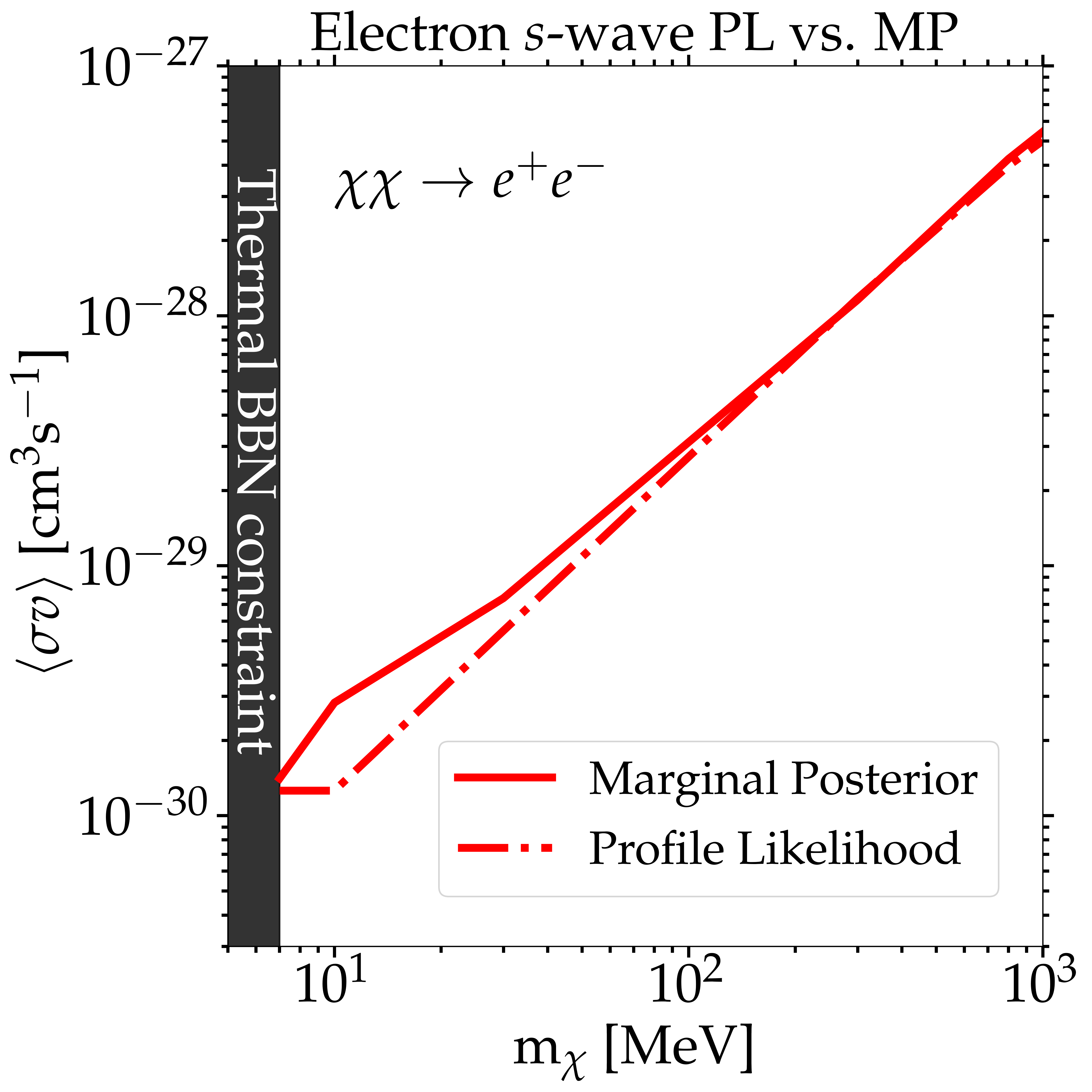
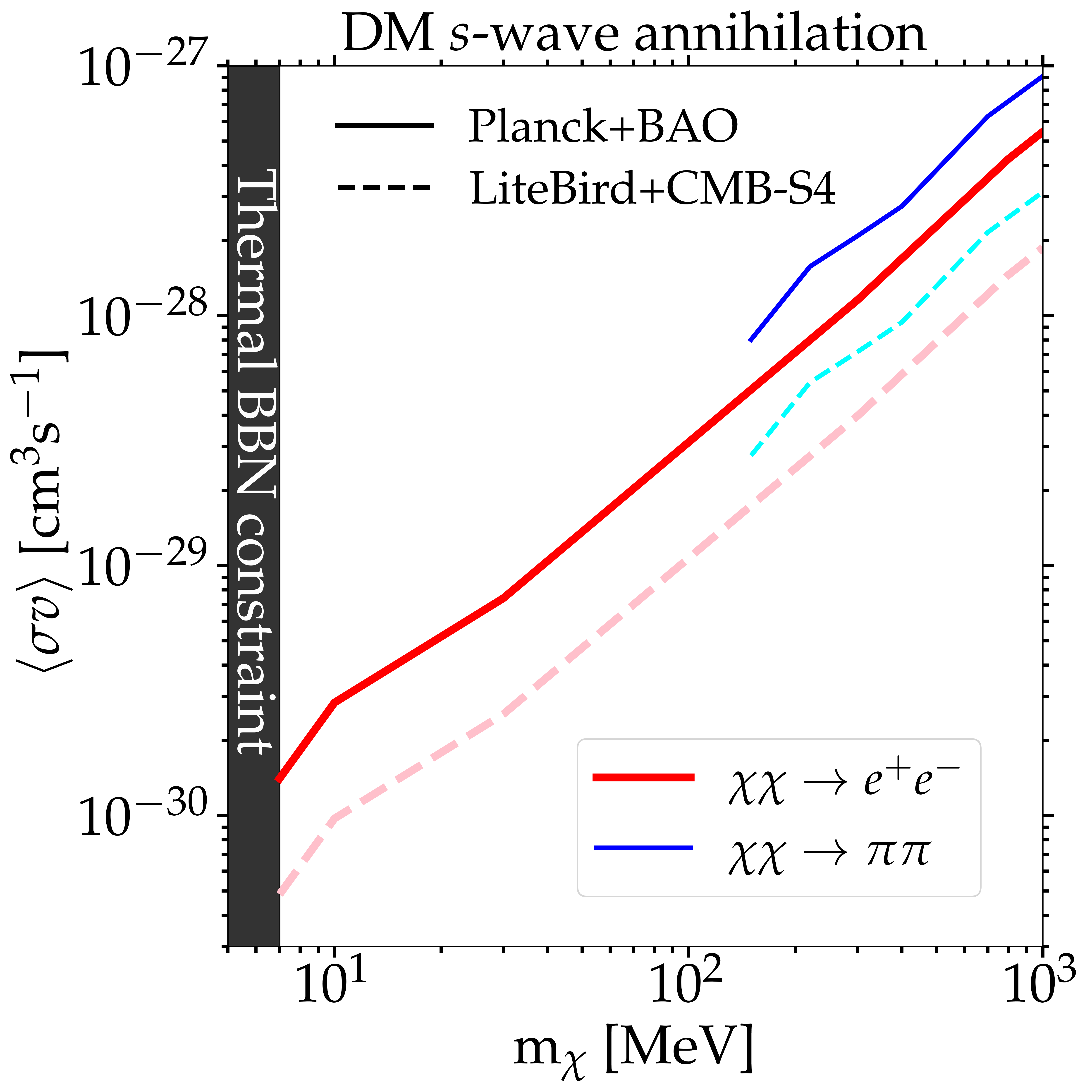
Figure 2: Comparison of the 95% upper limits on $\langle\sigma v_{\text{rel}}\rangle$ for $s$-wave annihilation based on the Planck+BAO likelihood. The left panel shows limits from the MP (red solid line) and PL (red dash-dotted line) methods for $e^{+}e^{-}$ final state. The right panel compares the $e^{+}e^{-}$ (red) and $\pi\pi$ (blue) final states for Planck+BAO (solid lines) and future LiteBird and CMB-S4 experiments Fu et al. (2021).

Fig. 2 displays the 95% upper limits on the ($m_{\chi}$, $\langle\sigma v_{\text{rel}}\rangle$) plane for the $s$-wave annihilation scenario, derived from the Planck+BAO likelihood. In the left panel, the limits for the $e^{+}e^{-}$ final state are compared between PL (red dash-dotted line) and MP (red solid line) method. The right panel compares the $e^{+}e^{-}$ (red) and $\pi\pi$ (blue) final states for the Planck+BAO likelihood (dark color) and the future LiteBird and CMB-S4 prospects Fu et al. (2021) (light color). The black regions indicate the BBN exclusion of thermal DM particles with masses below $7\,\mathrm{MeV}$ Depta et al. (2019); Sabti et al. (2021). Hence, we set $7\,\mathrm{MeV}$ as the lower mass limit for the electron channel.

The left panel of Fig. 2 shows that the PL result is stronger than the MP result, as expected. The MP method averages over all parameters, smoothing out nuisance effects and leading to less stringent constraints. In contrast, the PL method maximizes the likelihood for each parameter, providing sharper and more stringent limits on $\langle\sigma v_{\text{rel}}\rangle$. In the right panel of Fig. 2, a lower mass limit of 150 MeV is set for the $\pi\pi$ final state, based on the rest mass of the $\pi^{\pm}$ (139.57 MeV) and $\pi^{0}$ (134.98 MeV). Our $e^{+}e^{-}$ limits agree with previous studies Cang et al. (2020), while future experiments improve the constraints by approximately a factor of around 3. Note that blackbody spectral distortions limits are not as powerful as the Planck+BAO likelihood for probing the $s$-wave annihilation, even with the most advanced future blackbody spectral distortions missions Chluba (2013a); Fu et al. (2021).

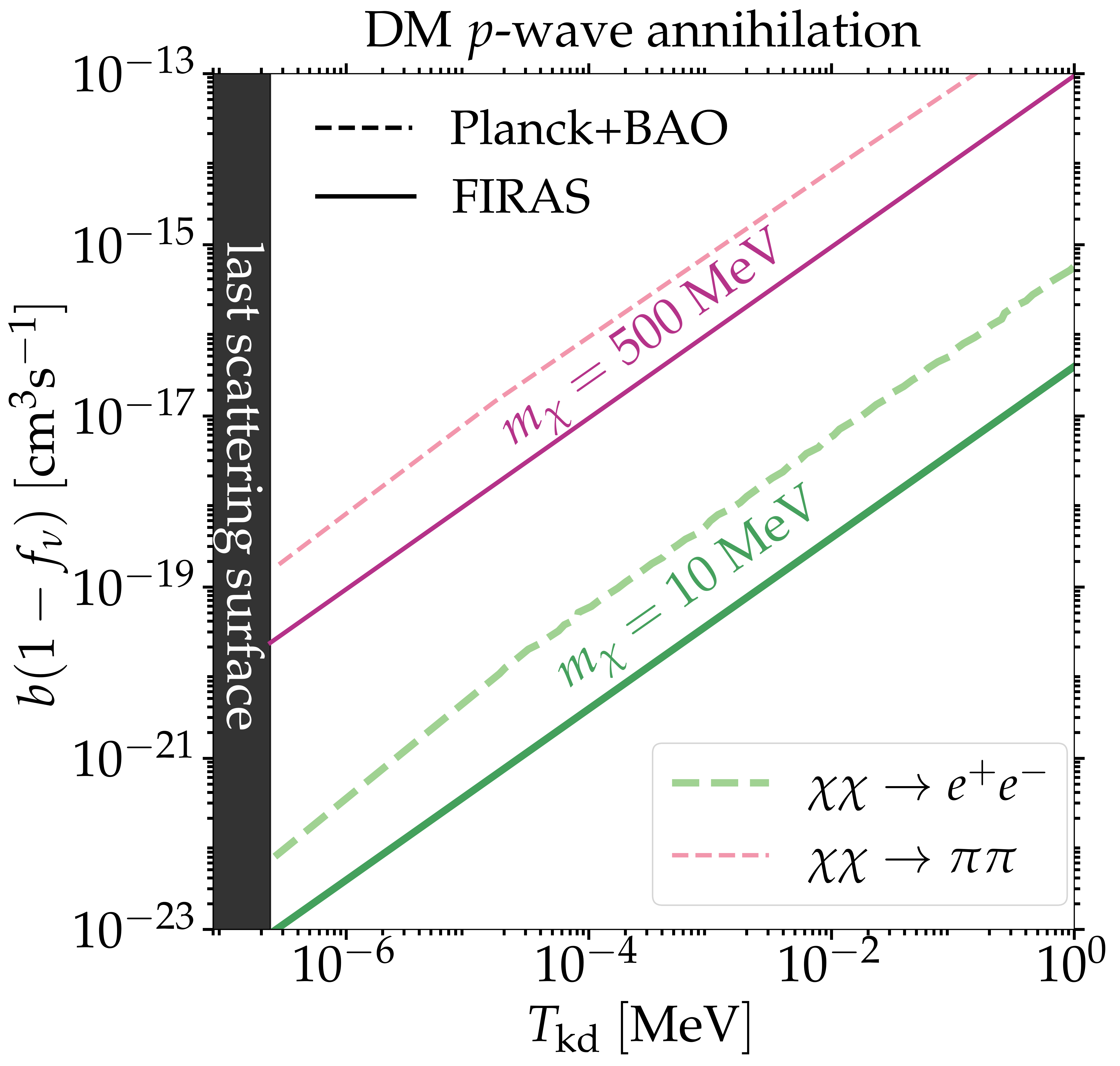
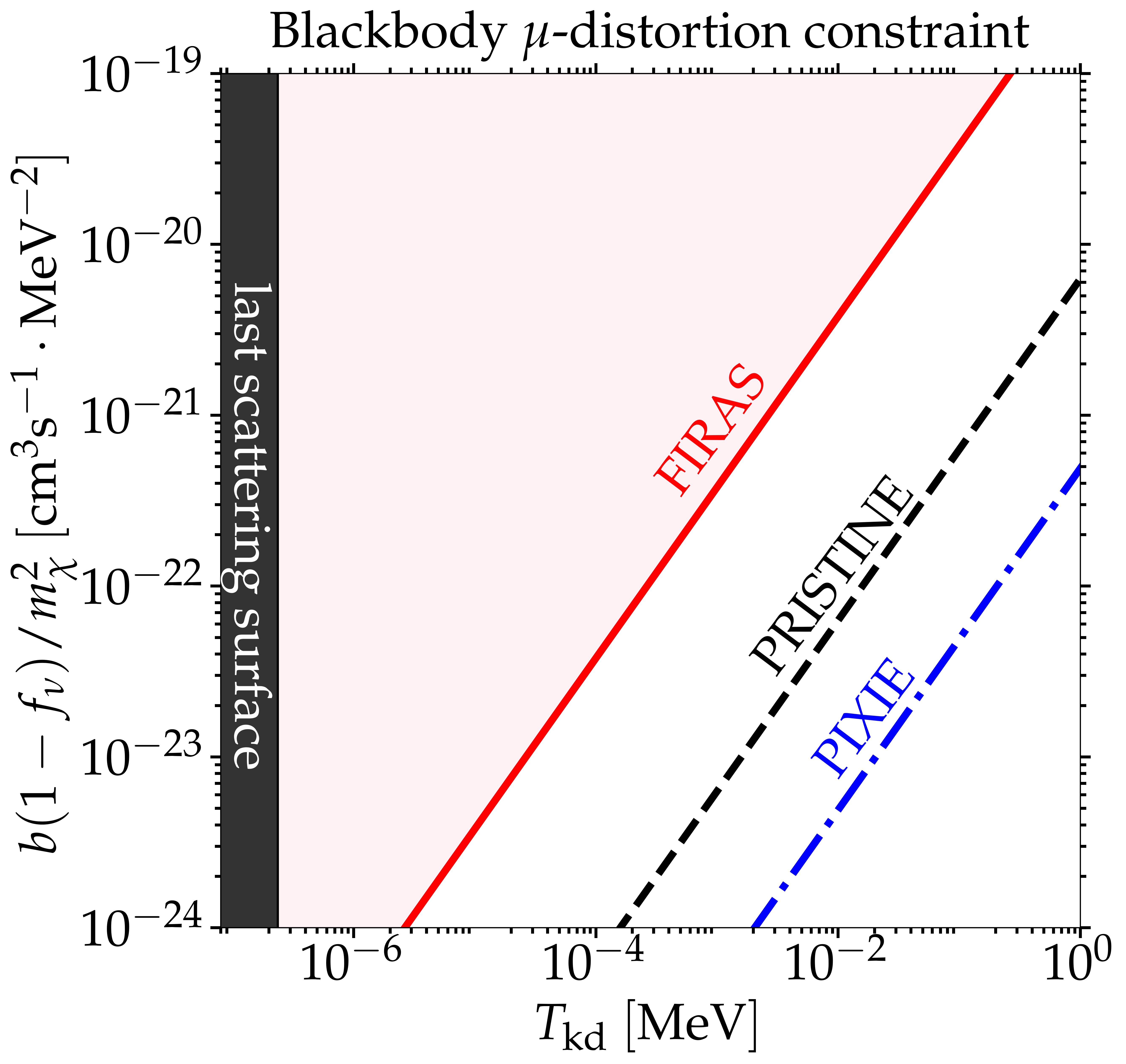
Figure 3: The upper limits projected on the $T_{\rm kd}$ versus $b(1-f_{\nu})$) plane (left) and the $T_{\rm kd}$ versus $b(1-f_{\nu})/m_{\chi}^{2}$ plane (right). The black region represents the last scattering surface, assuming kinetic decoupling occurs after chemical decoupling but before the CMB. The solid lines show the 95% upper limit of FIRAS $\mu$-distortion constraints for $m_{\chi}=10\,\mathrm{MeV}$ (green line) and $m_{\chi}=500\,\mathrm{MeV}$ (magenta line). Their corresponding dashed lines represent the 95% upper limits of $b(1-f_{\nu})$ derived from the Planck+BAO likelihood, by using the MP method. In the right panel, the red solid, black dashed, and blue dash-dotted lines represent the FIRAS, PRISTINE, and PIXIE the 95% upper limit of $\mu$-distortion constraints, respectively.

Fig. 3 shows the constraints for $p$-wave DM annihilation. The left panel displays the relation between $T_{\rm kd}$ and $b(1-f_{\nu})$, while the right panel shows $T_{\rm kd}$ versus $b(1-f_{\nu})/m_{\chi}^{2}$. Here, $f_{\nu}$ is the fraction of DM annihilation energy that goes into neutrinos. For DM annihilation into $e^{+}e^{-}$, $f_{\nu}$ is zero, while for charged pions, $f_{\nu}$ approximates to $0.47$. The black region represents the last scattering surface, assuming kinetic decoupling occurs after chemical decoupling but before the CMB epoch. In the left panel, the FIRAS $\mu$-distortion constraints (solid lines) are stronger than those from the Planck+BAO likelihood (dashed lines), as the $p$-wave cross-section increases with redshift, making the $\mu$-distortion constraint stronger than the $y$-distortion one Li (2024). Similarly, BBN and light-element abundances can yield stronger limits than the FIRAS constraints. However, future missions like PIXIE and Super-PIXIE will surpass BBN limits Braat and Hufnagel (2024). The green and magenta lines show the 95% upper limits for $e^{+}e^{-}$ ($m_{\chi}=10\,\mathrm{MeV}$) and $\pi\pi$ ($m_{\chi}=500\,\mathrm{MeV}$), respectively. Both solid and dashed lines are derived by the MP method. Although the PL result is stronger than the MP result, it remains weaker than the FIRAS constraints.

The right panel of Fig. 3 illustrates the relation between $T_{\rm kd}$ and $b(1-f_{\nu})/m_{\chi}^{2}$, derived from the $\mu$-distortion constraints for DM $p$-wave annihilation. Due to the linearity of upper limits, we can parameterize the 95% constraints from FIRAS, PRISTINE, and PIXIE as

$$\frac{T_{\text{kd}}}{1~\text{MeV}}\geq h_{i}\times b\times(1-f_{\nu})\times\left(\frac{1~\text{MeV}}{m_{\chi}}\right)^{2},$$ (14)

where $i=\{\text{FIRAS,~PRISTINE,~PIXIE}\}$ and $h_{\text{FIRAS}}=2.643\times 10^{18}$, $h_{\text{PRISTINE}}=1.589\times 10^{20}$, and $h_{\text{PIXIE}}=2.045\times 10^{21}$. This model-independent inequality, Eq. (14), is useful for testing arbitrary $p$-wave DM models.

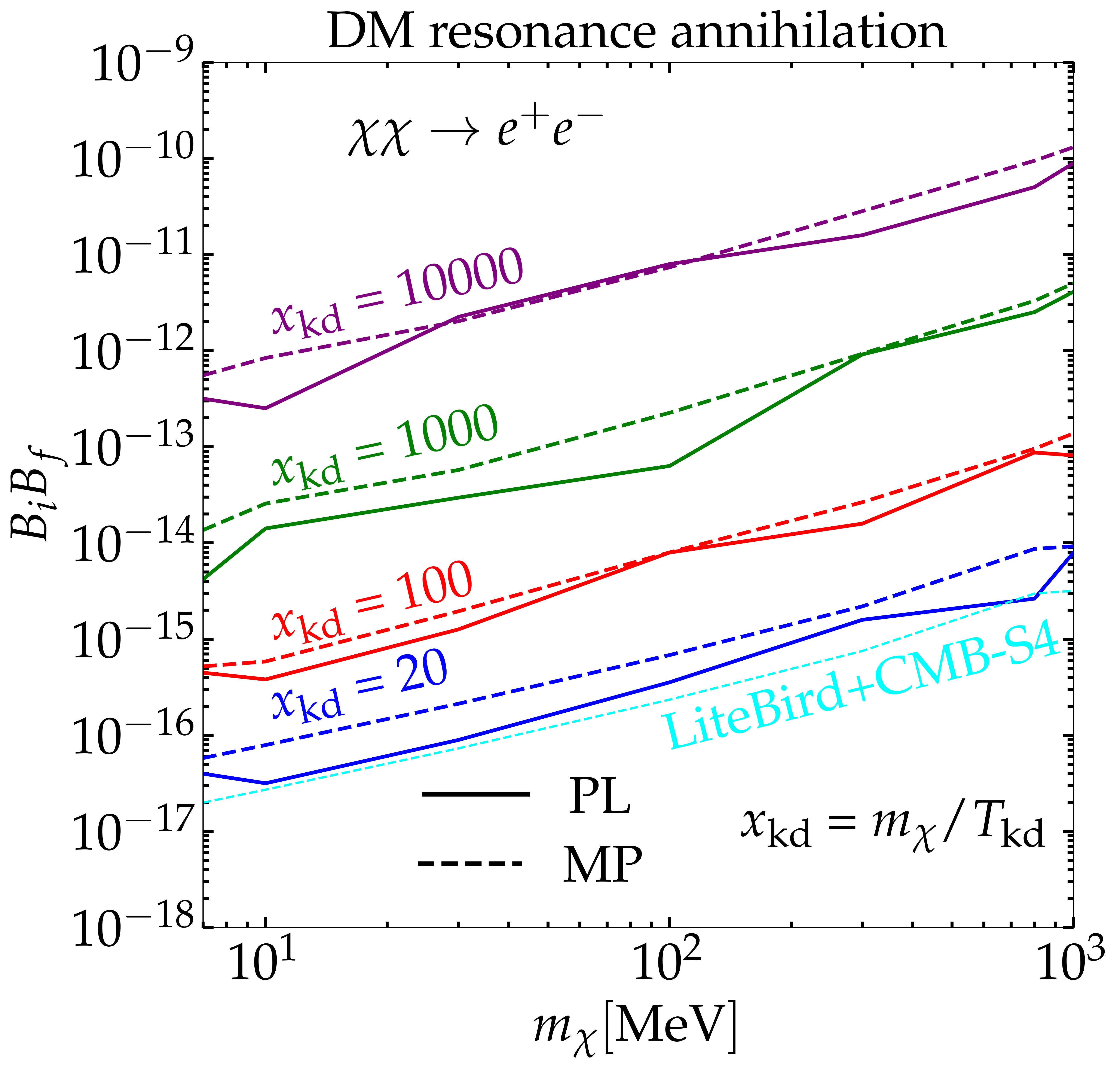
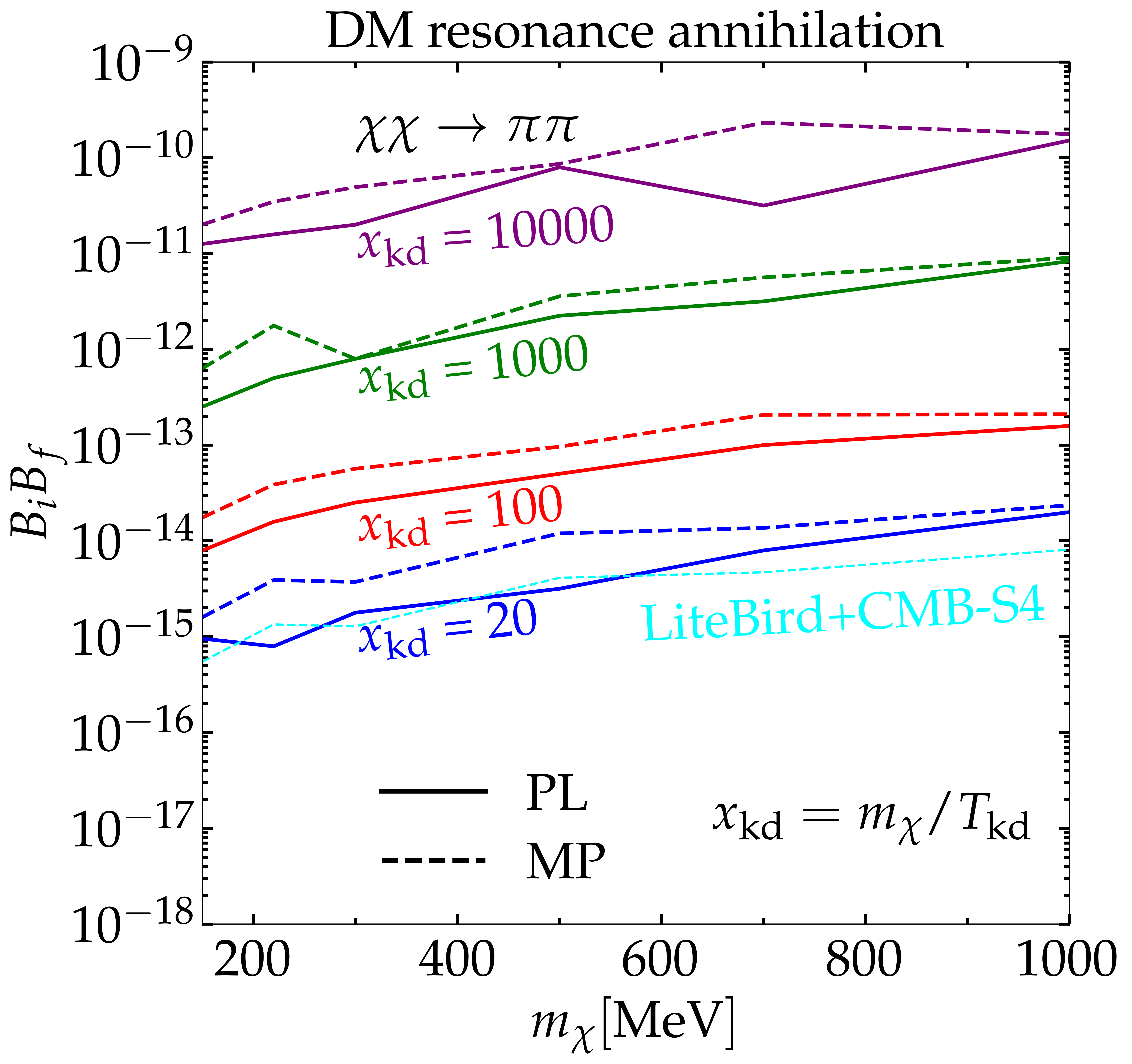
Figure 4: The $95\%$ upper limits of the DM resonance annihilation coupling coefficient, based on the Planck+BAO likelihood. The left panel shows the electron channel, while the right panel shows the pion channel. The solid lines use the PL method, and the dashed lines use the MP method. The values of $x_{\text{kd}}\equiv m_{\chi}/T_{\text{kd}}$ are $\{20,100,1000,10000\}$, from bottom to top. The thin cyan dashed lines are derived using the configurations $x_{\text{kd}}=20$, LiteBird+CMB-S4 Fu et al. (2021), and the MP method.

Fig. 4 shows the 95% upper limits on $B_{i}B_{f}$ for the resonance annihilation scenario, derived from the Planck+BAO likelihood. For a conservative approach, we fix the resonance peak at $z_{\text{peak}}=1100$, which yields the weakest limits compared to those at the range $600\leq z_{\text{peak}}<1100$, as shown in the right panel of Fig. 1. The limits are obtained using the PL method (solid lines) and the MP method (dashed lines). The left and right panels show results for $e^{+}e^{-}$ and $\pi\pi$ final states, respectively. The values of $x_{\text{kd}}\equiv m_{\chi}/T_{\text{kd}}$ are set to 20 (blue lines), $10^{2}$ (red lines), $10^{3}$ (green lines), and $10^{4}$ (purple lines). The thin cyan dashed lines are derived by future LiteBird and CMB-S4 sensitivities Fu et al. (2021) using the configurations $x_{\text{kd}}=20$ and the MP method. Note that smaller values of $x_{\text{kd}}$ correspond to earlier kinetic decoupling (larger $T_{\text{kd}}$) for the same DM mass. As shown in Eq. (7), larger $T_{\text{kd}}$ results in smaller $\xi$, which strengthens the constraints on $B_{i}B_{f}$. For reference, we compute $\langle\sigma v_{\text{rel}}\rangle$ at $1+z=z_{\text{peak}}=1100$ for a given $B_{i}B_{f}$. Taking $m_{\chi}=1\,\text{GeV}$ and $x_{\text{kd}}=20$ (blue dashed line), the upper limits $B_{i}B_{f}=9\times 10^{-15}$ (e${}^{+}e^{-}$) and $B_{i}B_{f}=2\times 10^{-14}$ ($\mu^{+}\mu^{-}$) correspond to annihilation cross-sections $\langle\sigma v_{\text{rel}}\rangle$ of $7.03\times 10^{-28}\,\text{cm}^{3}\,\text{s}^{-1}$ and $1.77\times 10^{-27}\,\text{cm}^{3}\,\text{s}^{-1}$, respectively, at $1+z=z_{\text{peak}}=1100$.

We comment on our results for $B_{i}B_{f}$ using the example of 100 MeV DM annihilation through dark Higgs into $e^{+}e^{-}$ Chen et al. (2024). For $100\,\mathrm{MeV}$ DM annihilating into $e^{+}e^{-}$ shown in Fig. 4, we obtain $B_{f}<10^{-16}$ under reasonable assumptions ($B_{i}\approx 1$ and $x_{\text{kd}}=20$). The constraints on $B_{f}$, which scale as $B_{f}\propto\sin^{2}\theta$ Chen et al. (2024), imply $\sin\theta<10^{-14}$ with $\xi=2.02\times 10^{-16}$. These limits are significantly stronger than those from the DarkSide-50 DM direct detection experiment Agnes et al. (2023), as shown in Chen et al. (2024). Note that our result in Fig. 4 assumes $z_{\text{peak}}=1100$, which provides the weakest limits compared to the case of $600\leq z_{\text{peak}}<1100$.

V Conclusion

In this work, we have systematically investigated the constraints imposed by the Planck, BAO and FIRAS likelihood on sub-GeV DM annihilation, considering both $e^{+}e^{-}$ and $\pi\pi$ final states through $s$-wave, $p$-wave, and resonance processes. The comparison of constraint strength between FIRAS $\mu$-distortion and Planck CMB anisotropies is summarized in Table 1, where we note that the $y$-distortion constraint is weaker than those from $\mu$-distortion or CMB anisotropies.

For the $s$-wave annihilation scenario, we have provided constraints for both the $e^{+}e^{-}$ and $\pi\pi$ channels. We find that the PL result is stronger than the MP result, as expected. We also further extend the analysis to include the pion channel and future experiments, such as LiteBird and CMB-S4, both derived using the MP method. Our results for the $e^{+}e^{-}$ channel agree with previous studies, while the inclusion of the $\pi\pi$ channel provides new insights into the constraints on DM annihilation with $m_{\chi}\sim\mathcal{O}(100)\,\mathrm{MeV}$.

In the $p$-wave annihilation scenario, we derived a model-independent inequality (Eq. (14)) that parameterizes the $95\%$ upper limits from FIRAS, PRISTINE, and PIXIE. The $\mu$-distortion constraints depend solely on the DM mass, not the annihilation channel, due to the on-the-spot approximation during the $\mu$-distortion redshift range ($5\times 10^{4}\lesssim z\lesssim 2\times 10^{6}$). Future experiments like PIXIE and Super-PIXIE are expected to surpass the current BBN limits, providing more stringent constraints on $p$-wave DM annihilation.

For the resonance annihilation scenario, we focused on the case where the resonance peak occurs at $z_{\rm peak}=1100$, which yields the weakest limits compared to the case of $600\leq z_{\text{peak}}<1100$. Under this assumption, we calculated the constraints on the coupling coefficient $B_{i}B_{f}$ for both $e^{+}e^{-}$ and $\pi\pi$ final states. Our results indicate that the constraints on $\sin\theta$ are significantly more stringent than those from the future DarkSide-50 experiment, highlighting the power of CMB observations in probing DM properties.

In summary, our analysis demonstrates the complementary strengths of $\mu$-distortion and CMB anisotropies constraints in probing sub-GeV DM annihilation. The inclusion of the $\pi\pi$ channel and the use of the PL method provide new and more stringent limits on $s$-wave annihilation. The model-independent inequality for $p$-wave annihilation and the future prospects of PIXIE and Super-PIXIE offer promising avenues. Finally, the resonance scenario, even under the weakest assumptions, provides constraints that surpass those from direct detection experiments.

Appendix A The root-mean-square velocity and $p$-wave annihilation

We can replace the parameter $b$ by a reference velocity $v_{\texttt{100}}$ and its corresponding cross-section $\langle\sigma v\rangle_{\texttt{100}}$. Here, the suffix 100 indicates that the root-mean-square velocity satisfies $\langle v_{\chi}^{2}\rangle=(100~{\rm km/s})^{2}\equiv v_{\texttt{100}}^{2}$, reflecting the DM dispersion velocity at the present. Thus, the velocity-averaged $p$-wave annihilation cross-section can be expressed by scaling from $\langle\sigma v\rangle_{\texttt{100}}$,

$$\langle\sigma v_{\text{rel}}\rangle=\frac{\langle\sigma v\rangle_{\texttt{100}}}{v_{\texttt{100}}^{2}}\langle v_{\chi}^{2}\rangle,~{\rm with}~b\equiv\frac{\langle\sigma v\rangle_{\texttt{100}}}{v_{\texttt{100}}^{2}}.$$ (15)

After DM kinetic decoupling and becoming non-relativistic, its temperature $T_{\chi}\propto(1+z)^{2}$. Using equipartition of energy for ideal gas $\langle v_{\chi}^{2}\rangle=3T_{\chi}/m_{\chi}$, we have

$$\frac{\langle v_{\chi}^{2}\rangle}{v_{\texttt{100}}^{2}}=\frac{T_{\chi}(z)}{T_{\texttt{100}}}=\bigg{(}\frac{1+z}{1+z_{\texttt{100}}}\bigg{)}^{2}.$$ (16)

where $z_{\texttt{100}}$ is the redshift when $\langle v_{\chi}^{2}\rangle=v_{\texttt{100}}^{2}$ and $T_{\texttt{100}}$ is the DM temperature at this redshift. By using Eq. (16) and equiparition of energy, we make the substitution

$$1+z_{\texttt{100}}=\frac{v_{\texttt{100}}}{c}(1+z_{\text{kd}})\bigg{(}\frac{m_{\chi}}{3T_{\text{kd}}}\bigg{)}^{1/2},$$ (17)

where $c$ is the speed of light, and the redshift of DM kinetic decoupling is $z_{\text{kd}}$. Using the fact that DM was in thermal equilibrium with the CMB at the time of kinetic decoupling and the universe temperature $T\propto(1+z)$, we can express $z_{\text{kd}}$ in terms of $T_{\text{kd}}$ and the CMB temperature in today $T_{\text{CMB,0}}=2.35\times 10^{-10}~\text{MeV}$ as

$$1+z_{\text{kd}}=\frac{T_{\text{kd}}}{T_{\text{CMB,0}}}\simeq 4.26\times 10^{9}\bigg{(}\dfrac{T_{\text{kd}}}{\text{MeV}}\bigg{)}.$$ (18)

Finally, we obtain the root-mean-square velocity by using Eq. (17) and Eq. (18),

$$v_{\text{rms}}^{2}=1.66\times 10^{-19}(1+z)^{2}\left(\frac{1~\text{MeV}}{m_{\chi}}\right)\left(\frac{1~\text{MeV}}{T_{\text{kd}}}\right).$$ (19)

Appendix B The velocity-averaged cross-section near resonance

The general formula for the scattering cross-section via a resonance ($\chi\chi\rightarrow\phi\rightarrow f\bar{f}$) is

$$\sigma=\frac{16\pi}{m_{\phi}^{2}\bar{\beta_{i}}\beta_{i}}\frac{\gamma^{2}}{(-\xi+v_{\text{rel}}^{2}/4)^{2}+\gamma^{2}}B_{i}B_{f}.$$ (20)

Considering that DM particles are non-relativistic at resonance, we can adopt the Maxwell-Boltzmann velocity distribution to compute velocity-averaged annihilation cross-section

$$\langle\sigma v_{\text{rel}}\rangle=\frac{1}{(2\pi v^{2}_{\text{rms}}/3)^{3}}\int\text{d}\vec{v}_{1}\int\text{d}\vec{v}_{2}~e^{-3(v_{1}^{2}+v_{2}^{2})/(2v^{2}_{\text{rms}})}\times\sigma|\vec{v}_{1}-\vec{v}_{2}|,$$ (21)

where the root-mean-square velocity are given in Eq. (19).

In the non-relativistic limit, the center-of-mass energy is $E^{2}_{\text{cm}}\simeq 4m_{\chi}^{2}+m_{\chi}^{2}v_{\text{rel}}^{2}$, and the relative velocity is $v_{\text{rel}}\simeq 2\beta_{i}$. We replace the velocities $\vec{v}_{1}$ and $\vec{v}_{2}$ with

$$\vec{v}_{\text{cm}}=\frac{\vec{v}_{1}+\vec{v}_{2}}{2},~\vec{v}_{\text{rel}}=\vec{v}_{1}-\vec{v}_{2},$$ (22)

and take $\text{d}\vec{v}_{\text{cm}}\text{d}\vec{v}_{\text{rel}}=\text{d}\vec{v}_{1}\text{d}\vec{v}_{2}$. Then, we can simplify Eq. (21) by using new velocity variables $\vec{v}_{\text{cm}}$ and $\vec{v}_{\text{rel}}$,

$$\langle\sigma v_{\text{rel}}\rangle=\frac{16\pi^{2}}{(2\pi v^{2}_{\text{rms}}/3)^{3}}\frac{32\pi}{m_{\phi}^{2}\bar{\beta_{i}}}B_{i}B_{f}\int\text{d}\vec{v}_{\text{cm}}v^{2}_{\text{cm}}e^{-3v^{2}_{\text{cm}}/v^{2}_{\text{rms}}}\int\text{d}\vec{v}_{\text{rel}}v^{2}_{\text{rel}}e^{-3v^{2}_{\text{rel}}/(4v^{2}_{\text{rms}})}\frac{\gamma^{2}}{(-\xi+v_{\text{rel}}^{2}/4)^{2}+\gamma^{2}}.$$ (23)

We can obtain the integration of $\vec{v}_{\text{cm}}$

$$\int\text{d}\vec{v}_{\text{cm}}v^{2}_{\text{cm}}\exp{\Big{[}-3v^{2}_{\text{cm}}/v^{2}_{\text{rms}}\Big{]}}=\frac{1}{12}\sqrt{\frac{\pi}{3}}v^{3}_{\text{rms}},$$ (24)

and use narrow width approximation

$$\lim\limits_{\gamma/\xi\to 0}\frac{1}{(-\xi+v_{\text{rel}}^{2}/4)^{2}+\gamma^{2}}=\frac{\pi}{\gamma}\delta(-\xi+v_{\text{rel}}^{2}/4),$$ (25)

to perform the integration of $\vec{v}_{\text{rel}}$ as

$$\int\text{d}\vec{v}_{\text{rel}}v^{2}_{\text{rel}}e^{-3v^{2}_{\text{rel}}/(4v^{2}_{\text{rms}})}\frac{\gamma^{2}}{(-\xi+v_{\text{rel}}^{2}/4)^{2}+\gamma^{2}}\simeq 4\sqrt{\xi}\exp{[-3\xi/v^{2}_{\text{rms}}]}\gamma\pi.$$ (26)

Therefore, the velocity averaged cross-section of resonance is

$$\langle\sigma v_{\text{rel}}\rangle=\frac{576}{\sqrt{3}}\frac{\pi^{3/2}}{m_{\phi}^{2}}\frac{\gamma}{v^{3}_{\text{rms}}}\exp{[-3\xi/v^{2}_{\text{rms}}}]B_{i}B_{f}.$$ (27)

References

- Goldberg (1983) H. Goldberg, Phys. Rev. Lett. 50, 1419 (1983), [Erratum: Phys.Rev.Lett. 103, 099905 (2009)].
- Goodman and Witten (1985) M. W. Goodman and E. Witten, Phys. Rev. D 31, 3059 (1985).
- Blumenthal et al. (1984) G. R. Blumenthal, S. M. Faber, J. R. Primack, and M. J. Rees, Nature 311, 517 (1984).
- Jungman et al. (1996) G. Jungman, M. Kamionkowski, and K. Griest, Phys. Rept. 267, 195 (1996), eprint hep-ph/9506380.
- Bergström (2000) L. Bergström, Rept. Prog. Phys. 63, 793 (2000), eprint hep-ph/0002126.
- Bertone et al. (2005) G. Bertone, D. Hooper, and J. Silk, Phys. Rept. 405, 279 (2005), eprint hep-ph/0404175.
- Ellis et al. (1984) J. R. Ellis, J. S. Hagelin, D. V. Nanopoulos, K. A. Olive, and M. Srednicki, Nucl. Phys. B 238, 453 (1984).
- Aprile (2013) E. Aprile (XENON1T), Springer Proc. Phys. 148, 93 (2013), eprint 1206.6288.
- Aprile et al. (2023) E. Aprile, K. Abe, F. Agostini, S. Ahmed Maouloud, L. Althueser, B. Andrieu, E. Angelino, J. R. Angevaare, V. C. Antochi, D. Antón Martin, et al. (XENON Collaboration), Phys. Rev. Lett. 131, 041003 (2023), URL https://link.aps.org/doi/10.1103/PhysRevLett.131.041003.
- Cui et al. (2017) X. Cui et al. (PandaX-II), Phys. Rev. Lett. 119, 181302 (2017), eprint 1708.06917.
- Meng et al. (2021) Y. Meng, Z. Wang, Y. Tao, A. Abdukerim, Z. Bo, W. Chen, X. Chen, Y. Chen, C. Cheng, Y. Cheng, et al. (PandaX-4T Collaboration), Phys. Rev. Lett. 127, 261802 (2021), URL https://link.aps.org/doi/10.1103/PhysRevLett.127.261802.
- Agnes et al. (2023) P. Agnes et al. (DarkSide-50), Eur. Phys. J. C 83, 322 (2023), eprint 2302.01830.
- Aalbers et al. (2023) J. Aalbers, D. S. Akerib, C. W. Akerlof, A. K. Al Musalhi, F. Alder, A. Alqahtani, S. K. Alsum, C. S. Amarasinghe, A. Ames, T. J. Anderson, et al. (LUX-ZEPLIN Collaboration), Phys. Rev. Lett. 131, 041002 (2023), URL https://link.aps.org/doi/10.1103/PhysRevLett.131.041002.
- Jiang et al. (2018) H. Jiang et al. (CDEX), Phys. Rev. Lett. 120, 241301 (2018), eprint 1802.09016.
- Zhang et al. (2022) Z. Y. Zhang, L. T. Yang, Q. Yue, K. J. Kang, Y. J. Li, M. Agartioglu, H. P. An, J. P. Chang, Y. H. Chen, J. P. Cheng, et al. (CDEX Collaboration), Phys. Rev. Lett. 129, 221301 (2022), URL https://link.aps.org/doi/10.1103/PhysRevLett.129.221301.
- Akerib et al. (2022) D. S. Akerib, P. B. Cushman, C. E. Dahl, R. Ebadi, A. Fan, R. J. Gaitskell, C. Galbiati, G. K. Giovanetti, G. B. Gelmini, L. Grandi, et al. (2022), URL https://api.semanticscholar.org/CorpusID:247451087.
- Lee and Weinberg (1977) B. W. Lee and S. Weinberg, Phys. Rev. Lett. 39, 165 (1977).
- Hall et al. (2010) L. J. Hall, K. Jedamzik, J. March-Russell, and S. M. West, JHEP 03, 080 (2010), eprint 0911.1120.
- Bernal et al. (2017) N. Bernal, M. Heikinheimo, T. Tenkanen, K. Tuominen, and V. Vaskonen, Int. J. Mod. Phys. A 32, 1730023 (2017), eprint 1706.07442.
- Dvorkin et al. (2021) C. Dvorkin, T. Lin, and K. Schutz, Phys. Rev. Lett. 127, 111301 (2021), eprint 2011.08186.
- Kaplan et al. (2009) D. E. Kaplan, M. A. Luty, and K. M. Zurek, Phys. Rev. D 79, 115016 (2009), eprint 0901.4117.
- Zurek (2014) K. M. Zurek, Phys. Rept. 537, 91 (2014), eprint 1308.0338.
- Lin (2019) T. Lin, PoS 333, 009 (2019), eprint 1904.07915.
- Chang et al. (2017) J. Chang et al. (DAMPE), Astropart. Phys. 95, 6 (2017), eprint 1706.08453.
- Ajello et al. (2021) M. Ajello, W. B. Atwood, M. Axelsson, R. Bagagli, M. Bagni, L. Baldini, D. Bastieri, F. Bellardi, R. Bellazzini, E. Bissaldi, et al., The Astrophysical Journal Supplement Series 256, 12 (2021), URL https://dx.doi.org/10.3847/1538-4365/ac0ceb.
- Aguilar et al. (2013) M. Aguilar et al. (AMS), Phys. Rev. Lett. 110, 141102 (2013).
- Pan et al. (2024) X. Pan, W. Jiang, C. Yue, S.-J. Lei, Y.-X. Cui, and Q. Yuan, Nucl. Sci. Tech. 35, 149 (2024), eprint 2407.16973.
- Addazi et al. (2022) A. Addazi et al. (LHAASO), Chin. Phys. C 46, 035001 (2022), eprint 1905.02773.
- Tomsick (2021) J. A. Tomsick (COSI), PoS ICRC2021, 652 (2021), eprint 2109.10403.
- Acharya et al. (2018) B. S. Acharya et al. (CTA Consortium), Science with the Cherenkov Telescope Array (WSP, 2018), ISBN 978-981-327-008-4, eprint 1709.07997.
- Moiseev (2023) A. Moiseev, PoS ICRC2023, 702 (2023).
- Aramaki (2024) T. Aramaki (GRAMS), PoS ICRC2023, 868 (2024).
- Bertuzzo et al. (2017) E. Bertuzzo, C. J. Caniu Barros, and G. Grilli di Cortona, JHEP 09, 116 (2017), eprint 1707.00725.
- O’Donnell and Slatyer (2024) K. E. O’Donnell and T. R. Slatyer (2024), eprint 2411.00087.
- Sabti et al. (2020) N. Sabti, J. Alvey, M. Escudero, M. Fairbairn, and D. Blas, JCAP 01, 004 (2020), eprint 1910.01649.
- Lin et al. (2012) T. Lin, H.-B. Yu, and K. M. Zurek, Phys. Rev. D 85, 063503 (2012), eprint 1111.0293.
- Padmanabhan and Finkbeiner (2005a) N. Padmanabhan and D. P. Finkbeiner, Phys. Rev. D 72, 023508 (2005a), URL https://link.aps.org/doi/10.1103/PhysRevD.72.023508.
- Zeldovich and Sunyaev (1969) Y. B. Zeldovich and R. A. Sunyaev, Astrophys. Space Sci. 4, 301 (1969).
- Sunyaev and Zeldovich (1970) R. A. Sunyaev and Y. B. Zeldovich, Astrophys. Space Sci. 7, 3 (1970).
- Burigana et al. (1991) C. Burigana, L. Danese, and G. De Zotti, Astron. Astrophys. 246, 49 (1991).
- Hu and Silk (1993) W. Hu and J. Silk, Phys. Rev. D 48, 485 (1993).
- Chluba and Sunyaev (2012) J. Chluba and R. A. Sunyaev, Mon. Not. Roy. Astron. Soc. 419, 1294 (2012), eprint 1109.6552.
- Chluba et al. (2012) J. Chluba, R. Khatri, and R. A. Sunyaev, Mon. Not. Roy. Astron. Soc. 425, 1129 (2012), eprint 1202.0057.
- Aghanim et al. (2020a) N. Aghanim et al. (Planck), Astron. Astrophys. 641, A6 (2020a), [Erratum: Astron.Astrophys. 652, C4 (2021)], eprint 1807.06209.
- Chatterjee and Hryczuk (2025) S. Chatterjee and A. Hryczuk (2025), eprint 2502.08725.
- Duan et al. (2024) X.-C. Duan, R. Ramos, and Y.-L. S. Tsai, Phys. Rev. D 110, 063535 (2024), eprint 2404.12019.
- Binder et al. (2017) T. Binder, T. Bringmann, M. Gustafsson, and A. Hryczuk, Phys. Rev. D 96, 115010 (2017), [Erratum: Phys.Rev.D 101, 099901 (2020)], eprint 1706.07433.
- Boehm and Fayet (2004) C. Boehm and P. Fayet, Nuclear Physics B 683, 219 (2004), ISSN 0550-3213, URL https://www.sciencedirect.com/science/article/pii/S0550321304000306.
- Kumar and Marfatia (2013) J. Kumar and D. Marfatia, Phys. Rev. D 88, 014035 (2013), eprint 1305.1611.
- Ibe et al. (2009) M. Ibe, H. Murayama, and T. T. Yanagida, Phys. Rev. D 79, 095009 (2009), URL https://link.aps.org/doi/10.1103/PhysRevD.79.095009.
- Griest and Seckel (1991) K. Griest and D. Seckel, Phys. Rev. D 43, 3191 (1991), URL https://link.aps.org/doi/10.1103/PhysRevD.43.3191.
- Fixsen et al. (1996a) D. J. Fixsen, E. S. Cheng, J. M. Gales, J. C. Mather, R. A. Shafer, and E. L. Wright, Astrophys. J. 473, 576 (1996a), eprint astro-ph/9605054.
- Mather et al. (1999) J. C. Mather, D. J. Fixsen, R. A. Shafer, C. Mosier, and D. T. Wilkinson, Astrophys. J. 512, 511 (1999), eprint astro-ph/9810373.
- Aghanim et al. (2020b) N. Aghanim et al. (Planck), Astron. Astrophys. 641, A5 (2020b), eprint 1907.12875.
- Alam et al. (2017) S. Alam, M. Ata, S. Bailey, F. Beutler, D. Bizyaev, J. A. Blazek, A. S. Bolton, J. R. Brownstein, A. Burden, C.-H. Chuang, et al., Monthly Notices of the Royal Astronomical Society 470, 2617 (2017), ISSN 0035-8711, eprint https://academic.oup.com/mnras/article-pdf/470/3/2617/18315003/stx721.pdf, URL https://doi.org/10.1093/mnras/stx721.
- Buen-Abad et al. (2018) M. A. Buen-Abad, M. Schmaltz, J. Lesgourgues, and T. Brinckmann, Journal of Cosmology and Astroparticle Physics 2018, 008 (2018), URL https://dx.doi.org/10.1088/1475-7516/2018/01/008.
- Beutler et al. (2011) F. Beutler, C. Blake, M. Colless, D. H. Jones, L. Staveley-Smith, L. Campbell, Q. Parker, W. Saunders, and F. Watson, Monthly Notices of the Royal Astronomical Society 416, 3017 (2011), ISSN 0035-8711, eprint https://academic.oup.com/mnras/article-pdf/416/4/3017/2985042/mnras0416-3017.pdf, URL https://doi.org/10.1111/j.1365-2966.2011.19250.x.
- Ross et al. (2015) A. J. Ross, L. Samushia, C. Howlett, W. J. Percival, A. Burden, and M. Manera, Monthly Notices of the Royal Astronomical Society 449, 835 (2015), ISSN 0035-8711, eprint https://academic.oup.com/mnras/article-pdf/449/1/835/13767551/stv154.pdf, URL https://doi.org/10.1093/mnras/stv154.
- Coogan et al. (2020a) A. Coogan, L. Morrison, and S. Profumo, JCAP 01, 056 (2020a), eprint 1907.11846.
- Liu et al. (2020) H. Liu, G. W. Ridgway, and T. R. Slatyer, Phys. Rev. D 101, 023530 (2020), eprint 1904.09296.
- Clark et al. (2017) S. J. Clark, B. Dutta, and L. E. Strigari, Physical Review D 97, 023003 (2017), URL https://api.semanticscholar.org/CorpusID:118904664.
- Liu et al. (2023a) H. Liu, W. Qin, G. W. Ridgway, and T. R. Slatyer, Phys. Rev. D 108, 043531 (2023a), eprint 2303.07370.
- Liu et al. (2023b) H. Liu, W. Qin, G. W. Ridgway, and T. R. Slatyer, Phys. Rev. D 108, 043530 (2023b), eprint 2303.07366.
- Coogan et al. (2020b) A. Coogan, L. Morrison, and S. Profumo, Journal of Cosmology and Astroparticle Physics 2020, 056 (2020b), URL https://dx.doi.org/10.1088/1475-7516/2020/01/056.
- Ali-Haïmoud and Hirata (2011) Y. Ali-Haïmoud and C. M. Hirata, Phys. Rev. D 83, 043513 (2011), URL https://link.aps.org/doi/10.1103/PhysRevD.83.043513.
- Peebles (1968) P. J. Peebles, Astrophys. J., 153: 1-11(July 1968). 153 (1968), ISSN ISSN 0004–637X, URL https://www.osti.gov/biblio/4507738.
- Lesgourgues (2011a) J. Lesgourgues (2011a), eprint 1104.2932.
- Blas et al. (2011) D. Blas, J. Lesgourgues, and T. Tram, Journal of Cosmology and Astroparticle Physics 2011, 034 (2011), URL https://dx.doi.org/10.1088/1475-7516/2011/07/034.
- Lesgourgues (2011b) J. Lesgourgues (2011b), eprint 1104.2934.
- Lesgourgues and Tram (2011) J. Lesgourgues and T. Tram, JCAP 09, 032 (2011), eprint 1104.2935.
- Chluba (2013a) J. Chluba, Monthly Notices of the Royal Astronomical Society 436, 2232 (2013a), ISSN 0035-8711, eprint https://academic.oup.com/mnras/article-pdf/436/3/2232/4081410/stt1733.pdf, URL https://doi.org/10.1093/mnras/stt1733.
- Lucca et al. (2020) M. Lucca, N. Schöneberg, D. C. Hooper, J. Lesgourgues, and J. Chluba, JCAP 02, 026 (2020), eprint 1910.04619.
- Lucca (2023) M. Lucca, Ph.D. thesis, U. Brussels (2023), eprint 2307.08513.
- Li (2024) S.-P. Li, Journal of Cosmology and Astroparticle Physics (2024), URL https://api.semanticscholar.org/CorpusID:268032801.
- Chluba (2013b) J. Chluba, Mon. Not. Roy. Astron. Soc. 434, 352 (2013b), eprint 1304.6120.
- Chluba (2015) J. Chluba, Mon. Not. Roy. Astron. Soc. 454, 4182 (2015), eprint 1506.06582.
- Bianchini and Fabbian (2022) F. Bianchini and G. Fabbian, Phys. Rev. D 106, 063527 (2022), URL https://link.aps.org/doi/10.1103/PhysRevD.106.063527.
- Fixsen et al. (1996b) D. J. Fixsen, E. S. Cheng, J. M. Gales, J. C. Mather, R. A. Shafer, and E. L. Wright, The Astrophysical Journal 473, 576 (1996b), URL https://dx.doi.org/10.1086/178173.
- Chluba et al. (2019) J. Chluba, M. H. Abitbol, N. Aghanim, Y. Ali-Haimoud, M. A. Alvarez, K. Basu, B. Bolliet, C. Burigana, P. Bernardis, J. Delabrouille, et al., Experimental Astronomy 51, 1515 (2019), URL https://api.semanticscholar.org/CorpusID:202539910.
- Chluba (2016) J. Chluba, Monthly Notices of the Royal Astronomical Society 460, 227 (2016), ISSN 0035-8711, eprint https://academic.oup.com/mnras/article-pdf/460/1/227/8115253/stw945.pdf, URL https://doi.org/10.1093/mnras/stw945.
- Padmanabhan and Finkbeiner (2005b) N. Padmanabhan and D. P. Finkbeiner, Phys. Rev. D 72, 023508 (2005b), eprint astro-ph/0503486.
- Galli et al. (2009) S. Galli, F. Iocco, G. Bertone, and A. Melchiorri, Phys. Rev. D 80, 023505 (2009), eprint 0905.0003.
- Slatyer et al. (2009) T. R. Slatyer, N. Padmanabhan, and D. P. Finkbeiner, Phys. Rev. D 80, 043526 (2009), eprint 0906.1197.
- Huang et al. (2021) W.-C. Huang, J.-L. Kuo, and Y.-L. S. Tsai, JCAP 06, 025 (2021), eprint 2101.10360.
- Slatyer (2016) T. R. Slatyer, Phys. Rev. D 93, 023527 (2016), eprint 1506.03811.
- Suzuki et al. (2018) A. Suzuki, P. A. R. Ade, Y. Akiba, Y. Akiba, D. Alonso, K. Arnold, J. Aumont, C. Baccigalupi, D. Barron, S. Basak, et al., Journal of Low Temperature Physics 193, 1048 (2018), URL https://api.semanticscholar.org/CorpusID:115937471.
- Abazajian et al. (2016) K. N. Abazajian et al. (CMB-S4) (2016), eprint 1610.02743.
- Abazajian et al. (2019) K. Abazajian et al. (2019), eprint 1907.04473.
- Brinckmann and Lesgourgues (2018) T. Brinckmann and J. Lesgourgues, Physics of the Dark Universe (2018), URL https://api.semanticscholar.org/CorpusID:119325791.
- Lewis (2013) A. Lewis, Phys. Rev. D 87, 103529 (2013), eprint 1304.4473.
- Fu et al. (2021) H. Fu, M. Lucca, S. Galli, E. S. Battistelli, D. C. Hooper, J. Lesgourgues, and N. Schöneberg, JCAP 12, 050 (2021), eprint 2006.12886.
- Depta et al. (2019) P. F. Depta, M. Hufnagel, K. Schmidt-Hoberg, and S. Wild, Journal of Cosmology and Astroparticle Physics 2019, 029 (2019), URL https://dx.doi.org/10.1088/1475-7516/2019/04/029.
- Sabti et al. (2021) N. Sabti, J. Alvey, M. Escudero, M. Fairbairn, and D. Blas, Journal of Cosmology and Astroparticle Physics 2021, A01 (2021), URL https://dx.doi.org/10.1088/1475-7516/2021/08/A01.
- Cang et al. (2020) J. Cang, Y. Gao, and Y.-Z. Ma, Phys. Rev. D 102, 103005 (2020), URL https://link.aps.org/doi/10.1103/PhysRevD.102.103005.
- Braat and Hufnagel (2024) P. Braat and M. Hufnagel (2024), eprint 2409.14900.
- Chen et al. (2024) Y.-T. Chen, S. Matsumoto, T.-P. Tang, Y.-L. S. Tsai, and L. Wu, JHEP 05, 281 (2024), eprint 2403.02721.