Extrapolation

Enhancing External Validity of Experiments with Ongoing Sampling

Chen Wang The University of Hong Kong, annacwang@connect.hku.hk Shichao Han Tencent Inc., shichaohan@tencent.com Shan Huang* The University of Hong Kong, shanhh@hku.hk

Participants in online experiments often enroll over time, which can compromise sample representativeness due to temporal shifts in covariates. This issue is particularly critical in A/B tests—online controlled experiments extensively used to evaluate product updates—since these tests are cost-sensitive and typically short in duration. We propose a novel framework that dynamically assesses sample representativeness by dividing the ongoing sampling process into three stages. We then develop stage-specific estimators for Population Average Treatment Effects (PATE), ensuring that experimental results remain generalizable across varying experiment durations. Leveraging survival analysis, we develop a heuristic function that identifies these stages without requiring prior knowledge of population or sample characteristics, thereby keeping implementation costs low. Our approach bridges the gap between experimental findings and real-world applicability, enabling product decisions to be based on evidence that accurately represents the broader target population. We validate the effectiveness of our framework on three levels: (1) through a real-world online experiment conducted on WeChat; (2) via a synthetic experiment; and (3) by applying it to 600 A/B tests on WeChat in a platform-wide application. Additionally, we provide practical guidelines for practitioners to implement our method in real-world settings.

A/B testing, External Validity, Ongoing Sampling, Survival Analysis

1 Introduction

Randomized controlled experiments, which estimate treatment effects relative to a control condition, are widely regarded as the gold standard for causal inference. A/B tests, as online randomized controlled experiments, are extensively used by modern technology companies to evaluate the effectiveness of product interventions, such as new product features or promotional campaigns (Kohavi et al. 2020). As Shulman et al. (2023) highlights, the marketing community has significant potential to contribute meaningfully to product management, where A/B testing has become a standard tool. The random allocation of participants into different experimental groups generally ensures internal validity of randomized experiments, enabling an unbiased estimation of the sample average treatment effect (SATE). This methodological rigor, however, does not inherently address the challenge of external validity—the degree to which experimental results generalize to the broader populations or the real-world contexts that the product interventions aim to serve (Rothwell 2005).

Unlike traditional experiments, online experiments typically employ an ongoing sampling process, in which participants are continuously enrolled as they interact with the platform, rather than being recruited in a single pre-experiment phase (Kohavi et al. 2012). In this ongoing process, users encounter experimental treatments through their voluntary engagement with the platform; thus, the timing of their inclusion depends on when they arrive, and experimenters have no control over whether or when users participate. Consequently, the sample composition is inherently affected by the specific time period and duration of experiment, potentially compromising sample representativeness and results generalizibility and raising concerns about external validity.

For instance, participants who join experiments earlier are often more active users and may respond differently to the treatment compared to those who enroll later—a phenomenon commonly referred to as “heavy-user bias” (Wang et al. 2019). A one-day experiment is more likely to include a higher proportion of heavy users than a five-day experiment. Additionally, when sampling is confined to a limited time period, it is more likely to capture specific user subgroups due to the “periodic effect.” This occurs because most users interact with the product—and potentially participate in the experiment—on relatively fixed schedules influenced by their characteristics (Finney et al. 1950). Experiments conducted over a weekend are more likely to include a higher proportion of weekend-off office workers compared to those conducted during weekdays.

These limitations are particularly salient in A/B tests for product management, where online experiments are conducted at scale every day. While continuous enrollment enables rapid experiment scalability and product iteration, it complicates efforts to distinguish true treatment effects from artifacts of sampling variability. For example, if an A/B test indicates that a new feature enhances user engagement but the results cannot be generalized to the target user base, the feature may fail to deliver the expected performance upon launch. Current A/B testing practices often focus on achieving sufficient statistical power by recruiting a large enough sample—a goal that can typically be met within a short time frame on large platforms. However, this approach does not necessarily address the issue of sample unrepresentativeness resulting from the ongoing sampling process (Rothwell 2005).

While intuition suggests that extending an experiment’s duration might help align the sample more closely with the population, practical constraints render this approach challenging. Prolonged experiments impose substantial costs on firms, including risks to user experience (e.g., prolonged exposure to suboptimal features) and delays in product iteration cycles (Huang et al. 2023). Moreover, continuously monitoring the discrepancy between sample and population distributions for each experiment in real time is costly and impractical. The target population may vary across experiments, necessitating substantial additional data storage and infrastructure investments. Furthermore, comparing the two distributions in real time can further introduce sequential testing problems, which require significant computational capacity to address.

Existing methodological frameworks for generalizing experimental results—such as weighting, stratification, and transportability techniques (Stuart et al. 2011, Tipton 2013, Dahabreh et al. 2019, Degtiar and Rose 2023)—assume a static experimental sample drawn from a well-defined population. For example, methods like inverse probability weighting (Dahabreh et al. 2020) depend on pre-specified population covariates, which become obsolete when the population evolves mid-experiment. Similarly, transportability frameworks (Egami and Hartman 2023) assume a fixed target population, making them unsuitable for addressing the temporal heterogeneity inherent to online platforms. These approaches do not account for the unique challenge of ongoing sampling, and to our knowledge, no existing methodology systematically addresses this issue. This gap leaves practitioners reliant on ad hoc adjustments, risking biased effect estimates and misguided decisions when launching product interventions.

In this paper, we propose a framework that dynamically assesses sample representativeness and develops stage-specific estimators for Population Average Treatment Effects (PATE), ensuring that experimental results remain generalizable across varying experiment durations. Our framework bridges the gap between experimental findings and real-world applicability, enabling product decisions to be grounded in evidence that is representative of the broader population targeted by the interventions. This is particularly critical in product management, where decisions based on non-generalizable results risk leading to ineffective or misguided product updates, wasted resources, and a negative user experience.

Specifically, we begin by delineating three distinct stages in the ongoing sampling process of experiments: the unstable stage, the overlapping stage, and the representative stage. These stages are identified based on two specific criteria. The first criterion ensures that the probability of users with diverse covariates participating in the experiment is sufficiently high, enabling valid causal inferences to bridge the gap between the sample and the broader population. The second criterion verifies that the selected sample and the target population exhibit no significant differences across covariates. To identify these criteria, we develop a heuristic function based on the estimated probability of participation across covariates in real time. This function leverages survival analysis models, which are particularly well-suited for handling censored data and accommodating the ongoing nature of sampling. Specific thresholds of the heuristic function are tied to the two criteria, enabling dynamic identification of the sampling stages. Importantly, our method focuses on identifying discrepancies between the sample and the population throughout the experiment, without requiring detailed knowledge of the population or sample characteristics, nor direct comparisons of their distributions. As a result, our approach provides a cost-effective solution for companies to identify and interpret sample representativeness during the ongoing sampling process of experiments.

After identifying the stages, we introduce stage-specific strategies for estimating the average treatment effect on the target population. For the unstable stage, we highlight the inevitable bias in estimation and caution experimenters not to stop experiments during this stage. Reliable causal inferences cannot be made during this phase due to insufficient participation of users with diverse covariates. For the overlapping stage, we utilize the probability of participation estimated by the survival model to construct a bias-adjusted estimator, which rectifies the gap between the sample and the population. For the representative stage, we demonstrate that a simple difference-in-means estimator can be directly employed to generate the average treatment effect estimation. At this point, the sample is sufficiently representative of the population, and no significant differences in covariates exist.

Finally, we evaluate our method and demonstrate its effectiveness using three levels of data. First, we apply our method to a real-world A/B test conducted on WeChat, a Chinese digital platform developed by Tencent, a world-leading company. This experiment typically faces risks of sample unrepresentativeness in ongoing sampling. We show that our framework effectively mitigates these issues. Second, we conduct synthetic experiments to further illustrate the consistent performance of our method across diverse scenarios, providing detailed insights into its robustness and adaptability. Third, to demonstrate the scalability and practical applicability of our framework, we apply it to 600 randomly selected online experiments conducted on WeChat. The results show that our method significantly improves the probability of detecting effective treatments and reduces the false negative error rate by approximately 37-56%, all without increasing the false positive error rate or wrongly concluding more ineffective treatments.

Managerially, our framework provides a transparent, heuristic-based tool for identifying sample representativeness and enhancing the generalizability of results in real time during online experiments. In today’s A/B testing practices, the dynamics of sample representativeness in ongoing sampling processes often remain opaque to experimenters. To our knowledge, we are among the first to open this black box with a cost-effective and rigorous approach. Our method not only ensures that decisions are grounded in reliable and representative results but also offers flexibility for diverse stakeholders by avoiding the imposition of a single optimal stopping point for experiments. For example, product managers, who often prioritize rapid product iterations, may prefer to conclude experiments during the overlapping stage, whereas data scientists, who require rigorous evaluations before endorsing a new product strategy, may choose to wait until the final representative stage. Furthermore, our framework provides evidence-based guidance for data scientists or managers acting as gatekeepers, preventing experiments from being stopped prematurely during unstable stages. Based on our observations, practitioners sometimes rush to conclude experiments—either to accelerate product iterations or, in some cases, to engage in p-hacking. Our approach mitigates these risks and enhances the reliability of experimental results for product decision-making.

Roadmap. The subsequent sections of this paper are organized as follows. In Section 2, we review the literature related to our work, situating our framework within the broader context of existing research. Section 3 introduces a real-world experiment, which serves as an empirical running example to illustrate the issue identified and our approach to addressing it throughout the paper. In Section 4, we delineate the criteria for the three stages in the ongoing sampling process, outline assumptions for identifying the average treatment effect at different stages, and discuss potential estimation methods. Section 5 introduces the procedure for establishing heuristic methods and elucidates the connection between these heuristics and the criteria for each stage. Section 6 presents the empirical validation of our approach through the empirical running example, synthetic experiments, and additional real-world experiments conducted on WeChat. Section 7 provides practical guidelines, including covariate selection and step-by-step procedures for implementation. Finally, Section 8 concludes the paper and suggests avenues for future research directions.

2 Related Work

Within the realm of external validity (Bracht and Glass 1968, Campbell 1986, Findley et al. 2021), which determines the practical applicability of experimental findings, we address a specific aspect — the extent to which experimental results can be generalized to a target population beyond the specific sample studied (Bell et al. 2016, Egami and Hartman 2021, Susukida et al. 2016, Tipton et al. 2016, Stuart and Rhodes 2017, Braslow et al. 2005, Lesko et al. 2017). While much attention has been given to extrapolating findings from static and fixed samples to populations, there has been limited exploration into assessing the representativeness and enhancing the generalizability of results from dynamic samples over time. Egami and Hartman (2023) recognize time as an important contextual factor, arguing that findings are generalizable as long as the contextual effects can be fully captured by certain moderators. The heuristic function we establish serves a role similar to these moderators. Using these connection variables, the treatment effect on populations of interest can be inferred through weighting, resampling, stratification, regression, and matching-based estimators (Andrews and Oster 2017, Stuart et al. 2011, Tipton 2013, Dahabreh and Hernán 2019, Kern et al. 2016, Dahabreh et al. 2020). A key aspect of this process involves assessing several identification assumptions to ensure the unbiasedness of these estimators. For dynamic populations gathered through experiments, we address this challenge through heuristic methods.

A key element in generalizability analysis is quantifying the difference in participation between the sampled units and the target population. To address this, our paper utilizes survival analysis (Jenkins 2005, Klein et al. 2003, Clark et al. 2003, Liu 2012, Machin et al. 2006), a branch of statistical methods designed for analyzing time-to-event data and widely applied across various domains (Demediuk et al. 2018, Hu et al. 2021, Hubbard et al. 2010, De Angelis et al. 1999, Kelly and Lim 2000, Aral and Walker 2012). Survival analysis focuses on understanding the time until an event of interest occurs and identifying factors that influence the likelihood of the event happening at any given time. We extend the application of survival models in two novel ways. First, the model is used to estimate the probability of participation, which helps adjust for sample selection bias. Second, we leverage it to introduce heuristics that assist in identifying the stage criteria for experiments.

Recent research on determining the experimentation duration has focused primarily on ensuring internal validity - achieving an unbiased estimation of the causal effects on participants (Slack and Draugalis Jr 2001, Stuart et al. 2011). A common approach involves waiting until a sample of sufficient size is collected, thereby achieving the desired statistical power for the experiment (Simester et al. 2022, Kohavi et al. 2020, Viechtbauer et al. 2015, Lenth 2001). Beyond fixed-sample experimentation, advancements in sequential testing allow experimenters to conclude discoveries and halt experiments at any point while maintaining a guaranteed false discovery rate (FDR) (Johari et al. 2022, Maharaj et al. 2023, Schönbrodt et al. 2017, Deng et al. 2016). Other studies explore early stopping of experiments by considering worst-case subpopulation effects to mitigate potentially large-scale negative consequences (Jeong and Namkoong 2020, Adam et al. 2023).

In contrast to these approaches, our work emphasizes ensuring the external generalizability of experimental results and the robustness of conclusions to the broader population, including both participants and non-participants —such as those informing product decision-making—derived from estimators based on dynamic samples. Instead of imposing a black-box optimal stopping point, we offer a white-box approach that enables diverse stakeholders to interpret sample representativeness during ongoing sampling and to construct estimators for the unbiased PATE at different stages of the experiment.

3 Empirical Context

In this section, we present a real-world experiment conducted on WeChat that serves as a running example to introduce our framework and showcase its typical context. In this experiment, WeChat examined the impact of a newly developed recommendation algorithm on its content search engine that displays a list of search results after users submit a query. Specifically, the treated algorithm ranks search results by prioritizing content that users have consumed in the previous week, while the control condition (status quo) does not apply this prioritization. The primary outcome metric is the click-through rate (CTR) of the search results. This experiment largely adheres to the Stable Unit Treatment Value Assumption (SUTVA), meaning that participants’ outcomes were not significantly influenced by network interference or other unit’s treatment (Rubin 1980). Furthermore, the likelihood of user-learning effects is minimal, given that the change is relatively implicit from the user’s perspective and only one of many factors affecting recommendations is altered (Hohnhold et al. 2015).

This experiment lasted for 9 days involving 333,870 participants. As users interacted with the search engine being tested, they were randomly assigned to either the treatment or control group. The treatment group comprises 167,502 participants, while the control group includes 166,368 participants. We assess internal validity—the proper execution of the randomized experiment—using both a Sample Ratio Mismatch (SRM) test and an A/A test to ensure that the groups are comparable. Details are deferred to Appendix 13.

Figure 1 displays the treatment effects observed among users up to the day they joined the platform. This suggests that the figure tracks how treatment effects evolve as the experiment’s duration increases and as more users joined. In this experiment, the treatment initially shows a significantly positive effect compared to the control condition; however, it is followed by a sharp decline, eventually stabilizing at a level that is statistically indifferent from zero. These findings indicate that experimenters might draw different conclusions depending on the experiment’s duration. Based on the first four days, one might conclude that the treatment is effective and should be launched, whereas the five to nine-day results suggest that the treatment has no significant effect, leading to the decision not to launch it.

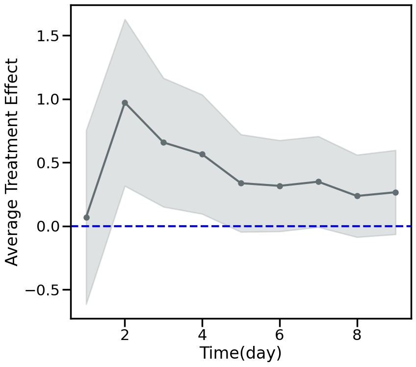
Figure 1: Change of the average treatment effect over time.

Note: The solid grey line represents the estimated effects with Difference-in-Means estimator from day 1 to day 9 for the empirical experiment, while the shaded region indicates the 95% confidence interval. The horizontal dashed blue line at 0.0 denotes the null effect baseline.

4 Identifying Sample Representativeness

Our framework first aims to assess the sample’s representativeness over time and to correct for any bias between the sample and the broader population. We begin by analyzing the sampling process throughout the experimental duration.

4.1 Stages Identification

Consider an online randomized experiment involving a population of $N$ units (e.g., users). For each unit $i$, researchers observe pre-treatment covariates $\bm{X}_{i}\in\mathcal{X}$, which may include user demographics, historical behaviors, or other baseline characteristics. The experiment assigns units to one of two conditions: treatment ($W_{i}=1$) or control ($W_{i}=0$), where $W_{i}$ denotes the binary treatment indicator. Let $Y$ represent the outcome metric of interest, and $Y_{i}(W_{i}=w)$ (or $Y_{i}(w)$ for brevity) denote the potential outcome for unit $i$ under treatment $w$. The primary estimand of interest is the population average treatment effect (PATE):

$$\tau=\mathbb{E}\left[Y_{i}(1)-Y_{i}(0)\right],$$ (1)

The above estimand cannot be directly calculated because, in practice, we only observe a sample of the population. Consequently, the causal effect must be inferred from a sample—a subset of the population that actually participated the experiment. In this paper, we focus exclusively on the nested trial design (Dahabreh and Hernán 2019), which selects random samples from the target population.

As we discussed, ongoing sampling makes it challenging to determine whether the current sample impartially represents the overall population throughout the experiment. For example, in a running experiment, users recruited in the initial days may disproportionately represent heavy users and may not accurately reflect WeChat’s full user base. Additionally, the treatment is likely to be more effective for active users, whose “previous-week” behaviors are more readily available. This uncertainty in sample composition can potentially lead to fluctuating estimations over time.

For the following discussion, let $t$ denote a specific time point within a discrete time horizon starting from zero to infinity, and $S_{it}$ denote an indicator determining whether unit $i$ is included in the experiment until time point $t$, with 1 indicating participation and 0 indicating non-participation. The sample average treatment effect (SATE) at each time point $t$ focuses on the estimate in the specific sample where units participate in:

$$\tau_{t}=\mathbb{E}[Y_{i}(1)-Y_{i}(0)|S_{it}=1].$$ (2)

The difference between $\tau$ and $\tau_{t}$ implies the bias in estimating the true effect on the target population using a limited sample, though it tends to diminish as more potential units become part of the experiment over time. We can track the progress of the sampling process by observing $Pr[S_{it}=1]$, as a higher probability of inclusion for various units suggests a more representative sample. Theoretically, the bias is going to be eliminated when all units are included in the sample as time goes to infinity, which can be expressed as $\lim\limits_{t\to\infty}Pr[S_{it}=1]=1$. Assuming that the outcome variable $Y$ is constant for a fixed unit $i$ and treatment $W_{i}=w$, the sample average treatment effect will eventually converge to an unbiased estimation of the target population average treatment effect:

$$\lim_{t\to\infty}\tau_{t} =\lim_{t\to\infty}\mathbb{E}[Y_{i}(1)-Y_{i}(0)|S_{it}=1]$$

$$=\lim_{t\to\infty}\bigg{\{}\mathbb{E}[Y_{i}(1)-Y_{i}(0)|S_{it}=1]\cdot Pr[S_{it}=1]+\mathbb{E}[Y_{i}(1)-Y_{i}(0)|S_{it}=0]\cdot Pr[S_{it}=0]\bigg{\}}$$

$$=\tau$$

In practice, the experiment can only be conducted within a finite time horizon. Thus $\tau_{t}$ will always have a margin of error on a limited time scale. Nevertheless, it’s possible to manage the estimation error within a constant bound. We define a specific tolerance level, denoted as $\rho$, whose value is positive and close to 0. As long as the bias between $\tau_{t}$ and $\tau$ shrinks to $\rho$, the sample is considered to be representative of the target population.

Definition 4.1 (Time of Representativeness)

For some constant $\rho$, there exists a time point $T_{r}$, such that the absolute difference between the sample average treatment effect and the target population average treatment effect at the period after $T_{r}$ is smaller than $\rho$, i.e.,

$$|\tau_{t}-\tau|<\rho,\ \forall\ t>T_{r}$$

The time point $T_{r}$ indicates when the sample becomes representative—meaning that unbiased estimates from the sample can be applied to the target population. In other words, $T_{r}$ marks the minimum duration after which the SATE approximately converges to the PATE. Notably, choosing a lower value for $\rho$ imposes a more stringent threshold for the permissible bias between $\tau_{t}$ and $\tau$, and vice versa.

For experiments lasting less than $T_{r}$, extrapolation-based methods can be employed to correct the sample selection bias that leads to unrepresentative samples. The key idea behind these methods is to address discrepancies between the users participating in the experiment and the target population, which arise from distribution shifts in the sample covariates over time (Degtiar and Rose 2023). Such methods typically require that the covariate distributions of the participating units do not deviate substantially from those of the target population (Imbens and Rubin 2015).

Moreover, the probability of participating in the experiment varies with different pre-treatment covariates. In the early stages of the experiment, certain regions of the covariate space may be underrepresented—for instance, users with lower activity levels might join the experiment later. This issue tends to be mitigated as the experiment’s duration increases. Referring to the definition of strict overlap (D’Amour et al. 2021), we identify a specific time point at which the overlap between the sample and the population in terms of covariate distributions is sufficiently high, thereby justifying the use of extrapolation-based methods to correct for selection bias.

Definition 4.2 (Time of Overlap)

For some constant $\eta_{o}$, there exists a time point $T_{o}$ such that for all the time period after $T_{o}$, the probability of participating in the experiment given the pre-treatment covariates exceeds $\eta_{o}$, i.e.

$$Pr[S_{it}=1|\bm{X}_{i}=\bm{x}]>\eta_{o},\ \forall\ t>T_{o}$$

Similar to the tolerance level $\rho$ defined earlier, $\eta_{o}$ is a parameter that regulates the level of overlap. The expression on the left-hand side, which represents the probability that units with given pre-treatment covariates are included in the experiment at or before time $t$, is a crucial factor in developing the generalizing framework. Let $\pi(t|\bm{X}_{i})=Pr[S_{it}=1|\bm{X}_{i}]$. We will demonstrate in the following section that $\pi(t\mid\bm{X}_{i})$ serves as an important indicator that can be modeled using lifetime distribution functions from survival analysis (Klein et al. 2003). With the aid of this model, $T_{o}$ can be identified in conjunction with the parameter $\eta_{o}$, thereby establishing a boundary for the validity of the adjusted estimation of the PATE.

In summary, we find that the time horizon and the sampling process in the experiment are naturally divided into three stages by the two time points defined above. Before $T_{o}$, no valid estimation of the PATE can be obtained from the sampled units, and and continuing the experiments is recommended. Between $T_{o}$ and $T_{r}$, estimation can be achieved through appropriate extrapolation methods, although the precision and robustness of the estimates depend heavily on the chosen model. Beyond $T_{r}$, the sampled units are representative of the target population, and the estimators for the SATE can be considered reliable and robust to the PATE. See Figure 2 for an illustration of these three stages.

Figure 2: An illustrator of the different stages divided by criteria defined by specific time points.

Note: The timeline of the experiment (along with the sampling process) is delineated into three stages: unstable stage, overlapping stage, and representative stage, by time points $T_{o}$ and $T_{r}$.

4.2 Identification Assumptions

In this section, we discuss the three key assumptions required to identify the PATE at different stages of an experiment. The first assumption safeguards the internal validity of the experiment, while the other two ensure the generalizability of the experimental results.

[Strong ignorablility] For any unit $i$ that participated in the experiment at time period $t$, given the pre-treatment covariates, the treatment assignment is conditionally independent of the potential outcome, and the conditional probability of being assigned to either treatment should be positive, i.e.

$$(Y_{i}(1),Y_{i}(0))\perp\!\!\!\perp W_{i}|\bm{X}_{i},S_{it}=1\quad and\quad Pr[W_{i}=w|\bm{X}_{i}=\bm{x},S_{it}=1]>0$$

Assumption 4.2 is derived from the condition of strongly ignorable treatment assignment introduced by Rosenbaum and Rubin (1983), which indicates the validity of causal inference drawn from the study’s results. In the context of randomized experiments, this assumption is naturally satisfied since sampled units are completely randomly assigned to different treatments.

[Conditional Exchangeability] For any unit $i$ at time $t$, participation in the experiment is conditionally independent of the potential outcome given the pre-treatment covariates:

$$Y_{i}\perp\!\!\!\perp S_{it}\mid\bm{X}_{i}.$$

Similar to the unconfoundedness condition in Rubin’s causal model (Rubin 1974), Assumption 4.2 ensures that, for fixed covariate values, the distribution of the potential outcomes is consistent between the selected sample and the target population. Equivalently, non-participation (or missing data on outcomes for non-participants) is “missing at random” (Little and Rubin 2019). The assumption implies that the probability of an outcome being missing depends only on the observed covariates and the treatment assignment does not affect the sampling process. This assumption partially ensures the possibility of inferring the PATE from sampled data using appropriate estimators.

[Positivity of Participation] For every unit $i$ and for all values of the pre-treatment covariates $\bm{X}_{i}$, the probability of participating in the experiment at time $t$ is strictly positive:

$$\Pr[S_{it}=1\mid\bm{X}_{i}=\bm{x}]>0.$$

Assumption 4.2 guarantees that the participated units overlap all sets of conditions within observable covariates. This sufficient overlap allows us to reliably infer the treatment effect for a specific group, stratified by covariates, using the results from the same group within the selected samples. Notably, when $t>T_{o}$, the positivity condition is automatically satisfied, ensuring that every subgroup defined by the observable covariates is represented in the sample. Assumption 4.2 and Assumption 4.2 collectively ensure that the experimental findings can be generalized to the target population.

4.3 Estimation Methods

We present two methods for estimating the PATE based on experimental results at different stages. It is important to note that for the period before $T_{o}$, neither method is expected to yield reliable estimates. For the period after $T_{r}$, the first method is typically employed, as it readily provides an unbiased estimation. Although the second method can also be applied after $T_{r}$, it is generally reserved for the period between $T_{o}$ and $T_{r}$ to reduce potential errors resulting from the incomplete inclusion of covariate variables.

4.3.1 Difference-in-Means Estimator

The Difference-in-Means estimator, introduced by (Splawa-Neyman et al. 1990) as an unbiased estimator for the SATE, is widely used in practical applications. In our settings, for any time $t>T_{r}$, this estimator is deemed suitable for estimating the average treatment effect on the target population.

$$\widehat{\tau}_{DIM}(t)=\frac{1}{\sum_{i=1}^{N}\text{1}\{S_{it}=1,W_{i}=1\}}\sum_{i=1}^{N}\text{1}\{S_{it}=1,W_{i}=1\}Y_{i}(1)\\ -\frac{1}{\sum_{i=1}^{N}\text{1}\{S_{it}=1,W_{i}=0\}}\sum_{i=1}^{N}\text{1}\{S_{it}=1,W_{i}=0\}Y_{i}(0).$$ (3)

4.3.2 Inverse Probability Weighting (IPW) Estimator

Derived from the Horvitz–Thompson estimator (Horvitz and Thompson 1952), the basic idea of a weighting-based estimator is to account for the distribution shift of outcomes between the sample and the target population by appropriately weighting the observations. This approach ensures that the weighted dataset is representative of the population. For instance, Stuart et al. (2011) introduced a propensity-score-based method to model the discrepancy between the sample and the target population, while Dahabreh et al. (2019) proposed an inverse probability weighting (IPW) estimator that incorporates both the probability of participation and the treatment assignment. Drawing from these methods, we define the following IPW estimator tailored to the ongoing sampling process.

$$\widehat{\tau}_{IPW}(t)=\frac{1}{\sum_{i=1}^{N}\text{1}\{S_{it}=1,W_{i}=1\}}\sum_{i=1}^{N}\frac{\text{1}\{S_{it}=1,W_{i}=1\}}{\hat{\pi}(t|\bm{X}_{i})}Y_{i}(1)\\ -\frac{1}{\sum_{i=1}^{N}\text{1}\{S_{it}=1,W_{i}=0\}}\sum_{i=1}^{N}\frac{\text{1}\{S_{it}=1,W_{i}=0\}}{\hat{\pi}(t|\bm{X}_{i})}Y_{i}(0).$$ (4)

where $\hat{\pi}(t|\bm{X}_{i})$ is an estimator for $\pi(t|\bm{X}_{i})$.

Apart from the reweighting method, alternative approaches—such as the outcome regression method and the doubly robust method—can also be employed to generate adjusted estimators (Ding and Li 2018). Although these methods are less frequently used in practice, we provide an overview of them and primarily focus on IPW estimation (see Appendix 10.2).

4.3.3 Inference

Inference for the Difference-in-Means estimator is typically performed using a two-sample t-test. In contrast, for the IPW estimator, the variance can be estimated using the sandwich estimator, which leverages meta-level statistics (Freedman 2006). However, to avoid the potentially conservative variance estimates that may arise with the sandwich estimator, the bootstrap approach is often preferred in practice (Efron and Tibshirani 1994). In our empirical studies, we demonstrate the use of the bootstrap method for inference.

5 Heuristic Method

Thus far, we have described the three stages of the ongoing sampling process in randomized experiments and the corresponding estimation strategies for each period. In the following section, we first introduce the specific survival analysis function used to model $\pi(t\mid\bm{X}_{i})$, from which the IPW estimator is naturally derived. We then demonstrate how to use $\hat{\pi}(t\mid\bm{X}_{i})$ to empirically determine the time points $T_{o}$ and $T_{r}$.

5.1 Survival Analysis

Survival analysis examines the duration of time until a specific event occurs under varying conditions (Jenkins 2005). In biomedical research, for example, the event of interest is often “death,” and researchers study factors that influence a patient’s survival time. In our context, the event of interest is “participation,” indicating that a user has been exposed to the experiment. Here, we focus on the probability that a user remains unexposed to the experiment—i.e., “survives”—beyond time $t$. Let $T$ be a random variable representing the time until participation. We can then define the survival function $S(t\mid\bm{X})$ and the lifetime distribution function $F(t\mid\bm{X})$ as follows.

$$S(t\mid\bm{X})=\Pr(T\geq t\mid\bm{X}),\qquad F(t\mid\bm{X})=1-S(t\mid\bm{X})=\Pr(T<t\mid\bm{X}).$$

Consider $T_{i}$ as the value of $T$ for a specific unit $i$. Notice that the indicator $S_{it}$ can be written as $S_{it}=\mathbf{1}\{T_{i}<t\}.$ Thus, we deduce that $\pi(t\mid\bm{X}_{i})$ is simply the realization of the lifetime distribution function for a unit with covariate profile $\bm{X}_{i}$:

$$\pi(t\mid\bm{X}_{i})=\Pr\big{(}\mathbf{1}\{T_{i}<t\}=1\mid\bm{X}_{i}\big{)}=F(t\mid\bm{X}_{i}).$$

Therefore, we can employ statistical approaches from survival analysis to model $\pi(t\mid\bm{X}_{i})$. In what follows, we introduce two methods for estimating $\pi(t\mid\bm{X}_{i})$ using the lifetime distribution function: one non-parametric method and one semi-parametric method.

5.1.1 Kaplan-Meier Estimator

The Kaplan–Meier estimator is a non-parametric method used to estimate the survival function. The resulting Kaplan–Meier survival model is a step function that decreases monotonically over time. Let $0\leq t_{1}<t_{2}<\cdots<t_{j}<\cdots$ denote the discretized time points. Given a covariate profile $\bm{X}_{i}$, we define the Kaplan–Meier estimator of the survival function as follows:

$$\hat{S}(t|\bm{X}_{i}=\bm{x})=\prod_{j:t_{j}\in[0,t]}\left(1-\frac{\sum_{i=1}^{N}\text{1}\{S_{it_{j}}=1,\bm{X}_{i}=\bm{x}\}-\sum_{i=1}^{N}\text{1}\{S_{it_{j-1}}=1,\bm{X}_{i}=\bm{x}\}}{N-\sum_{i=1}^{N}\text{1}\{S_{it_{j}}=1,\bm{X}_{i}=\bm{x}\}}\right).$$

With the Kaplan-Meier estimator, we can obtain $\hat{\pi}(t|\bm{X}_{i})$ with the plug-in approach:

$$\hat{\pi}_{KM}(t|\bm{X}_{i}=\bm{x})=\hat{F}(t|\bm{X}_{i}=\bm{x})$$

$$= 1-\prod_{j:t_{j}\in[0,t]}\left(1-\frac{\sum_{i=1}^{N}\text{1}\{S_{it_{j}}=1,\bm{X}_{i}=\bm{x}\}-\sum_{i=1}^{N}\text{1}\{S_{it_{j-1}}=1,\bm{X}_{i}=\bm{x}\}}{N-\sum_{i=1}^{N}\text{1}\{S_{it_{j}}=1,\bm{X}_{i}=\bm{x}\}}\right).$$

5.1.2 Cox Proportional Hazards Model

The Cox Proportional Hazards model is a widely used semiparametric survival model, typically employed to estimate the relative hazard—the change in the instantaneous rate of events between groups defined by distinct covariate levels. In our application, we primarily utilize the survival function obtained from a fitted Cox model, from which we derive the estimate of $\pi(t\mid\bm{X}_{i})$:

$$\hat{\pi}_{CPH}(t\mid\bm{X}_{i})=1-\hat{S}_{0}(t)^{\exp(\bm{\hat{\beta}}\cdot\bm{X}_{i})},$$

where $\hat{S}_{0}(t)$ denotes the baseline survival function corresponding to the covariate vector $\bm{X}=\bm{0}$, and $\bm{\hat{\beta}}$ is the estimated coefficient vector.

The Cox model is one of the most widely used survival models, particularly in clinical research. However, it relies on the critical assumption that the relative hazard remains constant over time across different levels of the covariates (Kuitunen et al. 2021). When this proportional hazards assumption is violated, alternative strategies can be employed. For example, one may stratify the analysis based on the covariates that do not satisfy the assumption or use an extended Cox model (Lin and Zelterman 2002).

5.2 Determination Strategies

In the subsequent sections, we will illustrate the relationship between $\hat{\pi}(t\mid\bm{X}_{i})$ and the criteria used to differentiate the sampling stages, and we will provide heuristic strategies for determining $T_{o}$ and $T_{r}$ in practice.

5.2.1 Time of Overlap

Given the definition, $T_{o}$ should be the time point where $\hat{\pi}(t\mid\bm{X}_{i}=\bm{x})>\eta_{o}$ for all $t>T_{o}$ and for every possible covariate vector in $\mathbb{X}$. Alternatively, we define

$$\hat{\pi}^{inf}(t)=\inf_{\bm{x}\in\mathbb{X}}\hat{\pi}(t\mid\bm{X}_{i}=\bm{x}),$$

which transforms the determination of $T_{o}$ into the task of finding the smallest $t$ such that $\hat{\pi}^{inf}(t)>\eta_{o}$. This ensures that even the covariate group with the lowest participation probability is adequately covered.

In practical applications, a naive approach to determining $\eta_{o}$ is to set $\eta_{o}=0.5$, meaning that for every group characterized by $\bm{X}$, the probability of participation exceeds the probability of nonparticipation. A larger value of $\eta_{o}$ provides a stronger guarantee of overlap and yields more robust estimation results; however, it also requires a longer waiting period. We consider $\hat{\pi}^{inf}(t)$ as a heuristic function for distinguishing the sampling stages. To streamline the process, we compute $\hat{\pi}^{inf}(t)$ at each time $t$ rather than aggregating the estimated participation probabilities across different values of $\bm{X}$. We then continue to use $\hat{\pi}^{inf}(t)$ to guide the determination of $T_{r}$ through its definition.

5.2.2 Time of Representativeness

When considering the periods beyond $T_{o}$, since $\widehat{\tau}_{DIM}(t)$ and $\widehat{\tau}_{IPW}(t)$ are unbiased estimators for $\tau_{t}$ and $\tau$ respectively, the upper bound of the absolute difference between these two estimands can be directly calculated. We revisit the definition of time of representativeness and develop the following proposition.

Proposition 5.1 (Upper Bound of Bias)

Consider completely randomized experiments across heterogeneous groups characterized by $\bm{X}$, for all $t>T_{o}$, the estimated absolute difference between $\tau_{t}$ and $\tau$ is less than the product of $\hat{\pi}_{inf}(t)$ and the weighted average of the absolute values of heterogeneous treatment effect, i.e.

$$|\widehat{\tau}_{DIM}(t)-\widehat{\tau}_{IPW}(t)|\leq 2\cdot\left(\frac{1}{\hat{\pi}_{inf}(t)}-1\right)\cdot\sum_{\bm{x}\in\mathbb{X}}\frac{\sum_{i=1}^{N}\text{1}\{S_{it_{j}}=1,\bm{X}_{i}=\bm{x}\}}{\sum_{i=1}^{N}\text{1}\{S_{it_{j}}=1\}}|\hat{\tau}_{HTE}(t,\bm{x})|,\ \forall\ t>T_{o}$$

where

$$\hat{\tau}_{HTE}(t,\bm{x})=\frac{1}{\sum_{i=1}^{N}\text{1}\{S_{it}=1,\bm{X}_{i}=\bm{x},W_{i}=1\}}\sum_{i=1}^{N}\text{1}\{S_{it}=1,\bm{X}_{i}=\bm{x},W_{i}=1\}Y_{i}(1)\\ -\frac{1}{\sum_{i=1}^{N}\text{1}\{S_{it}=1,\bm{X}_{i}=\bm{x},W_{i}=0\}}\sum_{i=1}^{N}\text{1}\{S_{it}=1,\bm{X}_{i}=\bm{x},W_{i}=0\}Y_{i}(0).$$

Moreover, if we assume that the weighted average of the sum of $|\hat{\tau}_{HTE}(t,\bm{x})|$ is bounded by $\frac{C}{2}\cdot|\widehat{\tau}_{DIM}(t)|$ where $C$ is a positive constant, then $T_{r}$ can be identified as the smallest $t$ that satisfies

$$\hat{\pi}^{inf}(t)>\frac{C\cdot|\widehat{\tau}_{DIM}(t)|}{\rho+C\cdot|\widehat{\tau}_{DIM}(t)|}$$

The proof of Proposition 5.1 is provided in Appendix 9.1. Intuitively, since $\widehat{\tau}_{DIM}(t)$ is equivalent to the weighted average of the heterogeneous treatment effects $\hat{\tau}_{HTE}(t,\bm{x})$, the constant $C$ will exceed two only if there exist heterogeneous groups with treatment effects in the opposite direction to the overall sample average treatment effect. This phenomenon often occurs when a treatment has an extremely pronounced negative impact on a minority group, warranting extra caution. For example, treatments tailored to appeal to a specific subset of users may be attractive to that group but may irritate the majority. Such treatments may show negligible or even negative effects on the overall population, while experiments with biased samples might fail to detect this. We have observed that the multiplier $C$ typically does not exceed two as the sample approaches representativeness (see Appendix 9.2). In practice, $C$ is often predetermined based on prior knowledge from historical experiments.

Based on Proposition 5.1, we are able to associate $T_{r}$ with the heuristic function $\hat{\pi}_{inf}(t)$ and consequently determine it. Let

$$\eta_{r}=\frac{C\cdot\sup\limits_{t\to\infty}\left\{|\widehat{\tau}_{DIM}(t)|\right\}}{\rho+C\cdot\sup\limits_{t\to\infty}\left\{|\widehat{\tau}_{DIM}(t)|\right\}},$$ (5)

the problem of determining $T_{r}$ is reframed as finding the smallest $t$ for which $\hat{\pi}^{inf}(t)$ exceeds a certain constant $\eta_{r}$.

Determining $\eta_{r}$ empirically involves a tradeoff similar to that encountered in determining $\eta_{o}$, specifically balancing experiment time against the credibility of the estimator. By eliminating the influence of the magnitude of the treatment effect across different experiments, we can express $\eta_{r}$ as:

$$\eta_{r}=\frac{C}{\frac{\rho}{\sup\limits_{t\to\infty}\left\{|\widehat{\tau}_{DIM}(t)|\right\}}+C}.$$

Considering the allowable bias $\rho$ as a proportion of $\sup\limits_{t\to\infty}\left\{|\widehat{\tau}_{DIM}(t)|\right\}$, we observe that $\eta_{r}$ is a probability value less than one. It is larger given a stricter threshold (smaller $\rho$), indicating that a longer duration of the experiment is required to achieve a more rigorous representative sample, and vice versa. Alternatively, $\eta_{r}$ can be interpreted as a parameter to control the possible bias for experiments terminated at time after $T_{r}$. Based on the above equation, the absolute difference between $\tau_{t}$ and $\tau$ is bounded by:

$$|\tau_{t}-\tau|<\rho=\frac{1-\eta_{r}}{\eta_{r}}\cdot C\cdot\sup\limits_{t\to\infty}\left\{|\widehat{\tau}_{DIM}(t)|\right\}$$

Once $\eta_{r}$ is determined, one would expect the observed difference-in-means to change by no more than $\frac{1-\eta_{r}}{\eta_{r}}\cdot C$ of the absolute value of the observed difference-in-means at time after $T_{r}$.

6 Experiments and Results

In this section, we present the results of our proposed framework at three levels: first, for the running example experiment — a specific real-world online experiment conducted on WeChat; second, for a synthetic experiment; and finally, for a platform application that scales our approach to 600 A/B tests on WeChat.

6.1 A Real-World Experiment

Before formally applying our methodology, we illustrate the sample distribution shift phenomenon in the running example by dividing the population into eight subgroups based on a key feature, labeled from level 0 to level 7. Each subgroup represents users with a specific level of this feature. We observe that higher subgroup levels correspond to users with heavier content consumption. Intuitively, the performance of the recommendation algorithm tested in this experiment is likely influenced by users’ content consumption levels, as these levels directly affect the accumulation of historical behavior records used to generate accurate recommendations.

Figure 3 presents a heat map that illustrates changes in the subgroup distribution over the experimental period. We observe that the proportion of users with high content consumption (levels 5–7) gradually decreases over time, while the proportion of dormant users increases. Given that heavy and light users may experience different treatment effects, the overall sample average treatment effect can fluctuate over time. In this experiment, the treatment involves an algorithm that ranks search results by prioritizing content consumed in the previous week. This treatment tends to affect heavy users more, as their richer historical behavior provides more data for the algorithm. Combined with the overrepresentation of heavy users in the early stages of the experiment, this partially explains why the treatment effect is particularly large during the first few days (see Figure 1). Overall, this example highlights that external validity issues caused by the ongoing sampling process of online experiments can arise from a combination of shifting covariate distributions over time and heterogeneous effects across subgroups.

Figure 3: Changes in the covariate distribution within the sample over the course of 9 days.

Note: The x-axis denotes the time in days, while the y-axis categorizes the selected sample in experiment into 8 subgroups based on the content consumption levels from 0 to 7. The color intensity, ranging from light blue to dark blue, indicates the proportion of the subgroup users in sample, with darker shades representing higher percentages.

Next, we apply our phased debiasing framework throughout the experimental period to adjust the estimation. We begin by identifying key covariates to characterize experimental units (i.e., users). Based on domain knowledge, we select variables associated with both user participation status and click-through rate, such as average login days per week, average query frequency per day, and user demographics (e.g., gender, age, and education level), as covariates in our framework. Experimenters set thresholds based on their business knowledge, tolerance for bias and preliminary calculations. $\eta_{o}$ is set to $0.5$, indicating a higher probability of participation against nonparticipation after the overlapping stage; $\eta_{r}$ is set to $0.85$, which is determined according to equation (5), where the constant $C=1.2$ precalculated from historical experiments, and $\rho=0.2\cdot\sup\limits_{t\to\infty}\left\{|\widehat{\tau}_{DIM}(t)|\right\}$ reflects a tolerance for a 20% relative estimation error in the experiments. (see Section 5.2 for details).

The heuristic function $\hat{\pi}^{inf}(t)$ is derived from a Kaplan–Meier model based on the covariates discussed in the previous sections. At each time point $t$, $\hat{\pi}^{inf}(t)$ is calculated and compared against the thresholds $\eta_{o}$ and $\eta_{r}$ to determine the current stage of the experiment. During the overlapping stage, the IPW estimator is used to adjust for bias, while the Difference-in-Means estimator continues to be applied during the representative stage.

Figure 4 presents the debiased estimation of the ATE across different experimental stages. The period prior to the overlapping stage produces unreliable estimates, as illustrated in Section 5; therefore, estimates from this phase should not be used to infer the PATE or to guide product decision-making. In other words, experimenters should refrain from stopping experiments during the unstable stage. Our debiasing framework is applied only to the later two stages: the overlapping stage and the representativeness stage. The figure demonstrates that our method enables the experiment to reveal the final, stabilized outcome (i.e., no significant treatment effect) at the beginning of the overlapping stage—2 days earlier than the unadjusted estimation (as shown in Figure 1). This indicates that product decisions can be reliably based on experiments that are stopped during either the overlapping or the representativeness stage. Identifying the specific stage of the experiment thus provides valuable guidance for experimenters, helping them assess sample representativeness and make informed decisions regarding experiment duration.

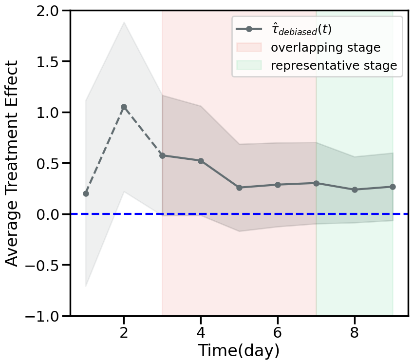
Figure 4: Debiased estimation of the average treatment effect at different experiment stages.

Note: The solid grey line represents the debiased estimated effects, with shadows indicating 95% confidence intervals. The red and green shaded regions correspond to the overlapping and representative stages of the experiment, respectively. The horizontal dashed blue line at 0.0 represents the null effect baseline.

6.2 A Synthetic Experiment

We conduct a synthetic experiment using accessible individual-level data, as real-world experiments are limited to aggregate-level data exposure due to data privacy concerns. We simulate an experiment comprising 2000 units for 30-day time period. Each unit is endowed with a covariate variable $X$, which is assigned a random value with equal probability from a sequence of increasing integers started from zero: $\{0,1,2,3\}$. The likelihood of units engaging with the product and being recruited to the experiment at time $t$ is influenced by both the active level dedicated by $X$ and the weekday/weekend effect conditional on $X$. Specifically, let $|X|$ represent the cardinality of $X$, then $\pi(t|X)$, the probability of participation in the experiment at time $t$ given $X$, derives from the following distribution :

$$\pi(t|X)=\left\{\begin{array}[]{ll}\mathcal{U}(\frac{x}{|X|},\frac{x+1}{|X|}),\ \quad\quad if\ t\ is\ on\ weekends\\ \vskip 0.05005pt\\ \mathcal{U}(\frac{x}{|X|},\frac{x+1}{|X|})/(x+1),\quad if\ t\ is\ on\ weekdays\\ \end{array}\right.$$

where $\mathcal{U}(\cdot,\cdot)$ denotes the uniform distribution.

Before any treatment is initiated, the outcome variable for all units, denoted as $Y$, follows the same normal distribution: $\mathcal{N}(1,0.01)$. We randomly assigned 1000 units to the treatment groups and the other 1000 units to the control groups, and $Y$ for each unit becomes

$$Y(x)=\left\{\begin{array}[]{ll}\mathcal{N}(0.5,0.01)+\mathcal{U}(\frac{x}{|X|},\frac{x+1}{|X|}),\quad if\ treated\\ \vskip 0.05005pt\\ \mathcal{N}(1,0.01),\quad\qquad\qquad\qquad if\ controlled\\ \end{array}\right.$$

We can easily observe that the treatment effect is more pronounced for units for the heterogenous group with a larger $X$, while the ground truth $\tau=0$ indicates no average treatment effect for the population. If we ignore the potential sample bias and directly use the difference-in-mean estimator to estimate the treatment effect, we will almost surely overestimate the true effect if we terminate the experiment in one week, as shown in Figure 7.

We attempt to model the probability of participation of units in different types, i.e. $\pi(t|X)$, through both the Kaplan-Meier model and the Cox proportional hazards model based on the synthetic data in the pre-treatment period. With the assistance of the ‘lifeline’ toolbox in Python, we can estimate and present $\hat{\pi}(t|X)$ in Figure 5.

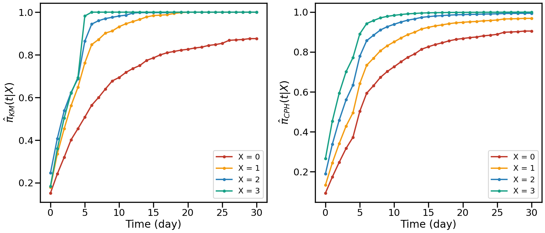
Figure 5: The estimation of $\pi(t|X)$ generated by the Kaplan-Meier model (left) and the Cox proportional hazards model (right) on the specific value of covariate $X$.

Note that here the probability of participation varies over time with different levels of $X$, leading to a violation of the proportional hazard assumption on covariate $X$ in the Cox model. Nevertheless, we observe that the Cox model exhibits to some extent robustness in this context, providing an effective estimation for $\pi(t|X)$ with differences relatively modest compared to that generated by the Kaplan-Meier model. We continue presenting results from the Cox model as a comparison approach to the Kaplan-Meier model, but we only utilize the criteria generated by the latter to determine sampling stages in the subsequent context. In practical applications, we recommend a preliminary assessment of the proportional hazards assumption on historical data before opting for the Cox model.

With the availability of $\hat{\pi}(t|X)$, the computation of the heuristic function $\hat{\pi}^{inf}(t)$ becomes straightforward, enabling the deduction of $T_{o}$ and $T_{r}$ with some pre-determined $\eta_{o}$ and $\eta_{r}$. Figure 6 illustrates an example with $\eta_{o}=0.5$ and $\eta_{r}=0.85$, showcasing $T_{o}=5$ and $T_{r}=24$ determined by $\hat{\pi}^{inf}(t)$ generated with the Kaplan-Meier model. As a comparison, the heuristic generated by the Cox model yields a similar determination for $T_{o}$ but an earlier $T_{r}$, which is $T_{r}=18$.

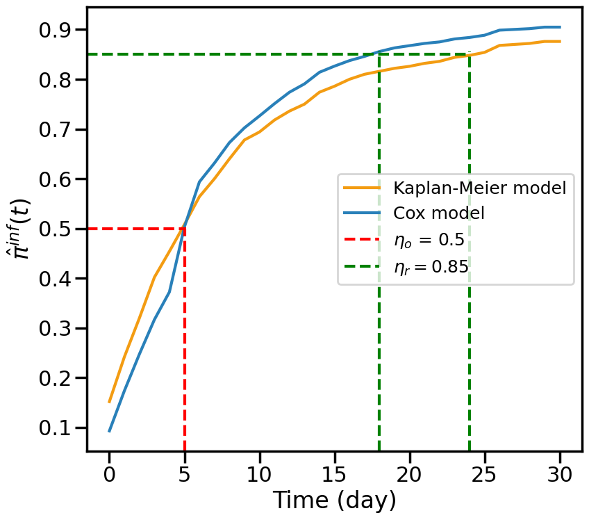
Figure 6: The heuristic function $\hat{\pi}^{inf}(t)$ over time.

Note: Blue solid curve presents the heuristic function generated with the Kaplan-Meier model, while yellow solid curve presents the heuristic function generated with the Cox proportional hazards model. Red dash line indicates the point in time when $\hat{\pi}^{inf}(t)$ reaches the threshold $\eta_{o}=0.5$, which occurs on day 5 for both models. Green dash line indicates the point in time when $\hat{\pi}^{inf}(t)$ reaches the threshold $\eta_{r}=0.85$, which is $T_{r}=18$ for the Cox model and $T_{r}=24$ for the Kaplan-Meier model.

With $T_{o}=5$ and $T_{r}=24$ determined, we proceed to apply $\hat{\pi}_{KM}(t|X)$ to generate the estimator $\hat{\tau}_{IPW}(t)$. The confidence intervals are derived from the 2.5th and 97.5th percentiles of the 1,000-times bootstrapped estimates. As a comparison, we retain the estimation results for the experiment halted before and after the overlapping stage. Figure 7 comprehensively presents the performance of the two estimators across different stages. Before $T_{o}$, $\hat{\tau}_{IPW}(t)$ exhibits extreme instability, indicating that experiments should not be halted at this stage. For experiments halted during the overlapping stage, which encompasses the time interval $T_{o}\leq t\leq T_{r}$, adjusted estimator $\hat{\tau}_{IPW}(t)$ should be adopted for effective average treatment effect estimation. For experiments halted during the representative stage occurring after $T_{r}$, $\hat{\tau}_{IPW}(t)$ performs similarly to the non-adjusted estimator $\hat{\tau}_{DIM}(t)$. Considering the convenience in the calculation, we recommend adopting $\hat{\tau}_{DIM}(t)$ as the estimation for the average treatment effect.

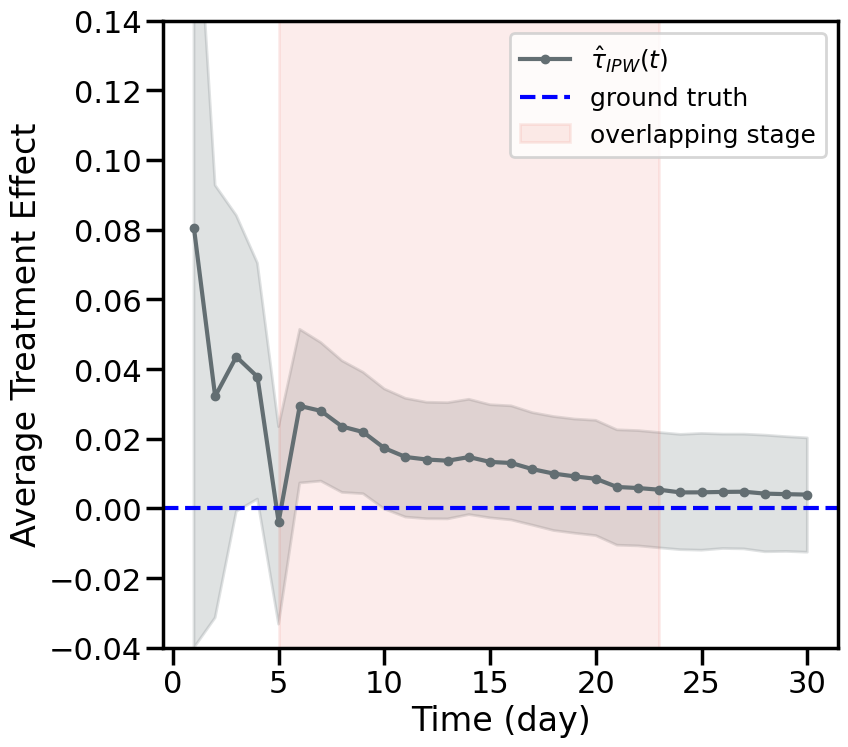
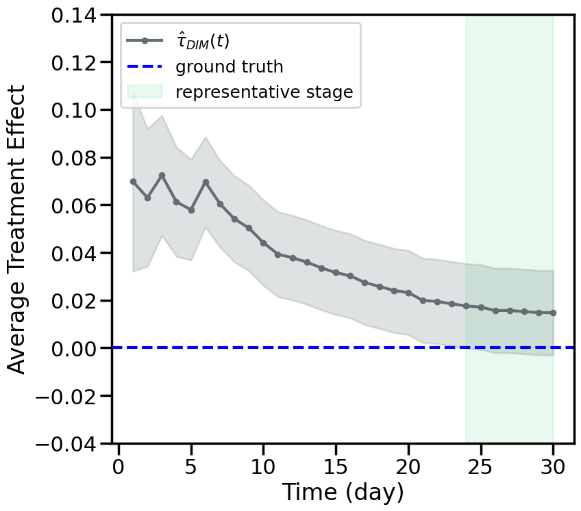
Figure 7: Treatment effect estimated by the Difference-in-Means estimator (left) and the Inverse Probability Weighting estimator (right) at different stages.

Note: Grey solid curves present the estimated effects with shadows indicating 95% confidence intervals. Blue dash line presents the true average treatment effect. The red area indicates the time interval of the overlapping stage, while the green area indicates the time interval of the representative stage.

We further assess the effectiveness of the estimators by analyzing bias and mean squared errors (MSE). For comparison, we include the Jackknife re-sampling estimator proposed by Wang et al. (2019), which, to the best of our knowledge, is the only biased-adjustment estimator that considers external validity in A/B tests. The average bias and MSE over the overlapping stage and the representative stage (time after day $5$) are presented in Table 1. The results show that the IPW estimator outperforms all methods, including the Difference-in-Means estimator (which serves as the baseline), in terms of MSE. It exhibits slightly weaker performance than the Jackknife re-sampling estimator in terms of bias. This discrepancy is attributed to the relative instability of the Jackknife re-sampling estimator in the early stages, which improves as the duration of the experiment progresses (See Figure 11 in Appendix).

In conclusion, our stage division criteria are validated, and the effectiveness of the IPW estimator constructed with the survival model is demonstrated through a synthetic experiment. We further discuss the performance of our approach in real-world experiment data.

Table 1: Comparison result between different estimators in terms of Bias and MSE for the synthetic data

Method	Bias	MSE
IPW estimator	$1.136\times 10^{-2}$	$2.637\times 10^{-4}$
Difference-in-Means estimator	$3.130\times 10^{-2}$	$1.312\times 10^{-3}$
Jackknife re-sampling estimator	$7.959\times 10^{-3}$	$3.363\times 10^{-4}$

6.3 Platform Application with 600 Experiments

To assess how our methods scale in platform operations, we applied them to 600 experiments randomly selected from the “overdone” experiments conducted across various businesses on WeChat. The selection of these experiments was based on the following criteria: 1. These experiments satisfy SUTVA, the basic assumption underlying our method. 2. The average treatment effects stabilized as the experiment duration was extended, with an average duration of over three weeks. These experiments, which happened to run for extended durations, allow us to reasonably assume that the stabilized effects observed at the end represent the true treatment effect (i.e., the “ground truth” for PATE). This offers an opportunity to evaluate our method’s ability to mitigate sampling bias and identify more effective treatments without requiring lengthy trials.

We evaluate the effectiveness of our method using two performance metrics: the False Positive Rate (FPR) and the True Positive Rate (TPR). Similar to the confusion matrix used in machine learning (Stehman 1997), we define four possible outcomes for a statistical test conducted when the experiment is terminated at a specific period. A True Positive (TP) occurs when a test correctly indicates that an effective treatment is significantly positive, whereas a True Negative (TN) occurs when a test correctly indicates that an ineffective treatment has no significant effect. Conversely, a False Positive (FP) occurs when a test incorrectly indicates that an ineffective treatment is significantly positive, and a False Negative (FN) occurs when a test incorrectly indicates that an effective treatment has no significant effect. The False Positive Rate is calculated as $FPR=\frac{FP}{FP+TN},$ which represents the probability that a non-effective treatment is mistakenly identified as having a positive effect (and potentially launched as a product). The True Positive Rate is calculated as $TPR=\frac{TP}{TP+FN},$ which represents the probability that an effective treatment is successfully detected. Our objective is to assess whether our method can increase the TPR while not increasing the FPR, thereby enhancing the overall efficacy of decision-making based on the experimental results. Based on the estimated effects at the conclusion of the experiments — the “ground truth”, we discover that out of the 600 experiments conducted, 510 reported insignificant effects, while 90 yielded significant results at a significance level of $\alpha=0.05$.

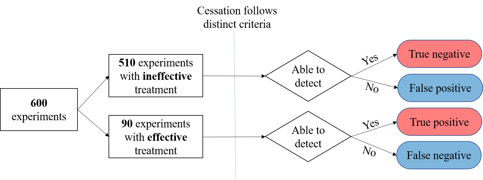
Figure 8: Illustration of categorization of empirical experiments.

We compare our framework with the commonly used baseline method for determing sample size and experiment duration based on power analysis (Deng et al. 2021, Xiang et al. 2022). Although this approach is widely adopted in practice, it does not account for external validity; instead, it guarantees that the sample size is large enough to achieve the desired power for a two-sample t-test. Specifically, at a 95% confidence level and 80% power, the minimum required sample size is given by $n=\frac{16\sigma^{2}}{\Delta^{2}},$ where $\sigma^{2}$ represents the variance of the outcome of interest, and $\Delta$ denotes the smallest treatment effect the experimenters aim to detect (Kohavi et al. 2009).

Table 2 presents a performance comparison between our method and the baseline approach, where experiment duration is determined solely by power analysis. The first column displays the results of the baseline approach, while the other three columns summarize our method’s outcomes in terms of FPR and TPR, as if the experiments had stopped at different stages. More specifically, the second column illustrates the scenario where the experiment is concluded at the overlapping stage, determined by the threshold $\eta_{o}=0.5$, with the IPW estimator employed for inference. The third and fourth columns show the experiment being terminated at the representative stage, determined by thresholds $\eta_{r}=0.8$ and $\eta_{r}=0.9$, respectively, using the Difference-in-Means estimator for statistical testing. Our framework does not recommend concluding experiments in the unstable stage.

We observe that our method consistently outperforms the baseline approach when stopping at either the overlapping or representative stages. Overall, our method increases the TPR by approximately $37$–$56\%$ while reducing the FPR by about $17$–$29\%$. This substantial improvement demonstrates that our method can identify more effective treatments without misclassifying a greater number of ineffective ones.

Table 2: Performance of Different Methods in Terms of FPR and TPR

	Baseline	Overlapping	Representative
	Approach	$(\eta_{o}=0.5)$	$(\eta_{r}=0.8)$	$(\eta_{r}=0.9)$
False Positive Rate (FPR)	11.3%	9.4%	8.8%	8.0%
True Positive Rate (TPR)	35.6%	55.6%	48.9%	48.9%

7 Practical Guidelines

In this section, we provide insights on how to apply our framework in real-world settings, including selecting covariate variables to satisfy the prerequisites and outlining the detailed procedure for implementing the approach in practical experiments.

7.1 Covariate Selection

One challenge is selecting an efficient set of covariates to satisfy both Assumption 4.2 and Assumption 4.2. In online experiments, Assumption 4.2 is typically satisfied and can be easily verified through the randomization checks, such as Sample Ratio Mismatch (SRM) test or AA test. Therefore, in the following discussion, we focus solely on the variable selection in accordance with Assumption 4.2.

To some extent, Assumption 4.2 is quite similar to the unconfoundedness assumption commonly used in observational studies, with the key distinction being that the treatment status is replaced by the indicator of participation in the experiment. In the context of unconfoundedness, we aim to control the effect of treatment assignment on the specific realization of $Y$. However, participation itself does not intrinsically affect the value of the primary outcome $Y$. Covariates can influence the estimation of treatment effects when participants and non-participants differ in their distributions and when the treatment exhibits heterogeneous effects across groups.

Figure 9 further illustrates the relationship between the sample average treatment effect $\tau$, participation $\bm{S}$, and covariate variables $\bm{X}$ over time. We can observe that the sample population is influenced by covariate variables $\bm{X}$, which control the “weight” of the treatment effect under specific covariate conditions. Simultaneously, the discrepancy between the heterogeneous treatment effect and the average treatment effect is also regulated by covariate variables. Together, these factors lead to fluctuations in the sample average treatment effect over time.

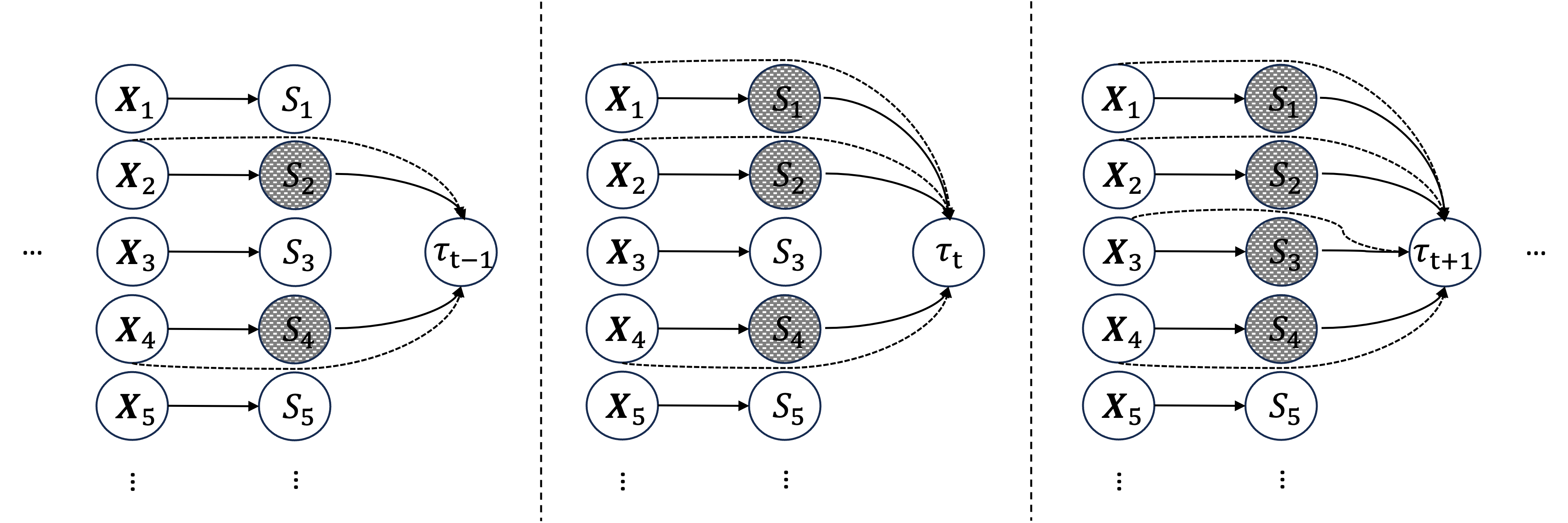
Figure 9: Illustrator of the relationship between SATE $\tau$, participation indicator $S$, and covariate variables $\bm{X}$ at different time period.

Note: Each graph separated by dash line illustrate the condition at a specific time period. Nodes highlighted in bold gray represent their presence during that time period. Solid arrows represent causal paths, indicating the sample population on which the SATE is defined at each time point. Dashed arrows imply indirect paths influencing the SATE, capturing differences in treatment effects across heterogeneous groups.

Based on the above analysis, covariates that influence both the heterogeneous treatment effect and the participation indicator $S$ should be considered to select. Furthermore, since the estimation bias - quantified by $\rho$ in Proposition 5.1 - relies on the upper bound of the sum of absolute values of the difference-in-means estimator across subgroups (a constant times the absolute value of the difference-in-means estimator), a quantitative approach is to select the (univariate) covariate $\bm{X}$ that maximizes the ratio of $|\hat{\tau}_{HTE}(t,\bm{x})|$ to $|\widehat{\tau}_{DIM}(t)|$. The higher the ratio, the greater the heterogeneity and the potential magnitude of bias. This guideline aligns with the intuition that covariates associated with both treatment effect heterogeneity and the outcome of interest are critical and should be closely monitored.

7.2 Practical Procedure

Overall, considering the generalizability of the experiment, our method provides additional information for experimenters with diverse objectives, enabling them to make optimal decisions at any stage of the experiment. From the experimenters’ perspective, we summarize the procedure of our method in Algorithm 1 as follows.

Algorithm 1 Procedure for an experiment to enhance external validity

Determine the thresholds $\eta_{o}$ and $\eta_{r}$ based on the trade-off between the generalizability of the experiment results and the experiment duration.

The experiment involves subjects whose arrival times are uncertain over an extended time horizon.

while the experiment continues at time $t$ do

  Establish the survival model in terms of whether the subject is arrived (the status of each subject) and their survival duration.

  Derive $\hat{\pi}^{inf}(t)$, compare it to $\eta_{o}$ and $\eta_{r}$ to determine the current stage of the experiment.

  if $\hat{\pi}^{inf}(t)>\eta_{o}$ then

   if Terminate the experiment then

     Estimate the treatment effect using the appropriate estimator.

     break

   end if

  end if

end while

8 Conclusion and Future Work

In this paper, we address the issue of external validity arising from covariate shifts over time in ongoing sampling processes in online experiments, such as A/B tests. To tackle this challenge, we propose a phased estimation framework aimed at improving the generalizability of experimental findings across different experiment durations. Specifically, we segment the sampling process into three stages using heuristic functions and develop tailored estimators for the average treatment effect at each stage. Our framework balances implementation cost and efficacy, as demonstrated through simulation studies, real-world experiments, and platform applications.

There are several avenues for further exploration. One direction is to investigate more sophisticated survival models for generating heuristics and developing estimators that incorporate richer covariate information. As noted, many semiparametric or parametric models in survival analysis have prerequisites, such as the proportional hazard assumption in the Cox model, which can be difficult to meet in real-world scenarios. Moreover, observational data in the IT industry tend to be high-dimensional and sparse, making it challenging to fit using traditional models without extensive feature engineering. As such, adopting deep learning models in survival analysis shows promise and warrants further exploration (Lee et al. 2018, 2019, Ranganath et al. 2016). Additionally, future research can examine external validity bias, particularly in the presence of potential unobservable factors (Andrews and Oster 2017, Nguyen et al. 2017), when the sampling dynamics cannot be fully captured by the observed covariates used in the analysis. Addressing this issue could further enhance the practical applications of our approach. Finally, the selection of thresholds $\eta_{o}$ and $\eta_{r}$ to determine the sampling stages can be further tailored to specific circumstances. We recommend developing a set of guidelines for threshold determination, informed by insights from previous experiments. A broader range of evaluation criteria could also be explored, incorporating input from various stakeholders involved in the experiment.

ONLINE APPENDICES

9 Additional Illustration of Proposition 5.1

9.1 Missing Proofs of Proposition 5.1

Proof 9.1

Proof of Proposition 5.1. From the definition of $\widehat{\tau}_{DIM}(t)$ and $\widehat{\tau}_{IPW}(t)$, we can rewrite them into following terms.

$$\widehat{\tau}_{DIM}(t) =\frac{2}{\sum_{i=1}^{N}\text{1}\{S_{it}=1\}}\left(\sum_{i=1}^{N}\text{1}\{S_{it}=1,W_{i}=1\}Y_{i}(1)-\sum_{i=1}^{N}\text{1}\{S_{it}=1,W_{i}=0\}Y_{i}(0)\right)$$

$$=\sum_{\bm{x}\in\mathbb{X}}\frac{\sum_{i=1}^{N}\text{1}\{S_{it_{j}}=1,\bm{X}_{i}=\bm{x}\}}{\sum_{i=1}^{N}\text{1}\{S_{it_{j}}=1\}}\cdot\frac{2}{\sum_{i=1}^{N}\text{1}\{S_{it_{j}}=1,\bm{X}_{i}=\bm{x}\}}\cdot$$

$$\quad\left(\sum_{i=1}^{N}\text{1}\{S_{it}=1,\bm{X}_{i}=\bm{x},W_{i}=1\}Y_{i}(1)-\sum_{i=1}^{N}\text{1}\{S_{it}=1,\bm{X}_{i}=\bm{x},W_{i}=0\}Y_{i}(0)\right)$$

$$=\sum_{\bm{x}\in\mathbb{X}}\frac{2\cdot\sum_{i=1}^{N}\text{1}\{S_{it_{j}}=1,\bm{X}_{i}=\bm{x}\}}{\sum_{i=1}^{N}\text{1}\{S_{it_{j}}=1\}}\cdot\hat{\tau}_{HTE}(t,\bm{x}).$$

$$\widehat{\tau}_{IPW}(t) =\frac{2}{\sum_{i=1}^{N}\text{1}\{S_{it}=1\}}\left(\sum_{i=1}^{N}\frac{\text{1}\{S_{it}=1,W_{i}=1\}}{\hat{\pi}(t|\bm{X}_{i})}Y_{i}(1)-\sum_{i=1}^{N}\frac{\text{1}\{S_{it}=1,W_{i}=1\}}{\hat{\pi}(t|\bm{X}_{i})}Y_{i}(0)\right)$$

$$=\sum_{\bm{x}\in\mathbb{X}}\frac{1}{\hat{\pi}(t|\bm{X}_{i}=\bm{x})}\cdot\frac{\sum_{i=1}^{N}\text{1}\{S_{it_{j}}=1,\bm{X}_{i}=\bm{x}\}}{\sum_{i=1}^{N}\text{1}\{S_{it_{j}}=1\}}\cdot\frac{2}{\sum_{i=1}^{N}\text{1}\{S_{it_{j}}=1,\bm{X}_{i}=\bm{x}\}}\cdot$$

$$\quad\left(\sum_{i=1}^{N}\text{1}\{S_{it}=1,\bm{X}_{i}=\bm{x},W_{i}=1\}Y_{i}(1)-\sum_{i=1}^{N}\text{1}\{S_{it}=1,\bm{X}_{i}=\bm{x},W_{i}=0\}Y_{i}(0)\right)$$

$$=\sum_{\bm{x}\in\mathbb{X}}\frac{2}{\hat{\pi}(t|\bm{X}_{i}=\bm{x})}\cdot\frac{\sum_{i=1}^{N}\text{1}\{S_{it_{j}}=1,\bm{X}_{i}=\bm{x}\}}{\sum_{i=1}^{N}\text{1}\{S_{it_{j}}=1\}}\cdot\hat{\tau}_{HTE}(t,\bm{x}).$$

Note that $\sum_{i=1}^{N}\text{1}\{S_{it}=1,\bm{X}_{i}=\bm{x},W_{i}=0\}=\sum_{i=1}^{N}\text{1}\{S_{it}=1,\bm{X}_{i}=\bm{x},W_{i}=1\}=\frac{1}{2}\cdot\sum_{i=1}^{N}\text{1}\{S_{it}=1,\bm{X}_{i}=\bm{x}\}$ holds by default as we assume that the intervention is completely randomly assigned across heterogenous groups defined by $\bm{X}$.

Therefore the estimated absolute difference can be written as

$$|\widehat{\tau}_{DIM}(t)-\widehat{\tau}_{IPW}(t)| =2\cdot\left|\sum_{\bm{x}\in\mathbb{X}}\left(1-\frac{1}{\hat{\pi}(t|\bm{X}_{i}=\bm{x})}\right)\frac{\sum_{i=1}^{N}\text{1}\{S_{it_{j}}=1,\bm{X}_{i}=\bm{x}\}}{\sum_{i=1}^{N}\text{1}\{S_{it_{j}}=1\}}\cdot\hat{\tau}_{HTE}(t,\bm{x})\right|$$

$$\leq 2\cdot\left(\frac{1}{\hat{\pi}_{inf}(t)}-1\right)\sum_{\bm{x}\in\mathbb{X}}\frac{\sum_{i=1}^{N}\text{1}\{S_{it_{j}}=1,\bm{X}_{i}=\bm{x}\}}{\sum_{i=1}^{N}\text{1}\{S_{it_{j}}=1\}}\cdot\left|\hat{\tau}_{HTE}(t,\bm{x})\right|.$$

Since

$$\sum_{\bm{x}\in\mathbb{X}}\frac{\sum_{i=1}^{N}\text{1}\{S_{it_{j}}=1,\bm{X}_{i}=\bm{x}\}}{\sum_{i=1}^{N}\text{1}\{S_{it_{j}}=1\}}\cdot\left|\hat{\tau}_{HTE}(t,\bm{x})\right|\leq\frac{C}{2}\cdot|\widehat{\tau}_{DIM}(t)|,$$

We can further scale the inequality as follows

$$|\widehat{\tau}_{DIM}(t)-\widehat{\tau}_{IPW}(t)|\leq C\cdot|\widehat{\tau}_{DIM}(t)|\cdot\left(\frac{1}{\hat{\pi}_{inf}(t)}-1\right)<\rho$$

By the definition of $T_{r}$, our goal is to identify a specific time $t$ at which the upper bound of the estimated absolute difference falls below the threshold $\rho$. The heuristic function $\hat{\pi}_{inf}(t)$ thus should fulfill the following condition.

$$\hat{\pi}_{inf}(t)>\frac{1}{1+\frac{\rho}{C\cdot|\widehat{\tau}_{DIM}(t)|}}>\frac{C\cdot|\widehat{\tau}_{DIM}(t)|}{\rho+C\cdot|\widehat{\tau}_{DIM}(t)|}$$

9.2 The Value of $C$

Empirically, the constant $C$ can be learned through the historical records. Figure 10 visualizes the values of the constant $C$ in 268 sampled experiments on Weixin experimentation platform. Our empirical result suggests that the value $C$ is relatively stable across the experiments, regardless the duration. Thus, choosing the empirical values of $C=2$ should be relatively robust. Note that in our sampled experiments, the outcome of is interest is some measurement of activeness and the covariates used is active level of participants, whose distribution is changing over the time and is highly correlated to the outcome of interest.

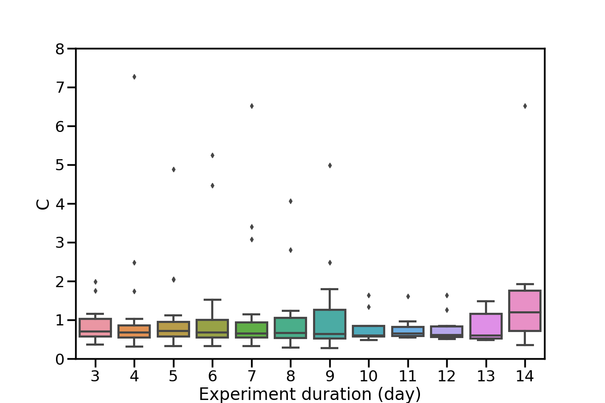
Figure 10: The boxplot of ratio constant $C$ in 268 sampled experiments.

10 Estimation Methods

10.1 IPW Estimator Unbiasedness Proof

Similar to Stuart et al. (2011), we provide evidence to show that the expectation of the IPW estimator is equal to the population average treatment effect.

Let $e_{wt}(\bm{X}_{i})=Pr\left[W_{i}=w|\bm{X}_{i},S_{it}=1\right]$ denotes the probability of treatment assignment for participated units, which is similar to the propensity score used in observational study (Rosenbaum and Rubin 1983). We assume the strong ignorability, $W_{i}\perp\!\!\!\perp\{Y_{i}(1),Y_{i}(0)\}|\bm{X}_{i}$, which is naturally satisfied in randomized controlled experiments. It is obvious that

$$\pi(t|\bm{X}_{i})\cdot e_{wt}(\bm{X}_{i})=Pr\left[S_{it}=1,W_{i}=w|\bm{X}_{i}\right]=\mathbb{E}\left\{\text{1}\{S_{it}=1,W_{i}=w\}|\bm{X}_{i}\right\}$$

Therefore, we have

$$\mathbb{E}\left\{\frac{\text{1}\{S_{it}=1,W_{i}=w\}Y_{i}}{\pi(t|\bm{X}_{i})e_{wt}(\bm{X}_{i})}\right\} =\mathbb{E}\left\{\frac{\text{1}\{S_{it}=1,W_{i}=w\}Y_{i}(w)}{\pi(t|\bm{X}_{i})e_{wt}(\bm{X}_{i})}\right\}$$

$$=\mathbb{E}\left[\mathbb{E}\left\{\frac{\text{1}\{S_{it}=1,W_{i}=w\}Y_{i}(w)}{\pi(t|\bm{X}_{i})e_{wt}(\bm{X}_{i})}\Bigg{|}\bm{X}_{i}\right\}\right]$$

$$=\mathbb{E}\left[\frac{1}{\pi(t|\bm{X}_{i})e_{wt}(\bm{X}_{i})}\mathbb{E}\left\{\text{1}\{S_{it}=1,W_{i}=w\}Y_{i}(w)|\bm{X}_{i}\right\}\right]$$

$$=\mathbb{E}\left[\frac{1}{\pi(t|\bm{X}_{i})e_{wt}(\bm{X}_{i})}\mathbb{E}\left\{\text{1}\{S_{it}=1,W_{i}=w\}|\bm{X}_{i}\right\}\mathbb{E}\left\{Y_{i}(w)|\bm{X}_{i}\right\}\right]$$

$$=\mathbb{E}\left[\mathbb{E}\left\{Y_{i}(w)|\bm{X}_{i}\right\}\right]$$

$$=\mathbb{E}\left[Y_{i}(w)\right]$$

Due to the randomized controlled setting, $e_{wt}(\bm{X}_{i})$ is pre-determined before the experiment starts. A naive estimator to $e_{wt}(\bm{X}_{i})$ is $\sum_{i=1}^{N}\text{1}\{S_{it}=1,W_{i}=w\}/N$. Since the sample mean is an unbiased estimation of expectation under the central limit theorem, the unbiasedness of the IPW estimator is evidently established.

10.2 Alternative Estimators

In addition to the IPW estimator discussed in the main context, there are other adjusted estimators commonly employed to correct covariate distribution imbalances. We propose the following estimators as practical alternatives to the IPW estimator.

10.2.1 Outcome Model-based Estimator

This approach is suggested under the premise that we can regard the outcome of units that have not participated in the experiment as ’missing data’, and fill in with proper values generated by an outcome regression model.

$$\widehat{\tau}(t)=\frac{1}{N}\sum_{i=1}^{N}(\hat{\mathbb{E}}[Y_{i}|\bm{X}_{i},S_{it}=1,W_{i}=1]-\hat{\mathbb{E}}[Y_{i}|\bm{X}_{i},S_{it}=1,W_{i}=0])$$

10.2.2 Doubly Robust Estimator

Let $\hat{g}_{wt}(\bm{X}_{i})=\hat{\mathbb{E}}[Y_{i}|\bm{X}_{i},S_{it}=1,W_{i}=w]$ be the outcome model we used to predict the ’missing’ outcomes. By integrating the reweighting approach with the outcome model-based approach, we formulate the following doubly robust estimator.

$$\widehat{\tau}(t)=\frac{1}{\sum_{i=1}^{N}\text{1}\{S_{it}=1,W_{i}=1\}}\sum_{i=1}^{N}\frac{\text{1}\{S_{it}=1,W_{i}=1\}}{\hat{\pi}(t|\bm{X}_{i})}(Y_{i}(1)-\hat{g}_{1t})\\ -\frac{1}{\sum_{i=1}^{N}\text{1}\{S_{it}=1,W_{i}=0\}}\sum_{i=1}^{N}\frac{\text{1}\{S_{it}=1,W_{i}=0\}}{\hat{\pi}(t|\bm{X}_{i})}(Y_{i}(0)-\hat{g}_{0t})+\frac{1}{N}\sum_{i=1}^{N}(g_{1t}(\bm{X}_{i})-\hat{g}_{0t}(\bm{X}_{i})).$$

10.2.3 Jackknife re-sampling estimator

Wang et al. (2019) introduced a bias-adjusted estimator based on jackknife considering the first-order heavy-user bias in A/B test. We apply this estimator as a comparison to our methods in the main context. The performance of the Jackknife re-sampling estimator in the synthetic experiment is illustrated in Figure 11.

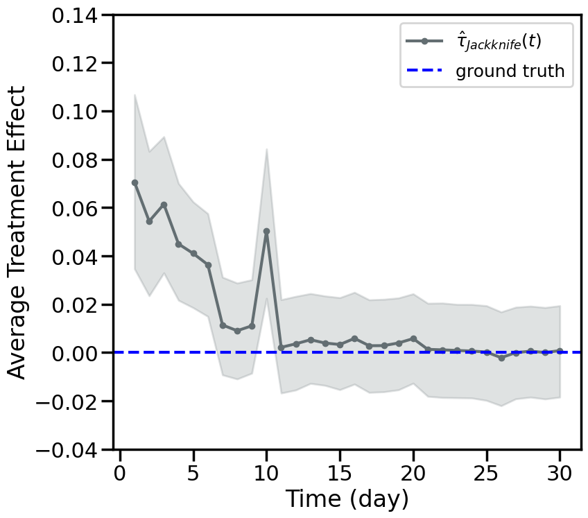
Figure 11: Treatment effect estimated by the Jackknife re-sampling estimator in the synthetic experiment

11 The Performance of the Survival Model

We assess the performance of two survival models, the Kaplan-Meier model and the Cox model, using the AUC score. Specifically, we split the entire experiment dataset into 90% for training and 10% for testing. Note that at time $t$, we can observe $t$-period experimental data which is right censored, since subjects who have not participated in the experiment are still survived, albeit with an unknown survival duration. We fit the survival model on the training data, assuming that the experiment stops at each time $t$ within 30-day periods, and compute the AUC score on the test data. The results are presented in Figure 12. The mean AUC score over time for the Kaplan-Meier model is 0.8270 (s.e. 0.009911), while the mean AUC score for the Cox model is 0.8267 (s.e. 0.009880).

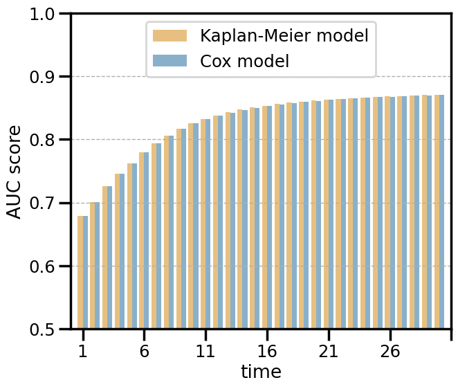
Figure 12: The AUC score of survival models at different experiment stopping times.

12 Supplement to Results

As we showcase the FPR and TPR in Table 2 to illustrate the performance of our framework in practice, here we add the original number of experiments for the four metrics (TN, FP, FN, TP) as complementary data.

Table 3: The number of experiments for each metric among 600 experiments

	the baseline	overlapping	representative	representative
	approach	($\eta=0.5$)	($\eta^{\prime}=0.8$)	($\eta^{\prime}=0.9$)
True Negative (TN)	452	462	465	469
False Positive (FP)	58	48	45	41
False Negative (FN)	58	49	46	46
True Positive (TP)	32	41	44	44

13 Internal Validity Check

Sample Ratio Mismatch (SRM) occurs when the observed number of users in each group does not align with the allocation specified by the experimenters, which is intended to be 1:1. A chi-square test is conducted to determine whether the traffic allocation meets the expected distribution. After applying the After applying the Bonferroni, Benjamini-Hochberg (BH), or Benjamini-Yekutieli (BY) to account for multiple testing(Bonferroni 1936, Hochberg and Benjamini 1990, Benjamini and Hochberg 1995), we found no evidence of SRM issues throughout the experiments, either at the significance level of $\alpha=0.05$ or $\alpha=0.01$.

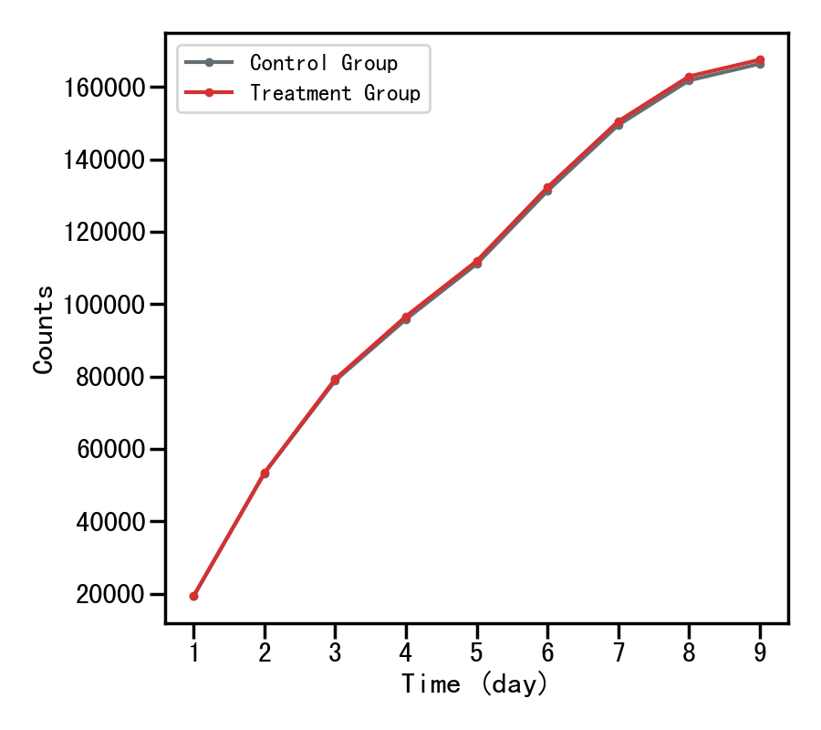
Figure 13: Cumulative sample size for treatment and control groups in the experiment

Furthermore, we sought to assess significant differences between the two groups by conducting t-tests on eight key covariates, which were anticipated to show no significant differences. Table 4 presents the results of these tests, comparing the performance of the two groups across the eight key metrics during the seven days leading up to the start of the experimentation. These eight metrics include the primary outcome of interest, one activeness metric, and six consumption metrics, selected by the experimenters based on their domain expertise. As users accumulate on a daily basis, we conducted the same tests for each day. After applying the Bonferroni, Benjamini-Hochberg (BH), or Benjamini-Yekutieli (BY) procedures to account for multiple hypothesis testing, we found that none of the key metrics exhibited statistically significant differences on any day at the $\alpha=0.05$ or $\alpha=0.01$ levels. This indicates an internally valid traffic allocation for comparable experimental groups.

Table 4: Relative differences of pre-treatment outcomes for 8 key metrics (p-values in parentheses)

Metric	Day 1	Day 2	Day 3	Day 4	Day 5	Day 6	Day 7	Day 8	Day 9
Primary	0.419% (0.45769)	0.663% (0.04822)	0.581% (0.04204)	0.493% (0.05641)	0.363% (0.13)	0.344% (0.11762)	0.323% (0.11935)	0.3% (0.13247)	0.292% (0.13908)
Activeness	1.259% (0.38484)	0.563% (0.52598)	0.557% (0.45338)	0.405% (0.55428)	0.312% (0.62634)	0.354% (0.55271)	0.223% (0.6921)	0.134% (0.80574)	0.076% (0.8888)
Consump. 1	5.033% (0.2321)	1.216% (0.57619)	2.127% (0.23415)	2.744% (0.12604)	3.083% (0.0665)	3.913% (0.01172)	3.474% (0.01778)	3.179% (0.02476)	2.951% (0.03436)
Consump. 2	2.172% (0.17794)	0.624% (0.51075)	0.648% (0.42173)	0.581% (0.44114)	0.596% (0.40142)	0.882% (0.18027)	0.744% (0.23381)	0.615% (0.30905)	0.514% (0.38927)
Consump. 3	-0.676% (0.68749)	-0.572% (0.55406)	-0.519% (0.51384)	-0.547% (0.45269)	-0.584% (0.39193)	-0.289% (0.64583)	-0.251% (0.67314)	-0.268% (0.64082)	-0.329% (0.56286)
Consump. 4	-0.761% (0.6112)	-0.286% (0.7392)	-0.312% (0.65693)	-0.34% (0.59852)	-0.475% (0.43397)	-0.34% (0.54317)	-0.369% (0.48524)	-0.418% (0.41306)	-0.468% (0.35402)
Consump. 5	-0.761% (0.6112)	-0.286% (0.7392)	-0.312% (0.65693)	-0.34% (0.59852)	-0.475% (0.43397)	-0.34% (0.54317)	-0.369% (0.48524)	-0.418% (0.41306)	-0.468% (0.35402)
Consump. 6	0.474% (0.74931)	0.36% (0.67702)	0.226% (0.75208)	0.156% (0.81267)	0.015% (0.98103)	0.217% (0.70528)	0.193% (0.72119)	0.123% (0.81438)	0.048% (0.92532)

References

- Adam et al. (2023) Adam H, Yin F, Hu M, Tenenholtz N, Crawford L, Mackey L, Koenecke A (2023) Should i stop or should i go: Early stopping with heterogeneous populations. arXiv preprint arXiv:2306.11839 .
- Andrews and Oster (2017) Andrews I, Oster E (2017) Weighting for external validity .
- Aral and Walker (2012) Aral S, Walker D (2012) Identifying influential and susceptible members of social networks. Science 337(6092):337–341.
- Bell et al. (2016) Bell SH, Olsen RB, Orr LL, Stuart EA (2016) Estimates of external validity bias when impact evaluations select sites nonrandomly. Educational evaluation and policy analysis 38(2):318–335.
- Benjamini and Hochberg (1995) Benjamini Y, Hochberg Y (1995) Controlling the false discovery rate: a practical and powerful approach to multiple testing. Journal of the Royal statistical society: series B (Methodological) 57(1):289–300.
- Bonferroni (1936) Bonferroni C (1936) Teoria statistica delle classi e calcolo delle probabilita. Pubblicazioni del R istituto superiore di scienze economiche e commericiali di firenze 8:3–62.
- Bracht and Glass (1968) Bracht GH, Glass GV (1968) The external validity of experiments. American educational research journal 5(4):437–474.
- Braslow et al. (2005) Braslow JT, Duan N, Starks SL, Polo A, Bromley E, Wells KB (2005) Generalizability of studies on mental health treatment and outcomes, 1981 to 1996. Psychiatric Services 56(10):1261–1268.
- Campbell (1986) Campbell DT (1986) Relabeling internal and external validity for applied social scientists. New Directions for Program Evaluation 1986(31):67–77.
- Clark et al. (2003) Clark TG, Bradburn MJ, Love SB, Altman DG (2003) Survival analysis part i: basic concepts and first analyses. British journal of cancer 89(2):232–238.
- Cox (1958) Cox DR (1958) Planning of experiments. .
- Dahabreh and Hernán (2019) Dahabreh IJ, Hernán MA (2019) Extending inferences from a randomized trial to a target population. European journal of epidemiology 34:719–722.
- Dahabreh et al. (2020) Dahabreh IJ, Robertson SE, Steingrimsson JA, Stuart EA, Hernan MA (2020) Extending inferences from a randomized trial to a new target population. Statistics in medicine 39(14):1999–2014.
- Dahabreh et al. (2019) Dahabreh IJ, Robertson SE, Tchetgen EJ, Stuart EA, Hernán MA (2019) Generalizing causal inferences from individuals in randomized trials to all trial-eligible individuals. Biometrics 75(2):685–694.
- De Angelis et al. (1999) De Angelis R, Capocaccia R, Hakulinen T, Soderman B, Verdecchia A (1999) Mixture models for cancer survival analysis: application to population-based data with covariates. Statistics in medicine 18(4):441–454.
- Degtiar and Rose (2023) Degtiar I, Rose S (2023) A review of generalizability and transportability. Annual Review of Statistics and Its Application 10:501–524.
- Demediuk et al. (2018) Demediuk S, Murrin A, Bulger D, Hitchens M, Drachen A, Raffe WL, Tamassia M (2018) Player retention in league of legends: a study using survival analysis. Proceedings of the Australasian computer science week multiconference, 1–9.
- Deng et al. (2021) Deng A, Li Y, Lu J, Ramamurthy V (2021) On post-selection inference in a/b testing. Proceedings of the 27th ACM SIGKDD Conference on Knowledge Discovery & Data Mining, 2743–2752.
- Deng et al. (2016) Deng A, Lu J, Chen S (2016) Continuous monitoring of a/b tests without pain: Optional stopping in bayesian testing. 2016 IEEE International conference on data science and advanced analytics (DSAA), 243–252 (IEEE).
- Ding and Li (2018) Ding P, Li F (2018) Causal inference. Statistical Science 33(2):214–237.
- D’Amour et al. (2021) D’Amour A, Ding P, Feller A, Lei L, Sekhon J (2021) Overlap in observational studies with high-dimensional covariates. Journal of Econometrics 221(2):644–654.
- Efron and Tibshirani (1994) Efron B, Tibshirani RJ (1994) An introduction to the bootstrap (CRC press).
- Egami and Hartman (2021) Egami N, Hartman E (2021) Covariate selection for generalizing experimental results: application to a large-scale development program in uganda. Journal of the Royal Statistical Society Series A: Statistics in Society 184(4):1524–1548.
- Egami and Hartman (2023) Egami N, Hartman E (2023) Elements of external validity: Framework, design, and analysis. American Political Science Review 117(3):1070–1088.
- Findley et al. (2021) Findley MG, Kikuta K, Denly M (2021) External validity. Annual Review of Political Science 24:365–393.
- Finney et al. (1950) Finney D, et al. (1950) An example of periodic variation in forest sampling. Forestry 23(2):96–111.
- Freedman (2006) Freedman DA (2006) On the so-called “huber sandwich estimator” and “robust standard errors”. The American Statistician 60(4):299–302.
- Hochberg and Benjamini (1990) Hochberg Y, Benjamini Y (1990) More powerful procedures for multiple significance testing. Statistics in medicine 9(7):811–818.
- Hohnhold et al. (2015) Hohnhold H, O’Brien D, Tang D (2015) Focusing on the long-term: It’s good for users and business. Proceedings of the 21th ACM SIGKDD International Conference on Knowledge Discovery and Data Mining, 1849–1858.
- Horvitz and Thompson (1952) Horvitz DG, Thompson DJ (1952) A generalization of sampling without replacement from a finite universe. Journal of the American statistical Association 663–685.
- Hu et al. (2021) Hu S, Chen P, Chen X (2021) Do personalized economic incentives work in promoting shared mobility? examining customer churn using a time-varying cox model. Transportation Research Part C: Emerging Technologies 128:103224.
- Huang et al. (2023) Huang S, Wang C, Yuan Y, Zhao J, Zhang J (2023) Estimating effects of long-term treatments. arXiv preprint arXiv:2308.08152 .
- Hubbard et al. (2010) Hubbard AE, Ahern J, Fleischer NL, Van der Laan M, Lippman SA, Jewell N, Bruckner T, Satariano WA (2010) To gee or not to gee: comparing population average and mixed models for estimating the associations between neighborhood risk factors and health. Epidemiology 21(4):467–474.
- Imbens and Rubin (2015) Imbens GW, Rubin DB (2015) Causal inference in statistics, social, and biomedical sciences (Cambridge University Press).
- Jenkins (2005) Jenkins SP (2005) Survival analysis. Unpublished manuscript, Institute for Social and Economic Research, University of Essex, Colchester, UK 42:54–56.
- Jeong and Namkoong (2020) Jeong S, Namkoong H (2020) Assessing external validity over worst-case subpopulations. arXiv preprint arXiv:2007.02411 .
- Johari et al. (2022) Johari R, Koomen P, Pekelis L, Walsh D (2022) Always valid inference: Continuous monitoring of a/b tests. Operations Research 70(3):1806–1821.
- Kelly and Lim (2000) Kelly PJ, Lim LLY (2000) Survival analysis for recurrent event data: an application to childhood infectious diseases. Statistics in medicine 19(1):13–33.
- Kern et al. (2016) Kern HL, Stuart EA, Hill J, Green DP (2016) Assessing methods for generalizing experimental impact estimates to target populations. Journal of research on educational effectiveness 9(1):103–127.
- Klein et al. (2003) Klein JP, Moeschberger ML, et al. (2003) Survival analysis: techniques for censored and truncated data, volume 1230 (Springer).
- Kohavi et al. (2012) Kohavi R, Deng A, Frasca B, Longbotham R, Walker T, Xu Y (2012) Trustworthy online controlled experiments: Five puzzling outcomes explained. Proceedings of the 18th ACM SIGKDD international conference on Knowledge discovery and data mining, 786–794.
- Kohavi et al. (2009) Kohavi R, Longbotham R, Sommerfield D, Henne RM (2009) Controlled experiments on the web: survey and practical guide. Data mining and knowledge discovery 18:140–181.
- Kohavi et al. (2020) Kohavi R, Tang D, Xu Y (2020) Trustworthy online controlled experiments: A practical guide to a/b testing (Cambridge University Press).
- Kuitunen et al. (2021) Kuitunen I, Ponkilainen VT, Uimonen MM, Eskelinen A, Reito A (2021) Testing the proportional hazards assumption in cox regression and dealing with possible non-proportionality in total joint arthroplasty research: methodological perspectives and review. BMC musculoskeletal disorders 22(1):489.
- Lee et al. (2019) Lee C, Yoon J, Van Der Schaar M (2019) Dynamic-deephit: A deep learning approach for dynamic survival analysis with competing risks based on longitudinal data. IEEE Transactions on Biomedical Engineering 67(1):122–133.
- Lee et al. (2018) Lee C, Zame W, Yoon J, Van Der Schaar M (2018) Deephit: A deep learning approach to survival analysis with competing risks. Proceedings of the AAAI conference on artificial intelligence, volume 32.
- Lenth (2001) Lenth RV (2001) Some practical guidelines for effective sample size determination. The American Statistician 55(3):187–193.
- Lesko et al. (2017) Lesko CR, Buchanan AL, Westreich D, Edwards JK, Hudgens MG, Cole SR (2017) Generalizing study results: a potential outcomes perspective. Epidemiology (Cambridge, Mass.) 28(4):553.
- Lin and Zelterman (2002) Lin H, Zelterman D (2002) Modeling survival data: extending the cox model.
- Little and Rubin (2019) Little RJ, Rubin DB (2019) Statistical analysis with missing data, volume 793 (John Wiley & Sons).
- Liu (2012) Liu X (2012) Survival analysis: models and applications (John Wiley & Sons).
- Machin et al. (2006) Machin D, Cheung YB, Parmar M (2006) Survival analysis: a practical approach (John Wiley & Sons).
- Maharaj et al. (2023) Maharaj A, Sinha R, Arbour D, Waudby-Smith I, Liu SZ, Sinha M, Addanki R, Ramdas A, Garg M, Swaminathan V (2023) Anytime-valid confidence sequences in an enterprise a/b testing platform. Companion Proceedings of the ACM Web Conference 2023, 396–400.
- Nguyen et al. (2017) Nguyen TQ, Ebnesajjad C, Cole SR, Stuart EA (2017) Sensitivity analysis for an unobserved moderator in rct-to-target-population generalization of treatment effects. The Annals of Applied Statistics 225–247.
- Ranganath et al. (2016) Ranganath R, Perotte A, Elhadad N, Blei D (2016) Deep survival analysis. Machine Learning for Healthcare Conference, 101–114 (PMLR).
- Rosenbaum and Rubin (1983) Rosenbaum PR, Rubin DB (1983) The central role of the propensity score in observational studies for causal effects. Biometrika 70(1):41–55.
- Rothwell (2005) Rothwell PM (2005) External validity of randomised controlled trials:“to whom do the results of this trial apply?”. The Lancet 365(9453):82–93.
- Rubin (1974) Rubin DB (1974) Estimating causal effects of treatments in randomized and nonrandomized studies. Journal of educational Psychology 66(5):688.
- Rubin (1980) Rubin DB (1980) Randomization analysis of experimental data: The fisher randomization test comment. Journal of the American statistical association 75(371):591–593.
- Schönbrodt et al. (2017) Schönbrodt FD, Wagenmakers EJ, Zehetleitner M, Perugini M (2017) Sequential hypothesis testing with bayes factors: Efficiently testing mean differences. Psychological methods 22(2):322.
- Shulman et al. (2023) Shulman JD, Toubia O, Saddler R (2023) Marketing’s role in the evolving discipline of product management. Marketing Science 42(1):1–5.
- Simester et al. (2022) Simester D, Timoshenko A, Zoumpoulis SI (2022) A sample size calculation for training and certifying targeting policies .
- Slack and Draugalis Jr (2001) Slack MK, Draugalis Jr JR (2001) Establishing the internal and external validity of experimental studies. American journal of health-system pharmacy 58(22):2173–2181.
- Splawa-Neyman et al. (1990) Splawa-Neyman J, Dabrowska DM, Speed TP (1990) On the application of probability theory to agricultural experiments. essay on principles. section 9. Statistical Science 465–472.
- Stehman (1997) Stehman SV (1997) Selecting and interpreting measures of thematic classification accuracy. Remote sensing of Environment 62(1):77–89.
- Stuart et al. (2011) Stuart EA, Cole SR, Bradshaw CP, Leaf PJ (2011) The use of propensity scores to assess the generalizability of results from randomized trials. Journal of the Royal Statistical Society Series A: Statistics in Society 174(2):369–386.
- Stuart and Rhodes (2017) Stuart EA, Rhodes A (2017) Generalizing treatment effect estimates from sample to population: A case study in the difficulties of finding sufficient data. Evaluation review 41(4):357–388.
- Susukida et al. (2016) Susukida R, Crum RM, Stuart EA, Ebnesajjad C, Mojtabai R (2016) Assessing sample representativeness in randomized controlled trials: application to the national institute of drug abuse clinical trials network. Addiction 111(7):1226–1234.
- Tipton (2013) Tipton E (2013) Improving generalizations from experiments using propensity score subclassification: Assumptions, properties, and contexts. Journal of Educational and Behavioral Statistics 38(3):239–266.
- Tipton et al. (2016) Tipton E, Fellers L, Caverly S, Vaden-Kiernan M, Borman G, Sullivan K, Ruiz de Castilla V (2016) Site selection in experiments: An assessment of site recruitment and generalizability in two scale-up studies. Journal of Research on Educational Effectiveness 9(sup1):209–228.
- Viechtbauer et al. (2015) Viechtbauer W, Smits L, Kotz D, Budé L, Spigt M, Serroyen J, Crutzen R (2015) A simple formula for the calculation of sample size in pilot studies. Journal of clinical epidemiology 68(11):1375–1379.
- Wang et al. (2019) Wang Y, Gupta S, Lu J, Mahmoudzadeh A, Liu S (2019) On heavy-user bias in a/b testing. Proceedings of the 28th ACM International Conference on Information and Knowledge Management, 2425–2428.
- Xiang et al. (2022) Xiang D, West R, Wang J, Cui X, Huang J (2022) Multi armed bandit vs. a/b tests in e-commerce-confidence interval and hypothesis test power perspectives. Proceedings of the 28th ACM SIGKDD conference on knowledge discovery and data mining, 4204–4214.