Asymptotics for first passage percolation on logarithmic subgraphs of $\mathbb{Z}^{2}$

Abstract

For $a>0$ and $b\geq 0$, let $\mathbb{G}_{a,b}$ be the subgraph of $\mathbb{Z}^{2}$ induced by the vertices between the first coordinate axis and the graph of the function $f=f_{a,b}(u)=a\log(1+u)+b\log(1+\log(1+u))$, $u\geq 0$. It is known that for $a>0$, the critical value for Bernoulli percolation on $\mathbb{G}_{f}=\mathbb{G}_{a,b}$ is strictly between $1/2$ and $1$, and that if $b>2a$ then the percolation phase transition is discontinuous. We study first-passage percolation (FPP) on $\mathbb{G}_{a,b}$ with i.i.d. edge-weights $(\tau_{e})$ satisfying $p=\mathbb{P}(\tau_{e}=0)\in[1/2,1)$ and the “gap condition” $\mathbb{P}(\tau_{e}\leq\delta)=p$ for some $\delta>0$. We find the rate of growth of the expected passage time in $\mathbb{G}_{f}$ from the origin to the line $x=n$, and show that, while when $p=1/2$ it is of order $n/(a\log n)$, when $p>1/2$ it can be of order (a) $n^{c_{1}}/(\log n)^{c_{2}}$, (b) $(\log n)^{c_{3}}$, (c) $\log\log n$, or (d) constant, depending on the relationship between $a,b,$ and $p$. For more general functions $f$, we prove a central limit theorem for the passage time and show that its variance grows at the same rate as the mean. As a consequence of our methods, we improve the percolation transition result by showing that the phase transition on $\mathbb{G}_{a,b}$ is discontinuous if and only if $b>a$, and improve “sponge crossing dimensions” asymptotics from the ’80s on subcritical percolation crossing probabilities for tall thin rectangles.

1 Introduction

1.1 Background and the model

1.1.1 FPP on wedge graphs

In this paper, we consider first-passage percolation (FPP) on wedge-like subgraphs of the square lattice $(\mathbb{Z}^{2},\mathbb{E}^{2})$, defined using a function

$$f:[0,\infty)\to[0,\infty)\text{ satisfying }f(0)=0.$$ (1.1)

The relevant graph is $\mathbb{G}_{f}=(\mathbb{V}_{f},\mathbb{E}_{f})$, where $\mathbb{V}_{f}$ is the vertex set

$$\mathbb{V}_{f}=\{(x_{1},x_{2})\in\mathbb{Z}^{2}:x_{1}\geq 0\text{ and }0\leq x_{2}\leq f(x_{1})\}$$

and the edge set consists of all nearest-neighbor edges between vertices of $\mathbb{V}_{f}$:

$$\mathbb{E}_{f}=\{\{x,y\}:x,y\in\mathbb{V}_{f},|x-y|=1\}.$$

This $\mathbb{G}_{f}$ is the subgraph of the square lattice $\mathbb{Z}^{2}$ with its nearest neighbor edges $\mathbb{E}^{2}$ induced by the vertices below the graph of $f$.

Let $F$ be a distribution function with $F(0^{-})=0$ and let $(\tau_{e})_{e\in\mathbb{E}^{2}}$ be an i.i.d. family with common distribution function $F$, defined on some probability space $(\Omega,\Sigma,\mathbb{P})$, and assigned to the edges of the full lattice $\mathbb{Z}^{2}$. Any path $\gamma$ in $\mathbb{G}_{f}$ with edges $e_{0},\dots,e_{k-1}$ in order is assigned the passage time $T_{f}(\gamma)=\sum_{j=0}^{k-1}\tau_{e_{j}}$, and the passage time between vertices $x,y\in\mathbb{V}_{f}$ is defined as

$$T_{f}(x,y)=\inf_{\gamma:x\to y}T_{f}(\gamma),$$

where the infimum is over all paths $\gamma$ in $\mathbb{G}_{f}$ that start at $x$ and end at $y$.

Our main object of study is the growth rate of $T_{f}(x,y)$ as $|x-y|\to\infty$, and how this rate depends on $f$. The usual setting for these questions is full lattice $(\mathbb{Z}^{2},\mathbb{E}^{2})$ and in that context, the order of the passage time is well-understood. Writing $T=T(x,y)$ for the corresponding passage time in the full lattice $(\mathbb{Z}^{2},\mathbb{E}^{2})$ and $\mathbf{e}_{1}=(1,0)$, one typically defines the time constant $\mu$, as

$$\mu=\lim_{n\to\infty}\frac{T(0,n\mathbf{e}_{1})}{n},$$

which exists almost surely under a mild moment condition on $\tau_{e}$ [2, Thm. 2.1], and exists in probability under no moment condition [2, Thm. 2.23]. Kesten showed [2, Thm. 2.5] that the behavior of $T$ is different in three different phases, depending on the relationship between $F(0)$ and $1/2$, the critical probability for bond percolation on $\mathbb{Z}^{2}$. If $F(0)<1/2$, all components induced by zero-weight edges are subcritical, thus finite, and $T$ grows linearly, so $\mu>0$. If $F(0)>1/2$, there is an infinite component induced by zero-weight edges and $T(0,n\mathbf{e}_{1})$ is bounded, giving $\mu=0$. If $F(0)=1/2$, zero-weight edges form finite but critical clusters, so they exist on all scales, and $\mu=0$. This last, critical, phase was studied in more detail by Zhang [21], who showed that there exist $F$ with $F(0)=1/2$ for which $T(0,n\mathbf{e}_{1})$ diverges, and $F$ with $F(0)=1/2$ for which it is stochastically bounded. A necessary and sufficient condition for boundedness was given by Damron-Lam-Wang in [8, Cor. 1.3].

Ahlberg [1, Prop. 3] was the first to consider FPP on the graphs $\mathbb{G}_{f}$. In contrast to the situation on the full lattice, he showed that this critical phase expands to an entire interval when $f(u)=a\log(1+u)$:

Theorem 1.1 (Ahlberg).

For every $a>0$, the critical probability $p_{c}(f)$ for bond percolation on $\mathbb{G}_{f}$ is strictly between $1/2$ and $1$. However, if $F(0)\geq 1/2$ and $\mathbb{E}\tau_{e}<\infty$, then

$$\lim_{n\to\infty}\frac{T_{f}(0,n\mathbf{e}_{1})}{n}=0\text{ almost surely}.$$

The theorem in [1] is stated with a different moment condition and with $n\mathbf{e}_{1}$ replaced by $n\mathbf{e}_{1}+\mathbf{e}_{2}$, but his methods apply to the above modification. The fact that $1/2<p_{c}(f)<1$ was originally found by Grimmett [13] (we explain this in detail in the next section), so the main content of the theorem is that for $F(0)\in(1/2,p_{c}(f))$, even though all zero-weight components are subcritical, the growth for $T_{f}$ is at most sublinear, unlike the linear growth of the subcritical phase on $\mathbb{Z}^{2}$. An obvious question follows from Ahlberg’s result: what is the true growth rate of $T_{f}$ in these cases? The main contribution of this paper is to answer this question in the case of distribution functions $F$ with a “gap” near zero; that is, those $F$ satisfying (1.4). In Thm. 1.2, we consider the more general

$$f(u)=a\log(1+u)+b\log(1+\log(1+u))\text{ for }a>0\text{ and }b\geq 0,$$ (1.2)

and provide asymptotics for the expected passage time for all values of $F(0)$, $a$, and $b$, with constant prefactors that depend precisely on $a$ and $b$. We find that the growth depends on the relationship between $a,b,$ and the correlation length $\xi$ for subcritical percolation on $\mathbb{Z}^{2}$. In Thm. 1.3, we prove asymptotics for the variance of the passage time which are of the same order as those for the mean, and give a central limit theorem, both for values of $a,b$ such that the expected value of $T_{f}$ diverges. This second result is a specific case of Thm. 1.5 and Thm. 1.6, valid for a larger class of functions $f$ satisfying assumptions A1-A3. A major tool in our proofs is Prop. 2.5, which gives asymptotics for rectangle crossing probabilities in subcritical Bernoulli percolation. These estimates, which use work of Campanino-Chayes-Chayes in [4], also imply an improvement to “sponge crossing” dimension results of Grimmett from [12] from ’81 in Cor. 2.7. Such connectivity results can be used directly for our study of FPP because of duality due to our assumed gap condition for $F$. We leave the case of general $F$ without a gap to future study.

1.1.2 Percolation on wedge graphs

The more general function $f$ in (1.2) was introduced in an example of a discontinuous percolation phase transition on $\mathbb{G}_{f}$ by Chayes-Chayes [6]. To explain this, and to describe the correlation length that we will use throughout, we now give background on percolation on $\mathbb{G}_{f}$. Wedge graphs were first considered by Grimmett [13], where he explicitly solved for the critical probability of Bernoulli percolation on $\mathbb{G}_{f}$ when $f$ grows logarithmically. For a fixed $p\in[0,1]$, we declare each nearest neighbor edge of $\mathbb{Z}^{2}$ to be open with probability $p$ and closed with probability $1-p$, independently from edge to edge. Writing $\mathbb{P}_{p}$ for the probability measure corresponding to parameter $p$, the function

$$\theta_{f}(p)=\mathbb{P}_{p}\left(0\text{ is in an infinite self-avoiding path of open edges in }\mathbb{G}_{f}\right)$$

equals zero when $p$ is small and increases to 1 as $p\uparrow 1$. There is a critical value

$$p_{c}(f)=\sup\{p\in[0,1]:\theta_{f}(p)=0\}$$

satisfying $1/2\leq p_{c}(f)\leq 1$ for any $f$, the lower bound following from the fact that the critical probability for Bernoulli percolation in $\mathbb{Z}^{2}$ is $1/2$ [17].

The results of [13] give a formula for $p_{c}(f)$ in the case that $f(u)=a\log(1+u)$ for $a\in(0,\infty)$ and involve the correlation length $\xi$, defined as

$$\xi(p)=\left(\lim_{n\to\infty}-\frac{1}{n}\log\mathbb{P}_{p}(0\leftrightarrow n\mathbf{e}_{1})\right)^{-1}.$$ (1.3)

Here, $\{0\leftrightarrow n\mathbf{e}_{1}\}$ is the event that there is a path of open edges in the full lattice $\mathbb{Z}^{2}$ connecting $0$ and $n\mathbf{e}_{1}=(n,0)$, and the definition of $\xi(p)$ we give here is different, but equivalent to that in [13]. It is known that this limit exists and that $0<\xi(p)<\infty$ for $p\in(0,1/2)$. Using $f(u)=a\log(1+u)$, [13] proves that

$$\xi(1-p_{c}(f))=a.$$

Using properties of $\xi$, one can therefore show that $p_{c}(f)$ is a continuous and strictly decreasing function of $a$ satisfying $p_{c}(f)\uparrow 1$ as $a\downarrow 0$ and $p_{c}(f)\downarrow 1/2$ as $a\uparrow\infty$. A generalization of this result appears in [14, Thm. 11.55] (see also the earlier [6, Thm. 5.2]) for functions $f$ satisfying $f(u)/\log u\to a$ as $u\to\infty$. In [6], Chayes-Chayes show that it is possible to choose $f$ in such a way that $\theta_{f}$ undergoes a discontinuous transition. Namely, as noted in [14, p. 306], if $f$ is given by (1.2), then for $b>2a$, we have $\theta_{f}(p_{c}(f))>0$. (We improve this to $\theta_{f}(p_{c}(f))>0$ when $b>a$ and $\theta_{f}(p_{c}(f))=0$ when $b\leq a$; see Cor. 1.4 below.) This result is in contrast to the (expected) continuous phase transition for percolation on $\mathbb{Z}^{d}$, currently proved only for $d=2$ [17, Thm. 1] and $d\geq 11$ [11, Cor. 1.3], but believed to be true for all $d\geq 2$.

In [6], Chayes-Chayes further analyze the phase diagram for percolation on (graphs very similar to) $\mathbb{G}_{f}$ for various $f$. They define the limit

$$m_{f}(p)=\lim_{n\to\infty}-\frac{1}{n}\log\mathbb{P}_{p}(0\leftrightarrow n\mathbf{e}_{1}\text{ on }\mathbb{G}_{f})$$

and corresponding limit $m(p)$ for connection on the full lattice $\mathbb{Z}^{2}$. These $m_{f}(p)$ and $m(p)$ are reciprocals of correlation lengths like (1.3). Their argument in [6, Thm. 3.1] shows that $m_{f}(p)=m(p)$ for all $p\in[0,1]$ so long as $f(u)\to\infty$ as $u\to\infty$. Therefore their “high temperature critical point”

$$\pi_{c}(f)=\sup\{p\in[0,1]:m_{f}(p)>0\}$$

is equal to the corresponding critical point $\pi_{c}=1/2$ for the full lattice. On the other side, however, the usual critical points $p_{c}(f)$ and $p_{c}$, which they call “low temperature critical points,” are different when $f$ grows logarithmically. In total, for logarithmic $f$, we have $\pi_{c}(f)=\pi_{c}=p_{c}=1/2<p_{c}(f)$ and there are three phases: a high temperature phase $(p<1/2)$ where $\mathbb{P}_{p}(0\leftrightarrow n\mathbf{e}_{1}\text{ on }\mathbb{G}_{f})$ decays to zero exponentially, an intermediate phase $(1/2<p<p_{c}(f))$ where it decays to zero subexponentially, and a low temperature phase $(p_{c}(f)<p)$, where it is bounded away from zero.

There is a similar situation in FPP, and the corresponding quantities are the time constant and the probability that the passage time is zero. Namely, one can define the limit

$$\mu_{f}=\lim_{n\to\infty}\frac{1}{n}\mathbb{E}T_{f}(0,n\mathbf{e}_{1})$$

and prove (see the discussion before [1, Prop. 3] and also both [1, Prop. 8] and [6, Eq. (3.4)]) that $\mu_{f}=\mu$ so long as $f(u)\to\infty$ as $u\to\infty$. Because $\mu>0$ if and only if $F(0)<1/2$, the corresponding high temperature critical point, where $\mu$ transitions from positive to zero, is $1/2$ both for FPP on $\mathbb{Z}^{2}$ and for FPP on $\mathbb{G}_{f}$, assuming $f$ diverges. Regarding low temperature, $\liminf_{n\to\infty}\mathbb{P}(T_{f}(0,n\mathbf{e}_{1})=0)>0$ exactly when there is positive probability for an infinite component of zero-weight edges in $\mathbb{G}_{f}$, so like for percolation, the critical point is $p_{c}(f)$. Therefore if $f$ grows logarithmically, the low and high temperature critical points are different for FPP on $\mathbb{G}_{f}$. There are consequently also three phases: a high temperature phase ($F(0)<1/2$) where $\mathbb{E}T_{f}(0,n\mathbf{e}_{1})$ grows linearly, an intermediate phase ($1/2<F(0)<p_{c}(f)$) where it grows sublinearly but diverges, and a low temperature phase $(p_{c}(f)<F(0))$ where it is bounded.

1.2 Main results

1.2.1 Results for logarithmic wedges

Our main results focus on the specific function $f$ satisfying (1.1) given in (1.2). In this case, we write $\mathbb{G}_{a,b}=(\mathbb{V}_{a,b},\mathbb{E}_{a,b})$ for the graph $\mathbb{G}_{f}$ and $T_{a,b}$ for the passage time $T_{f}$. The weights $(\tau_{e})$ will be assumed to have distribution function $F$ satisfying the “gap” condition

$$F(0^{-})=0\text{ and }F(0)=F(\delta)=p\text{ for some }\delta>0\text{ and }p\in\bigg{[}\frac{1}{2},1\bigg{)},$$ (1.4)

and the moment condition

$$\int x~\text{d}F(x)<\infty.$$ (1.5)

Our first result gives asymptotics for the expected passage time $\mathbb{E}T_{a,b}(0,P(n))$, where

$$P(n)=\{(x_{1},x_{2})\in\mathbb{Z}^{2}:x_{1}=n\}.$$

To state it, we will use the notation $f_{1}(n)\lesssim f_{2}(n)$ to mean that $\limsup_{n\to\infty}f_{1}(n)/f_{2}(n)\leq 1$. If $x\in\mathbb{V}_{a,b}$ and $S\subset\mathbb{Z}^{2}$ with $S\cap\mathbb{V}_{a,b}\neq\emptyset$, we write $T_{a,b}(x,S)$ for $\inf_{y\in S\cap\mathbb{V}_{a,b}}T_{a,b}(x,y)$. Similarly for $S^{\prime}\subset\mathbb{Z}^{2}$ with $S^{\prime}\cap\mathbb{V}_{a,b}\neq\emptyset$, we write $T_{a,b}(S,S^{\prime})=\inf_{x\in S\cap\mathbb{V}_{a,b}}T_{a,b}(x,S^{\prime})$.

Theorem 1.2.

Suppose $F$ satisfies (1.4) and (1.5). There exist $\Cl[smc]{c:ab_{l}ower_{b}ound},\Cl[lgc]{c:ab_{u}pper_{b}ound}>0$ such that for all $a>0$ and $b\geq 0$, the following hold.

1. If $p=1/2$, then

   $$\Cr{c:ab_{l}ower_{b}ound}\frac{n}{a\log n}\lesssim\mathbb{E}T_{a,b}(0,P(n))\lesssim\Cr{c:ab_{u}pper_{b}ound}\frac{n}{a\log n}.$$

2. If $p>1/2$, then

   1. if $a<\xi(1-p)$, then

      $$\frac{\Cr{c:ab_{l}ower_{b}ound}}{\xi(1-p)-a}\cdot\frac{n^{1-\frac{a}{\xi(1-p)}}}{\left(\log n\right)^{\frac{b}{\xi(1-p)}}}\lesssim\mathbb{E}T_{a,b}(0,P(n))\lesssim\frac{\Cr{c:ab_{u}pper_{b}ound}}{\xi(1-p)-a}\cdot\frac{n^{1-\frac{a}{\xi(1-p)}}}{\left(\log n\right)^{\frac{b}{\xi(1-p)}}},$$

   2. if $b<a=\xi(1-p)$, then

      $$\frac{\Cr{c:ab_{l}ower_{b}ound}}{\xi(1-p)-b}\left(\log n\right)^{1-\frac{b}{\xi(1-p)}}\lesssim\mathbb{E}T_{a,b}(0,P(n))\lesssim\frac{\Cr{c:ab_{u}pper_{b}ound}}{\xi(1-p)-b}\left(\log n\right)^{1-\frac{b}{\xi(1-p)}},$$

   3. and if $b=a=\xi(1-p)$, then

      $$\Cr{c:ab_{l}ower_{b}ound}\log\log n\lesssim\mathbb{E}T_{a,b}(0,P(n))\lesssim\Cr{c:ab_{u}pper_{b}ound}\log\log n.$$

3. Otherwise, $\sup_{n}\mathbb{E}T_{a,b}(0,P(n))<\infty$.

We observe that $\mathbb{E}T_{a,b}(0,P(n))\geq\mathbb{E}\tau_{e}$ because each path from $0$ to $P(n)$ in $\mathbb{G}_{a,b}$ contains the edge $\{0,\mathbf{e}_{1}\}$ (due to (1.1)). Furthermore $\mathbb{E}T_{a,b}(0,P(n))\leq n\mathbb{E}\tau_{e}$ by considering the horizontal path starting at 0. Therefore the condition (1.5) is necessary for the statement of Thm. 1.2.

Although the estimates in Thm. 1.2 have constant factors that depend precisely on $a$ and $b$, it would still be of interest to show even stronger asymptotics. For example, if $p>1/2$ and $b=a=\xi(1-p)$, one could try to show that $\mathbb{E}T_{a,b}(0,P(n))/\log\log n$ converges as $n\to\infty$ to a $p$-dependent constant (and similar statements for the other cases). This problem seems approachable for site-FPP on the triangular lattice in the case $p=1/2$, as Yao [20, Thm. 1.1] has already shown a law of large numbers for the passage time in critical FPP on the full lattice, and Jiang-Yao [16, Cor. 1] have shown corresponding results for sectors. An improvement in the case $p>1/2$ would seem to require stronger asymptotics for the expected number of left-right open crossings of tall thin rectangles in subcritical percolation than those we give in Cor. 2.6. Our bounds use the point-to-plane connection probability from Prop. 2.3, which is estimated from below and above by the functions $\mathbb{H}_{n}(p)$ and $\mathbb{G}_{n}(p)$ respectively. Although the authors of [4] show strong asymptotics for both of these functions in [4, Thm. 4.4(I)] and [4, Thm. 6.2(I)], their $p$-dependent constant prefactors are different.

Remark 1.

The function $f$ from (1.2) nonnegative and increasing for $u\geq 0$ when $a>0$ and $b\geq-a$. Although Thm. 1.2 is stated for $a>0$ and $b\geq 0$, the conclusions still hold when $b\geq-a$. For $b<-a$, $f$ has a global minimum at $u=\exp(b/a-1)-1$ that is negative, but $f$ is nonnegative and increasing for $u$ at least equal to some $u_{a,b}$. In that case, one can still consider the passage time between $(m,0)$ and $P(n)$ for fixed $m\geq u_{a,b}$ and prove a version of Thm. 1.2. The degree of $(m,0)$ in $\mathbb{G}_{f}$ may not be one and therefore the optimal moment condition can be weaker.

Remark 2.

One can consider FPP on the graph $\mathbb{G}_{f}$ when $f$ is defined using more iterated logarithms, for example $f(u)=a\log(1+u)+b\log(1+\log(1+u))+c\log(1+\log(1+\log(1+u)))$. The methods of this paper, along with more complicated computations, can be used to give asymptotics for $\mathbb{E}T_{f}(0,P(n))$ for such $f$ as well.

Remark 3.

Thm. 1.2 deals with the case $p\in[1/2,1)$. To deal with smaller $p$, observe that $|T_{a,b}(0,P(n))-T_{a,b}(0,n\mathbf{e}_{1})|$ is no larger than the sum of $\tau_{e}$ for $e$ with both endpoints in $\mathbb{V}_{a,b}\cap P(n)$. This implies that $\mathbb{E}T_{a,b}(0,P(n))/n$ and $\mathbb{E}T_{a,b}(0,n\mathbf{e}_{1})/n$ have the same limit. Because the latter has limit $\mu>0$ when $p<1/2$ (from Sec. 1.1.2), we conclude that in this case, $\mathbb{E}T_{a,b}(0,P(n))$ grows linearly.

The second result gives asymptotics for the variance of $T_{a,b}(0,P(n))$ and a CLT in the case that the mean diverges. We will assume the moment condition

$$\int x^{\eta}~\text{d}F(x)<\infty\text{ for some }\eta>4.$$ (1.6)

Theorem 1.3.

Suppose $F$ satisfies (1.4) and (1.6). For all $a>0$ and $b\geq 0$ such that $\mathbb{E}T_{a,b}(0,P(n))\to\infty$ as $n\to\infty$, we have

$$\frac{T_{a,b}(0,P(n))-\mathbb{E}T_{a,b}(0,P(n))}{\sqrt{\mathrm{Var}~T_{a,b}(0,P(n))}}\Rightarrow N(0,1),$$

where $N(0,1)$ denotes the standard normal distribution. Furthermore, there exist $\Cl[smc]{c:var_{l}ower_{m}ain},\Cl[lgc]{c:var_{u}pper_{m}ain}$ such that for all such $a,b$,

$$\Cr{c:var_{l}ower_{m}ain}\mathbb{E}T_{a,b}(0,P(n))\lesssim\mathrm{Var}~T_{a,b}(0,P(n))\lesssim\Cr{c:var_{u}pper_{m}ain}\mathbb{E}T_{a,b}(0,P(n)).$$ (1.7)

Remark 4.

Under the assumptions of Thm. 1.3, if $a>0$ and $b\geq 0$ are such that $\sup_{n}\mathbb{E}T_{a,b}(0,P(n))<\infty$ (as in case 3 of Thm. 1.2), then also $\sup_{n}\mathrm{Var}~T_{a,b}(0,P(n))<\infty$. This statement follows from the argument in the proof of Lem. 4.1, and we briefly outline it here. Writing $T_{a,b}^{B}$ for the coupled Bernoulli passage time defined at the beginning of Sec. 3, for such $a,b$, there must be $K=K_{a,b}$ such that $\mathbb{E}T_{a,b}^{B}(0,P(n))\leq K$ for all $n$. By representing $T_{a,b}^{B}(0,P(n))$ in terms of disjoint closed separating sets as in (4.7) and applying the BK inequality, we obtain $C,c>0$ such that for all $n$ and all integers $z$,

$$\mathbb{P}(T_{a,b}^{B}(0,P(n))\geq z)\leq C\exp\left(-c\frac{z}{K}\right).$$

(Compare to (4.8).) This implies that all moments of $T_{a,b}^{B}(0,P(n))$ are bounded. We apply this in the inequality

$$\mathbb{P}(T_{a,b}(0,P(n))\geq y) \leq\mathbb{P}(T_{a,b}^{B}(0,P(n))\geq z)$$

$$+\mathbb{P}(T_{a,b}(0,P(n))<z,T_{a,b}(0,P(n))\geq y)$$

for integer $z$ and real $y\geq 0$ (see (4.4) and (4.5)) and follow the argument in the proof of Lem. 4.1 step-by-step from (4.8) onward. This reasoning results in the inequality

$$\mathbb{P}(T_{a,b}(0,P(n))\geq y)\leq C\exp\left(-c\frac{y}{K}\right)+\frac{C}{y^{\frac{\eta}{2}}}$$

for some $c,C>0$, all $y\geq 0$, and all $n$, which corresponds to that in the statement of Lem. 4.1. Because $\eta$ is assumed to be $>4$, this suffices to show that $T_{a,b}(0,P(n))$ has uniformly bounded second moment.

Remark 5.

The moment condition (1.6) in Thm. 1.3 can be improved to $\mathbb{E}t_{e}^{2}<\infty$, which is optimal because $\mathbb{E}T_{a,b}(0,P(n))^{2}\geq\mathbb{E}t_{e}^{2}$, as the origin has degree one in $\mathbb{G}_{a,b}$. The way to do this is to improve the exponent in the upper bound $C/y^{\eta/2}$ in Lem. 4.1 by a factor of three to $C/y^{s/2}$ for some $C=C(s)$ and any $s\in[2,3\eta)$. We state this improved inequality and outline the modifications needed to prove it in (4.11). These modifications require $f(m)\geq 3$ between two vertical lines (that is, $r_{i}^{\prime}\leq m\leq r_{j}^{\prime}$). Because our $f$ in (1.2) is only eventually $\geq 3$, (4.11) leads to a reduction of the condition $\eta>4$ in (1.6) to $\eta>4/3$ for parts of the proof of Thm. 1.3 that take place sufficiently far from the origin. We must use the assumption $\mathbb{E}t_{e}^{2}<\infty$ near the origin, resulting in the overall moment condition $\mathbb{E}t_{e}^{2}<\infty$.

The last result is a corollary that characterizes continuity of the percolation phase transition on $\mathbb{G}_{a,b}$, and improves on the results of Chayes-Chayes listed in [14, p. 306].

Corollary 1.4.

On $\mathbb{G}_{a,b}$ for $a>0$ and $b\geq 0$, the percolation phase transition is discontinuous if and only if $b>a$.

Proof.

If $b>a$, then when $p=p_{c}(f)$, we have $b>a=\xi(1-p)$. By item 3 of Thm. 1.2, $\lim_{n\to\infty}T_{a,b}(0,P(n))<\infty$ a.s., and because of the gap condition (1.4), there a.s. exists an infinite component of zero-weight edges. We conclude that if $b>a$, then the percolation phase transition on $\mathbb{G}_{a,b}$ is discontinuous.

If $b=a$, then when $p=p_{c}(f)$, we have $b=a=\xi(1-p)$. In this case, by Thm. 1.2, $\mathbb{E}T_{a,b}(0,P(n))$ is of order $\log\log n$, and by Thm. 1.3, $\mathrm{Var}~T_{a,b}(0,P(n))$ is also of order $\log\log n$. It follows that $T_{a,b}(0,P(n))\to\infty$ in probability, and by monotonicity, $\lim_{n\to\infty}T_{a,b}(0,P(n))=\infty$ almost surely. This implies that a.s., there is no infinite component of zero-weight edges. By monotonicity, the percolation phase transition is continuous on $\mathbb{G}_{a,b}$ when $b\leq a$. ∎

1.2.2 Results for general wedges

To state our general result on the variance and CLT, we need some definitions and assumptions. Suppose that $f$ satisfies (1.1). Given a sequence of integers $(r_{i})_{i=0}^{\infty}$ satisfying

$$0=r_{0}<r_{1}<r_{2}<\dots,$$ (1.8)

we write $R_{0},R_{1},R_{2},\dots$ for the vertex sets

$$R_{i}=\{(x_{1},x_{2})\in\mathbb{V}_{f}:r_{i}\leq x_{1}\leq r_{i+1}\}.$$ (1.9)

Our assumptions on $(r_{i})$ will involve passage times in the related Bernoulli FPP model. For this purpose, let $(t_{e})_{e\in\mathbb{E}^{2}}$ be a family of i.i.d. Bernoulli random variables with $\mathbb{P}(t_{e}=0)=p=1-\mathbb{P}(t_{e}=1)$, where $p=F(0)$ and $F$ is again the common distribution function of the variables $(\tau_{e})$. We will write $T_{f}^{B}(x,y)$ (similarly $T_{f}^{B}(x,S)$ and $T_{f}^{B}(S,S^{\prime})$) for the passage time $T_{f}(x,y)$, using the weights $(t_{e})$ instead of $(\tau_{e})$.

We say that a path $\gamma$ with all of its vertices in $R_{i}$ is a top-down crossing of $R_{i}$ if the first vertex of $\gamma$ is in the “top” set $\{(x_{1},x_{2})\in R_{i}:x_{2}+1\notin R_{i}\}$ and the last vertex of $\gamma$ is in the “bottom” set $\{(x_{1},x_{2})\in R_{i}:x_{2}=0\}$. In a given configuration $(t_{e})$, we say that a top-down crossing of $R_{i}$ is an open top-down crossing of $R_{i}$ if all its edges $e$ have $t_{e}=0$.

Our main assumptions on the sequence $(r_{i})$ are as follows. There exist constants $\Cl[smac]{c:r_{i}{}_{a}ssumption_{1}}>0,\Cl[lgac]{c:r_{i}{}_{a}ssumption_{2}}\in[1,\infty)$ satisfying

1. $\liminf_{i\to\infty}\mathbb{P}(\exists\text{ top-down open crossing of }R_{i})\geq\Cr{c:r_{i}{}_{a}ssumption_{1}}$,

2. $\limsup_{i\to\infty}\left[\mathbb{E}T_{f}^{B}(0,P(r_{i+1}))-\mathbb{E}T_{f}^{B}(0,P(r_{i}))\right]\leq\Cr{c:r_{i}{}_{a}ssumption_{2}}$,

and furthermore, there exists a function $\Cr{c:r_{i}{}_{a}ssumption_{3}}:[0,\infty)\to(0,\infty)$ such that

1. $\liminf_{i\to\infty}\mathbb{P}(T_{f}^{B}(P(r_{i}),P(r_{i+1}))\geq M)\geq\Cl[smac]{c:r_{i}{}_{a}ssumption_{3}}(M)$ for each $M\geq 0$.

Our first result gives asymptotics for the variance of $T_{f}(0,P(n))$ for general $f$ under assumptions A1-A3. To state it, if $n\geq 0$, we define

$$\iota(n)=\min\{i:r_{2i}\geq n\}.$$ (1.10)

Theorem 1.5.

Suppose that (1.4) and (1.6) hold. Given $\Cr{c:r_{i}{}_{a}ssumption_{1}}>0,\Cr{c:r_{i}{}_{a}ssumption_{2}}\in[1,\infty)$, and $\Cr{c:r_{i}{}_{a}ssumption_{3}}:[0,\infty)\to(0,\infty)$, there exist $\Cl[lgc]{c:variance_{u}pper_{b}ound_{c}onstant},\Cl[smc]{c:variance_{l}ower_{b}ound_{c}onstant}>0$ such that the following holds. For any $f$ and $(r_{i})$ satisfying (1.1), (1.8), and assumptions A1-A3 for $\Cr{c:r_{i}{}_{a}ssumption_{1}},\Cr{c:r_{i}{}_{a}ssumption_{2}}$, and $\Cr{c:r_{i}{}_{a}ssumption_{3}}$, we have

$$\Cr{c:variance_{l}ower_{b}ound_{c}onstant}\iota(n)\lesssim\mathrm{Var}~T_{f}(0,P(n))\lesssim\Cr{c:variance_{u}pper_{b}ound_{c}onstant}\iota(n),$$

and

$$\Cr{c:variance_{l}ower_{b}ound_{c}onstant}\mathbb{E}T_{f}(0,P(n))\lesssim\mathrm{Var}~T_{f}(0,P(n))\lesssim\Cr{c:variance_{u}pper_{b}ound_{c}onstant}\mathbb{E}T_{f}(0,P(n)).$$

The second result is a CLT for $T_{f}(0,P(n))$ under assumptions A1-A3.

Theorem 1.6.

Suppose that (1.4) and (1.6) hold. If $f$ and $(r_{i})$ satisfy (1.1), (1.8), and assumptions A1-A3 for some $\Cr{c:r_{i}{}_{a}ssumption_{1}}>0$, $\Cr{c:r_{i}{}_{a}ssumption_{2}}\in[1,\infty)$, and $\Cr{c:r_{i}{}_{a}ssumption_{3}}:[0,\infty)\to(0,\infty)$, then we have

$$\frac{T_{f}(0,P(n))-\mathbb{E}T_{f}(0,P(n))}{\sqrt{\mathrm{Var}~T_{f}(0,P(n))}}\Rightarrow N(0,1)\text{ as }n\to\infty,$$

where $N(0,1)$ denotes the standard normal distribution.

Remark 6.

We verify assumptions A1-A3 of Thm. 1.6 and Thm. 1.5 for the function $f$ from (1.2) in Sec. 5 to deduce Thm. 1.3. The method of Sec. 5 can also be used to verify A1-A3 for a wide range of choices of $f$, for example (a) $f(u)=u^{a}$ with $a<1$ and $F(0)=p_{c}(f)=1/2$, (b) $f(u)=(\log(1+u))^{a}$ with $a>1$ and $F(0)=p_{c}(f)=1/2$, and (c) $f(u)=(\log(1+u))^{a}$ with $a<1$ and $1/2\leq F(0)<1=p_{c}(f)$.

1.3 Outline of the paper

In Sec. 2, we give asymptotics for connectivity probabilities in subcritical bond percolation in general dimensions. These are used throughout the rest of the paper. Most are consequences of the study of Campanino-Chayes-Chayes [4] in ’91 but we also use them to improve “sponge crossing dimensions” results of Grimmett from ’81 in Cor. 2.7. In Sec. 3 we prove Thm. 1.2. In Sec. 4, we prove Thm. 1.5 and Thm. 1.6 on general wedge graphs and in Sec. 5, we use the results of Sec. 4 to prove Thm. 1.3.

2 Subcritical percolation estimates

Here we will use some of the results of the Campanino-Chayes-Chayes paper [4] to estimate subcritical box-crossing probabilities in bond percolation in general dimension $d\geq 2$. As usual, we write $\mathbb{E}^{d}$ for the nearest neighbor edges of $\mathbb{Z}^{d}$ and consider the probability space $\{0,1\}^{\mathbb{E}^{d}}$ with the cylinder sigma-algebra. Using $\omega$ for a typical outcome and letting $p\in[0,1]$, we denote by $\mathbb{P}_{p}$ the probability measure under which the random variables $\omega(e)$ are i.i.d. with

$$\mathbb{P}_{p}(\omega(e)=1)=p=1-\mathbb{P}_{p}(\omega(e)=0).$$

Write $\mathbb{E}_{p}$ for expectation relative to $\mathbb{P}_{p}$. For an edge $e$, we say that $e$ is open (in $\omega$) if $\omega(e)=1$ and $e$ is closed otherwise. (Observe that $e$ is open when $\omega(e)=1$, whereas in Sec. 1.2.2, $e$ is open when $t_{e}=0$.) A path from $x$ to $y$ is an alternating sequence of vertices and edges $x_{0},e_{0},x_{1},\dots,x_{k-1},e_{k-1},x_{k}$, where $x_{0}=x$, $x_{k}=y$, and each $e_{i}$ has endpoints $x_{i}$ and $x_{i+1}$. A path is said to be open if all its edges are open. If there is an open path from $x$ to $y$, we say that $x$ and $y$ are connected by an open path and we write $x\leftrightarrow y$. The open cluster of $x$ is the set

$$C(x)=\{y\in\mathbb{Z}^{d}:x\leftrightarrow y\}.$$

If $S\subset\mathbb{Z}^{d}$ is a set of vertices, we will also write $x\leftrightarrow S$ if there is an open path that starts at $x$ and ends at some vertex of $S$. As usual, there is a critical threshold $p_{c}\in(0,1)$ defined as $p_{c}=\sup\{p\in[0,1]:\mathbb{P}_{p}(\#C(0)=\infty)=0\}$ and we focus here on the subcritical case $p\in(0,p_{c})$.

2.1 Results of Campanino-Chayes-Chayes

Now we can state some of the results of [4]. For an integer $n\geq 0$, define the hyperplane and slab

$$P(n)=\{x\in\mathbb{Z}^{d}:x\cdot\mathbf{e}_{1}=n\}\text{ and }S(n)=\bigcup_{i=0}^{n}P(i),$$ (2.1)

where $\mathbf{e}_{1}$ is the first coordinate vector. Let

$$\mathbb{G}_{n}(p)=\sum_{x\in P(n)}\mathbb{P}_{p}(0\leftrightarrow x).$$

The first result is [4, Thm. 6.2(I)]. Together with most of the notes here, it will use the correlation length $\xi$, defined in (1.3). As mentioned in Sec. 1.1, it is known that this limit defining $\xi(p)$ exists and that $0<\xi(p)<\infty$ for $p\in(0,p_{c})$.

Proposition 2.1 (Campanino-Chayes-Chayes).

Let $p\in(0,p_{c})$. There exist $K_{2}=K_{2}(p)\geq 1$ and $\Delta=\Delta(p)>0$ such that

$$\left|\mathbb{G}_{n}(p)\exp\left(\frac{n}{\xi(p)}\right)-K_{2}(p)\right|\leq e^{-\Delta(p)n}.$$

The above proposition states that the expectation

$$\mathbb{G}_{n}(p)=\mathbb{E}_{p}\#\{x\in P(n):0\leftrightarrow x\}$$

is very close to exponential. We will only need the weaker statement that if $p\in(0,p_{c})$, there exist $\Cl[smc]{c:G_{n}{}_{l}ower_{c}onstant}=\Cr{c:G_{n}{}_{l}ower_{c}onstant}(p)>0$ and $\Cl[lgc]{c:G_{n}{}_{u}pper_{c}onstant}=\Cr{c:G_{n}{}_{u}pper_{c}onstant}(p)>0$ such that for all $n$, we have

$$\Cr{c:G_{n}{}_{l}ower_{c}onstant}\exp\left(-\frac{n}{\xi(p)}\right)\leq\mathbb{G}_{n}(p)\leq\Cr{c:G_{n}{}_{u}pper_{c}onstant}\exp\left(-\frac{n}{\xi(p)}\right).$$ (2.2)

Because long open paths in subcritical percolation are quite straight, we expect them to intersect hyperplanes in only a few vertices. Therefore we expect from Prop. 2.1 that the point-to-plane connection probability, $\mathbb{P}_{p}(0\leftrightarrow P(n))$, is also very close to exponential. To state the result of [4] on this, we need more definitions.

For $x\in S(n)$, we write $C(x)||_{S(n)}$ for the open cluster of $x$ restricted to $S(n)$; that is,

$$C(x)||_{S(n)}=\{y\in\mathbb{Z}^{d}:\exists\text{ open path from }x\text{ to }y\text{ which uses only vertices in }S(n)\}.$$

Note that in general, $C(x)||_{S(n)}$ will be smaller than the intersection $C(x)\cap S(n)$. Next we define, for $x\in P(0)$ and $y\in P(n)$, the “point-to-point cylinder connectivity function” (we will not need to use this term, but it is the one given in [4]) as

$$h_{x,y}(p)=\mathbb{P}_{p}\left(C(x)||_{S(n)}\cap P(0)=\{x\}\text{ and }C(x)||_{S(n)}\cap P(n)=\{y\}\right).$$

This is the probability that $x\leftrightarrow y$, but the connection occurs within $S(n)$; furthermore, the restricted cluster $C(x)||_{S(n)}$ intersects $P(0)$ only at $\{x\}$ and $P(n)$ only at $\{y\}$. Note that if the event in the probability occurs then, in particular, all edges incident to $x$ in $P(0)$ must be closed, and all edges incident to $y$ in $P(n)$ must be closed. The authors of [4] often refer to these conditions as “strict cylinder” boundary conditions. Similar to the definition of $\mathbb{G}_{n}(p)$, we have the definition

$$\mathbb{H}_{n}(p)=\sum_{x\in P(n)}h_{0,x}(p).$$

There is an asymptotic result for $\mathbb{H}_{n}(p)$ analogous to Prop. 2.1 stated in [4, Thm. 4.4(I)], but we will only need the simpler [4, Prop. 3.4(iii)]:

Proposition 2.2 (Campanino-Chayes-Chayes).

Let $p\in(0,p_{c})$. There exists $\beta=\beta(p)>0$ such that for every $n$, we have

$$\beta(p)\mathbb{G}_{n}(p)\leq\mathbb{H}_{n}(p)\leq\mathbb{G}_{n}(p).$$

2.2 Consequences for connection probabilities

From Prop. 2.1 and Prop. 2.2 we can derive some asymptotics for some connection events that are more general than point-to-point. First we have the point-to-plane connection probability.

Proposition 2.3.

Let $p\in(0,p_{c})$. There exist $\Cl[smc]{c:point_{t}o_{p}lane_{l}ower}=\Cr{c:point_{t}o_{p}lane_{l}ower}(p)>0$ and $\Cl[lgc]{c:point_{t}o_{p}lane_{u}pper}=\Cr{c:point_{t}o_{p}lane_{u}pper}(p)>0$ such that for all $n$,

$$\Cr{c:point_{t}o_{p}lane_{l}ower}\exp\left(-\frac{n}{\xi(p)}\right)\leq\mathbb{P}_{p}(0\leftrightarrow P(n))\leq\Cr{c:point_{t}o_{p}lane_{u}pper}\exp\left(-\frac{n}{\xi(p)}\right).$$

Proof.

By (2.2) and Prop. 2.2, we have

$$\Cr{c:G_{n}{}_{l}ower_{c}onstant}\beta(p)\exp\left(-\frac{n}{\xi(p)}\right)\leq\mathbb{H}_{n}(p) =\sum_{x\in P(n)}h_{0,x}(p)$$

$$\leq\sum_{x\in P(n)}\mathbb{P}_{p}(0\leftrightarrow P(n),C(0)||_{S(n)}\cap P(n)=\{x\})$$

$$\leq\mathbb{P}_{p}(0\leftrightarrow P(n))$$

$$\leq\mathbb{G}_{n}(p)$$

$$\leq\Cr{c:G_{n}{}_{u}pper_{c}onstant}\exp\left(-\frac{n}{\xi(p)}\right).$$

∎

From Prop. 2.3, we can quickly find asymptotics for the point-to-box connection probability. Let $B(n)=[-n,n]^{d}\cap\mathbb{Z}^{d}$ and write

$$\partial B(n)=\{x\in B(n):\exists~y\in\mathbb{Z}^{d}\setminus B(n)\text{ with }|x-y|=1\}.$$

Proposition 2.4.

Let $p\in(0,p_{c})$. There exist $\Cl[smc]{c:point_{t}o_{b}ox_{l}ower}=\Cr{c:point_{t}o_{b}ox_{l}ower}(p)>0$ and $\Cl[lgc]{c:point_{t}o_{b}ox_{u}pper}=\Cr{c:point_{t}o_{b}ox_{u}pper}(p)>0$ such that for all $n$, we have

$$\Cr{c:point_{t}o_{b}ox_{l}ower}\exp\left(-\frac{n}{\xi(p)}\right)\leq\mathbb{P}_{p}(0\leftrightarrow\partial B(n))\leq\Cr{c:point_{t}o_{b}ox_{u}pper}\exp\left(-\frac{n}{\xi(p)}\right).$$

Proof.

On the one hand, if $0\leftrightarrow P(n)$, then $0\leftrightarrow\partial B(n)$, so from Prop. 2.3, we have

$$\mathbb{P}_{p}(0\leftrightarrow\partial B(n))\geq\mathbb{P}_{p}(0\leftrightarrow P(n))\geq\Cr{c:point_{t}o_{p}lane_{l}ower}\exp\left(-\frac{n}{\xi(p)}\right).$$

On the other hand, if $0\leftrightarrow\partial B(n)$, then $0$ must be connected by an open path to at least one of $2d$ many rotations of $P(n)$ of the form $\{x\in\mathbb{Z}^{d}:x\cdot\mathbf{e}_{i}=(-1)^{k}n\}$ for $k=0,1$ and $i=1,\dots,d$, so by symmetry and a union bound, we obtain

$$\mathbb{P}_{p}(0\leftrightarrow\partial B(n))\leq 2d\mathbb{P}_{p}(0\leftrightarrow P(n))\leq 2d\Cr{c:point_{t}o_{p}lane_{u}pper}\exp\left(-\frac{n}{\xi(p)}\right).$$

∎

In the next proposition, we consider probabilities of box-crossing events. For positive integers $n$ and $h(n)$, define the rectangular box

$$R_{n}=\left([0,n]\times[0,h(n)]^{d-1}\right)\cap\mathbb{Z}^{d}.$$

We say that $R_{n}$ has a left-right open crossing if there is an open path which uses only vertices of $R_{n}$ and connects a vertex on the left side $\{0\}\times[0,h(n)]^{d-1}$ to a vertex on the right side $\{n\}\times[0,h(n)]^{d-1}$. Write

$$\Phi(s)=\frac{s}{s+1}\text{ for }s>0.$$

Proposition 2.5.

Let $p\in(0,p_{c})$. There exist $\Cl[smc]{c:rectangle_{c}rossing_{l}ower}=\Cr{c:rectangle_{c}rossing_{l}ower}(p)>0$ and $\Cl[lgc]{c:rectangle_{c}rossing_{u}pper}=\Cr{c:rectangle_{c}rossing_{u}pper}(p)>0$ such that for all $n$ and all choices of $h(n)\geq 6n$, we have

$$\Phi\left(\Cr{c:rectangle_{c}rossing_{l}ower}h(n)^{d-1}\exp\left(-\frac{n}{\xi(p)}\right)\right) \leq\mathbb{P}_{p}(R_{n}\text{ has a left-right open crossing})$$

$$\leq\Cr{c:rectangle_{c}rossing_{u}pper}h(n)^{d-1}\exp\left(-\frac{n}{\xi(p)}\right).$$

The results of Prop. 2.4 and Prop. 2.5 improve on those used in [14, Sec. 11.5]. This is the main reason we can show (mentioned in Cor. 1.4) that the percolation phase transition is continuous on $\mathbb{G}_{a,b}$ if and only if $b\leq a$, rather than just showing discontinuity for $b>2a$. Concretely, the lower bound in [14, (11.58)] is $\mathbb{P}_{p}([0,n]^{2}\cap\mathbb{Z}^{2}\text{ has a left-right open crossing})\geq(1/4)\mathbb{P}_{p}(0\leftrightarrow\partial B(n/2))^{2}$, which was known to be of order $e^{-(n/\xi(p))+o(1)}$. (Even from Prop. 2.4, this is of order $e^{-n/\xi(p)}$.) The corresponding lower bound in Prop. 2.5 (for a $6n$ by $n$ rectangle) is $ne^{-n/\xi(1-p)}$. Similarly, the upper bound used in [14, Sec. 11.5] is from [14, (6.10)], which states that $\mathbb{P}_{p}(0\leftrightarrow\partial B(n))\leq Cne^{-n/\xi(p)}$. The corresponding estimate coming from Prop. 2.4 is $\mathbb{P}_{p}(0\leftrightarrow\partial B(n))\leq Ce^{-n/\xi(p)}$.

Remark 7.

We will only use Prop. 2.5 in the case of $h(n)\gg n$, but the result can also be shown for cubes like $B(n)$, or even thin rectangular boxes with certain $h(n)\ll n$. The proof would need to be modified by taking into account that the correlation norm $\xi_{p}$, defined on $\mathbb{R}^{2}$ by

$$\xi_{p}(x)=\lim_{n\to\infty}-\frac{1}{n}\log\mathbb{P}_{p}(0\leftrightarrow[nx]),$$

$[nx]$ is the closest integer point to $nx$, is strictly convex [5, Lem. 4.4]. (Using that $\{x:\xi_{p}(x)\leq 1\}$ has Gaussian curvature bounded away from 0 [5, Lem. 4.3], it is likely that $h(n)$ could be taken $\gg n^{1/2}$.) This would be used in place of (2.5) to confine the connection from $0$ to $P(n)$ inside the rectangular box $\widetilde{R}_{n}$, which is defined above (2.5).

Proof of Prop. 2.5.

By translating and using monotonicity of crossing probabilities, it suffices to show both inequalities after replacing $R_{n}$ by the more convenient

$$R_{n}^{\prime}=([0,n]\times[-3h(n),3h(n)]^{d-1})\cap\mathbb{Z}^{d}\text{ with }h(n)\geq n.$$

The proof of the upper bound follows from a union bound and Prop. 2.3:

$$\mathbb{P}_{p}(R_{n}^{\prime}\text{ has a left-right open crossing}) \leq\sum_{\vec{z}\in[-3h(n),3h(n)]^{d-1}\cap\mathbb{Z}^{d-1}}\mathbb{P}((0,\vec{z})\leftrightarrow P(n))$$

$$=(6h(n)+1)^{d-1}\mathbb{P}_{p}(0\leftrightarrow P(n))$$

$$\leq\Cr{c:point_{t}o_{p}lane_{u}pper}(6h(n)+1)^{d-1}\exp\left(-\frac{n}{\xi(p)}\right).$$ (2.3)

Here we have used the notation $(0,\vec{z})$ for $\vec{z}=(z(1),\dots,z(d-1))$ to refer to the point $(0,z(1),\dots,z(d-1))$.

For the lower bound, we begin by applying (2.2) and Prop. 2.2 to obtain

$$\Cr{c:G_{n}{}_{l}ower_{c}onstant}\beta(p)\exp\left(-\frac{n}{\xi(p)}\right)$$

$$\leq~ \mathbb{H}_{n}(p)$$

$$=~ \sum_{x\in P(n)}\mathbb{P}_{p}(C(0)||_{S(n)}\cap P(0)=\{0\},C(0)||_{S(n)}\cap P(n)=\{x\})$$

$$\leq~ \mathbb{P}_{p}(C(0)||_{S(n)}\cap P(0)=\{0\},C(0)||_{S(n)}\cap P(n)\neq\emptyset).$$ (2.4)

In the event $\{C(0)||_{S(n)}\cap P(n)\neq\emptyset\}$ which appears above, there is an open path from $0$ to $P(n)$ that remains in $S(n)$, but we want it to remain in $R_{n}^{\prime}$. In fact, we would like it to lie in an even smaller rectangle $\widetilde{R}_{n}$, which we define as $\widetilde{R}_{n}=\left([0,n]\times[-2h(n),2h(n)]^{d-1}\right)\cap\mathbb{Z}^{d}$. Observe that by symmetry and Prop. 2.3, we have

$$\mathbb{P}_{p}(C(0)||_{S(n)}\cap P(n)\neq\emptyset,~C(0)||_{\widetilde{R}_{n}}\cap P(n)=\emptyset) \leq 2(d-1)\mathbb{P}_{p}(0\leftrightarrow P(2h(n)))$$

$$\leq 2(d-1)\mathbb{P}_{p}(0\leftrightarrow P(2n))$$

$$\leq 2(d-1)\Cr{c:point_{t}o_{p}lane_{u}pper}\exp\left(-\frac{2n}{\xi(p)}\right).$$ (2.5)

If we combine this with (2.4), we obtain $\Cl[smc]{c:pasta_{m}acaroni_{c}onstant}=\Cr{c:pasta_{m}acaroni_{c}onstant}(p)>0$ such that for all $n$, we have

$$\Cr{c:pasta_{m}acaroni_{c}onstant}\exp\left(-\frac{n}{\xi(p)}\right)\leq\mathbb{P}_{p}(C(0)||_{S(n)}\cap P(0)=\{0\},C(0)||_{\widetilde{R}_{n}}\cap P(n)\neq\emptyset).$$

Because $(0,\vec{z})+\widetilde{R}_{n}\subset R_{n}^{\prime}$ for all $\vec{z}\in[-h(n),\dots,h(n)]^{d-1}\cap\mathbb{Z}^{d-1}$, the above implies

$$(2h(n)+1)^{d-1}\Cr{c:pasta_{m}acaroni_{c}onstant}\exp\left(-\frac{n}{\xi(p)}\right)\leq\mathbb{E}\sum_{\vec{z}\in[-h(n),h(n)]^{d-1}\cap\mathbb{Z}^{d-1}}\mathbf{1}_{D_{\vec{z}}},$$ (2.6)

where we have written

$$D_{\vec{z}}=\left\{C((0,\vec{z}))||_{S(n)}\cap P(0)=\{(0,\vec{z})\},C((0,\vec{z}))||_{R_{n}^{\prime}}\cap P(n)\neq\emptyset\right\}.$$

We can estimate the expectation on the right side of (2.6) using the BK inequality [14, Thm. 2.12]. Observe that if $D_{\vec{z}_{1}}\cap\dots\cap D_{\vec{z}_{k}}$ occurs for some distinct $\vec{z}_{1},\dots,\vec{z}_{k}\in[-h(n),h(n)]^{d-1}\cap\mathbb{Z}^{d-1}$, then we can find $k$ many edge-disjoint left-right open crossings of $R_{n}^{\prime}$. This is because for each $m$, the second condition in the definition of $D_{\vec{z}_{m}}$, namely that $C((0,\vec{z}_{m}))||_{R_{n}^{\prime}}\cap P(n)\neq\emptyset$, implies that there is a left-right open crossing $\gamma_{m}$ of $R_{n}^{\prime}$ using only vertices of $C((0,\vec{z}_{m}))||_{R_{n}^{\prime}}$. If, say, $\gamma_{m}$ and $\gamma_{\ell}$ were to share an edge, then the sets $C((0,\vec{z}_{m}))||_{R_{n}^{\prime}}$ and $C((0,\vec{z}_{\ell}))||_{R_{n}^{\prime}}$ would share a vertex and would therefore be equal, contradicting the first condition in the definition of $D_{\vec{z}_{m}}$. So if we let $X_{n}$ be the maximal number of edge-disjoint left-right open crossings of $R_{n}^{\prime}$, we have

$$\sum_{\vec{z}\in[-h(n),h(n)]^{d-1}\cap\mathbb{Z}^{d-1}}\mathbf{1}_{D_{\vec{z}}}\leq X_{n}$$

and so, from (2.6), we obtain

$$(2h(n)+1)^{d-1}\Cr{c:pasta_{m}acaroni_{c}onstant}\exp\left(-\frac{n}{\xi(p)}\right)\leq\mathbb{E}X_{n}=\sum_{k=1}^{\infty}\mathbb{P}_{p}(X_{n}\geq k).$$ (2.7)

The BK inequality implies that $\mathbb{P}_{p}(X_{n}\geq k)\leq\mathbb{P}_{p}(X_{n}\geq 1)^{k}$, and so the above display implies

$$(2h(n)+1)^{d-1}\Cr{c:pasta_{m}acaroni_{c}onstant}\exp\left(-\frac{n}{\xi(p)}\right)\leq\frac{\mathbb{P}_{p}(X_{n}\geq 1)}{1-\mathbb{P}_{p}(X_{n}\geq 1)}.$$ (2.8)

This implies the lower bound and, along with the upper bound in (2.3), completes the proof. ∎

We record here that as a consequence of the proof of Prop. 2.5, we have the following bounds on the expectation of $X_{n}$, where

$$X_{n}=\text{maximal number of edge-disjoint left-right open crossings of }R_{n}.$$

Corollary 2.6.

Let $p\in(0,p_{c})$. There exist $\Cl[smc]{c:crossing_{n}umber_{l}ower_{n}ew}=\Cr{c:crossing_{n}umber_{l}ower_{n}ew}(p)>0$ and $\Cl[lgc]{c:crossing_{n}umber_{u}pper_{n}ew}=\Cr{c:crossing_{n}umber_{u}pper_{n}ew}(p)>0$ such that for all $n$ and all choices of $h(n)\geq 6n$, we have

$$\Cr{c:crossing_{n}umber_{l}ower_{n}ew}h(n)^{d-1}\exp\left(-\frac{n}{\xi(p)}\right)\leq\mathbb{E}_{p}X_{n}\leq\Cr{c:crossing_{n}umber_{u}pper_{n}ew}h(n)^{d-1}\exp\left(-\frac{n}{\xi(p)}\right).$$

Proof.

The lower bound appears in (2.7) and the upper bound follows from Prop. 2.3. Each vertex in $\{0\}\times[0,h(n)]^{d-1}$ can be in at most $2d-1$ many edge-disjoint left-right open crossings of $R_{n}$. So

$$\mathbb{E}_{p}X_{n} \leq(2d-1)\mathbb{E}_{p}\#\{v\in\{0\}\times[0,h(n)]^{d-1}:v\leftrightarrow P(n)\}$$

$$=(2d-1)\sum_{v\in\{0\}\times[0,h(n)]^{d-1}}\mathbb{P}_{p}(v\leftrightarrow P(n))$$

$$\leq(2d-1)(h(n)+1)^{d-1}\Cr{c:point_{t}o_{p}lane_{u}pper}\exp\left(-\frac{n}{\xi(p)}\right).$$

∎

Grimmett’s “sponge dimensions” result from [12, Thm. 1] states that in the case $d=2$, the crossing probability for $R_{n}$ converges to 0 if $h(n)e^{-n/\xi(p)}\to 0$ and converges to 1 if $(h(n)/n)e^{-n/\xi(p)}\to\infty$. An immediate corollary of Prop. 2.5 is the following improvement.

Corollary 2.7.

Let $p\in(0,p_{c})$ and $(n_{k})$ be an increasing sequence of natural numbers. We have

$$\mathbb{P}_{p}(R_{n_{k}}\text{ has a left-right open crossing})\to\begin{cases}0&\quad\text{if }h(n_{k})^{d-1}\exp\left(-\frac{n_{k}}{\xi(p)}\right)\to 0\\ 1&\quad\text{if }h(n_{k})^{d-1}\exp\left(-\frac{n_{k}}{\xi(p)}\right)\to\infty.\end{cases}$$

In the intermediate case, if

$$\liminf_{k\to\infty}h(n_{k})^{d-1}\exp\left(-\frac{n_{k}}{\xi(p)}\right)>0,$$

then it is immediate from Prop. 2.5 that

$$\liminf_{k\to\infty}\mathbb{P}_{p}(R_{n_{k}}\text{ has a left-right open crossing})>0.$$

In the case $d=2$, we have the following corresponding upper bound, which is a consequence of Prop. 2.5 and [10, Sec. 4]:

Corollary 2.8.

Let $p\in(0,p_{c})$ and $(n_{k})$ be an increasing sequence of natural numbers. In the case $d=2$, if

$$\limsup_{k\to\infty}h(n_{k})\exp\left(-\frac{n_{k}}{\xi(p)}\right)<\infty,$$

then

$$\limsup_{k\to\infty}\mathbb{P}_{p}(R_{n_{k}}\text{ has a left-right open crossing})<1.$$

Proof.

Define the random variable $D_{n}$ by

$$D_{n}=\min\{m\in\mathbb{N}:\exists~\text{a left-right open crossing of }([1,n]\times[0,m])\cap\mathbb{Z}^{2}\}-1.$$

The result of [10, Thm. 3] (stated for the supercritical contact process, but see the end of [10, Sec. 4] for the extension to supercritical bond percolation), along with planar duality, gives that $D_{n}/\beta_{n}$ converges as $n\to\infty$ in distribution to a mean-one exponential random variable, where

$$\beta_{n}=\inf\left\{t:\mathbb{P}_{p}(D_{n}>t)\leq\frac{1}{e}\right\}.$$

We have

$$\mathbb{P}_{p}(R_{n_{k}}\text{ has a left-right open crossing})=\mathbb{P}_{p}\left(\frac{D_{n_{k}+1}}{\beta_{n_{k}+1}}\leq\frac{h(n_{k})-1}{\beta_{n_{k}+1}}\right),$$

so if we prove that

$$U:=\limsup_{k\to\infty}\frac{h(n_{k})-1}{\beta_{n_{k}+1}}<\infty,$$ (2.9)

then we would have

$$\limsup_{k\to\infty}\mathbb{P}_{p}\left(\frac{D_{n_{k}+1}}{\beta_{n_{k}+1}}\leq\frac{h(n_{k})-1}{\beta_{n_{k}+1}}\right)\leq\limsup_{k\to\infty}\mathbb{P}_{p}\left(\frac{D_{n_{k}+1}}{\beta_{n_{k}+1}}\leq 2U\right)=1-e^{-2U}<1,$$

which would complete the proof.

To prove (2.9), it suffices to show existence of $\Cl[smc]{c:liminf_{e}tc_{l}ower_{c}onstant}>0$ such that for all large $n$, we have

$$\Cr{c:liminf_{e}tc_{l}ower_{c}onstant}h(n)\leq\beta_{n+1}.$$ (2.10)

We estimate using Prop. 2.5:

$$\mathbb{P}_{p}(D_{n+1}>\Cr{c:liminf_{e}tc_{l}ower_{c}onstant}h(n))$$

$$=~ 1-\mathbb{P}_{p}\left(([1,n+1]\times[0,\lfloor\Cr{c:liminf_{e}tc_{l}ower_{c}onstant}h(n)\rfloor])\cap\mathbb{Z}^{2}\text{ has a left-right open crossing}\right)$$

$$\geq~ 1-\Cr{c:rectangle_{c}rossing_{u}pper}(\lfloor\Cr{c:liminf_{e}tc_{l}ower_{c}onstant}h(n)\rfloor)\exp\left(-\frac{n}{\xi(p)}\right).$$

By assumption, there exists $\Cl[lgc]{c:wandering_{c}onstant_{p}art_{a}}>0$ such that for all large $n$, we have $h(n)e^{-n/\xi(p)}\leq\Cr{c:wandering_{c}onstant_{p}art_{a}}$. This implies for large $n$ that

$$\mathbb{P}_{p}(D_{n+1}>\Cr{c:liminf_{e}tc_{l}ower_{c}onstant}h(n))\geq 1-\Cr{c:rectangle_{c}rossing_{u}pper}\Cr{c:liminf_{e}tc_{l}ower_{c}onstant}\Cr{c:wandering_{c}onstant_{p}art_{a}}>\frac{1}{e},$$

so long as we choose $\Cr{c:liminf_{e}tc_{l}ower_{c}onstant}$ sufficiently small. By definition, this shows (2.10) and completes the proof. ∎

3 Proof of Thm. 1.2

The conclusions of Thm. 1.2 are not difficult to deduce for general weights with the gap condition so long as we prove them in the Bernoulli case. To see why, we couple together the weights $(\tau_{e})$ and $(t_{e})$ in the following way. Let $(t_{e})_{e\in\mathbb{E}^{2}}$ be a family of i.i.d. Bernoulli random variables with

$$\mathbb{P}(t_{e}=0)=p=1-\mathbb{P}(t_{e}=1).$$

Next, let $(\tau_{e}^{\prime})_{e\in\mathbb{E}^{2}}$ be an i.i.d. family of random variables on $(\Omega,\Sigma,\mathbb{P})$, independent of $(t_{e})$, satisfying

$$\mathbb{P}(\tau_{e}^{\prime}\in B)=\frac{1}{1-p}\int_{B\cap(0,\infty)}~\text{d}F(x)\text{ for Borel }B\subset\mathbb{R}$$

for an $F$ satisfying (1.4) and (1.5). Last, set $\tau_{e}=t_{e}\tau_{e}^{\prime}$ for all $e$, so that $(\tau_{e})$ is i.i.d. with common distribution function $F$. In addition to the passage time $T_{a,b}$ defined using the weights $(\tau_{e})$, we also have the Bernoulli passage time $T_{a,b}^{B}$ defined using the weights $(t_{e})$.

With the above definition, we claim that

$$\delta\mathbb{E}T_{a,b}^{B}(0,P(n))\leq\mathbb{E}T_{a,b}(0,P(n))\leq\mathbb{E}[\tau_{e}\mid\tau_{e}>0]\mathbb{E}T_{a,b}^{B}(0,P(n)).$$ (3.1)

Given these inequalities, the results of Thm. 1.2 will hold once we prove them for $T_{a,b}^{B}$.

To show (3.1), note that because $\tau_{e}\geq\delta t_{e}$, we have $T_{a,b}(0,P(n))\geq\delta T_{a,b}^{B}(0,P(n))$, and this gives the first inequality. For the second, let $\gamma_{n}$ be an optimal (edge self-avoiding) path for $T_{a,b}^{B}(0,P(n))$, chosen as the first in some deterministic ordering of all finite paths if there are multiple options. Then by independence, we have

$$\mathbb{E}T_{a,b}(0,P(n))\leq\sum_{f\in\mathbb{E}_{a,b}}\mathbb{E}[\tau_{f}\mathbf{1}_{\{f\in\gamma_{n}\}}] =\sum_{f\in\mathbb{E}_{a,b}}\mathbb{E}\left[t_{f}\mathbf{1}_{\{f\in\gamma_{n}\}}\mathbb{E}[\tau_{f}^{\prime}\mid(t_{e})]\right]$$

$$=\mathbb{E}[\tau_{e}\mid\tau_{e}>0]\mathbb{E}T_{a,b}^{B}(0,P(n)),$$

and this shows (3.1).

We now move to the main part of the proof, proving the asymptotics for $\mathbb{E}T_{a,b}^{B}(0,P(n))$. The subgraph of $\mathbb{G}_{a,b}$ that is relevant for determining $T_{a,b}^{B}(0,P(n))$ is $\mathbb{G}_{a,b}(n)$, which has vertex set

$$\mathbb{V}_{a,b}(n)=\{(x_{1},x_{2})\in\mathbb{V}_{a,b}:0\leq x_{1}\leq n\}$$

and edge set

$$\mathbb{E}_{a,b}(n)=\{\{x,y\}:x,y\in\mathbb{V}_{a,b}(n),|x-y|=1\}.$$

The graph $\mathbb{G}_{a,b}(n)$ is bounded on the top by a “highest path” $P_{a,b}(n)$ that makes only steps right or up. Specifically, it begins at $(0,0)=(0,\lfloor f(0)\rfloor)$, moves right to $(1,\lfloor f(0)\rfloor)$, up (if necessary) to $(1,\lfloor f(1)\rfloor)$, right to $(2,\lfloor f(1)\rfloor)$, up (if necessary) to $(2,\lfloor f(2)\rfloor)$, and so on, until it reaches its final point at $(n,\lfloor f(n)\rfloor)$. See Fig. 1 for an illustration of the path $P_{a,b}(n)$.

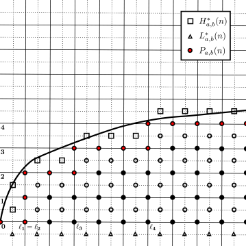
Figure 1: Illustration of $\mathbb{G}_{a,b}(n)$ for $n=10$. The curve is the graph of $f(u)=a\log(1+u)+b\log(1+\log(1+u))$ and vertices of $\mathbb{G}_{a,b}(n)$ are the solid dots (black and red). The vertices of the dual graph are the non-filled circles, squares, and triangles. Those of the “highest path” $P_{a,b}(n)$ are displayed in red, the “top side” of $\mathbb{G}_{a,b}^{\ast}(n)$ is $H_{a,b}^{\ast}(n)$, whose vertices are displayed as squares, and the “bottom side” is $L_{a,b}^{\ast}(n)$, whose vertices are displayed as triangles. The values listed on the $x$-axis are $\ell_{j}$, the smallest value of $u$ for which $f(u)\geq j$. Because $f$ increases sharply near 0 in the figure, we have $f(0)=0$ but $f(1)\geq 2$, so $\ell_{1}=\ell_{2}=1$.

I. Dual representation. In the first part of the proof, we describe a standard representation of $T_{a,b}^{B}(0,P(n))$ in terms of separating sets. We will call an edge $e$ closed if $t_{e}=1$; otherwise, we call it open. A set $U\subset\mathbb{E}_{a,b}(n)$ is said to be closed if all its edges are closed. We say that $U\subset\mathbb{E}_{a,b}(n)$ is a separating set if each path in $\mathbb{G}_{a,b}(n)$ from $0$ to any vertex in $P(n)$ contains an edge in $U$. Define $Y_{n}$ as

$$Y_{n}=\text{maximal number of disjoint closed separating sets}.$$ (3.2)

We claim that

$$T_{a,b}^{B}(0,P(n))=Y_{n}.$$ (3.3)

(This claim also holds for Bernoulli FPP on general graphs, with “separating set” defined suitably.)

To prove (3.3), we start with the inequality $\geq$. If $Y_{n}=0$ then the inequality is trivial; otherwise, let $E_{1},\dots,E_{Y_{n}}$ be a maximal collection of disjoint closed separating sets. If $\gamma$ is a path from $0$ to a vertex in $P(n)$, we can find distinct edges $e_{1}\in E_{1},\dots,e_{Y_{n}}\in E_{Y_{n}}$ that are in $\gamma$ and are closed. Then $T(\gamma)\geq t_{e_{1}}+\dots+t_{e_{Y_{n}}}\geq Y_{n}$. To prove the inequality $\leq$, we must produce $T_{a,b}^{B}(0,P(n))$ many disjoint closed separating sets. Again if $T_{a,b}^{B}(0,P(n))=0$ then the inequality is trivial. Otherwise, for $j=0,\dots,T_{a,b}^{B}(0,P(n))-1$, define $B(j)=\{v\in\mathbb{V}_{a,b}(n):T_{a,b}^{B}(0,v)\leq j\}$ and $E_{j}=\{\{v,w\}\in\mathbb{E}_{a,b}(n):v\in B(j),w\notin B(j)\}$. The $E_{j}$ are disjoint because if $\{v,w\}$ is an edge in $E_{j}$ with $v\in B(j)$ and $w\notin B(j)$, then we have $j<T_{a,b}^{B}(0,w)\leq T_{a,b}^{B}(0,v)+t_{\{v,w\}}\leq j+1$, implying that $w\in B(j+1)\setminus B(j)$. This means that for each $j_{1}<j_{2}$, every edge in $E_{j_{2}}$ has an endpoint in $B(j_{2}+1)\setminus B(j_{2})$, and this therefore cannot be an endpoint of any edge in $E_{j_{1}}$. To show they are separating, fix $j=0,\dots,T_{a,b}^{B}(0,P(n))-1$ and let $\gamma$ be a path from $0$ to a vertex $x\in P(n)$ in $\mathbb{G}_{a,b}(n)$. We have $0\in B(j)$ and because $x\in P(n)$, we have $T_{a,b}^{B}(0,x)\geq T_{a,b}^{B}(0,P(n))>j$, so $x\notin B(j)$. Therefore there is an edge $\{v,w\}$ in $\gamma$ such that $v\in B(j)$ and $w\notin B(j)$, and hence $E_{j}$ is separating. Last, if $\{v,w\}\in E_{j}$ then we must have $t_{\{v,w\}}=1$ because if $t_{\{v,w\}}=0$ we would have $T_{a,b}^{B}(0,v)=T_{a,b}^{B}(0,w)$, which is false. Therefore $\{E_{j}\}$ forms a collection of disjoint closed separating sets, and so $T_{a,b}^{B}(0,P(n))\leq Y_{n}$. This proves (3.3).

Next, we represent $Y_{n}$ using the dual lattice. Let $(\mathbb{Z}^{2})^{\ast}=\mathbb{Z}^{2}+(1/2,1/2)$ be the set of dual vertices and let $(\mathbb{E}^{2})^{\ast}$ be its set of nearest neighbor edges. Each edge $e\in\mathbb{E}^{2}$ is bisected by a unique edge $e^{\ast}\in(\mathbb{E}^{2})^{\ast}$ and we assign this dual edge the same weight as its primal edge by defining $t_{e^{\ast}}=t_{e}$. We say that the dual edge $e^{\ast}$ is open if $t_{e}=0$ and is closed otherwise. The dual graph for $\mathbb{G}_{a,b}(n)$ is $\mathbb{G}_{a,b}^{\ast}(n)$, which has edge set

$$\mathbb{E}_{a,b}^{\ast}(n)=\{e^{\ast}:e\in\mathbb{E}_{a,b}(n)\}$$

and vertex set

$$\mathbb{V}_{a,b}^{\ast}(n)=\{v:v\text{ is an endpoint of an edge of }\mathbb{E}_{a,b}^{\ast}(n)\}.$$

The “top side” of $\mathbb{G}^{\ast}_{a,b}(n)$ is the set of dual vertices that are above the highest path $P_{a,b}(n)$:

$$H_{a,b}^{\ast}(n)=\left\{v\in\mathbb{V}_{a,b}^{\ast}(n):\begin{array}[]{c}v\text{ is an endpoint of }e^{\ast}\text{ for some edge }e\text{ in }P_{a,b}(n)\text{ and }v\text{ lies }\\ \text{above }P_{a,b}(n)\text{ in the strip }\{(x_{1},x_{2})\in\mathbb{R}^{2}:0\leq x_{1}\leq n\}\end{array}\right\}$$

(these vertices are either the top or left endpoints of edges dual to those in $P_{a,b}(n)$), and the “bottom side” is the set $L_{a,b}^{\ast}(n)=\{(1/2,-1/2),\dots,(n-1/2,-1/2)\}$. See Fig. 1 for an illustration of these definitions.

We claim that

$$Y_{n}=\begin{array}[]{c}\text{maximal number of edge-disjoint closed dual }\\ \text{paths in }\mathbb{G}_{a,b}^{\ast}(n)\text{ from }H_{a,b}^{\ast}(n)\text{ to }L_{a,b}^{\ast}(n).\end{array}$$ (3.4)

To prove this, denote the right side by $Y_{n}^{\prime}$. We first show that $Y_{n}\leq Y_{n}^{\prime}$ and observe that it is trivially true if $Y_{n}=0$. Otherwise, let $E_{1},\dots,E_{Y_{n}}$ be a maximal collection of disjoint closed separating sets. Fix $j=1,\dots,Y_{n}$, call each edge in $E_{j}$ “vacant” and each edge in $\mathbb{E}_{a,b}(n)\setminus E_{j}$ “occupied.” A dual edge is called occupied if its corresponding primal edge is occupied; otherwise it is vacant. By planar duality (see [3, p. 55]), either there is a path of occupied edges from $0$ to $P(n)$ in $\mathbb{G}_{a,b}(n)$ or there is a dual path of vacant edges from $H_{a,b}^{\ast}(n)$ to $L_{a,b}^{\ast}(n)$ in $\mathbb{G}_{a,b}^{\ast}(n)$. Because $E_{j}$ is separating, any path of the first type would have to contain a vacant edge, which is impossible. So a dual path of the second type must exist and this shows that $Y_{n}\leq Y_{n}^{\prime}$. The other inequality $Y_{n}\geq Y_{n}^{\prime}$ also follows similarly. Indeed, it is trivial if $Y_{n}^{\prime}=0$; otherwise, if $P_{1},\dots,P_{Y_{n}^{\prime}}$ is a maximal collection of edge-disjoint paths in $\mathbb{G}_{a,b}^{\ast}(n)$ from $H^{\ast}_{a,b}(n)$ to $L_{a,b}^{\ast}(n)$, we may fix $j$ and call all edges of $P_{j}$ “vacant” with all other edges “occupied.” A primal edge is called occupied if its corresponding dual edge is occupied; otherwise it is vacant. Planar duality then implies that there is no occupied path in $\mathbb{G}_{a,b}(n)$ from $0$ to $P(n)$, so any path from $0$ to $P(n)$ must contain a vacant edge. Therefore the edges of $P_{j}$ form a closed separating set, and $Y_{n}\geq Y_{n}^{\prime}$.

II. Upper bounds. Now that we have given our representation for $T_{a,b}^{B}(0,P(n))$ in (3.3) and (3.4), we move to proving the upper bounds. For each $j=0,\dots,\lfloor f(n)\rfloor$, write

$$H_{a,b}^{\ast}(n;j)=\left\{(x_{1},y_{1})\in H_{a,b}^{\ast}(n):y_{1}=j+\frac{1}{2}\right\}.$$

If we define

$$Y_{n,j}=\begin{array}[]{c}\text{maximal number of edge-disjoint closed dual}\\ \text{paths in }\mathbb{G}_{a,b}^{\ast}(n)\text{ from }H_{a,b}^{\ast}(n;j)\text{ to }L_{a,b}^{\ast}(n),\end{array}$$

then from (3.3) and (3.4), we obtain

$$\mathbb{E}T_{a,b}^{B}(0,P(n))\leq\sum_{j=0}^{\lfloor f(n)\rfloor}\mathbb{E}Y_{n,j}.$$ (3.5)

To bound $\mathbb{E}Y_{n,j}$, we need a good estimate on $\#H_{a,b}^{\ast}(n,j)$. For this, we introduce the numbers

$$\ell_{j}=\min\{d\in\mathbb{Z}:d\geq 0\text{ and }f(d)\geq j\}=\lceil f^{-1}(j)\rceil,$$ (3.6)

for $j\geq 0$. This $\ell_{j}$ is the $\mathbf{e}_{1}$-coordinate of the first vertex of the highest path $P_{a,b}(n)$ with $\mathbf{e}_{2}$-coordinate at least equal to $j$. We claim that

$$\#H_{a,b}^{\ast}(n;j)=\begin{cases}\max\{\ell_{j+1}-\ell_{j},1\}&\quad\text{if }j=0,\dots,\lfloor f(n)\rfloor-1\\ n-\ell_{\lfloor f(n)\rfloor}&\quad\text{if }j=\lfloor f(n)\rfloor\\ 0&\quad\text{if }j>\lfloor f(n)\rfloor.\end{cases}$$ (3.7)

To show this, we can describe the motion of $P_{a,b}(n)$ in terms of the $\ell_{j}$’s. Specifically, as we follow the path, we start at $0=(\ell_{0},0)$, move right until $(\ell_{1},0)$ and then up to $(\ell_{1},1)$. Generally, if we are at $(\ell_{j},j)$, we move right (if necessary) to $(\ell_{j+1},j)$, and then up to $(\ell_{j+1},j+1)$. We do this until we reach the point $(\ell_{\lfloor f(n)\rfloor},\lfloor f(n)\rfloor)$, and then move right to $(n,\lfloor f(n)\rfloor)$. The vertices of $H_{a,b}^{\ast}(n;j)$ are either (a) upper endpoints of vertical (dual) edges which are dual to horizontal edges with both endpoints in $\{(x_{1},j):x_{1}\in\mathbb{R}\}$ or (b) left endpoints of horizontal (dual) edges which are dual to vertical edges connecting $\{(x_{1},j):x_{1}\in\mathbb{R}\}$ to $\{(x_{1},j+1):x_{1}\in\mathbb{R}\}$. If $j=0,\dots,\lfloor f(n)\rfloor-1$, the $\ell_{j+1}-\ell_{j}$ many endpoints of type (a) are

$$\left(\ell_{j}+\frac{1}{2},j+\frac{1}{2}\right),\dots,\left(\ell_{j+1}-\frac{1}{2},j+\frac{1}{2}\right)$$

and if $j=\lfloor f(n)\rfloor$, the $n-\ell_{\lfloor f(n)\rfloor}$ many endpoints are

$$\left(\ell_{\lfloor f(n)\rfloor}+\frac{1}{2},\lfloor f(n)\rfloor+\frac{1}{2}\right),\dots,\left(n-\frac{1}{2},\lfloor f(n)\rfloor+\frac{1}{2}\right).$$

The endpoint of type (b) is $(\ell_{j+1}-1/2,j+1/2)$ if $j=0,\dots,\lfloor f(n)\rfloor-1$ (observe that this point has already been counted in the list of type (a) points when $\ell_{j+1}-\ell_{j}>0$) and there are no such endpoints when $j=\lfloor f(n)\rfloor$. If $j>\lfloor f(n)\rfloor$, then there are no endpoints of types (a) or (b). Putting these cases together proves (3.7).

To estimate $\ell_{j}$, we note that for all large $j$, we have

$$\frac{e^{\frac{j}{a}}}{\left(1+\frac{j}{a}\right)^{\frac{b}{a}}}-1\leq f^{-1}(j)\leq\frac{e^{\frac{j}{a}}}{\left(1+\frac{j}{a}\right)^{\frac{b}{a}}}\cdot\left(\frac{1}{1-\frac{b}{a+j}\log\left(1+\frac{j}{a}\right)}\right)^{\frac{b}{a}}-1.$$

This can be verified by applying $f$ to all three terms. Therefore we have

$$\ell_{j}\sim\frac{e^{\frac{j}{a}}}{\left(\frac{j}{a}\right)^{\frac{b}{a}}}\text{ and }(\ell_{j+1}-\ell_{j})\sim(e^{\frac{1}{a}}-1)\frac{e^{\frac{j}{a}}}{\left(\frac{j}{a}\right)^{\frac{b}{a}}},$$ (3.8)

where we use the notation $f_{1}(j)\sim f_{2}(j)$ to mean that $f_{1}(j)\lesssim f_{2}(j)\lesssim f_{1}(j)$.

II(a). Case $p>1/2$. First we suppose that $p>1/2$. Observe that a vertex in the set $H_{a,b}^{\ast}(n;j)$ can be in at most two edge-disjoint dual closed paths in $\mathbb{G}_{a,b}^{\ast}(n)$ and so we have

$$Y_{n,j}\leq 2\#\{v\in H_{a,b}^{\ast}(n;j):v\text{ is connected to }L_{a,b}^{\ast}(n)\text{ in }\mathbb{G}_{a,b}^{\ast}(n)\text{ by a closed dual path}\}.$$

Using this in (3.5) with a union bound, we obtain

$$\mathbb{E}T_{a,b}^{B}(0,P(n)) \leq 2\sum_{j=0}^{\lfloor f(n)\rfloor}\sum_{v\in H_{a,b}^{\ast}(n;j)}\mathbb{P}\left(\begin{array}[]{c}v\text{ is connected to }L_{a,b}^{\ast}(n)\text{ in }\\ \mathbb{G}_{a,b}^{\ast}(n)\text{ by a closed dual path}\end{array}\right)$$

$$\leq 2\sum_{j=0}^{\lfloor f(n)\rfloor}\#H_{a,b}^{\ast}(n;j)\mathbb{P}_{1-p}(0\leftrightarrow P(j+1)).$$

Equation (3.7) and Prop. 2.3 then imply

$$\mathbb{E}T_{a,b}^{B}(0,P(n)) \leq 2\Cr{c:point_{t}o_{p}lane_{u}pper}\sum_{j=0}^{\lfloor f(n)\rfloor-1}\max\{\ell_{j+1}-\ell_{j},1\}\exp\left(-\frac{j+1}{\xi(1-p)}\right)$$

$$+2\Cr{c:point_{t}o_{p}lane_{u}pper}(n-\ell_{\lfloor f(n)\rfloor})\exp\left(-\frac{\lfloor f(n)\rfloor+1}{\xi(1-p)}\right).$$

Due to (3.8), there exists $J_{a,b}$ such that if $j\geq J_{a,b}$ then $\ell_{j+1}-\ell_{j}\geq 1$. This implies that

$$\mathbb{E}T_{a,b}^{B}(0,P(n)) \leq 2\Cr{c:point_{t}o_{p}lane_{u}pper}J_{a,b}$$

$$+2\Cr{c:point_{t}o_{p}lane_{u}pper}\sum_{j=0}^{\lfloor f(n)\rfloor-1}(\ell_{j+1}-\ell_{j})\exp\left(-\frac{j+1}{\xi(1-p)}\right)$$ (3.9)

$$+2\Cr{c:point_{t}o_{p}lane_{u}pper}(n-\ell_{\lfloor f(n)\rfloor})\exp\left(-\frac{\lfloor f(n)\rfloor+1}{\xi(1-p)}\right).$$ (3.10)

For the first term, we use (3.8) to say that

$$\text{if }\sum_{j}\frac{\exp\left(j\left(\frac{1}{a}-\frac{1}{\xi(1-p)}\right)\right)}{j^{\frac{b}{a}}}\text{ diverges,}$$ (3.11)

then

$$\eqref{eq: split_1a}\sim 2\Cr{c:point_{t}o_{p}lane_{u}pper}\left(e^{\frac{1}{a}}-1\right)a^{\frac{b}{a}}e^{-\frac{1}{\xi(1-p)}}\sum_{j=1}^{\lfloor f(n)\rfloor-1}\frac{\exp\left(j\left(\frac{1}{a}-\frac{1}{\xi(1-p)}\right)\right)}{j^{\frac{b}{a}}}.$$ (3.12)

For the second term, if we write

$$\Delta_{a,b}^{(2)}(n)=\frac{n-\ell_{\lfloor f(n)\rfloor}}{n}\exp\left(\frac{f(n)-\lfloor f(n)\rfloor-1}{\xi(1-p)}\right),$$

we have

$$\eqref{eq: split_2a} =2\Cr{c:point_{t}o_{p}lane_{u}pper}\Delta_{a,b}^{(2)}(n)\cdot n\exp\left(-\frac{f(n)}{\xi(1-p)}\right)$$

$$=2\Cr{c:point_{t}o_{p}lane_{u}pper}\Delta_{a,b}^{(2)}(n)\cdot n(1+n)^{-\frac{a}{\xi(1-p)}}(1+\log(1+n))^{-\frac{b}{\xi(1-p)}}$$

$$\sim 2\Cr{c:point_{t}o_{p}lane_{u}pper}\Delta_{a,b}^{(2)}(n)\frac{n^{1-\frac{a}{\xi(1-p)}}}{(\log n)^{\frac{b}{\xi(1-p)}}}.$$ (3.13)

If $a<\xi(1-p)$, then (3.11) holds and we use that for any $\alpha>0$ and $\beta\geq 0$, one has

$$\sum_{\ell=1}^{j}\frac{e^{\alpha\ell}}{\ell^{\beta}}\sim\frac{1}{e^{\alpha}-1}\cdot\frac{e^{\alpha(j+1)}}{j^{\beta}}.$$ (3.14)

This implies from (3.12) that if we write

$$\Delta_{a,b}^{(1)}(n)=\exp\left(-(f(n)-\lfloor f(n)\rfloor)\left(\frac{1}{a}-\frac{1}{\xi(1-p)}\right)\right),$$

then we have

$$\eqref{eq: split_1a} \sim 2\Cr{c:point_{t}o_{p}lane_{u}pper}a^{\frac{b}{a}}\cdot\frac{e^{\frac{1}{a}}-1}{e^{\frac{1}{a}}-e^{\frac{1}{\xi(1-p)}}}\cdot\frac{\exp\left(\lfloor f(n)\rfloor\left(\frac{1}{a}-\frac{1}{\xi(1-p)}\right)\right)}{\left(\lfloor f(n)\rfloor-1\right)^{\frac{b}{a}}}$$

$$\sim 2\Cr{c:point_{t}o_{p}lane_{u}pper}\Delta_{a,b}^{(1)}(n)\cdot\frac{e^{\frac{1}{a}}-1}{e^{\frac{1}{a}}-e^{\frac{1}{\xi(1-p)}}}\cdot\frac{\exp\left(f(n)\left(\frac{1}{a}-\frac{1}{\xi(1-p)}\right)\right)}{(\log n)^{\frac{b}{a}}}$$

$$=2\Cr{c:point_{t}o_{p}lane_{u}pper}\Delta_{a,b}^{(1)}(n)\cdot\frac{e^{\frac{1}{a}}-1}{e^{\frac{1}{a}}-e^{\frac{1}{\xi(1-p)}}}\cdot\frac{(1+n)^{1-\frac{a}{\xi(1-p)}}(1+\log(1+n))^{b\left(\frac{1}{a}-\frac{1}{\xi(1-p)}\right)}}{(\log n)^{\frac{b}{a}}}$$

$$\sim 2\Cr{c:point_{t}o_{p}lane_{u}pper}\Delta_{a,b}^{(1)}(n)\left(1+\frac{e^{\frac{1}{\xi(1-p)}}-1}{e^{\frac{1}{a}}-e^{\frac{1}{\xi(1-p)}}}\right)\frac{n^{1-\frac{a}{\xi(1-p)}}}{(\log n)^{\frac{b}{\xi(1-p)}}}.$$ (3.15)

In summary, when $p>1/2$ and $a<\xi(1-p)$, we have from (3.13) and (3.15) that

$$\eqref{eq: split_1a}+\eqref{eq: split_2a}\sim 2\Cr{c:point_{t}o_{p}lane_{u}pper}\left(\Delta_{a,b}^{(1)}(n)\left(1+\frac{e^{\frac{1}{\xi(1-p)}}-1}{e^{\frac{1}{a}}-e^{\frac{1}{\xi(1-p)}}}\right)+\Delta_{a,b}^{(2)}(n)\right)\frac{n^{1-\frac{a}{\xi(1-p)}}}{(\log n)^{\frac{b}{\xi(1-p)}}}.$$ (3.16)

Using $|\Delta_{a,b}^{(1)}(n)|\leq 1$, $|\Delta_{a,b}^{(2)}(n)|\leq 1$, and

$$\frac{e^{\frac{1}{\xi(1-p)}}-1}{e^{\frac{1}{a}}-e^{\frac{1}{\xi(1-p)}}}=\frac{1-e^{-\frac{1}{\xi(1-p)}}}{e^{\frac{1}{a}-\frac{1}{\xi(1-p)}}-1}\leq\frac{1}{e^{\frac{1}{a}-\frac{1}{\xi(1-p)}}-1}\leq\frac{1}{\frac{1}{a}-\frac{1}{\xi(1-p)}}\leq\frac{\xi(1-p)^{2}}{\xi(1-p)-a},$$

we find

$$\mathbb{E}T_{a,b}^{B}(0,P(n))\lesssim 2\Cr{c:point_{t}o_{p}lane_{u}pper}\left(2+\frac{\xi(1-p)^{2}}{\xi(1-p)-a}\right)\frac{n^{1-\frac{a}{\xi(1-p)}}}{(\log n)^{\frac{b}{\xi(1-p)}}}.$$

The prefactor is bounded above by $C_{p}/(\xi(1-p)-a)$ for a $p$-dependent constant $C_{p}$, so this implies the upper bound in the theorem in this case.

If, instead, we have $b<a=\xi(1-p)$, then (3.11) still holds and we can use $\sum_{\ell=1}^{j}\ell^{-\alpha}\sim j^{1-\alpha}/(1-\alpha)$ for $\alpha<1$ in (3.12) to produce

$$\eqref{eq: split_1a}\sim 2\Cr{c:point_{t}o_{p}lane_{u}pper}\left(e^{\frac{1}{a}}-1\right)a^{\frac{b}{a}}e^{-\frac{1}{\xi(1-p)}}\sum_{j=1}^{\lfloor f(n)\rfloor-1}\frac{1}{j^{\frac{b}{a}}} \sim 2\Cr{c:point_{t}o_{p}lane_{u}pper}\frac{1-e^{-\frac{1}{\xi(1-p)}}}{1-\frac{b}{\xi(1-p)}}a^{\frac{b}{a}}\cdot\left(\lfloor f(n)\rfloor-1\right)^{1-\frac{b}{a}}$$

$$\sim 2\Cr{c:point_{t}o_{p}lane_{u}pper}\xi(1-p)\frac{1-e^{-\frac{1}{\xi(1-p)}}}{1-\frac{b}{\xi(1-p)}}\left(\log n\right)^{1-\frac{b}{\xi(1-p)}}.$$

Also, from (3.13), we have $\eqref{eq: split_2a}\to 0$ as $n\to\infty$. Therefore if $p>1/2$ and $b<a=\xi(1-p)$, then

$$\eqref{eq: split_1a}+\eqref{eq: split_2a}\sim 2\Cr{c:point_{t}o_{p}lane_{u}pper}\xi(1-p)\frac{1-e^{-\frac{1}{\xi(1-p)}}}{1-\frac{b}{\xi(1-p)}}\left(\log n\right)^{1-\frac{b}{\xi(1-p)}}.$$ (3.17)

This implies the upper bound in the theorem in this case.

Next, if $a=b=\xi(1-p)$, then (3.11) holds and (3.12) implies that

$$\eqref{eq: split_1a}\sim 2\Cr{c:point_{t}o_{p}lane_{u}pper}a\left(1-e^{-\frac{1}{\xi(1-p)}}\right)\sum_{j=1}^{\lfloor f(n)\rfloor-1}\frac{1}{j}\sim 2\Cr{c:point_{t}o_{p}lane_{u}pper}a\left(1-e^{-\frac{1}{\xi(1-p)}}\right)\log\log n.$$

From (3.13), we have $\eqref{eq: split_2a}\to 0$ as $n\to\infty$. Therefore if $p>1/2$ and $a=b=\xi(1-p)$, then we have

$$\eqref{eq: split_1a}+\eqref{eq: split_2a}\sim 2\Cr{c:point_{t}o_{p}lane_{u}pper}a\left(1-e^{-\frac{1}{\xi(1-p)}}\right)\log\log n$$ (3.18)

and this is the upper bound in the theorem in this case.

Last, if $a>\xi(1-p)$, or if $a=\xi(1-p)$ but $b>\xi(1-p)$, then (3.11) fails. Because $\ell_{j+1}-\ell_{j}\sim(e^{1/a}-1)e^{j/a}/(j/a)^{b/a}$, this immediately implies that (3.9) converges. Also $\eqref{eq: split_2a}\to 0$ as $n\to\infty$, so $\sup_{n}\mathbb{E}T_{a,b}^{B}(0,P(n))<\infty$, as claimed.

II(b). Case $p=1/2$. Next we suppose that $p=1/2$ and return to the estimate (3.5) for $\mathbb{E}T_{a,b}^{B}(0,P(n))$ in terms of the variables $Y_{n,j}$. Unlike in the case $p>1/2$, we cannot just bound $Y_{n,j}$ by the number of vertices in $H^{\ast}_{a,b}(n;j)$ that are connected to $L_{a,b}^{\ast}(n)$. When $p=1/2$, many such vertices will correspond to the same closed dual path because large critical clusters touch $H^{\ast}_{a,b}(n;j)$ many times, but also have cut-edges. To deal with this, we use some standard critical percolation constructions.

To stay close to the results in Sec. 2, we will temporarily switch to open paths rather than closed dual ones (this does not matter because $p=1/2$). For integers $n$ and $h(n)$, let

$$U(h(n),n)=\begin{array}[]{c}\text{maximal number of edge-disjoint open paths }\\ \text{from }\left(\{0\}\times[0,h(n)]\right)\cap\mathbb{Z}^{2}\text{ to }P(n).\end{array}$$ (3.19)

These open paths are allowed to use any edges in $\mathbb{E}^{2}$. We will show that there exists $\Cl[lgc]{c:critical_{u}pper}>0$ such that for all $n$ and all choices of $h(n)\geq n$, we have

$$\mathbb{E}U(h(n),n)\leq\Cr{c:critical_{u}pper}\frac{h(n)}{n}.$$ (3.20)

To prove this, we first consider the case $h(n)=n$. Any open path from $(\{0\}\times[0,n])\cap\mathbb{Z}^{2}$ to $P(n)$ must contain a left-right crossing of $B_{1}$ or $B_{2}$, or contain a top-down crossing of $B_{3}$ or $B_{4}$, where the $B_{i}$ are defined as follows:

$$B_{1}=\left([0,n]\times[-n,2n]\right)\cap\mathbb{Z}^{2},~B_{2}=B_{1}-n\mathbf{e}_{1},$$

and

$$B_{3}=\left([-2n,n]\times[n,2n]\right)\cap\mathbb{Z}^{2},~B_{4}=B_{3}-2n\mathbf{e}_{2}.$$

By symmetry, we obtain

$$\mathbb{E}U(n,n)\leq 4\mathbb{E}\left(\text{maximal number of edge-disjoint left-right open crossings of }B_{1}\right).$$

By the RSW theorem (see [14, Eq. (11.74),(11.76)]), there exists $\Cl[smc]{c:RSW1}>0$ such that for all $n$, we have

$$\mathbb{P}(B_{1}\text{ has a left-right open crossing})\leq 1-\Cr{c:RSW1}.$$

As in (2.8), we apply to BK inequality to obtain

$$\mathbb{E}\left(\text{maximal number of edge-disjoint left-right open crossings of }B_{1}\right)\leq\frac{1-\Cr{c:RSW1}}{\Cr{c:RSW1}},$$

and so $\mathbb{E}U(n,n)\leq 4(1-\Cr{c:RSW1})/\Cr{c:RSW1}$. This shows (3.20) in the case $h(n)=n$. If $h(n)>n$, we simply write $U_{n}(j)$ for the maximal number of edge-disjoint open paths from $(\{0\}\times[(j-1)n,jn])\cap\mathbb{Z}^{2}$ to $P(n)$ and observe that by symmetry, we have

$$\mathbb{E}U(h(n),n)\leq\sum_{j=1}^{\left\lfloor\frac{h(n)}{n}\right\rfloor+1}\mathbb{E}U_{n}(j)\leq\left(\frac{h(n)}{n}+1\right)\mathbb{E}U(n,n)\leq\frac{8(1-\Cr{c:RSW1})}{\Cr{c:RSW1}}\cdot\frac{h(n)}{n},$$

proving (3.20).

We now return to (3.5) and to using closed dual paths. Because $p=1/2$, we have

$$\mathbb{E}Y_{n,j}\leq\mathbb{E}U(\#H_{a,b}^{\ast}(n;j),j+1),$$

and so using (3.7), we find

$$\mathbb{E}T_{a,b}^{B}(0,P(n))\leq\sum_{j=0}^{\lfloor f(n)\rfloor-1}\mathbb{E}U(\max\{\ell_{j+1}-\ell_{j},1\},j+1)+\mathbb{E}U(n-\ell_{\lfloor f(n)\rfloor},\lfloor f(n)\rfloor+1).$$

The second summand is bounded by $\mathbb{E}U(n,\lfloor f(n)\rfloor+1)$. Because $\ell_{j+1}-\ell_{j}\geq j+1$ for $j$ sufficiently large (depending on $a$ and $b$) and $n\geq\lfloor f(n)\rfloor+1$ for $n$ sufficiently large, (3.20) implies that for some $K_{a,b}>0$, we have

$$\mathbb{E}T_{a,b}^{B}(0,P(n))\leq K_{a,b}+\sum_{j=0}^{\lfloor f(n)\rfloor-1}\Cr{c:critical_{u}pper}\frac{\ell_{j+1}-\ell_{j}}{j+1}+\Cr{c:critical_{u}pper}\frac{n}{\lfloor f(n)\rfloor+1},$$

if $n$ is large enough. Using (3.8) and the fact that $\sum_{j}e^{j/a}/(j/a)^{b/a+1}$ diverges for all $a>0$ and $b\geq 0$, we get

$$\mathbb{E}T_{a,b}^{B}(0,P(n)) \lesssim\Cr{c:critical_{u}pper}\left(e^{\frac{1}{a}}-1\right)\sum_{j=1}^{\lfloor f(n)\rfloor-1}\frac{e^{\frac{j}{a}}}{\left(\frac{j}{a}\right)^{\frac{b}{a}}(j+1)}+\Cr{c:critical_{u}pper}\frac{n}{a\log n}$$

$$\lesssim\Cr{c:critical_{u}pper}\left(e^{\frac{1}{a}}-1\right)a^{\frac{b}{a}}\sum_{j=1}^{\lfloor f(n)\rfloor-1}\frac{e^{\frac{j}{a}}}{j^{\frac{b}{a}+1}}+\Cr{c:critical_{u}pper}\frac{n}{a\log n}$$

Again (3.14) implies

$$\mathbb{E}T_{a,b}^{B}(0,P(n)) \lesssim\Cr{c:critical_{u}pper}a^{\frac{b}{a}}\cdot\frac{e^{\frac{\lfloor f(n)\rfloor}{a}}}{\left(\lfloor f(n)\rfloor-1\right)^{\frac{b}{a}+1}}+\Cr{c:critical_{u}pper}\frac{n}{a\log n}$$

$$\lesssim\Cr{c:critical_{u}pper}\frac{(1+n)(1+\log(1+n))^{\frac{b}{a}}}{a\left(\log n\right)^{\frac{b}{a}+1}}+\Cr{c:critical_{u}pper}\frac{n}{a\log n}$$

$$\lesssim 2\Cr{c:critical_{u}pper}\frac{n}{a\log n}.$$

This completes the proof of the upper bound in the case $p=1/2$.

III. Lower bounds. For lower bounds, we look at top-down dual closed crossings of rectangles.

III(a). Case $p>1/2$. In this case, we use rectangles that are contained in $\mathbb{G}_{a,b}^{\ast}(n)$, defining $R_{a,b}^{\ast}(n;j)$ to have top side equal to $H_{a,b}^{\ast}(n;j)$: for any $j$ such that $\ell_{j+1}>\ell_{j}$, we set

$$R_{a,b}^{\ast}(n;j)=\left(\left[\ell_{j}+\frac{1}{2},\ell_{j+1}-\frac{1}{2}\right]\times\left[-\frac{1}{2},j+\frac{1}{2}\right]\right)\cap(\mathbb{Z}^{2})^{\ast}.$$

There exists $J_{a,b}$ such that

$$\text{for }j\geq J_{a,b}\text{ we have }\ell_{j+1}-\ell_{j}-1\geq 6(j+1),$$ (3.21)

and so, in particular, for $j=J_{a,b},\dots,\lfloor f(n)\rfloor-1$, the set $R_{a,b}^{\ast}(n;j)$ is defined. The final rectangle is

$$R_{a,b}^{\ast}(n;\lfloor f(n)\rfloor)=\left(\left[\ell_{\lfloor f(n)\rfloor}+\frac{1}{2},n-\frac{1}{2}\right]\times\left[-\frac{1}{2},\lfloor f(n)\rfloor+\frac{1}{2}\right]\right)\cap(\mathbb{Z}^{2})^{\ast}.$$

For $j=J_{a,b},\dots,\lfloor f(n)\rfloor$, let

$$X_{n,j}=\text{maximal number of edge-disjoint closed dual top-down crossings of }R_{a,b}^{\ast}(n;j).$$

Because any top-down crossing of $R_{a,b}^{\ast}(n;j)$ starts in $H_{a,b}^{\ast}(n)$ and ends in $L_{a,b}^{\ast}(n)$, and the $R_{a,b}^{\ast}(n;j)$ are disjoint, we have from (3.3) and (3.4) that

$$\mathbb{E}T_{a,b}^{B}(0,P(n))\geq\sum_{j=J_{a,b}}^{\lfloor f(n)\rfloor}\mathbb{E}X_{n,j}.$$

Because of (3.21), we may apply Cor. 2.6 to the rectangle $R_{a,b}^{\ast}(n;j)$ to get

$$\mathbb{E}X_{n,j}\geq\Cr{c:crossing_{n}umber_{l}ower_{n}ew}(\ell_{j+1}-\ell_{j}-1)\exp\left(-\frac{j+1}{\xi(1-p)}\right)\text{ for }j=J_{a,b},\dots,\lfloor f(n)\rfloor-1,$$

and for $j=\lfloor f(n)\rfloor$, if $n-\ell_{\lfloor f(n)\rfloor}-1\geq 6(\lfloor f(n)\rfloor+1)$, we have

$$\mathbb{E}X_{n,\lfloor f(n)\rfloor}\geq\Cr{c:crossing_{n}umber_{l}ower_{n}ew}(n-\ell_{\lfloor f(n)\rfloor})\exp\left(-\frac{\lfloor f(n)\rfloor+1}{\xi(1-p)}\right).$$

On the other hand, if $n-\ell_{\lfloor f(n)\rfloor}\leq 6(\lfloor f(n)\rfloor+1)$, the right side of the above display is bounded above by $6\Cr{c:crossing_{n}umber_{l}ower_{n}ew}(\lfloor f(n)\rfloor+1)e^{-(\lfloor f(n)\rfloor+1)/\xi(1-p)}$, which tends to zero as $n\to\infty$. Putting these together, we obtain a constant $K_{a,b,p}$ depending on $a,b$, and $p$ such that

$$\mathbb{E}T_{a,b}^{B}(0,P(n)) \geq\sum_{j=J_{a,b}}^{\lfloor f(n)\rfloor-1}\Cr{c:crossing_{n}umber_{l}ower_{n}ew}(\ell_{j+1}-\ell_{j}-1)\exp\left(-\frac{j+1}{\xi(1-p)}\right)$$

$$+\Cr{c:crossing_{n}umber_{l}ower_{n}ew}(n-\ell_{\lfloor f(n)\rfloor})\exp\left(-\frac{\lfloor f(n)\rfloor+1}{\xi(1-p)}\right)$$

$$-6\Cr{c:crossing_{n}umber_{l}ower_{n}ew}(\lfloor f(n)\rfloor+1)e^{-(\lfloor f(n)\rfloor+1)/\xi(1-p)}$$

$$\geq-K_{a,b,p}$$

$$+\Cr{c:crossing_{n}umber_{l}ower_{n}ew}\sum_{j=0}^{\lfloor f(n)\rfloor-1}(\ell_{j+1}-\ell_{j})\exp\left(-\frac{j+1}{\xi(1-p)}\right)$$

$$+\Cr{c:crossing_{n}umber_{l}ower_{n}ew}(n-\ell_{\lfloor f(n)\rfloor})\exp\left(-\frac{\lfloor f(n)\rfloor+1}{\xi(1-p)}\right)$$

$$=-K_{a,b,p}+\frac{\Cr{c:crossing_{n}umber_{l}ower_{n}ew}}{2\Cr{c:point_{t}o_{p}lane_{u}pper}}\cdot\left(\eqref{eq: split_1a}+\eqref{eq: split_2a}\right).$$ (3.22)

If $p>1/2$ and $b<a=\xi(1-p)$, then the lower bound in the theorem follows directly from (3.17) and (3.22). Similarly, if $p>1/2$ and $a=b=\xi(1-p)$, then the lower bound in the theorem follows directly from (3.18) and (3.22). We may therefore suppose that $a<\xi(1-p)$ and may use (3.16) in (3.22) to find

$$\mathbb{E}T_{a,b}^{B}(0,P(n))\gtrsim\Cr{c:crossing_{n}umber_{l}ower_{n}ew}\left(\Delta_{a,b}^{(1)}(n)\left(1+\frac{e^{\frac{1}{\xi(1-p)}}-1}{e^{\frac{1}{a}}-e^{\frac{1}{\xi(1-p)}}}\right)+\Delta_{a,b}^{(2)}(n)\right)\frac{n^{1-\frac{a}{\xi(1-p)}}}{(\log n)^{\frac{b}{\xi(1-p)}}}.$$

To finish the lower bound in the case $p>1/2$ and $a<\xi(1-p)$, we may show that for some constant $\Cl[smc]{c:my_{f}avorite_{c}onstant}=\Cr{c:my_{f}avorite_{c}onstant}(p)>0$, we have

$$\Delta_{a,b}^{(1)}(n)\left(1+\frac{e^{\frac{1}{\xi(1-p)}}-1}{e^{\frac{1}{a}}-e^{\frac{1}{\xi(1-p)}}}\right)+\Delta_{a,b}^{(2)}(n)\gtrsim\frac{\Cr{c:my_{f}avorite_{c}onstant}}{\xi(1-p)-a}.$$ (3.23)

If $n\geq 2\ell_{\lfloor f(n)\rfloor}$, then

$$\Delta_{a,b}^{(2)}(n)\geq\frac{1}{2}\exp\left(\frac{f(n)-\lfloor f(n)\rfloor-1}{\xi(1-p)}\right)\geq\frac{1}{2}\exp\left(-\frac{1}{\xi(1-p)}\right).$$

On the other hand, if $n\leq 2\ell_{\lfloor f(n)\rfloor}$, then we can show that $\Delta_{a,b}^{(1)}(n)\gtrsim 1/2$ by using the following facts. First, we have

$$\lfloor f(n)\rfloor-f(\ell_{\lfloor f(n)\rfloor})\to 0\text{ as }n\to\infty.$$ (3.24)

This follows because $f(\ell_{j})\geq j$ for $j\geq 0$ and $f(\ell_{j}-1)<j$ when $\ell_{j}\geq 1$, and so for large $n$, we have

$$\lfloor f(n)\rfloor\leq f(\ell_{\lfloor f(n)\rfloor})<f(\ell_{\lfloor f(n)\rfloor})-f(\ell_{\lfloor f(n)\rfloor}-1)+\lfloor f(n)\rfloor.$$

Because of our choice of $f$, we have $f(\ell_{\lfloor f(n)\rfloor})-f(\ell_{\lfloor f(n)\rfloor}-1)\to 0$ as $n\to\infty$, and so this gives (3.24).

Next, because $n\lesssim e^{\frac{1}{a}}\ell_{\lfloor f(n)\rfloor}$, we have $\ell_{\lfloor f(n)\rfloor}\leq n\leq C_{a,b}\ell_{\lfloor f(n)\rfloor}$ for some constant $C_{a,b}$ depending on $a$ and $b$, and so

$$|f(n)-f(\ell_{\lfloor f(n)\rfloor})-\left(a\log n-a\log\ell_{\lfloor f(n)\rfloor}\right)|$$

$$\leq~ a\bigg{|}\log\left(\frac{1+n}{n}\right)-\log\left(\frac{1+\ell_{\lfloor f(n)\rfloor}}{\ell_{\lfloor f(n)\rfloor}}\right)\bigg{|}+b\bigg{|}\log\left(\frac{1+\log(1+n)}{1+\log(1+\ell_{\lfloor f(n)\rfloor})}\right)\bigg{|}$$

$$\leq~ a\bigg{|}\log\left(\frac{1+n}{n}\right)-\log\left(\frac{1+\ell_{\lfloor f(n)\rfloor}}{\ell_{\lfloor f(n)\rfloor}}\right)\bigg{|}+b\bigg{|}\log\left(\frac{1+\log(1+C_{a,b}\ell_{\lfloor f(n)\rfloor})}{1+\log(1+\ell_{\lfloor f(n)\rfloor})}\right)\bigg{|}$$

$$\to~ 0\text{ as }n\to\infty.$$

This, along with (3.24), implies that

$$\Delta_{a,b}^{(1)}(n) \sim\exp\left(-(f(n)-f(\ell_{\lfloor f(n)\rfloor}))\left(\frac{1}{a}-\frac{1}{\xi(1-p)}\right)\right)$$

$$\sim\exp\left(-(a\log n-a\log\ell_{\lfloor f(n)\rfloor})\left(\frac{1}{a}-\frac{1}{\xi(1-p)}\right)\right)$$

$$=\exp\left(-\left(\log\frac{n}{\ell_{\lfloor f(n)\rfloor}}\right)\left(1-\frac{a}{\xi(1-p)}\right)\right)$$

$$\geq\frac{1}{2}.$$

Therefore $\Delta_{a,b}^{(1)}(n)+\Delta_{a,b}^{(2)}(n)\gtrsim e^{-1/\xi(1-p)}/2$ and so

$$\Delta_{a,b}^{(1)}(n)\left(1+\frac{e^{\frac{1}{\xi(1-p)}}-1}{e^{\frac{1}{a}}-e^{\frac{1}{\xi(1-p)}}}\right)+\Delta_{a,b}^{(2)}(n)$$

$$\gtrsim~ \Delta_{a,b}^{(1)}(n)\left(\frac{e^{\frac{1}{\xi(1-p)}}-1}{e^{\frac{1}{a}}-e^{\frac{1}{\xi(1-p)}}}\right)+\frac{1}{2}\exp\left(-\frac{1}{\xi(1-p)}\right)$$

$$\geq~ \exp\left(-\left(\frac{1}{a}-\frac{1}{\xi(1-p)}\right)\right)\left(\frac{e^{\frac{1}{\xi(1-p)}}-1}{e^{\frac{1}{a}}-e^{\frac{1}{\xi(1-p)}}}\right)+\frac{1}{2}\exp\left(-\frac{1}{\xi(1-p)}\right).$$

If $a<\xi(1-p)/2$, then we drop the first term to see that this expression is $\geq e^{-1/\xi(1-p)}/2\geq c_{p}/(\xi(1-p)-a)$, with $c_{p}=e^{-1/\xi(1-p)}\xi(1-p)/4$. On the other hand, if $a\geq\xi(1-p)/2$, then we drop the second term, giving a lower bound for the expression of

$$\exp\left(-\frac{2}{\xi(1-p)}\right)\left(\exp\left(\frac{1}{\xi(1-p)}\right)-1\right)\cdot\frac{1}{e^{\frac{1}{a}-\frac{1}{\xi(1-p)}}-1}$$

which is bounded below by $c_{p}/(\xi(1-p)-a)$ for a (more complicated) constant $c_{p}$ depending only on $p$, assuming that $a$ remains bigger than $\xi(1-p)/2$. These two cases imply (3.23) and complete the proof of the lower bound when $p>1/2$.

III(b). Case $p=1/2$. Last, we prove the lower bound in the case $p=1/2$ and show, like in (3.20), that if

$$V(h(n),n)=\begin{array}[]{c}\text{maximal number of edge-disjoint left-right open}\\ \text{crossings of }([0,n]\times[0,h(n)])\cap\mathbb{Z}^{2},\end{array}$$

then for some constant $\Cl[smc]{c:critical_{l}ower_{c}onstant}>0$, we have

$$\mathbb{E}V(h(n),n)\geq\Cr{c:critical_{l}ower_{c}onstant}\frac{h(n)}{n}$$ (3.25)

for all choices of $n$ and $h(n)\geq n$. To do this, we make a packing by squares. Set $B_{1}=([0,n]\times[0,n])\cap\mathbb{Z}^{2}$, $B_{2}=([0,n]\times[n+1,2n+1])\cap\mathbb{Z}^{2}$, and in general, for $j\geq 1$, set

$$B_{j}=([0,n]\times[(j-1)(n+1),j(n+1)-1])\cap\mathbb{Z}^{2}.$$

The final square $B_{j}$ which fits inside of our rectangle has index $j_{0}=\lfloor(h(n)+1)/(n+1)\rfloor$. Using [14, p. 316], we have $\mathbb{P}(B_{1}\text{ has a left-right open crossing})\geq 1/2$, and so (3.25) follows:

$$\mathbb{E}V(h(n),n)\geq\sum_{j=1}^{j_{0}}\mathbb{P}(B_{j}\text{ has a left-right open crossing})\geq\frac{j_{0}}{2}\geq\frac{1}{8}\cdot\frac{h(n)}{n}.$$

To use (3.25), we observe that if we define the dual rectangle

$$R_{a,b}^{\ast}(n)=\left(\left[\frac{1}{2},n-\frac{1}{2}\right]\times\left[-\frac{1}{2},\lfloor f(n)\rfloor+\frac{1}{2}\right]\right)\cap(\mathbb{Z}^{2})^{\ast},$$

then every top-down dual crossing of $R_{a,b}^{\ast}(n)$ contains a dual path from $H_{a,b}^{\ast}(n)$ to $L_{a,b}^{\ast}(n)$. Therefore $Y_{n}$, defined back in (3.4), satisfies

$$Y_{n}\geq\text{maximal number of edge-disjoint top-down closed dual crossings of }R_{a,b}^{\ast}(n).$$

Because $n-1\geq\lfloor f(n)\rfloor+1$ for all large $n$, we can use (3.25) to conclude that

$$\mathbb{E}T_{a,b}^{B}(0,P(n))\geq\mathbb{E}V(n-1,\lfloor f(n)\rfloor+1)\gtrsim\Cr{c:critical_{l}ower_{c}onstant}\frac{n-1}{\lfloor f(n)\rfloor+1}\gtrsim\Cr{c:critical_{l}ower_{c}onstant}\frac{n}{a\log n},$$

completing the proof.

4 Martingale construction for general wedges

The proofs of both Thm. 1.5 and Thm. 1.6 use the martingale construction of Kesten-Zhang [18], replacing their open circuits in annuli with open top-down crossings of the sets $R_{i}$. It will be more convenient for us to have the $R_{i}$ separated by blank space, so we will work only with the even indices, which correspond to the sets $R_{2i}$ for $i\geq 0$. To avoid endless confusion, we set $r_{i}^{\prime}=r_{2i}$ and $R_{i}^{\prime}=R_{2i}$ for $i\geq 0$. From here on, we use the coupling of $(\tau_{e})$ and $(t_{e})$ defined at the beginning of Sec. 3, and we assume A1-A3 for some $\Cr{c:r_{i}{}_{a}ssumption_{1}}>0$, $\Cr{c:r_{i}{}_{a}ssumption_{2}}\in[1,\infty)$, and $\Cr{c:r_{i}{}_{a}ssumption_{3}}:[0,\infty)\to(0,\infty)$. Therefore we may choose an integer $i^{\ast}\geq 1$ such that

$$\mathbb{P}(\exists~\text{top-down open crossing of }R_{i})\geq\frac{\Cr{c:r_{i}{}_{a}ssumption_{1}}}{2}\text{ for }i\geq 2i^{\ast},$$ (4.1)

and

$$\mathbb{E}T_{f}^{B}(0,P(r_{i+1})-\mathbb{E}T_{f}^{B}(0,P(r_{i}))\leq 2\Cr{c:r_{i}{}_{a}ssumption_{2}}\text{ for }i\geq i^{\ast}.$$ (4.2)

The next few sections develop the martingale construction, and the proofs of Thm. 1.5 and Thm. 1.6 will be given in Sec. 4.6.

4.1 Line-to-line bound

Before we give the main definitions, we prove a tail bound on the passage time between lines $P(r_{i}^{\prime})$ and $P(r_{j}^{\prime})$ for $i<j$ that will be applied throughout. We first observe that (4.2) implies that for integers $i,j$ with $i^{\ast}\leq i<j$, we have

$$\mathbb{E}T_{f}^{B}(P(r_{i}^{\prime}),P(r_{j}^{\prime})) \leq\mathbb{E}\left[T_{f}^{B}(0,P(r_{j}^{\prime}))-T_{f}^{B}(0,P(r_{i}^{\prime}))\right]$$

$$=\sum_{\ell=2i}^{2j-1}\left[\mathbb{E}T_{f}^{B}(0,P(r_{\ell+1}))-\mathbb{E}T_{f}^{B}(0,P(r_{\ell}))\right]$$

$$\leq 4\Cr{c:r_{i}{}_{a}ssumption_{2}}(j-i).$$ (4.3)

(In fact, (4.3) is a weaker version of A2 that suffices for our purposes.) The following corresponds to [18, Eq. (2.50)].

Lemma 4.1.

There exist $\Cl[lgc]{c:haydns_{c}onstant_{1}}\geq 1$ and $\Cl[smc]{c:haydns_{c}onstant_{2}}>0$ depending only on $\Cr{c:r_{i}{}_{a}ssumption_{2}}$ such that for all integers $i,j$ with $i^{\ast}\leq i<j$ and $y\geq 0$, we have

$$\mathbb{P}(T_{f}(P(r_{i}^{\prime}),P(r_{j}^{\prime}))\geq y)\leq\Cr{c:haydns_{c}onstant_{1}}\exp\left(-\Cr{c:haydns_{c}onstant_{2}}\frac{y}{j-i}\right)+\frac{\Cr{c:haydns_{c}onstant_{1}}}{y^{\frac{\eta}{2}}}.$$

Proof.

Let $z\geq 0$ be an integer and write

$$\mathbb{P}(T_{f}(P(r_{i}^{\prime}),P(r_{j}^{\prime}))\geq y) \leq\mathbb{P}(T_{f}^{B}(P(r_{i}^{\prime}),P(r_{j}^{\prime}))\geq z)$$ (4.4)

$$+\mathbb{P}(T_{f}^{B}(P(r_{i}^{\prime}),P(r_{j}^{\prime}))<z,T_{f}(P(r_{i}^{\prime}),P(r_{j}^{\prime}))\geq y).$$ (4.5)

For (4.4), we first use (4.3) and Markov’s inequality to obtain

$$\mathbb{P}(T_{f}^{B}(P(r_{i}^{\prime}),P(r_{j}^{\prime}))\geq 8\Cr{c:r_{i}{}_{a}ssumption_{2}}(j-i))\leq\frac{1}{2}.$$ (4.6)

Next observe that, similarly to (3.2), we have

$$T_{f}^{B}(P(r_{i}^{\prime}),P(r_{j}^{\prime}))=\begin{array}[]{c}\text{maximal number of disjoint closed sets in }\mathbb{E}_{f}\text{ separating }\\ \{r_{i}^{\prime}\}\times\{0,\dots,\lfloor f(r_{i}^{\prime})\rfloor\}\text{ from }\{r_{j}^{\prime}\}\times\{0,\dots,\lfloor f(r_{j}^{\prime})\rfloor\}.\end{array}$$ (4.7)

As in (3.3), these separating sets are defined as edge sets in $\mathbb{E}_{f}$ such that each path in $\mathbb{G}_{f}$ starting in $\{r_{i}^{\prime}\}\times\{0,\dots,\lfloor f(r_{i}^{\prime})\rfloor\}$ and ending in $\{r_{j}^{\prime}\}\times\{0,\dots,\lfloor f(r_{j}^{\prime})\rfloor\}$ must contain an edge in the separating set. If $m\geq 0$ is an integer and $T_{f}^{B}(P(r_{i}^{\prime}),P(r_{j}^{\prime}))\geq m\lceil 8\Cr{c:r_{i}{}_{a}ssumption_{2}}(j-i)\rceil$, then we can find $m$ disjoint edge sets, each of which contains at least $\lceil 8\Cr{c:r_{i}{}_{a}ssumption_{2}}(j-i)\rceil$ many disjoint separating sets. By the BK inequality and (4.6),

$$\mathbb{P}(T_{f}^{B}(P(r_{i}^{\prime}),P(r_{j}^{\prime}))\geq m\lceil 8\Cr{c:r_{i}{}_{a}ssumption_{2}}(j-i)\rceil) \leq\mathbb{P}(\exists~\lceil 8\Cr{c:r_{i}{}_{a}ssumption_{2}}(j-i)\rceil\text{ many disjoint separating sets})^{m}$$

$$\leq 2^{-m},$$

and so

$$\text{RHS of }\eqref{eq: plane_to_plane_term_1} =\mathbb{P}\left(T_{f}^{B}(P(r_{i}^{\prime}),P(r_{j}^{\prime}))\geq\frac{z}{\lceil 8\Cr{c:r_{i}{}_{a}ssumption_{2}}(j-i)\rceil}\lceil 8\Cr{c:r_{i}{}_{a}ssumption_{2}}(j-i)\rceil\right)$$

$$\leq 2^{-\lfloor\frac{z}{\lceil 8\Cr{c:r_{i}{}_{a}ssumption_{2}}(j-i)\rceil}\rfloor}$$

$$\leq\Cl[lgc]{c:trainor_{c}onstant_{1}}\exp\left(-\Cl[smc]{c:trainor_{c}onstant_{2}}\frac{z}{j-i}\right),$$ (4.8)

for some $\Cr{c:trainor_{c}onstant_{1}},\Cr{c:trainor_{c}onstant_{2}}>0$ depending only on $\Cr{c:r_{i}{}_{a}ssumption_{2}}$.

As for (4.5), we write

$$\eqref{eq: plane_to_plane_term_2}=\sum_{k=0}^{z-1}\mathbb{E}\left[\mathbb{P}\left(T_{f}(P(r_{i}^{\prime}),P(r_{j}^{\prime}))\geq y\mid(t_{e})\right)\mathbf{1}_{\{T_{f}^{B}(P(r_{i}^{\prime}),P(r_{j}^{\prime}))=k\}}\right],$$ (4.9)

where $\mathbb{P}(\cdot\mid(t_{e}))$ represents the conditional probability given the Bernoulli weights $(t_{e})$. On the event $\{T_{f}^{B}(P(r_{i}^{\prime}),P(r_{j}^{\prime}))=k\}$, we can choose an optimal path for $T_{f}^{B}(P(r_{i}^{\prime}),P(r_{j}^{\prime}))$ (in some $(t_{e})$-measurable way, for example by picking the first such optimal path in a deterministic ordering of all finite paths in $\mathbb{Z}^{2}$) and write $e_{1},\dots,e_{k}$ for the $k$ many edges listed in order along the path that satisfy $t_{e_{i}}=1$ for all $i$. If $T_{f}(P(r_{i}^{\prime}),P(r_{j}^{\prime}))\geq y$, then it must be that $\tau_{e_{1}}^{\prime}+\dots+\tau_{e_{k}}^{\prime}=\tau_{e_{1}}+\dots+\tau_{e_{k}}\geq y$ (recall the coupling $\tau_{e}=t_{e}\tau_{e}^{\prime}$ from below (1.6)), so

$$\eqref{eq: plane_to_plane_term_2} \leq\sum_{k=0}^{z-1}\sum_{f_{1},\dots,f_{k}}\mathbb{E}\left[\mathbb{P}\left(\tau_{f_{1}}^{\prime}+\dots+\tau_{f_{k}}^{\prime}\geq y\mid(t_{e})\right)\mathbf{1}_{\{T_{f}^{B}(P(r_{i}^{\prime}),P(r_{j}^{\prime}))=k\}}\mathbf{1}_{\{e_{i}=f_{i}~\forall i\}}\right]$$

$$\leq\sum_{k=0}^{z-1}\sum_{f_{1},\dots,f_{k}}\mathbb{P}(\tau_{1}^{\prime}+\dots+\tau_{k}^{\prime}\geq y)\mathbb{P}(T_{f}^{B}(P(r_{i}^{\prime}),P(r_{j}^{\prime}))=k,e_{i}=f_{i}~\forall i)$$

$$\leq\mathbb{P}(\tau_{1}^{\prime}+\dots+\tau_{z}^{\prime}\geq y),$$

where the second inequality uses independence of $(\tau_{e}^{\prime})$ from $(t_{e})$, and the variables $\tau_{1}^{\prime},\dots,\tau_{z}^{\prime}$ are i.i.d., with the same common distribution as $(\tau_{e}^{\prime})$. So long as

$$y\geq 2z\mathbb{E}\tau_{1}^{\prime},$$ (4.10)

we have

$$\mathbb{P}(\tau_{1}^{\prime}+\dots+\tau_{z}^{\prime}\geq y) \leq\mathbb{P}\left(|\tau_{1}^{\prime}-\mathbb{E}\tau_{1}^{\prime}+\dots+\tau_{z}^{\prime}-\mathbb{E}\tau_{z}^{\prime}|\geq\frac{y}{2}\right)$$

$$\leq 2^{\eta}y^{-\eta}\mathbb{E}|\tau_{1}^{\prime}+\dots+\tau_{z}^{\prime}-\mathbb{E}[\tau_{1}^{\prime}+\dots+\tau_{z}^{\prime}]|^{\eta}.$$

By applying [15, Thm. I.5.1(iii)] and noting that $\mathbb{E}(\tau_{k}^{\prime})^{\eta}<\infty$ by (1.6) (and that $\eta>4\geq 2$), we obtain an upper bound of

$$\eqref{eq: plane_to_plane_term_2}\leq 2^{\eta}y^{-\eta}\Cl[lgc]{c:guts_{c}onstant}z^{\frac{\eta}{2}}\mathbb{E}|\tau_{1}^{\prime}|^{\eta}\leq 2^{\eta}y^{-\eta}\Cr{c:guts_{c}onstant}\left(\frac{y}{2\mathbb{E}\tau_{1}^{\prime}}\right)^{\frac{\eta}{2}}\mathbb{E}|\tau_{1}^{\prime}|^{\eta},$$

for some universal $\Cr{c:guts_{c}onstant}$ depending only on $\eta$. In the second inequality, we used (4.10). In total, this gives $\Cl[lgc]{c:guts_{c}onstant_{2}}$ depending only on $\eta$ and the distribution of $\tau_{e}$ such that for all $i,j$ with $0\leq i<j$ and all $y$ satisfying (4.10), we have

$$\eqref{eq: plane_to_plane_term_2}\leq\frac{\Cr{c:guts_{c}onstant_{2}}}{y^{\frac{\eta}{2}}}.$$

If we then set $z=\lfloor y/(2\mathbb{E}\tau_{1}^{\prime})\rfloor$, then the previous display holds, and we can combine it with (4.8) to deduce that

$$\mathbb{P}(T_{f}(P(r_{i}^{\prime}),P(r_{j}^{\prime}))(\omega)\geq y)\leq\Cr{c:trainor_{c}onstant_{1}}\exp\left(-\Cr{c:trainor_{c}onstant_{2}}\frac{\lfloor\frac{y}{2\mathbb{E}\tau_{1}^{\prime}}\rfloor}{j-i}\right)+\frac{\Cr{c:guts_{c}onstant_{2}}}{y^{\frac{\eta}{2}}},$$

which implies the statement of the lemma. ∎

The proof of Lem. 4.1 requires $\int x^{2}~\text{d}F(x)<\infty$ to apply [15, Thm. I.5.1(iii)], and this holds because of (1.6). We remark that the bound in the lemma can be improved under the assumption that

$$f(m)\geq 3\text{ for }m=r_{i}^{\prime},\dots,r_{j}^{\prime}\text{ and }\int x^{\eta}~\text{d}F(x)<\infty\text{ for some }\eta>2/3.$$

In this case, one can show that given $s\in[2,3\eta)$, there exist $\Cr{c:haydns_{c}onstant_{1}}\geq 1$ and $\Cr{c:haydns_{c}onstant_{2}}>0$ depending only on $\Cr{c:r_{i}{}_{a}ssumption_{2}}$ such that for all integers $i,j$ with $i^{\ast}\leq i<j$ and $y\geq 0$, we have

$$\mathbb{P}(T_{f}(P(r_{i}^{\prime}),P(r_{j}^{\prime}))\geq y)\leq\Cr{c:haydns_{c}onstant_{1}}\exp\left(-\Cr{c:haydns_{c}onstant_{2}}\frac{y}{j-i}\right)+\frac{\Cr{c:haydns_{c}onstant_{1}}}{y^{\frac{s}{2}}}.$$ (4.11)

In the rest of this subsection, we outline the modifications needed to obtain this stronger inequality. This result is not used in the paper except to justify Rem. 5 about the optimal moment condition for Thm. 1.3. The proof is the same as that of Lem. 4.1 until we reach (4.9), and then differs by providing a better upper bound for the conditional probability appearing in the sum of that equation.

To do this, for any edge $e\in\mathbb{E}_{f}$, we define two edge sets $S_{k}(e)$ for $k=1,2$ that surround $e$ as follows. First taking $e=\{(0,0),(1,0)\}$, we define $S_{1}(e)$ as the set of edges with both endpoints in the (topological) boundary of $[0,1]\times[-1,1]$, and $S_{2}(e)$ as the set of edges with both endpoints in the (topological) boundary of the rectangle $[-1,2]\times[-2,2]$. If $e\in\mathbb{E}_{f}$ is another horizontal edge, we define $S_{k}(e)$ by translating the definition of $S_{k}(\{(0,0),(1,0)\})$ in such a way that $(0,0)$ is mapped to the left endpoint of $e$. In case $e$ is a vertical edge, we rotate these definitions by $\pi/2$.

For $e\in\mathbb{E}_{f}$, let $m_{e}^{(0)}=\tau_{e}^{\prime},m_{e}^{(k)}=\sum_{f\in S_{k}(e)}\tau_{f}^{\prime}$, for $k=1,2$, and $m_{e}=\min_{k=0,1,2}m_{e}^{(k)}$. We claim that

$$T_{f}(P(r_{i}^{\prime}),P(r_{j}^{\prime}))\leq\left(\sum_{\ell=1}^{k}m_{e_{\ell}}\right)\text{ on the event }\{T_{f}^{B}(P(r_{i}^{\prime}),P(r_{j}^{\prime}))=k\},$$ (4.12)

where, like after (4.9), we have chosen an optimal path for $T_{f}^{B}(P(r_{i}^{\prime}),P(r_{j}^{\prime}))$ in some $(t_{e})$-measurable way and listed $e_{1},\dots,e_{k}$ as the $k$ many edges in order along along the path that satisfy $t_{e_{i}}=1$ for all $i$. The strategy to show (4.12) is to choose $i_{1},\dots,i_{k}\in\{0,1,2\}$ and construct a path $\Gamma_{0}$ in $\mathbb{G}_{f}$ that connects $P(r_{i}^{\prime})$ to $P(r_{j}^{\prime})$ but satisfies

$$T_{f}(\Gamma_{0})\leq\sum_{\ell=1}^{k}m_{e_{\ell}}^{(i_{\ell})}.$$ (4.13)

The path $\Gamma_{0}$ is constructed by following $\Gamma$ but, because the sets $S_{k}(e)$ surround $e$ for $k=1,2$, taking a detour through $S_{i_{\ell}}(e_{\ell})$ for $\ell=1,\dots,k$ instead of taking the edge $e_{\ell}$ whenever $i_{\ell}\neq 0$. This construction appears to require several cases because $f$ is general, but it is always possible assuming that $f(m)\geq 3$ for all $m=r_{i}^{\prime},\dots,r_{j}^{\prime}$. (If $f(m)\leq 2$ then the set $S_{e}(k)$ may separate $P(r_{i}^{\prime})$ from $P(r_{j}^{\prime})$ and intersections of $\Gamma$ with the set of endpoints of edges in $S_{e}(k)$ may not be connectable through $S_{e}(k)$ using only edges of $\mathbb{G}_{f}$.) Because (4.13) holds for all choices of $i_{1},\dots,i_{k}\in\{0,1,2\}$, this implies (4.12).

Given (4.12), we can continue from (4.9) by writing

$$\eqref{eq: plane_to_plane_term_2} \leq\sum_{k=0}^{z-1}\sum_{f_{1},\dots,f_{k}}\mathbb{E}\left[\mathbb{P}\left(m_{f_{1}}+\dots+m_{f_{k}}\geq y\mid(t_{e})\right)\mathbf{1}_{\{T_{f}^{B}(P(r_{i}^{\prime}),P(r_{j}^{\prime}))=k\}}\mathbf{1}_{\{e_{i}=f_{i}~\forall i\}}\right].$$

We observe that $\mathbb{E}\left(m_{e}^{(k)}\right)^{\eta}<\infty$ for $k=0,1,2$ and furthermore that the $m_{e}^{(k)}$ are independent as $k$ varies and $e$ is fixed. Therefore for $s<3\eta$, we can apply Markov’s inequality and independence to obtain for some $\mathsf{C}>0$

$$\mathbb{E}m_{e}^{s}=\int_{0}^{\infty}sy^{s-1}\mathbb{P}(m_{e}\geq y)~\text{d}y =\int_{0}^{\infty}sy^{s-1}\prod_{k=0}^{3}\mathbb{P}\left(m_{e}^{(k)}\geq y\right)~\text{d}y$$

$$\leq\mathsf{C}\int_{0}^{\infty}sy^{s-1}\cdot\frac{\text{d}y}{y^{3\eta}}<\infty.$$

The $m_{e}$ are not independent, but they are only finitely dependent, so if $s\in[2,3\eta)$, we can still apply a version of [15, Thm. I.5.1(iii)] to obtain for $k\leq z$ and some constants $\mathsf{C}$

$$\mathbb{P}(m_{f_{1}}+\dots+m_{f_{k}}\geq y\mid(t_{e})) =\mathbb{P}(m_{f_{1}}+\dots+m_{f_{k}}\geq y)$$

$$\leq 2^{s}y^{-s}\mathbb{E}|m_{f_{1}}+\dots+m_{f_{k}}-\mathbb{E}[m_{f_{1}}+\dots+m_{f_{k}}]|^{s}$$

$$\leq 2^{s}y^{-s}\mathsf{C}z^{\frac{s}{2}}\mathbb{E}m_{e}^{s}$$

$$\leq\frac{\mathsf{C}}{y^{\frac{s}{2}}},$$

assuming that $y\geq 2z\mathbb{E}m_{e}$ (compare to (4.10)). We can then follow to the end of the proof of Lem. 4.1 to obtain (4.11).

4.2 Martingale definitions

For $i\geq 0$, define

$$m(i)=\min\{j\geq i:R_{j}^{\prime}\text{ has a top-down open crossing}\}.$$

We observe that if $R_{i}^{\prime}$ has a top-down open crossing, it also has a top-down open crossing that is vertex self-avoiding, and when viewed as a plane curve, any such crossing is simple. To every simple curve $\Gamma$ connecting $\{(x_{1},x_{2})\in\mathbb{R}^{2}:x_{2}=f(x_{1})\}$ to $\{(x_{1},x_{2})\in\mathbb{R}^{2}:x_{1}\geq 0,x_{2}=0\}$ within the region $\{(x_{1},x_{2})\in\mathbb{R}^{2}:0\leq x_{2}\leq f(x_{1})\}$ we can associate an interior

$$\text{int }\Gamma=\text{ bounded component of }\{(x_{1},x_{2})\in\mathbb{R}^{2}:0\leq x_{2}\leq f(x_{1})\}\setminus\Gamma$$

and an exterior

$$\text{ext }\Gamma=\text{ unbounded component of }\{(x_{1},x_{2})\in\mathbb{R}^{2}:0\leq x_{2}\leq f(x_{1})\}\setminus\Gamma.$$

We say that a path $\Gamma$ is the leftmost top-down open crossing of $R_{i}^{\prime}$ if it is a vertex self-avoiding top-down open crossing of $R_{i}^{\prime}$ and, when viewed as a plane curve, $\text{int }\Gamma$ is minimal among all vertex self-avoiding top-down open crossings of $R_{i}^{\prime}$.

Figure 2: Illustration of the definitions involved in the martingale construction. In the figure, the top solid curve is the graph of $f$ and the region below the curve and between $r_{i-1}^{\prime}=r_{2i-2}$ and $r_{2i-1}$ is $R_{i-1}^{\prime}$. The dotted curves connecting the top solid curve to the bottom are open paths. There is no top-down open crossing of $R_{i-1}^{\prime}$, so $m(i-1)>i-1$. The region to the right of $r_{i}^{\prime}$ below the graph of $f$ is $R_{i}^{\prime}$, and it has a top-down open crossing, so $m(i-1)=m(i)=i$ and the leftmost such crossing is labeled as $\Gamma_{i-1}$, which is also equal to $\Gamma_{i}$. The middle two open paths connecting the top solid curve to the bottom are not contained in any $R_{j}^{\prime}$, so they do not affect the values of $m(i-1),m(i),\Gamma_{i-1},\Gamma_{i}$.

By assumption A1, we have $i\leq m(i)<\infty$ almost surely for each $i\geq 0$. We can therefore define

$$\Gamma_{i}=\text{ leftmost top-down open crossing of }R_{m(i)}^{\prime}\text{ for }i\geq 0.$$

(See Fig. 2 for an illustration of $\Gamma_{i}$.) Next we define the sigma-algebra $\Sigma_{i}$ that contains the information about (a) what $\Gamma_{i}$ is and (b) what the weights $(\tau_{e})$ are on and to the left of $\Gamma_{i}$. For any vertex self-avoiding top-down crossing $\Gamma$ of $R_{j}^{\prime}$ for some $j\geq i$, any finite subset $E$ of $\mathbb{E}_{f}$ all whose endpoints are in $\Gamma\cup\text{int }\Gamma$, and any Borel set $B\subset\mathbb{R}^{\#E}$, define the event $\Xi_{i}(\Gamma,E,B)$ as

$$\Xi_{i}(\Gamma,E,B)=\{\Gamma_{i}=\Gamma\}\cap\{(t_{e})_{e\in E}\in B\}.$$

Last, we set $\Sigma_{-1}=\{\emptyset,\Omega\}$, and

$$\Sigma_{i}=\sigma\left(\{\Xi_{i}(\Gamma,E,B)\}_{\Gamma,E,B}\right)\text{ for }i\geq 0,$$

as $\Gamma,E,B$ range over the items satisfying the conditions above. Regarding these definitions, one can check that

$$\Sigma_{i}\subset\Sigma_{i+1}\text{ for }i\geq-1$$

and

$$T_{f}(0,\Gamma_{i})\text{ is }\Sigma_{i}\text{-measurable for }i\geq 0,$$

so long as we set $T_{f}(0,\Gamma_{i})=\infty$ on the probability zero set $\{m(i)=\infty\}$ on which $\Gamma_{i}$ is not defined.

Regarding these definitions, we have the following preliminary bounds. First, there exists $\Cl[smc]{c:circuit_{a}ppearance_{c}onstant}>0$ depending only on $\Cr{c:r_{i}{}_{a}ssumption_{1}}$ such that

$$\mathbb{P}(m(i)\geq i+t)\leq e^{-\Cr{c:circuit_{a}ppearance_{c}onstant}t}\text{ for all integers }i\geq i^{\ast}\text{ and }t\geq 0.$$ (4.14)

To show this, we directly use (4.1) and independence. If $m(i)\geq i+t$, then there can be no top-down open crossing of any of the regions $R_{i}^{\prime},R_{i+1}^{\prime},\dots,R_{i+t-1}^{\prime}$, so by independence, we have

$$\mathbb{P}(m(i)\geq i+t)=\mathbb{P}\left(\bigcap_{t^{\prime}=0}^{t-1}\{\exists\text{ top-down open crossing of }R_{i+t^{\prime}}^{\prime}\}^{c}\right)\leq\left(1-\frac{\Cr{c:r_{i}{}_{a}ssumption_{1}}}{2}\right)^{t},$$

and this implies (4.14).

Second, Lem. 4.1 and (4.14) imply that

$$\mathbb{E}T_{f}(0,\Gamma_{i})^{2}<\infty\text{ for all }i\geq 0.$$ (4.15)

Indeed, for $x\geq 0$, we have

$$\mathbb{P}(T_{f}(0,\Gamma_{i})\geq x)\leq\mathbb{P}(m(i)\geq i+\lfloor\sqrt{x}\rfloor)+\mathbb{P}(T_{f}(P(r_{0}^{\prime}),P(r_{i+\lfloor\sqrt{x}\rfloor}^{\prime}))\geq x).$$

If we write $\Xi$ for the sum of $\tau_{e}$ over all $e\in\mathbb{E}_{f}$ with an endpoint in $S(r_{i^{\ast}}^{\prime})$ (where $S(n)$ was defined in (2.1)), we have

$$T_{f}(P(r_{0}^{\prime}),P(r_{i+\lfloor\sqrt{x}\rfloor}^{\prime}))\leq\Xi+T_{f}(P(r_{i^{\ast}}^{\prime}),P(r_{i+\lfloor\sqrt{x}\rfloor}^{\prime}))\text{ for }i\geq 0\text{ and }x\geq(i^{\ast})^{2}.$$ (4.16)

Therefore for $x\geq(i^{\ast}+1)^{2}$, we can use Lem. 4.1 and (4.14) to obtain

$$\mathbb{P}(T_{f}(0,\Gamma_{i})\geq x) \leq e^{-\Cr{c:circuit_{a}ppearance_{c}onstant}\lfloor\sqrt{x}\rfloor}+\mathbb{P}\left(\Xi\geq\frac{x}{2}\right)+\mathbb{P}\left(T_{f}(P(r_{i^{\ast}}^{\prime}),P(r_{i+\lfloor\sqrt{x}\rfloor}^{\prime}))\geq\frac{x}{2}\right)$$

$$\leq e^{-\Cr{c:circuit_{a}ppearance_{c}onstant}\lfloor\sqrt{x}\rfloor}+\mathbb{P}\left(\Xi\geq\frac{x}{2}\right)+\Cr{c:haydns_{c}onstant_{1}}\exp\left(-\Cr{c:haydns_{c}onstant_{2}}\frac{x}{2(i+\lfloor\sqrt{x}\rfloor-i^{\ast})}\right)+\Cr{c:haydns_{c}onstant_{1}}\left(\frac{2}{x}\right)^{\frac{\eta}{2}}.$$ (4.17)

Multiplying by $x$, integrating over $x$, and noting that (1.6) implies $\mathbb{E}\Xi^{2}<\infty$ gives (4.15).

Most of the proof consists of proving variance bounds and a CLT for $T_{f}(0,\Gamma_{i_{0}})$ as $i_{0}\to\infty$, and then using these results to prove similar ones for $T_{f}(0,P(n))$ with $n\geq 0$. For this purpose, we let $i_{0}\geq 0$ and decompose

$$T_{f}(0,\Gamma_{i_{0}})-\mathbb{E}T_{f}(0,\Gamma_{i_{0}}) =\sum_{i=0}^{i_{0}}\left(\mathbb{E}\left[T_{f}(0,\Gamma_{i_{0}})\mid\Sigma_{i}\right]-\mathbb{E}\left[T_{f}(0,\Gamma_{i_{0}})\mid\Sigma_{i-1}\right]\right)$$

$$:=\sum_{i=0}^{i_{0}}\Delta_{i,i_{0}}.$$

Because of (4.15), we have $\mathrm{Var}~T_{f}(0,\Gamma_{i_{0}})=\sum_{i=0}^{i_{0}}\mathbb{E}\Delta_{i,i_{0}}^{2}$.

4.3 Representations for $\Delta_{i,i_{0}}$

To study the variables $\Delta_{i,i_{0}}$, we give the following representation that is analogous to [18, Lem. 1]. For its statement, we introduce a second copy $(\Omega^{\prime},\Sigma^{\prime},\mathbb{P}^{\prime})$ of the original probability space, writing a typical element of $\Omega$ as $\omega$ and a typical element of $\Omega^{\prime}$ as $\omega^{\prime}$. Until the end of Sec. 4.4, we will include $\omega$ or $\omega^{\prime}$ in the previous notation, so $m(i,\omega)$ or $\Gamma_{i}(\omega)$, for example, means $m(i)$ or $\Gamma_{i}$ evaluated in the outcome $\omega$.

Our formula will differ from that in [18] because of the appearance of events $E_{i,i_{0}}$ and $E_{i-1,i_{0}}$, where

$$E_{i,i_{0}}=\{m(i,\omega)<i_{0}\}$$

It seems that these $E_{i}$ are needed also in the statements of [18, Lem. 1] and [18, Lem. 2], but their absence does not provide a major problem in the later arguments of that reference. As in [18], the formula also involves terms like $\mathbb{E}^{\prime}T_{f}(\Gamma_{i}(\omega),\Gamma_{i_{0}}(\omega^{\prime}))(\omega^{\prime})$ which can be thought of as follows. We first fix the outcome $\omega$, and therefore the path $\Gamma_{i}(\omega)$. Next, we choose $\omega^{\prime}$ and therefore the path $\Gamma_{i_{0}}(\omega^{\prime})$. Last, we evaluate the passage time from the set $\Gamma_{i}(\omega)$ to the set $\Gamma_{i_{0}}(\omega^{\prime})$ in the edge-weights associated to the outcome $\omega^{\prime}$, and integrate over $\omega^{\prime}$. The term is therefore a function only of $\omega$.

Lemma 4.2.

For every $i_{0}\geq 0$, and $i=0,\dots,i_{0}$, we have

$$\Delta_{i,i_{0}}(\omega)=\begin{cases}T_{f}(\Gamma_{i-1}(\omega),\Gamma_{i}(\omega))(\omega)+\mathbf{1}_{E_{i,i_{0}}}\mathbb{E}^{\prime}T_{f}(\Gamma_{i}(\omega),\Gamma_{i_{0}}(\omega^{\prime}))(\omega^{\prime})\\ \hskip 112.0187pt-\mathbf{1}_{E_{i-1,i_{0}}}\mathbb{E}^{\prime}T_{f}(\Gamma_{i-1}(\omega),\Gamma_{i_{0}}(\omega^{\prime}))(\omega^{\prime})&\text{ if }i=1,\dots,i_{0},\\ T_{f}(0,\Gamma_{0}(\omega))(\omega)+\mathbf{1}_{E_{0,i_{0}}}\mathbb{E}^{\prime}T_{f}(\Gamma_{0}(\omega),\Gamma_{i_{0}}(\omega^{\prime}))(\omega^{\prime})\\ \hskip 81.66545pt-\mathbb{E}^{\prime}T_{f}(0,\Gamma_{i_{0}}(\omega^{\prime}))(\omega^{\prime})&\text{ if }i=0.\end{cases}$$

Also if $g$ is a deterministic function such that $g(i)\geq i$ for all $i\geq 0$ and if

$$0\leq i_{1}<\dots<i_{K}\leq i_{0}\text{ and }i_{k+1}\geq g(i_{k})+2\text{ for all }k,$$

then the variables $(\Delta_{i_{k},i_{0}}(\omega)\mathbf{1}_{\{m(i_{k},\omega)\leq g(i_{k})\}})_{1\leq k\leq K}$ are independent.

Proof.

We first prove that for $i_{0}\geq 0$ and $j=0,\dots,i_{0}$, we have

$$\mathbb{E}[T_{f}(\Gamma_{j}(\omega),\Gamma_{i_{0}}(\omega))(\omega)\mid\Sigma_{j}]=\mathbf{1}_{E_{j,i_{0}}}\mathbb{E}^{\prime}T_{f}(\Gamma_{j}(\omega),\Gamma_{i_{0}}(\omega^{\prime}))(\omega^{\prime}).$$ (4.18)

The right side is $\Sigma_{j}$-measurable, since it depends on $\omega$ only through $\Gamma_{j}(\omega)$, so we must show that for any relevant $\Gamma,E,B$, we have

$$\mathbb{E}T_{f}(\Gamma_{j}(\omega),\Gamma_{i_{0}}(\omega))(\omega)\mathbf{1}_{\Xi_{j}(\Gamma,E,B)}=\mathbb{E}\left[\mathbf{1}_{E_{j,i_{0}}}\mathbb{E}^{\prime}T_{f}(\Gamma_{j}(\omega),\Gamma_{i_{0}}(\omega^{\prime}))(\omega^{\prime})\mathbf{1}_{\Xi_{j}(\Gamma,E,B)}\right].$$ (4.19)

If $\Gamma$ has all vertices $u$ with $u\cdot\mathbf{e}_{1}\geq r_{i_{0}}^{\prime}$, then

$$\Xi_{j}(\Gamma,E,B)\subset\{\Gamma_{j}(\omega)=\Gamma\}\subset E_{j,i_{0}}^{c}$$

and $\Xi_{j}(\Gamma,E,B)\subset\{\Gamma_{j}(\omega)=\Gamma_{i_{0}}(\omega)\}$. This implies that both sides of (4.19) are zero and so (4.19) holds. Otherwise, all vertices $u$ of $\Gamma$ have $u\cdot\mathbf{e}_{1}<r_{i_{0}}^{\prime}$ (there is no other possibility since $\Gamma$ is a top-down crossing of some $R_{i}^{\prime}$), and the left side of (4.19) is

$$\mathbb{E}T_{f}(\Gamma,\Gamma_{i_{0}}(\omega))(\omega)\mathbf{1}_{\Xi_{j}(\Gamma,E,B)}=\sum_{\Delta}\mathbb{E}T_{f}(\Gamma,\Delta)(\omega)\mathbf{1}_{\Xi_{j}(\Gamma,E,B)}\mathbf{1}_{\{\Gamma_{i_{0}}(\omega)=\Delta\}},$$

where the sum is over all vertex self-avoiding top-down crossings $\Delta$ of $R_{\ell}^{\prime}$ for some $\ell\geq i_{0}$. The event $\Xi_{j}(\Gamma,E,B)$ depends on values of $\tau_{e}$ for $e$ with both endpoints on $\Gamma$ or in its interior. On the other hand, $T_{f}(\Gamma,\Delta)$ depends on $\tau_{e}$ for $e$ with at least one endpoint in the exterior of $\Gamma$. The event $\{\Gamma_{i_{0}}(\omega)=\Delta\}$ depends on $\tau_{e}$ for $e$ with both endpoints in $\{u:u\cdot\mathbf{e}_{1}\geq r_{i_{0}}^{\prime}\}$, which is a subset of $\text{ext }\Gamma$. By independence, the above equals

$$\sum_{\Delta}\mathbb{E}T_{f}(\Gamma,\Delta)(\omega)\mathbf{1}_{\{\Gamma_{i_{0}}(\omega)=\Delta\}}\mathbb{E}\mathbf{1}_{\Xi_{j}(\Gamma,E,B)} =\mathbb{E}^{\prime}T_{f}(\Gamma,\Gamma_{i_{0}}(\omega^{\prime}))(\omega^{\prime})\mathbb{E}\mathbf{1}_{\Xi_{j}(\Gamma,E,B)}$$

$$=\mathbb{E}\left[\mathbf{1}_{\Xi_{j}(\Gamma,E,B)}\mathbb{E}^{\prime}T_{f}(\Gamma_{j}(\omega),\Gamma_{i_{0}}(\omega^{\prime}))(\omega^{\prime})\right]$$

In this case, $\Xi_{j}(\Gamma,E,B)\subset E_{j,i_{0}}$, so this equals the right side of (4.19). We conclude that (4.18) holds.

To finish the proof of the equation in Lem. 4.2, we use (4.18) to write for $i_{0}\geq 0$ and $i=1,\dots,i_{0}$

$$\mathbb{E}[T_{f}(0,\Gamma_{i_{0}}(\omega))(\omega)\mid\Sigma_{i}] =\mathbb{E}[T_{f}(0,\Gamma_{i-1}(\omega))(\omega)\mid\Sigma_{i}]+\mathbb{E}[T_{f}(\Gamma_{i-1}(\omega),\Gamma_{i}(\omega))(\omega)\mid\Sigma_{i}]$$

$$+\mathbb{E}[T_{f}(\Gamma_{i}(\omega),\Gamma_{i_{0}}(\omega))(\omega)\mid\Sigma_{i}]$$

$$=T_{f}(0,\Gamma_{i-1}(\omega))(\omega)+T_{f}(\Gamma_{i-1}(\omega),\Gamma_{i}(\omega))(\omega)$$

$$+\mathbf{1}_{E_{i,i_{0}}}\mathbb{E}^{\prime}T_{f}(\Gamma_{i}(\omega),\Gamma_{i_{0}}(\omega^{\prime}))(\omega^{\prime}).$$

For $i_{0}\geq 0$ and $i=0$, we similarly write

$$\mathbb{E}[T_{f}(0,\Gamma_{i_{0}}(\omega))(\omega)\mid\Sigma_{0}]=T_{f}(0,\Gamma_{0}(\omega))(\omega)+\mathbf{1}_{E_{0,i_{0}}}\mathbb{E}^{\prime}T_{f}(\Gamma_{0}(\omega),\Gamma_{i_{0}}(\omega^{\prime}))(\omega^{\prime}).$$

In the case $i\geq 1$, we use the previous two displays with $i,i-1$ to prove the formula for Lem. 4.2. In the case $i=0$ we use the second display along with the fact that $\mathbb{E}[T_{f}(0,\Gamma_{i_{0}}(\omega))(\omega)\mid\Sigma_{-1}]=\mathbb{E}^{\prime}T_{f}(0,\Gamma_{i_{0}}(\omega^{\prime}))(\omega^{\prime})$ to complete the proof.

For the independence claim, we observe that for $i_{0}\geq 0$ and $i=1,\dots,i_{0}$,

$$\Delta_{i,i_{0}}(\omega)\mathbf{1}_{\{m(i,\omega)\leq g(i)\}}\text{ depends only on }\tau_{e}\text{ for }e\in\mathcal{E}_{i},$$ (4.20)

where

$$\mathcal{E}_{i}=\{e:e\text{ has both endpoints in }\{u:r_{i-1}^{\prime}\leq u\cdot\mathbf{e}_{1}\leq r_{2g(i)+1}\}\}.$$

To see why, observe that $\{m(i,\omega)\leq g(i)\}$ depends only on $\tau_{e}$ for $e\in\mathcal{E}_{i}$ and if this event occurs, then both paths $\Gamma_{i-1}(\omega)$ and $\Gamma_{i}(\omega)$ have all their edges (and all edges in the region between them) in $\mathcal{E}_{i}$. Therefore $T_{f}(\Gamma_{i-1}(\omega),\Gamma_{i}(\omega))(\omega)\mathbf{1}_{\{m(i,\omega)\leq g(i)\}}$ depends only on $\tau_{e}$ for $e\in\mathcal{E}_{i}$. The same is true for the variables $\mathbf{1}_{\{m(i,\omega)\leq g(i)\}}\mathbb{E}^{\prime}T_{f}(\Gamma_{i-1}(\omega),\Gamma_{i_{0}}(\omega^{\prime}))(\omega^{\prime})$ and $\mathbf{1}_{\{m(i,\omega)\leq g(i)\}}\mathbb{E}^{\prime}T_{f}(\Gamma_{i}(\omega),\Gamma_{i_{0}}(\omega^{\prime}))(\omega^{\prime})$. Last, the events $E_{i,i_{0}}$ and $E_{i-1,i_{0}}$ are determined by the values of $m(i,\omega)$ and $m(i-1,\omega)$, and when $\{m(i,\omega)\leq g(i)\}$ occurs, these are determined by $\tau_{e}$ for $e\in\mathcal{E}_{i}$. We conclude that (4.20) holds. In the case $i_{0}\geq 0$ and $i=0$, (4.20) also holds, by similar reasoning, so long as we set

$$\mathcal{E}_{0}=\{e:e\text{ has both endpoints in }\{u:0\leq u\cdot\mathbf{e}_{1}\leq r_{2g(0)+1}\}\}.$$

The independence claim follows directly from (4.20). Indeed, if $0\leq i_{0}<\dots<i_{K}\leq i_{0}$ and $i_{k+1}\geq g(i_{k})+2$ for all $k$, then the edge sets $\mathcal{E}_{i_{k}}$ for $k=1,\dots,K$ are disjoint. Therefore $(\Delta_{i,i_{0}}(\omega)\mathbf{1}_{\{m(i_{k},\omega)\leq g(i_{k})\}})_{1\leq k\leq K}$ are independent. ∎

Next, following [18, Lem. 2], we give an alternative representation for $\Delta_{i,i_{0}}(\omega)$.

Lemma 4.3.

Define

$$\lambda(i,\omega,\omega^{\prime})=m(m(i,\omega)+1,\omega^{\prime}).$$

Then for every $i_{0}\geq 0$ and $i=1,\dots,i_{0}$, we have

$$\Delta_{i,i_{0}}(\omega) =T_{f}(\Gamma_{i-1}(\omega),\Gamma_{i}(\omega))(\omega)$$

$$+\mathbf{1}_{E_{i-1,i_{0}}\cap E_{i,i_{0}}}\left[\mathbb{E}^{\prime}T_{f}(\Gamma_{i}(\omega),\Gamma_{\lambda(i,\omega,\omega^{\prime})}(\omega^{\prime}))(\omega^{\prime})-\mathbb{E}^{\prime}T_{f}(\Gamma_{i-1}(\omega),\Gamma_{\lambda(i,\omega,\omega^{\prime})}(\omega^{\prime}))(\omega^{\prime})\right]$$

$$-\mathbf{1}_{E_{i-1,i_{0}}\setminus E_{i,i_{0}}}\mathbb{E}^{\prime}T_{f}(\Gamma_{i-1}(\omega),\Gamma_{i_{0}}(\omega^{\prime}))(\omega^{\prime}).$$

In the case $i=0$, for every $i_{0}\geq 0$, we have

$$\Delta_{0,i_{0}}(\omega) =T_{f}(0,\Gamma_{0}(\omega))(\omega)$$

$$+\mathbf{1}_{E_{0,i_{0}}}\left[\mathbb{E}^{\prime}T_{f}(\Gamma_{0}(\omega),\Gamma_{\lambda(0,\omega,\omega^{\prime})}(\omega^{\prime}))(\omega^{\prime})-\mathbb{E}^{\prime}T_{f}(0,\Gamma_{\lambda(0,\omega,\omega^{\prime})}(\omega^{\prime}))(\omega^{\prime})\right]$$

$$-\mathbf{1}_{E_{0,i_{0}}^{c}}\mathbb{E}^{\prime}T_{f}(0,\Gamma_{i_{0}}(\omega^{\prime}))(\omega^{\prime}).$$

Proof.

First take $i_{0}\geq 0$ and $i=1,\dots,i_{0}$. From the formula for $\Delta_{i,i_{0}}(\omega)$ in Lem. 4.2, if $\omega\in E_{i-1,i_{0}}\setminus E_{i,i_{0}}$, then $\mathbf{1}_{E_{i,i_{0}}}=0$ but $\mathbf{1}_{E_{i-1,i_{0}}}=1$ and the formula reduces to

$$T_{f}(\Gamma_{i-1}(\omega),\Gamma_{i}(\omega))(\omega)-\mathbb{E}^{\prime}T_{f}(\Gamma_{i-1}(\omega),\Gamma_{i_{0}}(\omega^{\prime}))(\omega^{\prime}),$$

which coincides with the above. On the other hand, if $\omega\in E_{i-1,i_{0}}^{c}\cap E_{i,i_{0}}^{c}$, then both indicators are zero, and the formula gives $T_{f}(\Gamma_{i-1}(\omega),\Gamma_{i}(\omega))(\omega)$. Last, if $\omega\in E_{i-1,i_{0}}\cap E_{i,i_{0}}$, the formula reads

$$T_{f}(\Gamma_{i-1}(\omega),\Gamma_{i}(\omega))(\omega)+\mathbb{E}^{\prime}T_{f}(\Gamma_{i}(\omega),\Gamma_{i_{0}}(\omega^{\prime}))(\omega^{\prime})-\mathbb{E}^{\prime}T_{f}(\Gamma_{i-1}(\omega),\Gamma_{i_{0}}(\omega^{\prime}))(\omega^{\prime}).$$ (4.21)

In this case, we have $m(i-1,\omega)\leq m(i,\omega)<i_{0}$ and therefore $m(i,\omega)+1\leq i_{0}$. This implies that $\lambda(i,\omega,\omega^{\prime})=m(m(i,\omega)+1,\omega^{\prime})\leq m(i_{0},\omega^{\prime})$ and so in total

$$m(i-1,\omega)\leq m(i,\omega)<\lambda(i,\omega,\omega^{\prime})\leq m(i_{0},\omega^{\prime}),$$

giving

$$\text{int }\Gamma_{i-1}(\omega)\subset\text{int }\Gamma_{i}(\omega)\subset\text{int }\Gamma_{\lambda(i,\omega,\omega^{\prime})}(\omega^{\prime})\subset\text{int }\Gamma_{i_{0}}(\omega^{\prime}).$$

As a result, we have

$$\mathbb{E}^{\prime}T_{f}(\Gamma_{i}(\omega),\Gamma_{i_{0}}(\omega^{\prime}))(\omega^{\prime})=\mathbb{E}^{\prime}T_{f}(\Gamma_{i}(\omega),\Gamma_{\lambda(i,\omega,\omega^{\prime})}(\omega^{\prime}))(\omega^{\prime})+\mathbb{E}^{\prime}T_{f}(\Gamma_{\lambda(i,\omega,\omega^{\prime})}(\omega^{\prime}),\Gamma_{i_{0}}(\omega^{\prime}))(\omega^{\prime})$$

and

$$\mathbb{E}^{\prime}T_{f}(\Gamma_{i-1}(\omega),\Gamma_{i_{0}}(\omega^{\prime}))(\omega^{\prime})=\mathbb{E}^{\prime}T_{f}(\Gamma_{i-1}(\omega),\Gamma_{\lambda(i,\omega,\omega^{\prime})}(\omega^{\prime}))(\omega^{\prime})+\mathbb{E}^{\prime}T_{f}(\Gamma_{\lambda(i,\omega,\omega^{\prime})}(\omega^{\prime}),\Gamma_{i_{0}}(\omega^{\prime}))(\omega^{\prime}).$$

Using the previous two displays in (4.21) completes the proof in the case $i\geq 1$.

If $i_{0}\geq 0$ and $i=0$, we argue similarly. If $\omega\in E_{0,i_{0}}^{c}$, then the formula in Lem. 4.2 reduces to

$$T_{f}(0,\Gamma_{0}(\omega))(\omega)-\mathbb{E}^{\prime}T_{f}(0,\Gamma_{i_{0}}(\omega^{\prime}))(\omega^{\prime}).$$

If instead $\omega\in E_{0,i_{0}}$, then the formula in Lem. 4.2 becomes

$$T_{f}(0,\Gamma_{0}(\omega))(\omega)+\mathbb{E}^{\prime}T_{f}(\Gamma_{0}(\omega),\Gamma_{i_{0}}(\omega^{\prime}))(\omega^{\prime})-\mathbb{E}^{\prime}T_{f}(0,\Gamma_{i_{0}}(\omega^{\prime}))(\omega^{\prime}).$$ (4.22)

As above, we have

$$\text{int }\Gamma_{0}(\omega)\subset\text{int }\Gamma_{\lambda(0,\omega,\omega^{\prime})}(\omega^{\prime})\subset\text{int }\Gamma_{i_{0}}(\omega^{\prime}),$$

and so

$$\mathbb{E}^{\prime}T_{f}(\Gamma_{0}(\omega),\Gamma_{i_{0}}(\omega^{\prime}))(\omega^{\prime})=\mathbb{E}^{\prime}T_{f}(\Gamma_{0}(\omega),\Gamma_{\lambda(0,\omega,\omega^{\prime})}(\omega^{\prime}))(\omega^{\prime})+\mathbb{E}^{\prime}T_{f}(\Gamma_{\lambda(0,\omega,\omega^{\prime})}(\omega^{\prime}),\Gamma_{i_{0}}(\omega^{\prime}))(\omega^{\prime})$$

and

$$\mathbb{E}^{\prime}T_{f}(0,\Gamma_{i_{0}}(\omega^{\prime}))(\omega^{\prime})=\mathbb{E}^{\prime}T_{f}(0,\Gamma_{\lambda(0,\omega,\omega^{\prime})}(\omega^{\prime}))(\omega^{\prime})+\mathbb{E}^{\prime}T_{f}(\Gamma_{\lambda(0,\omega,\omega^{\prime})}(\omega^{\prime}),\Gamma_{i_{0}}(\omega^{\prime}))(\omega^{\prime}).$$

Placing the previous two displays in (4.22) completes the proof of the case $i=0$. ∎

4.4 Estimates on $\Delta_{i,i_{0}}$

The work in this subsection corresponds to [18, Eqs. (2.29),(2.32)] and serves to estimate the tail of the distribution of $\Delta_{i,i_{0}}$ its moments. First we bound the tail of the distribution of $\Delta_{i,i_{0}}$ as in [18, Eq. (2.29)]. We will use the following immediate consequence of (4.14): for each fixed $\omega$, we have

$$\mathbb{P}^{\prime}(\lambda(i,\omega,\omega^{\prime})\geq m(i,\omega)+1+t)\leq e^{-\Cr{c:circuit_{a}ppearance_{c}onstant}t}\text{ for all integers }i\geq i^{\ast}\text{ and }t\geq 0.$$ (4.23)

Proposition 4.4.

There exists $\Cl[lgc]{c:Delta_{c}oncentration_{c}onstant}>0$ depending only on $\Cr{c:r_{i}{}_{a}ssumption_{1}}$ and $\Cr{c:r_{i}{}_{a}ssumption_{2}}$ such that for all $i_{0}\geq i^{\ast}+1$ and $i=i^{\ast}+1,\dots,i_{0}$, we have

$$\mathbb{P}(|\Delta_{i,i_{0}}(\omega)|\geq x)\leq\frac{\Cr{c:Delta_{c}oncentration_{c}onstant}}{x^{\frac{\eta}{2}}}\text{ for all }x\geq 0.$$

Proof.

From Lem. 4.3, we have for $i_{0}\geq 0$ and $i=1,\dots,i_{0}$,

$$|\Delta_{i,i_{0}}(\omega)| \leq T_{f}(\Gamma_{i-1}(\omega),\Gamma_{i}(\omega))(\omega)+\mathbf{1}_{E_{i-1,i_{0}}\cap E_{i,i_{0}}}\mathbb{E}^{\prime}T_{f}(\Gamma_{i-1}(\omega),\Gamma_{\lambda(i,\omega,\omega^{\prime})}(\omega^{\prime}))(\omega^{\prime})$$

$$+\mathbf{1}_{E_{i-1,i_{0}}\setminus E_{i,i_{0}}}\mathbb{E}^{\prime}T_{f}(\Gamma_{i-1}(\omega),\Gamma_{i_{0}}(\omega^{\prime}))(\omega^{\prime}).$$

For $\omega\in E_{i-1,i_{0}}\setminus E_{i,i_{0}}$, we have $m(i-1,\omega)<i_{0}\leq m(i,\omega)$, and so $m(i_{0},\omega^{\prime})\leq m(m(i,\omega)+1,\omega^{\prime})=\lambda(i,\omega,\omega^{\prime})$. This implies that $\text{int }\Gamma_{i-1}(\omega)\subset\text{int }\Gamma_{i_{0}}(\omega^{\prime})\subset\text{int }\Gamma_{\lambda(i,\omega,\omega^{\prime})}(\omega^{\prime})$ and so $T_{f}(\Gamma_{i-1}(\omega),\Gamma_{i_{0}}(\omega^{\prime}))(\omega^{\prime})\leq T_{f}(\Gamma_{i-1}(\omega),\Gamma_{\lambda(i,\omega,\omega^{\prime})}(\omega^{\prime}))(\omega^{\prime})$. Placing this in the display gives

$$|\Delta_{i,i_{0}}(\omega)| \leq T_{f}(\Gamma_{i-1}(\omega),\Gamma_{i}(\omega))(\omega)+\mathbf{1}_{E_{i-1,i_{0}}\cap E_{i,i_{0}}}\mathbb{E}^{\prime}T_{f}(\Gamma_{i-1}(\omega),\Gamma_{\lambda(i,\omega,\omega^{\prime})}(\omega^{\prime}))(\omega^{\prime})$$

$$+\mathbf{1}_{E_{i-1,i_{0}}\setminus E_{i,i_{0}}}\mathbb{E}^{\prime}T_{f}(\Gamma_{i-1}(\omega),\Gamma_{\lambda(i,\omega,\omega^{\prime})}(\omega^{\prime}))(\omega^{\prime})$$

$$\leq T_{f}(\Gamma_{i-1}(\omega),\Gamma_{i}(\omega))(\omega)+\mathbb{E}^{\prime}T_{f}(\Gamma_{i-1}(\omega),\Gamma_{\lambda(i,\omega,\omega^{\prime})}(\omega^{\prime}))(\omega^{\prime}).$$ (4.24)

We begin with the second term $\mathbb{E}^{\prime}T_{f}(\Gamma_{i-1}(\omega),\Gamma_{\lambda(i,\omega,\omega^{\prime})}(\omega^{\prime}))(\omega^{\prime})$ of (4.24) and use (4.23) to estimate, for $i\geq i^{\ast}+1$, $y\geq 0$, integer $t\geq 0$, and fixed $\omega$,

$$\mathbb{P}^{\prime}(T_{f}(\Gamma_{i-1}(\omega),\Gamma_{\lambda(i,\omega,\omega^{\prime})}(\omega^{\prime}))(\omega^{\prime})\geq y) \leq\mathbb{P}^{\prime}(\lambda(i,\omega,\omega^{\prime})\geq m(i,\omega)+1+t)$$

$$+\mathbb{P}^{\prime}(T_{f}(P(r_{i-1}^{\prime}),P(r_{m(i,\omega)+1+t}^{\prime}))(\omega^{\prime})\geq y)$$

$$\leq e^{-\Cr{c:circuit_{a}ppearance_{c}onstant}t}+\mathbb{P}^{\prime}(T_{f}(P(r_{i-1}^{\prime}),P(r_{m(i,\omega)+1+t}^{\prime}))(\omega^{\prime})\geq y).$$ (4.25)

We now use Lem. 4.1 to obtain the bound

$$e^{-\Cr{c:circuit_{a}ppearance_{c}onstant}t}+\Cr{c:haydns_{c}onstant_{1}}\exp\left(-\Cr{c:haydns_{c}onstant_{2}}\frac{y}{m(i,\omega)-i+2+t}\right)+\frac{\Cr{c:haydns_{c}onstant_{1}}}{y^{\frac{\eta}{2}}}.$$

Restricting to $y\geq 1$, set $t=\lfloor\sqrt{y}\rfloor$ to produce

$$\mathbb{P}^{\prime}(T_{f}(\Gamma_{i-1}(\omega),\Gamma_{\lambda(i,\omega,\omega^{\prime})}(\omega^{\prime}))(\omega^{\prime})\geq y)$$

$$\leq~ e^{-\Cr{c:circuit_{a}ppearance_{c}onstant}\lfloor\sqrt{y}\rfloor}+\Cr{c:haydns_{c}onstant_{1}}\exp\left(-\Cr{c:haydns_{c}onstant_{2}}\frac{y}{m(i,\omega)-i+2+\lfloor\sqrt{y}\rfloor}\right)+\frac{\Cr{c:haydns_{c}onstant_{1}}}{y^{\frac{\eta}{2}}}$$

$$\leq~ e^{-\frac{\Cr{c:circuit_{a}ppearance_{c}onstant}}{2}\sqrt{y}}+\Cr{c:haydns_{c}onstant_{1}}\exp\left(-\Cr{c:haydns_{c}onstant_{2}}\frac{y}{m(i,\omega)-i+2+\sqrt{y}}\right)+\frac{\Cr{c:haydns_{c}onstant_{1}}}{y^{\frac{\eta}{2}}}$$

$$\leq~ 2\Cr{c:haydns_{c}onstant_{1}}\exp\left(-\Cl[smc]{c:haydns_{c}onstant_{3}}\frac{y}{m(i,\omega)-i+2+\sqrt{y}}\right)+\frac{\Cr{c:haydns_{c}onstant_{1}}}{y^{\frac{\eta}{2}}}$$

for $\Cr{c:haydns_{c}onstant_{3}}=\min\{\Cr{c:circuit_{a}ppearance_{c}onstant}/2,\Cr{c:haydns_{c}onstant_{2}}\}$. As $y\geq 1$, the above implies

$$\mathbb{P}^{\prime}(T_{f}(\Gamma_{i-1}(\omega),\Gamma_{\lambda(i,\omega,\omega^{\prime})}(\omega^{\prime}))(\omega^{\prime})\geq y)\leq 2\Cr{c:haydns_{c}onstant_{1}}\exp\left(-\frac{\Cr{c:haydns_{c}onstant_{3}}}{3}\cdot\frac{y}{m(i,\omega)-i+\sqrt{y}}\right)+\frac{\Cr{c:haydns_{c}onstant_{1}}}{y^{\frac{\eta}{2}}}.$$ (4.26)

By integrating this inequality, we obtain $\Cl[lgc]{c:haydns_{c}onstant_{4}}$ depending only on $\Cr{c:r_{i}{}_{a}ssumption_{1}}$ and $\Cr{c:r_{i}{}_{a}ssumption_{2}}$ such that for all $\omega$ and $i\geq i^{\ast}+1$, we have

$$\mathbb{E}^{\prime}T_{f}(\Gamma_{i-1}(\omega),\Gamma_{\lambda(i,\omega,\omega^{\prime})}(\omega^{\prime}))(\omega^{\prime})\leq\Cr{c:haydns_{c}onstant_{4}}(m(i,\omega)-i+1).$$ (4.27)

So from (4.24), we find for $i_{0}\geq i^{\ast}+1$, $i=i^{\ast}+1,\dots,i_{0}$, $x\geq 0$, and integers $t\in[0,\lfloor x/(2\Cr{c:haydns_{c}onstant_{4}})\rfloor]$ that

$$\mathbb{P}(|\Delta_{i,i_{0}}(\omega)|\geq x) \leq\mathbb{P}(T_{f}(\Gamma_{i-1}(\omega),\Gamma_{i}(\omega))(\omega)+\Cr{c:haydns_{c}onstant_{4}}(m(i,\omega)-i+1)\geq x)$$

$$\leq\mathbb{P}\left(T_{f}(\Gamma_{i-1}(\omega),\Gamma_{i}(\omega))(\omega)+\Cr{c:haydns_{c}onstant_{4}}t\geq x,m(i,\omega)<i+t\right)$$

$$+\mathbb{P}(m(i,\omega)\geq i+t)$$

$$\leq\mathbb{P}\left(T_{f}(P(r_{i-1}^{\prime}),P(r_{i+t}^{\prime}))(\omega)\geq\frac{x}{2}\right)+e^{-\Cr{c:circuit_{a}ppearance_{c}onstant}t},$$ (4.28)

where the last line used (4.14). By applying Lem. 4.1, we get

$$\mathbb{P}(|\Delta_{i,i_{0}}(\omega)|\geq x)\leq\Cr{c:haydns_{c}onstant_{1}}\exp\left(-\Cr{c:haydns_{c}onstant_{2}}\frac{x}{2(1+t)}\right)+\frac{2^{\frac{\eta}{2}}\Cr{c:haydns_{c}onstant_{1}}}{x^{\frac{\eta}{2}}}+e^{-\Cr{c:circuit_{a}ppearance_{c}onstant}t}.$$

Setting $t=\lfloor\sqrt{x}\rfloor$ completes the proof of Prop. 4.4. ∎

Remark 8.

In addition to (4.24) we have

$$|\Delta_{0,i_{0}}(\omega)|\leq T_{f}(0,\Gamma_{0}(\omega))(\omega)+\mathbb{E}^{\prime}T_{f}(0,\Gamma_{\lambda(0,\omega,\omega^{\prime})}(\omega^{\prime}))(\omega^{\prime}),$$ (4.29)

which is proved in the same way. We will use the following consequence of these inequalities later: we have

$$\sup_{i_{0}\geq j_{0}}\mathbb{E}\Delta_{i,i_{0}}^{2}<\infty\text{ for any }j_{0}\geq 1\text{ and }i=0,\dots,j_{0}.$$ (4.30)

This holds because if $j_{0}\geq 1$ and $i=0,\dots,j_{0}$, we can use (4.24) and (4.29) to deduce that

$$\mathbb{E}\Delta_{i,i_{0}}^{2} \leq\mathbb{E}\left(T_{f}(0,\Gamma_{j_{0}}(\omega))(\omega)+\mathbb{E}^{\prime}T_{f}(0,\Gamma_{\lambda(j_{0},\omega,\omega^{\prime})}(\omega^{\prime}))(\omega^{\prime})\right)^{2}$$

$$\leq 2\mathbb{E}T_{f}(0,\Gamma_{j_{0}}(\omega))(\omega)^{2}+2\mathbb{E}\mathbb{E}^{\prime}T_{f}(0,\Gamma_{\lambda(j_{0},\omega,\omega^{\prime})}(\omega^{\prime}))(\omega^{\prime})^{2}$$

The first term is finite by (4.15). We rewrite the second term and apply Hölder’s inequality with exponents $(\eta+4)/4$ and $(\eta+4)/\eta$ to obtain

$$2\sum_{\ell=j_{0}+1}^{\infty}\mathbb{E}\mathbb{E}^{\prime}T_{f}(0,\Gamma_{\ell}(\omega^{\prime}))(\omega^{\prime})^{2}\mathbf{1}_{\{\lambda(j_{0},\omega,\omega^{\prime})=\ell\}}$$

$$\leq~ 2\sum_{\ell=j_{0}+1}^{\infty}\left(\mathbb{E}\mathbb{E}^{\prime}T_{f}(0,\Gamma_{\ell}(\omega^{\prime}))(\omega^{\prime})^{\frac{\eta+4}{2}}\right)^{\frac{4}{\eta+4}}\left(\mathbb{E}\mathbb{E}^{\prime}\mathbf{1}_{\{\lambda(j_{0},\omega,\omega^{\prime})=\ell\}}\right)^{\frac{\eta}{\eta+4}}.$$

By integrating (4.17), we find that for any $s<\eta/2$, there exists $\Cl[lgc]{c:carpool_{c}onstant_{2}}=\Cr{c:carpool_{c}onstant_{2}}(s)$ such that $\mathbb{E}T_{f}(0,\Gamma_{\ell})^{s}\leq\Cr{c:carpool_{c}onstant_{2}}(1+\ell)^{s}$ for all $\ell\geq 0$. Applying this with $s=(\eta+4)/2$ provides a constant $\Cl[lgc]{c:carpool_{c}onstant_{3}}$ such that

$$\mathbb{E}\mathbb{E}^{\prime}T_{f}(0,\Gamma_{\lambda(j_{0},\omega,\omega^{\prime})}(\omega^{\prime}))(\omega^{\prime})^{2}\leq\Cr{c:carpool_{c}onstant_{3}}\sum_{\ell=j_{0}+1}(1+\ell)^{2}\left(\mathbb{E}\mathbb{E}^{\prime}\mathbf{1}_{\{\lambda(j_{0},\omega,\omega^{\prime})=\ell\}}\right)^{\frac{\eta}{\eta+4}}.$$ (4.31)

Because of (4.14) and (4.23), the quantity

$$\mathbb{E}\mathbb{E}^{\prime}\mathbf{1}_{\{\lambda(j_{0},\omega,\omega^{\prime})=\ell\}}\leq\mathbb{E}\mathbb{E}^{\prime}\left[\mathbf{1}_{\left\{m(j_{0},\omega)\geq\frac{\ell}{2}\right\}}+\mathbf{1}_{\left\{\lambda(j_{0},\omega,\omega^{\prime})\geq m(j_{0},\omega)+\frac{\ell}{2}\right\}}\right]$$

decays exponentially in $\ell$, so the sum on the right of (4.31) is finite, and this gives (4.30).

We finish this section with an estimate on the second moment of $\Delta_{i,i_{0}}$ that uses Prop. 4.4 and Assumption A3. Taking $\Cr{c:haydns_{c}onstant_{4}}$ from (4.27), we may choose a positive integer $i^{\ast}$ such that not only do (4.1) and (4.2) hold, but also (using A3 with $M=2\Cr{c:haydns_{c}onstant_{4}}/\delta$) we have

$$\mathbb{P}\left(T_{f}^{B}(P(r_{i}),P(r_{i+1}))\geq\frac{2\Cr{c:haydns_{c}onstant_{4}}}{\delta}\right)\geq\frac{\Cr{c:r_{i}{}_{a}ssumption_{3}}}{2}\text{ for }i\geq i^{\ast}.$$ (4.32)

Proposition 4.5.

There exist $\Cl[lgc]{c:Delta_{s}econd_{m}oment_{u}pper}$ depending only on $\Cr{c:r_{i}{}_{a}ssumption_{1}}$ and $\Cr{c:r_{i}{}_{a}ssumption_{2}}$, and $\Cl[smc]{c:Delta_{s}econd_{m}oment_{l}ower}>0$ depending only on $\Cr{c:r_{i}{}_{a}ssumption_{1}}$ and $\Cr{c:r_{i}{}_{a}ssumption_{3}}$ such that

1. for all $i_{0}\geq i^{\ast}+1$ and $i=i^{\ast}+1,\dots,i_{0}$, we have $\mathbb{E}\Delta_{i,i_{0}}^{2}(\omega)\leq\Cr{c:Delta_{s}econd_{m}oment_{u}pper}$, and

2. for all $i_{0}\geq i^{\ast}+1$ and $i=i^{\ast}+1,\dots,i_{0}$, we have $\mathbb{E}\Delta_{i,i_{0}}^{2}(\omega)\geq\Cr{c:Delta_{s}econd_{m}oment_{l}ower}$.

Proof.

Item 1 follows directly from integrating the bound in Prop. 4.4. For item 2, we use Assumption A3 in the form of (4.32). From Lem. 4.3, we have for $i_{0}\geq 0$ and $i=1,\dots,i_{0}$

$$\Delta_{i,i_{0}}(\omega) \geq T_{f}(\Gamma_{i-1}(\omega),\Gamma_{i}(\omega))(\omega)-\mathbf{1}_{E_{i-1,i_{0}}\cap E_{i,i_{0}}}\mathbb{E}^{\prime}T_{f}(\Gamma_{i-1}(\omega),\Gamma_{\lambda(i,\omega,\omega^{\prime})}(\omega^{\prime}))(\omega^{\prime})$$

$$-\mathbf{1}_{E_{i-1,i_{0}}\setminus E_{i,i_{0}}}\mathbb{E}^{\prime}T_{f}(\Gamma_{i-1}(\omega),\Gamma_{i_{0}}(\omega^{\prime}))(\omega^{\prime}).$$

The same argument as for (4.24) produces

$$\Delta_{i,i_{0}}(\omega)\geq T_{f}(\Gamma_{i-1}(\omega),\Gamma_{i}(\omega))(\omega)-\mathbb{E}^{\prime}T_{f}(\Gamma_{i-1}(\omega),\Gamma_{\lambda(i,\omega,\omega^{\prime})}(\omega^{\prime}))(\omega^{\prime}),$$

and by using (4.27), we find

$$\Delta_{i,i_{0}}(\omega)\geq T_{f}(\Gamma_{i-1}(\omega),\Gamma_{i}(\omega))(\omega)-\Cr{c:haydns_{c}onstant_{4}}(m(i,\omega)-i+1)$$

for $i_{0}\geq i^{\ast}+1$ and $i=i^{\ast}+1,\dots,i_{0}$.

To estimate $\Delta_{i,i_{0}}(\omega)$ from below, we note that if $m(i,\omega)=i$ and $T_{f}(\Gamma_{i-1}(\omega),\Gamma_{i}(\omega))(\omega)\geq 2\Cr{c:haydns_{c}onstant_{4}}$, then we have $\Delta_{i,i_{0}}(\omega)\geq\Cr{c:haydns_{c}onstant_{4}}$. If, in addition, $m(i-1,\omega)=i-1$, then any path in $\mathbb{G}_{f}$ from $\Gamma_{i-1}(\omega)$ to $\Gamma_{i}(\omega)$ must contain a subpath that connects $P(r_{2i-1})$ to $P(r_{2i})$. Therefore using independence and (4.1), we find

$$\mathbb{P}(\Delta_{i,i_{0}}(\omega)\geq\Cr{c:haydns_{c}onstant_{4}}) \geq\mathbb{P}(m(i-1,\omega)=i-1,m(i,\omega)=i,T_{f}(P(r_{2i-1}),P(r_{2i}))\geq 2\Cr{c:haydns_{c}onstant_{4}})$$

$$=\mathbb{P}(m(i-1,\omega)=i-1)\mathbb{P}(m(i,\omega)=i)\mathbb{P}(T_{f}(P(r_{2i-1}),P(r_{2i}))\geq 2\Cr{c:haydns_{c}onstant_{4}})$$

$$\geq\frac{\Cr{c:r_{i}{}_{a}ssumption_{1}}^{2}}{4}\mathbb{P}(T_{f}(P(r_{2i-1}),P(r_{2i}))\geq 2\Cr{c:haydns_{c}onstant_{4}}).$$

Here we have used that for $j\geq 0$, $m(j,\omega)=j$ exactly when $R_{2j}$ has a top-down open crossing. If $\gamma$ is an optimal path for $T_{f}(P(r_{2i-1}),P(r_{2i}))$, then we have $T_{f}(\gamma)=\sum_{e\in\gamma}\tau_{e}\geq\delta\sum_{e\in\gamma}t_{e}\geq\delta T_{f}^{B}(P(r_{2i-1}),P(r_{2i}))$, and we conclude that

$$\mathbb{P}(\Delta_{i,i_{0}}(\omega)\geq\Cr{c:haydns_{c}onstant_{4}})\geq\frac{\Cr{c:r_{i}{}_{a}ssumption_{1}}^{2}}{4}\mathbb{P}\left(T_{f}^{B}(P(r_{2i-1}),P(r_{2i}))\geq\frac{2\Cr{c:haydns_{c}onstant_{4}}}{\delta}\right).$$

Along with (4.32), this implies the lower bound in the proposition. ∎

4.5 Preliminary CLT

We can now follow [18, Lem. 4] to prove a CLT for $T_{f}(0,\Gamma_{i_{0}}(\omega))(\omega)$. We will no longer include $\omega$ in all the notation, since we do not need the second probability space $(\Omega^{\prime},\Sigma^{\prime},\mathbb{P}^{\prime})$.

Proposition 4.6.

As $i_{0}\to\infty$,

$$\frac{T_{f}(0,\Gamma_{i_{0}})-\mathbb{E}T_{f}(0,\Gamma_{i_{0}})}{\sqrt{\mathrm{Var}~T_{f}(0,\Gamma_{i_{0}})}}\Rightarrow N(0,1).$$

Proof.

As in [18], we directly apply McLeish’s martingale CLT from [19, Thm. 2.3]. Defining

$$X_{i,i_{0}}=\frac{\Delta_{i,i_{0}}}{\sqrt{\sum_{i=0}^{i_{0}}\mathbb{E}\Delta_{i,i_{0}}^{2}}},$$

McLeish’s theorem states that it suffices to verify the following conditions:

1. $\sup_{i_{0}\geq 0}\mathbb{E}\left(\max_{i=0,\dots,i_{0}}X_{i,i_{0}}\right)^{2}<\infty$,

2. $\max_{i=0,\dots,i_{0}}|X_{i,i_{0}}|\to 0$ in probability as $i_{0}\to\infty$, and

3. $\sum_{i=0}^{i_{0}}X_{i,i_{0}}^{2}\to 1$ in probability as $i_{0}\to\infty$.

To verify C2, we apply Prop. 4.4 and item 2 of Prop. 4.5, along with a union bound, to find for $\epsilon>0$

$$\mathbb{P}\left(\max_{i=i^{\ast}+1,\dots,i_{0}}|X_{i,i_{0}}|\geq\epsilon\right)\leq\mathbb{P}\left(\max_{i=i^{\ast}+1,\dots,i_{0}}|\Delta_{i,i_{0}}|\geq\epsilon\sqrt{(i_{0}-i^{\ast})\Cr{c:Delta_{s}econd_{m}oment_{l}ower}}\right)\leq\frac{\Cr{c:Delta_{c}oncentration_{c}onstant}(i_{0}-i^{\ast})}{\epsilon^{\frac{\eta}{2}}\left((i_{0}-i^{\ast})\Cr{c:Delta_{s}econd_{m}oment_{l}ower}\right)^{\frac{\eta}{4}}}.$$ (4.33)

This converges to zero as $i_{0}\to\infty$. Furthermore, by (4.30) and item 2 of Prop. 4.5, we have

$$\mathbb{E}\left(\max_{i=0,\dots,i^{\ast}}X_{i,i_{0}}\right)^{2}\leq\frac{\mathbb{E}\left(\sum_{i=0}^{i^{\ast}}|\Delta_{i,i_{0}}|\right)^{2}}{\sum_{i=0}^{i_{0}}\mathbb{E}\Delta_{i,i_{0}}^{2}}\leq(i^{\ast}+1)\frac{\sum_{i=0}^{i^{\ast}}\mathbb{E}\Delta_{i,i_{0}}^{2}}{\sum_{i=0}^{i_{0}}\mathbb{E}\Delta_{i,i_{0}}^{2}}\to 0\text{ as }i_{0}\to\infty.$$ (4.34)

Displays (4.33) and (4.34) imply that C2 holds. If $i_{0}\geq i^{\ast}+1$, then (4.33) implies that $\mathbb{P}(\max_{i=i^{\ast}+1,\dots,i_{0}}|X_{i,i_{0}}|\geq\epsilon)\leq\Cl[lgc]{c:suitcase_{c}onstant}/\epsilon^{\eta/2}$ for $\Cr{c:suitcase_{c}onstant}=\Cr{c:Delta_{c}oncentration_{c}onstant}/\Cr{c:Delta_{s}econd_{m}oment_{l}ower}^{\eta/4}$. Because $\eta>4$, this and (4.34) are enough to conclude C1.

For C3, in view of item 2 of Prop. 4.5, we may prove that

$$\frac{1}{i_{0}}\left[\sum_{i=0}^{i_{0}}\Delta_{i,i_{0}}^{2}-\sum_{i=0}^{i_{0}}\mathbb{E}\Delta_{i,i_{0}}^{2}\right]\to 0\text{ in probability as }i_{0}\to\infty,$$

and by (4.30), it suffices to show that

$$\frac{1}{i_{0}}\left[\sum_{i=i^{\ast}+1}^{i_{0}}\Delta_{i,i_{0}}^{2}-\sum_{i=i^{\ast}+1}^{i_{0}}\mathbb{E}\Delta_{i,i_{0}}^{2}\right]\to 0\text{ in probability as }i_{0}\to\infty.$$ (4.35)

This is a type of weak law of large numbers proved by a truncation argument. Defining the truncation

$$\widetilde{\Delta}_{i,i_{0}}=\Delta_{i,i_{0}}\mathbf{1}_{\left\{m(i)\leq i+\frac{3}{\Cr{c:circuit_{a}ppearance_{c}onstant}}\log i_{0}\text{ and }|\Delta_{i,i_{0}}|\leq i_{0}^{\frac{2}{\eta}}\log i_{0}\right\}},$$

we see from (4.14) and Prop. 4.4 that

$$\mathbb{P}(\Delta_{i,i_{0}}\neq\widetilde{\Delta}_{i,i_{0}}\text{ for some }i=i^{\ast}+1,\dots,i_{0})$$

$$\leq~ \sum_{i=i^{\ast}+1}^{i_{0}}\left[\mathbb{P}\left(m(i)>i+\frac{3}{\Cr{c:circuit_{a}ppearance_{c}onstant}}\log i_{0}\right)+\mathbb{P}\left(|\Delta_{i,i_{0}}|>i_{0}^{\frac{2}{\eta}}\log i_{0}\right)\right]$$

$$\leq~ \sum_{i=i^{\ast}+1}^{i_{0}}\left(i_{0}^{-3}+\frac{\Cr{c:Delta_{c}oncentration_{c}onstant}}{i_{0}\left(\log i_{0}\right)^{\frac{\eta}{2}}}\right)\to 0\text{ as }i_{0}\to\infty.$$ (4.36)

Furthermore, using Hölder’s inequality with exponents $(4+\eta)/8$ and $(4+\eta)/(\eta-4)$, we find

$$\sum_{i=i^{\ast}+1}^{i_{0}}\left(\mathbb{E}\Delta_{i,i_{0}}^{2}-\mathbb{E}\widetilde{\Delta}_{i,i_{0}}^{2}\right)$$

$$\leq~ \sum_{i=i^{\ast}+1}^{i_{0}}\mathbb{E}\Delta_{i,i_{0}}^{2}\mathbf{1}_{\left\{m(i)>i+\frac{3}{\Cr{c:circuit_{a}ppearance_{c}onstant}}\log i_{0}\text{ or }|\Delta_{i,i_{0}}|>i_{0}^{\frac{2}{\eta}}\log i_{0}\right\}}$$

$$\leq~ \sum_{i=i^{\ast}+1}^{i_{0}}\left(\mathbb{E}\Delta_{i,i_{0}}^{1+\frac{\eta}{4}}\right)^{\frac{8}{4+\eta}}\left(\mathbb{P}\left(m(i)>i+\frac{3}{\Cr{c:circuit_{a}ppearance_{c}onstant}}\log i_{0}\right)+\mathbb{P}\left(|\Delta_{i,i_{0}}|>i_{0}^{\frac{2}{\eta}}\log i_{0}\right)\right)^{\frac{\eta-4}{4+\eta}}.$$

Prop. 4.4 and the fact that $\eta>4$ imply that $\mathbb{E}\Delta_{i,i_{0}}^{1+\eta/4}$ is bounded for $i^{\ast}+1\leq i\leq i_{0}$, so we can apply (4.14) to find $\Cl[lgc]{c:weird_{b}ird_{c}onstant}>0$ such that

$$\frac{1}{i_{0}}\sum_{i=i^{\ast}+1}^{i_{0}}\left(\mathbb{E}\Delta_{i,i_{0}}^{2}-\mathbb{E}\widetilde{\Delta}_{i,i_{0}}^{2}\right)\leq\frac{\Cr{c:weird_{b}ird_{c}onstant}}{i_{0}}\sum_{i=i^{\ast}+1}^{i_{0}}\left(i_{0}^{-3}+\frac{\Cr{c:Delta_{c}oncentration_{c}onstant}}{i_{0}\left(\log i_{0}\right)^{\frac{\eta}{2}}}\right)^{\frac{\eta-4}{4+\eta}}\to 0\text{ as }i_{0}\to\infty.$$

This display, along with (4.36), implies that (4.35) will follow as long as we show that

$$\frac{1}{i_{0}}\sum_{i=i^{\ast}+1}^{i_{0}}\left[\widetilde{\Delta}_{i,i_{0}}^{2}-\mathbb{E}\widetilde{\Delta}_{i,i_{0}}^{2}\right]\to 0\text{ in probability as }i_{0}\to\infty.$$ (4.37)

To show (4.37), we observe that $\widetilde{\Delta}_{i,i_{0}}$ and $\widetilde{\Delta}_{j,i_{0}}$ are independent so long as $|i-j|\geq(3/\Cr{c:circuit_{a}ppearance_{c}onstant})\log i_{0}+2$ due to the independence claim of Lem. 4.2 and the fact that

$$\widetilde{\Delta}_{i,i_{0}}=\Delta_{i,i_{0}}\mathbf{1}_{\left\{m(i)\leq i+\frac{3}{\Cr{c:circuit_{a}ppearance_{c}onstant}}\log i_{0}\right\}}\mathbf{1}_{\left\{|\Delta_{i,i_{0}}|\mathbf{1}_{\left\{m(i)\leq i+\frac{3}{\Cr{c:circuit_{a}ppearance_{c}onstant}}\log i_{0}\right\}}\leq i_{0}^{\frac{2}{\eta}}\log i_{0}\right\}}.$$

Therefore

$$\mathrm{Var}\left(\sum_{i=i^{\ast}+1}^{i_{0}}\left(\widetilde{\Delta}_{i,i_{0}}^{2}-\mathbb{E}\widetilde{\Delta}_{i,i_{0}}^{2}\right)\right)\leq 2\sum_{i=i^{\ast}+1}^{i_{0}}\sum_{j:i\leq j\leq\frac{3}{\Cr{c:circuit_{a}ppearance_{c}onstant}}\log i_{0}+2}\sqrt{\mathrm{Var}\left(\widetilde{\Delta}_{i,i_{0}}^{2}\right)\mathrm{Var}\left(\widetilde{\Delta}_{j,i_{0}}^{2}\right)}.$$ (4.38)

Note that there exists $\Cl[lgc]{c:iguanas_{f}avorite_{c}onstant}>0$ such that for $i_{0}\geq i^{\ast}+1$ and $i=i^{\ast}+1,\dots,i_{0}$,

$$\mathrm{Var}\left(\widetilde{\Delta}_{i,i_{0}}^{2}\right)\leq\mathbb{E}\widetilde{\Delta}_{i,i_{0}}^{4}(\omega) \leq 4\int_{0}^{i_{0}^{\frac{2}{\eta}}\log i_{0}}x^{3}\mathbb{P}\left(|\Delta_{i,i_{0}}|\geq x\right)~\text{d}x$$

$$\leq 4\int_{0}^{i_{0}^{\frac{2}{\eta}}\log i_{0}}x^{3}\min\left\{1,\frac{\Cr{c:Delta_{c}oncentration_{c}onstant}}{x^{\frac{\eta}{2}}}\right\}~\text{d}x$$

$$\leq\Cr{c:iguanas_{f}avorite_{c}onstant}\left(1+i_{0}^{\frac{8-\eta}{\eta}}\left(\log i_{0}\right)^{\frac{8-\eta}{2}}\right).$$

So (4.38) implies that

$$\frac{1}{i_{0}^{2}}\mathrm{Var}\left(\sum_{i=i^{\ast}+1}^{i_{0}}\left(\widetilde{\Delta}_{i,i_{0}}^{2}-\mathbb{E}\widetilde{\Delta}_{i,i_{0}}^{2}\right)\right)$$

$$\leq~ \frac{2\Cr{c:iguanas_{f}avorite_{c}onstant}(i_{0}-i^{\ast})}{i_{0}^{2}}\left(\frac{3}{\Cr{c:circuit_{a}ppearance_{c}onstant}}\log i_{0}+3\right)\left(1+i_{0}^{\frac{8-\eta}{\eta}}\left(\log i_{0}\right)^{\frac{8-\eta}{2}}\right)\to 0\text{ as }i_{0}\to\infty.$$

This is sufficient, along with Chebyshev’s inequality, to conclude (4.37), and complete the proof of Prop. 4.6. ∎

4.6 Proofs of Thm. 1.5 and Thm. 1.6

For $n\geq 1$ recall the definition of $\iota(n)$ in (1.10) and note that

$$r_{\iota(n)-1}^{\prime}<n\leq r_{\iota(n)}^{\prime}.$$

We will first relate $T_{f}(0,P(n))$ to $T_{f}(0,\Gamma_{\iota(n)})$, since we already have results for the latter quantity. Specifically, we will prove that there exists $\Cl[lgc]{c:babys_{f}irst_{p}layset_{c}onstant}$ such that for all $n$ with $\iota(n)\geq i^{\ast}+1$, we have

$$\mathbb{P}(|T_{f}(0,P(n))-T_{f}(0,\Gamma_{\iota(n)})|\geq x)\leq\frac{\Cr{c:babys_{f}irst_{p}layset_{c}onstant}}{x^{\frac{\eta}{2}}}\text{ for }x\geq 0.$$ (4.39)

To show (4.39), we begin by noting that

$$T_{f}(0,P(n))\leq T_{f}(0,\Gamma_{\iota(n)}).$$ (4.40)

Furthermore, if for some integers $k,t\geq 1$, we have $m(\iota(n)-k)<\iota(n)-1$ and $m(\iota(n))<\iota(n)+t$, then each path from $0$ to $P(n)$ in $\mathbb{G}_{f}$ must intersect $\Gamma_{\iota(n)-k}$ and we also have $\text{int}~\Gamma_{\iota(n)}\subset S(r_{\iota(n)+t}^{\prime})$, so

$$T_{f}(0,P(n))\geq T_{f}(0,\Gamma_{\iota(n)-k}) =T_{f}(0,\Gamma_{\iota(n)})-T_{f}(\Gamma_{\iota(n)-k},\Gamma_{\iota(n)})$$

$$\geq T_{f}(0,\Gamma_{\iota(n)})-T_{f}(P(r_{\iota(n)-k}^{\prime}),P(r_{\iota(n)+t}^{\prime})).$$

The last two displays imply that if there exist such $k,t$, then

$$|T_{f}(0,P(n))-T_{f}(0,\Gamma_{\iota(n)})|\leq T_{f}(P(r_{\iota(n)-k}^{\prime}),P(r_{\iota(n)+t}^{\prime})),$$

so for all $x\geq 0$, $k=1,\dots,\iota(n)-i^{\ast}$, $t\geq 0$, and $n$ such that $\iota(n)\geq i^{\ast}+1$, we have

$$\mathbb{P}(|T_{f}(0,P(n))-T_{f}(0,\Gamma_{\iota(n)})|\geq x) \leq\mathbb{P}(m(\iota(n)-k)\geq\iota(n)-1)+\mathbb{P}(m(\iota(n))\geq\iota(n)+t)$$

$$+\mathbb{P}(T_{f}(P(r_{\iota(n)-k}^{\prime}),P(r_{\iota(n)+t}^{\prime}))\geq x)$$

$$\leq e^{-\Cr{c:circuit_{a}ppearance_{c}onstant}(k-1)}+e^{-\Cr{c:circuit_{a}ppearance_{c}onstant}t}+\Cr{c:haydns_{c}onstant_{1}}\exp\left(-\Cr{c:haydns_{c}onstant_{2}}\frac{x}{t+k}\right)+\frac{\Cr{c:haydns_{c}onstant_{1}}}{x^{\frac{\eta}{2}}}.$$

Here we have used (4.14) and Lem. 4.1. Now set $t=k=\lfloor\sqrt{x}\rfloor$, provided that $x\in[1,(\iota(n)-i^{\ast}+1)^{2})$ (so that the condition on $k\in\{1,\dots,\iota(n)-i^{\ast}\}$ holds) to obtain

$$\mathbb{P}(|T_{f}(0,P(n))-T_{f}(0,\Gamma_{\iota(n)})|\geq x)\leq e^{-\Cr{c:circuit_{a}ppearance_{c}onstant}(\lfloor\sqrt{x}\rfloor-1)}+e^{-\Cr{c:circuit_{a}ppearance_{c}onstant}\lfloor\sqrt{x}\rfloor}+\Cr{c:haydns_{c}onstant_{1}}\exp\left(-\Cr{c:haydns_{c}onstant_{2}}\frac{x}{2\lfloor\sqrt{x}\rfloor}\right)+\frac{\Cr{c:haydns_{c}onstant_{1}}}{x^{\frac{\eta}{2}}}.$$

Therefore there exists $\Cl[lgc]{c:ravels_{c}onstant}$ such that for $n$ with $\iota(n)\geq i^{\ast}+1$, we have

$$\mathbb{P}(|T_{f}(0,P(n))-T_{f}(0,\Gamma_{\iota(n)})|\geq x)\leq\frac{\Cr{c:ravels_{c}onstant}}{x^{\frac{\eta}{2}}}\text{ for }x\in[0,(\iota(n)-i^{\ast}+1)^{2}).$$ (4.41)

When $\iota(n)\geq i^{\ast}+1$ but $x\geq(\iota(n)-i^{\ast}+1)^{2}$, we instead only use (4.40) to estimate for integer $t\geq 1$

$$\mathbb{P}(|T_{f}(0,P(n))-T_{f}(0,\Gamma_{\iota(n)})|\geq x) \leq\mathbb{P}(T_{f}(0,\Gamma_{\iota(n)})\geq x)$$

$$\leq\mathbb{P}(m(\iota(n))\geq\iota(n)+t)+\mathbb{P}(T_{f}(P(r_{0}^{\prime}),P(r_{\iota(n)+t}^{\prime}))\geq x)$$

$$\leq e^{-\Cr{c:circuit_{a}ppearance_{c}onstant}t}+\mathbb{P}\left(T_{f}(P(r_{i^{\ast}}^{\prime}),P(r_{\iota(n)+t}^{\prime}))\geq\frac{x}{2}\right)+\mathbb{P}\left(\Xi\geq\frac{x}{2}\right)$$

$$\leq e^{-\Cr{c:circuit_{a}ppearance_{c}onstant}t}+\Cr{c:haydns_{c}onstant_{1}}\exp\left(-\Cr{c:haydns_{c}onstant_{2}}\frac{x}{2(\iota(n)-i^{\ast}+t)}\right)+\frac{\Cr{c:haydns_{c}onstant_{1}}2^{\frac{\eta}{2}}}{x^{\frac{\eta}{2}}}$$

$$+\mathbb{P}\left(\Xi\geq\frac{x}{2}\right),$$

due again to (4.14), Lem. 4.1, and (4.16). Setting $t=\lfloor\sqrt{x}\rfloor\geq\iota(n)-i^{\ast}+1$ gives the upper bound

$$e^{-\Cr{c:circuit_{a}ppearance_{c}onstant}\lfloor\sqrt{x}\rfloor}+\Cr{c:haydns_{c}onstant_{1}}\exp\left(-\Cr{c:haydns_{c}onstant_{2}}\frac{x}{4\lfloor\sqrt{x}\rfloor-2}\right)+\frac{\Cr{c:haydns_{c}onstant_{1}}2^{\frac{\eta}{2}}}{x^{\frac{\eta}{2}}}+\mathbb{P}\left(\Xi\geq\frac{x}{2}\right).$$

Because of (1.6), we have $\mathbb{P}(\Xi\geq x/2)\leq\Cl[lgc]{c:bottle_{t}op}/x^{\eta}$ for some $\Cr{c:bottle_{t}op}$, so if we combine this with (4.41), we conclude (4.39).

By integrating (4.39), we obtain a constant $\Cl[lgc]{c:second_{m}oment_{c}omparison}>0$ such that for all $n$ with $\iota(n)\geq i^{\ast}+1$, we have

$$\mathbb{E}(T_{f}(0,P(n))-T_{f}(0,\Gamma_{\iota(n)}))^{2}\leq\Cr{c:second_{m}oment_{c}omparison},$$

and by monotonicity of norms,

$$\mathbb{E}|T_{f}(0,P(n))-T_{f}(0,\Gamma_{\iota(n)})|\leq\sqrt{\Cr{c:second_{m}oment_{c}omparison}}.$$ (4.42)

Furthermore, the triangle inequality implies

$$\left|\sqrt{\mathrm{Var}~T_{f}(0,P(n))}-\sqrt{\mathrm{Var}~T_{f}(0,\Gamma_{\iota(n)})}\right|\leq\sqrt{\mathrm{Var}~(T_{f}(0,P(n))-T_{f}(0,\Gamma_{\iota(n)}))}\leq\sqrt{\Cr{c:second_{m}oment_{c}omparison}},$$

and so

$$\left|\frac{\mathrm{Var}~T_{f}(0,P(n))}{\mathrm{Var}~T_{f}(0,\Gamma_{\iota(n)})}-1\right| \leq\sqrt{\Cr{c:second_{m}oment_{c}omparison}}\frac{\sqrt{\mathrm{Var}~T_{f}(0,P(n))}+\sqrt{\mathrm{Var}~T_{f}(0,\Gamma_{\iota(n)})}}{\mathrm{Var}~T_{f}(0,\Gamma_{\iota(n)})}$$

$$\leq\sqrt{\Cr{c:second_{m}oment_{c}omparison}}\frac{\sqrt{\Cr{c:second_{m}oment_{c}omparison}}+2\sqrt{\mathrm{Var}~T_{f}(0,\Gamma_{\iota(n)})}}{\mathrm{Var}~T_{f}(0,\Gamma_{\iota(n)})}.$$

Because $\mathrm{Var}~T_{f}(0,\Gamma_{\iota(n)})=\sum_{i=0}^{i_{0}}\mathbb{E}\Delta_{i,\iota(n)}^{2}\to\infty$ as $n\to\infty$ by item 2 of Prop. 4.5, we conclude that

$$\frac{\mathrm{Var}~T_{f}(0,P(n))}{\mathrm{Var}~T_{f}(0,\Gamma_{\iota(n)})}\to 1\text{ as }n\to\infty.$$ (4.43)

Now we can complete the proofs of Thm. 1.5 and Thm. 1.6. For the first, we use (4.30), item 1 of Prop. 4.5, and (4.43) to obtain

$$\mathrm{Var}~T_{f}(0,P(n))\lesssim\mathrm{Var}~T_{f}(0,\Gamma_{\iota(n)}) =\sum_{i=0}^{i^{\ast}}\mathbb{E}\Delta_{i,\iota(n)}^{2}+\sum_{i=i^{\ast}+1}^{\iota(n)}\mathbb{E}\Delta_{i,\iota(n)}^{2}$$

$$\leq\sum_{i=0}^{i^{\ast}}\mathbb{E}\Delta_{i,\iota(n)}^{2}+\Cr{c:Delta_{s}econd_{m}oment_{u}pper}(\iota(n)-i^{\ast})\lesssim\Cr{c:Delta_{s}econd_{m}oment_{u}pper}\iota(n).$$ (4.44)

Similarly, we use item 2 of Prop. 4.5 and (4.43) to obtain

$$\mathrm{Var}~T_{f}(0,P(n))\gtrsim\mathrm{Var}~T_{f}(0,\Gamma_{\iota(n)})=\sum_{i=0}^{\iota(n)}\mathbb{E}\Delta_{i,\iota(n)}^{2}\geq\Cr{c:Delta_{s}econd_{m}oment_{l}ower}(\iota(n)-i^{\ast})\gtrsim\Cr{c:Delta_{s}econd_{m}oment_{l}ower}\iota(n).$$ (4.45)

This shows the first part of Thm. 1.5.

For the second part, we observe that because $\iota(n)=\iota(r^{\prime}_{\iota(n)})$, we have from (4.42) for all $n$ such that $\iota(n)\geq i^{\ast}+1$ that

$$\mathbb{E}|T_{f}(0,P(r^{\prime}_{\iota(n)}))-T_{f}(0,P(n))| \leq\mathbb{E}|T_{f}(0,P(r^{\prime}_{\iota(n)}))-T_{f}(0,\Gamma_{\iota(n)})|$$

$$+\mathbb{E}|T_{f}(0,P(n))-T_{f}(0,\Gamma_{\iota(n)})|$$

$$\leq 2\sqrt{\Cr{c:second_{m}oment_{c}omparison}}.$$ (4.46)

By assumption A2 and (4.45), we obtain

$$\mathbb{E}T_{f}(0,P(r^{\prime}_{\iota(n)})) =\sum_{i=0}^{2\iota(n)-1}\mathbb{E}\left[T_{f}(0,P(r_{i+1}))-T_{f}(0,P(r_{i}))\right]$$

$$\lesssim 2\Cr{c:r_{i}{}_{a}ssumption_{2}}\iota(n)$$

$$\lesssim\frac{2\Cr{c:r_{i}{}_{a}ssumption_{2}}}{\Cr{c:Delta_{s}econd_{m}oment_{l}ower}}\mathrm{Var}~T_{f}(0,P(n)).$$

Similarly, by assumption A3 and (4.44), we find

$$\mathbb{E}T_{f}(0,P(r^{\prime}_{\iota(n)}))\geq\sum_{i=0}^{\iota(n)-1}\mathbb{E}T_{f}(P(r^{\prime}_{i}),P(r^{\prime}_{i+1}))\gtrsim\Cr{c:r_{i}{}_{a}ssumption_{3}}(1)\iota(n)\gtrsim\frac{\Cr{c:r_{i}{}_{a}ssumption_{3}}(1)}{\Cr{c:Delta_{s}econd_{m}oment_{u}pper}}\mathrm{Var}~T_{f}(0,P(n)).$$

The previous three displays imply the second part of Thm. 1.5.

For Thm. 1.6, we write

$$\frac{T_{f}(0,P(n))-\mathbb{E}T_{f}(0,P(n))}{\sqrt{\mathrm{Var}~T_{f}(0,P(n))}} =\frac{T_{f}(0,P(n))-T_{f}(0,\Gamma_{\iota(n)})}{\sqrt{\mathrm{Var}~T_{f}(0,P(n))}}$$ (4.47)

$$-\frac{\mathbb{E}\left(T_{f}(0,P(n))-T_{f}(0,\Gamma_{\iota(n)})\right)}{\sqrt{\mathrm{Var}~T_{f}(0,P(n))}}$$ (4.48)

$$+\sqrt{\frac{\mathrm{Var}~T_{f}(0,\Gamma_{\iota(n)})}{\mathrm{Var}~T_{f}(0,P(n))}}\cdot\frac{T_{f}(0,\Gamma_{\iota(n)})-\mathbb{E}T_{f}(0,\Gamma_{\iota(n)})}{\sqrt{\mathrm{Var}~T_{f}(0,\Gamma_{\iota(n)})}}.$$ (4.49)

By (4.42) and (4.45), the term (4.47) converges to 0 in probability and (4.48) converges to 0 as $n\to\infty$. By Prop. 4.6 and (4.43), the term (4.49) converges to a standard normal in distribution. This completes the proof.

5 Proof of Thm. 1.3

To prove Thm. 1.3, we will apply Thm. 1.5 and Thm. 1.6. We start with weights $(\tau_{e})_{e\in\mathbb{E}^{2}}$ satisfying (1.4) and (1.6). It suffices to show that there exist $\Cr{c:r_{i}{}_{a}ssumption_{1}}>0,\Cr{c:r_{i}{}_{a}ssumption_{2}}\in[1,\infty),$ and $\Cr{c:r_{i}{}_{a}ssumption_{3}}:[0,\infty)\to(0,\infty)$ such that the following holds. For any $a>0$ and $b\geq 0$ such that $\mathbb{E}T_{a,b}(0,P(n))\to\infty$ as $n\to\infty$, there exists a sequence $(r_{i})_{i=0}^{\infty}=(r_{i}(a,b))_{i=0}^{\infty}$ of integers such that

$$\text{A1-A3 hold for }(r_{i})\text{ and }\Cr{c:r_{i}{}_{a}ssumption_{1}},\Cr{c:r_{i}{}_{a}ssumption_{2}},\Cr{c:r_{i}{}_{a}ssumption_{3}},$$ (5.1)

when we set $f(u)=a\log(1+u)+b\log(1+\log(1+u))$. The construction depends on the value of $p=F(0)$.

Case 1: $p=1/2$. Recall the definition of $\ell_{j}$ from (3.6). We define a double sequence of integers $(r_{i}^{(j)}:j\geq 0,i=0,\dots,q^{(j)})$ as follows. First, we can choose $j_{0}=j_{0}(a,b)$ such that

$$\ell_{j+1}-\ell_{j}\geq j>0\text{ for all }j\geq j_{0}.$$

For $j<j_{0}$, we define

$$q^{(j)}=1,~r_{0}^{(j)}=\ell_{j},\text{ and }r_{1}^{(j)}=\ell_{j+1}.$$

For $j\geq j_{0}$, we split the region between $\ell_{j}$ and $\ell_{j+1}$ into rectangles of bounded aspect ratio. Observe that if $n,d$ are integers with $1\leq d\leq n$, then there exist $q:=\lfloor n/d\rfloor$ integers $d_{1},\dots,d_{q}$ satisfying

$$n=d_{1}+\dots+d_{q}\text{ and }d\leq d_{i}\leq 2d-1\text{ for all }i.$$ (5.2)

This follows easily from the division algorithm, as we can write $n=dq+r$ for some $r\in\{0,\dots,d-1\}$ and then set $d_{1}=d+r$ and $d_{2}=\dots=d_{q}=d$. We apply this fact with $n=\ell_{j+1}-\ell_{j}$ and $d=j$ to obtain integers $q^{(j)}=\lfloor(\ell_{j+1}-\ell_{j})/j\rfloor$ and $d_{1}^{(j)},\dots,d_{q^{(j)}}^{(j)}$ with

$$\ell_{j+1}-\ell_{j}=d_{1}^{(j)}+\dots+d_{q^{(j)}}^{(j)}\text{ and }j\leq d_{i}^{(j)}\leq 2j-1\text{ for all }i,$$ (5.3)

and then define

$$r_{0}^{(j)}=\ell_{j},r_{1}^{(j)}=\ell_{j}+d_{1}^{(j)},\dots,r_{q^{(j)}}^{(j)}=\ell_{j}+d_{1}^{(j)}+\dots+d_{q^{(j)}}^{(j)}=\ell_{j+1}.$$ (5.4)

Having defined the double sequence $(r_{i}^{(j)})$, we now consider the set of values $\{r_{i}^{(j)}:j\geq 0,i=0,\dots,q^{(j)}\}$ and enumerate it in order as $0=r_{0}<r_{1}<\dots$. This is our final definition of $(r_{i})=(r_{i}(a,b))$ in the case $p=1/2$. We observe that with this definition, we have

$$\lfloor f(r_{i})\rfloor\leq r_{i+1}-r_{i}\leq 2\lfloor f(r_{i})\rfloor-1\text{ for all large }i$$ (5.5)

and

$$\lfloor f(r_{i})\rfloor=\lfloor f(r_{i+1}-1)\rfloor\text{ for all large }i.$$ (5.6)

To see why, choose $k,j$ such that $r_{i}=r_{k}^{(j)}$. We may suppose that $i$ is so large that $j\geq j_{0}$ and also that $k<q^{(j)}$, since the latter being false would give $r_{i}=r_{q^{(j)}}^{(j)}=r_{0}^{(j+1)}$, and we could then replace the pair $k,j$ with the pair $0,j+1$. Because $k<q^{(j)}$, we must have $\ell_{j}\leq r_{i}<\ell_{j+1}$, which implies $\lfloor f(r_{i})\rfloor=j$. Furthermore $r_{i}\leq r_{i+1}-1=r_{k+1}^{(j)}-1<\ell_{j+1}$, so we also have $\lfloor f(r_{i+1}-1)\rfloor=j$, implying (5.6). Last, by (5.3) and (5.4), we have $r_{i+1}-r_{i}=d_{k+1}^{(j)}$ and so $\lfloor f(r_{i})\rfloor=j\leq d_{k+1}^{(j)}\leq 2j-1=2\lfloor f(r_{i})\rfloor-1$.

We now check assumptions A1-A3. By (5.6), the set $R_{i}$, defined back in (1.9), is, for all large $i$, either equal to the rectangle $\widetilde{R}_{i}=([r_{i},r_{i+1}]\times[0,\lfloor f(r_{i})\rfloor])\cap\mathbb{Z}^{2}$, or equal $\widetilde{R}_{i}\cup\{(r_{i+1},\lfloor f(r_{i})\rfloor+1)\}$. Therefore using (5.5) and [14, p. 316], we have

$$\mathbb{P}(\exists\text{ top-down open crossing of }R_{i})$$

$$\geq~ \frac{1}{2}\mathbb{P}(\exists\text{ top-down open crossing of }\widetilde{R}_{i})$$

$$\geq~ \frac{1}{2}\mathbb{P}(\exists\text{ top-down open crossing of }([r_{i},r_{i}+\lfloor f(r_{i})\rfloor]\times[0,\lfloor f(r_{i})\rfloor])\cap\mathbb{Z}^{2})$$

$$\geq~ \frac{1}{4}.$$

The factor $1/2$ appears in the second line by forcing the edge $\{(r_{i+1},\lfloor f(r_{i})\rfloor+1)\}$ to be open. This shows A1 with $\Cr{c:r_{i}{}_{a}ssumption_{1}}=1/4$.

Moving to A2, we estimate the difference of passage times using the following lemma, which will also be of use in the case $p>1/2$.

Lemma 5.1.

There exist $\Cl[lgc]{c:my_{n}ew_{l}emma_{c}onstant}$ and an integer $s_{0}=s_{0}(a,b)$ such that the following holds. If $s,t$ are integers such that $s_{0}\leq s<t$, then

$$\mathbb{E}\left[T_{a,b}^{B}(0,P(t))-T_{a,b}^{B}(0,P(s))\right]\leq\begin{cases}\Cr{c:my_{n}ew_{l}emma_{c}onstant}\left(\frac{t-s}{\lfloor f(s)\rfloor}+1\right)&\quad\text{if }p=\frac{1}{2}\\ \Cr{c:my_{n}ew_{l}emma_{c}onstant}(t-s+\lfloor f(s)\rfloor)\exp\left(-\frac{\lfloor f(s)\rfloor}{\xi(1-p)}\right)&\quad\text{if }p>\frac{1}{2}.\end{cases}$$

Proof.

We again use the dual lattice, representing passage times using edge-disjoint closed dual paths. From (3.4) with $n=t$, $T_{a,b}^{B}(0,P(t))$ equals the maximal number of edge-disjoint closed dual paths in $\mathbb{G}_{a,b}^{\ast}(t)$ from $H_{a,b}^{\ast}(t)$ to $L_{a,b}^{\ast}(t)$. So let $\{\gamma_{1},\dots,\gamma_{\ell}\}$ be a maximal set of such paths. Applying (3.3) with $n=s$, we obtain

$$T_{a,b}^{B}(0,P(s))\geq\#\{k=1,\dots,\ell:\gamma_{k}\text{ separates }0\text{ from }P(s)\text{ in }\mathbb{G}_{a,b}(s)\},$$

(here “$\gamma_{k}$ separates 0 from $P(s)$” means that the set $\{e\in\mathbb{E}^{2}:e^{\ast}\text{ is an edge of }\gamma_{k}\}$ separates $0$ from $P(s)$) and so

$$\mathbb{E}\left[T_{a,b}^{B}(0,P(t))-T_{a,b}^{B}(0,P(s))\right]$$

$$\leq~ \mathbb{E}\#\{k=1,\dots,\ell:\gamma_{k}\text{ does not separate }0\text{ from }P(s)\text{ in }\mathbb{G}_{a,b}(s)\}.$$

We observe that any $k$ such that $\gamma_{k}$ does not separate 0 from $P(s)$ in $\mathbb{G}_{a,b}(s)$ must fall into at least one of two classes. First, $\gamma_{k}$ may start (have its topmost vertex) to the right of the vertical line $\{x=s-\lfloor f(s)\rfloor\}$; in this case, it will contain a dual vertex of the set $D_{s,t}=\{s-\lfloor f(s)\rfloor+1/2,\dots,t-1/2\}\times\{\lfloor f(s-\lfloor f(s)\rfloor)\rfloor+1/2\}$. If $\gamma_{k}$ does not, then it starts to the left of this line and therefore must contain a dual vertex $v$ with $v\cdot\mathbf{e}_{1}<s-\lfloor f(s)\rfloor$. However such a $\gamma_{k}$ must also contain a dual vertex to the right of $\{x=s\}$, since otherwise it would separate $0$ from $P(s)$ in $\mathbb{G}(s)$. Therefore $\gamma_{k}$ must contain a left-right dual closed crossing of the rectangle $R_{s}=\{s-\lfloor f(s)\rfloor-1/2,\dots,s+1/2\}\times\{1/2,\dots,\lfloor f(s)\rfloor-1/2\}$. Therefore if we set

$$X_{1}=\text{maximal number of closed dual paths connecting }D_{s,t}\text{ to }L_{a,b}^{\ast}(t)$$

and

$$X_{2}=\text{maximal number of closed dual left-right crossings of }R_{s},$$

then we have

$$\mathbb{E}[T_{a,b}^{B}(0,P(t))-T_{a,b}^{B}(0,P(s))]\leq\mathbb{E}X_{1}+\mathbb{E}X_{2}.$$

Recall the definition of $U(h(n),n)$ from (3.19) and note that

$$\mathbb{E}X_{1}\leq\mathbb{E}_{1-p}U(t-s+\lfloor f(s)\rfloor-1,\lfloor f(s-\lfloor f(s)\rfloor)\rfloor),$$ (5.7)

where $\mathbb{E}_{1-p}$ is expectation with respect to the Bernoulli percolation measure with parameter $1-p$. Similarly, we have

$$\mathbb{E}X_{2}\leq\mathbb{E}_{1-p}U(\lfloor f(s)\rfloor-1,\lfloor f(s)\rfloor+1)\leq\mathbb{E}_{1-p}U(\lfloor f(s)\rfloor+1,\lfloor f(s)\rfloor+1).$$ (5.8)

Let $s_{0}$ be so large that if $s\geq s_{0}$, then $2\leq\lfloor f(s)\rfloor\leq\lfloor f(s-\lfloor f(s)\rfloor)\rfloor+1$. If $p=1/2$, we can use (3.20) to obtain

$$\mathbb{E}X_{1}+\mathbb{E}X_{2}\leq\Cr{c:critical_{u}pper}\left(\frac{t-s+\lfloor f(s)\rfloor-1}{\lfloor f(s-\lfloor f(s)\rfloor)\rfloor}+1\right)\leq\Cr{c:critical_{u}pper}\left(\frac{t-s}{\lfloor f(s)\rfloor-1}+2\right)\leq 2\Cr{c:critical_{u}pper}\left(\frac{t-s}{\lfloor f(s)\rfloor}+1\right).$$

If $p>1/2$, then we use Prop. 2.3 for any integers $h(n),n\geq 1$ to obtain

$$\mathbb{E}_{1-p}U(h(n),n)\leq\Cr{c:point_{t}o_{p}lane_{u}pper}(h(n)+1)\exp\left(-\frac{n}{\xi(1-p)}\right)$$

and so, using (5.7) and (5.8), we obtain a constant $\Cl[lgc]{c:cleaning_{r}oom_{c}onstant_{1}}$ such that

$$\mathbb{E}X_{1}+\mathbb{E}X_{2} \leq\Cr{c:point_{t}o_{p}lane_{u}pper}(t-s+\lfloor f(s)\rfloor)\exp\left(-\frac{\lfloor f(s-\lfloor f(s)\rfloor)\rfloor}{\xi(1-p)}\right)$$

$$+\Cr{c:point_{t}o_{p}lane_{u}pper}(\lfloor f(s)\rfloor+2)\exp\left(-\frac{\lfloor f(s)\rfloor+1}{\xi(1-p)}\right)$$

$$\leq\Cr{c:cleaning_{r}oom_{c}onstant_{1}}(t-s+\lfloor f(s)\rfloor)\exp\left(-\frac{\lfloor f(s)\rfloor}{\xi(1-p)}\right).$$

∎

To show A2 in the case $p=1/2$, we apply Lem. 5.1 with $s=r_{i}$ and $t=r_{i+1}$, along with (5.5), to find for large $i$

$$\mathbb{E}[T_{a,b}^{B}(0,P(r_{i+1}))-T_{a,b}^{B}(0,P(r_{i}))]\leq\Cr{c:my_{n}ew_{l}emma_{c}onstant}\left(\frac{r_{i+1}-r_{i}}{\lfloor f(r_{i})\rfloor}+1\right)\leq\Cr{c:my_{n}ew_{l}emma_{c}onstant}\left(\frac{2\lfloor f(r_{i})\rfloor-1}{\lfloor f(r_{i})\rfloor}+1\right).$$

This implies that A2 holds with $\Cr{c:r_{i}{}_{a}ssumption_{2}}=3\Cr{c:my_{n}ew_{l}emma_{c}onstant}$.

For A3, we note, as in (4.7), that $T_{a,b}^{B}(P(r_{i}),P(r_{i+1}))$ equals the maximal number of disjoint closed sets in $\mathbb{E}_{a,b}$ separating $\{r_{i}\}\times\{0,\dots,\lfloor f(r_{i})\rfloor\}$ from $\{r_{i+1}\}\times\{0,\dots,\lfloor f(r_{i+1})\rfloor\}$. Any closed dual path with all its vertices in the rectangle $\{r_{i}+1/2,\dots,r_{i+1}-1/2\}\times\{-1/2,\dots,\lfloor f(r_{i+1}-1)\rfloor+1/2\}$ connecting the top to the bottom contains such a separating set, so given an integer $M>0$, we simply split this rectangle into $M$ subrectangles and produce a separating set in each. Similar to (5.2), if $n,M\geq 1$ are integers, there exist $M$ integers $d_{1},\dots,d_{M}$ such that

$$n=d_{1}+\dots+d_{M}\text{ with }\left\lfloor\frac{n}{M}\right\rfloor\leq d_{j}\leq\left\lfloor\frac{n}{M}\right\rfloor+1\text{ for all }j.$$ (5.9)

Again this is obvious and comes from the division algorithm. Write $n=M\lfloor n/M\rfloor+r$, where $r\in\{0,\dots,M-1\}$, and set $d_{1}=d_{2}=\dots=d_{r}=\lfloor n/M\rfloor+1$ and $d_{r+1}=\dots=d_{M}=\lfloor n/M\rfloor$.

We apply (5.9) with $n=r_{i+1}-r_{i}-1$ (with $i$ so large that $r_{i+1}-r_{i}-1\geq 1$) to write

$$r_{i+1}-r_{i}-1=d_{1}+\dots+d_{M}\text{ with }\left\lfloor\frac{r_{i+1}-r_{i}-1}{M}\right\rfloor\leq d_{j}\leq\left\lfloor\frac{r_{i+1}-r_{i}-1}{M}\right\rfloor+1\text{ for all }j.$$

Then we define rectangles $R_{1},\dots,R_{M}$ by

$$R_{j} =\left\{r_{i}+\frac{1}{2}+d_{1}+\dots+d_{j-1}+1,\dots,r_{i}+\frac{1}{2}+d_{1}+\dots+d_{j}\right\}$$

$$\times\left\{-\frac{1}{2},\dots,\lfloor f(r_{i+1}-1)\rfloor+\frac{1}{2}\right\},$$

where we use the convention that $d_{0}=0$. Using these definitions and independence, we have

$$\mathbb{P}(T_{a,b}^{B}(P(r_{i}),P(r_{i+1}))\geq M)$$

$$\geq~ \mathbb{P}(R_{j}\text{ has a top-down dual closed crossing for all }j=1,\dots,M)$$

$$\geq~ \mathbb{P}\left(\begin{array}[]{c}\left\{-\frac{1}{2},\dots\left\lfloor\frac{r_{i+1}-r_{i}-1}{M}\right\rfloor-\frac{3}{2}\right\}\times\left\{-\frac{1}{2},\dots,\lfloor f(r_{i+1}-1)\rfloor+\frac{1}{2}\right\}\\ \text{ has a top-down dual closed crossing}\end{array}\right)^{M}.$$ (5.12)

(We observe that this sequence of inequalities remains valid even if $p>1/2$.) By (5.5) and (5.6), if $i$ is large, the above is no smaller than

$$\mathbb{P}\left(\begin{array}[]{c}\left\{-\frac{1}{2},\dots\left\lfloor\frac{\lfloor f(r_{i})\rfloor-1}{M}\right\rfloor-\frac{3}{2}\right\}\times\left\{-\frac{1}{2},\dots,\lfloor f(r_{i})\rfloor+\frac{1}{2}\right\}\\ \text{ has a top-down dual closed crossing}\end{array}\right)^{M}.$$

The aspect ratio of this rectangle is $(\lfloor(\lfloor f(r_{i})\rfloor-1)/M\rfloor-1)/(\lfloor f(r_{i})\rfloor+1)$, which converges to $1/M>0$ as $i\to\infty$. By the RSW theorem [14, Eq. (11.74),(11.76)], therefore, there exists $\Cl[smc]{c:RSW_{p}art_{2}}=\Cr{c:RSW_{p}art_{2}}(M)>0$ that does not depend on $a$ or $b$ such that

$$\liminf_{i\to\infty}\mathbb{P}\left(\begin{array}[]{c}\left\{-\frac{1}{2},\dots\left\lfloor\frac{\lfloor f(r_{i})\rfloor-1}{M}\right\rfloor-\frac{3}{2}\right\}\times\left\{-\frac{1}{2},\dots,\lfloor f(r_{i})\rfloor+\frac{1}{2}\right\}\\ \text{ has a top-down dual closed crossing}\end{array}\right)\geq\Cr{c:RSW_{p}art_{2}}.$$

With the above estimates, this shows A3 in the case $p=1/2$, for $\Cr{c:r_{i}{}_{a}ssumption_{3}}(M)=\Cr{c:RSW_{p}art_{2}}^{M}$, and completes the proof of Thm. 1.3 in the case $p=1/2$.

Case 2a: $p>1/2$ and $a<\xi(1-p)$. In this case, the definition of $(r_{i})=(r_{i}(a,b))$ is similar to that in the previous case. Instead of splitting the region between $\ell_{j}$ and $\ell_{j+1}$ into rectangles of bounded aspect ratio, we will split it into rectangles of with width approximately $e^{j/\xi(1-p)}$ and height $j+1$.

We again start with a double sequence $(r_{i}^{(j)}:j\geq 0,i=0,\dots,q^{(j)})$ defined as follows. First, for $j\geq 0$, we set

$$d^{(j)}=\left\lceil\exp\left(\frac{j+1}{\xi(1-p)}\right)\right\rceil$$

and choose $j_{0}=j_{0}(a,b)$ such that

$$\ell_{j+1}-\ell_{j}\geq d^{(j)}\geq 6j>0\text{ for all }j\geq j_{0}.$$

This is possible because of (3.8) and our assumption that $a<\xi(1-p)$. For $j<j_{0}$, we define

$$q^{(j)}=1,~r_{0}^{(j)}=\ell_{j},\text{ and }r_{1}^{(j)}=\ell_{j+1}.$$

For $j\geq j_{0}$, we apply (5.2) with $n=\ell_{j+1}-\ell_{j}$ and $d=d^{(j)}$ to obtain integers $q^{(j)}=\lfloor(\ell_{j+1}-\ell_{j})/d^{(j)}\rfloor$ and $d_{1}^{(j)},\dots,d_{q^{(j)}}^{(j)}$ with

$$\ell_{j+1}-\ell_{j}=d_{1}^{(j)}+\dots+d_{q^{(j)}}^{(j)}\text{ and }d^{(j)}\leq d_{i}^{(j)}\leq 2d^{(j)}-1\text{ for all }i,$$

and then define

$$r_{0}^{(j)}=\ell_{j},r_{1}^{(j)}=\ell_{j}+d_{1}^{(j)},\dots,r_{q^{(j)}}^{(j)}=\ell_{j}+d_{1}^{(j)}+\dots+d_{q^{(j)}}^{(j)}=\ell_{j+1}.$$

Having defined the double sequence $(r_{i}^{(j)})$, we again enumerate the set of values $\{r_{i}^{(j)}:j\geq 0,i=0,\dots,q^{(j)}\}$ in order as $0=r_{0}<r_{1}<\dots$. Exactly as in (5.5), we have

$$\left\lceil\exp\left(\frac{\lfloor f(r_{i})\rfloor+1}{\xi(1-p)}\right)\right\rceil\leq r_{i+1}-r_{i}\leq 2\left\lceil\exp\left(\frac{\lfloor f(r_{i})\rfloor+1}{\xi(1-p)}\right)\right\rceil-1\text{ for all large }i$$ (5.13)

and (5.6) also holds.

The argument for A1 (with $\Cr{c:r_{i}{}_{a}ssumption_{1}}=1/4$) is the same as it was in the last case. The only requirements were that $p\geq 1/2$, and that both (5.6) and $\lfloor f(r_{i})\rfloor\leq r_{i+1}-r_{i}$ hold; the last of which follows for large $i$ from (5.13).

For A2, we apply Lem. 5.1 with $s=r_{i}$ and $t=r_{i+1}$, along with (5.13), for large $i$ to obtain

$$\mathbb{E}\left[T_{a,b}^{B}(0,P(t))-T_{a,b}^{B}(0,P(s))\right]$$

$$\leq~ \Cr{c:my_{n}ew_{l}emma_{c}onstant}(r_{i+1}-r_{i}+\lfloor f(r_{i})\rfloor)\exp\left(-\frac{\lfloor f(r_{i})\rfloor}{\xi(1-p)}\right)$$

$$\leq~ \Cr{c:my_{n}ew_{l}emma_{c}onstant}\left(2\left\lceil\exp\left(\frac{\lfloor f(r_{i})\rfloor+1}{\xi(1-p)}\right)\right\rceil-1+\lfloor f(r_{i})\rfloor\right)\exp\left(-\frac{\lfloor f(r_{i})\rfloor}{\xi(1-p)}\right).$$

Because $f(r_{i})\to\infty$ as $i\to\infty$, this implies A2 with $\Cr{c:r_{i}{}_{a}ssumption_{2}}=2\Cr{c:my_{n}ew_{l}emma_{c}onstant}e^{1/\xi(1-p)}$.

To show A3, we again split our region into subrectangles. As remarked below (5.12), the arguments leading to (5.12) remain valid in the current case. By applying (5.13) and (5.6) in (5.12), we find for integer $M\geq 1$

$$\mathbb{P}(T_{a,b}^{B}(P(r_{i}),P(r_{i+1}))\geq M)$$

$$\geq~ \mathbb{P}\left(\begin{array}[]{c}\left\{-\frac{1}{2},\dots\left\lceil\frac{\exp\left(\frac{\lfloor f(r_{i})\rfloor+1}{\xi(1-p)}\right)-1}{M}\right\rceil-\frac{3}{2}\right\}\times\left\{-\frac{1}{2},\dots,\lfloor f(r_{i})\rfloor+\frac{1}{2}\right\}\\ \text{ has a top-down dual closed crossing}\end{array}\right)^{M}.$$

To estimate this, we return to Prop. 2.5 and apply it with $n=\lfloor f(r_{i})\rfloor+1$ and $h(n)=\lceil(\exp((\lfloor f(r_{i})\rfloor+1)/\xi(1-p))-1)/M\rceil-1$. If $i$ is large, we have $h(n)\geq 6n$ and so if we set $\Phi(s)=s/(s+1)$, we obtain the lower bound for the right side

$$\Phi\left(\Cr{c:rectangle_{c}rossing_{l}ower}\left(\left\lceil\frac{\exp\left(\frac{\lfloor f(r_{i})\rfloor+1}{\xi(1-p)}\right)-1}{M}\right\rceil-1\right)\exp\left(-\frac{\lfloor f(r_{i})\rfloor+1}{\xi(1-p)}\right)\right)^{M}.$$

Letting $i\to\infty$ produces

$$\liminf_{i\to\infty}\mathbb{P}(T_{a,b}^{B}(P(r_{i}),P(r_{i+1}))\geq M)\geq\Phi\left(\frac{\Cr{c:rectangle_{c}rossing_{l}ower}}{M}\right)^{M}.$$

In other words, A3 holds with $\Cr{c:r_{i}{}_{a}ssumption_{3}}(M)=\Phi(\Cr{c:rectangle_{c}rossing_{l}ower}/M)^{M}$.

Case 2b: $p>1/2$ and $b\leq a=\xi(1-p)$. In this case, we must define the regions $R_{i}$ so that they are increasing unions of rectangles. This is because when $b>0$, the expected passage time from $P(\ell_{j})$ to $P(\ell_{j+1})$ goes to zero as $j\to\infty$ and thus the region between $\ell_{j}$ and $\ell_{j+1}$ itself does not satisfy A3. When $b=0$, however, we can simply set $r_{i}=\ell_{i}$.

To this end, we define $r_{i}=\ell_{j(i)}$, where $j(i)$ is chosen as

$$j(0)=0,j(1)=1,\text{ and }j(i+1)=j(i)+\left\lceil j(i)^{\frac{b}{\xi(1-p)}}\right\rceil\text{ for }i\geq 1.$$

To check A1-A3, we again start with A1. Because $\lfloor f(\ell_{j})\rfloor=j$ and $\ell_{j+1}-\ell_{j}>j$ for large $j$, we have for large $i$

$$\mathbb{P}(\exists\text{ top-down open crossing of }R_{i})$$

$$\geq~ \mathbb{P}(\exists\text{ top-down open crossing of }([\ell_{j(i)},\ell_{j(i)}+j(i)]\times[0,j(i)])\cap\mathbb{Z}^{2})$$

$$\geq~ \frac{1}{2},$$

by [14, p. 316]. This shows A1 with $\Cr{c:r_{i}{}_{a}ssumption_{1}}=1/2$.

For A2, we apply Lem. 5.1 for large $i$ to obtain

$$\mathbb{E}[T_{a,b}^{B}(0,P(r_{i+1}))-T_{a,b}^{B}(0,P(r_{i}))] =\sum_{k=j(i)}^{j(i+1)-1}\mathbb{E}[T_{a,b}^{B}(0,P(\ell_{k+1}))-T_{a,b}^{B}(0,P(\ell_{k}))]$$

$$\leq\sum_{k=j(i)}^{j(i+1)-1}\Cr{c:my_{n}ew_{l}emma_{c}onstant}(\ell_{k+1}-\ell_{k}+\lfloor f(\ell_{k})\rfloor)\exp\left(-\frac{\lfloor f(\ell_{k})\rfloor}{\xi(1-p)}\right)$$

$$=\Cr{c:my_{n}ew_{l}emma_{c}onstant}\sum_{k=j(i)}^{j(i+1)-1}(\ell_{k+1}-\ell_{k}+k)\exp\left(-\frac{k}{\xi(1-p)}\right).$$ (5.14)

Now we recall the asymptotic (3.8) for $\ell_{k+1}-\ell_{k}$, which implies for some constant $\Cr{c:my_{n}ew_{l}emma_{c}onstant_{d}eux}$ that does not depend on $b$

$$\eqref{eq: parking_lot_doorway}\lesssim\Cr{c:my_{n}ew_{l}emma_{c}onstant}\left(e^{\frac{1}{\xi(1-p)}}-1\right)\sum_{k=j(i)}^{j(i+1)-1}\left(\frac{\xi(1-p)}{k}\right)^{\frac{b}{\xi(1-p)}} \leq\Cl[lgc]{c:my_{n}ew_{l}emma_{c}onstant_{d}eux}\sum_{k=j(i)}^{j(i+1)-1}k^{-\frac{b}{\xi(1-p)}}$$

$$\leq\Cr{c:my_{n}ew_{l}emma_{c}onstant_{d}eux}\left\lceil j(i)^{\frac{b}{\xi(1-p)}}\right\rceil j(i)^{-\frac{b}{\xi(1-p)}}.$$

Letting $i\to\infty$ proves A2 with $\Cr{c:r_{i}{}_{a}ssumption_{2}}=\Cr{c:my_{n}ew_{l}emma_{c}onstant_{d}eux}$.

Last, we show A3. If $b=0$ and $a=\xi(1-p)$, we do the same argument as in the last case. Namely, because $r_{i}=\ell_{i}$, we can again use Prop. 2.5 and (3.8) to write for large $i$

$$\mathbb{P}(T_{a,b}^{B}(P(r_{i}),P(r_{i+1}))\geq M) \geq\mathbb{P}\left(\begin{array}[]{c}\left\{-\frac{1}{2},\dots\left\lceil\frac{\ell_{i+1}-\ell_{i}-1}{M}\right\rceil-\frac{3}{2}\right\}\times\left\{-\frac{1}{2},\dots,i+\frac{1}{2}\right\}\\ \text{ has a top-down dual closed crossing}\end{array}\right)^{M}$$

$$\geq\Phi\left(\Cr{c:rectangle_{c}rossing_{l}ower}\left(\left\lceil\frac{\ell_{i+1}-\ell_{i}-1}{M}\right\rceil-1\right)\exp\left(-\frac{i+1}{\xi(1-p)}\right)\right)^{M}$$

$$\gtrsim\Phi\left(\frac{\Cr{c:rectangle_{c}rossing_{l}ower}}{M}\left(1-e^{-\frac{1}{\xi(1-p)}}\right)\right)^{M}.$$

This shows A3 with $\Cr{c:r_{i}{}_{a}ssumption_{3}}(M)=\Phi(\Cr{c:rectangle_{c}rossing_{l}ower}(1-e^{-1/\xi(1-p)})/M)^{M}$.

In the case $0<b\leq\xi(1-p)$, we define a sequence of events $A_{0},A_{1},A_{2},\dots$ by

$$A_{j}=\left\{\exists\text{ top-down dual closed crossing of }\left[\ell_{j}+\frac{1}{2},\ell_{j+1}-\frac{1}{2}\right]\times\left[-\frac{1}{2},j+\frac{1}{2}\right]\right\}.$$

Because $\ell_{j+1}-\ell_{j}-1\geq 6(j+1)$ for large $j$, we can apply Prop. 2.5 and (3.8) to obtain for large $j$ and a constant $\Cr{c:bedpan_{d}eluxe}$ that does not depend on $b$

$$\mathbb{P}(A_{j})\geq\Phi\left(\Cr{c:rectangle_{c}rossing_{l}ower}(\ell_{j+1}-\ell_{j}-1)\exp\left(-\frac{j+1}{\xi(p)}\right)\right) \sim\Phi\left(\Cr{c:rectangle_{c}rossing_{l}ower}(1-e^{-\frac{1}{\xi(1-p)}})\left(\frac{j}{\xi(1-p)}\right)^{-\frac{b}{\xi(1-p)}}\right)$$

$$\sim\Cr{c:rectangle_{c}rossing_{l}ower}(1-e^{-\frac{1}{\xi(1-p)}})\left(\frac{j}{\xi(1-p)}\right)^{-\frac{b}{\xi(1-p)}}$$

$$\geq\Cl[smc]{c:bedpan_{d}eluxe}j^{-\frac{b}{\xi(1-p)}}.$$

Because of this, we can choose $j_{0}$ such that if $j\geq j_{0}$, then $\mathbb{P}(A_{j})\geq p_{j}:=(\Cr{c:bedpan_{d}eluxe}/2)j^{-b/\xi(1-p)}$. Because the $A_{j}$ are independent, the family of indicator variables $(\mathbf{1}_{A_{j}})_{j\geq j_{0}}$ stochastically dominates a family $(\Upsilon_{j})_{j\geq j_{0}}$ of independent Bernoulli random variables with parameters $(p_{j})_{j\geq j_{0}}$. Therefore for integer $M\geq 1$, we have

$$\mathbb{P}(T_{a,b}^{B}(P(r_{i}),P(r_{i+1}))\geq M)\geq\mathbb{P}\left(\sum_{j=j(i)}^{j(i+1)-1}\Upsilon_{j}\geq M\right).$$ (5.15)

We are assuming that $b>0$, so $p_{j}\to 0$ as $j\to\infty$. Furthermore if $b<\xi(1-p)$, we have $j(i+1)/j(i)\to 1$ as $i\to\infty$ and so

$$\sum_{j=j(i)}^{j(i+1)-1}p_{j}=\frac{\Cr{c:bedpan_{d}eluxe}}{2}\sum_{j=j(i)}^{j(i+1)-1}\frac{1}{j^{\frac{b}{\xi(1-p)}}}\sim\frac{\Cr{c:bedpan_{d}eluxe}}{2}\cdot\frac{j(i+1)-j(i)}{j(i)^{\frac{b}{\xi(1-p)}}}\sim\frac{\Cr{c:bedpan_{d}eluxe}}{2}.$$

If $b=\xi(1-p)$ instead, then we have $j(i+1)/j(i)\to 2$ as $i\to\infty$ and so

$$\sum_{j=j(i)}^{j(i+1)-1}p_{j}=\frac{\Cr{c:bedpan_{d}eluxe}}{2}\sum_{j=j(i)}^{j(i+1)-1}\frac{1}{j}\sim\frac{\Cr{c:bedpan_{d}eluxe}}{2}\cdot\log 2.$$

In either case, we can use the Poisson limit theorem [9, Thm. 3.6.1] to obtain that the sum $\sum_{j=j(i)}^{j(i+1)-1}\Upsilon_{j}$ converges in distribution as $i\to\infty$ to a Poisson random variable with parameter equal to $\Cr{c:bedpan_{d}eluxe}/2$ if $b\in(0,\xi(1-p))$ and equal to $\Cr{c:bedpan_{d}eluxe}(\log 2)/2$ if $b=\xi(1-p)$. Therefore from (5.15), we have

$$\liminf_{i\to\infty}\mathbb{P}(T_{a,b}^{B}(P(r_{i}),P(r_{i+1}))\geq M)\geq\begin{cases}e^{-\frac{\Cr{c:bedpan_{d}eluxe}}{2}}\frac{\left(\frac{\Cr{c:bedpan_{d}eluxe}}{2}\right)^{M}}{M!}&\quad\text{if }b\in(0,\xi(1-p))\\ e^{-\Cr{c:bedpan_{d}eluxe}\frac{\log 2}{2}}\frac{\left(\Cr{c:bedpan_{d}eluxe}\frac{\log 2}{2}\right)^{M}}{M!}&\quad\text{if }b=\xi(1-p).\end{cases}$$ (5.16)

In either case, this shows A3 with $\Cr{c:r_{i}{}_{a}ssumption_{3}}(M)$ equal to the function on the right side of (5.16).

Combining cases 2a and 2b, and setting $\Cr{c:r_{i}{}_{a}ssumption_{1}}=1/4$, $\Cr{c:r_{i}{}_{a}ssumption_{2}}=\max\{2\Cr{c:my_{n}ew_{l}emma_{c}onstant}e^{1/\xi(1-p)},\Cr{c:my_{n}ew_{l}emma_{c}onstant_{d}eux}\}$, and $\Cr{c:r_{i}{}_{a}ssumption_{3}}(M)=\min\{\Phi(\Cr{c:rectangle_{c}rossing_{l}ower}/M)^{M},\Phi(\Cr{c:rectangle_{c}rossing_{l}ower}(1-e^{-1/\xi(1-p)})/M)^{M},\mathsf{V}(M)\}$, where $\mathsf{V}(M)$ is the function in (5.16), we complete the proof of Thm. 1.3 in the case $p>1/2$.

Acknowledgements. The authors thank Pengfei Tang for work on a preliminary version of this project, and Jack Hanson for helpful comments on a previous draft.

References

- [1] Ahlberg, D. Convergence towards an asymptotic shape in first-passage percolation on cone-like subgraphs of the integer lattice. J. Theor. Probab. 28 (2015), 198–222.
- [2] Auffinger, A.; Damron, M.; Hanson, J. 50 years of first-passage percolation. University Lecture Series, 68. American Mathematical Society, Providence, RI, 2017. v+161 pp.
- [3] Bollobás, B.; Riordan, O. Percolation. Cambridge University Press, New York, 2006. x+323 pp.
- [4] Campanino, M.; Chayes, J. T.; Chayes, L. Gaussian fluctuations of connectivities in the subcritical regime of percolation. Probab. Theory Relat. Fields. 88 (1991), 269–341.
- [5] Campanino, M.; Ioffe, D. Ornstein-Zernike theory for the Bernoulli bond percolation on . Ann. Probab. 30 (2002), 652–682.
- [6] Chayes, J.T.; Chayes, L. Critical points and intermediate phases on wedges of . J. Phys. A: Math. Gen. 19 (1986), 3033–3048.
- [7] Cox, J.T.; Durrett, R. Some limit theorems for percolation with necessary and sufficient conditions. Ann. Probab. 9 (1981), 583–603.
- [8] Damron, M.; Lam, W.-K.; Wang, X. Asymptotics for critical first-passage percolation. Ann. Probab. 45 (2017), 2941–2970.
- [9] Durrett, R. Probability—theory and examples. Fifth edition. Cambridge Series in Statistical and Probabilistic Mathematics, 49. Cambridge University Press, Cambridge, 2019. xii+419 pp.
- [10] Durrett, R.; Schonmann, R. The contact process on a finite set. II. Ann. Probab. 16 (1988), 1570–1583.
- [11] Fitzner, R.; van der Hofstad, R. Mean-field behavior for nearest-neighbor percolation in . Electron. J. Probab. 22 (2017), 1–65.
- [12] Grimmett, G. Critical sponge dimensions in percolation theory. Adv. Appl. Prob. 13 (1981), 314–324.
- [13] Grimmett, G. Bond percolation on subsets of the square lattice, and the threshold between one-dimensional and two-dimensional behaviour. J. Phys. A: Math. Gen. 16 (1983), 599–604.
- [14] Grimmett, G. Percolation. Second edition. Grundlehren der mathematischen Wissenschaften [Fundamental Principles of Mathematical Sciences], 321. Springer-Verlag, Berlin, 1999. xiv+444 pp.
- [15] Gut, A. Stopped random walks. Limit theorems and applications. Applied Probability. A series of the Applied Probability Trust, 5. Springer-Verlag, New York, 1988. x+199 pp.
- [16] Jiang, J.; Yao, C.-L. Critical first-passage percolation starting on the boundary. Stoch. Proc. Appl. 129 (2019), 2049–2065.
- [17] Kesten, H. The critical probability of bond percolation on the square lattice equals . Comm. Math. Phys. 74 (1980), 41–59.
- [18] Kesten, H.; Zhang, Y. A central limit theorem for “critical” first-passage percolation in two dimensions. Probab. Theory Relat. Fields. 107 (1997), 137–160.
- [19] McLeish, D. L. Dependent central limit theorems and invariance principles. Ann. Probab. 2 (1974), 620–628.
- [20] Yao, C.-L. Limit theorems for critical first-passage percolation on the triangular lattice. Stoch. Proc. Appl. 128 (2018), 445–460.
- [21] Zhang, Y. Double behavior of critical first-passage percolation. Perplexing Problems in Probability, 143–158, Progr. Probab., 44, Birkhäuser Boston, Boston, MA, 1999.