Agnostic calculation of atomic free energies with the descriptor density of states

Abstract

We present a new method to evaluate vibrational free energies of atomic systems without a priori specification of an interatomic potential. Our model-agnostic approaches leverages descriptors, high-dimensional feature vectors of atomic structure. The entropy of a high-dimensional density, the descriptor density of states, is accurately estimated with conditional score matching. Casting interatomic potentials into a form extensive in descriptor features, we show free energies emerge as the Legendre–Fenchel conjugate of the descriptor entropy, avoiding all high-dimensional integration. The score matching campaign requires less resources than fixed-model sampling and is highly parallel, reducing wall time to a few minutes, with tensor compression schemes allowing lightweight storage. Our model-agnostic estimator returns differentiable free energy predictions over a broad range of potential parameters in microseconds of CPU effort, allowing rapid forward and back propagation of potential variations through finite temperature simulations, long-desired for uncertainty quantification and inverse design. We test predictions against thermodynamic integration calculations over a broad range of models for BCC, FCC and A15 phases of W, Mo and Fe at high homologous temperatures. Predictions pass the stringent accuracy threshold of 1-2 meV/atom (1/40-1/20 kcal/mol) for phase prediction with propagated score uncertainties robustly bounding errors. We also demonstrate targeted fine-tuning, reducing the $\alpha-\gamma$ transition temperature in a non-magnetic machine learning model of Fe from 2030 K to 1063 K through back-propagation, with no additional sampling. Applications to liquids and fine-tuning foundational models are discussed along with the many problems in computational science which estimate high dimensional integrals.

Determination of finite temperature material properties, such as phase stability, heat capacity, elastic constants or thermal expansion coefficients is a central goal of condensed matter physics and materials science. Theoretical predictions are actively sought as experiments are often time-consuming, expensive, and potentially unfeasible at high temperature or pressure. Atomic simulations employing ab initio or empirical energy models allow, in principle, purely in silico prediction of finite temperature properties. A generic task is to calculate the free energy $\mathcal{F}$ of some set of crystalline phases over a range of temperatures and volumes. If low-temperature quantum statistics are neglected, $\mathcal{F}$ can be defined as the logarithm of an integral in thousands of dimensions, the classical partition function $Z$Reif (2009). Accurate phase prediction requires tightly converged estimates of $\mathcal{F}$, to within 1-2 meV/atom, or 1/40-1/20 kcal/mol.

Estimating $\mathcal{F}$ thus requires high dimensional integration, one of the most challenging tasks in computational science, the central difficulty in e.g. evidence calculationVon Toussaint (2011); Bhat and Kumar (2010); Lotfi et al. (2022) in Bayesian statistics or density estimationHyvärinen and Dayan (2005) in machine learning.

A range of specialized techniques to estimate $\mathcal{F}$ have been designed over the last few decades, all some form of stratified samplingLelièvre et al. (2010) from an analytically tractable reference modelZhu et al. (2017); Grabowski et al. (2019); Zhong et al. (2023); Zhu et al. (2024); Menon et al. (2024). While chemical accuracy in free energy estimation traditionally required expensive ab initio calculations in a multistep stratified sampling schemeGrabowski et al. (2019), modern machine learning interatomic potentials (MLIPs) are becoming a viable replacement. Recent studiesZhong et al. (2023); Menon et al. (2024); Castellano et al. (2024) have shown MLIPs can provide near-ab initio accurate free energy predictions, especially when fine-tuned for specific phasesGrabowski et al. (2019).In the most popular modelsShapeev (2016); Thompson et al. (2015); Lysogorskiy et al. (2021); Goryaeva et al. (2021a); Nguyen (2023), including recent message-passing neural networksBatatia et al. (2023); Perez et al. (2025), local atomic configurations are encoded using (possibly learned) descriptor functions that respect physical symmetries of permutation, translation and rotation. Multiple recent works have noted that descriptors are an ideal latent space for generative models of dynamicsSwinburne (2023) or thermodynamic samples, using e.g. normalizing flowsTamagnone et al. (2024); Ahmad and Cai (2022); Wirnsberger et al. (2022); Noé et al. (2019) or variational autoencodersBaima et al. (2022) to accelerate the convergence of any free energy estimate.

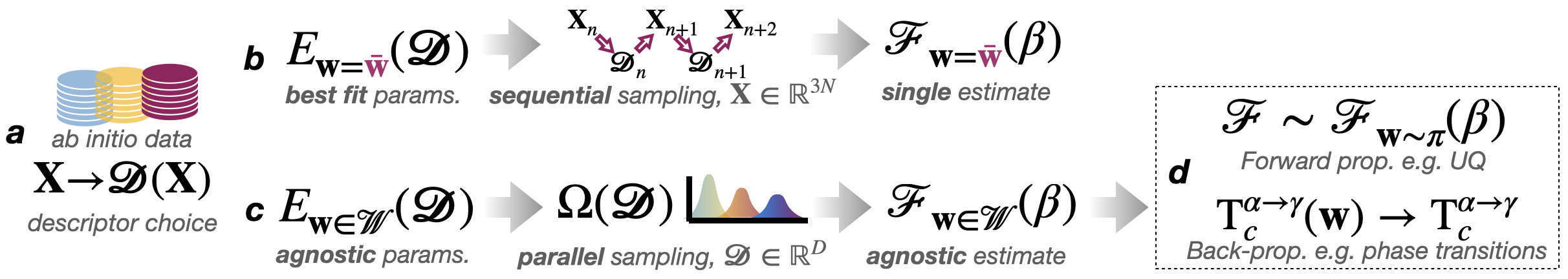
Figure 1: Model agnostic sampling with the descriptor density of states (D-DOS) for uncertainty quantification (UQ) and inverse design. a) Modern atomic simulations choose some set of descriptor functions to represent atomic structure (section III) and build interatomic potentials (MLIPs) that approximate some ab initio dataset. b) Existing approaches determine a single best fit of MLIP parameters then execute sequential Monte Carlo sampling (section II), potentially using descriptors to bias proposalsTamagnone et al. (2024); Ahmad and Cai (2022); Wirnsberger et al. (2022); Noé et al. (2019). The output is a free energy estimate for the specific value of MLIP parameters employed. c) The D-DOS approach instead has agnostic model parameters in some region ${\mathbf{w}}\in\mathcal{W}$, estimating the D-DOS in a parallelized score-matching scheme with around $10\times$ efficiency (section VII). The output is an agnostic estimator which returns free energies and gradients for any parameter value ${\mathbf{w}}\in\mathcal{W}$. d) D-DOS enables rapid UQ in forward propagation and, uniquely, inverse design in back-propagation (section VIII) to fine-tune e.g. phase transition temperatures. In d), $\sim$ indicates ‘distributed as’.

However, all current approaches still require a priori specification of MLIP parameters before any sampling is performed. The restriction to specific model parameters significantly complicates exploration of how MLIP parameters influence finite temperature properties, which has gained increasing interest for both uncertainty quantificationSwinburne and Perez (2025); Imbalzano et al. (2021); Musil et al. (2019); Best et al. (2024); Zhu et al. (2023) in forward-propagation and an array of inverse design goals in back-propagationThaler et al. (2022); Lopanitsyna et al. (2023), such as targeted fine-tuningGrigorev et al. (2023); Maliyov et al. (2025).

In this paper, we propose a completely new approach for model-agnostic sampling, introducing the descriptor density of states (D-DOS) $\Omega({\bm{\mathcal{D}}})$, a generalization of the energy DOS. Our main result is the D-DOS entropy (log density) can be efficiently estimated via score matching to yield an accurate free energy estimator without a priori specification of model parameters. Numerical experiments demonstrate forward propagation for UQ and back propagation for inverse fine-tuning, to our knowledge a first demonstration for free energies and phase boundaries. An overview of the D-DOS approach in relation to existing schemes is illustrated in figure 1.

The paper is structured as follows. After reviewing existing free energy estimation schemes in section II, we discuss descriptor-based MLIPs in section III, where we show how a broad class of MLIPsShapeev (2016); Thompson et al. (2015); Lysogorskiy et al. (2021); Goryaeva et al. (2021a); Nguyen (2023); Batatia et al. (2023); Perez et al. (2025) can be expressed as a linear sum of descriptor features. Section IV then introduces the D-DOS, showing how the exponential divergence of any density of states expressionWang and Landau (2001); Pártay et al. (2021) via a conditional scheme in close analogy to free energy perturbation. While general to any descriptor-based MLIP, in section V we show that for MLIPs linear in descriptor features, the free energy can be exactly expressed as the Legendre-Fenchel conjugate of the descriptor entropy, avoiding high-dimensional integration through Laplace’s method in the limit $N\to\infty$. We show the descriptor entropy has a maximum of zero, meaning we can integrate the entropy gradient estimated via score matchingHyvärinen and Dayan (2005), detailed in section VI.

Our final result is a lightweight, differentiable, model-agnostic estimate that can be employed in forward or back propagation. In section VII, we detail the numerical implementation of reference free energy calculations and our score matching scheme, for which an open source code is providedSwinburne and Marinica (2025). Section VIII presents extensive numerical experiments, demonstrating the ability of our approach to predict solid state free energies for a broad range of models, covering BCC and A15 phases of W and Mo, finding typical errors of 1-2 meV/atom against established free energy estimation schemes. We then provide a first exploration of inverse fine-tuning for free energy curves focusing on the BCC and FCC phases of W and Fe, targeting the $\alpha\to\gamma$ transition temperature.

We discuss the many possible perspectives for our approach in the conclusions (section IX), including inverse design applications and extension to foundational MLIPsBatzner et al. (2022); Batatia et al. (2023); Bochkarev et al. (2024). As our approach allows practical implementation of density of states methodsWang and Landau (2001); Pártay et al. (2021) to very high-dimensional systems, we anticipate application across the many areas of computational science that use linear feature modelsMarchand et al. (2023); Follain and Bach (2024); Ekborg-Tanner et al. (2024).

I Introductory example with the energy density of states

As a guide to the reader, we first illustrate our approach by showing how access to the energy density of states $\Omega(U)$ allows for temperature-agnostic sampling, which this paper generalizes to model-agnostic sampling with $\Omega({\bm{\mathcal{D}}})$, the descriptor density of states (D-DOS). Leaving detailed definitions for later sections, with $\Omega(U)$ the classical partition function at ${\rm T}=1/({\rm k_{B}}\beta)$ writes

$$Z(\beta)=\int_{0}^{\infty}\Omega(U)\exp(-\beta U){\rm d}U.$$ (1)

For systems with local interactions $\Omega(U)$ can be cast in terms of an intensive $\mathcal{S}(u)$ as $N\to\infty$, where $u=U/N$:

$$\Omega(U)\to\Omega_{0}e^{N\mathcal{S}(u)},\quad Z(\beta)\to Z_{0}\int_{0}^{\infty}e^{N(\mathcal{S}(u)-\beta u)}du,$$

with $\Omega_{0},Z_{0}$ constants. $Z(\beta)$ is dominated by the maximum of the integrand as $N\to\infty$, allowing exact free energy evaluation via Laplace’s method (appendix A):

$$\mathcal{F}(\beta)\equiv\lim_{N\to\infty}\frac{-\ln|Z(\beta)|}{\beta N}=\min_{u}u-\mathcal{S}(u)/\beta.$$ (2)

We thus see that access to $\mathcal{S}(u)$ allows temperature agnostic estimation through minimization with $-\beta\mathcal{F}(\beta)$ defined as the Legendre-Fenchel conjugate of $\mathcal{S}(u)$Fenchel (1949). This paper generalizes the above from $\Omega(U)$ to $\Omega({\bm{\mathcal{D}}})$, enabling model-agnostic MLIP sampling.

II Thermodynamic sampling of atomic crystal models

This section reviews standard results from classical statistical mechanics for a system of $N$ atoms with specie ${\bf s}=[{\rm s}_{1},\dots,{\rm s}_{N}]\in\mathbb{Z}^{N}$, positions ${\mathbf{X}}=[{\bf x}_{1},\dots,{\bf x}_{N}]\in\mathbb{R}^{N\times 3}$ and momenta ${\bf P}=[{\bf p}_{1},\dots,{\bf p}_{N}]\in\mathbb{R}^{N\times 3}$. Atoms are confined to a periodic supercell ${\bf C}\in\mathbb{R}^{3\times 3}$ with volume $V=|{\bf C}|$ (the determinant), such that scaled positions lie on the unit torus, i.e. ${\mathbf{X}}{\bf C}^{-1}\in\mathbb{T}^{N\times 3}$. In anticipation of later results where we take the limit $N\to\infty$, we write the total energy $U({\mathbf{X}},{\bf P})$ as the sum of an intensive potential and kinetic energy, i.e.

$$U({\bf X},{\bf P})\equiv N[{E}_{{\mathbf{w}}}({\mathbf{X}})+{K}({\bf P})],$$ (3)

where ${K}({\bf P})=(1/N)\sum_{i=1}^{N}{\rm p}^{2}_{i}/(2m_{i})$ and dependence on ${\bf s}$ is contained in the potential energy function ${E}_{\mathbf{w}}({\mathbf{X}})$ by model parameters ${\mathbf{w}}$, the focus of this paper, treated in section III. To express the supercell in an intensive form we define the supercell per atom ${{\bf c}}$ through ${\bf C}={\bf N}{{\bf c}}$, where ${\bf N}={\rm Diag}(N_{x},N_{y},N_{z})$, such that $|{\bf N}|=N$ and the volume per atom is given by $|{{\bf c}}|$. The canonical (NVT) partition function at ${\rm T}=1/({\rm k_{B}}\beta)$ then writes

$$Z^{N}_{\mathbf{w}}(\beta,{{\bf c}}) \equiv\lambda_{0}(\beta)^{-3N}\int_{\mathbb{R}^{3N}}\exp[-N\beta E_{\mathbf{w}}({\mathbf{X}})]{\rm d}{\mathbf{X}},$$ (4)

where $\lambda_{0}(\beta)=\hbar\sqrt{2\pi\beta/m}$ is the thermal De Broglie wavelengthFrenkel and Smit (1996) and ${m}^{N}\equiv\prod_{i=1}^{N}m_{i}$. The NVT free energy per atom is defined in the thermodynamic limit $N\to\infty$:

$$\mathcal{F}_{\mathbf{w}}(\beta,{{\bf c}})\equiv\lim_{N\to\infty}\frac{-1}{\beta N}\ln|Z^{N}_{\mathbf{w}}(\beta,{{\bf c}})|.$$ (5)

In practice, the integral over atomic configuration space in (4) is dominated by contributions from some set of phases $\mathcal{P}=\{$bcc, fcc, hcp, liquid, $\dots\}$, such that

$$Z^{N}_{\mathbf{w}}(\beta,{{\bf c}})=\sum_{p\in\mathcal{P}}Z^{N}_{\mathbf{w}}(\beta,{{\bf c}},p),$$ (6)

where each term $Z^{N}_{\mathbf{w}}(\beta,{{\bf c}},p)$, is an integral over (disjoint) partitions of configuration space, with corresponding phase free energy $\mathcal{F}_{\mathbf{w}}(\beta,{{\bf c}},p)$, defined as in (5). It is simple to show that as $N\to\infty$ the NVT free energy is dominated by a single phase

$$p_{\mathbf{w}}^{*}(\beta,{{\bf c}})=\arg\min_{p\in\mathcal{P}}\mathcal{F}_{\mathbf{w}}(\beta,{{\bf c}},p),$$ (7)

as $\mathcal{F}_{\mathbf{w}}(\beta,{{\bf c}})=\min_{p\in\mathcal{P}}\mathcal{F}_{\mathbf{w}}(\beta,{{\bf c}},p)$. Similarly, the NPT free energy of a phase $p$ is obtained by minimizing $\mathcal{F}_{\mathbf{w}}(\beta,{{\bf c}},p)$ at under some constant external stress ${\bm{\sigma}}$ (i.e. isotropic pressure ${\bm{\sigma}}=(P/3)\mathbb{I}_{3}$), giving

$$\mathcal{G}_{\mathbf{w}}(\beta,{\bm{\sigma}},p)\equiv\min_{{\bf c}}\mathcal{F}_{\mathbf{w}}(\beta,{{\bf c}},p)-{\rm Tr}({\bm{\sigma}}^{\top}{{\bf c}}),$$ (8)

It is clear that estimation of $\mathcal{F}_{\mathbf{w}}(\beta,{{\bf c}},p)$ for general $\beta,{{\bf c}}$ is sufficient to estimate $\mathcal{G}_{\mathbf{w}}(\beta,{\bm{\sigma}},p)$, giving the stable phase at some temperature and pressure as

$$p^{*}_{\mathbf{w}}(\beta,{\bm{\sigma}})=\arg\min_{p\in\mathcal{P}}\mathcal{G}_{\mathbf{w}}(\beta,{\bm{\sigma}},p),$$ (9)

where the ${\mathbf{w}}$ subscript emphasizes the dependence of $p^{*}$ on the parameters of the interatomic potential.

In this paper, we will focus on the set of crystalline phases $\mathcal{P}_{s}\subset\mathcal{P}$, whose configuration space is defined as the set of (potentially large) vibrations around some lattice structure ${\mathbf{X}}_{p}^{0}$, $p\in\mathcal{P}_{s}$. Extension of the present approach to liquid phases is discussed in IX.

II.1 Thermodynamic integration

Accurate calculation of phase stability requires converging per-atom free energy differences between phases to within a few meV/atom at any given temperature and pressure to allow determination of (9). Accurate determination of phase transitions, where free energy differences are formally zeroZhu et al. (2017); Grabowski et al. (2019); Zhong et al. (2023); Zhu et al. (2024); Menon et al. (2024), thus requires tight convergence of any estimator. The stringent accuracy requirement has led to the development of sampling techniques to reduce the number of samples required for convergence Kirkwood (1935); Frenkel and Smit (1996); Rickman and LeSar (2002). In all cases, the starting point is some atomic energy function $E_{0}({\bf X})$, whose corresponding phase free energy $\mathcal{F}_{0}(\beta,{{\bf c}},p)$ is known either through tabulation, or analytically if $E_{0}({\bf X})$ is harmonicKirkwood (1935). We can thus define $\Delta E_{\mathbf{w}}({\mathbf{X}})=E_{\mathbf{w}}({\mathbf{X}})-E_{0}({\mathbf{X}})$ as the energy difference (per-atom) between the target and reference systems, with a free energy difference $\Delta\mathcal{F}_{\mathbf{w}}(\beta,{{\bf c}},p)$. Thermodynamic integration (TI) is a stratified sampling scheme over $E_{\eta}({\bf X})=E_{0}({\bf X})+\eta\Delta E_{\bf w}({\bf X})$ for $\eta\in[0,1]$. Denoting equilibrium averages by $\langle\dots\rangle_{\eta}$, we obtain

$$\Delta\mathcal{F}_{\bf w}(\beta,{{\bf c}},p) =\int_{0}^{1}\langle\Delta E_{\bf w}({\bf X})\rangle_{\eta}\,{\rm d}\eta.$$ (10)

Sampling efficiency often requires constraint functions or resetting to prevent trajectories escaping the metastable basin of a given phase, as discussed in section VII.4. In general, the larger the value of $\Delta\mathcal{F}_{\bf w}$, the finer the integration scheme over $\eta$ and the more samples will be required for convergence Lelièvre et al. (2010); Comer et al. (2015).

II.2 Free energy perturbation

Typically used as a complement to thermodynamic integration, if the difference $N\Delta E_{\mathbf{w}}({\mathbf{X}})$ is as small as $10/\beta$, corresponding to at most 10 meV/atom at 1000 K for solid state systems ($N\simeq 100$), we can also use free energy perturbation (FEP) to estimate the free energy differenceLelièvre et al. (2010); Grabowski et al. (2019); Castellano et al. (2022). Using the definition of the free energy $\mathcal{F}_{\mathbf{w}}(\beta,{{\bf c}})$ and $\langle\dots\rangle_{\eta}$ at $\eta=0$, it is simple to show that

$$\Delta\mathcal{F}_{\bf w}(\beta,{{\bf c}},p) =-(1/N\beta)\ln\langle\exp[-N\beta\Delta E_{\bf w}({\mathbf{X}})]\rangle_{0}.$$

In practice, the logarithmic expectation is expressed as a cumulant expansionZwanzig (1954); Lelièvre et al. (2010); Castellano et al. (2024) for increased numerical stability, writing

$$\Delta\mathcal{F}_{\bf w}(\beta,{{\bf c}},p)=\langle{\Delta E_{\bf w}}\rangle_{0}-\frac{N\beta}{2}\langle(\delta\Delta E_{\bf w})^{2}\rangle_{0}+\dots,$$ (11)

where $\delta\Delta E_{\bf w}=\Delta E_{\bf w}-\langle{\Delta E_{\bf w}}\rangle_{0}$, and the expansion continues, in principle, to all orders. While (11) gives an expression for the free energy in terms of samples generated solely with a reference potential, in a practical setting we require free energy differences to be very small to allow for convergence. Equation (11) can be shown to be an upper bound to the estimated free energy differenceCastellano et al. (2022) and as such can be used as a convergence measure for a well-chosen reference potential. In this setting, we typically have $\Delta\mathcal{F}_{\bf w}<1$ meV/atom (table 1).

II.3 Adiabatic Switching

In addition to the above methods which employ equilibrium averages, the adiabatic switchingAdjanor et al. (2006); de Koning et al. (1999); Freitas et al. (2016); Menon et al. (2024) method estimates free energy differences using the well-known Jarzynski equality Jarzynski (1997). The adiabatic switching equality can be writtenFreitas et al. (2016)

$$\Delta\mathcal{F}_{\bf w}(\beta,{{\bf c}},p) =\frac{1}{2}[\langle W^{\textrm{irr}}\rangle_{0\to 1}-\langle W^{\textrm{irr}}\rangle_{1\to 0}],$$ (12)

where $W^{\textrm{irr}}$ is the irreversible work along a thermodynamic path (in the above $\eta$ is implied, though it is also possible to use the temperature) and $\langle\dots\rangle_{0\to 1}$ indicates an ensemble average of around $10-30$ simulations. The key quantity is the so-called ‘switching time’, i.e. the rate at which the thermodynamic path is traversed. For solid-state free energies one typically progresses along the path in $\mathcal{O}(10)$ increments of $\mathcal{O}(10-100)$ psMenon et al. (2024), thus requiring around $10^{7-8}$ force calls per temperature. In this setting, we can target similar free energy differences to thermodynamic integration, i.e. $\mathcal{O}(100)$ meV/atom at 1000 K. The computational costs of the above methods and the present D-DOS approach is discussed in section VII, and summarized in table 1.

III Descriptor-based interatomic potentials

The search for efficient and accurate interatomic potentials is a central goal of computational materials scienceDeringer et al. (2019). For systems without long-range interactions, the intensive energy in (3) is modeled as a sum of functions over local atomic environments

$$E_{\mathbf{w}}({\mathbf{X}})=\frac{1}{N}\sum_{i=1}^{N}E^{1}_{\mathbf{w}}({\bf R}_{i},{\bf s}_{i}),$$ (13)

where ${\bf R}_{i}=[\dots,{\bf r}_{ij},\dots]$ is a set of vectors from $i$ to all neighbors $j$ within some cutoff $r_{c}$, ${\bf s}_{i}=[\dots,{\rm s}_{j},\dots]$ are the corresponding chemical species (along with ${\rm s}_{i}$ of $i$) and ${\mathbf{w}}$ are learnable model parameters. Modern interatomic potentials typically represent local atomic environments through scalar-valued and dimensionless (i.e. unit-free) descriptor vectors

$${\mathbf{D}}_{i}\equiv\hat{{\mathbf{D}}}({\bf R}_{i},{\bf s}_{i},{\bf h})\in\mathbb{R}^{d}$$ (14)

where ${\bf h}\in\mathbb{R}^{H}$ are a set of hyperparameters for encoding atomic species and all adjustable parameters in $\hat{{\mathbf{D}}}$, and $d$ is the descriptor dimension. A general descriptor-based interatomic potential then has total energy

$$E_{\mathbf{w}}({\mathbf{D}}_{1},\dots,{\mathbf{D}}_{N})=\frac{1}{N}\sum_{i=1}^{N}E^{1}_{\mathbf{w}}({\mathbf{D}}_{i}),$$ (15)

where we suppress the chemical vectors ${\bf s}_{i}$ as they are considered encoded in the ${\mathbf{D}}_{i}$. For systems with $M$ atomic species $d$ formally increases combinatorially with $M$, but in practice sparsification schemes give $d=\mathcal{O}(M)$Darby et al. (2023); Thompson et al. (2015). In this work, we consider potentials of the general linear form, with parameters ${\mathbf{w}}\in\mathbb{R}^{D}$,

$$E^{L}_{\mathbf{w}}({\bm{\mathcal{D}}})\equiv{\mathbf{w}}^{\top}{\bm{\mathcal{D}}},\quad{\bm{\mathcal{D}}}\equiv\frac{1}{N}\sum_{i=1}^{N}\hat{{\bm{\phi}}}({\mathbf{D}}_{i})\in\mathbb{R}^{D},$$ (16)

where $\hat{{\bm{\phi}}}({\mathbf{D}}_{i})=[\hat{\phi}_{1}({\mathbf{D}}_{i}),\dots,\hat{\phi}_{D}({\mathbf{D}}_{i})]$ is a $D$-dimensional featurization of ${\mathbf{D}}_{i}\in\mathbb{R}^{d}$ and the $L$ superscript denotes the linear form. Importantly, ${\bm{\mathcal{D}}}$ is independent of parameters ${\mathbf{w}}$, and the dimension $D$ is typically larger than $d$ but intensive, i.e. independent of $N$, which is required to apply Laplace’s method in section V.

III.1 Admissible interatomic potentials

A wide variety of interatomic potentials can be cast into the general linear form (16). Clearly, these include the broad class of linear-in-descriptor (LML) models, including MTPShapeev (2016), ACFS Behler (2011, 2016), SNAPThompson et al. (2015), SOAP Bartók et al. (2013); Darby et al. (2022, 2023), ACEDrautz (2019, 2020); Lysogorskiy et al. (2021), MILADYGoryaeva et al. (2021a); Dézaphie et al. (2025) and PODNguyen (2023) descriptors, where

$$\hat{{\bm{\phi}}}_{\tt{LML}}({\mathbf{D}}_{i})={\mathbf{D}}_{i}\in\mathbb{R}^{d}.$$ (17)

LML models can reach extremely high ($<2$ meV/atom) accuracy to ab initio dataCastellano et al. (2024), with robust UQSwinburne and Perez (2025) and often excellent dynamical stability, essential for thermodynamic samplingZhu et al. (2017); Grabowski et al. (2019); Zhong et al. (2023); Zhu et al. (2024); Menon et al. (2024). Polynomial or kernel featurizations are regularly used to increase flexibility, e.g. qSNAPRohskopf et al. (2023), PiPAllen et al. (2021) GAPBartók and Csányi (2015); Deringer et al. (2019), n-body kernels Glielmo et al. (2017, 2018); Vandermause et al. (2020); Xie et al. (2021), kernelZhong et al. (2023) etc. For example, with qSNAP we have the quadratic featurization

$$\hat{{\bm{\phi}}}_{\tt{qSNAP}}({\mathbf{D}}_{i})={\mathbf{D}}_{i}\oplus{\tt{vech}}({\mathbf{D}}_{i}\otimes{\mathbf{D}}_{i})\in\mathbb{R}^{d(d+3)/2},$$ (18)

i.e. $D=d(d+3)/2$ as ${\tt{vech}}({\mathbf{D}}_{i}\otimes{\mathbf{D}}_{i})\in\mathbb{R}^{d(d+1)/2}$ returns a vector from the quadratic product ${\mathbf{D}}_{i}\otimes{\mathbf{D}}_{i}\in\mathbb{R}^{d\times d}$.

The generalized linear form can encompass more complex models if we only consider a subset of parameters adjustable, an approach adopted when fine-tuning recent message-passing neural network (MPNN) modelsBatzner et al. (2022); Musaelian et al. (2023); Batatia et al. (2022, 2023); Bochkarev et al. (2024); Cheng (2024); Batatia et al. (2025). In this case, we consider inputs of the MPNN readout layer $h({\mathbf{D}}_{i})$ as descriptors ${\mathbf{D}}_{i}$, then express the readout layer as a general linear model of the desired form (16). For example, in the MACE MPNN architectureBatatia et al. (2022), the readout layer is a sum of a linear function and a one layer neural network $f({\mathbf{D}}_{i})$, giving the featurization

$$\hat{{\bm{\phi}}}_{\tt{MACE}}({\mathbf{D}}_{i})={\mathbf{D}}_{i}\oplus f({\mathbf{D}}_{i})\in\mathbb{R}^{d+1},$$ (19)

i.e. $D=d+1$ as we treat the neural network as a fixed feature function, such that adjustable parameters ${\mathbf{w}}$ cover all linear-in-descriptor terms and a scalar prefactor on the neural network. Recent work has shown this allows uncertainty quantification schemes for linear modelsSwinburne and Perez (2025) to be applied to the MACE-MPA-0 foundation modelBatatia et al. (2023), successfully bounding prediction errors across the materials project databasePerez et al. (2025). More generally, one could also aim to learn a set of descriptor feature functions $\hat{{\bm{\phi}}}({\mathbf{D}}_{i})$ and a set of parameter feature functions $\hat{{\bm{\psi}}}({\mathbf{w}})$ to minimize the loss $L({\bm{\Theta}})=\sum_{i}\|\hat{{\bm{\psi}}}({\mathbf{w}})^{\top}\hat{{\bm{\phi}}}({\mathbf{D}}_{i})-E_{\mathbf{w}}({\mathbf{D}}_{i})\|^{2}$ to some $E_{\mathbf{w}}({\mathbf{D}}_{i})$, giving a generalized linear feature model under ${\mathbf{w}}\to\hat{{\bm{\psi}}}({\mathbf{w}})$, a direction we leave for future research. As a result, while the numerical applications of this paper (section VII) focus on linear MLIPs with SNAP descriptors, i.e. equation (17), the D-DOS approach opens many broader perspectives which are discussed further in section IX.

IV The descriptor density of states

The NVT free energy is defined in equation (5). Suppressing dependence on $p$ and ${{\bf c}}$ for clarity, the free energy for the generalized linear MLIPs (16) can be written

$$\mathcal{F}^{L}_{\mathbf{w}}(\beta)=\lim_{N\to\infty}\frac{-1}{N\beta}\ln\left|\lambda_{0}^{-3N}(\beta)\int_{\mathbb{R}^{D}}e^{-N\beta{\mathbf{w}}\cdot{\bm{\mathcal{D}}}}\Omega({\bm{\mathcal{D}}}){\rm d}{\bm{\mathcal{D}}}\right|,$$

where $\Omega({\bm{\mathcal{D}}})$ is the descriptor density of states (D-DOS)

$$\Omega({\bm{\mathcal{D}}})\equiv\int_{\mathbb{R}^{3N}}\delta\left({\bm{\mathcal{D}}}-\sum_{i=1}^{N}\hat{{\bm{\phi}}}({\mathbf{D}}_{i}({\bf X}))/N\right){\rm d}{\mathbf{X}}.$$ (20)

Estimation of $\Omega({\bm{\mathcal{D}}})$ would allow prediction of $\mathcal{F}_{\mathbf{w}}(\beta)$ for any value of the potential parameters ${\mathbf{w}}$, our central goal. However, this requires overcoming two significant numerical issues. First, $\Omega({\bm{\mathcal{D}}})$ is ill-conditioned, with an integral that grows exponentially with $N$:

$$\int_{\mathbb{R}^{D}}\Omega({\bm{\mathcal{D}}}){\rm d}{\bm{\mathcal{D}}}=V^{N}.$$ (21)

This divergence is common to all density of states, e.g. $\int_{\mathbb{R}}\Omega(E){\rm d}E=V^{N}$, and severely limits the application of Wang-LandauWang and Landau (2001) or nested samplingPártay et al. (2021) at large $N$. Secondly, the global feature vector ${\bm{\mathcal{D}}}\in\mathbb{R}^{D}$ has a very high dimension, typically $\mathcal{O}(100-1000)$ and thus (21) cannot be integrated through direct quadrature, while Monte Carlo estimation is generally slow to converge and cannot give reliable gradient information. The central contributions of this paper are strategies to overcome these two issues. Section IV.1 contains the $V^{N}$ divergence via a conditional scheme, and section V shows how Laplace’s method (appendix A) allows us to avoid high-dimensional integration.

IV.1 The conditional descriptor density of states

To control the $V^{N}$ divergence of $\Omega({\bm{\mathcal{D}}})$, we introduce the conditional descriptor density of states (CD-DOS)

$$\Omega({\bm{\mathcal{D}}}|\alpha)\equiv \int_{\mathbb{R}^{3N}}\frac{\delta\left(\hat{\alpha}({\mathbf{X}})-\alpha\right)}{\Omega(\alpha)}$$

$$\times\delta\left({\bm{\mathcal{D}}}-\sum_{i=1}^{N}\hat{{\bm{\phi}}}({\mathbf{D}}_{i}({\bf X}))/N\right){\rm d}{\mathbf{X}},$$ (22)

where $\hat{\alpha}({\mathbf{X}})$ is the dimensionless function

$$\hat{\alpha}({\mathbf{X}})\equiv\ln\left|{{E}_{0}({\bf X})}/{\rm U}_{0}\right|,$$ (23)

${\rm U}_{0}$ is a user-defined energy scale and ${E}_{0}({\bf X})\geq 0$ is some intensive reference potential energy, as in equation (3). In section IV.3 we detail how equation (23) can be generalized to a momentum-dependent $\hat{\alpha}({\mathbf{X}},{\bf P})$. In either case, ${E}_{0}({\bf X})$ is chosen such that we can calculate, numerically or analytically, the isosurface volume

$$\Omega(\alpha)\equiv\int_{\mathbb{R}^{3N}}\delta\left(\hat{\alpha}({\mathbf{X}})-\alpha\right){\rm d}{\bf X},$$ (24)

which contains the exponential divergence as $\int_{\mathbb{R}}\Omega(\alpha){\rm d}\alpha=V^{N}$. The crucial advantage of this conditional form is that estimation of $\Omega({\bm{\mathcal{D}}}|\alpha)$ is then much simpler, as it is normalized by construction:

$$\int_{\mathbb{R}^{D}}\Omega({\bm{\mathcal{D}}}|\alpha){\rm d}{\bm{\mathcal{D}}}=\frac{\Omega(\alpha)}{\Omega(\alpha)}=1.$$ (25)

This normalization allows us to employ density estimation techniques such as score matchingHyvärinen and Dayan (2005). Equation (25) shows $\Omega({\bm{\mathcal{D}}}|\alpha)$ is the probability density function of ${\bm{\mathcal{D}}}$ on the isosurface $\hat{\alpha}({\mathbf{X}})=\alpha$. The full D-DOS $\Omega({\bm{\mathcal{D}}})$ is then formally recovered through integration against $\alpha$:

$$\Omega({\bm{\mathcal{D}}})=\int_{\mathbb{R}}\Omega({\bm{\mathcal{D}}}|\alpha)\Omega(\alpha){\rm d}\alpha.$$ (26)

Equation (26) emphasizes that our goal is to decompose the high-dimensional configuration space into a foliation of isosurfaces $\hat{\alpha}({\mathbf{X}})=\alpha$ where we expect $\Omega({\bm{\mathcal{D}}}|\alpha)$ to be tractable for density estimation. The generalization of $\hat{\alpha}({\mathbf{X}})$ to include momentum dependence is discussed in section IV.3 and general considerations for designing optimal $\hat{\alpha}({\mathbf{X}})$ are discussed in section V.3

IV.2 The isosurface and descriptor entropies

The free energy $\mathcal{F}_{\mathbf{w}}(\beta)$, equation (5), is proportional to the intensive logarithm of the partition function $Z_{\mathbf{w}}(\beta)$, i.e. $\mathcal{F}_{\mathbf{w}}(\beta)=(-1/N\beta)\ln|Z_{\mathbf{w}}(\beta)|$. To estimate free energies, it is thus natural to define intensive entropies of the isosurface volume $\Omega(\alpha)$ and CD-DOS $\Omega({\bm{\mathcal{D}}}|\alpha)$. As we use $\beta=1/({\rm k_{B}T})$ rather than $\rm T$, we omit factors of ${\rm k_{B}}$ such that entropies are dimensionless.

We first define the intensive isosurface entropy

$$\mathcal{S}_{0}(\alpha)\equiv\lim_{N\to\infty}\frac{1}{N}\ln|\Omega(\alpha)/V^{N}_{0}|.$$ (27)

The term $V_{0}$ ensures $\mathcal{S}_{0}(\alpha)$ is dimensionless; with $\hat{\alpha}({\mathbf{X}})$ we have $V_{0}=\lambda^{3}_{0}(\beta)$, while with a momentum-dependent $\hat{\alpha}({\mathbf{X}},{\bf P})$, discussed in IV.3, we have $V_{0}=h^{3}$. It is clear that $\mathcal{S}_{0}(\alpha)$ is a measure of the configurational entropy per atom of $N$ independent atoms confined to the isosurface. The CD-DOS $\Omega({\bm{\mathcal{D}}}|\alpha)$, equation (22), has a natural entropy definition, the intensive log density

$$\mathcal{S}({{\bm{\mathcal{D}}}}|\alpha)\equiv\lim_{N\to\infty}\frac{1}{N}\ln\Omega({{\bm{\mathcal{D}}}}|\alpha).$$ (28)

The CD-DOS entropy $\mathcal{S}({\bm{\mathcal{D}}}|\alpha)$ measures the proportion of the isosurface phase space volume that has a global descriptor vector ${\bm{\mathcal{D}}}$, meaning descriptor values with larger $\mathcal{S}({{\bm{\mathcal{D}}}}|\alpha)$ are more likely to be observed under unbiased isosurface sampling. Furthermore, $\mathcal{S}({{\bm{\mathcal{D}}}}|\alpha)$ has two properties which greatly facilitate free energy estimation. In appendix D, we show that as the per-atom descriptor features ${\bm{\phi}}({\mathbf{D}}_{i})\in\mathbb{R}^{D}$ depend only on the local environment of atom $i$, the CD-DOS entropy $\mathcal{S}({{\bm{\mathcal{D}}}}|\alpha)$ is intensive ($N$-independent). Secondly, as $\Omega({\bm{\mathcal{D}}}|\alpha)$ is normalized, application of Laplace’s method (appendix A) gives a very useful result that fixes the maximum of $\mathcal{S}({{\bm{\mathcal{D}}}}|\alpha)$:

$$\lim_{N\to\infty}\frac{1}{N}\ln\left|\int\Omega({{\bm{\mathcal{D}}}}|\alpha){\rm d}{\bm{\mathcal{D}}}\right|=\max_{{\bm{\mathcal{D}}}\in\mathbb{R}^{D}}\mathcal{S}({{\bm{\mathcal{D}}}}|\alpha)=0.$$ (29)

In section V we show that free energy estimation for linear‐in‐descriptor MLIPs reduces to a minimization over $\mathbf{w}^{\top}{\bm{\mathcal{D}}}-\beta^{-1}[\mathcal{S}({\bm{\mathcal{D}}}|\alpha)+\mathcal{S}_{0}(\alpha)]$, avoiding high-dimensional integration. Moreover, section VI shows $\mathcal{S}({\bm{\mathcal{D}}}|\alpha)$ can be approximated through score matching of $\nabla_{{\bm{\mathcal{D}}}}\mathcal{S}({\bm{\mathcal{D}}}|\alpha)$, where (29) fixes the subsequent constant of integration to give an absolute estimate of $\mathcal{S}({{\bm{\mathcal{D}}}}|\alpha)$.

IV.3 Forms of the isosurface function

As discussed above, free energy estimation will require access to $\mathcal{S}_{0}(\alpha)$ and a means to generate samples on the isosurface $\hat{\alpha}({\mathbf{X}})=\alpha$. For harmonic reference potentials $S_{0}(\alpha)$ is given analytically; the isosurface function writes

$$\hat{\alpha}({\mathbf{X}})\equiv\ln\left|{[{\mathbf{X}}-{\mathbf{X}}_{0}]^{\top}{\bf H}[{\mathbf{X}}-{\mathbf{X}}_{0}]}/({2N\rm U_{0}})\right|,$$ (30)

where the Hessian ${\bf H}$ has 3$N$-3 positive eigenmodes and ${\mathbf{X}}_{0}$ is the lattice structure. As detailed in appendix B, sampling $\hat{\alpha}({\bf X})=\alpha$ reduces to generating random unit vectors in $\mathbb{R}^{3N-3}$, while the isosurface entropy (27) reads

$$\mathcal{S}_{0}(\alpha)\equiv S_{0}+3\alpha/2,\quad V_{0}=\lambda^{3}_{0}(\beta).$$ (31)

In appendix B, we show the constant $S_{0}$ is given by $S_{0}=3/2+3/2\ln|2\beta{\rm U}_{0}/3|-\beta\mathcal{F}_{0}(\beta)$, where $\mathcal{F}_{0}(\beta)$ is the familiar free energy per-atom of an atomic system governed by the harmonic potential $E_{0}({\mathbf{X}})$.

To go beyond harmonic reference models to arbitrary $E_{0}({\mathbf{X}})$, we generalize (23) to accommodate the intensive kinetic energy ${K}({\bf P})=(1/N)\sum_{i=1}^{N}{\rm p}^{2}_{i}/(2m_{i})$ from (3), such that the isosurface value is the log total energy

$$\hat{\alpha}({\mathbf{X}},{\bf P})\equiv\ln\left|[{K}({\bf P})+E_{0}({\bf X})]/{\rm U}_{0}\right|.$$ (32)

Isosurface sampling then reduces to running microcanonical (NVE) dynamics, in close connection with Hamiltonian Monte CarloBetancourt (2017); Livingstone et al. (2019). In appendix C, we show the NVT free energy $\mathcal{F}_{0}(\beta)$ of the reference system can be expressed as $\mathcal{F}_{0}(\beta)=\mathcal{U}_{0}(\beta)-\mathcal{S}_{0}(\alpha_{\beta})$, where $\mathcal{U}_{0}(\beta)$ is the internal energy per atom and $\alpha_{\beta}\equiv\ln|\mathcal{U}_{0}(\beta)/{\rm U}_{0}|$.
As a result, with a momentum-dependent isosurface (32) the isosurface entropy (27) is simply the difference between the reference system’s free and internal energies:

$$\mathcal{S}_{0}(\alpha)=\beta_{\alpha}\left[\mathcal{U}_{0}(\beta_{\alpha})-\mathcal{F}_{0}(\beta_{\alpha})\right],\quad V_{0}(\alpha)=h^{3},$$ (33)

where $\beta_{\alpha}$ is defined through $\mathcal{U}_{0}(\beta_{\alpha})\equiv{\rm U}_{0}\exp(\alpha)$, which will have a unique solution when $\mathcal{U}_{0}(\beta_{\alpha})$ is monotonic. In practice, the internal and free energies $\mathcal{U}_{0}(\beta)$ and $\mathcal{F}_{0}(\beta)$ are estimated via thermodynamic sampling (II) over a range of $\beta$, interpolating with $\alpha\equiv\ln|\mathcal{U}_{0}(\beta)/{\rm U}_{0}|$ to estimate $\mathcal{S}_{0}(\alpha)$.
The final modification, detailed in appendix C, is to augment the descriptor vector ${\bm{\mathcal{D}}}$, concatenating the kinetic energy as a scalar momentum descriptor $K={K}({\bf P})$

$${\bm{\mathcal{D}}}\to{\bm{\mathcal{D}}}\oplus K,\quad{\mathbf{w}}\to{\mathbf{w}}\oplus 1,$$ (34)

meaning ${\mathbf{w}}^{\top}{\bm{\mathcal{D}}}$ now returns the total energy rather than the potential energy.

In conclusion, sampling schemes can thus use $\hat{\alpha}({\mathbf{X}})$ with a harmonic reference potential, where $\mathcal{S}_{0}(\alpha)$ is given analytically, or $\hat{\alpha}({\mathbf{X}},{\bf P})$ with any reference potential, where $\mathcal{S}_{0}(\alpha)$ determined via thermodynamic sampling. All theoretical results below can use either $\mathcal{S}_{0}(\alpha)$; use of both are demonstrated for solid phases in section VIII.2. A forthcoming study will apply the momentum-dependent formalism to liquid phases and melting transitions. temperature prediction.

V Free energy evaluation with Laplace’s method

Laplace’s method, or steepest descentsWong (2001), is a common technique for evaluating the limiting form of integrals of exponential functions. Consider a twice differentiable function $f({\bf x}):\mathbb{R}^{p}\to\mathbb{R}$ that has a unique minimum in $\mathbb{R}^{p}$ and is intensive, i.e. independent of $N$. Under some mild technical conditions, discussed in appendix A, Laplace’s method implies the limit

$$\lim_{N\to\infty}\frac{-1}{N}\ln\int_{\mathbb{R}^{p}}\exp[-Nf({\bf x})]{\rm d}{\bf x}=\min_{{\bf x}\in\mathbb{R}^{p}}f({\bf x}).$$ (35)

Application of (35) with $p=D$ and $p=1$ for integrals over ${\bm{\mathcal{D}}}$ and $\alpha$ is our primary device to avoid integration in free energy estimation. Using the definition of the CD-DOS entropy $\mathcal{S}({{\bm{\mathcal{D}}}}|\alpha)$, equation (28), shown to be intensive in appendix D, application of (35) implies that

$$\mathcal{F}^{L}_{{\mathbf{w}}}(\beta|\alpha) \equiv\lim_{N\to\infty}\frac{-1}{N\beta}\ln\left|\int_{\mathbb{R}^{D}}e^{-N\beta{\mathbf{w}}^{\top}{\bm{\mathcal{D}}}}\Omega({\bm{\mathcal{D}}}|\alpha){\rm d}{\bm{\mathcal{D}}}\right|,$$

$$=\min_{{\bm{\mathcal{D}}}\in\mathbb{R}^{D}}\left({\mathbf{w}}^{\top}{\bm{\mathcal{D}}}-\mathcal{S}({{\bm{\mathcal{D}}}}|\alpha)/\beta\right),$$ (36)

meaning $-\beta\mathcal{F}^{L}_{{\mathbf{w}}}(\beta|\alpha)$ is the Legendre–Fenchel Fenchel (1949) conjugate of the entropy $\mathcal{S}({{\bm{\mathcal{D}}}}|\alpha)$ for linear MLIPs. It is clear that the conditional free energy (36) has a close connection to the cumulant expansion in free energy perturbation Castellano et al. (2024), equation (11), a point we discuss further in section V.2. We thus obtain a final free energy expression

$$\mathcal{F}^{L}_{{\mathbf{w}}}(\beta) \equiv\lim_{N\to\infty}\frac{-1}{N\beta}\ln\int_{\mathbb{R}}e^{N[\mathcal{S}_{0}(\alpha)-\beta\mathcal{F}_{{\mathbf{w}}}(\beta|\alpha)]}{\rm d}\alpha,$$

$$=\min_{\alpha\in\mathbb{R}}\left(\mathcal{F}^{L}_{{\mathbf{w}}}(\beta|\alpha)-\mathcal{S}_{0}(\alpha)/\beta\right),$$ (37)

The free energy can also be written as the joint minimization, equivalent to a Legendre–Fenchel transformation when $\mathcal{S}_{0}(\alpha)$ is linear in $\alpha$,

$$\mathcal{F}^{L}_{{\mathbf{w}}}(\beta)=\min_{\alpha,{\bm{\mathcal{D}}}}\left({\mathbf{w}}^{\top}{\bm{\mathcal{D}}}-[\mathcal{S}({{\bm{\mathcal{D}}}}|\alpha)+\mathcal{S}_{0}(\alpha)]/\beta\right).$$ (38)

Equation (38) is our main result, an integration-free expression for the free energy for generalized linear MLIPs (16). The minimization over $\alpha$ and ${\bm{\mathcal{D}}}$ requires

$$\nabla_{\bm{\mathcal{D}}}\mathcal{S}({{\bm{\mathcal{D}}}}|\alpha)=\beta{\mathbf{w}},\quad\partial_{\alpha}\mathcal{F}^{L}_{{\mathbf{w}}}(\beta|\alpha)=\partial_{\alpha}\mathcal{S}_{0}(\alpha)$$ (39)

which emphasizes the Legendre duality between $\beta{\mathbf{w}}$ and ${\bm{\mathcal{D}}}$. Use of a harmonic reference energy (30) gives $\mathcal{S}_{0}(\alpha)=S_{0}+3\alpha/2$, equation (31), as detailed in appendix B, meaning $\partial_{\alpha}\mathcal{S}_{0}(\alpha)=3/2$. Appendix B also recovers familiar results for harmonic models; equation (39) reduces to the equipartition relation $\beta\langle E_{0}\rangle=3/2$.

V.1 Gradients of the free energy

The definition of the free energy (37) as a double minimization over $\alpha$ and ${{\bm{\mathcal{D}}}}$ significantly simplifies the gradient of the free energy with respect to potential parameters ${\mathbf{w}}$ or thermodynamic variables such as temperature $1/\beta$. In particular, access to the gradient with respect to ${\mathbf{w}}$ allows the inclusion of finite temperature properties in objective functions for inverse design goals, a feature we explore in the numerical experiments.

With minimizing values $\alpha^{*}_{\beta,{\mathbf{w}}}$, ${\bm{\mathcal{D}}}^{*}_{\beta,{\mathbf{w}},\alpha^{*}}$ for the isosurface and global descriptor, the ${\mathbf{w}}$-gradient is simply

$$\nabla_{\mathbf{w}}\mathcal{F}^{L}_{{\mathbf{w}}}(\beta) ={\bm{\mathcal{D}}}^{*}_{\beta,{\mathbf{w}},\alpha^{*}}\in\mathbb{R}^{D}.$$ (40)

The internal energy is also a simple expression involving the minimizing vector ${\bm{\mathcal{D}}}^{*}_{\beta,{\mathbf{w}},\alpha^{*}}$; when using $\hat{\alpha}({\mathbf{X}})$, defined in equation (30), we have

$$\mathcal{U}^{L}_{{\mathbf{w}}}(\beta) =\partial_{\beta}(\beta\mathcal{F}^{L}_{{\mathbf{w}}}(\beta))=\frac{3}{2\beta}+{\mathbf{w}}^{\top}{\bm{\mathcal{D}}}^{*}_{\beta,{\mathbf{w}},\alpha^{*}},$$ (41)

while when using $\hat{\alpha}({\mathbf{X}},{\bf P})$, defined in equation (32), the internal energy is simply $\mathcal{U}^{L}_{{\mathbf{w}}}(\beta)={\mathbf{w}}^{\top}{\bm{\mathcal{D}}}^{*}_{\beta,{\mathbf{w}},\alpha^{*}}$. Evaluation of higher order gradients requires implicit derivativesBlondel et al. (2022); Maliyov et al. (2025), e.g. $\partial_{\alpha}{\bm{\mathcal{D}}}^{*}_{\beta,{\mathbf{w}},\alpha^{*}}\in\mathbb{R}^{D}$, $\partial_{\beta}\alpha^{*}\in\mathbb{R}$ or $\partial_{\mathbf{w}}[{\bm{\mathcal{D}}}^{*}_{\beta,{\mathbf{w}},\alpha^{*}}]^{\top}\in\mathbb{R}^{D\times D}$.

When using $\hat{\alpha}({\mathbf{X}})$ the specific heat at constant volume writes, in units of ${\rm k_{B}}$,

$${C^{L}_{V}}=3+\beta^{2}\left[\partial_{\beta}{\bm{\mathcal{D}}}^{*}_{\beta,{\mathbf{w}},\alpha^{*}}+\partial_{\beta}\alpha^{*}_{\beta,{\mathbf{w}}}\partial_{\alpha}{\bm{\mathcal{D}}}^{*}_{\beta,{\mathbf{w}},\alpha^{*}}\right]{\mathbf{w}}.$$ (42)

Further exploration of finite temperature properties through thermodynamic relations, such as thermal expansion, will be the focus of future work.

V.2 Connection to free energy perturbation

The conditional free energy $\mathcal{F}_{{\mathbf{w}}}^{L}(\beta|\alpha)$ can be given by a cumulant expansion, using $\langle\dots\rangle_{\alpha}$ for isosurface averages

$$\mathcal{F}^{L}_{{\mathbf{w}}}(\beta|\alpha)=\langle{\mathbf{w}}^{\top}{\bm{\mathcal{D}}}\rangle_{\alpha}+\frac{N\beta}{2}\langle({\mathbf{w}}^{\top}\delta{\bm{\mathcal{D}}})^{2}\rangle_{\alpha}+\dots$$ (43)

where $\delta{\bm{\mathcal{D}}}={\bm{\mathcal{D}}}-\langle{\bm{\mathcal{D}}}\rangle$. The factor of $N$ to ensures intensivity of the covariance, as discussed in appendix D. Free energy perturbation (FEP)Zwanzig (1954); Lelièvre et al. (2010); Castellano et al. (2024), equation (11) also expresses the free energy difference as a cumulant expansion over canonical averages with $E_{0}({\mathbf{X}})$. As discussed in IV.3, as $N\to\infty$ canonical sampling at $\beta$ is equivalent to isosurface sampling at $\alpha=\alpha_{\beta}$, where the relation between $\beta$ and $\alpha_{\beta}$ depends on the form of the isosurface function $\hat{\alpha}({\mathbf{X}})$ or $\hat{\alpha}({\mathbf{X}},{\bf P})$, e.g. (30) or (32). The FEP estimate is thus equivalent to a D-DOS estimate where we fix ${\alpha}=\alpha_{\beta}$, instead of minimizing over $\alpha$ as in equation (37). When the free energy difference is very small, i.e. the target is very similar to the reference, $\hat{\alpha}=\alpha_{\beta}$ may be a good approximate minimization. However, in the general case it is clear the D-DOS estimate can strongly differ from FEP estimates. This is evidenced later in Figures 3b) and 3c), where the minimizing $\alpha$ value at constant $\beta$ varies strongly with ${\mathbf{w}}$, even at relatively low homologous temperatures (1000 K in W, around 1/4 of the melting temperature), while FEP would predict $\alpha$ to be constant with $\beta$.

V.3 Errors in estimation via Laplace’s method

Estimation of free energies via (37) clearly relies on our ability to accurately approximate the conditional descriptor entropy function $\mathcal{S}({{\bm{\mathcal{D}}}}|\alpha)$ by some estimator, which here will be achieved by score matching in section VI. In this context, the curvature of $\mathcal{S}({{\bm{\mathcal{D}}}}|\alpha)$ in ${\bm{\mathcal{D}}}$ and $\alpha$ is crucial, both for the statistical efficiency of score matching and applicability of Laplace’s method (appendix A). In general, as might be expected, the prediction accuracy and statistical efficiency of any estimator will improve as the curvature increases in magnitude. In close connection with existing free energy estimation schemes, selection of the reference energy function $E_{0}({\mathbf{X}})$ used to build $\hat{\alpha}({\mathbf{X}})$ or $\hat{\alpha}({\mathbf{X}},{\bf P})$ has a strong influence on the curvature of $\mathcal{S}({{\bm{\mathcal{D}}}}|\alpha)$ and thus any estimate $\mathcal{S}_{\bm{\Theta}}({{\bm{\mathcal{D}}}|\alpha})$. A poorly chosen reference function will result in weaker curvature, as the descriptor distribution will vary less between isosurfaces $\hat{\alpha}({\mathbf{X}})$, imposing more stringent requirements on score matching estimates. These principles are evidenced in section VIII.2, where we show use of a momentum-dependent isosurface function (32) results in larger curvature with $\alpha$ and lower errors in free energy estimates. These considerations imply that a learnable isosurface function $\hat{\alpha}_{\bm{\phi}}({\mathbf{X}})$ should choose parameters $\bm{\phi}$ to maximize the curvature of the conditional entropy $\mathcal{S}_{{\bm{\Theta}};\bm{\phi}}({{\bm{\mathcal{D}}}}|\alpha)$, a direction we will explore in future work.

To summarize, the accuracy of Laplace’s method for free energy estimation, equation (35), will depend on our ability to determine the true minimum of $\mathcal{S}({{\bm{\mathcal{D}}}}|\alpha)$ from some noisy estimate $\mathcal{S}_{\bm{\Theta}}({{\bm{\mathcal{D}}}|\alpha})$, which is strongly influenced by the choice of isosurface function $\hat{\alpha}$. The next section details the score matching procedure to produce such estimates.

VI Score matching the conditional density of states

Evaluation of the free energy $\mathcal{F}_{{\mathbf{w}}}(\beta)$ in (37) requires a minimization over the intensive descriptor entropy $\mathcal{S}({\bm{\mathcal{D}}}|\alpha)$, equation (28). We will determine the parameters ${\bm{\Theta}}$ of a model $\mathcal{S}_{\bm{\Theta}}({\bm{\mathcal{D}}}|\alpha)$ through score matchingHyvärinen and Dayan (2005), to give estimates $\mathcal{F}_{{\mathbf{w}};{\bm{\Theta}}}(\beta)$ with score $\bm{\nabla}\mathcal{S}_{\bm{\Theta}}({\bm{\mathcal{D}}}|\alpha)\in\mathbb{R}^{D}$.

In appendix E we show the score matching lossHyvärinen and Dayan (2005) reads, using $\langle\dots\rangle_{\alpha}$ for averages on isosurfaces $\hat{\alpha}({\mathbf{X}})=\alpha$,

$$\mathcal{L}({\bm{\Theta}}|\alpha)\equiv\left\langle\frac{N}{2}\|\bm{\nabla}\mathcal{S}_{\bm{\Theta}}({\bm{\mathcal{D}}}|\alpha)\|^{2}+\bm{\nabla}^{2}\mathcal{S}_{\bm{\Theta}}({\bm{\mathcal{D}}}|\alpha)\right\rangle_{\alpha}.$$ (44)

The factor of $N$ emerges from application of integration by partsHyvärinen and Dayan (2005) in the derivation of (44). Although $\mathcal{S}_{\bm{\Theta}}({\bm{\mathcal{D}}}|\alpha)$ is intensive, averages over $\alpha$ of $\mathcal{S}({\bm{\mathcal{D}}}|\alpha)$ and it’s gradients will give rise to terms $\mathcal{O}(N^{-s})$, $s\geq 0$ in $\mathcal{L}({\bm{\Theta}}|\alpha)$, giving a multiscale hierarchyPavliotis and Stuart (2008) $\mathcal{L}({\bm{\Theta}}|\alpha)=\sum_{s}N^{1-s}\mathcal{L}_{s}({\bm{\Theta}}|\alpha)$. As we detail in appendix E, each $\mathcal{L}_{s}({\bm{\Theta}}|\alpha)$ should be minimized recursively, ensuring the solution at $s=S$ does not affect the solution at $s<S$. In practice, this gave negligable improvement over simply minimizing (44) directly, as for sufficiently large $N$ ($\mathcal{O}(100)$ in our experiments), a direct solution will naturally respect the dominant terms in the hierarchy, i.e. those for $s=0,1$.

VI.1 Low-rank compressed score models

While the developments of section V allow us to avoid high-dimensional integration, we still require a low-rank model to efficiently estimate and store any score model. In addition, the model should allow efficient minimization for free energy estimation via (37). We use a common tensor compression approachSherman and Kolda (2020) to produce a low-rank model for estimation of higher order moments.

Using $\langle\dots\rangle_{\alpha}$ to denote isosurface averages, we first estimate the isosurface mean $\hat{{\bm{\mu}}}_{\alpha}=\langle{\bm{\mathcal{D}}}\rangle_{\alpha}$ and intensive covariance $\hat{{\bm{\Sigma}}}_{\alpha}=N\langle\delta{\bm{\mathcal{D}}}\delta{\bm{\mathcal{D}}}^{\top}\rangle_{\alpha}$, where $\delta{\bm{\mathcal{D}}}={\bm{\mathcal{D}}}-{\bm{\mu}}_{\alpha}$, a symmetric matrix which has $D$ orthonormal eigenvectors ${\bf v}_{\alpha,l}$, $l\in[1,D]$. Our low-rank score model uses $F$ scalar functions ${\bf f}(x)=[f_{1}(x),\dots,f_{F}(x)]\in\mathbb{R}^{F}$, with derivatives $\partial^{n}{\bf f}(x)=[\partial^{n}f_{1}(x),\dots,\partial^{n}f_{F}(x)]\in\mathbb{R}^{F}$. We define the $D$ feature vectors of rank $F$:

$${\bf f}_{l}({\bm{\mathcal{D}}}|\alpha)\equiv{\bf f}([{\bm{\mathcal{D}}}-{\bm{\mu}}_{\alpha}]\cdot{\bf v}_{\alpha,l})\in\mathbb{R}^{F},\quad l\in[1,D].$$ (45)

In practice, we use polynomial features of typical order $F=3-7$; we note that quadratic models ($F=2$) are insufficient to capture the anharmonic behavior of the D-DOS shown in section VIII. The conditional entropy model then reads, with ${{\bm{\Theta}}}_{l}(\alpha)\in\mathbb{R}^{F}$,

$$\mathcal{S}_{\bm{\Theta}}({\bm{\mathcal{D}}}|\alpha)\equiv\Theta_{0}(\alpha)+\sum_{l=1}^{D}{\bf f}_{l}({\bm{\mathcal{D}}}|\alpha)\cdot{{\bm{\Theta}}}_{l}(\alpha).$$ (46)

The conditional descriptor score then reads

$$\bm{\nabla}\mathcal{S}_{\bm{\Theta}}({\bm{\mathcal{D}}}|\alpha)=\sum_{l}\left(\partial{\bf f}_{l}({\bm{\mathcal{D}}}|\alpha)\cdot{{\bm{\Theta}}}_{l}(\alpha)\right){\bf v}_{\alpha,l}\in\mathbb{R}^{F},$$ (47)

giving a score matching loss that is quadratic in ${{\bm{\Theta}}}_{l}(\alpha)$; by the orthonormality of the ${\bf v}_{\alpha,l}$, minimization reduces to solving the $D$ linear equations of rank $F$:

$$N\langle\partial{\bf f}_{l}({\bm{\mathcal{D}}}|\alpha)[\partial{\bf f}_{l}({\bm{\mathcal{D}}}|\alpha)]^{\top}\rangle_{\alpha}{{\bm{\Theta}}}_{l}(\alpha)=-\langle\partial^{2}{\bf f}_{l}({\bm{\mathcal{D}}}|\alpha)\rangle_{\alpha}.$$ (48)

Solution of (48) for each $\alpha$ fixes ${{\bm{\Theta}}}_{l}(\alpha)$, while the constant $\Theta_{0}(\alpha)\in\mathbb{R}$ is determined by equation (29), i.e. ensures $\max_{\bm{\mathcal{D}}}\mathcal{S}_{\bm{\Theta}}({\bm{\mathcal{D}}}|\alpha)=0$. For some model ${\mathbf{w}}$, the conditional free energy (36) then reads

$$\mathcal{F}^{L}_{{\mathbf{w}};{\bm{\Theta}}}(\beta|\alpha)\equiv\min_{{\bm{\mathcal{D}}}}\left({\mathbf{w}}\cdot{\bm{\mathcal{D}}}-\mathcal{S}_{\bm{\Theta}}({\bm{\mathcal{D}}}|\alpha)/\beta\right),$$ (49)

which is achieved when $\nabla_{\bm{\mathcal{D}}}\mathcal{S}_{\bm{\Theta}}({\bm{\mathcal{D}}}|\alpha)=\beta{\mathbf{w}}$. We can then interpolate $\mathcal{F}^{L}_{{\mathbf{w}};{\bm{\Theta}}}(\beta|\alpha)$ the sampled range of $\alpha$ values to give a final free energy estimate of

$$\mathcal{F}^{L}_{{\mathbf{w}};{\bm{\Theta}}}(\beta)\equiv\min_{\alpha}\left(\mathcal{F}^{L}_{{\mathbf{w}};{\bm{\Theta}}}(\beta|\alpha)-\mathcal{S}_{0}(\alpha)/\beta\right),$$ (50)

which is achieved when $\partial_{\alpha}\mathcal{S}_{0}(\alpha)=\beta\partial_{\alpha}\mathcal{F}^{L}_{{\mathbf{w}};{\bm{\Theta}}}(\beta|\alpha)$. The final minimizing values of the descriptor vector ${\bm{\mathcal{D}}}^{*}$ allows evaluation of the gradient $\partial_{\mathbf{w}}\mathcal{F}^{L}_{{\mathbf{w}};{\bm{\Theta}}}(\beta)={\bm{\mathcal{D}}}^{*}$, equation (40). Equation (50) is the central result of this paper, a closed-form expression for the vibrational free energy of linear MLIPs (16). Section VII details numerical implementation of the score matching procedure and section VIII presents verification of predictions (50) against calculation of $\mathcal{F}^{L}_{{\mathbf{w}}}(\beta)$ using thermodynamic integration, equation (10).

VI.2 Error analysis and prediction

To estimate errors on the free energy $\mathcal{F}^{L}_{{\mathbf{w}};{\bm{\Theta}}}(\beta)$, we can use standard error estimates to determine the uncertainty on the isosurface mean ${\bm{\mu}}_{\alpha}$ and covariance eigenvectors ${\bf v}_{\alpha,l}$ to produce errors $\delta{\bf f}_{l}({\bm{\mathcal{D}}})$ on feature vectors (45). In addition, epistemic uncertainties on expectations in the score matching loss (48) will give uncertainties $\delta{{\bm{\Theta}}}_{l}(\alpha)$ on model coefficients ${{\bm{\Theta}}}_{l}(\alpha)$, which can be estimated by either subsampling the simulation data to produce an ensemble of model coefficients or extracting posterior uncertainties from Bayesian regression schemesVon Toussaint (2011). Propagating these combined uncertainties provides a reasonable and efficient estimate of sampling errors, as we demonstrate in section VIII.

While these estimates are of comparable accuracy to available error estimates for thermodynamic samplingCastellano et al. (2024), a true error estimate should account for the misspecification of any low-rank score matching model, which in general requires study of the generalization errorMasegosa (2020) rather than the score matching loss. Indeed, we use our recently introduced misspecification-aware regression schemeSwinburne and Perez (2025) to determine uncertainty in MLIP parameters ${\mathbf{w}}$ when fitting against ab initio reference data. As discussed in IX work will focus on developing such a scheme in tandem with learnable isosurface functions (section V.3) to provide rigorous guarantees on score matching estimates.

VI.3 Systematic error correction

As we detail in section VIII, we find the estimated D-DOS errors to be excellent predictors of the observed errors. In addition, both predicted and observed errors are typically very low, around 1-2 meV/atom, rising to 10 meV/atom if the reference model is poorly chosen or the system is particularly anharmonic. As we show in section VIII.2, these errors can be largely corrected through the use of a momentum-dependent isosurface (32) bringing observed and predicted errors back within the stringent 1-2 meV/atom threshold.

However, if tightly converged ($<$1meV/atom) estimates of the free energy are desired for a given parameter choice ${\mathbf{w}}$, the close connection between the D-DOS conditional free energy $\mathcal{F}^{L}_{{\mathbf{w}}}(\beta|\alpha)$ and free energy perturbation (FEP), discussed in section V.2, offers a systematic correction scheme. Any predicted value of $\mathcal{F}^{L}_{{\mathbf{w}};{\bm{\Theta}}}(\beta|\alpha)$ from our score matching estimate can be updated through short isosurface sampling runs, recording the difference between observed cumulants of ${\mathbf{w}}^{\top}{\bm{\mathcal{D}}}$ and those predicted by $\mathcal{S}_{{\mathbf{w}};{\bm{\Theta}}}({\bm{\mathcal{D}}}|\alpha))$, conducted over a small range of $\alpha$ to account for updated moments changing the minimum solution $\partial_{\alpha}\mathcal{S}_{0}(\alpha)=\beta\partial_{\alpha}\mathcal{F}_{w}(\beta|\alpha)$. Following established FEP techniquesGrabowski et al. (2019); Castellano et al. (2024) this procedure can then be extended to include ab initio data. However, given the accuracy of our D-DOS estimations in section VIII, we focus on exploring the unique abilities of the D-DOS scheme in forward and back parameter propagation, leaving a study of this correction scheme to future work.

VII Numerical implementation

In this section, we describe in detail how the D-DOS sampling scheme is implemented, and how a broad ensemble of free energy estimates was produced using thermodynamic sampling in order to provide stringent tests of D-DOS free energy estimates. We describe the low-rank linear MLIPs employed (VII.1), the production of DFT training data (VII.2) the production of reference free energy estimates via thermodynamic integration (10) and details of the D-DOS score matching campaign (VII.5). We focus on MLIPs that approximate the bcc, A15 and fcc phases of tungsten (W), molybdenum (Mo) and iron (Fe)Goryaeva et al. (2021b).

VII.1 Choice of linear MLIP

We build a linear MLIP using the bispectral BSO(4) descriptor functions, first introduced in the SNAP MLIP familyThompson et al. (2015). While a quadratic featurization is often usedGoryaeva et al. (2021a); Grigorev et al. (2023) we employ the original linear model, i.e. ${\bm{\mathcal{D}}}_{i}=\hat{{\bm{\phi}}}({\mathbf{D}}_{i})={\mathbf{D}}_{i}\in\mathbb{R}^{d}$. For unary systems we have $H=4$ hyperparameters ${\bf h}$, the cutoff radius $r_{c}$, the number of bispectrum components $D$ and two additional weights in the representation of the atomic density. We refer the reader to the original publications for further detailsThompson et al. (2015). To test the transferability of the sampling scheme under different reference models $E_{0}({\mathbf{X}})$, we fix $\bf h$ to be the same for all potentials, regardless of the specie in training data, using a cutoff radius of $r_{c}=4.7$Å and $D=55$ bispectrum components. While we consider models approximating Mo and W (see section VII.2), which have similar equilibrium volumes, we note that the bispectrum descriptor is invariantThompson et al. (2015) under a homogeneous rescaling of both the atomic configuration and the cutoff radius, i.e. the CD-DOS is invariant for fixed $V/r^{3}_{c}$.

We expect the numerical results of this section to hold directly if we replace the bispectrum descriptor with other ”low-dimensional” ($d=D=\mathcal{O}(100)$) descriptors such as PODNguyen (2023) or hybrid descriptors in MILADYGoryaeva et al. (2019); Dézaphie et al. (2025). For models such as MTPShapeev (2016) or ACELysogorskiy et al. (2021), where $d=\mathcal{O}(10^{3})$, the features or score model (or both) will accept some rank reduction, e.g. a linear projection ${\bm{\mathcal{D}}}_{i}({\mathbf{D}}_{i})={\bf P}{\mathbf{D}}_{i}$, where ${\bf P}\in\mathbb{R}^{D\times d}$, with $D=\mathcal{O}(100)$. The POD scheme applies rank-reduction to the radial part of the descriptor, following Goscinski et al. (2021). Many other rank-reduction schemes have been proposed in recent years, including linear embeddingDarby et al. (2022); Willatt et al. (2019) or tensor sketching Darby et al. (2023).

VII.2 Training data for Fe, W and Mo

The majority of the database configurations for Fe and W are those published in Goryaeva et al. (2021a). The W database originates from the defect- and dislocation-oriented database in Goryaeva et al. (2021a), which was modified and updated with molecular dynamics instances in Zhong et al. (2023) to improve its suitability for finite-temperature calculations and thermoelasticity of W. Finally, for this study, using the MLIP developed in Zhong et al. (2023), we prepared multiple samples of W in the A15 phase or liquid within the NPT ensemble, covering temperatures from 100 K to 5000 K. Each system contained 216 atoms. We selected 96 snapshots, which were then recomputed using the same DFT parameterization as in Goryaeva et al. (2021a); Zhong et al. (2023). The Mo database was specifically designed for this study to ensure a well-represented configuration of Mo at high temperatures in the bcc and A15 phases. The detailed components of the database, as well as the ab initio details, are described in the Appendix F.

VII.3 Ensemble of potential parameters for testing in forward-propagation

From the DFT training databases for $x=\rm W,Mo,Fe$ (VII.2), we generate a broad range of parameter values ${\mathbf{w}}\in{\mathcal{W}}_{x}$ for SNAP MLIPs (VII.1) using a recently introduced Swinburne and Perez (2025) Bayesian linear regression scheme. The scheme is designed to produce robust parameter uncertainties for misspecified surrogate models of low-noise calculations, which is precisely the regime encountered when fitting linear MLIPs to DFT data.

Taking training data for $x=\rm W$ or $\rm Mo$, the method produces a posterior distribution $\pi({\mathbf{w}})$ (Figure 2a-b), with strong guarantees that posterior predictions bound the true DFT result, irrespective of how each training point is weighted. As the SNAP form has a relatively small number ($\mathcal{O}(100)$) of adjustable parameters it is strongly misspecified (large model-form error) to the diverse training database and thus the posterior distribution gives a broad range of parameter values.

Each training point was weighted using a procedure described elsewhere Goryaeva et al. (2021a); Zhong et al. (2023). While we also explored randomly varying weights associated with defects and other disordered structures, in all cases we maintained consistently high weights for structures corresponding to small deformations of the cubic unit cell in the bcc, fcc, or A15 phases. This procedure ensures that the resulting potential ensemble yields lattice parameters within a range of $10^{-4}$ Å and elastic constants that follow a narrow distribution centered around the target DFT average values.

We construct our ensemble ${\mathcal{W}}_{x}$, $x=\rm W,Mo,Fe$ by applying CUR sparsification Drineas et al. (2006, 2008) to a large set of posterior samples to extract $\mathcal{O}(100)$ parameter vectors which show sufficient dynamical stability to allow for convergence when performing thermodynamic integration at high temperature (Figure 2c). We also identify a ‘reference’ value $\bar{{\mathbf{w}}}_{x}$, being a stable parameter choice that has the optimal error to training data, i.e. the best overall interatomic potential choice. For each parameter ${\mathbf{w}}$ we have computed the free energy $\mathcal{F}^{L}_{\mathbf{w}}(\beta)$, as is detailed in the section VII.4.

VII.4 Free energies from thermodynamic integration

With a given choice of MLIP parameters ${\mathbf{w}}$, we employ a recently introduced thermodynamic integration methodCao et al. (2014); Zhong et al. (2023) to calculate the corresponding NVT phase free energies $\mathcal{F}^{L}_{\mathbf{w}}(\beta)$, equation (5). The thermodynamic scheme first calculates the Hessian matrix ${\bf H}_{\mathbf{w}}$ for a given parameter choice, to give a harmonic free energy prediction and to parametrize a ’representative’ harmonic reference. Rather than the sequential integration over $\eta$ as described by equation (10), the employed scheme instead uses a Bayesian reformulation to sample all $\eta\in[0,1]$ values simultaneously, which significantly accelerates convergenceCao et al. (2014). In addition, a ‘blocking’ constraint is used to prevent trajectories escaping the metastable basin of any crystalline phase. We refer the reader toZhong et al. (2023) for further details.

Even with these blocking constraints, in many cases phases had poor metastability at high temperatures, in particular the A15 phase, which was rectified by adding more high temperature A15 configurations to training data and restricting the range of potential parameters. These dynamical instabilities reflect general trends observed in long molecular dynamics trajectories, where high-dimensional MLIPs are prone to failure over long time simulationsIbayashi et al. (2023); Vita and Schwalbe-Koda (2023).

While there is currently no general solution to the MLIP stability problem, even for the relatively low-dimensional ($D=\mathcal{O}(100)$) descriptors used in this study, it can be mitigated by enriching the training databaseZhong et al. (2023). In contrast, our score matching procedure only requires stability of the Hessian matrix ${\bf H}$ used for the harmonic reference potential $E_{0}({\mathbf{X}})$, equation (30), a much weaker condition than dynamical stability. The observed accuracy, detailed below, strongly suggests our sampling scheme may be able to predict phase free energies for a much broader range of parameter space than those that can be efficiently sampled via traditional methods. A full exploration of this ability is one of the many future directions we discuss in the conclusions (IX).

The final sampling campaign to generate reference free energies for comparison against D-DOS estimates required around $\mathcal{O}(10^{4})$ CPU hours, or $\mathcal{O}(10^{5})$ force calls per model, with blocking analysisLelièvre et al. (2010); Athènes and Terrier (2017) applied to estimate the standard error in each free energy estimate. We emphasize that the scheme described in this section represents the state-of-the-art in free energy estimation for MLIPs. Nevertheless, for any given choice of model parameters, free energy estimation requires at least $\mathcal{O}(10^{6})$ CPU hours, irrespective of available resources, which significantly complicates uncertainty quantification via forward propagation and completely precludes including finite temperature properties during model training via back-propagation. The model-agnostic D-DOS scheme detailed introduced in this paper provides a first general solution for MLIPs that can be cast into the general linear form (16).

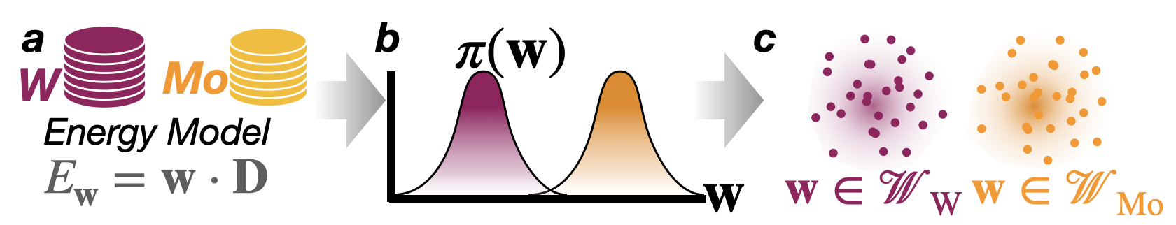
Figure 2: Producing ensemble of potential parameters for testing D-DOS in forward propagation. a) A linear MLIP (16) form is chosen to approximate ab initio databases, here of Mo and W. b) Misspecification-aware Bayesian regressionSwinburne and Perez (2025) returns a parameter posterior which is broad for simple MLIPs and diverse databases. c) The posterior is sampled to produce an ensemble of stable model parameters ${\mathbf{w}}\in\mathcal{W}_{\rm W}$ and ${\mathbf{w}}\in\mathcal{W}_{\rm Mo}$ used for testing.

VII.5 D-DOS score matching sampling campaign

As detailed in section VI, when using the harmonic isosurface function (30), our score matching sampling campaign reduces to sampling descriptor distributions on isosurfaces $\hat{\alpha}({\mathbf{X}})=\alpha$ defined by the Hessian $\bf H$ of some reference potential $E_{0}({\mathbf{X}})$. For momentum-dependent isosurface functions (32) we instead record samples from an ensemble of short NVE runs, which we explore in section VIII.2. We tested the harmonic isosurface function (30) using one Hessian ${\bf H}={\bf H}_{x}$ per phase for $x=\rm W,\,Mo,\ Fe$. Each Hessian was calculated using the appropriate lattice structure and the reference (loss minimizing) potential parameters ${\mathbf{w}}=\bar{{\mathbf{w}}}_{x}$ described in the previous section. With a given isosurface function $\hat{\alpha}({\mathbf{X}})$, we generated $\mathcal{O}(10^{3})$ independent samples on $\hat{\alpha}({\mathbf{X}})=\alpha$ for a range of $\alpha$ values at constant volume. It is simple to distribute sampling across multiple processors, as the harmonic isosurface samples are trivially independent (see appendix B). This enables a significant reduction in the wall-clock time for sampling over trajectory-based methods such as thermodynamic integration.
Our open-source implementationSwinburne and Marinica (2025) uses LAMMPSThompson et al. (2022) to evaluate SNAPThompson et al. (2015) descriptors; as a rough guide, with $N=\mathcal{O}(10^{2})$ atoms, the sampling campaign used to produce the results below required around $\mathcal{O}(10)$ seconds per $\alpha$ value on $\mathcal{O}(10^{2})$ CPU cores. A converged score model built from $\mathcal{O}(10)$ $\alpha$-values was thus achieved in under 5 minutes at each volume $V$ and Hessian choice ${\bf H}$. Algorithm 1 outlines the sampling campaign for each of the two isosurface functions we employ: $\hat{\alpha}({\mathbf{X}})$, equation (30), or $\hat{\alpha}({\mathbf{X}},{\bf P})$, equation (32). Use of momentum-dependent isosurfaces $\hat{\alpha}({\mathbf{X}},{\bf P})$ requires a single free energy estimate, which could be either from a separate D-DOS estimation or ‘traditional‘ sampling methods. In addition, to allowing for NVE sample decorrelation gives a factor 10 greater sampling effort, i.e. comparable with the effort for a single fixed model sampling. Computational demands quoted are when using $\hat{\alpha}({\mathbf{X}})$; future work will investigate schemes to further accelerate momentum-dependent $\hat{\alpha}({\mathbf{X}},{\bf P})$.

The final score model requires minimal storage, being only the $\mathcal{O}(100)$ scalars contained in the vector ${\bm{\Theta}}_{\alpha}$, equation (46), over a range of $\alpha$ values at constant $V$, ${\bf H}$. It is therefore possible to efficiently store many score models to investigate the influence of the reference model on free energy predictions. For example, section VIII.3 demonstrates how a D-DOS using ${\bf H}$ from $\bar{{\mathbf{w}}}_{\rm Mo}\in\mathcal{W}_{\rm Mo}$ can predict free energies from the W ensemble, ${\mathbf{w}}\in\mathcal{W}_{\rm W}$.

Table 1 provides a rough guide to the computational cost of existing methods, as reported in recent worksZhong et al. (2023); Menon et al. (2024); Castellano et al. (2024), alongside the D-DOS sampling scheme detailed above. As can be seen, D-DOS is at least an order of magnitude more efficient than TI and up to two orders of magnitude more efficient than AS, even before considering the massive reduction in wall-clock time due to parallelization. We again emphasize that in addition to the modest computational requirements of D-DOS, sampling is model-agnostic, only performed for a given choice of descriptor hyperparameters, system volume and function $\hat{\alpha}({\mathbf{X}})$ used for isosurface construction. Model agnosticism is the key innovation of the D-DOS approach, allowing rapid forward propagation for uncertainty quantification and, uniquely, back-propagation for inverse design goals. These unique abilities are demonstrated and tested in the next section.

Algorithm 1 Sampling for NVT estimator $\mathcal{F}_{{\mathbf{w}};{\bm{\Theta}}}(\beta)$

Crystal phase $p\in\mathcal{P}$, atom count $N$ and cell volume $V$

Reference potential $E_{0}({\mathbf{X}})$, typically $\bar{{\mathbf{w}}}^{\top}{\bm{\mathcal{D}}}$, $\bar{{\mathbf{w}}}\in\mathcal{W}$.

if $\hat{\alpha}=\hat{\alpha}({\mathbf{X}})$ then

  Calculate $\bf H$ of $E_{0}({\mathbf{X}})$ to give $\mathcal{F}_{0}(\beta)$ and thus $\mathcal{S}_{0}(\alpha)$

else $\hat{\alpha}=\hat{\alpha}({\mathbf{X}},{\bf P})$

  Calculate true $\mathcal{F}_{0}(\beta)$ and $\mathcal{U}_{0}(\beta)$ of $E_{0}({\mathbf{X}})$ to give $\mathcal{S}_{0}(\alpha)$

end if

Isosurface values $\alpha\in\mathcal{A}$ with $\alpha=\ln|\mathcal{U}_{0}(\beta)/{\rm U}_{0}|$

for  $\alpha\in\mathcal{A}$ do

  for $n\in N_{\rm samples}$, across parallel workers do

   if $\hat{\alpha}=\hat{\alpha}({\mathbf{X}})$ then

     Generate $\delta{\mathbf{X}}$ such that $\delta{{\mathbf{X}}}{\bf H}\delta{{\mathbf{X}}}$=$2N{\rm U}_{0}\exp(\alpha)$

     Record ${\bm{\mathcal{D}}}$

   else $\hat{\alpha}=\hat{\alpha}({\mathbf{X}},{\bf P})$

     Short NVE runs at $E={\rm U}_{0}\exp(\alpha)$

     Record ${\bm{\mathcal{D}}}\oplus K$

   end if

  end for

  Estimate ${\bm{\mu}}_{\alpha}$, ${\bm{\Sigma}}_{\alpha}$, solve (48) for vector ${\bm{\Theta}}_{\alpha}$

end for

Store ${\bm{\Theta}}=\{{\bm{\Theta}}_{\alpha}\}_{\alpha\in\mathcal{A}}$, NVT estimator $\mathcal{F}_{{\mathbf{w}};{\bm{\Theta}}}(\beta)$, $\forall{\mathbf{w}}\in\mathcal{W}$.

Method	$|\Delta\mathcal{F}|$	Steps	Steps/Worker	Agnostic
FEPFrenkel and Smit (1996) (II.2)	10	$\sim 10^{6}$	$\sim 10^{4}$	No
TIAthènes and Terrier (2017); Zhong et al. (2023) (II.1)	150	$\sim 10^{6}$	$\sim 10^{5}$	No
ASMenon et al. (2024) (II.3)	150	$\sim 10^{8}$	$\sim 10^{7}$	No
D-DOS	200	$\bf\sim 10^{5}$	$\bf\sim 10^{2}$	Yes

Table 1: Approximate comparison of computational cost for various methods to calculate solid-state vibrational free energies. $|\Delta\mathcal{F}|$: approximate maximum free energy difference that can be targeted at 1000 K in meV/atom, rising approximately proportionally with temperature. Steps: approximate number of force evaluations for 1-2 meV/atom convergence. Steps/Worker: approximate number of force evaluations per worker in a parallel sampling scheme, indicating the minimum wall-time. Agnostic: D-DOS sampling only needs to be conducted once for uniform approximation ability across broad range of potential parameters, while all other methods must be repeated, massively increasing the computational burden.

VIII Numerical experiments

In this section we detail numerical experiments, testing the D-DOS free energy estimates in forward and back-propagation. In forward propagation, our aim is to predict the free energy of all models ${\mathbf{w}}\in\mathcal{W}$ in a given ensemble, over a broad range of temperatures, from a single score matching campaign.

Accuracy in forward propagation, combined with robust misspecification-aware parameter uncertaintiesSwinburne and Perez (2025), clearly ensures accurate uncertainty quantification of free energies. A detailed investigation of D-DOS uncertainty quantification will be presented in a separate study, following recent work on static propertiesPerez et al. (2025). In back-propagation, we exploit access to parameter gradients of the free energy, equation (40), to fine-tune a given interatomic potential to match finite temperature properties. To our knowledge, this is the first demonstration of back-propagation being used to target phase boundaries in atomic simulation.

Section VIII.1 presents tests in forward propagation, predicting NVT free energies for bcc and A15 phases using a harmonic reference potential in $\hat{\alpha}({\mathbf{X}})$, equation (30). Section VIII.2 shows how predictions for the strongly anharmonic A15 phase can be systematically improved using the momentum-dependent isosurface function (32), invoking the curvature considerations raised in V.3. Section VIII.3 demonstrates the excellent alchemical transferability of the D-DOS approach, taking a D-DOS estimator using a harmonic reference for Mo to predict NVT free energies of models for W. Finally, sections VIII.4 and VIII.5 demonstrate how the D-DOS approach can be used in back-propagation for inverse design goals, starting from some reference potential $\bar{{\mathbf{w}}}$. Section VIII.4 adjusts the potential to match a given set of $\mathcal{F}(\beta)$ observations, regularizing against the original fit. Section VIII.5 extends this principle to minimize the $\alpha-\gamma$ free energy difference at a desired target temperature, targeting a phase boundary.

VIII.1 Prediction of NVT free energies

Our first results demonstrate the ability of our D-DOS sampling scheme to predict NVT free energies $\mathcal{F}_{\mathbf{w}}(\beta)$ for the bcc and A15 phases, using the ensemble of potentials ${\mathbf{w}}\in{\mathcal{W}}_{x}$, $x=\rm W,Mo$ described above and illustrated in Figure 3a).

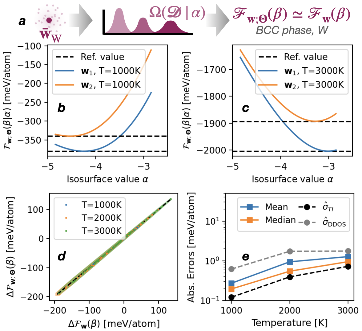
Figure 3: NVT free energy predictions in bcc phase of SNAP models ${\mathbf{w}}\in{\mathcal{W}}_{\rm W}$ from tungsten database. a) D-DOS sampling used $\hat{\alpha}({\bf X})$ function (30) using Hessian from $\bar{{\mathbf{w}}}_{\rm W}\in{\mathcal{W}}_{\rm W}$. b-c) Conditional free energy (36) $\mathcal{F}_{{\mathbf{w}};{\bm{\Theta}}}(\beta|\alpha)$ with $\alpha$ at T=1000 K (left) and T=3000 K (right). Horizontal dashed lines give reference values from thermodynamic integration. d) Parity plot for three temperatures. Note the large (300 meV) spread of values at high temperatures. Shaded areas are convex hull around D-DOS predictions with errors, i.e. $\mathcal{F}_{{\mathbf{w}};{\bm{\Theta}}}(\beta|\alpha)\pm\hat{\sigma}_{\rm DDOS}$. e) Mean and median absolute errors, showing sub meV/atom accuracy, along with estimations from thermodynamic integration ($\sigma_{\rm TI}$) and D-DOS ($\hat{\sigma}_{\rm DDOS}$).

Figure 3 shows D-DOS predictions for bcc phases against the corresponding thermodynamic integration (TI) calculations. The D-DOS was estimated by score matching on isosurfaces $\hat{\alpha}({\mathbf{X}})=\alpha$, equation (30), using a single Hessian matrix ${\bf H}$ from the same ensemble. Panels b) and c) display how $\mathcal{F}_{{\mathbf{w}};{\bm{\Theta}}}(\beta|\alpha)$ depends on $\alpha$ for two different potentials ${\mathbf{w}}_{1},{\mathbf{w}}_{2}\in\mathcal{W}_{\rm W}$. The minimization procedure can be efficiently achieved, with the full free energy estimation procedure requiring around 10-100 microseconds of CPU effort depending on the complexity of the score model employed; in the current implementation, the effort scales approximately linearly with the number of feature functions $F$. Panels d) and e) show the excellent approximation ability of the D-DOS estimator despite the high degree of diversity across the ensemble. Importantly, the predicted D-DOS errors are excellent estimates of the actual errors. In 3d) we subtract the free energy of the harmonic system used to build $\hat{\alpha}({\mathbf{X}})$, thus displaying the explicit (NVT) anharmonicity captured by the D-DOS estimator, with typical absolute values of 150 meV/atom at 3000K, with ensemble variations of around 300 meV/atom. The mean absolute errors of 1 meV/atom, or 1/40 kcal/mol, even at these elevated temperatures, represent a key numerical result of this paper, showing that the presented model-agnostic approach is both more efficient and directly comparable to existing state-of-the-art sampling approaches.

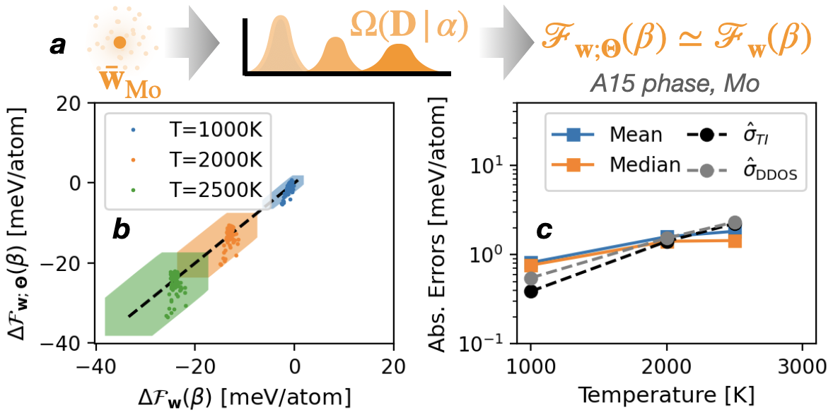
Figure 4: NVT free energy predictions in A15 phase of SNAP models from molybdenum database. a) D-DOS sampling employed $\hat{\alpha}({\bf X})$, equation (30), built with $\bar{{\mathbf{w}}}_{\rm Mo}$. The testing potential ensemble ${\mathbf{w}}\in{\mathcal{W}}_{\rm Mo}$ was less diverse to ensure stability of TI calculations. b) Parity plot at three temperatures. c) Mean and median absolute errors over $\mathcal{W}_{\rm Mo}$.

Figure 4 shows D-DOS predictions for the NVT free energy of the metastable A15 phases for parameters from the Mo ensemble, ${\mathbf{w}}\in{\mathcal{W}}_{\rm Mo}$. The metastability of the A15 phase significantly reduces the diversity of potentials whose free energy can stably be estimated via TI. Similarly, the estimated errors in the final values from TI are correspondingly larger. For D-DOS, however, there are no stability issues- we only require the potential $\bar{{\mathbf{w}}}\in{\mathcal{W}}_{\rm Mo}$ used to build the isosurface has a Hessian with no negative eigenvalues. This opens many perspectives for sampling of unstable phases, as we discuss in IX. As can be seen in figure 5 the D-DOS estimates retain mean average errors of less than 2meV/atom at 2500 K, and, crucially, the propagated error estimates envelope the true errors. At higher temperatures, we see that the ensemble average sampling errors from D-DOS and TI are almost identical.

VIII.2 Influence of the isosurface function

While the ensemble used for A15 predictions of Mo, figure 4, gave good predictions of NVT free energies using a harmonic reference potential in the isosurface function $\hat{\alpha}({\mathbf{X}})$, the performance for W was poorer, reaching 8.5 meV/atom at 2500 K as shown in figure 5d-e). Importantly, D-DOS error estimates are similarly large, meaning our estimator is correctly indicating the isosurface function is poorly chosen in this case.

As discussed in V.3, application of Laplace’s method requires minimizing an estimate $\mathcal{F}_{{\mathbf{w}};{\bm{\Theta}}}(\beta|\alpha)$ with respect to $\alpha$, equation (50), which will be more robust to noise if the $\alpha$-curvature $\partial_{\alpha}^{2}\mathcal{F}(\beta|\alpha)$ is higher. We thus expect isosurface functions which give a higher curvature in $\mathcal{F}_{{\mathbf{w}};{\bm{\Theta}}}(\beta|\alpha)$ will have lower predicted and observed errors. In figure 5b) we show $\mathcal{F}(\beta|\alpha)$ for a given potential ${\mathbf{w}}_{1}\in\mathcal{W}_{\rm W}$ using $\hat{\alpha}({\mathbf{X}})$, which employs a harmonic potential as defined in (30), and the momentum-dependent isosurface $\hat{\alpha}({\mathbf{X}},{\bf P})$, which uses a general interatomic potential as defined in (32). As can be seen in 5b) for ${\mathbf{w}}={\mathbf{w}}_{1}$ and in 5c) across the whole ensemble, the momentum-dependent isosurface gives significantly higher curvature with $\alpha$. Using $\hat{\alpha}({\mathbf{X}},{\bf P})$ for sampling then gives significantly lower predicted and observed errors, remaining within the 1-2 meV/atom limit (1.5 meV/atom at 2500 K) required for phase stability.

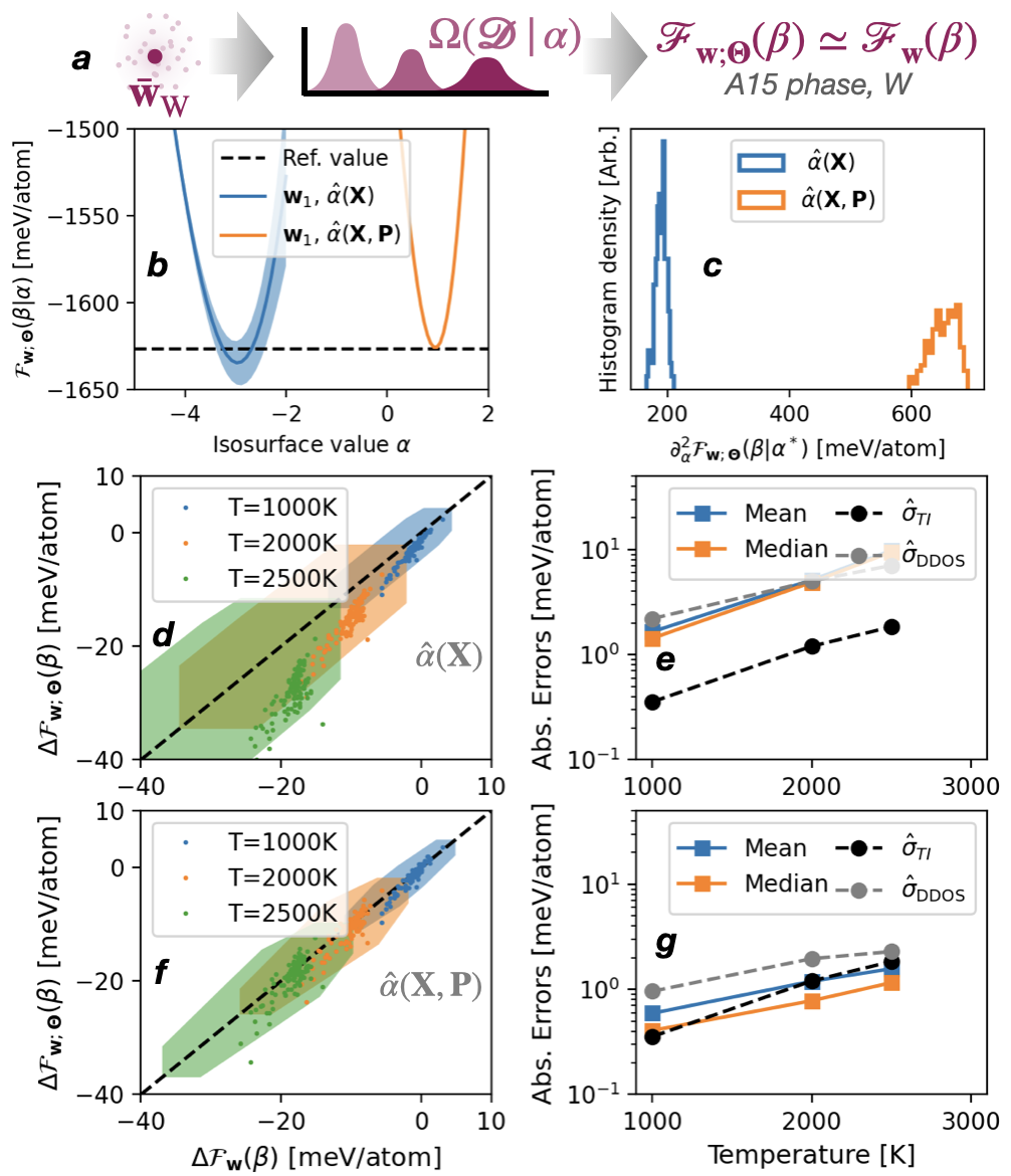
Figure 5: Influence of isosurface function in NVT free energy predictions of SNAP models for W in the A15 phase, a strongly anharmonic structure which was only stable in a tightly clustered set of ensemble members ${\mathbf{w}}\in\mathcal{W}$. a) D-DOS sampling employed $\hat{\alpha}({\mathbf{X}})$ and $\hat{\alpha}({\mathbf{X}},{\bf P})$ with ${\mathbf{w}}=\bar{{\mathbf{w}}}_{\rm W}$ (see IV.3). b) Conditional free energy (36) at T=2500 K, with propagated errors, for a representative potential ${\mathbf{w}}_{1}\in\mathcal{W}_{\rm W}$, using $\hat{\alpha}({\mathbf{X}})$ or $\hat{\alpha}({\mathbf{X}},{\bf P})$. c) $\hat{\alpha}({\mathbf{X}},{\bf P})$ gives a conditional free energy with a higher curvature, leading to increased accuracy with Laplace’s method (see V.3) and lower propagated errors from the score matching model. d-e) Free energy prediction with $\hat{\alpha}({\mathbf{X}})$ gives large predicted and observed errors, reaching 8.5 meV/atom at 2500 K, consistent with a) and the low curvature of $\mathcal{F}(\beta|\alpha)$. f-g) Use of $\hat{\alpha}({\mathbf{X}},{\bf P})$ brings back the low predicted and observed errors required for phase prediction, within the target range of 1-2 meV/atom (1.5 meV/atom at 2500 K).

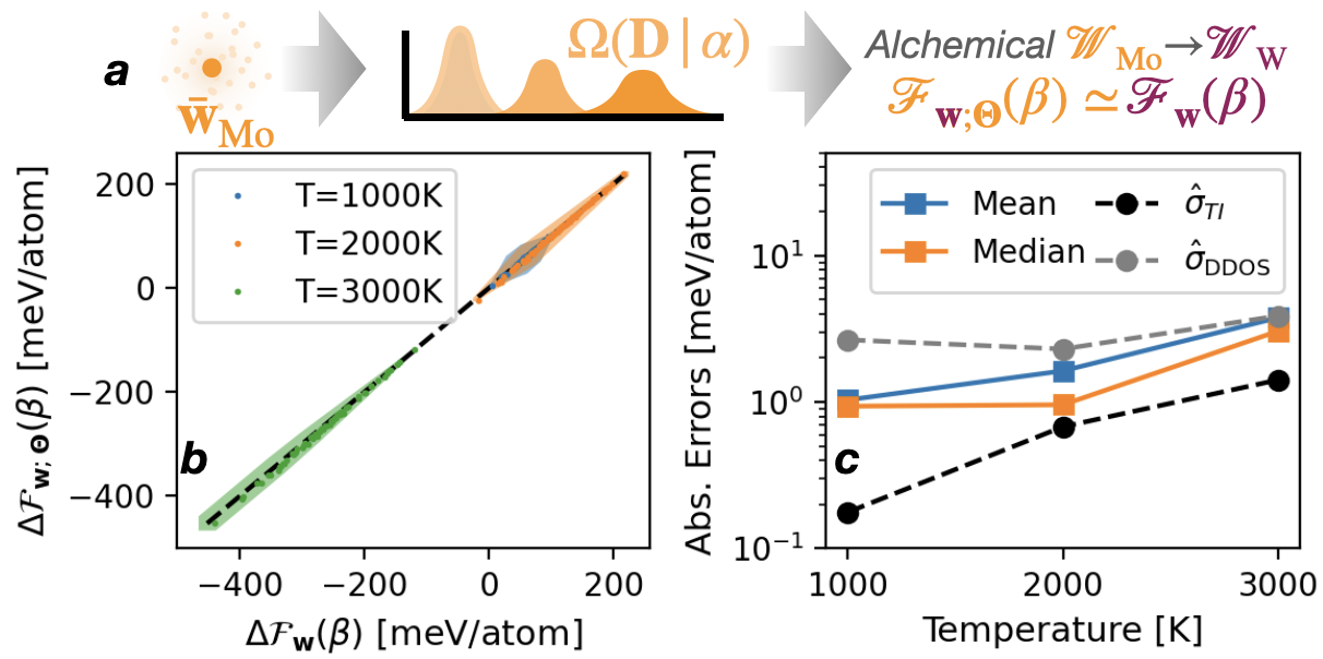
Figure 6: Alchemical transferability. a) D-DOS sampling with $\hat{\alpha}({\bf X})$, equation (30), built with reference Mo potential $\bar{{\mathbf{w}}}_{\rm Mo}$. However, the testing ensemble is for W, ${\mathbf{w}}\in\mathcal{W}_{\rm W}$, as shown in figure 3. b) Parity plot at three temperatures with propagated errors as in other ., with median accuracy of 2 meV/atom over a 600 meV/atom range. c) Mean and median absolute errors over $\mathcal{W}_{\rm W}$. Predicted D-DOS errors propagated from score matching (VI.2) tightly bound true errors.

VIII.3 Alchemical transferability

As a final stringent test of D-DOS sampling in forward propagation, figure 6 shows predictions of the same bcc NVT free energies for the W ensemble $\mathcal{W}_{\rm W}$ presented in figure 3, but now using a D-DOS estimator with $\hat{\alpha}({\mathbf{X}})$ built using the Hessian from a representative potential $\bar{{\mathbf{w}}}_{\rm Mo}$ from the Mo ensemble $\mathcal{W}_{\rm Mo}$. Despite the significant increase in explicit anharmonicity due to the change of reference system (6b), we see that performance is only slightly reduced, with errors remaining at 1-2 meV/atom (6c), within the target range of our state-of-the-art thermodynamic calculations. These results provide compelling evidence that the approach outlined here opens many perspectives for ‘universal’ or alchemical sampling, which we discuss further in IX.

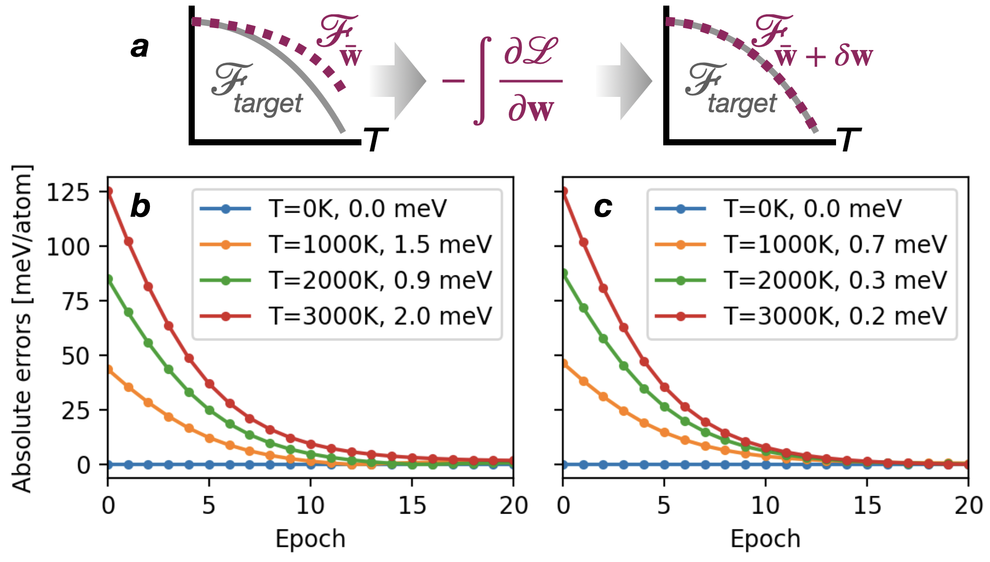
Figure 7: Fine-tuning potentials to match target W bcc NVT free energy values. a) Access to parameter gradient of free energy allows for inclusion of finite temperature properties in potential training. b-c) Error against four target free energy values of single $\bar{{\mathbf{w}}}+\delta{\mathbf{w}}$ trajectory under gradient descent. b) Target set to the 15th percentile in free energy over $\mathcal{W}_{\rm W}$ at each temperature. c) Target values calculated with a single model from $\mathcal{W}_{\rm W}$, a specified problem with lower errors.

VIII.4 Targeting of NVT free energies

In the next two subsections, we turn to back-propagation of parameter variations, a long-standing goal of atomic simulations which, to the best of our knowledge, has never been achieved for complex thermodynamic quantities such as the free energy, which cannot be expressed as a simple expectation.

We first consider the ‘fine-tuning’ of an initial interatomic potential parameter $\bar{{\mathbf{w}}}$, targeting some reference NVT free energies. While we consider arbitrary targets, in applications one would target ab initio values obtained from a multi-stage stratified sampling schemeCastellano et al. (2024), to enforce consistency during the training of a general purpose MLIP.

In our inverse design procedure, we start with some regularization term $\mathcal{L}_{0}({\mathbf{w}})$, i.e. the training loss or the negative log likelihood from Bayesian inferenceSwinburne and Perez (2025). Our primary target is a set of NVT free energies $\{\mathcal{F}(\beta_{t})\}$ at a range of inverse temperatures $\{\beta_{t}\}$, giving an objective function

$$\mathcal{L}({\mathbf{w}})=\sum_{t}\|\mathcal{F}_{{\mathbf{w}};{\bm{\Theta}}}(\beta_{t})-\mathcal{F}(\beta_{t})\|^{2}+r\mathcal{L}_{0}({\mathbf{w}}),$$ (51)

where $r$ controls the regularization strength. Access to the parameter gradient (40) allows minimization through simple application of gradient descent, updating parameters through ${\mathbf{w}}_{n+1}={\mathbf{w}}_{n}-\delta\nabla_{\mathbf{w}}\mathcal{L}({\mathbf{w}}_{n})$.

Figure 7 shows the result of this process for two different target free energies; in figure 7b), the target is simply the 15th percentile value at each temperature across the W ensemble $\mathcal{W}_{\rm W}$, showing maximum error of 2 meV/atom at 3000 K. In this case, the target is misspecified, i.e. it is not clear that a single choice of MLIP parameters is able to match the target value, mimicking the realistic design case where $\{\mathcal{F}(\beta_{t})\}$ is obtained from ab initio data. Nevertheless, our minimization approach smoothly converges to within 2 meV/atom at high temperature. Figure 7c) shows a specified target, using the free energies of a single model calculated through thermodynamic integration, which has similar deviation from the free energies of $\bar{{\mathbf{w}}}$ as the first target. In this case, we obtain essentially perfect agreement (within the sampling uncertainty) of less than 1 meV/atom at all temperatures. These results represent a second key result of this paper, a demonstration that finite temperature material properties can be included in the objective functions for negligible additional cost; as mentioned above, evaluation of the free energy and its gradient requires only microseconds of CPU effort, with no additional atomistic sampling.

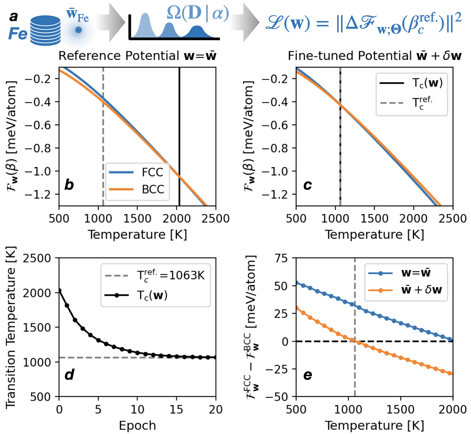
Figure 8: Inverse fine-tuning to target the $\alpha\to\gamma$ transition in Fe. a) From multiphase training data in Fe, we perform D-DOS sampling with $\hat{\alpha}({\bf X})$, using $\bf H$ from the reference Fe potential $\bar{{\mathbf{w}}}_{\rm Fe}$. b) NVT free energies in fcc and bcc phases of $\bar{{\mathbf{w}}}_{\rm Fe}$, using equilibrium volume at $T^{\rm ref}_{c}=1063$ K. The observed transition occurs at $T_{c}(\bar{{\mathbf{w}}})=2030$ K. c) The fine-tuned potential $\bar{{\mathbf{w}}}+\delta{\mathbf{w}}$ has the correct transition temperature. d) The transition temperature smoothly decays during fine-tuning. e) Free energy difference between fcc and bcc phases with temperature for ${\mathbf{w}}=\bar{{\mathbf{w}}}$ (blue) and ${\mathbf{w}}=\bar{{\mathbf{w}}}+\delta{\mathbf{w}}$ (orange). Despite the small (40 meV/atom) change in free energy, the transition temperature is reduced by nearly 1000 K, demonstrating the sensitivity of phase stability to small changes in interatomic potential parameters.

VIII.5 Targeting $\alpha\to\gamma$ transition temperature in Fe

As a final example, we demonstrate how back-propagation allows for the targeting of phase transition temperatures, to our knowledge, a unique ability of the D-DOS procedure. As above, targets could be calculations from established schemesCastellano et al. (2024) to enforce consistency during general purpose potential training, prescribed from higher level simulations to enforce consistency within multi-scale modelsChen and Zhao (2022) or to experimental data, in top-down training schemesThaler et al. (2022).

Our demonstration targets the bcc-fcc, or $\alpha\to\gamma$, transition in Fe. While known to be due to the loss of ferromagnetic orderingMa et al. (2017), in this example of back-propagation we employ non-magnetic SNAP models of Fe. Our starting point is a previously published set of SNAP parameters $\bar{{\mathbf{w}}}_{\rm Fe}$Goryaeva et al. (2021b) which was designed primarily for the simulation of point and extended defects in the bcc phase. While the model supports a stable fcc phase, the initial $\alpha\to\gamma$ transition temperature is over 2000 K, significantly above the target value of 1063 K.

Using $\bar{{\mathbf{w}}}_{\rm Fe}$ to generate harmonic isosurface functions $\hat{\alpha}({\mathbf{X}})$, equation (30), for fcc and bcc phases, a D-DOS score matching campaign produced estimators for both phases over a small range of atomic volumes, allowing calculation of NPT free energies $\mathcal{G}_{{\mathbf{w}};{\bm{\Theta}}}(\beta)$, as detailed in section II.1, equation (8). With estimators for both the fcc and bcc free energies at the desired critical temperature ${\rm T}_{c}=1063$K, the objective function reads

$$\mathcal{L}({\mathbf{w}})=\|\mathcal{G}_{{\mathbf{w}};{\bm{\Theta}}}(\beta_{c},{\rm bcc})-\mathcal{G}_{{\mathbf{w}};{\bm{\Theta}}}(\beta_{c},{\rm fcc})\|^{2}+r\mathcal{L}_{0}({\mathbf{w}}),$$ (52)

where $\beta_{c}=1/({\rm k_{B}T}_{c})$ and as in (51) $\mathcal{L}_{0}({\mathbf{w}})$ is the training loss function with a regularization parameter $r\geq 0$ and $\beta_{c}=1/{\rm k_{B}T}_{c}$. Clearly, minimization of the first term will ensure a predicted phase transition at $\rm T_{c}$ as the Gibbs free energies are equal. As in the previous section, parameters are updated by gradient descent, using (40) to evaluate $\nabla_{\mathbf{w}}\mathcal{L}({\mathbf{w}})$ by the chain rule.

As shown in figure 8, this inverse fine-tuning procedure enables finding the subtle changes in potential parameters required to reproduce the desired phase boundary, reducing the $\alpha\to\gamma$ transition temperature from 2030 K to 1063 K, with the gradient descent smoothly converging, figure 8d). While the total free energy changes were relatively small, on the order of 30 meV/atom, figure 8e) demonstrates the consequence on the phase boundary: as the free energy gradient with temperature is only around 0.03 meV/atom/K, a change of 30 meV/atom results in a 1000 K change in phase transition temperature.

IX Discussion

We end this paper with a brief outline of the many perspectives for model agnostic sampling with D-DOS approach, within condensed matter physics and materials science and also more widely, many of which will be investigated in future work.

IX.1 Liquid and dynamically unstable phases

The momentum-dependent isosurface function (32) only requires the ability to perform NVE dynamics with the reference potential $E_{0}({\mathbf{X}})$ and can thus be applied to evaluate free energies of liquids or dynamically unstable solidsPark et al. (2024). Section VIII.2 demonstrated that use of (32) significantly improved prediction accuracy when applied to the strongly anharmonic A15 phase in W. Of equal importance, the predicted error bounds also significantly reduced. A full study of liquid free energies and thus melting transitions within the D-DOS approach will be the subject of a forthcoming study. For dynamically unstable (entropically stabilized) systems the conditional descriptor entropies may be multi-modal, potentially requiring more advanced score models employing e.g. low-rank tensor approximationsCui et al. (2023); Darby et al. (2023); Sherman and Kolda (2020) or neural-networksSong et al. (2020), beyond the simple low-rank score model employed here. We anticipate that integrating these more flexible density estimation models will open many perspectives for sampling complex material systems.

IX.2 Fine-tuning of foundational MLIPs

Section III.1 discussed the applicability of D-DOS beyond the linear MLIPs employed in our numerical experiments (section VII.1). In particular, the D-DOS scheme is well-suited to the fine-tuning of message passing neural network (MPNN) interatomic potentialsMusaelian et al. (2023); Batzner et al. (2022); Batatia et al. (2022); Cheng (2024), which have gained prominence due to their ‘foundational’ ability to approximate broad regions of the periodic tableBatatia et al. (2023); Bochkarev et al. (2024). While MPNN training is a deep learning procedure involving millions of model weights, fine-tuning schemes typically only target a small number of parameters in the MPNN readout layer, which can be expressed in the general linear form (16). For example, uncertainty quantification schemes designed for linear models have recently been applied to e.g. the MACE-MPA-0 foundation modelPerez et al. (2025). The ability to fine-tune foundation models on available phase diagram data, either from experiment or from reference calculations, is actively sought in atomic modelling and will be investigated in the near future. In particular, the light computational demand and storage requirements of D-DOS mean production of a ‘foundational’ D-DOS sampling library for foundational MPNNs is feasible and indeed desirable, allowing practitioners to rapidly assess how e.g. fine-tuning on additional training data improves free energy predictions.

Beyond physics models, a broad range of computational tasks reduce to evaluating high-dimensional integrals. We here highlight two well known examples which can be cast to the generalized linear form (16) amenable to D-DOS estimation.

IX.3 Generalized Ising Models

Generalized Ising models are widely used in condensed matter physics and materials science. For example, the popular cluster expansionEkborg-Tanner et al. (2024) model is used to approximate the configurational entropy of multi-component lattice systems. Cluster expansion models have energies of the form (16), where descriptor features ${\bm{\mathcal{D}}}$ (typically denoted as $\bm{\Gamma}$ in the cluster expansion literature) are correlation functions of some multi-component lattice and ${\mathbf{w}}$ (typically denoted as $\bf J$) is fit to ab initio data. The central difference is that the configuration space is no longer a vector ${\mathbf{X}}\in\mathbb{R}^{3N}$ but $\bm{\sigma}\in[1,S]^{N}$, the discrete set of all $S$-component configurations across $N$ lattice sites. Generalized Ising models have a rich phenomenology, in particular second order phase transitions, and the development of efficient sampling methods is an active area of researchZhang et al. (2020); Marchand et al. (2023). However, we anticipate that the D-DOS approach could be applied in some settings, e.g. for model-agnostic sampling of equilibrium averages central to the cluster expansion modelsEkborg-Tanner et al. (2024), with the same advantages for uncertainty quantification and inverse design as shown for atomistic systems.

IX.4 Probabilistic learning and Bayesian inference

Probabilistic machine learning and Bayesian inference both require fast evaluation of high dimensional integralVon Toussaint (2011); Bhat and Kumar (2010); Lotfi et al. (2022). A quite direct analogy with D-DOS can be found if we equate ${\mathbf{X}}$ with model parameters, ${\mathbf{w}}$ with hyperparameters and the free energy with e.g. the log evidence per parameter or the log of the posterior predictive distribution, in the limit of a very large number of model parametersDuffield et al. (2024). In this setting the common Laplace approximation used to evaluate integrals in Bayesian inference exactly corresponds here to the harmonic approximation used for the construction of $\hat{\alpha}({\mathbf{X}})$, equation (30). We can thus apply the D-DOS approach if we can write the log likelihood as the sum of the harmonic expansion used in the Laplace approximation and a generalized linear feature model ${\mathbf{w}}\cdot{\bm{\mathcal{D}}}$. In this setting the model-agnostic estimation of D-DOS would allow rapid, differentiable exploration of the hyperparameter dependence on model predictions actively sought in Bayesian machine learningBlondel et al. (2022).

X Conclusions

In this study, we have revised traditional methods to estimate the vibrational free energy of atomic systems by proposing a novel approach that leverages descriptors, high-dimensional feature vectors of atomic configurations. We introduced the foundations for estimating key quantities of interest in this high-dimensional descriptor space, such as the descriptor density of states and corresponding entropy. The present reformulations introduce a model-agnostic sampling scheme for atomic simulation.

Rather than existing methods which return free energy estimates for a specific value of interatomic potential parameters, we instead return an estimator that can predict free energies over a broad range of model parameters. This is a significant change in approach that not only allows for rapid forward propagation of parameter uncertainties to finite temperature properties, but also uniquely allows for inverse fine-tuning of e.g. phase boundaries through back-propagation, both long-desired capabilities in computational materials science.

Central to our scheme is the descriptor density of states (D-DOS), a multidimensional generalization of the energy density of states. We showed how score matching the descriptor entropy (log D-DOS) enables free energy estimation without numerical integration for the wide class of interatomic potentials that can be expressed as a linear model of descriptor features. A large range of tasks in computational science reduce to evaluating high-dimensional integrals, and thus many can be cast in a form directly analogous to the free energy estimation problem D-DOS solves, some of which we outlined above. We fully anticipate that more examples can be found which would allow the application of the D-DOS approach to a wide range of computational tasks.

XI Acknowledgments

We gratefully acknowledge the hospitality of the Institute for Pure and Applied Mathematics at University of California, Los Angeles, the Institute for Mathematical and Statistical Innovation at the University of Chicago and the Institut Pascal at Université Paris-Saclay, which is supported by ANR-11-IDEX-0003-01. TDS gratefully acknowledges support from ANR grants ANR-19-CE46-0006-1, ANR-23-CE46-0006-1, IDRIS allocation A0120913455 and an Emergence@INP grant from the CNRS. All authors acknowledge the support from GENCI - (CINES/CCRT) computer centre under Grant No. A0170906973.

XII Data Availability

After peer review, an open source code repository of our score matching scheme, enabling D-DOS estimation for any descriptor implemented in the LAMMPSThompson et al. (2022) molecular dynamics code, will be available at www.github.com/tomswinburne/DescriptorDOS.git.

Appendix A Summary of Laplace’s method

Laplace’s method, also known as the steepest descents method, is a well-known identity allowing the evaluation of an integral of an exponentiated function multiplied by a large number. We provide a brief summary of the method here, and we refer the reader to e.g. (Wong, 2001) for further information. The method applies to a function $f({\bf x})$, ${\bf x}\in\mathbb{R}^{n}$ which is twice differentiable. We partition the domain $\mathbb{R}^{n}=\cup_{l=1}^{L}\mathcal{R}_{l}$ into regions $\mathcal{R}_{l}$ each with a single maximum ${\bf x}^{*}_{l}$, where the negative Hessian matrix ${\bf H}_{l}=-\nabla_{\bf x}\nabla^{\top}_{\bf x}f_{|\mathcal{R}_{l}}\in\mathbb{R}^{n\times n}$ of $Nf({\bf x})$ has $\mathcal{O}(n)$ positive eigenvalues $\lambda_{p}\geq 0$, no negative eigenvalues, and all entries of ${\bf H}_{l}$ (and thus all $\lambda_{p}$) are independent of $N$. In the limit $N\to\infty$ the integral in $\mathcal{R}_{l}$ is dominated by the maximum ${\bf x}^{*}_{l}$. Proof of Laplace’s method uses Taylor expansions of $f({\bf x})$ around ${\bf x}^{*}_{l}$ to provide upper and lower bounds, which in the limit $N\to\infty$ both converge to the same Gaussian integral, giving

$$\lim_{N\to\infty}\int_{\mathbb{R}^{n}}\exp[Nf({\bf x})]{\rm d}{\bf x}=\sum_{l=1}^{L}\frac{\exp[Nf({\bf x}^{*}_{l})]}{\sqrt{(2\pi N)^{n}|{\bf H}_{l}|}}.$$ (53)

In the case of constant $n$ as $N\to\infty$ it is simple to show that the limiting form of the log integral is

$$\lim_{N\to\infty}\frac{1}{N}\ln\int_{\mathbb{R}^{n}}\exp[Nf({\bf x})]{\rm d}{\bf x}=\max_{l}f({\bf x}^{*}_{l}).$$ (54)

where we use the fact that

$$\lim_{N\to\infty}\frac{1}{N}\ln\sqrt{(2\pi N)^{n}|{\bf H}_{l}|}=\lim_{N\to\infty}\frac{1}{2N}\left(n\ln|2\pi N|+\sum_{p=1}^{n}\ln\lambda_{p}\right)=0.$$ (55)

as $\lim_{N\to\infty}n/N=0$ and $\lim_{N\to\infty}(1/N)\ln|N|=0$. When the argument of the function has dimension which scales with $N$, i.e. $n=rN$, $r>0$, ($r=3$ for Hessians), the above simplification does not hold. In general, the integral will depend on higher order gradients to correctly take the limit. Note that the above is distinct from the common use of Laplace’s method to approximate the partition function integral $\int_{\mathbb{R}^{3N}}\exp[-\beta E({\bf X})]{\rm d}{\bf X}$; although the dimension of $\bf X$ is extensive, in this case Laplace’s method is used in the low temperature limit $\beta\to\infty$, rather than $N\to\infty$.

Appendix B Isosurface for a harmonic solid

B.1 Sampling

For solid systems we use a harmonic reference potential energy $E_{0}({\mathbf{X}})$ and isosurface function $\hat{\alpha}({\bf X})$

$$E_{0}({\mathbf{X}})\equiv\frac{[{\mathbf{X}}-{\mathbf{X}}_{0}]^{\top}{\bf H}[{\mathbf{X}}-{\mathbf{X}}_{0}]}{2N},\quad\hat{\alpha}({\mathbf{X}})\equiv\ln\left|\frac{\hat{E}_{0}({\bf X})}{{\rm U}_{0}}\right|.$$ (56)

We assume that ${\bf H}$ has $3N^{\prime}=3N-3$ positive eigenvalues $\nu_{l}>0$, $l>3$ with normalized eigenvectors ${\bf v}_{l}$. We can thus define normal mode coordinates $\tilde{\rm X}_{l}\equiv{\bf v}_{l}\cdot{\mathbf{X}}/\sqrt{\nu_{l}}$, $l>3$. In addition, we have $3$ zero modes $\nu_{l}=0$, $l=1,2,3$ with eigenvectors selecting the center of mass $\bar{\bf x}$ multiplied by $\sqrt{N}$, i.e. $\tilde{\rm X}_{l}\equiv\sqrt{N}\bar{\rm x}_{l}$, $l=1,2,3$, which meaning we can always ensure normal modes have zero net displacement, i.e. enforce ${\bf v}_{l}\cdot{\bf 1}=0$, $l>3$.

In normal mode coordinates, the energy writes

$$E_{0}({\mathbf{X}})=\frac{1}{2N}\sum_{l=4}^{l=3N}{\nu_{l}}\|{\bf v}_{l}\cdot{\mathbf{X}}\|^{2}=\frac{1}{2N}\sum_{l=4}^{l=3N}\tilde{\rm X}^{2}_{l}=\frac{\tilde{\rm R}^{2}}{2N}.$$ (57)

Sampling the isosurface $\hat{\alpha}({\mathbf{X}})=\alpha$ is clearly equivalent to sampling $E_{0}({\mathbf{X}})={\rm U}_{0}\exp(\alpha)$, which in normal mode coordinates amounts to sampling the surface of a hypersphere with radius $\tilde{\rm R}=\sqrt{2N{\rm U}_{0}}\exp(\alpha/2)$.

With a unit vector ${\bf u}=[{\rm u}_{1},\dots,{\rm u}_{3N^{\prime}}]\in\mathbb{R}^{3N^{\prime}}$ on the $3N^{\prime}$ dimensional hypersphere, isosurface samples can then be produced through

$${\mathbf{X}}_{\alpha}[{\bf u}]\equiv{\mathbf{X}}_{0}+\sum_{l=1}^{3N^{\prime}}\sqrt{\frac{2N{\rm U}_{0}\exp(\alpha)}{\nu_{l}}}{\rm u}_{l}{\bf v}_{l},\quad\Rightarrow\quad E_{0}\left({\mathbf{X}}_{\alpha}[{\bf u}]\right)={\rm U}_{0}\exp(\alpha)\sum_{l=1}^{3N^{\prime}}{\rm u}^{2}_{l}={\rm U}_{0}\exp(\alpha).$$ (58)

Importantly, the sampling procedure can be trivially parallelized as we can generate independent samples $\{{\bf u}\}$ on each parallel worker, providing each worker with a unique seed for pseudo-random number generation.

B.2 Isosurface volume and isosurface entropy

For harmonic isosurface functions $\hat{\alpha}({\mathbf{X}})$, we can express the isosurface volume (24) in normal mode coordinates using standard expressions for change of variables:

$$\Omega(\alpha) =\int_{\mathbb{R}^{3N}}\delta(\hat{\alpha}({\mathbf{X}})-\alpha){\rm d}{{\mathbf{X}}}$$ (59)

$$=\frac{V}{\prod_{l=4}^{3N}\sqrt{\nu_{l}}}\int_{\mathbb{R}^{3N^{\prime}}}\delta\left(\ln\left|\sum_{l=4}^{3N}\tilde{\rm X}_{l}^{2}/(2N)\right|-\alpha\right)\prod_{l=4}^{3N}{\rm d}\tilde{\rm X}_{l}.$$ (60)

Converting to spherical coordinates we find, using the expression for the surface area of a unit sphere in $3N^{\prime}$ dimensions as $S_{3N^{\prime}}=2{\pi}^{3N^{\prime}/2}/\Gamma(3N^{\prime}/2)$, then again changing variables with ${\rm d}\tilde{\rm R}=\sqrt{N{\rm U}_{0}/2}\exp(\alpha/2){\rm d}\alpha$, we find that

$$\Omega(\alpha) =\frac{2V{\pi}^{3N^{\prime}/2}}{\Gamma(3N^{\prime}/2)}\int_{\mathbb{R}_{+}}\delta\left(\ln\left|\tilde{\rm R}^{2}/(2N)\right|-\alpha\right)\tilde{\rm R}^{3N^{\prime}-1}{\rm d}\tilde{\rm R}$$ (61)

$$=\frac{V\sqrt{\rm U}^{3N^{\prime}}_{0}}{\prod_{l=4}^{3N}\sqrt{\nu_{l}}}\frac{\sqrt{2\pi N}^{3N^{\prime}}}{\Gamma(3N^{\prime}/2)}\exp(3N\alpha/2).$$ (62)

We thus see that the isosurface volume for harmonic solids has the general form

$$\Omega(\alpha)=\Omega_{0}\exp(3N\alpha/2),\quad\Omega_{0}=\frac{V\sqrt{\rm U}^{3N^{\prime}}_{0}}{\prod_{l=4}^{3N}\sqrt{\nu_{l}}}\frac{\sqrt{2\pi N}^{3N^{\prime}}}{\Gamma(3N^{\prime}/2)},$$ (63)

giving an isosurface entropy

$$\mathcal{S}_{0}(\alpha)\equiv\lim_{N\to\infty}\frac{1}{N}\ln|\Omega(\alpha)/\lambda^{3N}_{0}(\beta)|=S_{0}+3\alpha/2,\quad S_{0}=\ln|\lambda^{3}_{0}(\beta)|+(1/N)\ln|\Omega_{0}|.$$ (64)

While we can simplify the expression for the $\ln\Omega_{0}$ using Stirling’s approximation we shall see this is not required.

B.3 Isosurface entropy and connection to harmonic free energy

Using standard Gaussian integrals, the partition function of a harmonic system reads, with $\lambda_{0}(\beta)=h\sqrt{\beta/(2\pi m)}$,

$$Z_{0}(\beta)=\frac{1}{\lambda^{3N}_{0}(\beta)}\int_{\mathbb{R}^{3N}}\exp[-N\beta E_{0}({\mathbf{X}})]{\rm d}{\mathbf{X}}=\frac{V}{\lambda^{3N}_{0}(\beta)}\prod_{l=4}^{3N}\frac{1}{\sqrt{2\pi\beta\nu_{l}}},$$ (65)

giving a free energy in the limit $N\to\infty$

$$\mathcal{F}_{0}(\beta)\equiv\lim_{N\to\infty}\frac{-1}{N\beta}\ln|Z_{0}(\beta)|=\frac{1}{N\beta}\sum_{l=4}^{3N}\ln\left|\beta\hbar\sqrt{\nu_{l}/m}\right|.$$ (66)

We can also write $\mathcal{F}_{0}(\beta)$ using the isosurface entropy defined in equation (64) and applying Laplace’s method, i.e.

$$\beta\mathcal{F}_{0}(\beta) =\lim_{N\to\infty}\frac{-1}{N}\ln\left|\frac{1}{\lambda^{3N}_{0}(\beta)}\int_{\mathbb{R}}\Omega(\alpha)\exp(-N\beta{\rm U}_{0}e^{\alpha}){\rm d}\alpha\right|$$ (67)

$$=\lim_{N\to\infty}\frac{-1}{N}\ln\left|e^{NS_{0}}\int_{\mathbb{R}}\exp(3N\alpha/2-N\beta{\rm U}_{0}e^{\alpha}){\rm d}\alpha\right|,$$ (68)

$$=\min_{\alpha}{\rm U}_{0}e^{\alpha}-3\alpha/2-S_{0},$$ (69)

$$={\rm U}_{0}e^{\alpha}-3\alpha/2-S_{0}\Big{|}_{\alpha=-\ln|2\beta{\rm U}_{0}/3|},$$ (70)

$$=3/2-S_{0}+3/2\ln|2\beta{\rm U}_{0}/3|,$$ (71)

$$\Rightarrow S_{0} =3/2+3/2\ln|2\beta{\rm U}_{0}/3|-\beta\mathcal{F}_{0}(\beta)$$ (72)

which allows us to express the constant $S_{0}$ purely in terms of the harmonic free energy.

Appendix C Momentum-dependent isosurface

Estimating the free energy of e.g. liquid or highly anharmonic phases typically requires more complex reference potential energy models than the harmonic form (30). While we leave a comprehensive numerical study for future work, the following details how the treatment in IV.1 can be generalized to a momentum dependent isosurface

$$\hat{\alpha}({\mathbf{X}},{\bf P})\equiv\ln\left|\frac{\hat{K}({\bf P})+\hat{E}_{0}({\bf X})}{{\rm U}_{0}}\right|.$$ (73)

using an intensive kinetic energy function $\hat{K}({\bf P})=(1/N)\sum_{i=1}^{3N}{\rm p}^{2}_{i}/(2m_{i})$. Isosurface sampling then corresponds to microcanonical (NVE) dynamics with any reference potential, where the per-atom internal energy satisfies $\mathcal{U}={\rm U}_{0}\exp(\alpha)$. Such a generalization has close analogies with Hamiltonian Monte Carlo methodsBetancourt (2017), which can use generalized kinetic energiesLivingstone et al. (2019). The isosurface volume of $\hat{\alpha}({\mathbf{X}},{\bf P})=\alpha$ is defined as

$$\Omega(\alpha)\equiv\int_{\mathbb{R}^{3N}\times\mathbb{R}^{3N}}\delta\left(\hat{\alpha}({\mathbf{X}},{\bf P})-\alpha\right){\rm d}{{\mathbf{X}}}{\rm d}{{\bf P}}.$$ (74)

and we evaluate the entropy below. In this case, we treat $K$ as an additional descriptor to give an extended conditional descriptor density of states

$$\Omega({\bm{\mathcal{D}}}\oplus K|\alpha)\equiv N\int_{\mathbb{R}^{3N}\times\mathbb{R}^{3N}}\frac{\delta(\hat{K}({\bf P})-K)\delta\left(\hat{\alpha}({\mathbf{X}},{\bf P})-\alpha\right)}{\Omega(\alpha)}$$

$$\times\delta\left(N{\bm{\mathcal{D}}}-\sum_{i=1}^{N}\hat{{\bm{\phi}}}({\mathbf{D}}_{i}({\bf X}))\right){\rm d}{{\mathbf{X}}}{\rm d}{{\bf P}},$$ (75)

By the same manipulations as for the momentum-independent case, this extended conditional descriptor density of states is normalized:

$$\int_{\mathbb{R}^{D}\times\mathbb{R}_{+}}\Omega({\bm{\mathcal{D}}}\oplus K|\alpha){\rm d}{\bm{\mathcal{D}}}{\rm d}K=1.$$ (76)

However, as samples are not independent, the efficacy will depend on the decorrelation timeLelièvre et al. (2010) of microcanonical trajectories. A full study of how such momentum-dependent isosurfaces can be used to estimate the descriptor density of states $\Omega({\bm{\mathcal{D}}})$ and thus the free energy of liquid phases and melting temperatures will be the focus of future work.

C.1 Isosurface entropy

The isosurface entropy $\mathcal{S}_{0}(\alpha)$ cannot be evaluated analytically and instead requires free energy estimation schemes such as thermodynamic integration, discussed in II. To see how this emerges, we use the definition of the isosurface entropy (27) to write the free energy as

$$\beta\mathcal{F}_{0}(\beta) =\lim_{N\to\infty}\frac{-1}{N}\ln\left|\frac{1}{h^{3}N}\int_{\mathbb{R}}\Omega(\alpha)\exp(-N\beta\exp(\alpha))d\alpha\right|,$$ (77)

$$=\lim_{N\to\infty}\frac{-1}{N}\ln\left|\int_{\mathbb{R}}\exp(N\mathcal{S}_{0}(\alpha)-N\beta\exp(\alpha))d\alpha\right|,$$ (78)

$$=\min_{\alpha}\beta{\rm U}_{0}\exp(\alpha)-\mathcal{S}_{0}(\alpha).$$ (79)

It is clear that this minimum is satisfied when $\partial_{\alpha}\mathcal{S}_{0}(\alpha)=\beta{\rm U}_{0}\exp(\alpha)$, and at the minimum ${\rm U}_{0}\exp(\alpha)$ is clearly the internal energy $\mathcal{U}_{0}(\beta)$. We can therefore define $\beta_{\alpha}$ through the condition $\mathcal{U}_{0}(\beta_{\alpha})\equiv{\rm U}_{0}\exp(\alpha)$ and thus write

$$\beta_{\alpha}\mathcal{F}_{0}(\beta_{\alpha}) =\beta_{\alpha}\mathcal{U}_{0}(\beta_{\alpha})-\mathcal{S}_{0}(\alpha).$$ (80)

With a tabulation of the intensive per-atom free energy $\mathcal{F}_{0}(\beta)$ and total internal energy $\mathcal{U}_{0}(\beta)$ over a range of temperatures $1/\beta$, the isosurface entropy reads

$$\mathcal{S}_{0}(\alpha)\equiv\beta[\mathcal{U}_{0}(\beta_{\alpha})-\mathcal{F}_{0}(\beta_{\alpha})],\quad\mathcal{U}_{0}(\beta_{\alpha})\equiv{\rm U}_{0}\exp(\alpha).$$ (81)

The value of $\beta_{\alpha}$ is uniquely defined when $\mathcal{U}_{0}(\beta)$ is monotonic with $\beta$.

Appendix D Intensivity of the descriptor entropy

This appendix provides a proof that the descriptor entropy $\mathcal{S}({\bm{\mathcal{D}}}|\alpha)$, equation (28), is intensive.

By the locality of the descriptor energy (15), any two per-atom feature vectors ${\bm{\mathcal{D}}}_{i},{\bm{\mathcal{D}}}_{j}$ will be independent when the corresponding atoms are spatially separated, i.e. $|{\bf r}_{ij}|\to\infty$. As a result, the per-atom feature vector ${\bm{\mathcal{D}}}_{i}$ will have nonzero correlation with only a finite number $N_{c}\ll N$ of other per-atom feature vectors, indexed by some set $\mathcal{N}_{i}\subset\{1,\dots,N\}$, which has strong implications for the global vector $N{\bm{\mathcal{D}}}=\sum_{i=1}^{N}{\bm{\mathcal{D}}}_{i}$. In particular, it is clear that any cumulantCover and Thomas (2006) of $N{\bm{\mathcal{D}}}$ will be extensive, scaling linearly with $N$ as $N\to\infty$. The first cumulant is the mean $N\langle{\bm{\mathcal{D}}}\rangle_{\alpha}$, where $\langle{\bm{\mathcal{D}}}\rangle_{\alpha}$ is clearly intensive. Defining $\delta{\bm{\mathcal{D}}}_{i}\equiv{\bm{\mathcal{D}}}_{i}-\langle{\bm{\mathcal{D}}}\rangle_{\alpha}$ and thus $\delta{\bm{\mathcal{D}}}$, the covariance of $N{\bm{\mathcal{D}}}$ writes

$$N^{2}\langle\delta{\bm{\mathcal{D}}}\otimes\delta{\bm{\mathcal{D}}}\rangle_{\alpha}=\sum_{i=1}^{N}\sum_{l\in\mathcal{N}_{i}}\langle\delta{\bm{\mathcal{D}}}_{i}\otimes\delta{\bm{\mathcal{D}}}_{l}\rangle_{\alpha}=N{\bm{\Sigma}}_{\alpha}\in\mathbb{R}^{D\times D},$$ (82)

where ${\bm{\Sigma}}_{\alpha}$ is an average over each atom $i$ of the sum of $N_{c}$ covariance matrices between $i$ and neighbors $l\in\mathcal{N}_{i}$, which is manifestly intensive. The third order cumulant writes

$$N^{3}\langle\delta{\bm{\mathcal{D}}}\otimes\delta{\bm{\mathcal{D}}}\otimes\delta{\bm{\mathcal{D}}}\rangle_{\alpha}=\sum_{i=1}^{N}\sum_{l\in\mathcal{N}_{i}}\sum_{m\in\mathcal{N}_{l}}\sum_{m=0}^{N_{c}}\langle\delta{\bm{\mathcal{D}}}_{i}\otimes\delta{\bm{\mathcal{D}}}_{l}\otimes\delta{\bm{\mathcal{D}}}_{m}\rangle_{\alpha}=N\bm{\Xi}_{\alpha}\in\mathbb{R}^{D\times D\times D}.$$ (83)

where $\bm{\Xi}_{\alpha}$ is an average over each atom $i$ of the $N_{c}(N_{c}+1)/2$ third-order correlations between $i$ and neighbors $l\in\mathcal{N}_{i}$ and $m\in\mathcal{N}_{l}$. As before, this is manifestly intensive, and we can continue this procedure to arbitrarily high orders. We can therefore define an intensive cumulant generating function Cover and Thomas (2006) of $\Omega({\bm{\mathcal{D}}}|\alpha)$ in the form

$$J({\bf v}|\alpha) \equiv\frac{1}{N}\ln\left|\int_{\mathbb{R}^{D}}e^{N{\bf v}\cdot{{\bm{\mathcal{D}}}}}\Omega({\bm{\mathcal{D}}}|\alpha){\rm d}{\bm{\mathcal{D}}}\right|$$ (84)

$$={\bm{\mu}}_{\alpha}\cdot{\bf v}+\frac{1}{2}{\bf v}^{\top}{\bm{\Sigma}}_{\alpha}{\bf v}+\frac{1}{6}{\bf v}^{\top}\bm{\Xi}_{\alpha}:{\bf v}\otimes{\bf v}+\dots,$$ (85)

where ${\bf v}\in\mathbb{R}^{D}$ and $J({\bf v}|\alpha)$ are clearly intensive, meaning that we have the identity

$$\int_{\mathbb{R}^{D}}\exp{(N{\bf v}\cdot{\bm{\mathcal{D}}}})\Omega\left({\bm{\mathcal{D}}}|\alpha\right)d{\bm{\mathcal{D}}}=\exp{\left(NJ({\bf v}|\alpha)\right)}\,.$$ (86)

As the cumulants of $\Omega({\bm{\mathcal{D}}}|\alpha)$ are finite, we know that $\Omega({\bm{\mathcal{D}}}|\alpha)$ has a global maximum at finite ${\bm{\mathcal{D}}}$. As a result, we define the descriptor entropy as the (negative) Legendre-Fenchel transform of the cumulant generating function:

$$\mathcal{S}({\bm{\mathcal{D}}}|\alpha)\equiv\min_{\bf v}J({\bf v}|\alpha)-{\bf v}\cdot{\bm{\mathcal{D}}}\equiv\lim_{N\to\infty}\frac{1}{N}\ln|\Omega({\bm{\mathcal{D}}}|\alpha)|,$$ (87)

which is clearly both intensive and convex in ${\bm{\mathcal{D}}}$. We have thus established that $\mathcal{S}({{\bm{\mathcal{D}}}}|\alpha)$ is intensive, as it is the sum of two manifestly intensive terms. As discussed in section V.2, the conditional free energy (36) can be expressed in terms of the cumulant generating function, with ${\bf v}=-\beta{\mathbf{w}}$; however, as we detail, we instead use score matching to estimate higher order moments.

Appendix E Derivation of the score matching loss

Our starting point is the definition of the score matching loss, the Fisher divergenceHyvärinen and Dayan (2005)

$$L({\bm{\Theta}}|\alpha) \equiv\frac{N}{2}\langle\|\nabla\mathcal{S}_{\bm{\Theta}}({\bm{\mathcal{D}}}|\alpha)-\nabla\mathcal{S}({\bm{\mathcal{D}}}|\alpha)\|^{2}\rangle_{\alpha}-L_{0}$$ (88)

$$=\frac{N}{2}\langle\|\nabla\mathcal{S}_{\bm{\Theta}}({\bm{\mathcal{D}}}|\alpha)\|^{2}\rangle_{\alpha}-\langle\nabla\mathcal{S}({\bm{\mathcal{D}}}|\alpha)\cdot\nabla\mathcal{S}_{\bm{\Theta}}({\bm{\mathcal{D}}}|\alpha)\rangle_{\alpha},$$ (89)

where $L_{0}$ is a ${\bm{\Theta}}$-independent constant and we set $L({\bm{\Theta}}|\alpha)$ to be $\mathcal{O}(N)$ by convention. As isosurface averages $\hat{\alpha}({\mathbf{X}})=\alpha$ can clearly be written an integral over the D-DOS $\Omega({\bm{\mathcal{D}}}|\alpha)=\exp[N\mathcal{S}({\bm{\mathcal{D}}}|\alpha)]$, we use integration by parts to write

$$L({\bm{\Theta}}|\alpha) \equiv\frac{N}{2}\langle\|\nabla\mathcal{S}_{\bm{\Theta}}({\bm{\mathcal{D}}}|\alpha)\|^{2}\rangle_{\alpha}-N\int\nabla\mathcal{S}({\bm{\mathcal{D}}}|\alpha)\cdot\nabla\mathcal{S}_{\bm{\Theta}}({\bm{\mathcal{D}}}|\alpha)\exp[N\mathcal{S}({\bm{\mathcal{D}}}|\alpha)]{\rm d}{\bm{\mathcal{D}}},$$ (90)

$$\equiv\frac{N}{2}\langle\|\nabla\mathcal{S}_{\bm{\Theta}}({\bm{\mathcal{D}}}|\alpha)\|^{2}\rangle_{\alpha}+\langle\nabla\cdot\nabla\mathcal{S}_{\bm{\Theta}}({\bm{\mathcal{D}}}|\alpha)\rangle_{\alpha},$$ (91)

as given in the main text.

E.1 Analysis in the limit $N\to\infty$

As we discuss in section VI, whilst the descriptor entropy $\mathcal{S}({\bm{\mathcal{D}}}|\alpha)$ is intensive, averages of $\mathcal{S}({\bm{\mathcal{D}}}|\alpha)$ or gradients over $\alpha$ will in general give rise to terms inversely proportional to $N$. To correctly infer the solution in the limit $N\to\infty$, we make the multiscale hierarchyPavliotis and Stuart (2008)

$$L({\bm{\Theta}}|\alpha)=\sum_{s}N^{1-s}L_{s}({\bm{\Theta}}|\alpha)$$ (92)

To solve this hierarchy we can in principle define a multiscale solution ${\bm{\Theta}}^{(S)}$ such that

$$\nabla L({\bm{\Theta}}^{(S)}|\alpha)={\bf 0}+\mathcal{O}(N^{-S}).$$ (93)

We can find a solution ${\bm{\Theta}}^{(S)}$ in a recursive fashion, first minimizing $L_{0}({\bm{\Theta}}|\alpha)$ to give ${\bm{\Theta}}^{(0)}$, then minimizing $L_{1}({\bm{\Theta}}|\alpha)$ under the constraint $\nabla L_{0}({\bm{\Theta}}|\alpha)=0$ to give ${\bm{\Theta}}^{(1)}$, and so on. However, we only consider models where $L({\bm{\Theta}}|\alpha)$ is linear in ${\bm{\Theta}}$, meaning the loss gradient can be decomposed as

$$\sum_{s}N^{1-s}\left[{\bf A}_{s}{\bm{\Theta}}-{\bf b}_{s}\right]={\bf 0}.$$ (94)

Respecting the multi-scale hierarchy then equates to ensuring ${\bm{\Theta}}^{(S+1)}-{\bm{\Theta}}^{(S)}$ is in the null space of all ${\bf A}_{s}$, $s\leq S$. Whilst we investigated solving each term in this hierarchy independently, in practice this had negligable improvement over simply minmizing the score matching loss (44) as the linear solve will naturally ensure the solution respects the multi-scale hierarchy to a within numerical tolerance.

Appendix F Databases design for Mo bcc and A15

We have performed an iterative construction of the database. The final aim is to have a potential that satisfies the following requirements: (i) it should reproduce the ab initio elastic constants at 0 K; (ii) it must provide a reasonable thermal expansion from 0  K to the melting temperature; and (iii) it should mimic the thermodynamics of BCC and A15 phase from 0 K to the melting temperature.

The DFT calculations were performed using VASP Kresse and Furthmüller (1996). We have used a PAW pseudopotential Kresse and Joubert (1999): we have used PPs with $sp$ core states and 12 valence electrons in the $4s^{2}4p^{6}4d^{5}5s^{1}$ states. The cut-off energy for plane-waves is 500 eV. In order to sample reciprocal space, we used Monkhorst-Pack Monkhorst and Pack (1976) method to build a constant $k$-points density $\rho_{k}=1/(24a_{0})^{3}$ for all the computed configurations, which translates in $6\times 6\times 6$ $k$-points for the 128-atom cell of bcc Mo. Methfessel and Paxton Methfessel and Paxton (1989) smearing algorithm with $\sigma=0.3$ eV is used. We have used GGA exchange correlation in PBE Perdew et al. (1996).

Firstly, we generated a minimal ab initio database, DB₁, designed to build the initial version of the potentials. These potentials were then used to generate additional configurations similar to the defects we intend to simulate. The configurations were then computed using DFT without structural relaxation and reintegrated into the more complete database, DB₂. We reiterate the procedure from DB₂ to DB₃. All generated configurations are collected in Table 2. In the following, we detail each component of the database. In the end, the different databases are ruled by the following inclusion relations: DB₁ $\subset$ DB₂ $\subset$ DB₃.

DB1	Temperature in K						Total
	$0$	$875$	$1750$	$2625$	$3500$	MDr
Cxx	13	0	0	0	0	0	13
$\epsilon$_bulk	1000	0	0	0	0	0	1000
noised_bulk	1	10	10	10	10	0	41
noised_V1	10	10	10	10	10	0	50
noised_V2	30	30	30	30	30	0	150
NEB_$V_{1,2,3}$	21	0	0	0	0	0	21
Total DB1	1075	50	50	50	50	0	1275
DB2
DB1	1075	50	50	50	50	0	1275
PAFI_$V_{1,2,3}$	0	11	11	11	8	0	41
heated_cell						9	9
Total DB2	1075	61	61	61	58	9	1325
DB3
DB2	1075	61	61	61	58	9	1325
heated_cell						388	388
Total DB3	1075	61	61	61	58	397	1722

Table 2: An iterative list of atomic configurations for the minimal databases DB_1,2,3. Cxx denotes the deformations used to obtain accurate elastic constants. The cubic cell of the bcc lattice is subjected to various non-zero strains, $\epsilon$, for the class $\epsilon$_bulk. The noised_ configurations, designed to mimic the MD of bulk, mono- and di-vacancies in various configurations are denoted by $V_{1}$ and $V_{2}$. NEB and PAFI_ represents sampling from 0 K to finite temperature for the vacancy jump, employing the NEB Henkelman et al. (2000a, b) and PAFI methods Swinburne and Marinica (2018, 2023),respectively. MDr denotes the molecular dynamics trajectories for heating the system from 300 K to 5000 K, which provide the class heated_cell. Further details about all the classes can be found in the text.

The Cxx class contains configurations involving iso-volumic deformations, from which the values of the bulk modulus $B$ and the anisotropic elastic constants $C_{11}$, $C_{12}$, and $C_{44}$ can be easily extracted. This class provides reliable information for the bcc elastic constants of the MLP. We have used 39 deformations. To minimize numerical round-off errors, the ab initio energy calculations are performed in $(4a_{0})^{3}$ cubic supercells (128 atoms). The $\epsilon$_bulk class corresponds to random deformation at a constant volume of the cubic cell of 2 atoms of bcc. We impose a deformation $\bm{\epsilon}_{0}$ to which we add a random tensor $\delta\epsilon$ defined by $\delta\epsilon_{ij}{\sim}\varepsilon\>\mathcal{N}(0,1)$. $\varepsilon$ is the amplitude of random noise and $\mathcal{N}(0,1)$ is a standardized Gaussian distribution. In the end, we apply the following deformation tensor to the configuration : $\bm{\epsilon}=\bm{\epsilon}_{0}+\frac{1}{2}\left(\bm{\epsilon}+\bm{\epsilon}^{\top}\right),$ We apply uniformly distributed deformations between $-5\%$ and $5\%$ with a random parameter $\varepsilon=0.01$. In the end, we generate 1000 random deformed configurations.

The noised_ classes are designed to mimic molecular dynamics simulations at a given temperature and avoid the computational expense of ab initio molecular dynamics. This is achieved by adding carefully thermal noise to the relaxed 0 K configurations of bulk, mono-, di-, and tri-vacancies.

The class NEB_ corresponds to standard Nudged Elastic Band Henkelman et al. (2000a) pathways computed in DFT for the first nearest-neighbor migration of mono-, di- and tri-vacancies. The convergence criterion is defined as the maximum force being less than $10^{-2}$ eV/Å . Once the first version of the potentials was fitted from DB₁, the MLP potentials were used to generate finite-temperature pathways from the 0 K trajectories. These configurations are included in the PAFI_ class. The finite temperature configurations are sampled from the PAFI Swinburne and Marinica (2018) hyperplanes near the saddle point at a given temperature.

The class heated_cell corresponds to NPT molecular dynamics simulations at zero pressure, conducted from 300 K to 5000 K for a simulation cell containing perfect bulk bcc and A15, mono-, di-, and tri-vacancies. The heating ramp is applied at a rate of 5 K/ps. From the molecular dynamics performed with the MLP derived from DB₁, configurations were selected between 3000 K and 5000 K (if the potential was stable, see main text discussion). For DB₃, we randomly chose 388 configurations distributed between 1000 K and 4000 K to help stabilize the bcc-to-liquid as well as A15-to-liquid transitions.

References

- Reif (2009) F. Reif, Fundamentals of statistical and thermal physics (Waveland Press, 2009).
- Von Toussaint (2011) U. Von Toussaint, Reviews of Modern Physics 83, 943 (2011).
- Bhat and Kumar (2010) H. S. Bhat and N. Kumar, School of Natural Sciences, University of California 99, 58 (2010).
- Lotfi et al. (2022) S. Lotfi, P. Izmailov, G. Benton, M. Goldblum, and A. G. Wilson, in International Conference on Machine Learning (PMLR, 2022) pp. 14223–14247.
- Hyvärinen and Dayan (2005) A. Hyvärinen and P. Dayan, Journal of Machine Learning Research 6 (2005).
- Lelièvre et al. (2010) T. Lelièvre, G. Stoltz, and M. Rousset, Free energy computations: a mathematical perspective (World Scientific, 2010).
- Zhu et al. (2017) L.-F. Zhu, B. Grabowski, and J. Neugebauer, Physical Review B 96, 224202 (2017).
- Grabowski et al. (2019) B. Grabowski, Y. Ikeda, P. Srinivasan, F. Körmann, C. Freysoldt, A. I. Duff, A. Shapeev, and J. Neugebauer, npj Computational Materials 5, 1 (2019).
- Zhong et al. (2023) A. Zhong, C. Lapointe, A. M. Goryaeva, J. Baima, M. Athènes, and M.-C. Marinica, Phys. Rev. Mater. 7, 023802 (2023).
- Zhu et al. (2024) L.-F. Zhu, F. Körmann, Q. Chen, M. Selleby, J. Neugebauer, and B. Grabowski, npj Computational Materials 10, 274 (2024).
- Menon et al. (2024) S. Menon, Y. Lysogorskiy, A. L. Knoll, N. Leimeroth, M. Poul, M. Qamar, J. Janssen, M. Mrovec, J. Rohrer, K. Albe, et al., npj Computational Materials 10, 261 (2024).
- Castellano et al. (2024) A. Castellano, R. Béjaud, P. Richard, O. Nadeau, C. Duval, G. Geneste, G. Antonius, J. Bouchet, A. Levitt, G. Stoltz, and F. Bottin, “Machine learning assisted canonical sampling (mlacs),” (2024), arXiv:2412.15370 [cond-mat.mtrl-sci] .
- Shapeev (2016) A. Shapeev, Multiscale Model. Sim. 14, 1153 (2016).
- Thompson et al. (2015) A. P. Thompson, L. P. Swiler, C. R. Trott, S. M. Foiles, and G. J. Tucker, J. Comp. Phys. 285, 316 (2015).
- Lysogorskiy et al. (2021) Y. Lysogorskiy, C. van der Oord, A. Bochkarev, S. Menon, M. Rinaldi, T. Hammerschmidt, M. Mrovec, A. Thompson, G. Csányi, C. Ortner, et al., npj Computational Materials 7, 1 (2021).
- Goryaeva et al. (2021a) A. M. Goryaeva, J. Dérès, C. Lapointe, P. Grigorev, T. D. Swinburne, J. R. Kermode, L. Ventelon, J. Baima, and M.-C. Marinica, Phys. Rev. Materials 5, 103803 (2021a).
- Nguyen (2023) N.-C. Nguyen, Phys. Rev. B 107, 144103 (2023).
- Batatia et al. (2023) I. Batatia, P. Benner, Y. Chiang, A. M. Elena, D. P. Kovács, J. Riebesell, X. R. Advincula, M. Asta, W. J. Baldwin, N. Bernstein, et al., arXiv preprint arXiv:2401.00096 (2023).
- Perez et al. (2025) D. Perez, A. P. A. Subramanyam, I. Maliyov, and T. D. Swinburne, “Uncertainty quantification for misspecified machine learned interatomic potentials,” (2025), arXiv:2502.07104 [cond-mat.mtrl-sci] .
- Swinburne (2023) T. D. Swinburne, Phys. Rev. Lett. 131, 236101 (2023).
- Tamagnone et al. (2024) S. Tamagnone, A. Laio, and M. Gabrié, Journal of Chemical Theory and Computation 20, 7796 (2024).
- Ahmad and Cai (2022) R. Ahmad and W. Cai, Modelling and Simulation in Materials Science and Engineering 30, 065007 (2022).
- Wirnsberger et al. (2022) P. Wirnsberger, G. Papamakarios, B. Ibarz, S. Racaniere, A. J. Ballard, A. Pritzel, and C. Blundell, Machine Learning: Science and Technology 3, 025009 (2022).
- Noé et al. (2019) F. Noé, S. Olsson, J. Köhler, and H. Wu, Science 365, eaaw1147 (2019).
- Baima et al. (2022) J. Baima, A. M. Goryaeva, T. D. Swinburne, J.-B. Maillet, M. Nastar, and M.-C. Marinica, Physical Chemistry Chemical Physics 24, 23152 (2022).
- Swinburne and Perez (2025) T. Swinburne and D. Perez, Machine Learning: Science and Technology (2025), 10.1088/2632-2153/ad9fce.
- Imbalzano et al. (2021) G. Imbalzano, Y. Zhuang, V. Kapil, K. Rossi, E. A. Engel, F. Grasselli, and M. Ceriotti, The Journal of Chemical Physics 154 (2021).
- Musil et al. (2019) F. Musil, M. J. Willatt, M. A. Langovoy, and M. Ceriotti, J. Chem. Theory Comput. 15, 906 (2019).
- Best et al. (2024) I. R. Best, T. J. Sullivan, and J. R. Kermode, The Journal of Chemical Physics 161, 064112 (2024).
- Zhu et al. (2023) A. Zhu, S. Batzner, A. Musaelian, and B. Kozinsky, The Journal of Chemical Physics 158, 164111 (2023).
- Thaler et al. (2022) S. Thaler, M. Stupp, and J. Zavadlav, J. Chem. Phys. 157 (2022).
- Lopanitsyna et al. (2023) N. Lopanitsyna, G. Fraux, M. A. Springer, S. De, and M. Ceriotti, Physical Review Materials 7, 045802 (2023).
- Grigorev et al. (2023) P. Grigorev, A. M. Goryaeva, M.-C. Marinica, J. R. Kermode, and T. D. Swinburne, Acta Mater. 247, 118734 (2023).
- Maliyov et al. (2025) I. Maliyov, P. Grigorev, and T. D. Swinburne, “Exploring parameter dependence of atomic minima with implicit differentiation,” (2025).
- Wang and Landau (2001) F. Wang and D. P. Landau, Physical review letters 86, 2050 (2001).
- Pártay et al. (2021) L. B. Pártay, G. Csányi, and N. Bernstein, The European Physical Journal B 94, 159 (2021).
- Swinburne and Marinica (2025) T. D. Swinburne and M.-C. Marinica, “Descriptordos - model-agnostic sampling,” (2025).
- Batzner et al. (2022) S. Batzner, A. Musaelian, L. Sun, M. Geiger, J. P. Mailoa, M. Kornbluth, N. Molinari, T. E. Smidt, and B. Kozinsky, Nature communications 13, 2453 (2022).
- Bochkarev et al. (2024) A. Bochkarev, Y. Lysogorskiy, and R. Drautz, Phys. Rev. X 14, 021036 (2024).
- Marchand et al. (2023) T. Marchand, M. Ozawa, G. Biroli, and S. Mallat, Phys. Rev. X 13, 041038 (2023).
- Follain and Bach (2024) B. Follain and F. Bach, Electronic Journal of Statistics 18, 4075 (2024).
- Ekborg-Tanner et al. (2024) P. Ekborg-Tanner, P. Rosander, E. Fransson, and P. Erhart, PRX Energy 3, 042001 (2024).
- Fenchel (1949) W. Fenchel, Canadian Journal of Mathematics 1, 73 (1949).
- Frenkel and Smit (1996) D. Frenkel and B. Smit, Academic, San Diego (1996).
- Kirkwood (1935) J. G. Kirkwood, J. Chem. Phys. 3, 300 (1935).
- Rickman and LeSar (2002) J. Rickman and R. LeSar, Annu. Rev. Mater. Res. 32, 195 (2002).
- Comer et al. (2015) J. Comer, J. C. Gumbart, J. Henin, T. Lelièvre, A. Pohorille, and C. Chipot, J. Phys. Chem. B 119, 1129 (2015), pMID: 25247823, http://dx.doi.org/10.1021/jp506633n .
- Castellano et al. (2022) A. Castellano, F. Bottin, J. Bouchet, A. Levitt, and G. Stoltz, Physical Review B 106, L161110 (2022).
- Zwanzig (1954) R. W. Zwanzig, The Journal of Chemical Physics 22, 1420 (1954).
- Adjanor et al. (2006) G. Adjanor, M. Athènes, and F. Calvo, The European Physical Journal B - Condensed Matter and Complex Systems 53, 47 (2006).
- de Koning et al. (1999) M. de Koning, A. Antonelli, and S. Yip, Physical review letters 83, 3973 (1999).
- Freitas et al. (2016) R. Freitas, M. Asta, and M. De Koning, Computational Materials Science 112, 333 (2016).
- Jarzynski (1997) C. Jarzynski, Phys. Rev. Lett. 78, 2690 (1997).
- Deringer et al. (2019) V. L. Deringer, M. A. Caro, and G. Csányi, Advanced Materials 31, 1902765 (2019).
- Darby et al. (2023) J. P. Darby, D. P. Kovács, I. Batatia, M. A. Caro, G. L. Hart, C. Ortner, and G. Csányi, Physical Review Letters 131, 028001 (2023).
- Behler (2011) J. Behler, The Journal of Chemical Physics 134, 074106 (2011).
- Behler (2016) J. Behler, The Journal of Chemical Physics 145, 170901 (2016).
- Bartók et al. (2013) A. P. Bartók, R. Kondor, and G. Csányi, Phys. Rev. B 87, 184115 (2013).
- Darby et al. (2022) J. P. Darby, J. R. Kermode, and G. Csányi, npj Computational Materials 8, 1 (2022).
- Drautz (2019) R. Drautz, Phys. Rev. B 99, 014104 (2019).
- Drautz (2020) R. Drautz, Phys. Rev. B 102, 024104 (2020).
- Dézaphie et al. (2025) A. Dézaphie, C. Lapointe, A. M. Goryaeva, J. Creuze, and M.-C. Marinica, Computational Materials Science 246, 113459 (2025).
- Rohskopf et al. (2023) A. Rohskopf, C. Sievers, N. Lubbers, M. Cusentino, J. Goff, J. Janssen, M. McCarthy, D. M. O. de Zapiain, S. Nikolov, K. Sargsyan, D. Sema, E. Sikorski, L. Williams, A. Thompson, and M. Wood, Journal of Open Source Software 8, 5118 (2023).
- Allen et al. (2021) A. E. A. Allen, G. Dusson, C. Ortner, and G. Csányi, Machine Learning: Science and Technology 2, 025017 (2021).
- Bartók and Csányi (2015) A. P. Bartók and G. Csányi, International Journal of Quantum Chemistry 115, 1051 (2015).
- Glielmo et al. (2017) A. Glielmo, P. Sollich, and A. De Vita, Phys. Rev. B 95, 214302 (2017).
- Glielmo et al. (2018) A. Glielmo, C. Zeni, and A. De Vita, Phys. Rev. B 97, 184307 (2018).
- Vandermause et al. (2020) J. Vandermause, S. B. Torrisi, S. Batzner, Y. Xie, L. Sun, A. M. Kolpak, and B. Kozinsky, Npj Comput. Mater. 6, 1 (2020).
- Xie et al. (2021) Y. Xie, J. Vandermause, L. Sun, A. Cepellotti, and B. Kozinsky, Npj Comput. Mater. 7, 1 (2021).
- Musaelian et al. (2023) A. Musaelian, S. Batzner, A. Johansson, L. Sun, C. J. Owen, M. Kornbluth, and B. Kozinsky, Nat. Commun. 14, 579 (2023).
- Batatia et al. (2022) I. Batatia, D. P. Kovács, G. N. Simm, C. Ortner, and G. Csányi, arXiv preprint arXiv:2206.07697 (2022).
- Cheng (2024) B. Cheng, npj Computational Materials 10, 157 (2024).
- Batatia et al. (2025) I. Batatia, S. Batzner, D. P. Kovács, A. Musaelian, G. N. Simm, R. Drautz, C. Ortner, B. Kozinsky, and G. Csányi, Nature Machine Intelligence , 1 (2025).
- Betancourt (2017) M. Betancourt, arXiv preprint arXiv:1701.02434 (2017).
- Livingstone et al. (2019) S. Livingstone, M. F. Faulkner, and G. O. Roberts, Biometrika 106, 303 (2019).
- Wong (2001) R. Wong, Asymptotic approximations of integrals (SIAM, 2001).
- Blondel et al. (2022) M. Blondel, Q. Berthet, M. Cuturi, R. Frostig, S. Hoyer, F. Llinares-Lopez, F. Pedregosa, and J.-P. Vert, in Advances in Neural Information Processing Systems, Vol. 35, edited by S. Koyejo, S. Mohamed, A. Agarwal, D. Belgrave, K. Cho, and A. Oh (Curran Associates, Inc., 2022) pp. 5230–5242.
- Pavliotis and Stuart (2008) G. A. Pavliotis and A. Stuart, Multiscale methods: averaging and homogenization, Vol. 53 (Springer Science & Business Media, 2008).
- Sherman and Kolda (2020) S. Sherman and T. G. Kolda, SIAM Journal on Matrix Analysis and Applications 41, 1369 (2020).
- Masegosa (2020) A. Masegosa, in Advances in Neural Information Processing Systems, Vol. 33, edited by H. Larochelle, M. Ranzato, R. Hadsell, M. Balcan, and H. Lin (Curran Associates, Inc., 2020) pp. 5479–5491.
- Goryaeva et al. (2021b) A. M. Goryaeva, J. Dérès, C. Lapointe, P. Grigorev, T. D. Swinburne, J. R. Kermode, L. Ventelon, J. Baima, and M.-C. Marinica, Physical Review Materials 5, 103803 (2021b).
- Goryaeva et al. (2019) A. M. Goryaeva, J. B. Maillet, and M. C. Marinica, Computational Materials Science 166, 200 (2019).
- Goscinski et al. (2021) A. Goscinski, F. Musil, S. Pozdnyakov, J. Nigam, and M. Ceriotti, The Journal of Chemical Physics 155 (2021), 10.1063/5.0057229.
- Willatt et al. (2019) M. J. Willatt, F. Musil, and M. Ceriotti, The Journal of Chemical Physics 150, 154110 (2019).
- Drineas et al. (2006) P. Drineas, R. Kannan, and M. W. Mahoney, SIAM J. Comput. 36, 132 (2006).
- Drineas et al. (2008) P. Drineas, M. W. Mahoney, and S. Muthukrishnan, SIAM J. Matrix Anal. A. 30, 844 (2008).
- Cao et al. (2014) L. Cao, G. Stoltz, T. Leliv̀re, M.-C. Marinica, and M. Athènes, J. Chem. Phys. 140, 104108 (2014).
- Ibayashi et al. (2023) H. Ibayashi, T. M. Razakh, L. Yang, T. Linker, M. Olguin, S. Hattori, Y. Luo, R. K. Kalia, A. Nakano, K.-i. Nomura, and P. Vashishta, in High Performance Computing, edited by A. Bhatele, J. Hammond, M. Baboulin, and C. Kruse (Springer Nature Switzerland, Cham, 2023) pp. 223–239.
- Vita and Schwalbe-Koda (2023) J. A. Vita and D. Schwalbe-Koda, Machine Learning: Science and Technology 4, 035031 (2023).
- Athènes and Terrier (2017) M. Athènes and P. Terrier, J. Chem. Phys. 146, 194101 (2017).
- Thompson et al. (2022) A. P. Thompson, H. M. Aktulga, R. Berger, D. S. Bolintineanu, W. M. Brown, P. S. Crozier, P. J. in ’t Veld, A. Kohlmeyer, S. G. Moore, T. D. Nguyen, R. Shan, M. J. Stevens, J. Tranchida, C. Trott, and S. J. Plimpton, Comp. Phys. Comm. 271, 108171 (2022).
- Chen and Zhao (2022) L.-Q. Chen and Y. Zhao, Progress in Materials Science 124, 100868 (2022).
- Ma et al. (2017) P.-W. Ma, S. Dudarev, and J. S. Wróbel, Physical Review B 96, 094418 (2017).
- Park et al. (2024) J. Park, Z. Wu, and J. W. Lawson, Phys. Rev. B 110, 144104 (2024).
- Cui et al. (2023) T. Cui, S. Dolgov, and O. Zahm, Journal of Computational Physics 485, 112103 (2023).
- Song et al. (2020) Y. Song, S. Garg, J. Shi, and S. Ermon, in Uncertainty in Artificial Intelligence (PMLR, 2020) pp. 574–584.
- Zhang et al. (2020) L. Zhang, M. Michel, E. M. Elçi, and Y. Deng, Physical Review Letters 125, 200603 (2020).
- Duffield et al. (2024) S. Duffield, K. Donatella, J. Chiu, P. Klett, and D. Simpson, arXiv preprint arXiv:2406.00104 (2024).
- Cover and Thomas (2006) T. M. Cover and J. A. Thomas, Elements of Information Theory (Wiley-Interscience, 2006).
- Kresse and Furthmüller (1996) G. Kresse and J. Furthmüller, Phys. Rev. B 54, 11169 (1996).
- Kresse and Joubert (1999) G. Kresse and D. Joubert, Phys. Rev. B 59, 1758 (1999).
- Monkhorst and Pack (1976) H. J. Monkhorst and J. D. Pack, Phys. Rev. B 13, 5188 (1976).
- Methfessel and Paxton (1989) M. Methfessel and A. T. Paxton, Phys. Rev. B 40, 3616 (1989).
- Perdew et al. (1996) J. P. Perdew, K. Burke, and M. Ernzerhof, Physical review letters 77, 3865 (1996).
- Henkelman et al. (2000a) G. Henkelman, B. P. Uberuaga, and H. Jonsson, J. Chem. Phys. 113, 9901 (2000a).
- Henkelman et al. (2000b) G. Henkelman, G. Johannesson, and H. Jonsson, Theoretical Methods in Condensed Phase Chemistry (Springer, 2000) pp. 269–302.
- Swinburne and Marinica (2018) T. D. Swinburne and M.-C. Marinica, Phys. Rev. Lett. 120, 135503 (2018).
- Swinburne and Marinica (2023) T. D. Swinburne and M.-C. Marinica, “PAFI code,” (2023).